chapter 4 finite element methods - mathematik.hu …cc/cc_homepage/download/20… · chapter 4...
TRANSCRIPT
Chapter 4Finite Element Methods
Susanne C. Brenner1 and Carsten Carstensen2
1 University of South Carolina, Columbia, SC, USA2 Humboldt-Universitat zu Berlin, Berlin, Germany
1 Introduction 732 Ritz–Galerkin Methods for Linear Elliptic
Boundary Value Problems 74
3 Finite Element Spaces 774 A Priori Error Estimates for Finite Element
Methods 82
5 A Posteriori Error Estimates and Analysis 85
6 Local Mesh Refinement 98
7 Other Aspects 104
Acknowledgments 114
References 114
1 INTRODUCTION
The finite element method is one of the most widelyused techniques in computational mechanics. The math-ematical origin of the method can be traced to a paperby Courant (1943). We refer the readers to the arti-cles by Babuska (1994) and Oden (1991) for the his-tory of the finite element method. In this chapter, wegive a concise account of the h-version of the finiteelement method for elliptic boundary value problems inthe displacement formulation, and refer the readers tothe theory of Chapter 5 and Chapter 9 of this Vol-ume.
This chapter is organized as follows. The finite elementmethod for elliptic boundary value problems is based on the
Encyclopedia of Computational Mechanics, Edited by ErwinStein, Rene de Borst and Thomas J.R. Hughes. Volume 1: Funda-mentals. 2004 John Wiley & Sons, Ltd. ISBN: 0-470-84699-2.
Ritz–Galerkin approach, which is discussed in Section 2.The construction of finite element spaces and the a priorierror estimates for finite element methods are presentedin Sections 3 and 4. The a posteriori error estimates forfinite element methods and their applications to adaptivelocal mesh refinements are discussed in Sections 5 and 6.For the ease of presentation, the contents of Sections 3and 4 are restricted to symmetric problems on polyhedraldomains using conforming finite elements. The extensionof these results to more general situations is outlined inSection 7.
For the classical material in Sections 3, 4, and 7, we arecontent with highlighting the important results and point-ing to the key literature. We also concentrate on basictheoretical results and refer the readers to other chap-ters in this encyclopedia for complications that may arisein applications. For the recent development of a posteri-ori error estimates and adaptive local mesh refinementsin Sections 5 and 6, we try to provide a more compre-hensive treatment. Owing to space limitations many sig-nificant topics and references are inevitably absent. Forin-depth discussions of many of the topics covered inthis chapter (and the ones that we do not touch upon),we refer the readers to the following survey articlesand books (which are listed in alphabetical order) andthe references therein (Ainsworth and Oden, 2000; Apel,1999; Aziz, 1972; Babuska and Aziz, 1972; Babuska andStrouboulis, 2001; Bangerth and Rannacher, 2003; Bathe,1996; Becker, Carey and Oden, 1981; Becker and Ran-nacher, 2001; Braess, 2001; Brenner and Scott, 2002;Ciarlet, 1978, 1991; Eriksson et al., 1995; Hughes, 2000;Oden and Reddy, 1976; Schatz, Thomee and Wendland,1990; Strang and Fix, 1973; Szabo and Babuska, 1991;Verfurth, 1996; Wahlbin, 1991, 1995; Zienkiewicz and Tay-lor, 2000).
74 Finite Element Methods
2 RITZ–GALERKIN METHODS FORLINEAR ELLIPTIC BOUNDARYVALUE PROBLEMS
In this section, we set up the basic mathematical frame-work for the analysis of Ritz–Galerkin methods for linearelliptic boundary value problems. We will concentrate onsymmetric problems. Nonsymmetric elliptic boundary valueproblems will be discussed in Section 7.1.
2.1 Weak problems
Let � be a bounded connected open subset of the Euclideanspace R
d with a piecewise smooth boundary. For a positiveinteger k, the Sobolev space Hk(�) is the space of squareintegrable functions whose weak derivatives up to order k
are also square integrable, with the norm
‖v‖Hk(�) =∑|α|≤k
∥∥∥∥∂αv
∂xα
∥∥∥∥2
L2(�)
1/2
The seminorm(∑
|α|=k ‖(∂αv/∂xα)‖2L2(�)
)1/2will be deno-
ted by |v|Hk(�). We refer the readers to Necas (1967),Adams (1995), Triebel (1978), Grisvard (1985), and Wloka(1987) for the properties of the Sobolev spaces. Here wejust point out that ‖ · ‖Hk(�) is a norm induced by an innerproduct and Hk(�) is complete under this norm, that is,Hk(�) is a Hilbert space. (We assume that the readers arefamiliar with normed and Hilbert spaces.)
Using the Sobolev spaces we can represent a large classof symmetric elliptic boundary value problems of order 2m
in the following abstract weak form:Find u ∈ V , a closed subspace of a Sobolev space Hm(�),such that
a(u, v) = F(v) ∀ v ∈ V (1)
where F : V → R is a bounded linear functional on V anda(·, ·) is a symmetric bilinear form that is bounded andV -elliptic, that is,∣∣a(v1, v2)
∣∣ ≤ C1‖v1‖Hm(�)‖v2‖Hm(�) ∀ v1, v2 ∈ V (2)
a(v, v) ≥ C2‖v‖2Hm(�) ∀ v ∈ V (3)
Remark 1. We use C, with or without subscript, torepresent a generic positive constant that can take differentvalues at different occurrences.
Remark 2. Equation (1) is the Euler–Lagrange equa-tion for the variational problem of finding the minimumof the functional v �→ 1
2a(v, v)− F(v) on the space V . Inmechanics, this functional often represents an energy and itsminimization follows from the Dirichlet principle. Further-more, the corresponding Euler–Lagrange equations (alsocalled first variation) (1) often represent the principle ofvirtual work.
It follows from conditions (2) and (3) that a(·, ·) definesan inner product on V which is equivalent to the innerproduct of the Sobolev space Hm(�). Therefore the exis-tence and uniqueness of the solution of (1) follow immedi-ately from (2), (3), and the Riesz Representation Theorem(Yosida, 1995; Reddy, 1986; Oden and Demkowicz, 1996).
The following are typical examples from computationalmechanics.
Example 1. Let a(·, ·) be defined by
a(v1, v2) =∫
�
∇v1 · ∇v2 dx (4)
For f ∈ L2(�), the weak form of the Poisson problem
−�u = f on �, u = 0 on �,∂u
∂n= 0 on ∂� \ �
(5)
where � is a subset of ∂� with a positive (d − 1)-dimensional measure, is given by (1) with V = {v ∈H 1(�): v
∣∣�= 0} and
F(v) =∫
�
f v dx = (f, v)L2(�) (6)
For the pure Neumann problem where � = ∅, sincethe gradient vector vanishes for constant functions, anappropriate function space for the weak problem is V ={v ∈ H 1(�): (v, 1)L2(�) = 0}.
The boundedness of F and a(·, ·) is obvious and thecoercivity of a(·, ·) follows from the Poincare–Friedrichsinequalities (Necas, 1967):
‖v‖L2(�) ≤ C
(|v|H 1(�) +
∣∣∣∣∫�
v ds
∣∣∣∣) ∀ v ∈ H 1(�) (7)
‖v‖L2(�) ≤ C
(|v|H 1(�) +
∣∣∣∣∫�
v dx
∣∣∣∣) ∀ v ∈ H 1(�) (8)
Example 2. Let � ⊂ Rd (d = 2, 3) and v ∈ [H 1(�)]d be
the displacement of an elastic body. The strain tensor ε(v)
is given by the d × d matrix with components
εij (v) = 1
2
(∂vi
∂xj
+ ∂vj
∂xi
)(9)

Finite Element Methods 75
and the stress tensor σ(v) is the d × d matrix defined by
σ(v) = 2µ ε(v)+ λ (div v) δ (10)
where δ is the d × d identity matrix and µ > 0 and λ > 0are the Lame constants.
Let the bilinear form a(·, ·) be defined by
a(v1, v2) =∫
�
d∑i,j=1
σij (v1) εij (v2) dx =∫
�
σ(v1): ε(v2) dx
(11)
For f ∈ [L2(�)]d , the weak form of the linear elasticityproblem (Ciarlet, 1988)
div [σ(u)] = f on �, u = 0 on �
[σ(u)]n = 0 on ∂� \ � (12)
where � is a subset of ∂� with a positive (d − 1)-dimensional measure, is given by (1) with V = {v ∈[H 1(�)]d : v
∣∣�= 0} and
F(v) =∫
�
f · v dx = ( f , v)L2(�) (13)
For the pure traction problem where � = ∅, the straintensor vanishes for all infinitesimal rigid motions, i.e., dis-placement fields of the form m = a + ρ x , where a ∈ R
d ,ρ is a d × d antisymmetric matrix and x = (x1, . . . , xd)
t
is the position vector. In this case an appropriate functionspace for the weak problem is V = {v ∈ [H 1(�)]d :
∫�∇ ×
v dx = 0 = ∫�
v dx}.The boundedness of F and a(·, ·) is obvious and the coer-
civity of a(·, ·) follows from Korn’s inequalities (Friedrichs,1947; Duvaut and Lions, 1976; Nitsche, 1981) (see Chap-ter 2, Volume 2):
‖v‖H 1(�) ≤ C
(‖ε(v)‖L2(�) +
∣∣∣∣∫�
v ds
∣∣∣∣) ∀ v ∈ [H 1(�)]d ,
(14)
‖v‖H 1(�) ≤ C
(‖ε(v)‖L2(�) +
∣∣∣∣∫�
∇ × v ds
∣∣∣∣+ ∣∣∣∣∫�
v dx
∣∣∣∣)∀ v ∈ [H 1(�)]d (15)
Example 3. Let � be a domain in R2 and the bilinear
form a(·, ·) be defined by
a(v1, v2) =∫
�
[�v1�v2 + (1− σ)
×(2
∂2v1
∂x1∂x2
∂2v2
∂x1∂x2− ∂2v1
∂x21
∂2v2
∂x22
− ∂2v1
∂x22
∂2v2
∂x21
)]dx
(16)
where σ ∈ (0, 1/2) is the Poisson ratio.
For f ∈ L2(�), the weak form of the clamped platebending problem (Ciarlet, 1997)
�2u = f on �, u = ∂u
∂n= 0 on ∂� (17)
is given by (1), where V = {v ∈ H 2(�): v = ∂v/∂n = 0on ∂�} = H 2
0 (�) and F is defined by (6). For the simplysupported plate bending problem, the function space V is{v ∈ H 2(�): v = 0 on ∂�} = H 2(�) ∩H 1
0 (�).For these problems, the coercivity of a(·, ·) is a con-
sequence of the following Poincare–Friedrichs inequality(Necas, 1967):
‖v‖H 1(�) ≤ C|v|H 2(�) ∀ v ∈ H 2(�) ∩H 10 (�) (18)
Remark 3. The weak formulation of boundary valueproblems for beams and shells can be found in Chapter 8,this Volume and Chapter 3, Volume 2.
2.2 Ritz–Galerkin methods
In the Ritz–Galerkin approach for (1), a discrete problemis formulated as follows.Find u ∈ V such that
a(u, v) = F(v) ∀ v ∈ V (19)
where V , the space of trial/test functions, is a finite-dimensional subspace of V .
The orthogonality relation
a(u− u, v) = 0 ∀ v ∈ V (20)
follows by subtracting (19) from (1), and hence
‖u− u‖a = infv∈V
‖u− v‖a (21)
where ‖ · ‖a = (a(·, ·))1/2. Furthermore, (2), (3), and (21)imply that
‖u− u‖Hm(�) ≤(
C1
C2
)1/2
infv∈V
‖u− v‖Hm(�) (22)
that is, the error for the approximate solution u is quasi-optimal in the norm of the Sobolev space underlying theweak problem.
The abstract estimate (22), called Cea’s lemma, reducesthe error estimate for the Ritz–Galerkin method to a prob-lem in approximation theory, namely, to the determinationof the magnitude of the error of the best approximation of

76 Finite Element Methods
u by a member of V . The solution of this problem dependson the regularity (smoothness) of u and the nature of thespace V .
One can also measure u− u in other norms. For exam-ple, an estimate of ‖u− u‖L2(�) can be obtained by theAubin–Nitsche duality technique as follows. Let w ∈ V bethe solution of the weak problem
a(v,w) =∫
�
(u− u)v dx ∀ v ∈ V (23)
Then we have, from (20), (23), and the Cauchy–Schwarzinequality,
‖u− u‖2L2(�) = a(u− u, w) = a(u− u, w − v)
≤ C2‖u− u‖Hm(�)‖w − v‖Hm(�) ∀ v ∈ V
which implies that
‖u− u‖L2(�) ≤ C2
(infv∈V
‖w − v‖Hm(�)
‖u− u‖L2(�)
)‖u− u‖Hm(�)
(24)
In general, since w can be approximated by members of V
to high accuracy, the term inside the bracket on the right-hand side of (24) is small, which shows that the L2 erroris much smaller than the Hm error.
The estimates (22) and (24) provide the basic a priorierror estimates for the Ritz–Galerkin method in an abstractsetting.
On the other hand, the error of the Ritz–Galerkin methodcan also be estimated in an a posteriori fashion. Let thecomputable linear functional (the residual of the approxi-mate solution u) R: V → R be defined by
R(v) = a(u− u, v) = F(v)− a(u, v) (25)
The global a posteriori error estimate
‖u− u‖Hm(�) ≤1
C2supv∈V
|R(v)|‖v‖Hm(�)
(26)
then follows from (3) and (25).Let D be a subdomain of � and Hm
0 (D) be the subspaceof V whose members vanish identically outside D. Itfollows from (25) and the local version of (2) that we alsohave a local a posteriori error estimate:
‖u− u‖Hm(D) ≥1
C1sup
v∈Hm0 (D)
|R(v)|‖v‖Hm(D)
(27)
The equivalence of the error norm with the dual norm ofthe residual will be the point of departure in Section 5.1.2(cf. (70)).
2.3 Elliptic regularity
As mentioned above, the magnitude of the error of aRitz–Galerkin method for an elliptic boundary value prob-lem depends on the regularity of the solution. Here we givea brief description of elliptic regularity for the examples inSection 2.1.
If the boundary ∂� is smooth and the homogeneousboundary conditions are also smooth (i.e. the Dirichlet andNeumann boundary condition in (5) and the displacementand traction boundary conditions in (12) are defined ondisjoint components of ∂�), then the solution of the ellipticboundary value problems in Section 2.1 obey the classicalShift Theorem (Agmon, 1965; Necas, 1967; Gilbarg andTrudinger, 1983; Wloka, 1987). In other words, if the right-hand side of the equation belongs to the Sobolev spaceH�(�), then the solution of a 2m-th order elliptic boundaryproblem belongs to the Sobolev space H 2m+�(�).
The Shift Theorem does not hold for domains withpiecewise smooth boundary in general. For example, let� be the L-shaped domain depicted in Figure 1 and
u(x) = φ(r) r2/3 sin(
2
3
(θ− π
2
))(28)
where r = (x21 + x2
2)1/2 and θ = arctan(x2/x1) are the polarcoordinates and φ is a smooth cut-off function that equals1 for 0 ≤ r < 1/2 and 0 for r > 3/4. It is easy to checkthat u ∈ H 1
0 (�) and −�u ∈ C∞(�). Let D be any openneighborhood of the origin in �. Then u ∈ H 2(� \D)
but u ∈ H 2(D). In fact u belongs to the Besov spaceB
5/32,∞(D) (Babuska and Osborn, 1991), which implies that
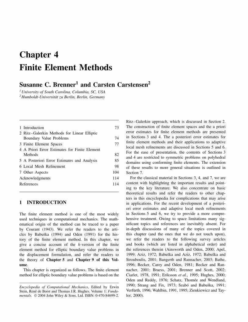
u ∈ H 5/3−ε(D) for any ε > 0, but u ∈ H 5/3(D) (see Triebel(1978) and Grisvard (1985) for a discussion of Besovspaces and fractional order Sobolev spaces). A similar situ-ation occurs when the types of boundary condition changeabruptly, such as the Poisson problem with mixed bound-ary conditions depicted on the circular domain in Figure 1,where the homogeneous Dirichlet boundary condition isassumed on the upper semicircle and the homogeneousNeumann boundary condition is assumed on the lowersemicircle.
Therefore (Dauge, 1988), for the second (respectivelyfourth) order model problems in Section 2.1, the solutionin general only belongs to H 1+α(�) (respectively H 2+α(�))for some α ∈ (0, 1] even if the right-hand side of theequation belongs to C∞(�).
Finite Element Methods 77
u = 0
−∆u = f
u/ n = 0u = 0
−∆u = f
(0,0)
(−1,−1) (1,−1)
(0,1)(−1,1)
(1,0)
Figure 1. Singular points of two-dimensional elliptic boundaryvalue problems.
For two-dimensional problems, the vertices of � and thepoints where the boundary condition changes type are thesingular points (cf. Figure 1). Away from these singularpoints, the Shift Theorem is valid. The behavior of thesolution near the singular points is also well understood.If the right-hand side function and its derivatives vanishto sufficiently high order at the singular points, then theShift Theorem holds for certain weighted Sobolev spaces(Nazarov and Plamenevsky, 1994; Kozlov, Maz’ya andRossman, 1997, 2001). Alternatively, one can represent thesolution near a singular point as a sum of a regular partand a singular part (Grisvard, 1985; Dauge, 1988; Nicaise,1993). For a 2m-th order problem, the regular part of thesolution belongs to the Sobolev space H 2m+k(�) if theright-hand side function belongs to Hk(�), and the singularpart of the solution is a linear combination of specialfunctions with less regularity, analogous to the functionin (28).
The situation in three dimensions is more complicateddue to the presence of edge singularities, vertex singular-ities, and edge-vertex singularities. The theory of three-dimensional singularities remains an active area of research.
3 FINITE ELEMENT SPACES
Finite element methods are Ritz–Galerkin methods wherethe finite-dimensional trial/test function spaces are con-structed by piecing together polynomial functions definedon (small) parts of the domain �. In this section, wedescribe the construction and properties of finite elementspaces. We will concentrate on conforming finite elementshere and leave the discussion of nonconforming finite ele-ments to Section 7.2.
3.1 The concept of a finite element
A d-dimensional finite element (Ciarlet, 1978; Brennerand Scott, 2002) is a triple (K,PK,NK), where K is aclosed bounded subset of R
d with nonempty interior and
a piecewise smooth boundary, PK is a finite-dimensionalvector space of functions defined on K and NK is a basis ofthe dual space P ′K . The function space PK is the space ofthe shape functions and the elements of NK are the nodalvariables (degrees of freedom).
The following are examples of two-dimensional finiteelements.
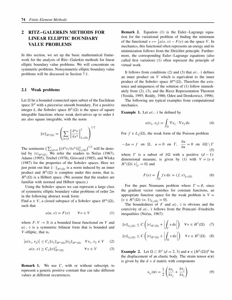
Example 4 (Triangular Lagrange Elements) Let K be atriangle, PK be the space Pn of polynomials in two variablesof degree ≤ n, and let the set NK consist of evaluations ofshape functions at the nodes with barycentric coordinatesλ1 = i/n, λ2 = j/n and λ3 = k/n, where i, j, k are non-negative integers and i + j + k = n. Then (K,PK,NK)
is the two-dimensional Pn Lagrange finite element. Thenodal variables for the P1, P2, and P3 Lagrange elementsare depicted in Figure 2, where • (here and in the fol-lowing examples) represents pointwise evaluation of shapefunctions.
Example 5 (Triangular Hermite Elements) Let K be atriangle. The cubic Hermite element is the triple (K, P3,
NK) where NK consists of evaluations of shape functionsand their gradients at the vertices and evaluation of shapefunctions at the center of K . The nodal variables for thecubic Hermite element are depicted in the first figure inFigure 3, where Ž (here and in the following examples) rep-resents pointwise evaluation of gradients of shape functions.
By removing the nodal variable at the center (cf. thesecond figure in Figure 3) and reducing the space of shapefunctions to{
v ∈ P3: 6v(c)− 23∑
i=1
v(pi)
+3∑
i=1
(∇v)(pi) · (pi − c) = 0}(⊃ P2)
where pi (i = 1, 2, 3) and c are the vertices and center ofK respectively, we obtain the Zienkiewicz element.
The fifth degree Argyris element is the triple (K, P5,NK)
where NK consists of evaluations of the shape functions andtheir derivatives up to order two at the vertices and evalua-tions of the normal derivatives at the midpoints of the edges.The nodal variables for the Argyris element are depictedin the third figure in Figure 3, where © and ↑ (here and
Figure 2. Lagrange elements.

78 Finite Element Methods
Figure 3. Cubic Hermite element, Zienkiewicz element, fifthdegree Argyris element and Bell element.
in the following examples) represent pointwise evaluationof second order derivatives and the normal derivative of theshape functions, respectively.
By removing the nodal variables at the midpoints of theedges (cf. the fourth figure in Figure 3) and reducing thespace of shape functions to {v ∈ P5: (∂v/∂n)
∣∣e∈ P3(e) for
each edge e}, we obtain the Bell element.
Example 6 (Triangular Macro Elements) Let K bea triangle that is subdivided into three subtriangles bythe center of K , PK be the space of piecewise cubicpolynomials with respect to this subdivision that belongto C1(K), and let the set NK consist of evaluations ofthe shape functions and their first-order derivatives at thevertices of K and evaluations of the normal derivatives ofthe shape functions at the midpoints of the edges of K . Then(K,PK,NK) is the Hsieh–Clough–Tocher macro element.The nodal variables for this element are depicted in the firstfigure in Figure 4.
By removing the nodal variables at the midpoints ofthe edges (cf. the second figure in Figure 4) and reducingthe space of shape functions to {v ∈ C1(K): v is piecewisecubic and (∂v/∂n)
∣∣e∈ P1(e) for each edge e}, we obtain
the reduced Hsieh–Clough–Tocher macro element.
Example 7 (Rectangular Tensor Product Elements)Let K be the rectangle [a1, b1]× [a2, b2], PK be thespace spanned by the monomials xi
1xj
2 for 0 ≤ i, j ≤ n,and the set NK consist of evaluations of shape functions
Figure 4. Hsieh–Clough–Tocher element and reduced Hsieh–Clough–Tocher element.
Figure 5. Tensor product elements.
Figure 6. Qn quadrilateral elements.
at the nodes with coordinates(a1 + i(b1 − a1)/n, a2 +
j (b2 − a2)/n)
for 0 ≤ i, j ≤ n. Then (K,PK,NK) is thetwo-dimensional Qn tensor product element. The nodalvariables of the Q1, Q2 and Q3 elements are depicted inFigure 5.
Example 8 (Quadrilateral Qn Elements) Let K bea convex quadrilateral; then there exists a bilinear map(x1, x2) �→ B(x1, x2) = (a1 + b1x1 + c1x2 + d1x1x2, a2 +b2x1 + c2x2 + d2x1x2) from the biunit square S with ver-tices (±1,±1) onto K . The space of shape functions isdefined by v ∈ PK if and only if v ◦B ∈ Qn and NK con-sists of pointwise evaluations of the shape functions at thenodes of K corresponding under the map B to the nodes ofthe Qn tensor product element on S. The nodal variablesof the Q1, Q2 and Q3 quadrilateral elements are depictedin Figure 6.
Example 9 (Other Rectangular Elements) Let K be therectangle [a1, b1]× [c1, d1];
PK ={v ∈ Q2: 4v(c)+
4∑i=1
v(pi)
− 24∑
i=1
v(mi) = 0}(⊃ P2)
where the pi’s are the vertices of K , the mi’s are themidpoints of the edges of K and c is the center of K ;and NK consist of evaluations of the shape functions at thevertices and the midpoints (cf. the first figure in Figure 7).Then (K,PK,NK) is the 8-node serendipity element.
If we take PK to be the space of bicubic polynomialsspanned by xi
1xj
2 for 0 ≤ i, j ≤ 3 and NK to be the set con-sisting of evaluations at the vertices of K of the shape func-tions, their first-order derivatives and their second-order
Figure 7. Serendipity and Bogner–Fox–Schmit elements.
Finite Element Methods 79
mixed derivatives, then we have the Bogner–Fox–Schmitelement. The nodal variables for this element are depictedin the second figure in Figure 7, where the tilted arrowsrepresent pointwise evaluations of the second-order mixedderivatives of the shape functions.
Remark 4. The triangular Pn elements and the quadri-lateral Qn elements, which are suitable for second orderelliptic boundary value problems, can be generalized toany dimension in a straightforward manner. The Argyriselement, the Bell element, the macro elements, and theBogner–Fox–Schmit element are suitable for fourth-orderproblems in two space dimensions.
3.2 Triangulations and finite element spaces
We restrict � ⊂ Rd (d = 1, 2, 3) to be a polyhedral domain
in this and the following sections. The case of curveddomains will be discussed in Section 7.4.
A partition of � is a collection P of polyhedral subdo-mains of � such that
� =⋃D∈P
D and D ∩D′ = ∅ if D, D′ ∈ P, D = D′
where we use � and D to represent the closures of �
and D.A triangulation of � is a partition where the intersection
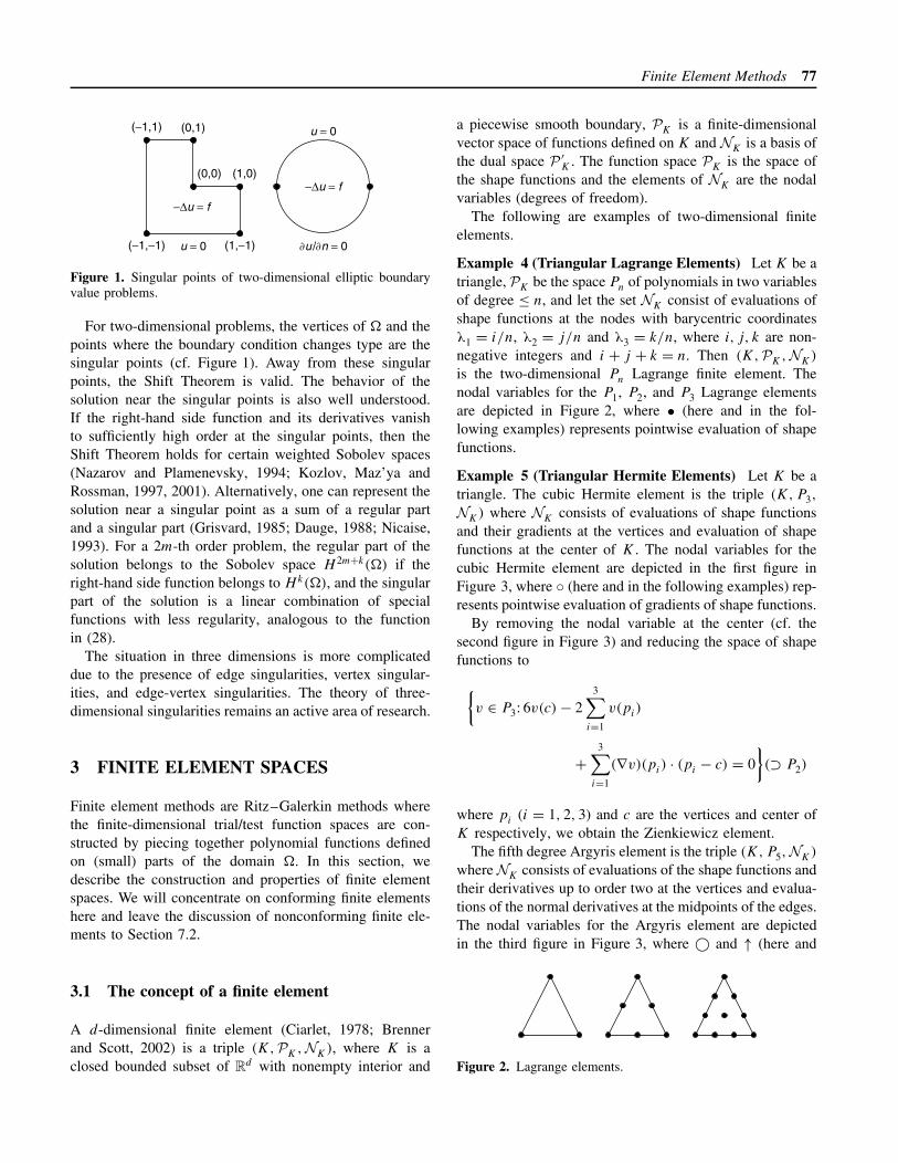
of the closures of two distinct subdomains is either empty,a common vertex, a common edge or a common face.For d = 1, every partition is a triangulation. But the twoconcepts are different when d ≥ 2. A partition that is not atriangulation is depicted in the first figure in Figure 8, wherethe other three figures represent triangulations. Below wewill concentrate on triangulations consisting of triangles orconvex quadrilaterals in two dimensions and tetrahedronsor convex hexahedrons in three dimensions.
The shape regularity of a triangle (or tetrahedron) D canbe measured by the parameter
γ(D) = diam D
diameter of the largest ball in D(29)
which will be referred to as the aspect ratio of the trian-gle (tetrahedron). We say that a family of triangulations of
Figure 8. Partitions and triangulations.
triangles (or tetrahedrons) {Ti : i ∈ I } is regular (or nonde-generate) if the aspect ratios of all the triangles (tetrahe-drons) in the triangulations are bounded, that is, there existsa positive constant C such that
γ(D) ≤ C for all D ∈ Ti and i ∈ I
The shape regularity of a convex quadrilateral (or hexa-hedron) D can be measured by the parameter γ(D) definedin (29) and the parameter
σ(D) = max{ |e1||e2|
: e1 and e2 are any two edges of D
}(30)
We will refer to the number max(γ(D), σ(D)) as the aspectratio of the convex quadrilateral (hexahedron). We saythat a family of triangulations of convex quadrilaterals (orhexahedrons) {Ti : i ∈ I } is regular if the aspect ratios of allthe quadrilaterals in the triangulations are bounded, that is,there exists a positive constant C such that
γ(D), σ(D) ≤ C for all D ∈ Ti and i ∈ I
A family of triangulations is quasi-uniform if it is regularand there exists a positive constant C such that
hi ≤ C diam D ∀D ∈ Ti , i ∈ I (31)
where hi is the maximum of the diameters of the subdo-mains in Ti .
Remark 5. For a triangle or a tetrahedron D, a lowerbound for the angles of D can lead to an upper bound forγ(D) (and vice versa). Therefore, the regularity of a familyof simplicial triangulations (i.e. triangulations consisting oftriangles or tetrahedrons) is equivalent to the followingminimum angle condition: There exists θ∗ > 0 such thatthe angles of the simplexes in all the triangulations Ti arebounded below by θ∗.
Remark 6. A family of triangulations obtained by suc-cessive uniform subdivisions of an initial triangulation isquasi-uniform. A family of triangulations generated by alocal refinement strategy is usually regular but not quasi-uniform.
Let T be a triangulation of �, and a finite element(D,P
D,N
D) be associated with each subdomain D ∈ T.
We define the corresponding finite element space to be
FET = {v ∈ L2(�): vD= v
∣∣D∈ P
D∀D ∈ T, and
vD, v
D′ share the same nodal values on D ∩D
′}(32)

80 Finite Element Methods
We say that FET is a Cr finite element space if FET ⊂Cr(�). For example, the finite element spaces constructedfrom the Lagrange finite elements (Example 4), the tensorproduct elements (Example 7), the cubic Hermite element(Example 4), the Zienkiewicz element (Example 4) andthe serendipity element (Example 9) are C0 finite elementspaces, and those constructed from the quintic Argyris ele-ment (Example 5), the Bell element (Example 5), the macroelements (Example 6) and the Bogner–Fox–Schmit ele-ment (Example 9) are C1 finite element spaces.
Note that a Cr finite element space is automaticallya subspace of the Sobolev space Hr+1(�) and thereforeappropriate for elliptic boundary value problems of order2(r + 1).
3.3 Element nodal interpolation operators andinterpolation error estimates
Let (K,PK,NK) be a finite element. Denote the nodalvariables in NK by N1, . . . , Nn (n = dimPK ) and the dualbasis of PK by φ1, . . . , φn, that is,
Ni(φj ) = δij ={
1 if i = j
0 if i = j
Assume that ζ �→ Ni(ζ) is well-defined for ζ ∈ Hs(K)
(where s is a sufficiently large positive number), thenwe can define the element nodal interpolation operator�K : Hs(K)→ PK by
�Kζ =n∑
j=1
Nj(ζ)φj (33)
Note that (33) implies
�Kv = v ∀ v ∈ PK (34)
For example, by the Sobolev embedding theorem(Adams, 1995; Necas, 1967; Wloka, 1987; Gilbargand Trudinger, 1983), the nodal interpolation operatorsassociated with the Lagrange finite elements (Example 4),the tensor product finite elements (Example 7), andthe serendipity element (Example 9) are well-defined onHs(K) for s > 1 if K ⊂ R
2 and for s > 3/2 if K ⊂ R3. On
the other hand the nodal interpolation operators associatedwith the Zienkiewicz element (Example 5) and the macroelements (Example 6) are well-defined on Hs(K) for s > 2,while the interpolation operators for the quintic Argyriselement (Example 5), the Bell element (Example 5) orthe Bogner–Fox–Schmit (Example 9) are well-defined onHs(K) for s > 3.
The error of the element nodal interpolation operator for atriangular (tetrahedral) or convex quadrilateral (hexagonal)
element (K,PK,NK) can be controlled in terms of theshape regularity of K . Let K be the image of K underthe scaling map
x �→ H(x) = (diam K)−1x (35)
Then K is a domain of unit diameter and we can define afinite element (K,P
K,N
K) as follows: (i) v ∈ P
Kif and
only if v ◦H ∈ PK , and (ii) N ∈ NK
if and only if thelinear functional v �→ N(v ◦H−1) on PK belongs to NK .It follows that the dual basis φ1, . . . , φn of P
Kis related
to the dual basis φ1, . . . ,φn of PK through the relationφi ◦H = φi , and (33) implies that
(�Kζ) ◦H−1 = �K(ζ ◦H−1) (36)
for all sufficiently smooth functions ζ defined on K . More-over, for the functions ζ and ζ related by ζ(x) = ζ(H(x)),we have
|ζ|2Hs(K)
= (diam K)2s−d |ζ|2Hs(K) (37)
where d is the spatial dimension.Assuming that P
K⊇ Pm (equivalently PK ⊇ Pm), we
have, by (34),
‖ζ−�Kζ‖
Hm(K)= ‖(ζ− p)−�
K(ζ− p)‖
Hm(K)
≤ 2‖�K‖m,s ‖ζ− p‖
Hs(K)∀p ∈ Pm
where ‖�K‖m,s is the norm of the operator �
K: Hs(K) →
Hm(K), and hence
‖ζ−�Kζ‖
Hm(K)≤ 2‖�
K‖m,s inf
p∈Pm
‖ζ− p‖Hs(K)
(38)
Since K is convex, the following estimate (Verfurth,1999) holds provided m is the largest integer strictly lessthan s:
infp∈Pm
‖ζ− p‖Hs(K)
≤ Cs,d |ζ|Hs(K)∀ ζ ∈ Hs(K) (39)
where the positive constant Cs,d depends only on s and d .Combining (38) and (39) we find
‖ζ−�Kζ‖
Hm(K)≤ 2Cs,d‖�K
‖m,s |ζ|Hs(K)∀ ζ ∈ Hs(K)
(40)
We have therefore reduced the error estimate for theelement nodal interpolation operator to an estimate of‖�
K‖m,s . Since diam K = 1, the norm ‖�
K‖m,s is a con-
stant depending only on the shape of K (equivalently ofK), if we considered s and m to be fixed for a given typeof element.
For triangular elements, we can use the concept of affine-interpolation-equivalent elements to obtain a more concrete

Finite Element Methods 81
description of the dependence of ‖�K‖m,s on the shape
of K . A d-dimensional nondegenerate affine map is amap of the form x �→ Ax + b where A is a nonsingulard × d matrix and b ∈ R
d . We say that two finite elements(K1,PK1
,NK1) and (K2,PK2
,NK2) are affine-equivalent if
(i) there exists a nondegenerate affine map � that maps K1onto K2, (ii) v ∈ PK2
if and only if v ◦� ∈ PK1and (iii)
(�K2ζ) ◦� = �K1
(ζ ◦�) (41)
for all sufficiently smooth functions ζ defined on K2. Forexample, any triangular elements in one of the families(except the Bell element and the reduced Hsieh–Clough–Tocher element) described in Section 3.1 are affine-interpolation-equivalent to the corresponding element onthe standard simplex S with vertices (0, 0), (1, 0) and (0, 1).
Assuming (K,PK,N
K) (or equivalently (K,PK,NK))
is affine-interpolation-equivalent to the element (S,PS,NS)
on the standard simplex, it follows from (41) and the chainrule that
‖�K‖m,s ≤ C‖�S‖m,s (42)
where the positive constant depends only on the Jacobianmatrix of the affine map �: S → K and thus depends onlyon an upper bound of the parameter γ(K) (cf. (29)) whichis identical with γ(K).
Combining (36), (37), (40) and (42), we find
m∑k=0
(diam K)k|ζ−�Kζ|Hm(K)
≤ C(diam K)s |ζ|Hs(K)
∀ ζ ∈ Hs(K) (43)
where the positive constant C depends only on s andan upper bound of the parameter γ(K) (the aspect ratioof K), provided that (i) the element nodal interpolationoperator is well-defined on Hs(K), (ii) the triangular ele-ment (K,PK,NK) is affine-interpolation-equivalent to areference element (S,PS,NS) on the standard simplex,(iii) P ⊇ Pm, and (iv) m is the largest integer < s.
For convex quadrilateral elements, we can similarlyobtain a concrete description of the dependence of ‖�
K‖m,s
on the shape of K by assuming that there is a referenceelement (S,PS,NS) defined on the biunit square S withvertices (±1,±1) and a bilinear homeomorphism � from S
onto K with the following properties: v ∈ PK
if and only ifv ◦� ∈ PS and (�
Kζ) ◦ � = �S(ζ ◦ �) for all sufficiently
smooth functions ζ defined on K . Note that because of (36)
this is equivalent to the existence of a bilinear homeomor-phism from S onto K such that
v ∈ PK ⇐�⇒ v ◦� ∈ PS and (�Kζ) ◦� = �S(ζ ◦�)
(44)
for all sufficiently smooth functions ζ defined on K . Theestimate (42) holds again by the chain rule, where thepositive constant C depends only on the Jacobian matrixof � and thus depends only on upper bounds for theparameters γ(K) and σ(K) (cf. (30)), which are identicalwith γ(K) and σ(K). We conclude that the estimate (43)also holds for convex quadrilateral elements where thepositive constant C depends on upper bounds of γ(K) andσ(K) (equivalently an upper bound of the aspect ratio ofK) provided condition (ii) is replaced by (44). For example,the estimate (43) is valid for the quadrilateral Qn elementin Example 8.
Remark 7. The general estimate (40) can be refinedto yield anisotropic error estimates for certain referenceelements. For example, in two dimensions, the followingestimates (Apel and Dobrowolski, 1992; Apel, 1999) holdfor the Pn Lagrange elements on the reference simplexS and the Qn tensor product elements on the referencesquare S:∥∥∥∥∥ ∂
∂xj
(ζ−�Sζ)
∥∥∥∥∥L2(S)
≤ C
(∥∥∥∥∥ ∂2ζ
∂x1∂xj
∥∥∥∥∥L2(S)
+∥∥∥∥∥ ∂2ζ
∂x2∂xj
∥∥∥∥∥L2(S)
)(45)
for j = 1, 2 and for all ζ ∈ H 2(S). We refer the readers toChapter 3, this Volume, for more details.
Remark 8. The analysis of the quadrilateral serendipityelements is more subtle. A detailed discussion can be foundin Arnold, Boffi and Falk (2002).
Remark 9. The estimate (43) can be generalized naturallyto 3-D tetrahedral Pn elements and hexahedral Qn elements.
Remark 10. Let n be a nonnegative integer and n < s ≤n+ 1. The estimate
infp∈Pn(�)
‖ζ− p‖Hs(�) ≤ C�,s |ζ|Hs(�) ∀ ζ ∈ Hs(�)
(46)
for general � follows from generalized Poincare–Friedrichsinequalities (Necas, 1967). In the case where � is convex,the constant C�,s depends only on s and the dimensionof �, but not on the shape of �, as indicated by theestimate (39). For nonconvex domains, the constant C�,s

82 Finite Element Methods
does depend on the shape of � (Dupont and Scott, 1980,Verfurth, 1999).
Let F be a bounded linear functional on Hs(�) withnorm ‖F‖ such that F(p) = 0 for all p ∈ Pn(�). It followsfrom (46) that
|F(ζ)| ≤ infp∈Pn(�)
|F(ζ− p)| ≤ ‖F‖ infp∈Pn(�)
‖ζ− p‖Hs(�)
≤ (C�,s‖F‖)|ζ|Hs(�) (47)
for all ζ ∈ Hs(�). The estimate (47), known as the Bram-ble–Hilbert lemma (Bramble and Hilbert, 1970), is usefulfor deriving various error estimates.
3.4 Some discrete estimates
The finite element spaces in Section 3.2 are designed tobe subspaces of Sobolev spaces so that they can serveas the trial/test spaces for Ritz–Galerkin methods. On theother hand, since finite element spaces are constructed bypiecing together finite-dimensional function spaces, thereare discrete estimates valid on the finite element spaces butnot the Sobolev spaces.
Let (K,PK,NK) be a finite element such that PK ⊂Hk(K) for a nonnegative integer k. Since any seminormon a finite-dimensional space is continuous with respect toa norm, we have, by scaling, the following inverse estimate:
|v|Hk(K) ≤ C(diam K)�−k‖v‖H�(K) ∀ v ∈ PK, 0 ≤ � ≤ k
(48)
where the positive constant C depends on the domain K
(the image of K under the scaling map H defined by (35))and the space PK .
For finite elements whose shape functions can be pulledback to a fixed finite-dimensional function space on areference element, the constant C depends only on the shaperegularity of the element domain K and global versionsof (48) can be easily derived. For example, for a quasi-uniform family {Ti : i ∈ I } of simplicial or quadrilateraltriangulations of a polygonal domain �, we have
|v|H 1(�) ≤ Ch−1i ‖v‖L2(�) ∀ v ∈ Vi and i ∈ I (49)
where Vi ⊂ H 1(�) is either the Pn triangular finite elementspace or the Qn quadrilateral finite element space associatedwith Ti . Note that Vi ⊂ Hs(�) for any s < 3/2 and a bitmore work shows that the following inverse estimate (BenBelgacem and Brenner, 2001) also holds:
|v|Hs(�) ≤ Csh1−si ‖v‖H 1(�) ∀ v ∈ Vi, i ∈ I and
1 ≤ s < 3/2 (50)
where the positive constant Cs can be uniformly boundedfor s in a compact subset of [1, 3/2).
It is well-known that in two dimensions the Sobolevspace H 1(�) is not a subspace of C(�). However, thePn triangular finite element space and the Qn quadrilateralfinite element space do belong to C(�) and it is possibleto bound the L∞ norm of the finite element function byits H 1 norm. Indeed, it follows from Fourier transformand extension theorems (Adams, 1995, Wloka, 1987) that,for ε > 0,
‖v‖L∞(�) ≤ Cε−1/2‖v‖H 1+ε(�) ∀ v ∈ H 1+ε(�) (51)
By taking ε = (1+ | ln hi |)−1 in (51) and applying (50), wearrive at the following discrete Sobolev inequality:
‖v‖L∞(�) ≤ C(1+ | ln hi |)1/2‖v‖H 1(�) ∀ v ∈ Vi and
i ∈ I (52)
where the positive constant C is independent of i ∈ I .The discrete Sobolev inequality and the Poincare–Fried-
richs inequality (8) imply immediately the following dis-crete Poincare inequality:
‖v‖L∞(�) ≤ ‖v − v‖L∞(�) + ‖v‖L∞(�) ≤ 2‖v − v‖L∞(�)
≤ C(1+ | ln hi |)1/2‖v − v‖H 1(�)
≤ C(1+ | ln hi |)1/2|v|H 1(�) (53)
for all v ∈ Vi that vanishes at a given point in � and withmean v = ∫
�v dx/|�|.
Remark 11. The discrete Sobolev inequality can also beestablished directly using calculus and inverse estimates(Bramble, Pasciak and Schatz, 1986; Brenner and Scott,2002), and both (52) and (53) are sharp (Brenner and Sung,2000).
4 A PRIORI ERROR ESTIMATES FORFINITE ELEMENT METHODS
Let T be a triangulation of � and a finite element(D,P
D,N
D) be associated with each subdomain D ∈ T so
that the resulting finite element space FET (cf. (32)) is asubspace of Cm−1(�) ⊂ Hm(�). By imposing appropriateboundary conditions, we can obtain a subspace VT of FETsuch that VT ⊂ V , the subspace of Hm(�), where the weakproblem (1) is formulated. The corresponding finite elementmethod for (1) is:Find uT ∈ VT such that
a(uT, v) = F(v) ∀ v ∈ VT (54)
Finite Element Methods 83
In this section, we consider a priori estimates for thediscretization error u− uT. We will discuss the second-order and fourth-order cases separately. We use the letter C
to denote a generic positive constant that can take differentvalues at different appearances.
Let us also point out that the asymptotic error analysiscarried out in this section is not sufficient for parameter-dependent problems (e.g. thin structures and nearly incom-pressible elasticity) that can experience locking (Babuskaand Suri, 1992). We refer the readers to other chaptersin this encyclopedia that are devoted to such problemsfor the discussion of the techniques that can overcomelocking.
4.1 Second-order problems
We will devote most of our discussion to the case where� ⊂ R
2 and only comment briefly on the 3-D case. For pre-ciseness, we also assume the right-hand side of the ellipticboundary value problem to be square integrable. We firstconsider the case where V ⊂ H 1(�) is defined by homo-geneous Dirichlet boundary conditions (cf. Section 2.1) on� ⊂ ∂�. Such problems can be discretized by triangular Pn
elements (Example 4) or quadrilateral Qn elements (Exam-ple 8).
Let T be a triangulation of � by triangles (convex quadri-laterals) and each triangle (quadrilateral) in T be equippedwith the Pn (n ≥ 1) Lagrange element (Qn quadrilateralelement). The resulting finite element space FET is a sub-space of C0(�) ⊂ H 1(�). We assume that � is the unionof the edges of the triangles (quadrilaterals) in T and takeVT = V ∩ FET , the subspace defined by the homogeneousDirichlet boundary condition on �.
We know from the discussion in Section 2.3 that u ∈H 1+α(D)(D) for each D ∈ T, where the number α(D) ∈(0, 1] and α(D) = 1 for D away from the singular points.Hence, the element nodal interpolation operator �
Dis well-
defined on u for all D ∈ T. We can therefore piece togethera global nodal interpolant � N
T u ∈ VT by the formula(�N
T u)∣∣
D= �
D
(u∣∣D
)(55)
From the discussion in Section 3.3, we know that (43) isvalid for both the triangular Pn element and the quadrilat-eral Qn element. We deduce from (43) and (55) that
‖u−�NT u‖2
H 1(�)≤ C
∑D∈T
(diam D)2α(D)|u|2H 1+α(D)(D)
(56)
where C depends only on the maximum of the aspect ratiosof the element domains in T. Combining (22) and (56) we
have the a priori discretization error estimate
‖u− uT ‖H 1(�) ≤ C(∑
D∈T(diam D)2α(D)|u|2
H 1+α(D)(D)
)1/2
(57)
where C depends only on the constants in (2) and (3) andthe maximum of the aspect ratios of the element domainsin T.
Hence, if {Ti : i ∈ I } is a regular family of triangulations,and the solution u of (1) belongs to the Sobolev spaceH 1+α(�) for some α ∈ (0, 1], then we can deduce from(57) that
‖u− uTi‖H 1(�) ≤ Chα
i |u|H 1+α(�) (58)
where hi = maxD∈Tidiam D is the mesh size of Ti and C is
independent of i ∈ I . Note that the solution w of (23) withu replaced by uT also belongs to H 1+α(�) and satisfies theelliptic regularity estimate
‖w‖H 1+α(�) ≤ C‖u− uT ‖L2(�)
Therefore, we have
infv∈VT
‖w − v‖H 1(�) ≤ ‖w −� NT w‖H 1(�) ≤ Chα
i |w|H 1+α(�)
≤ Chαi ‖u− uT ‖L2(�) (59)
The abstract estimate (24) with u replaced by uT and (59)yield the following L2 estimate:
‖u− uTi‖L2(�) ≤ Ch2α
i |u|H 1+α(�) (60)
where C is also independent of i ∈ I .
Remark 12. In the case where α = 1 (for example, when� = ∂� in Example 1 and � is convex), the estimate (58) isoptimal and it is appropriate to use a quasi-uniform familyof triangulations. In the case where α(D) < 1 for D nextto singular points, the estimate (57) allows the possibilityof improvement by graded meshes (cf. Section 6).
Remark 13. In the derivations of (58) and (60) abovefor the triangular Pn elements, we have used the minimumangle condition (cf. Remark 5). In view of the anisotropicestimates (45), these estimates also hold for triangular Pn
elements under the maximum angle condition (Babuska andAziz, 1976; Jamet, 1976; Zenisek, 1995; Apel, 1999): thereexists θ∗ < π such that all the angles in the family oftriangulations are ≤ θ∗. The estimates (58) and (60) arealso valid for Qn elements on parallelograms satisfying themaximum angle condition. They can also be established forcertain thin quadrilateral elements (Apel, 1999).
84 Finite Element Methods
The 2-D results above also hold for 3-D tetrahedral Pn
elements and 3-D hexagonal Qn elements if the solutionu of (1) belongs to H 1+α(�) where 1/2 < α ≤ 1, sincethe nodal interpolation operator are then well-defined bythe Sobolev embedding theorem. This is the case, forexample, if � = ∂� in Example 1. However, new inter-polation operators that require less regularity are needed if0 < α ≤ 3/2. Below, we construct an interpolation opera-tor �A
T : H 1(�) → VT using the local averaging techniqueof Scott and Zhang (1990).
For simplicity, we take VT to be a tetrahedral P1 finiteelement space. Therefore, we only need to specify thevalue of �A
T ζ at the vertices of T for a given functionζ ∈ H 1(�). Let p be a vertex. We choose a face (oredge in 2-D) F of a subdomain in T such that p ∈ F.The choice of F is of course not unique. But we alwayschoose F ⊂ ∂� if p ∈ ∂� so that the resulting interpolantwill satisfy the appropriate Dirichlet boundary condition.Let {ψj }dj=1 ⊂ P1(F) be biorthogonal to the nodal basis{φj }dj=1 ⊂ P1(F) with respect to the L2(F) inner product.In other words φj equals 1 at the j th vertex of F andvanishes at the other vertices, and∫
Fψiφj ds = δij (61)
Suppose p corresponds to the j th vertex of F. We thendefine
(�AT ζ)(p) =
∫F
ψj ζ ds (62)
where the integral is well-defined because of the tracetheorem.
It is clear in view of (61) and (62) that �AT v = v for
all v ∈ FET and �AT ζ = 0 on � if ζ = 0 on �. Note also
that �AT is not a local operator, i.e., (�A
T ζ)∣∣D
is in generaldetermined by ζ
∣∣S(D)
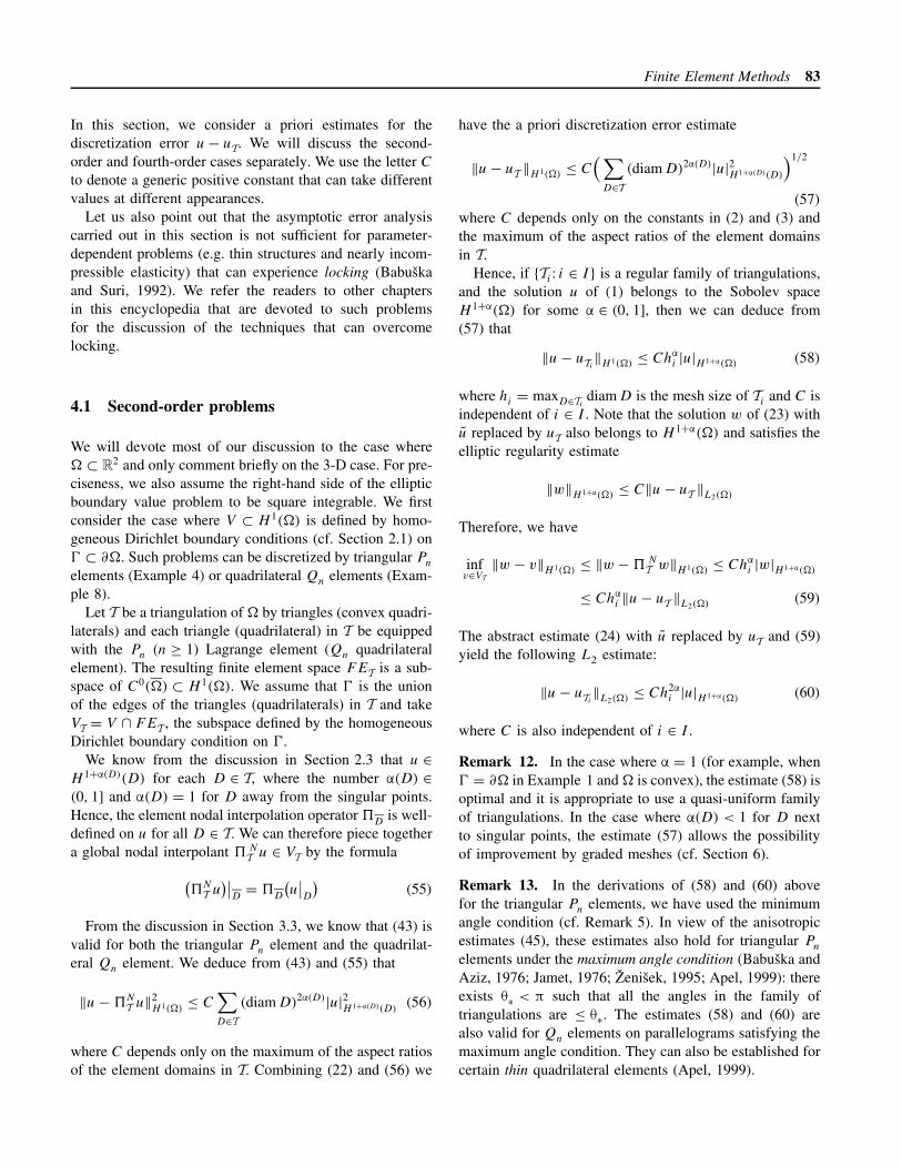
, where S(D) is the polyhedral domainformed by the subdomains in T sharing (at least) a vertexwith D (cf. Figure 9 for a 2-D example). It follows thatthe interpolation error estimate for �T takes the followingform:
‖ζ−�AT ζ‖2
L2(D) + (diam D)2|ζ−�AT ζ|2
H 1(D)
≤ C(diam D)2(1+α(S(D)))|ζ|2
H 1+α(S(D))(S(D))
(63)
where C depends on the shape regularity of T, providedthat ζ ∈ H 1+α(S(D))(S(D)) for some α(S(D)) ∈ (0, 1]. Theestimates (58) and (60) for tetrahedral P1 elements canbe derived for general α ∈ (0, 1] and regular triangulationsusing the estimate (63).
D
Figure 9. A two-dimensional example of S(D).
Remark 14. The interpolation operator �AT can be defined
for general finite elements (Scott and Zhang, 1990; Giraultand Scott, 2002) and anisotropic estimates can be obtainedfor �A
T for certain triangulations (Apel, 1999). Therealso exist interpolation operators for less regular functions(Clement, 1975; Bernardi and Girault, 1998).
Next, we consider the case where V is a closed subspaceof H 1(�) with finite codimension n < ∞, as in the caseof the Poisson problem with pure homogeneous Neumannboundary condition (where n = 1) or the elasticity problemwith pure homogeneous traction boundary condition (wheren = 1 when d = 1, and n = 3(d − 1) when d = 2 or 3).The key assumption here is that there exists a boundedlinear projection Q from H 1(�) onto an n dimensionalsubspace of FET such that ζ ∈ H 1(�) belongs to V if andonly if Qζ = 0. We can then define an interpolation operator�T from appropriate Sobolev spaces onto VT by
�T = (I −Q)�T
where �T is either the nodal interpolation operator �NT
or the Scott–Zhang averaging interpolation operator �AT
introduced earlier. Observe that, since the weak solution u
belongs to V ,
u− �Tu = u−Qu− (I −Q)�Tu = (I −Q)(u−�Tu)
and the interpolation error of �T can be estimated in termsof the norm of Q: H 1(�) → H 1(�) and the interpolationerror of �T . Therefore, the a priori discretization error esti-mates for Dirichlet or Dirichlet/Neumann boundary valueproblems also hold for this second type of (pure Neumann)boundary value problems.
For the Poisson problem with homogeneous Neumannboundary condition, we can take
Qζ = 1
|�|∫
�
ζ dx
the mean of ζ over �. For the elasticity problem with purehomogeneous traction boundary condition, the operator Q
from [H 1(�)]d onto the space of infinitesimal rigid motions
Finite Element Methods 85
is defined by∫�
Qζ dx =∫
�
ζ dx and∫�
∇ ×Qζ dx =∫
�
∇ × ζ dx ∀ ζ ∈ [H 1(�)]d
In both cases, the norm of Q is bounded by a constant C�.
Remark 15. In the case where f ∈ Hk(�) for k > 0, thesolution u belongs to H 2+k(�) away from the geometricor boundary data singularities and, in particular, awayfrom ∂�. Therefore, it is advantageous to use higher-order elements in certain parts of �, or even globally(with curved elements near ∂�) if singularities are notpresent. In the case where f ∈ L2(�), the error estimate(57) indicates that the order of the discretization error forthe triangular Pn element or the quadrilateral Qn elementis independent of n ≥ 1. However, the convergence of thefinite element solutions to a particular solution as h ↓ 0can be improved by using higher-order elements becauseof the existence of nonuniform error estimates (Babuskaand Kellogg, 1975).
4.2 Fourth-order problems
We restrict the discussion of fourth-order problems to thetwo-dimensional plate bending problem of Example 3.
Let T be a triangulation of � by triangles and eachtriangle in T be equipped with the Hsieh–Clough–Tochermacro element (cf. Example 6). The finite element spaceFET defined by (32) is a subspace of C1(�) ⊂ H 2(�). Wetake VT to be V ∩ FET , where V = H 2
0 (�) for the clampedplate and V = H 1
0 (�) ∩H 2(�) for the simply supportedplate.
The solution u of the plate-bending problem belongsto H 2+α(D)(D) for each D ∈ T, where α(D) ∈ (0, 2] andα(D) = 2 for D away from the corners of �. The ele-mental nodal interpolation operator �
Dis well-defined
on u for all D ∈ T. We can therefore define a globalnodal interpolation operator �N
T by the formula (55).Since the Hsieh–Clough–Tocher macro element is affine-interpolation-equivalent to the reference element on thestandard simplex, we deduce from (55) and (43) that
‖u−�NT u‖2
H 2(�)≤ C
∑D∈T
(diam D)2α(D)|u|2H 2+α(D)(D)
(64)
where C depends only on the maximum of the aspect ratiosof the triangles in T (or equivalently the minimum angle of
T ). From (22) and (64), we have
‖u− uT ‖H 2(�) ≤ C
(∑D∈T
(diam D)2α(D)|u|2H 2+α(D)(D)
)1/2
(65)
where C depends only on the constants in (2) and (3) andthe minimum angle of T.
Hence, if {Ti : i ∈ I } is a regular family of triangulations,and the solution u of the plate bending problem belongsto the Sobolev space H 2+α(�) for some α ∈ (0, 2], we candeduce from (65) that
‖u− uTi‖H 2(�) ≤ Chα
i |u|H 2+α(�) (66)
where hi = maxD∈Tidiam D is the mesh size of Ti and C
is independent of i ∈ I . Since the solution w of (23) alsobelongs to H 2+α(�), the abstract estimate (24) combinedwith an error estimate for w in the H 2-norm analogous to(66) yields the following L2 estimate:
‖u− uTi‖L2(�) ≤ Ch2α
i |u|H 2+α(�) (67)
where C is also independent of i ∈ I .
Remark 16. The analysis of general triangular and quad-rilateral C1 macro elements can be found in Douglas et al.(1979).
The plate-bending problem can also be discretized bythe Argyris element (cf. Example 5). If α(D) > 1 for allD ∈ D, then the nodal interpolation operator �N
T is well-defined for the Argyris finite element space. If α(D) ≤ 1for some D ∈ T, then the nodal interpolation operator �N
Tmust be replaced by an interpolation operator constructedby the technique of local averaging. In either case, theestimates (65)–(67) remain valid for the Argyris finiteelement solution.
5 A POSTERIORI ERROR ESTIMATESAND ANALYSIS
In this section, we review explicit and implicit estimators aswell as averaging and multilevel estimators for a posteriorifinite element error control.
Throughout this section, we adopt the notation of Sec-tions 2.1 and 2.2 and recall that u denotes the (unknown)exact solution of (1) while u ∈ V denotes the discrete andgiven solution of (19). It is the aim of Section 5.1–5.6to estimate the error e := u− u ∈ V in the energy norm‖ · ‖a = (a(·, ·))1/2 in terms of computable quantities whileSection 5.7 concerns other error norms or goal functionals.
86 Finite Element Methods
Throughout this section, we assume 0 < ‖e‖a to excludethe exceptional situation u = u.
5.1 Aims and concepts in a posteriori finiteelement error control
The following five sections introduce the notation, theconcepts of efficiency and reliability, the definitions ofresidual and error, a posteriori error control and adaptivealgorithms, and comment on some relevant literature.
5.1.1 Error estimators, efficiency, reliability,asymptotic exactness
Regarded as an approximation to the (unknown) error norm‖e‖a , a (computable) quantity η is called a posteriori errorestimator, or estimator for brevity, if it is a function of theknown domain � and its boundary �, the quantities of theright-hand side F , cf. (6) and (13), as well as of the (given)discrete solution u, or the underlying triangulation.
An estimator η is called reliable if
‖e‖a ≤ Crel η+ h.o.t.rel (68)
An estimator η is called efficient if
η ≤ Ceff ‖e‖a + h.o.t.eff (69)
An estimator is called asymptotically exact if it is reliableand efficient in the sense of (68)–(69) with Crel = C−1
eff .Here, Crel and Ceff are multiplicative constants that do
not depend on the mesh size of an underlying finite elementmesh T for the computation of u and h.o.t. denotes higher-order terms. The latter are generically much smaller thanη or ‖e‖a , but usually, this depends on the (unknown)smoothness of the exact solution or the (known) smoothnessof the given data. The readers are warned that, in general,h.o.t. may not be neglected; in case of high oscillations theymay even dominate (68) or (69).
5.1.2 Error and residual
Abstract examples for estimators are (26) and (27), whichinvolve dual norms of the residual (25). Notice carefullythat R := F − a(u, ·) is a bounded linear functional in V ,written R ∈ V ∗, and hence the dual norm
‖R‖V ∗ := supv∈V \{0}
R(v)
‖v‖a
= supv∈V \{0}
a(e, v)
‖v‖a
= ‖e‖a < ∞(70)
The second equality immediately follows from (25). ACauchy inequality in (70) with respect to the scalar product
a results in ‖R‖V ∗ ≤ ‖e‖a while v = e in (70) yields finallythe equality ‖R‖V ∗ = ‖e‖a .
That is, the error (estimation) in the energy norm is equiv-alent to the (computation of the) dual norm of the givenresidual. Furthermore, it is even of comparable computa-tional effort to compute an optimal v = e in (70) or tocompute e. The proof of (70) yields even a stability esti-mate: The relative error of R(v) as an approximation to‖e‖a equals(‖e‖a − R(v)
)‖e‖a
= 1
2
∥∥∥∥v − e
‖e‖a
∥∥∥∥2
a
for all v ∈ V with ‖v‖a = 1 (71)
In fact, given any v ∈ V with ‖v‖a = 1, the identity (71)follows from
1− a
(e
‖e‖a
, v
)= 1
2a
(e
‖e‖a
,e
‖e‖a
)− a
(e
‖e‖a
, v
)
+ 1
2a(v, v) = 1
2
∥∥∥∥v − e
‖e‖a
∥∥∥∥2
a
The error estimate (71) implies that the maximizing v in(70) (i.e. v ∈ V with maximal R(v) subject to ‖v‖a ≤1) is unique and equals e/‖e‖a . As a consequence, thecomputation of the maximizing v in (70) is equivalent toand indeed equally expensive as the computation of theunknown e/‖e‖a and so (since u is known) of the exactsolution u. Therefore, a posteriori error analysis aims tocompute lower and upper bounds of ‖R‖V ∗ rather than itsexact value.
5.1.3 Error estimators and error control
For an idealized termination procedure, one is given atolerance Tol > 0 and interested in a stopping criterion (ofsuccessively adapted mesh refinements)
‖e‖a ≤ Tol
Since the error ‖e‖a is unknown, it is replaced by its upperbound (68) and then leads to
Crelη+ h.o.t.rel ≤ Tol (72)
For a verification of (72), in practice, one requires not onlyη but also Crel and h.o.t.rel. The later quantity cannot bedropped; it is not sufficient to know that h.o.t.rel is (possibly)negligible for sufficient small mesh-sizes.
Section 5.6 presents numerical examples and further dis-cussions of this aspect.

Finite Element Methods 87
5.1.4 Adaptive mesh-refining algorithms
Error estimators are used in adaptive mesh-refining algo-rithms to motivate a refinement rule, which determineswhether an element or edge and so on shall be refined orcoarsened. This will be discussed in Section 6below.
At this stage two remarks are in order. First, one shouldbe precise in the language and distinguish between errorestimators, which are usually global and fully involveconstants and higher-order terms and (local) refinementindicators used in refinement rules. Second, constants andhigher-order terms might be seen as less important and areoften omitted in the usage as refinement indicators for thestep MARKING in Section 6.2.
5.1.5 Literature
Amongst the most influential pioneering publications ona posteriori error control are Babuska and Rheinboldt(1978), Ladeveze and Leguillon (1983), Bank and Weiser(1985), Babuska and Miller (1987), Eriksson and Johnson(1991), followed by many others. The readers may find itrewarding to study the survey articles of Eriksson et al.(1995), Becker and Rannacher (2001) and the books ofVerfurth (1996), Ainsworth and Oden (2000), Babuska andStrouboulis (2001), Bangerth and Rannacher (2003) for afirst insight and further references.
5.2 Explicit residual-based error estimators
The most frequently considered and possibly easiest class oferror estimators consists of local norms of explicitly givenvolume and jump residuals multiplied by mesh-dependingweights.
To derive them for a general class of abstract problemsfrom Section 2.1, let u ∈ V be an exact solution of theproblem (1) and let u ∈ V be its Galerkin approximationfrom (19) with residual R(v) from (25). Moreover, as inExample 1 or 2, it is supposed throughout this chapter thatthe strong form of the equilibration associated with theweak form (19) is of the form
−divp = f for some flux or stress p ∈ L2(�;Rm×n)
The discrete analog p is piecewise smooth but, in general,discontinuous; at several places below, it is a T piecewiseconstant m× n matrix as it is proportional to the gradi-ent of some (piecewise) P1 FE function u. The descriptionof the residuals is based on the weak form of f + divp = 0.
5.2.1 Residual representation formula
It is the aim of this section to recast the residual in the form
R(v) =∑T ∈T
∫T
rT · v dx −∑E∈E
∫E
rE · v ds (73)
of a sum of integrals over all element domains T ∈ Tplus a sum of integrals over all edges or faces E ∈ E andto identify the explicit volume residual rT and the jumpresidual rE .
The boundary ∂T of each finite element domain T ∈ T isa union of edges or faces, which form the set E(T ), written∂T = ∪E(T ). Each edge or face E ∈ E in the set of allpossible edges or faces E = ∪{E(T ): T ∈ T } is associatedwith a unit normal vector νE , which is unique up to anorientation ±νE , which is globally fixed. By convention,the unit normal ν on the domain � or on an element T
points outwards.For the ease of exploration, suppose that the underlying
boundary value problem allows the bilinear form a(u, v) toequal the sum over all
∫T
pjk Dj vk dx with given fluxes orstresses pjk. Moreover, Neumann data are excluded fromthe description in this section and hence only interior edgescontribute with a jump residual. An integration by parts onT with outer unit normal νT yields∫
T
pjk Djvk dx =∫
∂T
pjk vk νT ,j ds −∫
T
vk Dj pjk dx
which, with the divergence operator div and proper evalu-ation of pν, reads
a(u, v)+∑T ∈T
∫T
v · div p dx =∑T∈T
∫∂T
(pν) · v ds
Each boundary ∂T is rewritten as a sum of edges or faces.Each such edge or face E belongs either to the boundary∂�, written E ∈ E∂�, or is an interior edge, written E ∈ E�.For E ∈ E∂� there exists exactly one element T with E ∈E(T ) and one defines T+ = T , T− = E ⊂ ∂�, ωE = int(T )
and νE := νT = ν�. Any E ∈ E� is the intersection ofexactly two elements, which we name T+ and T− and whichessentially determine the patch ωE := int(T+ ∪ T−) of E.This description of T± is unique up to the order that is fixedin the sequel by the convention that νE = νT+ is exterior toT+. Then,
∑T∈T
∫∂T
(pν) · v ds =∑E∈E�
∫E
[pνE] · v ds
where [pνE] := (p|T+ − p|T−)νE for E = ∂T+ ∩ ∂T− ∈ E�
and [pνE] := 0 for E ∈ E(T ) ∩ E∂�. Altogether, one obtains

88 Finite Element Methods
the error residual error representation formula (73) with the
volume residuals rT := f + div p in T ∈ T
jump residuals rE := [pνE] along E ∈ E�
5.2.2 Weak approximation operators
In terms of the residual R, the orthogonality condition (20)is rewritten as R(v) = 0 for all v ∈ V . Hence, given anyv ∈ V with norm ‖v‖a = 1, there holds R(v) = R(v − v).
Explicit error estimators rely on the design of v :=�A
T (v) as a function of v, �AT is called approximation
operator as in (61)–(63) and discussed further in Section 4.See also (Carstensen, 1999; Carstensen and Funken, 2000;Nochetto and Wahlbin, 2002). For the understanding of thissection, it suffices to know that there are several choices ofv ∈ V that satisfy first-order approximation and stabilityproperties in the sense of∑
T ∈T‖h−1
T (v − v)‖2L2(T ) +
∑E∈E�
‖h−1/2E (v − v)‖2
L2(E)
+ |v − v|2H 1(�)
≤ C |v|2H 1(�)
(74)
Here, hT and hE denotes the diameter of an elementT ∈ T and an edge E ∈ E, respectively. The multiplicativeconstant C is independent of the mesh-sizes hT or hE , butdepends on the shape of the element domains through theirminimal angle condition (for simplices) or aspect ratio (fortensor product elements).
5.2.3 Reliability
Given the explicit volume and jump residuals rT and rE in(73), one defines the explicit residual-based estimator ηR,R ,
η2R,R :=
∑T ∈T
h2T ‖rT ‖2
L2(T ) +∑E∈E�
hE ‖rE‖2L2(E) (75)
which is reliable, that is
‖e‖a ≤ C ηR,R (76)
The proof of (76) follows from (73)–(75) and Cauchyinequalities:
R(v) = R(v − v) =∑T ∈T
∫T
rT · (v − v) dx
−∑E∈E�
∫E
rE · (v − v) ds
≤∑T ∈T
(hT ‖rT ‖L2(T ))(h−1T ‖v − v‖L2(T ))
+∑E∈E�
(h1/2E ‖rE‖L2(E))(h
−1/2E ‖v − v‖L2(E))
≤(∑
T ∈Th2
T ‖rT ‖2L2(T )
)1/2 (∑T ∈T
h−2T ‖v − v‖2
L2(T )
)1/2
+∑
E∈E�
hE ‖rE‖2L2(E)
1/2∑E∈E�
h−1E ‖v − v‖2
L2(E)
1/2
≤ C ηR,R |v|H 1(�)
For first-order finite element methods in the situation ofExample 1 or 2, the volume term rT = f can be substitutedby the higher-order term of oscillations, that is
‖e‖2a ≤ C
osc(f )2 +∑E∈E�
hE ‖rE‖2L2(E)
(77)
For each node z ∈ N with nodal basis function ϕz andpatch ωz := {x ∈ � : ϕz(x) = 0} of diameter hz and thesource term f ∈ L2(�)m with integral mean fz := |ωz|−1∫ωz
f (x) dx ∈ Rm, the oscillations of f are defined by
osc(f ) :=∑
z∈Nh2
z ‖f − fz‖2L2(ωz)
1/2
Notice for f ∈ H 1(�)m and the mesh size hT ∈ P0(T )
there holds
osc(f ) ≤ C ‖h2T Df ‖L2(�)
and so osc(f ) is of quadratic and hence of higher-order. Werefer to Carstensen and Verfurth (1999), Nochetto (1993),Becker and Rannacher (1996), and Rodriguez (1994b) forfurther details on and proofs of (77).
5.2.4 Efficiency
Following a technique with inverse estimates due toVerfurth (1996), this section investigates the proof of effi-ciency of ηR,R in a local form, namely,
hT ‖rT ‖L2(T ) ≤ C(‖e‖H 1(T ) + osc(f, T )
)(78)
h1/2E ‖rE‖L2(E) ≤ C
(‖e‖H 1(ωE) + osc(f, ωE))
(79)
where f denotes an elementwise polynomial (best-) approx-imation of f and
osc(f, T ) := hT ‖f − f ‖L2(T )
andosc(f, ωE) := hE ‖f − f ‖L2(ωE)
Finite Element Methods 89
The main tools in the proof of (79) and (78) are bubblefunctions bE and bT based on an edge or face E ∈ E andan element T ∈ T with nodes N(E) and N(T ), respectively.Given a nodal basis (ϕz : z ∈ N ) of a first-order finiteelement method with respect to T define, for any T ∈ Tand E ∈ E�, the element- and edge-bubble functions
bT :=∏
z∈N(T )
ϕz ∈ H 10 (T ) and bE :=
∏z∈N(E)
ϕz ∈ H 10 (ωE)
(80)
bE and bT are nonnegative and continuous piecewisepolynomials ≤ 1 with support supp bE = ωE = T+ ∪ T−(for T± ∈ T with E = T+ ∩ T−) and supp bT = T .
Utilizing the bubble functions (80), the proof of (78)–(79) essentially consists in the design of test functionswT ∈ H 1
0 (T ), T ∈ T, and wE ∈ H 10 (ωE), E ∈ E�, with the
properties
|wT |H 1(T ) ≤ ChT ‖rT ‖L2(T )
and|wE|H 1(ωE) ≤ Ch
1/2E ‖rE‖L2(E) (81)
h2T ‖rT ‖2
L2(T ) ≤ C1 R(wT )+ C2 osc(f, T )2 (82)
hE ‖rE‖2L2(E) ≤ C1 R(wE)+ C2 osc(f, ωE)2 (83)
In fact, (81)–(83), the definition of the residual R = a(e, ·),and Cauchy inequalities with respect to the scalar producta prove (78)–(79).
To construct the test function wT , T ∈ T, recall div p +f = 0 and rT = f + div p and set rT := f + div p forsome polynomial f on T such that rT is a best approxima-tion of rT in some finite-dimensional (polynomial) spacewith respect to L2(T ). Since
hT ‖rT ‖L2(T ) ≤ hT ‖rT ‖L2(T ) ≤ hT ‖rT ‖L2(T )
+ hT ‖f − f ‖L2(T )
it remains to bound rT , which belongs to a finite-dimen-sional space and hence satisfies an inverse inequality
hT ‖rT ‖L2(T ) ≤ ChT ‖b1/2T rT ‖L2(T )
This motivates the estimation of
‖b1/2T rT ‖2
L2(T ) =∫
T
bT rT · (rT − rT ) dx +∫
T
bT rT · rT dx
≤ ‖b1/2T rT ‖L2(T )‖b1/2
T (f − f )‖L2(T )
+∫
T
bT rT · div (p − p) dx
The combination of the preceding estimates results in
h2T ‖rT ‖2
L2(T ) ≤ C1
∫T
(h2T bT rT ) · div (p − p) dx
+ C2 osc(f, T )2
An integration by parts concludes the proof of (82) for
wT := h2T bT rT (84)
the proof of (81) for this wT is immediate.Given an interior edge E = T+ ∩ T− ∈ E� with its neigh-
boring elements T+ and T−, simultaneously addressed asT± ∈ T, extend the edge residual rE from the edge E to itspatch ωE = int(T+ ∪ T−) such that
‖bErE‖L2(ωE) + hE|bErE|H 1(ωE) ≤ C1h1/2E ‖rE‖L2(E)
≤ C2h1/2E ‖b1/2
E rE‖L2(E) (85)
(with an inverse inequality at the end). The choice of thetwo real constants
α± =
∫T±
hEbE rT± · rE dx∫T±
wT± · rT± dx
in the definition
wE := α+wT+ + α−wT− − hEbErE (86)
yields∫T± wE · rT± dx = 0. Since
∫T± wT± · rT± dx =
h2T± ‖b1/2
T± rT±‖2L2(T±), one eventually deduces |α±| |wT±|H 1(T±)
≤ Ch1/2E ‖rE‖L2(E) and then concludes (81). An integration
by parts shows
C−2hE ‖rE‖2L2(E) ≤ hE‖b1/2
E rE‖2L2(E)
= −∫
E
wE · rE ds =∫
E
wE · [(p − p) · νE] ds
=∫
ωE
(p − p) : DwE dx +∫
ωE
wE · divT (p − p) dx
= R(wE)−∫
ωE
wE · (f + divTp) dx
= R(wE)−∫
ωE
wE · (f − f ) dx
(with∫T± wE · rT± dx = 0 in the last step). A Friedrichs
inequality ‖wE‖L2(ωE) ≤ ChE |wE|H 1(ωE) and (81) thenconclude the proof of (83).
5.3 Implicit error estimators
Implicit error estimators are based on a local norm of asolution of a localized problem of a similar type withthe residual terms on the right-hand side. This section

90 Finite Element Methods
introduces two different versions based on a partition ofunity and based on an equilibration technique.
5.3.1 Localization by partition of unity
Given a nodal basis (ϕz: z ∈ N ) of a first-order finiteelement method with respect to T, there holds the partitionof unity property ∑
z∈Nϕz = 1 in �
Given the residual R = F − a(u, ·) ∈ V ∗, we observe thatRz(v) := R(ϕzv) defines a bounded linear functional Rz ona localized space called Vz and specified below.
The bilinear form a is an integral over ω on some inte-grand. The latter may be weighted with ϕz to define some(localized) bilinear form az : Vz × Vz → R. Supposing thataz is Vz-elliptic one defines the norm ‖ · ‖az
on Vz andconsiders
ηz := supv∈Vz\{0}
Rz(v)
‖v‖az
(87)
The dual norm is as in (70)–(71) and hence equivalent tothe computation of the norm ‖ez‖az
of a local solution
ez ∈ Vz with az(ez, ·) = Rz ∈ V ∗z (88)
(The proof of ‖ez‖az= ηz follows the arguments of Sec-
tion 5.1.2 and hence is omitted.)
Example 10. Adopt notation from Example 1 and let(ϕz : z ∈ N ) be the first-order finite element nodal basisfunctions. Then define Rz and az by
Rz(v) :=∫
�
ϕz f v dx −∫
�
∇u · ∇(ϕzv) dx ∀v ∈ V
az(v1, v2) :=∫
�
ϕz∇v1 · ∇v2 dx ∀v1, v2 ∈ V
Let Vz denote the completion of V under the norm givenby the scalar product az when ϕz ≡ 0 on � or otherwise itsquotient space with R, i.e.
Vz=
{v ∈H 1
loc(ωz) : az(v, v) < ∞, ϕzv = 0 on � ∩ ∂ωz}if ϕz ≡ 0 on �
{v ∈H 1loc(ωz) : az(v, v) < ∞,
∫�
ϕzv dx = 0}if ϕz ≡ 0 on �
Notice that Rz(1) = 0 for a free node z such that (88) hasa unique solution and hence ηz < ∞.
In practical applications, the solution ez of (88) has tobe approximated by some finite element approximation ez
on a discrete space Vz based on a finer mesh or of higherorder. (Arguing as in the stability estimate (71), leads to anerror estimate for an approximation ‖ez‖az
of ηz.)Suppose that ηz is known exactly (or computed with high
and controlled accuracy) and that the bilinear form a islocalized through the partition of unity such that (e.g. inExample 10)
a(u, v) =∑z∈N
az(u, v) ∀u, v ∈ V (89)
Then the implicit error estimator ηL is reliable with Crel = 1and h.o.t.rel = 0,
‖e‖a ≤ ηL :=∑
z∈Nη2
z
1/2
(90)
The proof of (90) follows from the definition of Rz, ηz, andez and Cauchy inequalities:
‖e‖2a = R(e) =
∑z∈N
Rz(e) ≤∑z∈N
ηz ‖e‖az
≤∑
z∈Nη2
z
1/2 ∑z∈N‖e‖2
az
1/2
= ηL ‖e‖a
Notice that ‖ez‖az:= ηz ≤ ηz for any approximated local
solution
ez ∈ Vz with az(ez, ·) = Rz ∈ V ∗z (91)
and all of them are efficient estimators. The proof ofefficiency is based on a weighted Poincare or Friedrichsinequality which reads
‖ϕzv‖a ≤ C ‖v‖az∀v ∈ Vz (92)
In fact, in Example 1, 2, and 3, one obtains efficiency in amore local form than indicated in
ηz ≤ C ‖e‖a with h.o.t.eff = 0 (93)
(This follows immediately from (92):
Rz(v) = R(ϕzv) = a(e,ϕzv) ≤ ‖e‖a ‖ϕzv‖a
≤ C ‖e‖a ‖v‖az)
In the situation of Example 10, the estimator ηL dates backto Babuska and Miller (1987); the use of weights wasestablished in Carstensen and Funken (1999/00). A reliablecomputable estimator ηL is introduced in Morin, Nochetto

Finite Element Methods 91
and Siebert (2003a) based on a proper finite-dimensionalspace Vz of some piecewise quadratic polynomials on ωz.
5.3.2 Equilibration estimators
The nonoverlapping domain decomposition schemes emp-loy artificial unknowns gT ∈ L2(∂T )m for each T ∈ T atthe interfaces, which allow a representation of the form
R(v) =∑T ∈T
RT (v) where
RT (v) :=∫
T
f · v dx −∫
T
p : Dv dx +∫
∂T
gT · v ds (94)
Adopting the notation from Section 5.2.1, the new quanti-ties gT satisfy
gT+ + gT− = 0 along E = ∂T+ ∩ ∂T− ∈ E�
(where T± and T denote neighboring element domains)to guarantee (94). (There are non-displayed modificationson any Neumann boundary edge E ⊂ ∂�.) Moreover, thebilinear form a is expanded in an elementwise form
a(u, v) =∑T ∈T
aT (u, v) ∀u, v ∈ V (95)
Under the equilibration condition RT (c) = 0 for all kernelfunctions c (namely, the constant functions for the Laplacemodel problem), the resulting local problem reads
eT ∈ VT with aT (eT , ·) = RT ∈ V ∗T (96)
and is equivalent to the computation of
ηT := supv∈VT \{0}
RT (v)
‖v‖aT
= ‖eT ‖aT(97)
The sum of all local contributions defines the reliableequilibration error estimator ηEQ,
‖e‖a ≤ ηEQ :=(∑
T∈Tη2
T
)1/2(98)
(The immediate proof of (98) is analogous to that of (90)and hence is omitted.)
Example 11. In the situation of Example 10 there holdsηT < ∞ if and only if either � ∩ ∂T has positive surfacemeasure (with VT = {v ∈ H 1(T ) : v = 0 on � ∩ ∂T }) orotherwise RT (1) = 0 (with VT = {v ∈ H 1(T ) :
∫T
v dx =0}). Ladeveze and Leguillon (1983) suggested a certainchoice of the interface corrections to guarantee this and
even higher-order equilibrations are established. Detailson the implementation are given in Ainsworth and Oden(2000); a detailed error analysis with higher-order equili-brations and the perturbation by a finite element simulationof the local problems with corrections can be found inAinsworth and Oden (2000) and Babuska and Strouboulis(2001).
The error estimator η = ηEQ is efficient in the sense of(69) with higher-order terms h.o.t.(T ) on T that depend onthe given data provided
h1/2E ‖gT − pνE‖L2(E) ≤ C ‖e‖aT
+ h.o.t.(T )
for all E ∈ E(T ) (99)
(Recall that E(T ) denotes the set of edges or faces of T .)This stability property depends on the design of gT ; apositive example is given in Theorem 6.2 of Ainsworthand Oden (2000) for Example 1. Given Inequality (99),the efficiency of ηT follows with standard arguments, forexample, an integration by parts, a trace and Poincareor Friedrichs inequality h−1
T ‖v‖L2(T ) + h−1/2T ‖v‖L2(∂T ) ≤
C ‖v‖aTfor v ∈ VT :
RT (v) =∫
T
rT · v dx +∫
∂T
(gT − pν) · v ds
≤ C(hT ‖rT ‖L2(T ) + h
1/2T ‖gT − pν‖L2(∂T )
)‖v‖aT
followed by (79) and (99).
5.4 Multilevel error estimators
While the preceding estimators evaluate or estimate theresidual of one finite element solution uH , multilevel esti-mators concern at least two meshes TH and Th withassociated discrete spaces VH ⊂ Vh ⊂ V and two discretesolutions uH = u and uh. The interpretation is that ph iscomputed on a finer mesh (e.g. Th is a refinement of TH )or that ph is computed with higher polynomial order thanpH = p.
5.4.1 Error-reduction property and multilevel errorestimator
Let VH ⊂ Vh ⊂ V denote two nested finite element spacesin V with coarse and fine finite element solution uH =u ∈ VH = V and uh ∈ Vh of the discrete problem (19),respectively, and with the exact solution u. Let pH =p, ph, and p denote the respective fluxes and let ‖ · ‖be a norm associated to the energy norm, for example,
92 Finite Element Methods
a norm with ‖p − p‖ = ‖u− u‖a and ‖p − ph‖ = ‖u−uh‖a . Then, the multilevel error estimator
ηML := ‖ph − pH‖ = ‖uh − uH‖a (100)
simply is the norm of the difference of the two discretesolutions. The interpretation is that the error ‖p − ph‖ ofthe finer discrete solution is systematically smaller than theerror ‖e‖a = ‖p − pH‖ of the coarser discrete solution inthe sense of an error-reduction property: For some constant� < 1, there holds
‖p − ph‖ ≤ � ‖p − pH‖ (101)
Notice the bound � ≤ 1 for Galerkin errors in the energynorm (because of the best-approximation property). Thepoint is that � < 1 in (101) is bounded away from one.Then, the error-reduction property (101) immediately imp-lies reliability and efficiency of ηML:
(1−�)‖p−pH ‖≤ ηML=‖ph−pH‖≤ (1+�)‖p−pH ‖(102)
(The immediate proof of (102) utilizes (101) and a simpletriangle inequality.)
Four remarks on the error-reduction conclude this sec-tion: Efficiency of ηML in the sense of (69) is robustin � → 1, but reliability is not: The reliability constantCrel = (1− �)−1 in (68) tends to infinity as � approaches 1.
Higher-order terms are invisible in (102): h.o.t.rel = 0 =h.o.t.eff. This is unexpected when compared to all the othererror estimators and hence indicates that (101) should failto hold for heavily oscillating right-hand sides.
The error-reduction property (101) is often observed inpractice for fine meshes and can be monitored during thecalculation. For coarse meshes and in the preasymptoticrange, (101) may fail to hold.
The error-reduction property (101) is often called satura-tion assumption in the literature and frequently has a statusof an unproven hypothesis.
5.4.2 Counterexample for error-reduction
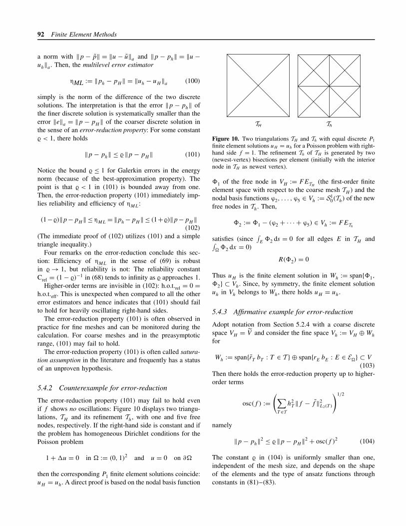
The error-reduction property (101) may fail to hold evenif f shows no oscillations: Figure 10 displays two triangu-lations, TH and its refinement Th, with one and five freenodes, respectively. If the right-hand side is constant and ifthe problem has homogeneous Dirichlet conditions for thePoisson problem
1+�u = 0 in � := (0, 1)2 and u = 0 on ∂�
then the corresponding P1 finite element solutions coincide:uH = uh. A direct proof is based on the nodal basis function
H h
Figure 10. Two triangulations TH and Th with equal discrete P1
finite element solutions uH = uh for a Poisson problem with right-hand side f = 1. The refinement Th of TH is generated by two(newest-vertex) bisections per element (initially with the interiornode in TH as newest vertex).
�1 of the free node in VH := FETH(the first-order finite
element space with respect to the coarse mesh TH ) and thenodal basis functions ϕ2, . . . , ϕ5 ∈ Vh := S1
0(Th) of the newfree nodes in Th. Then,
�2 := �1 − (ϕ2 + · · · + ϕ5) ∈ Vh := FETh
satisfies (since∫E
�2 ds = 0 for all edges E in TH and∫�
�2 dx = 0)
R(�2) = 0
Thus uH is the finite element solution in Wh := span{�1,
�2} ⊂ Vh. Since, by symmetry, the finite element solutionuh in Vh belongs to Wh, there holds uH = uh.
5.4.3 Affirmative example for error-reduction
Adopt notation from Section 5.2.4 with a coarse discretespace VH = V and consider the fine space Vh := VH ⊕Wh
for
Wh := span{rT bT : T ∈ T } ⊕ span{rE bE : E ∈ E�} ⊂ V
(103)
Then there holds the error-reduction property up to higher-order terms
osc(f ) :=(∑
T ∈Th2
T ‖f − f ‖2L2(T )
)1/2
namely
‖p − ph‖2 ≤ � ‖p − pH‖2 + osc(f )2 (104)
The constant � in (104) is uniformly smaller than one,independent of the mesh size, and depends on the shapeof the elements and the type of ansatz functions throughconstants in (81)–(83).

Finite Element Methods 93
The proof of (104) is based on the test functions wT andwE in (84) and (86) of Section 5.2.4 and
wh :=∑T∈T
wT +∑E∈E�
wE ∈ Wh ⊂ V
Utilizing (81)–(83) one can prove
‖wh‖2a ≤ C
∑T ∈T
h2T ‖rT ‖2
L2(T ) +∑E∈E�
hE ‖rE‖2L2(E)
≤ C
∑T ∈T
R(wT )+∑E∈E�
R(wE)+ osc(f )2
= C (R(wh)+ osc(f )2)
Since wh belongs to Vh and uh is the finite elementsolution with respect to Vh there holds
R(wh) = a(uh − uH , wh) ≤ ‖uh − uH‖a ‖wh‖a
The combination of the preceding inequalities yields thekey inequality
η2R,R =
∑T∈T
h2T ‖rT ‖2
L2(T ) +∑E∈E�
hE ‖rE‖2L2(E)
≤ C(‖uh − uH‖2a + osc(f )2)
This, the Galerkin orthogonality ‖u− uH‖2a = ‖u− uh‖2
a +‖uh − uH‖2
a , and the reliability of ηR show
‖u− uH‖2a ≤ CC2
rel
(‖u− uH‖2a − ‖u− uh‖2
a + osc(f )2)and so imply (104) with � = 1− C−1C−2
rel < 1.
Example 12. In the Poisson problem with P1 finite ele-ments and discrete space VH , let Wh consist of the quadraticand cubic bubble functions (80). Then (104) holds; cf. alsoExample 14 below.
Example 13. Other affirmative examples for the Poissonproblem consist of the P1 and P2 finite element spaces VH
and Vh over one regular triangulation T or of the P1 finiteelement spaces with respect to a regular triangulation TH
and its red-refinement Th. The observation that the element-bubble functions are in fact redundant is due to Dorfler andNochetto (2002).
5.4.4 Hierarchical error estimator
Given a smooth right-hand side f and based on the exampleof the previous section, the multilevel estimator (100)
is reliable and efficient up to higher-order terms. Thecostly calculation of uh, however, exclusively allows foran accurate error control of uH (and no reasonable errorcontrol for uh). Instead of (100), cheaper versions arefavored where uh is replaced by some quantity computedby a localized problem. One reliable and efficient versionis the hierarchical error estimator
ηH :=(∑
T ∈Tη2
T +∑E∈E
η2E
)1/2
(105)
where, for each T ∈ T and E ∈ E and their test functions(84) and (86),
ηT := R(wT )
‖wT ‖a
and ηE := R(wE)
‖wE‖a
(106)
(The proof of reliability and efficiency follows from (81)–(83) by the arguments from Section 5.2.4.)
Example 14. In the Poisson problem with P1 finite ele-ments and discrete space VH , let Wh consist of the quadraticand cubic bubble functions (80). Then,
ηH :=∑
T ∈T
R(bT )2
‖bT ‖2a
+∑E∈E�
R(bE)2
‖bE‖2a
1/2
(107)
is a reliable and efficient hierarchical error estimator. Withthe error-reduction property of P1 and P2 finite elementsdue to Dorfler and Nochetto (2002),
ηH :=∑
E∈E�
R(bE)2
‖bE‖2a
1/2
(108)
is reliable and efficient as well. The same is true if, foreach edge E ∈ E, bE defines a hat function of the midpointof E with respect to a red-refinement Th of TH (that is,each edge is halved and each triangle is divided into fourcongruent subtriangles; cf. Figure 15, left).
5.5 Averaging error estimators
Averaging techniques, also called (gradient) recovery esti-mators, focus on one mesh and one known low-order fluxapproximation p and the difference to a piecewise polyno-
mial q in a finite-dimensional subspace Q ⊂ L2(�;Rm×n)
of higher polynomial degrees and more restrictive continu-ity conditions than those generally satisfied by p. Averagingtechniques are universal in the sense that there is no needfor any residual or partial differential equation in order toapply them.

94 Finite Element Methods
5.5.1 Definition of averaging error estimators
The procedure consists of taking a piecewise smooth p andapproximating it by some globally continuous piecewisepolynomials (denoted by Q) of higher degree Ap. A simpleexample, frequently named after Zienkiewicz and Zhu andsometimes even called the ZZ estimator, reads as follows:For each node z ∈ N and its patch ωz let
(Ap)(z) =
∫ωz
p dx∫ωz
1 dx
∈ Rm×n (109)
be the integral mean of p over ωz. Then, define Ap byinterpolation with (conforming, i.e. globally continuous) hatfunctions ϕz, for z ∈ N,
Ap =∑z∈N
(Ap)(z) ϕz ∈ Q
Let Q = span{ϕz: z ∈ N } denote the (conforming) first-order finite element space and let ‖ · ‖ be the norm forthe fluxes. Then the averaging estimator is defined by
ηA := ‖p −Ap‖ (110)
Notice that there is a minimal version
ηM := minq∈Q
‖p − q‖ ≤ ηA (111)
The efficiency of ηM follows from a triangle inequality,namely
ηM ≤ ‖p − p‖ + ‖p − q‖ for all q ∈ Q (112)
and the fact that ‖p − p‖ = O(h) while (in all the examplesof this chapter)
minq∈Q
‖p − q‖ = h.o.t.(p) =: h.o.t.eff
This is of higher order for smooth p and efficiency followsfor η = ηM and Ceff = 1.
It turns out that ηA and ηM are very close and accurateestimators in many numerical examples; cf. Section 5.6.4below. This and the fact that the calculation of ηA is aneasy postprocessing made ηA extremely popular.
For proper treatment of Neumann boundary conditions,we refer to Carstensen and Bartels (2002) and forapplications in solid and fluid mechanics to Alberty andCarstensen (2003) and Carstensen and Funken (2001a,b)and for higher-order FEM to Bartels and Carstensen (2002).
Multigrid smoothing steps may be successfully employedas averaging procedures as proposed in Bank and Xu(2003).
5.5.2 All averaging error estimators are reliable
The first proof of reliability dates back to Rodriguez(1994a,b) and we refer to Carstensen (2004) for anoverview. A simplified reliability proof for ηM and hencefor all averaging techniques (Carstensen, Bartels and Klose,2001) is outlined in the sequel.
First let � be the L2 projection onto the first-order finiteelement space V and let q be arbitrary in Q, that is, eachof the m× n components of q is a first-order finite elementfunction in FET . The Galerkin orthogonality shows for theerror e := u− u and p := ∇u in the situation of Example 1that
‖e‖2a =
∫�
(∇u− q) · ∇(e −�e) dx
+∫
�
(q − p) · ∇(e −�e) dx
A Cauchy inequality in the latter term is combined with theH 1-stability of �, namely,
‖∇(e −�e)‖L2(�) ≤ Cstab‖∇e‖L2(�)
(For sufficient conditions for this we refer to Crouzeix andThomee (1987), Bramble, Pasciak and Steinbach (2002),Carstensen (2002, 2003b), and Carstensen and Verfurth(1999).) The H 1-stability in the second term and an inte-gration by parts in the first term on the right-hand sideshow
‖e‖2a ≤
∫�
f · (e −�e) dx +∫
�
(e −�e) · div q dx
+ Cstab‖∇e‖L2(�)‖p − q‖L2(�)
Since e −�e is L2-orthogonal onto fh := �f ∈ V ,∫�
f · (e −�e) dx
=∫
�
(f − fh) · (e −�e) dx
≤ ‖h−1T (e −�e)‖L2(�)‖hT (f −�f )‖L2(�)
Notice that, despite possible boundary layers, ‖hT (f −�f )‖L2(�) = h.o.t. is of higher order. The first-order appro-ximation property of the L2 projection,
‖h−1T (e −�e)‖L2(�) ≤ Capprox‖∇e‖L2(�)
Finite Element Methods 95
follows from the H 1-stability (cf. e.g. Carstensen andVerfurth (1999) for a proof). Similar arguments for theremaining term div q and the T-piecewise divergence oper-ator divT with div q = divT q = div T (q − p) (recall that u
is of first-order and hence �u = 0 on each element) lead to∫�
(e −�e) · div q dx
≤ Capprox‖∇e‖L2(�)‖hT divT (q − p)‖L2(�)
An inverse inequality hT ‖divT (q − p)‖L2(T ) ≤ Cinv‖q −p‖L2(T ) (cf. Section 3.4) shows∫
�
(e−�e) · div q dx≤CapproxCinv‖∇e‖L2(�)‖q−p‖L2(�)
The combination of all established estimates plus a divisionby ‖e‖a = ‖∇e‖L2(�) yield the announced reliability result
‖e‖a ≤ (Cstab + CapproxCinv)‖p − q‖L2(�) + h.o.t.
In the second step, one designs a more local approximationoperator J to substitute � as in Carstensen and Bartels(2002); the essential properties are the H 1-stability, thefirst-order approximation property, and a local form of theorthogonality condition; we omit the details.
5.5.3 Averaging error estimators and edgecontributions
There is a local equivalence of the estimators ηA from alocal averaging process (109) and the edge estimator
ηE :=∑
E∈E�
hE‖[pνE]‖2L2(E)
1/2
The observation that, with some mesh-size-independentconstant C,
C−1 ηE ≤ ηA ≤ C ηE (113)
dates back to Rodriguez (1994a) and can be found inVerfurth (1996). The proof of (113) for piecewise linearsin V is based on the equivalence of the two seminorms
�1(q) := minr∈Rm×n
‖q − r‖L2(ωz)
and
�2(q) :=∑
E∈Ez
hE‖[qνE]‖2L2(E)
1/2
for piecewise constant vector-valued functions q in Pz, theset of possible fluxes q restricted on the patch ωz of a
node z, and with the set of edges Ez := {E ∈ E : z ∈ E}.The main observation is that �1 and �2 vanish exactly forconstants functions R
m×n and hence they are norms on thequotient space Pz/R
m×n. By the equivalence of norms onany finite-dimensional space Pz/R
m×n, there holds
C−1 �1(q) ≤ �2(q) ≤ C �1(q) ∀q ∈ Pz
This is a local version of (113), which eventually implies(113) by localization and composition; we omit the details.
For triangles and tetrahedra and piecewise linear finiteelement functions, it is proved in Carstensen (2004) that
ηM ≤ ηA ≤ Cd ηM (114)
with universal constants C2 =√
10 and C3 =√
15 for 2-Dand 3-D, respectively. This equivalence holds for a largerclass of elements and (first-order) averaging operators andthen proves efficiency for ηA whereas efficiency of ηM
follows from a triangle inequality in (112).
5.6 Comparison of error bounds in benchmarkexample
This section is devoted to a numerical comparison of energyerrors and its a posteriori error estimators for an ellipticmodel problem.
5.6.1 Benchmark example
The numerical comparisons are computed for the Poissonproblem
1+�u = 0 in � and u = 0 on ∂� (115)
on the L-shaped domain � = (−1,+1)2\([0, 1]× [−1, 0])and its boundary ∂�. The first mesh T1 consists of 17free nodes and 48 elements and is obtained by, first, adecomposition of � in 12 congruent squares of size 1/2and, second, a decomposition of each of the boxes alongits two diagonals into 4 congruent triangles. The subsequentmeshes are successively red-refined (i.e. each triangle ispartitioned into 4 congruent subtriangles of Figure 15, left).This defines the (conforming) P1 finite element spaces V1 ⊂V2 ⊂ V3 ⊂ · · · ⊂ V := H 1
0 (�). The error e := u− uj ofthe finite element solution uj = u in Vj = V of dimensionN = dim(Vj ) is measured in the energy norm (the Sobolevseminorm in H 1(�))
|e|1,2 := |e|H 1(�) :=(∫
�
|De|2 dx
)1/2
= a(u− u, u+ u)1/2
=(|u|2
H 1(�)− |u|2
H 1(�)
)1/2

96 Finite Element Methods
10110−3
10−2
10−1
100
101
102 103 104 105
N
1
0.33
η/|
u|1,
2 re
sp. |
e|1,
2/|
u|1,
2
|e|1,2ηZ,AηZ,MηR,R
ηLηRC
ηR,E
ηEQ
Figure 11. Experimental results for the benchmark problem (115)with meshes T1, . . . , T6. The relative error |e|1,2/|u|1,2 and vari-ous estimators η/|u|1,2 are plotted as functions of the numberof degrees of freedom N . Both axes are in a logarithmic scal-ing such that an algebraic curve N−α is visible as a straightline with slope −α. A triangle with slope −0.33 is displayedfor comparison. A color version of this image is available athttp://www.mrw.interscience.wiley.com/ecm
(by the Galerkin orthogonality) computed with the approx-imation |u|2
H 1(�)≈ 0.21407315683398.
Figure 11 displays the computed values of |e|1,2 for asequence of uniformly refined meshes T1, T2, . . . , T6 as afunction of the number of degrees of freedom N = 17, 81,353, 1473, 6017, 24321, 97793. It is this curve that will beestimated by computable upper and lower bounds explainedin the subsequent sections where we use the fact that eachelement is a right isosceles triangle.
Notice that the two axes in Figure 11 scale logarithmi-cally such that any algebraic curve of growth α is mappedinto a straight line of slope −α. The experimental conver-gence rate is 2/3 in agreement with the (generic) singularityof the domain and resulting theoretical predictions. Moredetails can be found in Carstensen, Bartels and Klose(2001).
5.6.2 Explicit error estimators
For the benchmark problem of Section 5.6.1, the errorestimator (75) can be written in the form
ηR,R :=(∑
T∈Th2
T ‖1‖2L2(T )
)1/2
+∑
E∈E�
hE
∫E
[∂u
∂νE
]2
ds
1/2
(116)
and is reliable with Crel = 1 and h.o.t.rel = 0 (Carstensenand Funken, 2001a). Figure 11 displays ηR,R as a functionof the number of unknowns N and illustrates |e|1,2 ≤ ηR,R.
Guaranteed lower error bounds, i.e. with the efficiencyconstant Ceff, are less established and the higher-order termsh.o.t.eff usually involve ‖f − fT ‖L2(T ) for the elementwiseintegral mean fT of the right-hand side. Here, f ≡ 1 and soh.o.t.eff = 0. Following a derivation in Carstensen, Bartelsand Klose (2001), Figure 11 also displays an efficientvariant ηR,E as a lower error bound: ηR,E ≤ |e|1,2.
The guaranteed lower and upper bounds with expliciterror estimators leave a very large region for the true error.Our interpretation is that various geometries (the shape ofthe patches) lead to different constants and Crel = 1 reflectsthe worst possible situation for every patch in the currentmesh.
A more efficient reliable explicit error estimator ηR,C
from Carstensen and Funken (2001a) displayed in Figure 11requires the computation of local (patchwise) analyticaleigenvalues and hence is very expensive. However, theexplicit estimators ηR,C and ηR,E still overestimate andunderestimate the true error by a huge factor (up to 10and even more) in the simple situation of the benchmark.One conclusion is that the involved constants estimate aworst-case scenario with respect to every right-hand sideor every exact solution.
This experimental evidence supports the design of moreelaborate estimators: The stopping criterion (72) with thereliable explicit estimators may appear very cheap and easy.But the decision (72) may have too costly consequences.
5.6.3 Implicit estimators
For comparison, the two implicit estimators ηL and ηEQ
are displayed in Figure 11 as functions of N . It is stressedthat both estimators are efficient and reliable (Carstensenand Funken, 1999/00)
|e|1,2 ≤ ηL ≤ 2.37 |e|1,2
The practical performance of ηL and ηEQ in Figure 11 iscomparable and in fact is much sharper than that of ηR,E
and ηR,R.
5.6.4 Averaging estimator
The averaging estimators ηA and ηM are as well displayedin Figure 11 as a function of N . Here, ηM is efficient up tohigher-order terms (since the exact solution u ∈ H 5/3−ε(�)
is singular, this is not really guaranteed) while its reliabilityis open, i.e. the corresponding constants have not beencomputed. Nevertheless, the behavior of ηA and ηM isexclusively seen here from an experimental point of view.
Finite Element Methods 97
The striking numerical result is an amazing high accuracy ofηM ≈ ηA as an empirical guess of |e|1,2. If we took Crel intoaccount, this effect would be destroyed: The high accuracyis an empirical observation in this example (and possiblymany others) but does not yield an accurate guaranteederror bound.
5.6.5 Adapted meshes
The benchmark in Figure 11 is based on a sequence ofuniform meshes and hence results in an experimental con-vergence rate 2/3 according to the corner singularity ofthis example. Adaptive mesh-refining algorithms, describedbelow in more detail, are empirically studied also inCarstensen, Bartels and Klose (2001). The observations canbe summarized as follows: The quality of the estimators andtheir relative accuracy is similar to what is displayed inFigure 11 even though the convergence rates are optimallyimproved to one.
5.7 Goal-oriented error estimators
This section provides a brief introduction to goal-orientederror control.
5.7.1 Goal functionals
Given the Sobolev space V = H 10 (�) with a finite-dimen-
sional subspace V ⊂ V , a bounded and V -elliptic bilinearform a : V × V → R, a bounded linear form F : V → R,there exists an exact solution u ∈ V and a discrete solutionu ∈ V of
a(u, v) = F(v) ∀v ∈ V and a(u, v) = F(v) ∀v ∈ V
(117)
The previous sections concern estimations of the errore := u− u in the energy norm, equivalent to the Sobolevnorm in V . Other norms are certainly of some interest aswell as the error with respect to a certain goal functional.The latter is some given bounded and linear functionalJ : V → R with respect to which one aims to monitor theerror, that is, one wants to find computable lower and upperbounds for the (unknown) quantity
|J (u)− J (u)| = |J (e)|Typical examples of goal functionals are described by L2functions, for example,
J (v) =∫
�
� v dx ∀v ∈ V
for a given � ∈ L2(�) or as contour integrals.
In many cases, the main interest is on a point value andthen J (v) is given by a mollification � of a singular measurein order to guarantee the boundedness of J : V → R.
5.7.2 Duality technique
To bound or approximate J (e) one considers the dualproblem
a(v, z) = J (v) ∀v ∈ V (118)
with exact solution z ∈ V (guaranteed by the Lax–Milgramlemma) and the discrete solution z ∈ V of
a(v, z) = J (v) ∀v ∈ V
Set f := z− z. On the basis of the Galerkin orthogonalitya(e, z) = 0 one infers
J (e) = a(e, z) = a(e, z− z) = a(e, f ) (119)
As a result of (119) and the boundedness of a one obtainsthe a posteriori estimate
|J (e)| ≤ ‖a‖ ‖e‖V ‖f ‖V ≤ ‖a‖ηuηz
Indeed, utilizing the primal and dual residual Ru and Rz inV ∗, defined by
Ru := F − a(u, ·) and Rz := J − a(·, z)
computable upper error bounds for ‖e‖V ≤ ηu and ‖f ‖V ≤ηz can be found by the arguments of the energy error esti-mators of the previous sections. This yields a computableupper error bound ‖a‖ηuηz for |J (e)| which is global,that is, the interaction of e and f is not reflected. Onemight therefore speculate that the upper bound is often toocoarse and inappropriate for goal-oriented adaptive meshrefinement.
5.7.3 Upper and lower bounds of J (e)
Throughout the rest of this section, let the bilinear form a besymmetric and positive definite; hence a scalar product withinduced norm ‖ · ‖a . Then, the parallelogram rule shows
2 J (e) = 2 a(e, f ) = ‖e + f ‖2a − ‖e‖2
a − ‖f ‖2a
This right-hand side can be written in terms of residuals,in the spirit of (70), namely, ‖e‖a = ‖Resu‖V ∗ , ‖f ‖a =‖Resz‖V ∗ , and
‖e + f ‖a =‖Resu+z‖V ∗ for Resu+z :=F + J − a(u+ z, ·)= Resu + Resz ∈ V ∗

98 Finite Element Methods
Therefore, the estimation of J (e) is reduced to the computa-tion of lower and upper error bounds for the three residualsResu, Resz, and Resu+z with respect to the energy norm.This illustrates that the energy error estimation techniquesof the previous sections may be employed for goal-orientederror control.
For more details and examples of a refined estimation seeAinsworth and Oden (2000) and Babuska and Strouboulis(2001).
5.7.4 Computing an approximation to J (e)
An immediate consequence of (119) is
J (e) = R(z)
and hence J (e) is easily computed once the dual solutionz of (118) is known or at least approximated to suffi-cient accuracy. An upper error bound for |J (e)| = |R(z)|is obtained following the methodology of Becker and Ran-nacher (1996, 2001) and Bangerth and Rannacher (2003).
To outline this methodology, consider the residual rep-resentation formula (73) following the notation of Sec-tion 5.2.1. Suppose that z ∈ H 2(�) (e.g. for a H 2 regulardual problem) and let Iz denote the nodal interpolant in thelowest-order finite element space V . With some interpola-tion constant CI > 0, there holds, for any element T ∈ T,
h−2T ‖z− Iz‖L2(T ) + h
−3/2T ‖z− Iz‖L2(∂T ) ≤ CI |z|H 2(T )
The combination of this with (73) shows
J (e) = Res(z − Iz)
=∑T ∈T
∫T
rT · (z − Iz) dx −∑E∈E
∫E
rE · (z − Iz) ds
≤∑T∈T
(‖rT ‖L2(T ) ‖z− Iz‖L2(T )
+ ‖rE‖L2(∂T ) ‖z− Iz‖L2(∂T )
)≤∑T∈T
CI
(h2
T ‖rT ‖L2(T ) + h3/2T ‖rE‖L2(∂T )
)|z|H 2(T )
The influence of the goal functional in this upper boundis through the unknown H 2 seminorm |z|H 2(T ), which isto be replaced by some discrete analog based on a com-puted approximation zh. The justification of some substitute|D2
hzh|L2(T ) (postprocessed with some averaging technique)for |z|H 2(T ) is through striking numerical evidence; we referto Becker and Rannacher (2001) and Bangerth and Ran-nacher (2003) for details and numerical experiments.
6 LOCAL MESH REFINEMENT
This section is devoted to the mesh-design task in the finiteelement method based on a priori and a posteriori infor-mation. Examples of the former type are graded meshesor geometric meshes with an a priori choice of refinementtoward corner singularities briefly mentioned in Section 6.1.Examples of the latter type are adaptive algorithms for auto-matic mesh refinement (or mesh coarsening) strategies witha successive call of the steps
SOLVE⇒ESTIMATE⇒MARK⇒REFINE/COARSEN
Given the current triangulation, one has to compute thefinite element solution in step SOLVE; cf. Section 7.8 fora MATLAB realization of that. The accuracy of this finiteelement approximation is checked in the step ESTIMATE.On the basis of the refinement indicators of Section 6.2the step MARK identifies the elements, edges or patches inthe current mesh in need of refinement (or coarsening). Thenew data structure is generated in step REFINE/COARSENwhere a partition is given and a closure algorithm com-putes a triangulation described in Section 6.3. The conver-gence and optimality of the adaptive algorithm is discussedin Section 6.4. Brief remarks on coarsening strategies inSection 6.5 conclude the section.
6.1 A priori mesh design
The singularities of the exact solution of the Laplace equa-tion on domains with corners (cf. Figure 1) are reasonablywell understood and motivate the (possibly anisotropic)mesh refinement toward vertices or edges. This sectionaims a short introduction for two-dimensional P1 finiteelements – Chapter 3, this Volume, will report on three-dimensional examples.
Given a polygonal domain with a coarse triangulationinto triangles (which specify the geometry), macro ele-ments can be used to fill the domain with graded meshes.Figure 12(a) displays a macro element described in thesequel while Figure 12(b) illustrates the resulting fine meshfor an L-shaped domain.
The description is restricted to the geometry on thereference element Tref with vertices (0, 0), (1, 0), and (0, 1)
of Figure 12(a). The general situation is then obtained byan affine transformation illustrated in Figure 12(b). Themacro element Tref is generated as follows: Given a gradingparameter β > 0 for a grading function g(t) = tβ, andgiven a natural number N , set ξj := g(j/N) and drawline segments aligned to the antidiagonal through (0, ξj )
and (ξj , 0) for j = 0, 1, . . . , N . Each of these segments

Finite Element Methods 99
ξ1ξ2
ξ2
ξ3
ξ4
ξ1 ξ4ξ3(a)
1 0.8 0.6 0.4 0.2 0 0.2 0.4 0.6 0.8 11
0.8
0.6
0.4
0.2
0
0.2
0.4
0.6
0.8
1
(b)
Figure 12. (a) Reference domain Tref with graded mesh for β =3/2 and N = 4. (b) Graded mesh on L-shaped domain withrefinement toward origin and uniform refinement far away fromthe origin. Notice that the outer boundaries of the macro elementsshow a uniform distribution and so match each other in one globalregular triangulation.
is divided into j uniform edges and so define the setof nodes (0, 0) and ξj /j (j − k, k) for k = 0, . . . , j andj = 1, . . . , N . The elements are then given by the verticesξj /j (j − k, k) and ξj /j (j − k − 1, k + 1) aligned with theantidiagonal and the vertex ξj−1/(j − 1) (j − k − 1, k) onthe finer and ξj+1/(j + 1) (j − k, k + 1) on the coarserneighboring segment, respectively. The finest element isconv{(0, 0), (0, ξ1), (ξ1, 0)} of diameter
√(2) g(1/N) ≈
N−β.Figure 12(b) displays a triangulation of the L-shaped
domain with a refinement toward the origin designed bya union of transformed macro elements with β = 3/2 andN = 7. The other vertices of the L-shaped domain yieldhigher singularities, which are not important for the first-order Courant finite element.
The geometric mesh depicted in Figure 13 yields a finerrefinement toward some corners of the polygonal domain.Given a parameter β > 0 in this type of triangulation,
(a) (b)
Figure 13. (a) Reference domain Tref with geometric mesh forparameter β = 1/2 and N = 4. This mesh can also be gener-ated by an adaptive red–green–blue refinement of Section 6.3.(b) Illustration of the closure algorithm. The refinement triangula-tion with 50 element domains is obtained from the mesh (a) with18 element domains by marking one edge (namely the secondalong the antidiagonal) in the mesh (a).
the nodes ξ0 := 0 and ξj := βN−j for j = 1, . . . , N defineantidiagonals through (ξj , 0) and (0, ξj ), which are in turnbisected. For such a triangulation, the polynomial degreespT on each triangle T are distributed as follows: pT =1 for the two triangles T with vertex (0, 0) and pT =j + 2 for the four elements in the convex quadrilateralwith the vertices (ξj , 0), (0, ξj ), (ξj+1, 0), and (0, ξj+1)
for j = 0, . . . , N − 1. Figure 14 compares experimentalconvergence rates of the error in H−1-seminorm |e|H 1 forvarious graded meshes for the P1 finite element method,the p-and hp-finite element method, and for the adaptivealgorithm of Section 6.4. The P1 finite element methodon graded meshes with β = 3/2, β = 2 and h-adaptivityrecover optimality in the convergence rate as opposite to theuniform refinement (β = 1), leading only to a sub-optimalconvergence due to the corner singularity. The hp-finiteelement method performs better convergence rate comparedto the p-finite element method.
Tensor product meshes are more appropriate for smallervalues of β; the one-dimensional model analysis of Babuskaand Guo (1986) suggests β = (2)1/2 − 1 ≈ 0.171573.
6.2 Adaptive mesh-refining algorithms
The automatic mesh refinement for regular triangulationscalled MARK and REFINE/COARSEN frequently consistsof three stages:
(i) the marking of elements or edges for refinement (orcoarsening);
(ii) the closure algorithm to ensure that the resultingtriangulation is (or remains) regular;
(iii) the refinement itself, i.e. the change of the underlyingdata structures.
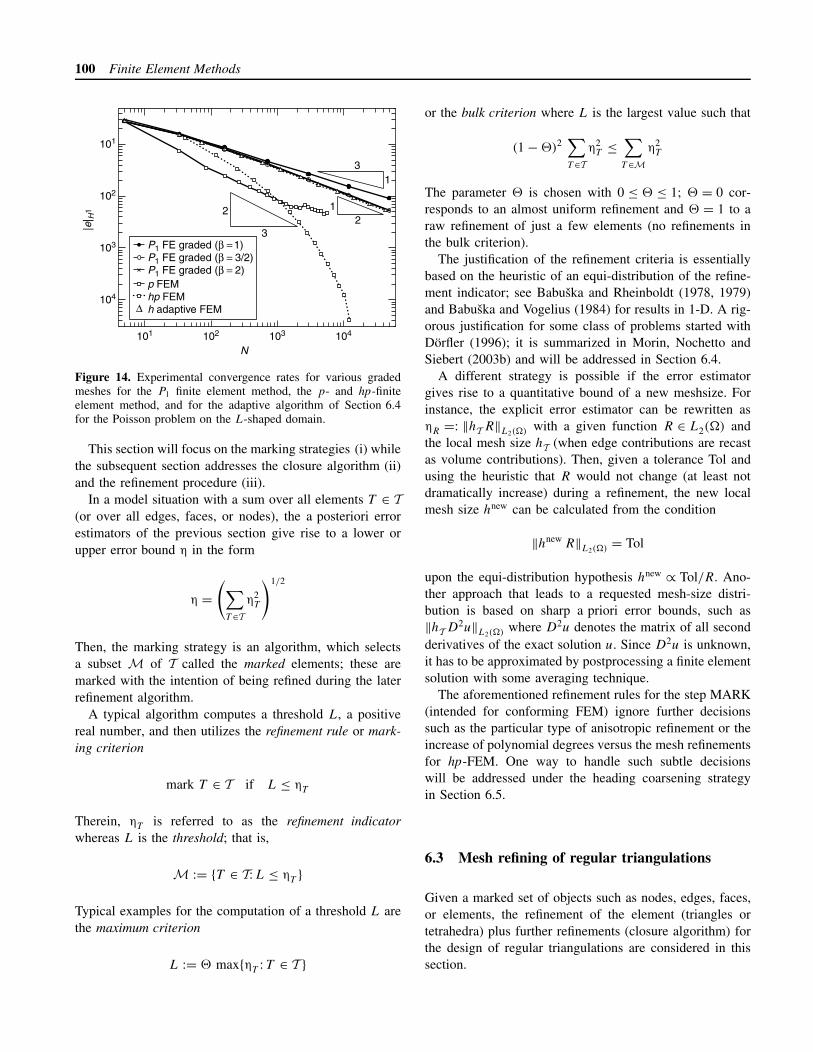
100 Finite Element Methods
101 102 103 104
104
103
102
101
N
|e| H
1
31
21
3
2
P1 FE graded (β = 1)P1 FE graded (β = 3/2)P1 FE graded (β = 2)p FEMhp FEMh adaptive FEM∆
Figure 14. Experimental convergence rates for various gradedmeshes for the P1 finite element method, the p- and hp-finiteelement method, and for the adaptive algorithm of Section 6.4for the Poisson problem on the L-shaped domain.
This section will focus on the marking strategies (i) whilethe subsequent section addresses the closure algorithm (ii)and the refinement procedure (iii).
In a model situation with a sum over all elements T ∈ T(or over all edges, faces, or nodes), the a posteriori errorestimators of the previous section give rise to a lower orupper error bound η in the form
η =(∑
T ∈Tη2
T
)1/2
Then, the marking strategy is an algorithm, which selectsa subset M of T called the marked elements; these aremarked with the intention of being refined during the laterrefinement algorithm.
A typical algorithm computes a threshold L, a positivereal number, and then utilizes the refinement rule or mark-ing criterion
mark T ∈ T if L ≤ ηT
Therein, ηT is referred to as the refinement indicatorwhereas L is the threshold; that is,
M := {T ∈ T: L ≤ ηT }
Typical examples for the computation of a threshold L arethe maximum criterion
L := � max{ηT : T ∈ T }
or the bulk criterion where L is the largest value such that
(1−�)2∑T ∈T
η2T ≤
∑T ∈M
η2T
The parameter � is chosen with 0 ≤ � ≤ 1; � = 0 cor-responds to an almost uniform refinement and � = 1 to araw refinement of just a few elements (no refinements inthe bulk criterion).
The justification of the refinement criteria is essentiallybased on the heuristic of an equi-distribution of the refine-ment indicator; see Babuska and Rheinboldt (1978, 1979)and Babuska and Vogelius (1984) for results in 1-D. A rig-orous justification for some class of problems started withDorfler (1996); it is summarized in Morin, Nochetto andSiebert (2003b) and will be addressed in Section 6.4.
A different strategy is possible if the error estimatorgives rise to a quantitative bound of a new meshsize. Forinstance, the explicit error estimator can be rewritten asηR =: ‖hT R‖L2(�) with a given function R ∈ L2(�) andthe local mesh size hT (when edge contributions are recastas volume contributions). Then, given a tolerance Tol andusing the heuristic that R would not change (at least notdramatically increase) during a refinement, the new localmesh size hnew can be calculated from the condition
‖hnew R‖L2(�) = Tol
upon the equi-distribution hypothesis hnew ∝ Tol/R. Ano-ther approach that leads to a requested mesh-size distri-bution is based on sharp a priori error bounds, such as‖hT D2u‖L2(�) where D2u denotes the matrix of all secondderivatives of the exact solution u. Since D2u is unknown,it has to be approximated by postprocessing a finite elementsolution with some averaging technique.
The aforementioned refinement rules for the step MARK(intended for conforming FEM) ignore further decisionssuch as the particular type of anisotropic refinement or theincrease of polynomial degrees versus the mesh refinementsfor hp-FEM. One way to handle such subtle decisionswill be addressed under the heading coarsening strategyin Section 6.5.
6.3 Mesh refining of regular triangulations
Given a marked set of objects such as nodes, edges, faces,or elements, the refinement of the element (triangles ortetrahedra) plus further refinements (closure algorithm) forthe design of regular triangulations are considered in thissection.
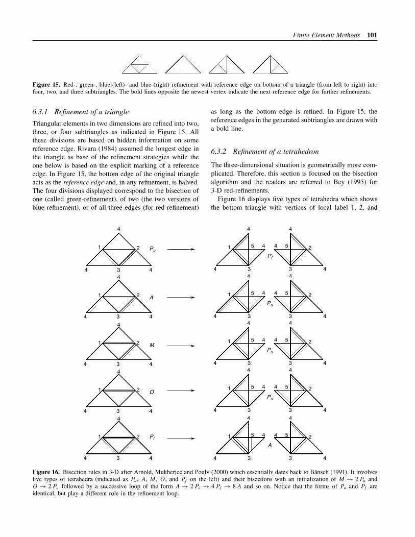
Finite Element Methods 101
Figure 15. Red-, green-, blue-(left)- and blue-(right) refinement with reference edge on bottom of a triangle (from left to right) intofour, two, and three subtriangles. The bold lines opposite the newest vertex indicate the next reference edge for further refinements.
6.3.1 Refinement of a triangle
Triangular elements in two dimensions are refined into two,three, or four subtriangles as indicated in Figure 15. Allthese divisions are based on hidden information on somereference edge. Rivara (1984) assumed the longest edge inthe triangle as base of the refinement strategies while theone below is based on the explicit marking of a referenceedge. In Figure 15, the bottom edge of the original triangleacts as the reference edge and, in any refinement, is halved.The four divisions displayed correspond to the bisection ofone (called green-refinement), of two (the two versions ofblue-refinement), or of all three edges (for red-refinement)
as long as the bottom edge is refined. In Figure 15, thereference edges in the generated subtriangles are drawn witha bold line.
6.3.2 Refinement of a tetrahedron
The three-dimensional situation is geometrically more com-plicated. Therefore, this section is focused on the bisectionalgorithm and the readers are referred to Bey (1995) for3-D red-refinements.
Figure 16 displays five types of tetrahedra which showsthe bottom triangle with vertices of local label 1, 2, and
1
4 4
4
4 3 3 4
1 5 4 4
4
5 2
4
Pu
A
Pf
4 3 3 4
1 5 4 4
4
5 2
4
Pu
4 3 3 4
1 5 4 4
4
5 2
4
Pu
4 3 3 4
1 5 4 4
4
5 2
4
Pu
4 3 3 4
1 5 4 4
4
5 2
4
A
2
3
1
4 4
4
2
3
M1
4 4
4
2
3
O1
4 4
4
2
3
Pf1
4 4
4
2
3
Figure 16. Bisection rules in 3-D after Arnold, Mukherjee and Pouly (2000) which essentially dates back to Bansch (1991). It involvesfive types of tetrahedra (indicated as Pu, A, M , O, and Pf on the left) and their bisections with an initialization of M → 2 Pu andO → 2 Pu followed by a successive loop of the form A → 2 Pu → 4 Pf → 8 A and so on. Notice that the forms of Pu and Pf areidentical, but play a different role in the refinement loop.
102 Finite Element Methods
3 while the remaining three faces with the vertex label 4are drawn in the same plane as the bottom face; hence, thesame number 4 for the top vertex is visible at the end-pointsof the three outer subtriangles.
Each triangular face has a reference edge and (at least)one edge is a reference edge of the two neighboring facesand that determines the vertices with local numbers 1 and 2.In the language of Arnold, Mukherjee and Pouly (2000), thefive appearing types are called Pu, A, M , O, and Pf . Thebisection of the edges between the vertices number 1 and 2with the new vertex number 5 are indicated in Figure 16.
It is an important property of the inherited referenceedges that the edges of each element K in the originalregular triangulation T are refined in a cyclic way such thatfour consecutive bisections inside K are necessary before anew vertex is generated, which is not the midpoint of someedge of K .
6.3.3 Closure algorithms
The bisection of some set of marked elements does notalways lead to a regular triangulation – the new verticesmay be hanging nodes for the neighboring elements. Furtherrefinements are necessary to make those nodes regular. Thedefault procedure within the class of bisection algorithmsis to work on a set of marked elements M(k).
Closure Algorithm for Bisection. Input a regular trian-gulation T (0) := T and an initial subset M(0) :=M ⊂ T (0)
of marked elements, set Z = ∅ and k := 0.While M(k) = ∅ repeat (i)–(iv):
(i) choose some element K in M(k) with reference edgeE and initiate its midpoint zK as new vertex, setZ := Z ∪ {zK};
(ii) bisect E and divide K into K+ and K− and setT (k+1) := {K+, K−} ∪ (T (k) \ {K});
(iii) find all elements T1, . . . , TmK∈ T (k+1) with han-
ging node z ∈ Z (if any) and set M(k+1) :={T1, . . . , TmK
} ∪ (M(k) \ {K});(iv) update k := k + 1 and go to (i).
Output a refined triangulation T (k).
According to step (iii) of the closure algorithm, any ter-mination leads to a regular triangulation T (k). The remainingessential detail is to guarantee that there will always occur atermination via M(k) = ∅ for some k. In the newest-vertexbisection, for instance, the reference edges are inherited insuch a way that any element K ∈ T, the initial regular tri-angulation, is refined only by subdivisions which, at most,halve each edge of K . Since the closure algorithm onlyhalves some edge in T and prohibits any further refinements,
any intermediate (irregular) T (k) remains coarser than orequal to some regular uniform refinement T of T. This is themain argument to prove that the closure algorithm cannotrefine forever and stops after a finite number of steps.
Figure 13(b) shows an example where, given the initialmesh of Figure 13(a), only one edge, namely the second onthe diagonal, is marked for refinement and the remainingrefinement is induced by the closure algorithm. Neverthe-less, the number of new elements can be bounded in termsof the initial triangulation and the number of marked ele-ments (Binev, Dahmen and DeVore, 2004).
The closure algorithm for the red–green–blue refinementin 2-D is simpler when the focus is on marking of edges.One main ingredient is that each triangle K is assigneda reference edge E(K). If we are given a set of markedelements, let M denote the set of corresponding assignedreference edges.
Closure Algorithm for Red–Green–Blue Refinement.Input a regular triangulation T with a set of edges E andan initial subset M ⊂ E of marked edges, set k := 0 andM(0) := N (0) :=M.
While N(k) = ∅ repeat (i)–(iv):
(i) choose some edge E in N (k) and let T± ∈ T denotethe (at most) two triangles that share the edge E ⊂∂T±;
(ii) set M(k+1) :=M(k) ∪ {E+, E−} with the referenceedge E± := E(T±) of T±;
(iii) if M(k+1) =M(k) set N(k+1) := N(k) \ {E} else setN(k+1) := (N(k) ∪ {E+, E−}) \ {E};
(iv) update k := k + 1 and go to (i).
Bisect the marked edges {E ∈M(k) : E ⊂ ∂T } of eachelement T ∈ T and refine T by one of the red–green–bluerefinement rules to generate elementwise a partition T .
Output the regular triangulation T .
The closure algorithm for red–green–blue refinementterminates as N(k) is decreasing and M(k) is increasingand outputs a set M :=M(k) of marked edges with thefollowing closure property: Any element T ∈ T with anedge in M satisfies E(T ) ∈M, i.e. if T is marked, thenat least its reference edge will be halved. This propertyallows the application of one properly chosen refinementof Figure 15 and leads to a regular triangulation.
The reference edge E(K) in the closure algorithm isassigned to each element K of the initial triangulationand then is inherited according to the rules of Figure 15.For newest-vertex bisection, each triangle with vertices ofglobal numbers j , k, and � has the reference edge oppositeto the vertex number max{j, k, �}.
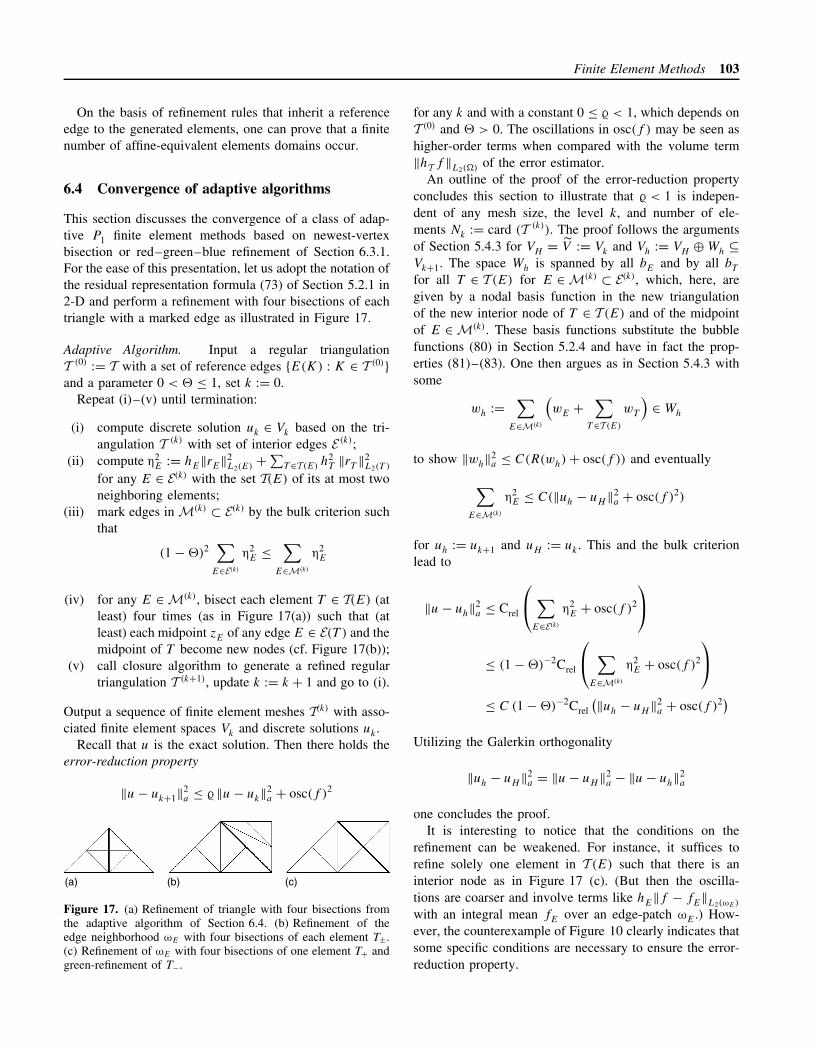
Finite Element Methods 103
On the basis of refinement rules that inherit a referenceedge to the generated elements, one can prove that a finitenumber of affine-equivalent elements domains occur.
6.4 Convergence of adaptive algorithms
This section discusses the convergence of a class of adap-tive P1 finite element methods based on newest-vertexbisection or red–green–blue refinement of Section 6.3.1.For the ease of this presentation, let us adopt the notation ofthe residual representation formula (73) of Section 5.2.1 in2-D and perform a refinement with four bisections of eachtriangle with a marked edge as illustrated in Figure 17.
Adaptive Algorithm. Input a regular triangulationT (0) := T with a set of reference edges {E(K) : K ∈ T (0)}and a parameter 0 < � ≤ 1, set k := 0.
Repeat (i)–(v) until termination:
(i) compute discrete solution uk ∈ Vk based on the tri-angulation T (k) with set of interior edges E (k);
(ii) compute η2E := hE‖rE‖2
L2(E) +∑
T ∈T (E) h2T ‖rT ‖2
L2(T )
for any E ∈ E(k) with the set T(E) of its at most twoneighboring elements;
(iii) mark edges in M(k) ⊂ E(k) by the bulk criterion suchthat
(1−�)2∑
E∈E(k)
η2E ≤
∑E∈M(k)
η2E
(iv) for any E ∈M(k), bisect each element T ∈ T(E) (atleast) four times (as in Figure 17(a)) such that (atleast) each midpoint zE of any edge E ∈ E(T ) and themidpoint of T become new nodes (cf. Figure 17(b));
(v) call closure algorithm to generate a refined regulartriangulation T (k+1), update k := k + 1 and go to (i).
Output a sequence of finite element meshes T(k) with asso-ciated finite element spaces Vk and discrete solutions uk .
Recall that u is the exact solution. Then there holds theerror-reduction property
‖u− uk+1‖2a ≤ � ‖u− uk‖2
a + osc(f )2
(a) (b) (c)
Figure 17. (a) Refinement of triangle with four bisections fromthe adaptive algorithm of Section 6.4. (b) Refinement of theedge neighborhood ωE with four bisections of each element T±.(c) Refinement of ωE with four bisections of one element T+ andgreen-refinement of T−.
for any k and with a constant 0 ≤ � < 1, which depends onT (0) and � > 0. The oscillations in osc(f ) may be seen ashigher-order terms when compared with the volume term‖hT f ‖L2(�) of the error estimator.
An outline of the proof of the error-reduction propertyconcludes this section to illustrate that � < 1 is indepen-dent of any mesh size, the level k, and number of ele-ments Nk := card (T (k)). The proof follows the argumentsof Section 5.4.3 for VH = V := Vk and Vh := VH ⊕Wh ⊆Vk+1. The space Wh is spanned by all bE and by all bT
for all T ∈ T (E) for E ∈M(k) ⊂ E(k), which, here, aregiven by a nodal basis function in the new triangulationof the new interior node of T ∈ T (E) and of the midpointof E ∈M(k). These basis functions substitute the bubblefunctions (80) in Section 5.2.4 and have in fact the prop-erties (81)–(83). One then argues as in Section 5.4.3 withsome
wh :=∑
E∈M(k)
(wE +
∑T ∈T (E)
wT
)∈ Wh
to show ‖wh‖2a ≤ C(R(wh)+ osc(f )) and eventually
∑E∈M(k)
η2E ≤ C(‖uh − uH‖2
a + osc(f )2)
for uh := uk+1 and uH := uk . This and the bulk criterionlead to
‖u− uh‖2a ≤ Crel
∑E∈E(k)
η2E + osc(f )2
≤ (1−�)−2Crel
∑E∈M(k)
η2E + osc(f )2
≤ C (1−�)−2Crel
(‖uh − uH‖2a + osc(f )2)
Utilizing the Galerkin orthogonality
‖uh − uH‖2a = ‖u− uH‖2
a − ‖u− uh‖2a
one concludes the proof.It is interesting to notice that the conditions on the
refinement can be weakened. For instance, it suffices torefine solely one element in T (E) such that there is aninterior node as in Figure 17 (c). (But then the oscilla-tions are coarser and involve terms like hE‖f − fE‖L2(ωE)
with an integral mean fE over an edge-patch ωE .) How-ever, the counterexample of Figure 10 clearly indicates thatsome specific conditions are necessary to ensure the error-reduction property.

104 Finite Element Methods
6.5 Coarsening
The constructive task in approximation theory is the designof effective approximations of a given function u. Replac-ing the unknown u by a very accurate known approximation(e.g. obtained by some overkill computation) of it, one mayemploy all the approximation techniques available and findan efficient representation in terms of an adapted finite ele-ment space, i.e. in terms of an underlying adapted meshand/or an adapted distribution of polynomial degrees.
The input of this coarsening step consists, for instance, ofa given triangulation Tk and a given finite element solutionuk and some much more accurate approximation uk . Then,the difference
ηk := ‖uk − uk‖a
is an error estimator as accurate as ‖u− uk‖a (reliabilityand efficiency is proved by a triangle inequality). Moreover,one might use ηT = |uk − uk|H 1(T ) as a local refinementindicator in the setting of the benchmark example.
Moreover, many decisions of the mesh design (e.g.choice of anisotropic elements, choice of polynomial deg-ree, etc.) can be based on the explicit availability of uk .
One single coarsening step is certainly pointless, forthe reference solution uk is known and regarded as veryaccurate (and so there is no demand for further work).On the other hand, a cascade of coarsening steps requiresin each step, a high accuracy relative to the precision ofthat level and hence a restricted accuracy. A schematicdescription of this procedure reads as follows:
Coarsening Algorithm for Adaptive Mesh Design. Inputa finite element space V0 with a finite element solution u0,set k := 0.
Repeat (i)–(iv) until termination:
(i) design a super space Vk of Vk by uniform red-refinements plus uniform increase of all the polyno-mial degrees;
(ii) compute accurate finite element solution uk withrespect to Vk;
(iii) coarsen Vk based on given uk and design a new finiteelement space Vk+1;
(iv) update k := k + 1 and go to (i).
The paper of Binev, Dahmen and DeVore (2004) presentsa realization of this algorithm with an adaptive algorithmon stage (i) and then proves that the convergence rate ofthe overall procedure is optimal with respect to the energyerror as a function of the number of degrees of freedom.
An automatic version of the coarsening strategy is calledthe hp-adaptive finite element method in Demkowicz (2003)
for higher-order polynomials adaptivity. This involves algo-rithms for the determination of edges that will be refinedand of their polynomial degrees.
7 OTHER ASPECTS
In this section, we discuss briefly several topics in finiteelement methodology. Some of the discussions involve theSobolev space Wk
p (�) (1 ≤ p ≤ ∞), which is the space offunctions in Lp(�) whose weak derivatives up to order k
also belong to Lp(�), with the norm
‖v‖Wkp (�) =
( ∑|α|≤k
∥∥∥∥∂αv
∂xα
∥∥∥∥Lp(�)
)1/p
for 1 ≤ p < ∞ and
‖v‖Wk∞(�) = max|α|≤k
∥∥∥∥(∂αv
∂xα
)∥∥∥∥L∞(�)
For 1≤p<∞, the seminorm(∑
|α|=k ‖(∂αv/∂xα)‖Lp(�)
)1/p
will be denoted by |v|Wkp (�), and the seminorm
max|α|=k ‖(∂αv/∂xα)‖L∞(�) will be denoted by |v|Wk∞(�).
7.1 Nonsymmetric/indefinite problems
The results in Section 4 can be extended to the casewhere the bilinear form a(·, ·) in the weak problem (1)is nonsymmetric and/or indefinite due to lower order termsin the partial differential equation. We assume that a(·, ·) isbounded (cf. (2)) on the closed subspace V of the Sobolevspace Hm(�) and replace (3) by the condition that
a(v, v)+ L‖v‖2L2(�) ≥ C3‖v‖2
Hm(�) ∀ v ∈ V (120)
where L is a positive constant.
Example 15. Let a(·, ·) be defined by
a(v1, v2) =∫
�
∇v1 · ∇v2 dx +d∑
j=1
∫�
bj (x)∂v1
∂xj
v2 dx
+∫
�
c(x)v1 v2 dx (121)
for all v1, v2 ∈ H 1(�), where bj (x) (1 ≤ j ≤ d), c(x) ∈L∞(�). If we take V = {v ∈ H 1(�) : v
∣∣�= 0} and F is
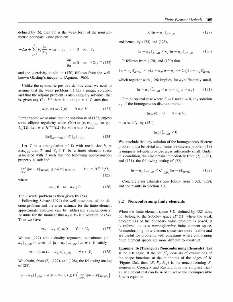
Finite Element Methods 105
defined by (6), then (1) is the weak form of the nonsym-metric boundary value problem
−�u+d∑
j=1
bj
∂u
∂xj
+ cu = f, u = 0 on �,
∂u
∂n= 0 on ∂� \ � (122)
and the coercivity condition (120) follows from the well-known Garding’s inequality (Agmon, 1965).
Unlike the symmetric positive definite case, we need toassume that the weak problem (1) has a unique solution,and that the adjoint problem is also uniquely solvable, thatis, given any G ∈ V ∗ there is a unique w ∈ V such that
a(v, w) = G(v) ∀ v ∈ V (123)
Furthermore, we assume that the solution w of (123) enjoyssome elliptic regularity when G(v) = (g, v)L2(�) for g ∈L2(�), i.e., w ∈ Hm+α(�) for some α > 0 and
‖w‖Hm+α(�) ≤ C‖g‖L2(�) (124)
Let T be a triangulation of � with mesh size hT =maxT ∈T diam T and VT ⊂ V be a finite element spaceassociated with T such that the following approximationproperty is satisfied:
infv∈VT
‖w − v‖Hm(�) ≤ εT‖w‖Hm+α(�) ∀w ∈ Hm+α(�)
(125)
where
εT ↓ 0 as hT ↓ 0 (126)
The discrete problem is then given by (54).Following Schatz (1974) the well-posedness of the dis-
crete problem and the error estimate for the finite elementapproximate solution can be addressed simultaneously.Assume for the moment that uT ∈ VT is a solution of (54).Then we have
a(u− uT, v) = 0 ∀ v ∈ VT (127)
We use (127) and a duality argument to estimate ‖u−uT ‖L2(�) in terms of ‖u− uT ‖Hm(�). Let w ∈ V satisfy
a(v, w) = (u− uT, v)L2(�) ∀ v ∈ VT (128)
We obtain, from (2), (127), and (128), the following analogof (24):
‖u− uT ‖2L2(�) = a(u− uT, w) ≤ C
(infv∈VT
‖w − v‖Hm(�)
)
× ‖u− uT ‖Hm(�) (129)
and hence, by (124) and (125),
‖u− uT ‖L2(�) ≤ εT ‖u− uT ‖Hm(�) (130)
It follows from (120) and (130) that
‖u− uT ‖2Hm(�) ≤ a(u− uT, u− uT )+ Cε2
T‖u− uT ‖2Hm(�)
which together with (126) implies, for hT sufficiently small,
‖u− uT ‖2Hm(�) ≤ a(u− uT, u− uT ) (131)
For the special case where F = 0 and u = 0, any solutionuT of the homogeneous discrete problem
a(uT, v) = 0 ∀ v ∈ VT
must satisfy, by (131),
‖uT ‖2Hm(�) ≤ 0
We conclude that any solution of the homogeneous discreteproblem must be trivial and hence the discrete problem (19)is uniquely solvable provided hT is sufficiently small. Underthis condition, we also obtain immediately from (2), (127),and (131), the following analog of (22):
‖u− uT ‖Hm(�) ≤ C infv∈VT
‖u− v‖Hm(�) (132)
Concrete error estimates now follow from (132), (129),and the results in Section 3.3.
7.2 Nonconforming finite elements
When the finite element space FET defined by (32) doesnot belong to the Sobolev space Hm(�) where the weakproblem (1) of the boundary value problem is posed, itis referred to as a nonconforming finite element space.Nonconforming finite element spaces are more flexible andare useful for problems with constrains where conformingfinite element spaces are more difficult to construct.
Example 16 (Triangular Nonconforming Elements) LetK be a triangle. If the set NK consists of evaluations ofthe shape functions at the midpoints of the edges of K
(Figure 18a), then (K, P1,NK) is the nonconforming P1element of Crouzeix and Raviart. It is the simplest trian-gular element that can be used to solve the incompressibleStokes equation.
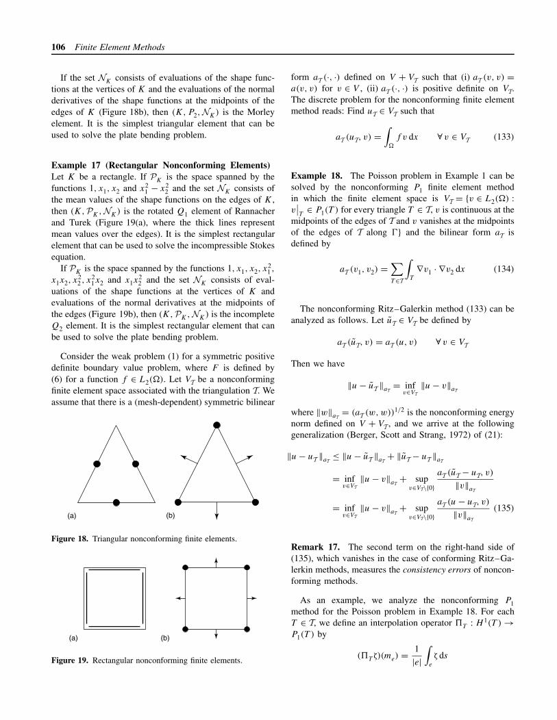
106 Finite Element Methods
If the set NK consists of evaluations of the shape func-tions at the vertices of K and the evaluations of the normalderivatives of the shape functions at the midpoints of theedges of K (Figure 18b), then (K, P2,NK) is the Morleyelement. It is the simplest triangular element that can beused to solve the plate bending problem.
Example 17 (Rectangular Nonconforming Elements)Let K be a rectangle. If PK is the space spanned by thefunctions 1, x1, x2 and x2
1 − x22 and the set NK consists of
the mean values of the shape functions on the edges of K ,then (K,PK,NK) is the rotated Q1 element of Rannacherand Turek (Figure 19(a), where the thick lines representmean values over the edges). It is the simplest rectangularelement that can be used to solve the incompressible Stokesequation.
If PK is the space spanned by the functions 1, x1, x2, x21 ,
x1x2, x22 , x2
1x2 and x1x22 and the set NK consists of eval-
uations of the shape functions at the vertices of K andevaluations of the normal derivatives at the midpoints ofthe edges (Figure 19b), then (K,PK,NK) is the incompleteQ2 element. It is the simplest rectangular element that canbe used to solve the plate bending problem.
Consider the weak problem (1) for a symmetric positivedefinite boundary value problem, where F is defined by(6) for a function f ∈ L2(�). Let VT be a nonconformingfinite element space associated with the triangulation T. Weassume that there is a (mesh-dependent) symmetric bilinear
(a) (b)
Figure 18. Triangular nonconforming finite elements.
(b)(a)
Figure 19. Rectangular nonconforming finite elements.
form aT (·, ·) defined on V + VT such that (i) aT (v, v) =a(v, v) for v ∈ V , (ii) aT (·, ·) is positive definite on VT.The discrete problem for the nonconforming finite elementmethod reads: Find uT ∈ VT such that
aT (uT, v) =∫
�
f v dx ∀ v ∈ VT (133)
Example 18. The Poisson problem in Example 1 can besolved by the nonconforming P1 finite element methodin which the finite element space is VT = {v ∈ L2(�) :v∣∣T∈ P1(T ) for every triangle T ∈ T, v is continuous at the
midpoints of the edges of T and v vanishes at the midpointsof the edges of T along �} and the bilinear form aT isdefined by
aT (v1, v2) =∑T∈T
∫T
∇v1 · ∇v2 dx (134)
The nonconforming Ritz–Galerkin method (133) can beanalyzed as follows. Let uT ∈ VT be defined by
aT (uT, v) = aT (u, v) ∀ v ∈ VT
Then we have
‖u− uT ‖aT= inf
v∈VT‖u− v‖aT
where ‖w‖aT= (aT (w, w))1/2 is the nonconforming energy
norm defined on V + VT , and we arrive at the followinggeneralization (Berger, Scott and Strang, 1972) of (21):
‖u− uT ‖aT≤ ‖u− uT ‖aT
+ ‖uT − uT ‖aT
= infv∈VT
‖u− v‖aT+ sup
v∈VT\{0}aT (uT − uT, v)
‖v‖aT
= infv∈VT
‖u− v‖aT+ sup
v∈VT\{0}aT (u− uT, v)
‖v‖aT
(135)
Remark 17. The second term on the right-hand side of(135), which vanishes in the case of conforming Ritz–Ga-lerkin methods, measures the consistency errors of noncon-forming methods.
As an example, we analyze the nonconforming P1method for the Poisson problem in Example 18. For eachT ∈ T, we define an interpolation operator �T : H 1(T ) →P1(T ) by
(�T ζ)(me) =1
|e|∫
e
ζ ds

Finite Element Methods 107
where me is the midpoint for the edge e of T . The interpola-tion operator �T satisfies the estimate (43) for m = 1, andthey can be pieced together to form an interpolation oper-ator � : H 1(�) → VT . Since the solution u of (5) belongsto H 1+α(T )(T ), where 0 < α(T ) ≤ 1, the first term on theright-hand side of (135) satisfies the estimate
infv∈VT
‖u− v‖aT≤ ‖u−�u‖aT
≤ C
(∑T ∈T
(diam T )2α(T )|u|2H 1+α(T )(T )
)1/2
(136)
where the constant C depends only on the minimum anglein T.
To analyze the second term on the right-hand side of(135), we write, using (5), (133), and (134),
aT (u− uT, v) = −∑e∈ET
∫e
∂u
∂ne
[v]e ds (137)
where ET is the set of edges in T that are not on �, ne isa unit vector normal to e, and [v]e = v+ − v− is the jumpof v across e (ne is pointing from the minus side to theplus side and v = 0 outside �). Since [v]e vanishes at themidpoint of e ∈ ET, we have∫
e
∂u
∂ne
[v]e ds =∫
e
∂(u− p)
∂ne
[v]e ds ∀p ∈ P1 (138)
Let Te = {T ∈ T: e ⊂ ∂T }. It follows from (138), the tracetheorem and the Bramble–Hilbert lemma (cf. Remark 10)that∣∣∣∣∫
e
∂u
∂ne
[v]e ds
∣∣∣∣ ≤ C infp∈P1
[∑T∈Te
(|u− p|2
H 1(T )
+ (diam T )2α(T )|u|2H 1+α(T )(T )
)]1/2∑
T ∈Te
|v|2H 1(T )
1/2
≤ C
∑T∈Te
(diam T )2α(T )|u|2H 1+α(T )(T )
1/2∑T∈Te
|v|2H 1(T )
1/2
(139)
We conclude from (137) and (139) that
supv∈VT
aT (u− uT, v)
‖v‖aT
≤ C
(∑T∈T
(diam T )2α(T )|u|2H 1+α(T )(T )
)1/2
(140)
where the constant C depends only on the minimum anglein T.
Combining (135), (136), and (140) we have the followinganalog of (57)∑
T ∈T|u− uT |2H 1(T )
≤ C∑T ∈T
(diam T )2α(T )|u|2H 1+α(T )(T )
(141)
Remark 18. Estimates of ‖u− uT ‖L2(�) can also beobtained for nonconforming finite element methods(Crouzeix and Raviart, 1973). There is also a closeconnection between certain nonconforming methods andmixed methods (Arnold and Brezzi, 1982).
7.3 Effects of numerical integration
The explicit form of the finite element equation (54)involves the evaluations of integrals which, in general,cannot be computed exactly. Thus, the effects of numer-ical integration must be taken into account in the erroranalysis. We will illustrate the ideas in terms of finite ele-ment methods for simplicial triangulations. The readers arereferred to Davis and Rabinowitz (1984) for a comprehen-sive treatment of numerical integration.
Consider the second order elliptic boundary value prob-lem (5) in Example 1 on a bounded polyhedral domain � ⊂R
d (d = 2 or 3). Let T be a simplicial triangulation of �
such that � is a union of the edges (faces) of T and VT ⊂ V
be the corresponding Pn Lagrange finite element space.In Section 4, the finite element approximate solution
uT ∈ VT is defined by (54). But in practice, the integralF(v) = ∫
�f v dx is evaluated by a quadrature scheme and
the approximate solution uT ∈ VT is actually defined by
a(uT, v) = FT (v) ∀ v ∈ VT (142)
where FT (v) is the result of applying the quadrature schemeto the integral F(v).
More precisely, let D ∈ T be arbitrary and �D : S → D
be an affine homeomorphism from the standard (closed)simplex S onto D. It follows from a change of variablesthat ∫
D
f v dx =∫
S
(det J�D)(f ◦�D)(v ◦�D) dx
where without loss of generality det J�D(the determinant
of the Jacobian matrix of �) is assumed to be a positivenumber. The integral on S is evaluated by a quadraturescheme IS and the right-hand side of (142) is then given by
Fh(v) =∑D∈T
IS
((det J�D
)(f ◦�D)(v ◦�D))
(143)
108 Finite Element Methods
The error u− uT can be estimated by the followinganalog of (135):
‖u− uT ‖a ≤ infv∈VT
‖u− v‖a + supv∈VT\{0}
a(u− uT, v)
‖v‖a
(144)
The first term on the right-hand side of (144) can be esti-mated by ‖u−�T u‖a as in Section 4.1. The second termon the right-hand side of (144) measures the effect ofnumerical quadrature. Below we give conditions on thequadrature scheme w �→ IS(w) and the function f so thatthe magnitude of the quadrature error is identical with thatof the optimal interpolation error for the finite elementspace.
We assume that the quadrature scheme w �→ IS(w) hasthe following properties:
|IS(w)| ≤ CS maxx∈S
|w(x)| ∀w ∈ C0(S), (145)
IS(w) =∫
S
w dx ∀w ∈ P2n−2 (146)
We also assume that f ∈ Wnq (�) such that q ≥ 2 and
n > d/q, which implies, in particular, by the Sobolevembedding theorem that f ∈ C0(�) so that (143) makessense.
Under these conditions it can be shown (Ciarlet, 1978)by using the Bramble–Hilbert lemma on S that∣∣∣∣∫
D
f v dx − IS
((det J�D
)(f ◦�D)(v ◦�D))∣∣∣∣
≤ C(diam D)n|D|(1/2)−(1/q)‖f ‖Wnq (D)|v|H 1(D) ∀ v ∈ VT
(147)
where the positive constant C depends only on the shaperegularity of D. It then follows from (1), (143), (147) andHolder’s inequality that
|a(u− uT, v)| =∣∣∣∣∫
�
f v dx − Fh(v)
∣∣∣∣≤ Chn
T‖f ‖Wnq (�)‖v‖H 1(�) ∀ v ∈ VT (148)
We conclude from (144) and (148) that
‖u− uT ‖a ≤ ‖u−�Tu‖a + ChnT‖f ‖Wn
q (�) (149)
We see by comparing (43) and (149) that the overallaccuracy of the finite element method is not affected bythe numerical integration.
We now consider a general symmetric positive definiteelliptic boundary problem whose variational form is defined
by
a(w, v) =d∑
i,j=1
∫�
aij (x)∂w
∂xi
∂v
∂xj
dx +∫
�
b(x)wv dx
(150)
where aij , b ∈ W 2∞(�), b ≥ 0 on � and there exists apositive constant c such that
d∑i,j=1
aij (x)ξiξj ≥ c|ξ|2 ∀ x ∈ � and ξ ∈ Rd (151)
In this case, the bilinear form (150) must also be evalu-ated by numerical integration and the approximation solu-tion uT ∈ VT to (1) is defined by
aT (uT, v) = FT (v) ∀ v ∈ VT (152)
where aT (w, v) is the result of applying the quadraturescheme IS to the pull-back of
d∑i,j=1
∫D
aij (x)∂w
∂xi
∂v
∂xj
dx +∫
D
b(x)wv dx
on the standard simplex S under the affine homeomorphism�D , over all D ∈ T.
The error u− uT can be estimated under (145), (146) andthe additional condition that
g ≥ 0 on S ===⇒ IS(g) ≥ 0 (153)
Indeed (146), (151), (153) and the sign of b imply that
aT (v, v) ≥ c|v|2H 1(�)
∀ v ∈ VT (154)
and we have the following analog of (144)
|u− uT |H 1(�) ≤ infv∈VT
|u− v|H 1(�)
+ 1
c
{sup
v∈VT\{0}aT (u, v)− a(u, v)
|v|H 1(�)
+ supv∈VT\{0}
a(u, v)− aT (uT, v)
|v|H 1(�)
}(155)
The first term on the right-hand side of (155) is domi-nated by |u−�Tu|H 1(�). Since a(u, v)− aT (uT, v) =∫�
f v dx − FT (v), the third term is controlled by the esti-mate (148). The second term, which measures the effect of
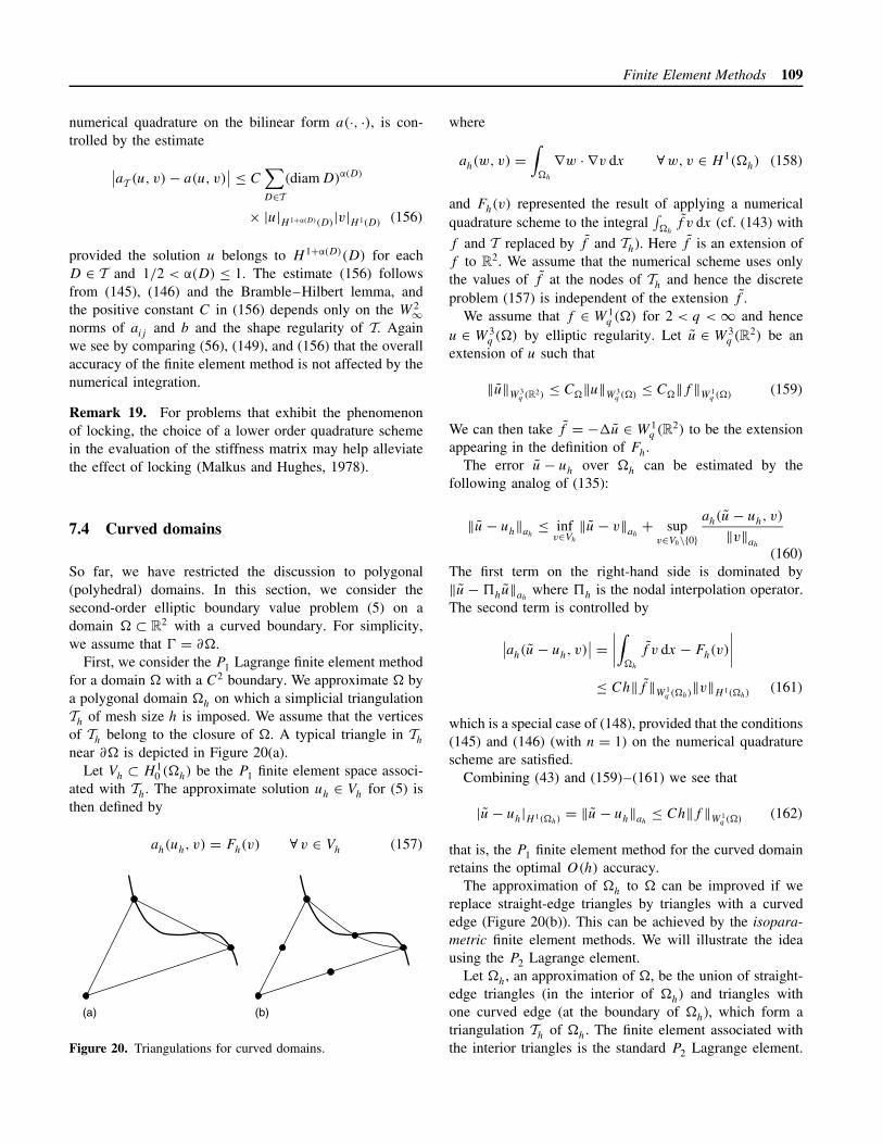
Finite Element Methods 109
numerical quadrature on the bilinear form a(·, ·), is con-trolled by the estimate∣∣aT (u, v)− a(u, v)
∣∣ ≤ C∑D∈T
(diam D)α(D)
× |u|H 1+α(D)(D)|v|H 1(D) (156)
provided the solution u belongs to H 1+α(D)(D) for eachD ∈ T and 1/2 < α(D) ≤ 1. The estimate (156) followsfrom (145), (146) and the Bramble–Hilbert lemma, andthe positive constant C in (156) depends only on the W 2∞norms of aij and b and the shape regularity of T. Againwe see by comparing (56), (149), and (156) that the overallaccuracy of the finite element method is not affected by thenumerical integration.
Remark 19. For problems that exhibit the phenomenonof locking, the choice of a lower order quadrature schemein the evaluation of the stiffness matrix may help alleviatethe effect of locking (Malkus and Hughes, 1978).
7.4 Curved domains
So far, we have restricted the discussion to polygonal(polyhedral) domains. In this section, we consider thesecond-order elliptic boundary value problem (5) on adomain � ⊂ R
2 with a curved boundary. For simplicity,we assume that � = ∂�.
First, we consider the P1 Lagrange finite element methodfor a domain � with a C2 boundary. We approximate � bya polygonal domain �h on which a simplicial triangulationTh of mesh size h is imposed. We assume that the verticesof Th belong to the closure of �. A typical triangle in Th
near ∂� is depicted in Figure 20(a).Let Vh ⊂ H 1
0 (�h) be the P1 finite element space associ-ated with Th. The approximate solution uh ∈ Vh for (5) isthen defined by
ah(uh, v) = Fh(v) ∀ v ∈ Vh (157)
(a) (b)
Figure 20. Triangulations for curved domains.
where
ah(w, v) =∫
�h
∇w · ∇v dx ∀w, v ∈ H 1(�h) (158)
and Fh(v) represented the result of applying a numericalquadrature scheme to the integral
∫�h
f v dx (cf. (143) with
f and T replaced by f and Th). Here f is an extension off to R
2. We assume that the numerical scheme uses onlythe values of f at the nodes of Th and hence the discreteproblem (157) is independent of the extension f .
We assume that f ∈ W 1q (�) for 2 < q < ∞ and hence
u ∈ W 3q (�) by elliptic regularity. Let u ∈ W 3
q (R2) be anextension of u such that
‖u‖W 3q (R2) ≤ C�‖u‖W 3
q (�) ≤ C�‖f ‖W 1q (�) (159)
We can then take f = −�u ∈ W 1q (R2) to be the extension
appearing in the definition of Fh.The error u− uh over �h can be estimated by the
following analog of (135):
‖u− uh‖ah≤ inf
v∈Vh
‖u− v‖ah+ sup
v∈Vh\{0}ah(u− uh, v)
‖v‖ah
(160)
The first term on the right-hand side is dominated by‖u−�hu‖ah
where �h is the nodal interpolation operator.The second term is controlled by
∣∣ah(u− uh, v)∣∣ = ∣∣∣∣∫
�h
f v dx − Fh(v)
∣∣∣∣≤ Ch‖f ‖W 1
q (�h)‖v‖H 1(�h)
(161)
which is a special case of (148), provided that the conditions(145) and (146) (with n = 1) on the numerical quadraturescheme are satisfied.
Combining (43) and (159)–(161) we see that
|u− uh|H 1(�h)= ‖u− uh‖ah
≤ Ch‖f ‖W 1q (�) (162)
that is, the P1 finite element method for the curved domainretains the optimal O(h) accuracy.
The approximation of �h to � can be improved if wereplace straight-edge triangles by triangles with a curvededge (Figure 20(b)). This can be achieved by the isopara-metric finite element methods. We will illustrate the ideausing the P2 Lagrange element.
Let �h, an approximation of �, be the union of straight-edge triangles (in the interior of �h) and triangles withone curved edge (at the boundary of �h), which form atriangulation Th of �h. The finite element associated withthe interior triangles is the standard P2 Lagrange element.
110 Finite Element Methods
For a triangle D at the boundary, we assume that there isa homeomorphism �D from the standard simplex S ontoD such that �D(x) = (�D,1(x), �D,2(x)) where �D,1(x)
and �D,2(x) are quadratic polynomials in x = (x1, x2). Thespace of shape functions P
Dis then defined by
PD= {v ∈ C∞(D) : v ◦�D ∈ P2(S)} (163)
that is, the functions in PD
are quadratic polynomials in thecurvilinear coordinates on D induced by �−1
D . The set ND
of nodal variables consist of pointwise evaluations of theshape functions at the nodes corresponding to the nodes ofthe P2 element on S (cf. Figures 2 and 20) under the map�D . We assume that all such nodes belong to � and thenodes on the curved edge of D belong to ∂� (cf. Figure 20).
In other words, the finite element (D,PD,N
D) is pulled
back to the P2 Lagrange finite element on S under �D .It is called an isoparametric element because the compo-nents of the parameterization map �D belong to the shapefunctions of the P2 element on S. The corresponding finiteelement space defined by (32) (with T replaced by Th) is asubspace of H 1(�h) that contains all the continuous piece-wise linear polynomials with respect to Th. By setting thenodal values on ∂�h to be zero, we have a finite elementspace Vh ⊂ H 1
0 (�h). The discrete problem for uh ∈ Vh isthen defined by
ah(uh, v) = Fh(v) (164)
where the numerical quadrature scheme in the definition ofFh involves only the nodes of the finite element space sothat the discrete problem is independent of the choice of theextension of f and the variational form ah(·, ·) is obtainedfrom ah(·, ·) by the numerical quadrature scheme.
We assume that f ∈ W 2q (�) for 1 < q < ∞ and hence
u ∈ W 4q (�) by elliptic regularity (assuming that � has a C3
boundary). Let u ∈ W 4q (R2) be an extension of u such that
‖u‖W 4q (R2) ≤ C�‖u‖W 4
q (�) ≤ C�‖f ‖W 2q (�) (165)
Under the condition (153), we have
ah(v, v) ≥ c|v|2H 1(�h)
∀ v ∈ Vh (166)
and the error of u− uh over �h can be estimated by thefollowing analog of (155)
|u− uh|H 1(�h)≤ inf
v∈Vh
|u− v|H 1(�h)
+ 1
c
{sup
v∈Vh\{0}ah(u, v)− ah(u, v)
|v|H 1(�h)
+ supv∈Vh\{0}
ah(u, v)− ah(uh, v)
|v|H 1(�h)
}(167)
The analysis of the terms on the right-hand side of (167)involves the shape regularity of a curved triangle, whichcan be defined as follows. Let AD be the affine map thatagrees with �D at the vertices of the standard simplex S,and D be the image of S under AD. (D is the triangle inFigure 20(a), while D is the curved triangle in (b).) Theshape regularity of the curved triangle D is measured bythe aspect ratio γ(D) (cf. (29)) of the straight-edged triangleD and the parameter κ(D) defined by
κ(D) = max{h−1|�D ◦A−1
D |W 1∞(D), h−2|�D ◦A−1
D |W 2∞(S)
}(168)
and we can take the aspect ratio γ(D) to be the maximumof γ(D) and κ(D). Note that in the case where D = D theparameter κ(D) = 0 and γ(D) = γ(D).
The first term on the right-hand side of (167) is domi-nated by ‖u−�hu‖ah
, where �h is the nodal interpolationoperator. Note that, by using the Bramble–Hilbert lemmaon S and scaling, we have the following generalizationof (43):
|u−�Du|H 1(D) ≤ C(diam D)2‖u‖H 3(D) (169)
where �D is the element nodal interpolation operator andthe constant C depends only on an upper bound of γ(D),and hence
‖u−�huh‖H 1(�h)≤ Ch2‖u‖H 3(�h)
(170)
In order to analyze the third term on the right-hand side of(167), we take f = −�u and impose the conditions (145)and (146) (with n = 2) on the numerical quadrature scheme.We then have the following special case of (148):
∣∣ah(u, v)− ah(uh, v)∣∣ = ∣∣∣∣∫
�h
f v dx − Fh(v)
∣∣∣∣≤ Ch2‖f ‖W 2
q (�h)|v|H 1(�h)
(171)
Similarly, the second term on the right-hand side of(167), which measures the effect of numerical integrationon the variational form ah(·, ·), is controlled by the estimate∣∣ah(u, v)− ah(u, v)
∣∣ ≤ Ch2|u|H 3(�h)|v|H 1(�h)
∀ v ∈ Vh
(172)
Combining (167) and (170)–(172) we have
‖u− uh‖ ≤ Ch2‖f ‖W 2q (�) (173)

Finite Element Methods 111
where C depends only on an upper bound of {γ(D) :D ∈ Th} and the constants in (165). Therefore, the P2isoparametric finite element method retains the optimalO(h2) accuracy. On the other hand, if only straight-edgedtriangles are used in the construction of �h, then theaccuracy of the P2 Lagrange finite element method is onlyof order O(h3/2) (Strang and Berger, 1971).
The discussion above can be generalized to higher-orderisoparametric finite element methods, higher dimensions,and elliptic problems with variable coefficients (Ciarlet,1978).
Remark 20. Estimates such as (160) and (162) are usefulonly when a sequence of domains �hi
with correspondingtriangulations Thi
can be constructed so that hi ↓ 0 and theaspect ratios of all the triangles (straight or curved) in thetriangulations remain bounded. We refer the readers to Scott(1973) for 2-D constructions and to Lenoir (1986) for the3-D case.
Remark 21. Other finite element methods for curveddomains can be found in Zlamal (1973, 1974), Scott (1975),and Bernardi (1989).
Remark 22. Let �i be a sequence of convex polygonsapproaching the unit disc. The displacement of the simplysupported plate on �i with unit loading does not convergeto the displacement of the simply supported plate on the unitdisc (also with unit loading) as i →∞. This is known asBabuska’s plate paradox (Babuska and Pitkaranta, 1990). Itshows that numerical solutions obtained by approximatinga curved domain with polygonal domains, in general, do notconverge to the solution of a fourth-order problem definedon the curved domain. We refer the readers to Mansfield(1978) for the construction of finite element spaces that aresubspaces of H 2(�).
7.5 Pointwise estimates
Besides the estimates in L2-based Sobolev spaces dis-cussed in Section 4, there also exist a priori error esti-mates for finite element methods in Lp-based Sobolevspaces with p = 2. In particular, error estimates in the L∞-based Sobolev spaces can provide pointwise error estimates.Below we describe some results for second-order ellip-tic boundary value problems with homogeneous Dirichletboundary conditions.
In the one-dimensional case (Wheeler, 1973) where �
is an interval, the finite element solution uT for a given
triangulation T with mesh size hT satisfies
‖u− uT ‖L∞(�) ≤ ChnT|u|Wn∞(�) (174)
provided the solution u of (5) belongs to Wn∞(�) and thefinite element space contains all the piecewise polynomialfunctions of degree ≤ n− 1. The estimate (174) also holdsin higher dimensions (Douglas, Dupont and Wheeler, 1974)in the case where � is a product of intervals and uT is thesolution in the Qn−1 finite element space of Example 7.
For a two-dimensional convex polygonal domain (Nat-terer, 1975; Scott, 1976, Nitsche, 1977), the estimate (174)holds in the case where n ≥ 3 and uT is the Pn−1 triangularfinite element solution for a general triangulation T. In thecase where uT is the P1 finite element solution, (174) isreplaced by
‖u− uT ‖L∞(�) ≤ Ch2T| ln hT | |u|W 2∞(�) (175)
L∞ estimates for general triangulations on polygonaldomains with reentrant corners and higher-dimensionaldomains can be found in Schatz and Wahlbin (1978,1979, 1982) and Schatz (1998). The estimate (175)was also established in Gastaldi and Nochetto (1987)for the Crouzeix-Raviart nonconforming P1 element ofExample 16.
It is also known (Rannacher and Scott, 1982; Brennerand Scott, 2002) that
|u− uT |W 1∞(�) ≤ C infv∈VT
C|u− v|W 1∞(�) (176)
where � is a convex polygonal domain in R2 and uT is
the Pn (n ≥ 1) triangular finite element solution obtainedfrom a general triangulation T of �. Optimal order estimatesfor |u− uT |W 1∞(�) can be derived immediately from (176).Extension of (176) to higher dimensions can be found inSchatz and Wahlbin (1995).
7.6 Interior estimates and pollution effects
Let � be the L-shaped polygon in Figure 1. The solutionu of the Poisson problem (5) on � with homogeneousDirichlet boundary condition is singular near the reentrantcorner and u ∈ H 2(�). Consequently, the error estimate|u− uT |H 1(�) ≤ ChT ‖f ‖L2(�) does not hold for the P1triangular finite element solution uT associated with a quasi-uniform triangulation T of mesh size hT.
However, u does belong to H 2(�δ) where �δ is thesubset of the points of � whose distances to the reentrant

112 Finite Element Methods
corner are strictly greater than the positive number δ.Therefore, it is possible that
|u− uT |H 1(�δ)≤ ChT ‖f ‖L2(�) (177)
That the estimate (177) indeed holds is a consequence ofthe following interior estimate (Nitsche and Schatz, 1974):
|u−uT |H 1(�δ)≤ C
(infv∈VT
|u− v|H 1(�δ/2)+ ‖u− uT ‖L2(�δ/2)
)(178)
where VT ⊂ H 10 (�) is the P1 triangular finite element
space. Interior estimates in various Sobolev norms can beestablished for subdomains of general � in R
d and generalfinite elements. We refer the readers to Wahlbin (1991) for asurvey of such results and to Schatz (2000) for some recentdevelopments.
On the other hand, since uT is obtained by solvinga global system that involves the nodal values near thereentrant corner of the L-shaped domain, the effect of thesingularity at the reentrant corner can propagate into otherparts of �. This is known as the pollution effect and isreflected, for example, by the following estimate (Wahlbin,
1984):
‖u− uT ‖L2(�) ≥ Ch2β
T (179)
where β = π/(3π/2) = 2/3. Similar estimates can also beestablished for other Sobolev norms.
7.7 Superconvergence
Let uT be the finite element solution of a second-orderelliptic boundary value problem. Suppose that the spaceof shape functions on each element contains all the polyno-mials of degree ≤ n but not all the polynomials of degreen+ 1. Then the L∞ norm of the error u− uT is at most oforder hn+1, even if the solution u is smooth. However, theabsolute value of u− uT at certain points can be of orderhn+1+σ for some σ > 0. This is known as the phenomenonof superconvergence and such points are the superconver-gence points for uT . Similarly, a point where the absolutevalue of a derivative of u− uT is of order hn+σ is a super-convergence point for the derivative of uT .
The division points of a partition T for a two pointboundary value problem with smooth coefficients provides
6
17
18
21
12
34
56
7
8
9
10
11
12
13
14
15
16
17
18
19
20
21
22
23
24
1312 11 10
9
8
7
14
15
16
1
5
4
32
19 20
(a)
−1.0 −1.0−0.5 −1.0
0 −1.00 −0.5
000.5 0
01.01.0 0.51.0 1.00.5 1.0
0 1.0−0.5 1.0−1.0 1.0−1.0 0.5−1.0 0−1.0 −0.5−0.5 −0.5−0.5 0−0.5 0.5
0 0.50.5 0.5
Coordinates
(b)
216
3171715
4181915201812141119
620
7212111
810
162
173
151718
4151918201412191120
621
7112110
8
117
24
161817
51814
51919132012
521
68
201021
9
Elements
(c)
Figure 21. Picture of a triangulation T=conv{(−1/2,−1), (−1,−1/2), (−1,−1)}, conv{(−1,−1/2), (−1/2,−1), (−1/2,−1/2)}, . . . ,conv{(1/2, 1), (1, 1/2), (1, 1)} with m = 24 triangles and n = 21 nodes (a). The picture indicates an enumeration of nodes (numbersin circles) and elements (numbers in boxes) given in the matrices coordinates (b) and elements (c). The Dirichlet boundaryconditions on the exterior nodes are included in the vector dirichlet = (1, 2, 3, 4, 5, 6, 7, 8, 9, 10, 11, 12, 13, 14, 15, 16) of thelabels in a counterclockwise enumeration. The data coordinates, elements, and dirichlet are the input of the finite elementprogram to compute a displacement vector x as its output.
Finite Element Methods 113
the simplest example of superconvergence points. Let uTbe the finite element solution from the Pn Lagrange finiteelement space. Since the Green’s function Gp associatedwith a division point p is continuous in the interval �
and smooth on the two subintervals divided by p, we have(Douglas and Dupont, 1974)
|(u− uT )(p)| = |a(u− uT ,Gp)|= |a(u− uT , Gp −�N
T Gp)|≤ C‖u− uT ‖H 1(�)‖Gp −�N
T Gp)‖H 1(�) ≤ Ch2n
provided that u is sufficiently smooth. Therefore, p is asuperconvergence point for uT if n ≥ 2.
For general superconvergence results in variousdimensions, we refer the readers to Krızek andNeittaanmaki (1987), Chen and Huang (1995), Wahlbin(1995), Lin and Yan (1996), Schatz, Sloan and Wahlbin(1996), Krızek, Neittaanmaki and Stenberg (1998), Chen(1999), and Babuska and Strouboulis (2001).
7.8 Finite element program in 15 lines ofMATLAB
It is the purpose of this section to introduce a short (two-dimensional) P1 finite element program.
The data for a given triangulation T = {T1, . . . , Tm}into triangles with a set of nodes N = {z1, . . . , zn} aredescribed in user-specified matrices called coordinates
and elements. Figure 21 displays a triangulation withm triangles and n nodes as well as a fixed enumerationand the corresponding data. The coordinates of the nodeszk = (xk, yk) (d real components in general) are stored inthe kth row of the two-dimensional matrix coordinates.Each element Tj = conv{zk, z�, zm} is represented bythe labels of its vertices (k, �,m) stored in the j throw of the two-dimensional matrix elements. Thechosen permutation of (k, �, m) describes the elementin a counterclockwise orientation. Homogeneous Dirichletconditions are prescribed on the boundary specified by aninput vector dirichlet of all fixed nodes at the outerboundary; cf. Figure 21.
Given the aforementioned data in the model Dirichletproblem with right-hand side f = 1, the P1 finite ele-ment space V := span{ϕj : zj ∈ K} is formed by the nodalbasis functions ϕj of each free node zk; the set K offree nodes, the interior nodes, is represented in the N
vector freenodes, the vector of labels in 1 : n withoutdirichlet.
The resulting discrete equation is the N ×N linearsystem of equations Ax = b with the positive definite
symmetric stiffness matrix A and right-hand side b. Theircomponents are defined (as a subset of)
Ajk :=∫
�
∇ϕj · ∇ϕk dx
and
bj :=∫
�
f ϕj dx for j, k = 1, . . . , n
The computation of the entries Ajk and bj is performedelementwise for the additivity of the integral and since T isa partition of the domain �. Given the triangle Tj num-ber j , the MATLAB command coordinates(ele-
ments(j,:),:) returns the 3× 2 matrix (P1, P2, P3)T of
its vertices. Then, the local stiffness matrix reads
STIMA(Tj )αβ :=∫
Tj
∇ϕk · ∇ϕ� dx for α, β = 1, 2, 3
for those numbers k and � of two vertices zk = Pα and z� =Pβ of Tj . The correspondence of global and local indices,i.e. the numbers of vertices in (zk, z�, zm) = (P1, P2, P3),of Tj can be formalized by
I (Tj ) = {(α, k) ∈ {1, 2, 3} × {1, . . . , n} : Pα = zk ∈ N}
The local stiffness matrix is in fact
STIMA(Tj ) = detP
2(QQT ) with P :=
[1 1 1P1 P2 P3
]
and Q := P−1
0 01 00 1
This formula allows a compact programming in MATLABas shown (for any dimension d)
function stima=stima(vertices)P=[ones(1,size(vertices,2)+1);vertices’];Q=P\[zeros(1,size(vertices,2));. . .
eye(size(vertices,2))];stima=det(P)∗Q∗Q’/prod(1:size(vertices,2));
Utilizing the index sets I , the assembling of all localstiffness matrices reads
STIMA =∑Tj∈T
∑(α,k)∈I (Tj )
∑(β,�)∈I (Tj )
STIMA(Tj )αβ ek ⊗ e�
(ek is the kth canonical unit vector with the �th componentequal to the Kronecker delta δk� and ⊗ is the dyadicproduct.) The implementation of each summation is realizedby adding STIMA(Tj ) to the 3× 3 submatrix of the rowsand columns corresponding to k, �, m; see the MATLABprogram below.
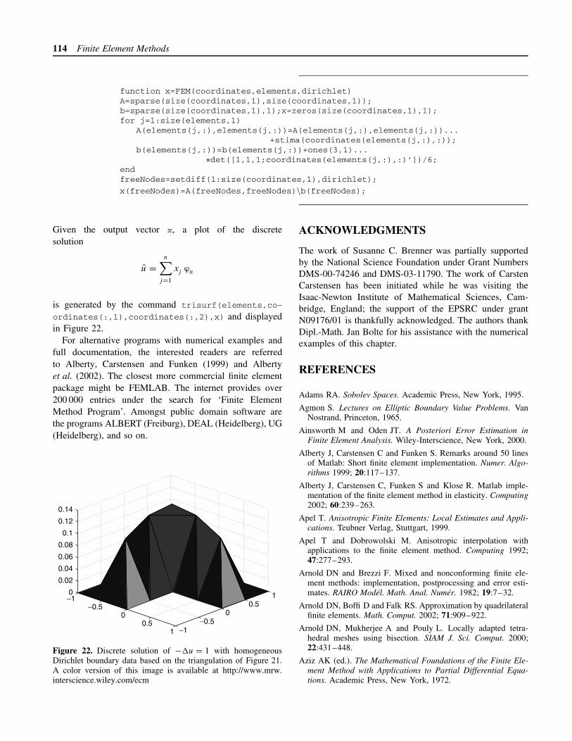
114 Finite Element Methods
function x=FEM(coordinates,elements,dirichlet)A=sparse(size(coordinates,1),size(coordinates,1));b=sparse(size(coordinates,1),1);x=zeros(size(coordinates,1),1);for j=1:size(elements,1)
A(elements(j,:),elements(j,:))=A(elements(j,:),elements(j,:))...+stima(coordinates(elements(j,:),:));
b(elements(j,:))=b(elements(j,:))+ones(3,1)...∗det([1,1,1;coordinates(elements(j,:),:)’])/6;
endfreeNodes=setdiff(1:size(coordinates,1),dirichlet);
x(freeNodes)=A(freeNodes,freeNodes)\b(freeNodes);
Given the output vector x, a plot of the discretesolution
u =n∑
j=1
xj ϕn
is generated by the command trisurf(elements,co-
ordinates(:,1),coordinates(:,2),x) and displayedin Figure 22.
For alternative programs with numerical examples andfull documentation, the interested readers are referredto Alberty, Carstensen and Funken (1999) and Albertyet al. (2002). The closest more commercial finite elementpackage might be FEMLAB. The internet provides over200 000 entries under the search for ‘Finite ElementMethod Program’. Amongst public domain software arethe programs ALBERT (Freiburg), DEAL (Heidelberg), UG(Heidelberg), and so on.
−1−0.5
00.5
1 −1−0.5
00.5
10
0.02
0.04
0.06
0.08
0.1
0.12
0.14
Figure 22. Discrete solution of −�u = 1 with homogeneousDirichlet boundary data based on the triangulation of Figure 21.A color version of this image is available at http://www.mrw.interscience.wiley.com/ecm
ACKNOWLEDGMENTS
The work of Susanne C. Brenner was partially supportedby the National Science Foundation under Grant NumbersDMS-00-74246 and DMS-03-11790. The work of CarstenCarstensen has been initiated while he was visiting theIsaac-Newton Institute of Mathematical Sciences, Cam-bridge, England; the support of the EPSRC under grantN09176/01 is thankfully acknowledged. The authors thankDipl.-Math. Jan Bolte for his assistance with the numericalexamples of this chapter.
REFERENCES
Adams RA. Sobolev Spaces. Academic Press, New York, 1995.
Agmon S. Lectures on Elliptic Boundary Value Problems. VanNostrand, Princeton, 1965.
Ainsworth M and Oden JT. A Posteriori Error Estimation inFinite Element Analysis. Wiley-Interscience, New York, 2000.
Alberty J, Carstensen C and Funken S. Remarks around 50 linesof Matlab: Short finite element implementation. Numer. Algo-rithms 1999; 20:117–137.
Alberty J, Carstensen C, Funken S and Klose R. Matlab imple-mentation of the finite element method in elasticity. Computing2002; 60:239–263.
Apel T. Anisotropic Finite Elements: Local Estimates and Appli-cations. Teubner Verlag, Stuttgart, 1999.
Apel T and Dobrowolski M. Anisotropic interpolation withapplications to the finite element method. Computing 1992;47:277–293.
Arnold DN and Brezzi F. Mixed and nonconforming finite ele-ment methods: implementation, postprocessing and error esti-mates. RAIRO Model. Math. Anal. Numer. 1982; 19:7–32.
Arnold DN, Boffi D and Falk RS. Approximation by quadrilateralfinite elements. Math. Comput. 2002; 71:909–922.
Arnold DN, Mukherjee A and Pouly L. Locally adapted tetra-hedral meshes using bisection. SIAM J. Sci. Comput. 2000;22:431–448.
Aziz AK (ed.). The Mathematical Foundations of the Finite Ele-ment Method with Applications to Partial Differential Equa-tions. Academic Press, New York, 1972.

Finite Element Methods 115
Babuska I. Courant element: before and after. Lecture Notes inPure and Applied Mathematics, vol. 164. Marcel Dekker: NewYork, 1994; 37–51.
Babuska I and Aziz AK. Survey lectures on the mathematicalfoundations of the finite element method. In The MathematicalFoundations of the Finite Element Method with Applications toPartial Differential Equations, Aziz AK (ed.). Academic Press,New York, 1972; 3–359.
Babuska I and Aziz AK. On the angle condition in the finiteelement method. SIAM J. Numer. Anal. 1976; 13:214–226.
Babuska I and Guo B. The h, p, and h− p versions of thefinite element methods in 1 dimension. Numer. Math. 1986;49:613–657.
Babuska I and Kellogg RB. Nonuniform error estimates for the fi-nite element method. SIAM J. Numer. Anal. 1975; 12:868–875.
Babuska I and Miller A. A feedback finite element method witha posteriori error estimation. I. The finite element method andsome properties of the a posteriori estimator. Comput. MethodsAppl. Mech. Eng. 1987; 61:1–40.
Babuska I and Osborn J. Eigenvalue problems. In Handbook ofNumerical Analysis, vol. II, Ciarlet PG and Lions JL (eds).North Holland: Amsterdam, 1991; 641–787.
Babuska I and Pitkaranta J. The plate paradox for hard and softsimple support. SIAM J. Math. Anal. 1990; 21:551–576.
Babuska I and Rheinboldt WC. Error estimates for adaptivefinite element computations. SIAM J. Numer. Anal. 1978;15:736–754.
Babuska I and Rheinboldt WC. Analysis of optimal finite-elementmeshes in R
1. Math. Comput. 1979; 33:435–463.
Babuska I and Strouboulis T. The Finite Element Method and itsReliability. Oxford University Press, New York, 2001.
Babuska I and Suri M. On locking and robustness in the finiteelement method. SIAM J. Numer. Anal. 1992; 29:1261–1293.
Babuska I and Vogelius R. Feedback and adaptive finite elementsolution of one-dimensional boundary value problems. Numer.Math. 1984; 44:75–102.
Bangerth W and Rannacher R. Adaptive Finite Element Meth-ods for Differential Equations, Lectures in Mathematics ETHZurich. Birkhauser Verlag, Basel, 2003.
Bank RE and Weiser A. Some a posteriori error estimators for ell-iptic differential equations. Math. Comput. 1985; 44:283–301.
Bank RE and Xu J. Asymptotically Exact a Posteriori Error Esti-mators, Part I: Grids with Superconvergence. SIAM J. Numer.Anal. 2003; 41:2294–2312.
Bansch E. Local mesh refinement in 2 and 3 dimensions. IMPACTComput. Sci. Eng. 1991; 3:181–191.
Bartels S and Carstensen C. Each averaging technique yieldsreliable a posteriori error control in FEM on unstructured grids.II. Higher order FEM. Math. Comput. 2002; 71:971–994.
Bathe K-J. Finite Element Procedures. Prentice Hall, Upper Sad-dle River, 1996.
Becker EB, Carey GF and Oden JT. Finite Elements. An Intro-duction. Prentice Hall, Englewood Cliffs, 1981.
Becker R and Rannacher R. A feed-back approach to error controlin finite element methods: basic analysis and examples. East-West J. Numer. Math. 1996; 4:237–264.
Becker R and Rannacher R. An optimal control approach to aposteriori error estimation in finite element methods. ActaNumer. 2001; 10:1–102.
Ben Belgacem F and Brenner SC. Some nonstandard finite ele-ment estimates with applications to 3D Poisson and Signoriniproblems. Electron. Trans. Numer. Anal. 2001; 12:134–148.
Berger A, Scott R and Strang G. Approximate boundary condi-tions in the finite element method. Symposia Mathematica,vol. X (Convegno di Analisi Numerica, INDAM, Rome, 1972).Academic Press: London, 1972; 295–313.
Bernardi C. Optimal finite-element interpolation on curved do-mains. SIAM J. Numer. Anal. 1989; 26:1212–1240.
Bernardi C and Girault V. A local regularization operator fortriangular and quadrilateral finite elements. SIAM J. Numer.Anal. 1998; 35:1893–1916.
Bey J. Tetragonal grid refinement. Computing 1995; 55:355–378.
Binev P, Dahmen W and DeVore R. Adaptive finite elementmethods with convergence rates. Numer. Math. 2004; 97:219–268.
Braess D. Finite Elements (2nd edn). Cambridge University Press,Cambridge, 2001.
Bramble JH and Hilbert AH. Estimation of linear functionals onSobolev spaces with applications to Fourier transforms andspline interpolation. SIAM J. Numer. Anal. 1970; 7:113–124.
Bramble JH, Pasciak JE and Schatz AH. The construction ofpreconditioners for elliptic problems by substructuring, I. Math.Comput. 1986; 47:103–134.
Bramble JH, Pasciak JE and Steinbach O. On the stability of theL2-projection in H 1(�). Math. Comput. 2002; 71:147–156.
Brenner SC and Scott LR. The Mathematical Theory of FiniteElement Methods (2nd edn). Springer-Verlag, New York, 2002.
Brenner SC and Sung LY. Discrete Sobolev and Poincare inequal-ities via Fourier series. East-West J. Numer. Math. 2000;8:83–92.
Carstensen C. Quasi-interpolation and a posteriori error analysisin finite element methods. M2AN Math. Model. Numer. Anal.1999; 33:1187–1202.
Carstensen C. Merging the Bramble-Pasciak-Steinbach and theCrouzeix-Thomee criterion for H 1-stability of the L2-projectiononto finite element spaces. Math. Comput. 2002; 71:157–163.
Carstensen C. All first-order averaging techniques for a posteriorifinite element error control on unstructured grids are efficientand reliable. Math. Comput. 2004; 73:1153–1165.
Carstensen C. An adaptive mesh-refining algorithm allowingfor an H 1-stable L2-projection onto Courant finite elementspaces. Constructive Approximation Theory. Newton Institute,2003b; DOI: 10.1007/s00365-003-0550-5. Preprint NI03004-CPD available at http://www.newton.cam.ac.uk/preprints/NI03004.pdf.
Carstensen C. Some remarks on the history and future of aver-aging techniques in a posteriori finite element error analysis.ZAMM 2004; 84:3–21.
Carstensen C and Alberty J. Averaging techniques for reliable aposteriori FE-error control in elastoplasticity with hardening.Comput. Methods Appl. Mech. Eng. 2003; 192:1435–1450.
116 Finite Element Methods
Carstensen C and Bartels S. Each averaging technique yieldsreliable a posteriori error control in FEM on unstructured grids.I. Low order conforming, nonconforming and Mixed FEM.Math. Comput. 2002; 71:945–969.
Carstensen C and Funken SA. Fully reliable localised error con-trol in the FEM. SIAM J. Sci. Comput. 1999/00; 21:1465–1484.
Carstensen C and Funken SA. Constants in Clement-interpolationerror and residual based a posteriori estimates in finite elementmethods. East-West J. Numer. Math. 2000; 8:153–175.
Carstensen C and Funken SA. A posteriori error control in low-order finite element discretizations of incompressible stationaryflow problems. Math. Comput. 2001a; 70:1353–1381.
Carstensen C and Funken SA. Averaging technique for FE-a pos-teriori error control in elasticity. I: Conforming FEM. II: λ-independent estimates. III: Locking-free nonconforming FEM.Comput. Methods Appl. Mech. Eng. 2001b; 190:2483–2498;190:4663–4675; 191:861–877.
Carstensen C and Verfurth R. Edge residuals dominate a posteriorierror estimates for low order finite element methods. SIAM J.Numer. Anal. 1999; 36:1571–1587.
Carstensen C, Bartels S and Klose R. An experimental survey ofa posteriori Courant finite element error control for the Poissonequation. Adv. Comput. Math. 2001; 15:79–106.
Chen C. Superconvergence for triangular finite elements. Sci.China (Ser. A) 1999; 42:917–924.
Chen CM and Huang YQ. High Accuracy Theory of FiniteElement Methods. Hunan Scientific and Technical Publisher,Changsha, 1995 (in Chinese).
Ciarlet PG. The Finite Element Method for Elliptic Problems.North Holland, Amsterdam, 1978 (Reprinted in the Classicsin Applied Mathematics Series, SIAM, Philadelphia, 2002).
Ciarlet PG. Mathematical Elasticity, Volume I: Three-dimensionalElasticity. North Holland, Amsterdam, 1988.
Ciarlet PG. Basic error estimates for elliptic problems. In Hand-book of Numerical Analysis, vol. II, Ciarlet PG and Lions JL(eds). North Holland: Amsterdam, 1991; 17–351.
Ciarlet PG. Mathematical Elasticity, Volume II: Theory of Plates.North Holland, Amsterdam, 1997.
Clement P. Approximation by finite element functions usinglocal regularization. RAIRO Model. Math. Anal. Numer. 1975;9:77–84.
Courant R. Variational methods for the solution of problems ofequilibrium and vibration. Bull. Am. Math. Soc. 1943; 49:1–23.
Crouzeix M and Raviart PA. Conforming and nonconformingfinite element methods for solving the stationary Stokes equa-tions I. RAIRO Model. Math. Anal. Numer. 1973; 7:33–75.
Crouzeix M and Thomee V. The stability in Lp and W 1,p of theL2-projection onto finite element function paces. Math. Comput.1987; 48:521–532.
Dauge M. Elliptic Boundary Value Problems on Corner Domains.Lecture Notes in Mathematics 1341. Springer-Verlag, Berlin,1988.
Davis PJ and Rabinowitz P. Methods of Numerical Integration.Academic Press, Orlando, 1984.
Demkowicz, L. hp-adaptive finite elements for time-harmonicMaxwell equations. Topics in Computational Wave Propaga-tion, Lecture Notes in Computational Science and Engineering,
pp. 163–199, Ainsworth M, Davies P, Duncan D, Martin P andRynne B (eds). Springer-Verlag, Berlin, 2003.
Dorfler W. A convergent adaptive algorithm for Poison’s equa-tion. SIAM J. Numer. Anal. 1996; 33:1106–1124.
Dorfler W and Nochetto RH. Small data oscillation implies thesaturation assumption. Numer. Math. 2002; 91:1–12.
Douglas Jr J and Dupont T. Galerkin approximations for thetwo-point boundary value problem using continuous, piecewisepolynomial spaces. Numer. Math. 1974; 22:99–109.
Douglas Jr J, Dupont T and Wheeler MF. An L∞ estimate anda superconvergence result for a Galerkin method for ellipticequations based on tensor products of piecewise polynomials.RAIRO Model. Math. Anal. Numer. 1974; 8:61–66.
Douglas Jr J, Dupont T, Percell P and Scott R. A family ofC1 finite elements with optimal approximation properties forvarious Galerkin methods for 2nd and 4th order problems.RAIRO Model. Math. Anal. Numer. 1979; 13:227–255.
Dupont T and Scott R. Polynomial approximation of functions inSobolev spaces. Math. Comput. 1980; 34:441–463.
Duvaut G and Lions JL. Inequalities in Mechanics and Physics.Springer-Verlag, Berlin, 1976.
Eriksson K and Johnson C. Adaptive finite element methods forparabolic problems. I. A linear model problem. SIAM J. Numer.Anal. 1991; 28:43–77.
Eriksson K, Estep D, Hansbo P and Johnson C. Introduction toadaptive methods for differential equations. Acta Numer. 1995;4:105–158.
Friedrichs KO. On the boundary value problems of the theory ofelasticity and Korn’s inequality. Ann. Math. 1947; 48:441–471.
Gastaldi L and Nochetto RH. Optimal L∞-error estimates fornonconforming and mixed finite element methods of lowestorder. Numer. Math. 1987; 50:587–611.
Gilbarg D and Trudinger NS. Elliptic Partial Differential Equa-tions of Second Order (2nd edn). Springer-Verlag, Berlin, 1983.
Girault V and Scott LR. Hermite interpolation of nonsmoothfunctions preserving boundary conditions. Math. Comput. 2002;71:1043–1074.
Grisvard P. Elliptic Problems in Nonsmooth Domains. Pitman,Boston, 1985.
Hughes TJR. The Finite Element Method. Linear Static andDynamic Finite Element Analysis. Prentice Hall, EnglewoodCliffs, 1987 (Reprinted by Dover Publications, New York,2000).
Jamet P. Estimations d’erreur pour des elements finis droitspresque degeneres. RAIRO Anal. Numer. 1976; 10:43–61.
Kozlov VA, Maz’ya VG and Rossman J. Elliptic Boundary ValueProblems in Domains with Point Singularities. American Math-ematical Society, 1997.
Kozlov VA, Maz’ya VG and Rossman J. Spectral Problems Asso-ciated with Corner Singularities of Solutions to Elliptic Prob-lems. American Mathematical Society, 2001.
Krızek M and Neittaanmaki P. On superconvergence techniques.Acta Appl. Math. 1987; 9:175–198.
Krızek M, Neittaanmaki P and Stenberg R (eds.). Finite ElementMethods: Superconvergence, Post-processing and A Posteriori
Finite Element Methods 117
Estimates, Proc. Conf. Univ. of Jyvaskyla, 1996, Lecture Notesin Pure and Applied Mathematics 196. Marcel Dekker, NewYork, 1998.
Ladeveze P and Leguillon D. Error estimate procedure in thefinite element method and applications. SIAM J. Numer. Anal.1983; 20:485–509.
Lenoir M. Optimal isoparametric finite elements and error esti-mates for domains involving curved boundaries. SIAM J.Numer. Anal. 1986; 23:562–580.
Lin Q and Yan NN. Construction and Analysis of Efficient FiniteElement Methods. Hebei University Press, Baoding, 1996 (inChinese).
Mansfield L. Approximation of the boundary in the finite elementsolution of fourth order problems. SIAM J. Numer. Anal. 1978;15:568–579.
Malkus DS and Hughes TJR. Mixed finite element methods-reduced and selective integration techniques: A unification ofconcepts. Comput. Methods Appl. Mech. Eng. 1978; 15:63–81.
Morin P, Nochetto RH and Siebert KG. Local problems on stars:a posteriori error estimation, convergence, and performance.Math. Comput. 2003a; 72:1067–1097.
Morin P, Nochetto RH and Siebert KG. Convergence of adaptivefinite element methods. SIAM Rev. 2003b; 44:631–658.
Natterer F. Uber die punktweise Konvergenz finiter Elemente.Numer. Math. 1975; 25:67–77.
Nazarov SA and Plamenevsky BA. Elliptic Problems in Domainswith Piecewise Smooth Boundaries. Walter De Gruyter, Berlin,1994.
Necas J. Les Methodes Directes en Theorie des Equations Ellip-tiques. Masson, Paris, 1967.
Nicaise S. Polygonal Interface Problems. Peter D Lang Verlag,Frankfurt am Main, 1993.
Nitsche JA. L∞-convergence of finite element approximations.In Mathematical Aspects of Finite Element Methods, LectureNotes in Mathematics 606. Springer-Verlag: New York, 1977;261–274.
Nitsche JA. On Korn’s second inequality. RAIRO Anal. Numer.1981; 15:237–248.
Nitsche JA and Schatz AH. Interior estimates for Ritz-Galerkinmethods. Math. Comput. 1974; 28:937–958.
Nochetto RH. Removing the saturation assumption in a posteriorierror analysis. Istit. Lombardo Accad. Sci. Lett. Rend. A 1993;127:67–82.
Nochetto RH and Wahlbin LB. Positivity preserving finite ele-ment approximation. Math. Comput. 2002; 71:1405–1419.
Oden JT. Finite elements: an introduction. In Handbook of Numer-ical Analysis, vol. II, Ciarlet PG and Lions JL (eds). NorthHolland: Amsterdam, 1991; 3–15.
Oden JT and Demkowicz LF. Applied Functional Analysis. CRCPress, Boca Raton, 1996.
Oden JT and Reddy JN. An Introduction to the MathematicalTheory of Finite Elements. Wiley, New York, 1976.
Rannacher R and Scott R. Some optimal error estimates for piece-wise linear finite element approximations. Math. Comput. 1982;38:437–445.
Reddy JN. Applied Functional Analysis and Variational Methodsin Engineering. McGraw-Hill, New York, 1986.
Rivara MC. Algorithms for refining triangular grids suitable foradaptive and multigrid techniques. Int. J. Numer. Methods Eng.1984; 20:745–756.
Rodriguez R. Some remarks on Zienkiewicz-Zhu estimator. Nu-mer. Methods Partial Diff. Equations 1994a; 10:625–635.
Rodriguez R. A posteriori error analysis in the finite elementmethod. In Lecture Notes in Pure and Applied Mathematics,vol. 164. Marcel Dekker: New York, 1994b; 389–397.
Schatz AH. An observation concerning Ritz-Galerkin meth-ods with indefinite bilinear forms. Math. Comput. 1974;28:959–962.
Schatz AH. Pointwise error estimates and asymptotic error expan-sion inequalities for the finite element method on irreg-ular grids: Part I. Global estimates. Math. Comput. 1998;67:877–899.
Schatz AH. Pointwise error estimates and asymptotic error expan-sion inequalities for the finite element method on irregulargrids: Part II. Interior estimates. SIAM J. Numer. Anal. 2000;38:1269–1293.
Schatz AH and Wahlbin LB. Maximum norm estimates in thefinite element method on plane polygonal domains. Part 1.Math. Comput. 1978; 32:73–109.
Schatz AH and Wahlbin LB. Maximum norm estimates in thefinite element method on plane polygonal domains. Part 2.Math. Comput. 1979; 33:465–492.
Schatz AH and Wahlbin LB. On the quasi-optimality in L∞ of the◦
H1-projection into finite element spaces. Math. Comput. 1982;
38:1–22.
Schatz AH and Wahlbin LB. Interior maximum-norm estimatesfor finite element methods, Part II. Math. Comput. 1995;64:907–928.
Schatz AH, Sloan IH and Wahlbin LB. Superconvergence in finiteelement methods and meshes that are locally symmetric withrespect to a point. SIAM J. Numer. Anal. 1996; 33:505–521.
Schatz AH, Thomee V and Wendland WL. Mathematical Theoryof Finite and Boundary Element Methods. Birkhauser Verlag,Basel, 1990.
Scott R. Finite Element Techniques for Curved Boundaries. Doc-toral thesis, Massachusetts Institute of Technology, 1973.
Scott R. Interpolated boundary conditions in the finite elementmethod. SIAM J. Numer. Anal. 1975; 12:404–427.
Scott R. Optimal L∞ estimates for the finite element method onirregular meshes. Math. Comput. 1976; 30:681–697.
Scott LR and Zhang S. Finite element interpolation of non-smoothfunctions satisfying boundary conditions. Math. Comput. 1990;54:483–493.
Strang G and Berger A. The change in solution due to change indomain. Proceedings AMS Symposium on Partial DifferentialEquations. American Mathematical Society: Providence, 1971;199–205.
Strang G. and Fix GJ. An Analysis of the Finite Element Method.Prentice Hall, Englewood Cliffs, 1973 (Reprinted by Wellesley-Cambridge Press, Wellesley, 1988).
118 Finite Element Methods
Szabo BA and Babuska I. Finite Element Analysis. John Wiley &Sons, New York, 1991.
Triebel H. Interpolation Theory, Function Spaces, DifferentialOperators. North Holland, Amsterdam, 1978.
Verfurth R. A Review of A Posteriori Error Estimation and Adap-tive Mesh-Refinement Techniques. Wiley-Teubner, New York,1996.
Verfurth R. A note on polynomial approximation in Sobolevspaces. Model. Math. Anal. Numer. 1999; 33:715–719.
Wahlbin LB. On the sharpness of certain local estimates for ◦H
1
projections into finite element spaces: Influence of a reentrantcorner. Math. Comput. 1984; 42:1–8.
Wahlbin LB. Local behavior in finite element methods. In Hand-book of Numerical Analysis, vol. II, Ciarlet PG, Lions JL (eds).North Holland: Amsterdam, 1991; 355–522.
Wahlbin LB. Superconvergence in Galerkin Finite Element Meth-ods, Lecture Notes in Mathematics 1605. Springer-Verlag,Berlin, 1995.
Wheeler MF. An optimal L∞ error estimate for Galerkin approx-imations to solutions of two-point boundary value problems.SIAM J. Numer. Anal. 1973; 1:914–917.
Wloka J. Partial Differential Equations. Cambridge UniversityPress, Cambridge, 1987.
Yosida K. Functional Analysis, Classics in Mathematics. Springer-Verlag, Berlin, 1995.
Zienkiewicz OC and Taylor RL. The Finite Element Method (5thedn). Butterworth-Heinemann, Oxford, 2000.
Zlamal M. Curved elements in the finite element method. I. SIAMJ. Numer. Anal. 1973; 10:229–240.
Zlamal M. Curved elements in the finite element method. II. SIAMJ. Numer. Anal. 1974; 11:347–362.
Zenisek A. Maximum-angle condition and triangular finite ele-ment of Hermite type. Math. Comput. 1995; 64:929–941.