chapter 22opt.zju.edu.cn/zjuopt2/upload/resources/chapter22 fiber-optic... · chapter 22...
TRANSCRIPT
CHAPTER
22 FIBER-OPTIC COMMUNICATIONS
22.1 COMPONENTS OF THE OPTICAL FIBER LINK A. Optical Fibers
B. Sources for Optical Transmitters
C. Detectors for Optical Receivers D. Fiber-Optic Systems
22.2 MODULATION, MULTIPLEXING, AND COUPLING
A. Modulation B. Multiplexing
C. Couplers
22.3 SYSTEM PERFORMANCE A. Digital Communication System B. Analog Communication System
22.4 RECEIVER SENSITIVITY
22.5 COHERENT OPTICAL COMMUNICATIONS A. Heterodyne Detection B. Performance of the Analog Heterodyne Receiver C. Performance of the Digital Heterodyne Receiver D. Coherent Systems
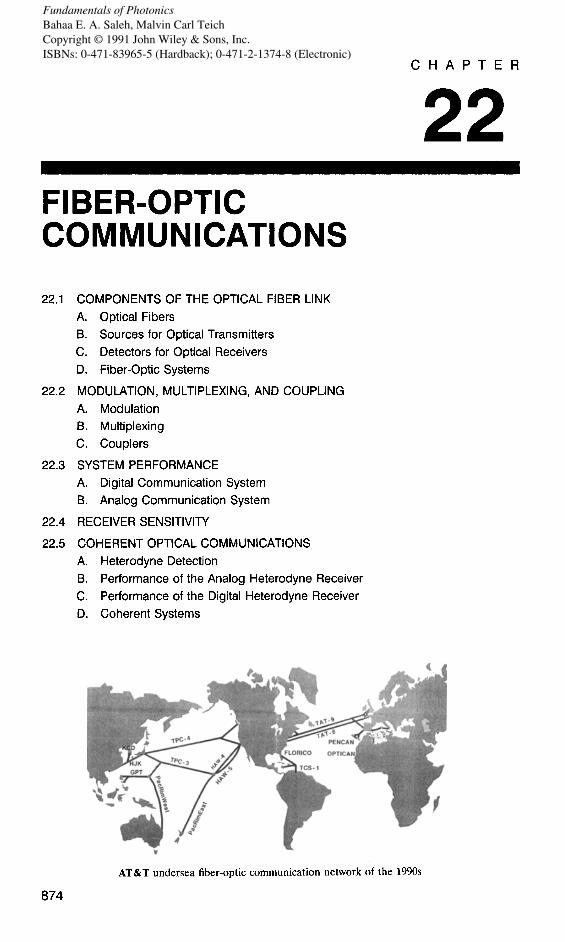
AT&T undersea fiber-optic communication network of the 1990s
874
Fundamentals of PhotonicsBahaa E. A. Saleh, Malvin Carl TeichCopyright © 1991 John Wiley & Sons, Inc.ISBNs: 0-471-83965-5 (Hardback); 0-471-2-1374-8 (Electronic)
Until recently, virtually all communication systems have relied on the transmission of information over electrical cables or have made use of radio-frequency and microwave electromagnetic radiation propagating in free space. It would appear that the use of light would have been a more natural choice for communications since, unlike electric- ity and radio waves, it did not have to be discovered. The reasons for the delay in the development of this technology are twofold: the difficulty of producing a light source that could be rapidly switched on and off and therefore could encode information at a high rate, and the fact that light is easily obstructed by opaque objects such as clouds, fog, smoke, and haze. Unlike radio-frequency and microwave radiation, light is rarely suitable for free-space communication.
Lightwave communications has recently come into its own, however, and indeed it is now the preferred technology in many applications. It is used for the transmission of voice, data, telemetry, and video in long-distance and local-area networks, and is suitable for a great diversity of other applications (e.g., cable television). Lightwave technology affords the user enormous transmission capacity, distant spacings of re- peaters, immunity from electromagnetic interference, and relative ease of installation.
The spectacular successes of fiber-optic communications have their roots in two critical photonic inventions: the development of the light-emitting diode (LED) and the development of the low-loss optical fiber as a light conduit. Suitable detectors of light have been available for some time, although their performance has been improved dramatically in recent years. Interest in optical communications was initially stirred by the invention of the laser in the early 1960s. However, the first generation of fiber-optic communication systems made use of LED sources and indeed many present local-area commercial systems continue to do so. Nevertheless, most lightwave communication systems (such as long-haul single-mode fiber-optic systems and short-haul free-space systems) do benefit from the large optical power, narrow linewidth, and high directivity provided by the laser. The proposed extension of the fiber network to reach individual dwellings will rely on the use of diode lasers.
A fiber-optic communication system comprises three basic elements: a compact light source, a low-loss/low-dispersion optical fiber, and a photodetector. These optical components have been discussed in Chaps. 16, 8, and 17, respectively. In this chapter we examine their role in the context of the overall design, operation, and performance of an optical communication link. Optical accessories such as connectors, couplers, switches, and multiplexing devices, as well as splices, are also essential to the successful operation of fiber links and networks. Optical-fiber amplifiers have also proved them- selves to be very valuable adjuncts to such systems. The principles of some of these devices have been discussed in Chap. 21 and in other parts of this book.
Although the waveguiding properties of different types of optical fibers have been discussed in detail in Chap. 8, this material is reviewed in Sec. 22.1 (in abbreviated form) to make this chapter self-contained. A brief summary of the properties of semiconductor photon sources and detectors suitable for fiber-optic communication systems is also provided in this section. This is followed, in Sec. 22.2, by an introduction to modulation, multiplexing, and coupling systems used in fiber-optic communications.
875
876 FIBER-OPTIC COMMUNICATIONS
Section 22.3 introduces the basic design principles applicable to long-distance digital and analog fiber-optic communication systems. The maximum fiber length that can be used to transmit data (at a given rate and with a prescribed level of performance) is determined. Performance deteriorates if the data rate exceeds the fiber bandwidth, or if the received power is smaller than the receiver sensitivity (so that the signal cannot be distinguished from noise). The sensitivity of an optical receiver operating in a binary digital communication mode is evaluated in Sec. 22.4. It is of interest to compare these results with the sensitivity of an analog optical receiver, which was determined in Sec. 17SD.
Coherent optical communication systems, which are introduced in Sec. 22.5, use light not as a source of controllable power but rather as an electromagnetic wave of controllable amplitude, phase, or frequency. Coherent optical systems are the natural extension to higher frequencies of conventional radio and microwave communications. They provide substantial gains in receiver sensitivity, permitting further spacings between repeaters and increased data rates.
22.1 COMPONENTS OF THE OPTICAL FIBER LINK
A. Optical Fibers
An optical fiber is a cylindrical dielectric waveguide made of low-loss materials, usually fused silica glass of high chemical purity. The core of the waveguide has a refractive index slightly higher than that of the outer medium, the cladding, so that light is guided along the fiber axis by total internal reflection. As described in Chap. 8, the transmis- sion of light through the fiber may be studied by examining the trajectories of rays within the core. A more complete analysis makes use of electromagnetic theory. Light waves travel in the fiber in the form of modes, each with a distinct spatial distribution, polarization, propagation constant, group velocity, and attenuation coefficient. There is, however, a correspondence between each mode and a ray that bounces within the core in a distinct trajectory.
Step-lndex Fibers In a step-index fiber, the refractive index is n1 in the core and abruptly decreases to n2 in the cladding [Fig. 22.1-l(a)]. The fractional refractive index change A = (ni - n2)/n1 is usually very small (A = 0.001 to 0.02). Light rays making angles with the fiber axis smaller than the complement of the critical angle, e, = cos-%2,/n,), are guided within the core by multiple total internal reflections at the core-cladding boundary. The angle e, in the fiber corresponds to an angle 8, for rays incident from air into the fiber, where sin 8, = NA and NA = (n: - ns)1/2 = n,(2A)‘i2 is called the numerical aperture. 8, is the acceptance angle of the fiber.
The number of guided modes M is governed by the fiber V parameter, V = 2da/h,)NA, where a/A, is the ratio of the core radius a to the wavelength A,. In a fiber with V B 1, there are a large number of modes, M = V2/2, and the minimum and maximum group velocities of the modes are u,~ = c,(l - A) = c1(n2/nl) and V = ci = c,/n,. When an impulse of light travels a distance L in the fiber, it uizergoes different time delays, spreading over a time interv,t 2u, = L/c,(l - A) - L/c, = (L/c,)A. The result is a pulse of rms width
(22.1-1) Fiber Response Time
(Multimode Step-Index Fiber)
COMPONENTS OF THE OPTICAL FIBER LINK 877
The overall pulse width is therefore proportional to the fiber length L fractional refractive index change A. This effect is called modal dispersion
and to the
Graded-Index Fibers In a graded-index fiber, the refractive index of the core varies gradually from a maximum value ni on the fiber axis to a minimum value n2 at the core-cladding boundary [Fig. 22.1-l(b)]. The fractional refractive index change A = (ni - n2>/n1 -=K 1. Rays follow curved trajectories, with paths shorter than those in the step-index fiber. The axial ray travels the shortest distance at the smallest phase velocity (largest refractive index), whereas oblique rays travel longer distances at higher phase velocities (smaller refractive indices), so that the delay times are equalized. The maximum difference between the group velocities of the modes is therefore much smaller than in the step-index fiber.
When the fiber is graded optimally (using an approximately parabolic profile), the modes travel with almost equal group velocities. When the fiber V parameter, V = 2r(a/h,)NA, is large, the number of modes A4 = V2/4; i.e., there are approximately half as many modes as in a step-index fiber with the same value of V. The group velocities then range between ci and c,(l - A2/2), so that for a fiber of length L an input impulse of light spreads to a width
L 1 UT Z- A2 4c, *
(22.1-2) Fiber Response Time (Graded-Index Fiber;
Parabolic Profile)
This is a factor A/2 smaller than in the equivalent step-index fiber. This reduction factor, however, is usually not fully met in practical graded-index fibers because of the difficulty of achieving ideal index profiles.
Single-Mode Fibers When the core radius a and the numerical aperture NA of a step-index fiber are sufficiently small so that V < 2.405 (the smallest root of the Bessel function Jo), only a single mode is allowed. One advantage of using a single-mode fiber is the elimination of pulse spreading caused by modal dispersion. Pulse spreading occurs, nevertheless, since the initial pulse has a finite spectral linewidth and since the group velocities (and therefore the delay times) are wavelength dependent. This effect is called chromatic dispersion. There are two origins of chromatic dispersion: material dispersion, which results from the dependence of the refractive index on the wavelength, and waveguide dispersion, which is a consequence of the dependence of the group velocity of each mode on the ratio between the core radius and the wavelength. Material dispersion is usually larger than waveguide dispersion.
A short optical pulse of spectral width a,, spreads to a temporal width
(22.1-3) Fiber Response Time (Material Dispersion)
proportional to the propagation distance L (km) and to the source linewidth aA (nm), where D is the dispersion coefficient (ps/km-nm). The parameter D involves a combination of material and waveguide dispersion. For weakly guiding fibers (A s l), D may be separated into a sum D, + D, of the material and waveguide contributions. The geometries, refractive-index profiles, and pulse broadening in multimode step-
878 FIBER-OPTIC COMMUNICATIONS
fb)
(cl
Fiber Refractive-index impulse-response
profile function h(t)
I------
--- n2 ----
>
ni
--we F-D 0
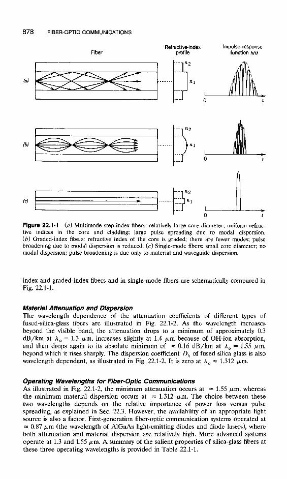
Figure 22.1-1 (a) Multimode step-index fibers: relatively large core diameter; uniform refrac- tive indices in the core and cladding; large pulse spreading due to modal dispersion. (b) Graded-index fibers: refractive index of the core is graded; there are fewer modes; pulse broadening due to modal dispersion is reduced. (c) Single-mode fibers: small core diameter; no modal dispersion; pulse broadening is due only to material and waveguide dispersion.
index and graded-index fibers and in single-mode fibers are schematically compared in Fig. 22.1-1.
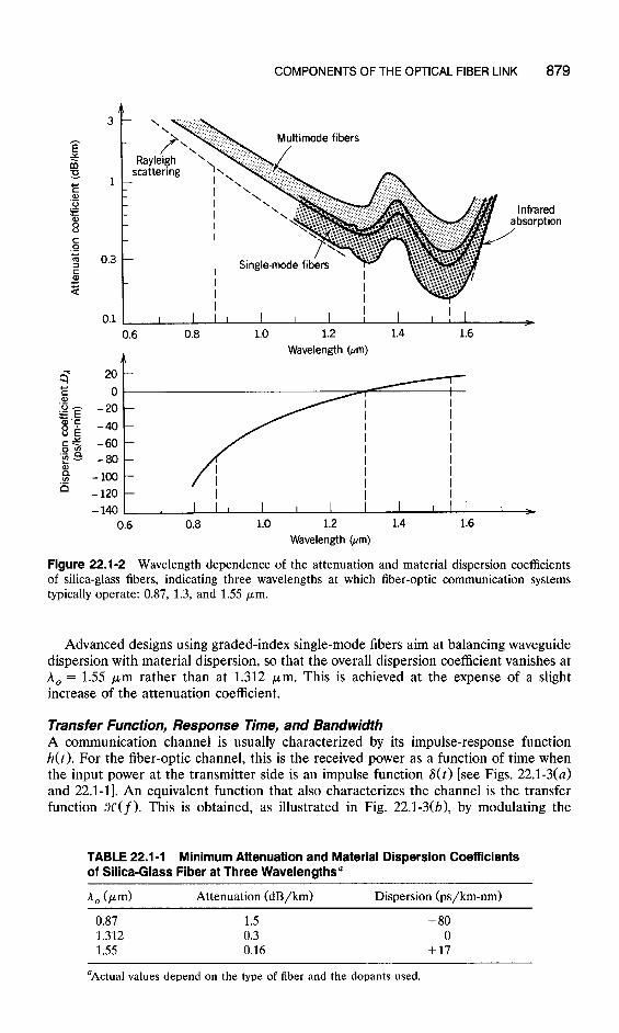
Material Attenuation and Dispersion The wavelength dependence of the attenuation coefficients of different types of fused-silica-glass fibers are illustrated in Fig. 22.1-2. As the wavelength increases beyond the visible band, the attenuation drops to a minimum of approximately 0.3 dB/km at A, = 1.3 ,um, increases slightly at 1.4 pm because of OH-ion absorption, and then drops again to its absolute minimum of = 0.16 dB/km at A, = 1.55 pm, beyond which it rises sharply. The dispersion coefficient D, of fused silica glass is also wavelength dependent, as illustrated in Fig. 22.1-2. It is zero at A, = 1.312 pm.
Operating Wavelengths for Fiber-Optic Communications As illustrated in Fig. 22.1-2, the minimum attenuation occurs at = 1.55 pm, whereas the minimum material dispersion occurs at = 1.312 pm. The choice between these two wavelengths depends on the relative importance of power loss versus pulse spreading, as explained in Sec. 22.3. However, the availability of an appropriate light source is also a factor. First-generation fiber-optic communication systems operated at = 0.87 pm (the wavelength of AlGaAs light-emitting diodes and diode lasers), where both attenuation and material dispersion are relatively high. More advanced systems operate at 1.3 and 1.55 pm. A summary of the salient properties of silica-glass fibers at these three operating wavelengths is provided in Table 22.1-1.
COMPONENTS OF THE OPTICAL FIBER LINK 879
Infrared absorption
/
I I 0.1 I I I I I I I
I 1 I I I >
0.6 0.8 1.0 1.2 1.4 1.6
Wavelength @m)
20
0 -20
-40
-60 -80
iii -100 - .- n / -120 -
- 140 I I I I I I I I \ 0.6 0.8 1.0 1.2 1.4 1.6
Wavelength km)
Figure 22.1-2 Wavelength dependence of the attenuation and material dispersion coefficients of silica-glass fibers, indicating three wavelengths at which fiber-optic communication systems typically operate: 0.87, 1.3, and 1.55 pm.
Advanced designs using graded-index single-mode fibers aim at balancing waveguide dispersion with material dispersion, so that the overall dispersion coefficient vanishes at A, = 1.55 pm rather than at 1.312 pm. This is achieved at the expense of a slight increase of the attenuation coefficient.
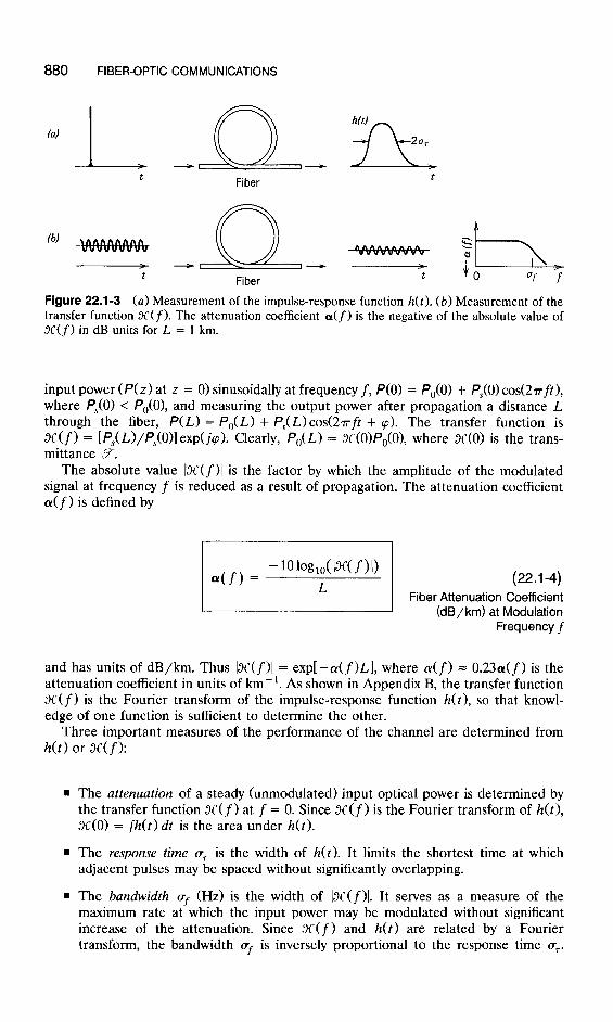
Transfer Function, Response Time, and Bandwidth A communication channel is usually characterized by its impulse-response function h(t). For the fiber-optic channel, this is the received power as a function of time when the input power at the transmitter side is an impulse function 8(t) [see Figs. 22.1-3(a) and 22.1-l]. An equivalent function that also characterizes the channel is the transfer function X(f). This is obtained, as illustrated in Fig. 22.1-3(b), by modulating the
TABLE 22.1-l Minimum Attenuation and Material Dispersion Coefficients of Silica-Glass Fiber at Three Wavelengths’
A, (pm) Attenuation (dB/km) Dispersion (ps/km-nm)
0.87 1.5 -80 1.312 0.3 0 1.55 0.16 +17
‘Actual values depend on the type of fiber and the dopants used.
880 FIBER-OPTIC COMMUNICATIONS
la) I -CL- t Fiber
fb) -m
= LL t Fiber
t
Figure 22.1-3 (a) Measurement of the impulse-response function h(t). (b) Measurement of the transfer function X(f). The attenuation coefficient a(f) is the negative of the absolute value of X(f) in dB units for L = 1 km.
input power (P(z) at z = 0) sinusoidally at frequency f, P(0) = P,(O) + Ps(0) cos(2~ft), where Ps(0) < P,(O), and measuring the output power after propagation a distance L through the fiber, P(L) = P,(L) + P,< L) cos(2rft + ~0). The transfer function is X(f) = [P,(L)/P,(O)] exp(j(p). Clearly, P,(L) = X(O)P,(O), where X(0) is the trans- mittance 7.
The absolute value IX(f)1 is the factor by which the amplitude of the modulated signal at frequency f is reduced as a result of propagation. The attenuation coefficient a(f) is defined by
and has units of dB/km. Thus Ix(f)1 = exp[ -a(f)L], where a(f) = 0.23a(f) is the attenuation coefficient in units of km-‘. As shown in Appendix B, the transfer function X(f) is the Fourier transform of the impulse-response function h(t), so that knowl- edge of one function is sufficient to determine the other.
Three important measures of the performance of the channel are determined from h(t) or X(f):
. The attenuation of a steady (unmodulated) input optical power is determined by the transfer function X(f) at f = 0. Since X(f) is the Fourier transform of h(t), X(O) = /h(t) dt is the area under h(t).
. The response time u7 is the width of h(t). It limits the shortest time at which adjacent pulses may be spaced without significantly overlapping.
. The bandwidth a- (Hz) is the width of Ix(f)l. It serves as a measure of the maximum rate at which the input power may be modulated without significant increase of the attenuation. Since x(f) and h(t) are related by a Fourier transform, the bandwidth Us is inversely proportional to the response time a7.
COMPONENTS OF THE OPTICAL FIBER LINK 881
Frequency f
:Hz
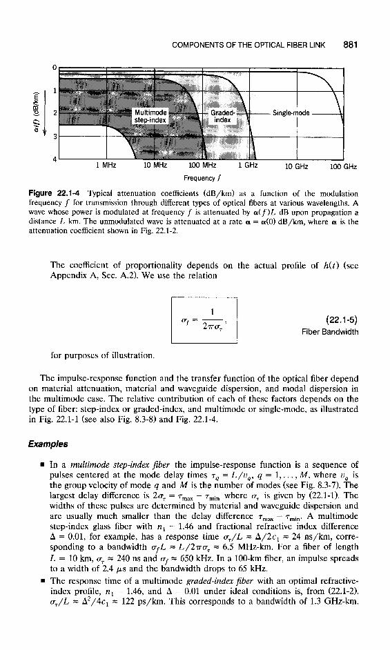
Figure 22.1-4 Typical attenuation coefficients (dB/km) as a function of the modulation frequency f for transmission through different types of optical fibers at various wavelengths. A wave whose power is modulated at frequency f is attenuated by (u( f )L dB upon propagation a distance L km. The unmodulated wave is attenuated at a rate (Y = 40) dB/km, where (Y is the attenuation coefficient shown in Fig. 22.1-2.
The coefficient of proportionality depends on the actual profile of h(t) (see Appendix A, Sec. A.2). We use the relation
1
*=T$ f (22.1-5) Fiber Bandwidth
for purposes of illustration.
The impulse-response function and the transfer function of the optical fiber depend on material attenuation, material and waveguide dispersion, and modal dispersion in the multimode case. The relative contribution of each of these factors depends on the type of fiber: step-index or graded-index, and multimode or single-mode, as illustrated in Fig. 22.1-1 (see also Fig. 8.3-8) and Fig. 22.1-4.
Examples
. In a multimode step-index fiber the impulse-response function is a sequence of pulses centered at the mode delay times r4 = L/v,, q = 1,. . . , M, where vq is the group velocity of mode q and M is the number of modes (see Fig. 8.3-7). The largest delay difference is 20, = r,, - 7,in where a7 is given by (22.1-1). The widths of these pulses are determined by material and waveguide dispersion and are usually much smaller than the delay difference r,, - 7,in. A multimode step-index glass fiber with n, = 1.46 and fractional refractive index difference A = 0.01, for example, has a response time a,/L = A/2c, = 24 ns/krn, corre- sponding to a bandwidth afL = L/27~u, = 6.5 MHz-km. For a fiber of length L = 10 km, a7 = 240 ns and af = 650 kHz. In a 100~km fiber, an impulse spreads to a width of 2.4 pus and the bandwidth drops to 65 kHz.
n The response time of a multimode graded-index fiber with an optimal refractive- index profile, n1 = 1.46, and A = 0.01 under ideal conditions is, from (22.1-2), UT/L = A2/4c, = 122 ps/km. This corresponds to a bandwidth of 1.3 GHz-km.
882 FIBER-OPTIC COMMUNICATIONS
Under these conditions, however, material dispersion depending on the spectral linewidth of the source.
may become important,
. For a sing&node fiber with a light source of spectral linewidth a;\ = 1 nm (from a typical single-mode laser) and a fiber dispersion coefficient D, = 1 ps/km-nm (for operatio n near h, = 1.3 pm), the response time given by (22-l-3) is o-*/L = 1 ps/km, corresponding to a bandwidth af = 159 GHz-km. A fiber of length 100 km has a response time 100 ps and bandwidth = 1.6 GHz.
Advanced Materials Several materials, with attenuation coefficients far smaller than that of silica glass, are being used in experimental optical systems in the mid-infrared region. These include heavy-metal fluoride glasses, halide-containing crystals, and chalcogenide glasses. For these materials, the infrared absorption band is located further in the infrared than in silica glass so that mid-infrared operation, with its attendant reduced Rayleigh scatter- ing (which decreases as l/At), is possible. Attenuations as small as 0.001 dB/km are expected to be achievable with fluoride-glass fibers operating at wavelengths in the 2 to 4 pm band. If these extremely low-loss materials are economically made into fibers, and if suitable semiconductor light sources are perfected for room-temperature opera- tion in the mid-infrared band, repeaterless transmission over distances of several thousand, instead of hundreds, of kilometers would become routine.
Fiber Amplifiers Erbium-doped silica fibers, serving as laser amplifiers (see Sec. 13.2C), are becoming increasingly important components of 1.55pm fiber-optic communication systems. These devices offer high-gain amplification (30 to 45 dB), with low noise, near the wavelength of lowest loss in silica glass. They are pumped by InGaAsP diode lasers (usually at 1.48 pm), and exhibit low insertion loss (< 0.5 dB) and polarization insensitivity. They are usually operated in the saturated regime and exhibit minimal crosstalk between different signals that are simutaneously transmitted through them.
An Er 3+-doped fiber amp lifier may be used as an optical-power amplifier placed directly at the output of the source laser, or as an optical preamplifier at the photodetector input (or both). It can also serve as an all-optical repeater, replacing the electronic repeaters that provide reshaping, retiming, and regeneration of the bits (e.g., those used in current long-haul undersea fiber-optic systems). All-optical repeaters are advantageous in that they offer increased gain and bandwidth, insensitivity to bit rate, and the ability to simultaneous amplify multiple optical channels.
Nonlinear Optical Properties of Fibers At high levels of power (tens of milliwatts), optical fibers exhibit nonlinear properties, which have a number of undesirable effects such as an increase of the pulse spreading in single-mode fibers, crosstalk between counter-propagating waves used in two-way communications, and crosstalk between waves of different wavelengths used in wave- length-division multiplexing. However, the nonlinear properties of fibers may be harnessed for useful applications. Nonlinear dispersion (dependence of the phase velocity on the intensity) may be adjusted to compensate for chromatic dispersion in the fiber. The result is spreadless pulses known as optical solitons (see Sec. 19.8). The gain provided by a fiber amplifier can be used to compensate for the fiber attenuation so that ideally the pulses suffer no attenuation and no spreading. Nonlinear interac- tions can also be used to provide gain, but the properties of such amplifiers are generally inferior to those of laser amplifiers such as Er3+:silica fiber.
COMPONENTS OF THE OPTICAL FIBER LINK 883
B. Sources for Optical Transmitters
The basic requirements for the light sources used in optical communication systems depend on the nature of the intended application (long-haul communication, local-area network, etc.). The main features are:
9 Power. The source power must be sufficiently high so that after transmission through the fiber the received signal is detectable with the required accuracy.
n Speed. It must be possible to modulate the source power at the desired rate. . Linewidth. The source must have a narrow spectral linewidth so that the effect of
chromatic dispersion in the fiber is minimized. n Noise. The source must be free of random fluctuations. This requirement is
particularly strict for coherent communication systems. n Other features include ruggedness, insensitivity to environmental changes such as
temperature, reliability, low cost, and long lifetime.
Both light-emitting diodes (LEDs) and laser diodes are used as sources in fiber-optic communication systems. These devices are discussed in Chap. 16.
Laser diodes have the advantages of high power (tens of mW), high speeds (in the GHz region), and narrow spectral width. However, they are sensitive to temperature variations. Multimode diode lasers suffer from partition noise, i.e., random distribution of the laser power among the modes. When combined with chromatic dispersion in the fiber, this leads to random intensity fluctuations and reshaping of the transmitted pulses. Laser diodes also suffer from frequency chirping, i.e., variation of the laser frequency as the optical power is modulated. Chirping results from changes of the refractive index that accompany changes of the charge-carrier concentrations as the injected current is altered. Significant advances in semiconductor laser technology in recent years have resulted in many improvements and in considerable increase of their reliability and lifetime.
Light-emitting diodes are fabricated in two basic structures: surface emitting and edge emitting. Surface-emitting diodes have the advantages of ruggedness, reliability, lower cost, long lifetime, and simplicity of design. However, their basic limitation is their relatively broader linewidth (more than 100 nm in the band 1.3 to 1.6 pm). When operated at their maximum power, modulation frequencies up to 100 Mb/s are possible, but higher speeds (up to 500 Mb/s) can only be achieved at reduced powers. The edge-emitting diode has a structure similar to the diode laser (with the reflectors removed). It produces more power output with relatively narrower spectral linewidth, at the expense of complexity.
Sources at 0.87 pm AlGaAs light-emitting diodes and AlGaAs/GaAs double-heterostructure and quan- tum-well laser diodes have been used at this wavelength. Surface-emitting LEDs are used extensively.
Sources at 1.3 and 7.55 pm InGaAsP LEDs have been used in this band with moderate speeds and powers. Single-mode systems make use of InGaAsP/InP double-heterostructure lasers together with single-mode fibers. The requirement for a narrow spectral linewidth is not as crucial at 1.3 pm since material dispersion is minimal. At 1.55 pm, however, it is important to use sources with narrow linewidths because of the presence of material dispersion. A number of technologies are available for providing single-longitudinal- mode lasers (single-frequency lasers) that are stable at high speeds of modulation (see
884 FIBER-OPTIC COMMUNICATIONS
Sec. 16.3E). These include external-cavity lasers, distributed feedback (DFB) and distributed Bragg-reflector (DBR) lasers capable of providing spectral linewidths of 5 to 100 MHz at a few mW of output power with modulation rates exceeding 20 GHz, and cleaved-coupled-cavity (C3) lasers which promise linewidths as low as 1 MHz (but are subject to thermal drift).
DFB lasers are probably the most commonly used. Current modulation can be employed since the frequency chirp can be made sufficiently small. DFB lasers with multiple sections and/or multiple electrodes are under development; these should provide further improvements in performance. Quantum-well lasers, in particular InGaAs strained-layer quantum-well lasers (see Sec. 16.3G), are highly promising. These devices offer lower thresholds and larger bandwidths than their lattice-matched cousins (theoretical calculations show that thresholds as low as 50 A/cm*, and bandwidths as high as 100 GHz, are possible). The prospects for quantum-wire and quantum-dot lasers (see Sec. 15.1G) lie further in the future.
Sources at Longer Wavelengths Interest in wavelengths longer than 1.55 pm is engendered by the development of low-loss fibers in the 2- to 4-pm wavelength band. Laser diodes that can be operated at room temperature at these wavelengths are being developed. Double-heterostructure InGaAsSb/AlGaAsSb lasers (lattice matched to a GaSb substrate), as an example, can be operated at A, = 2.27 pm at T = 300 K (so far only in the pulsed mode, however), with a threshold current density = 1500 A/cm *, differential quantum efficiency = 0.5, and output power = 2 W. Emission wavelengths from 1.8 to 4.4 ,um can potentially be obtained for the range of InGaAsSb compositions that can be lattice matched to GaSb.
C. Detectors for Optical Receivers
A comprehensive discussion of semiconductor photon detectors is provided in Chap. 17. Two types of detectors are commonly used in optical communication systems: the p-i-n photodiode and the avalanche photodiode (APD). The APD has the advantage of providing gain before the first electronic amplification stage in the receiver, thereby reducing the detrimental effects of circuit noise. However, the gain mechanism itself introduces noise and has a finite response time, which may reduce the bandwidth of the receiver. Furthermore, APDs require a high-voltage supply and more complicated circuitry to compensate for their sensitivity to temperature fluctuations. The signal-to- noise ratio and the sensitivity of receivers using p-i-n photodiodes and APDs are discussed in Sets. 17.5 and 22.4.
Detectors at 0.87 pm Silicon p-i-n photodiodes and APDs are used at these wavelengths. In state-of-the-art preamplifiers, silicon APDs enjoy a lo-to-15-dB sensitivity advantage over silicon p-i-n photodiodes because their internal gain makes the noise of the preamplifier relatively less important. The sensitivity of Si APDs at bit rates up to several hundred Mb/s corresponds to about 100 photons/bit. (For a discussion of receiver sensitivity, see Sec. 22.4.)
Detectors at 1.3 and 7.55 pm Silicon is not usable in this region because its bandgap is greater than the photon energy. Germanium and InGaAs p-i-n photodiodes are both used; InGaAs is preferred because it has greater thermal stability and lower dark noise. Typical InGaAs p-i-n photodiodes have quantum efficiencies ranging from 0.5 to 0.9, responsivities = 1 A/W, and response times that are in the tens of ps (corresponding to bandwidths up to
COMPONENTS OF THE OPTICAL FIBER LINK 885
n-: In0.53Ga0.&s (Absorption)
n: ‘n0.7Ga0.3~0.65P0.35 Wading)
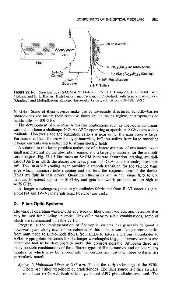
Figure 22.1-5 Structure of an SAGM APD. (Adapted from J. C. Campbell, A. G. Dentai, W. S. Holden, and B. L. Kasper, High-Performance Avalanche Photodiode with Separate Absorption, ‘Grading’, and Multiplication Regions, Electronics Letters, vol. 19, pp. 818-820, 1983.)
60 GHz). Some of these devices make use of waveguide structures. Schottky-barrier photodiodes are faster; their response times are in the ps regime, corresponding to bandwidths = 100 GHz.
The development of low-noise APDs (for applications such as fiber-optic communi- cations) has been a challenge. InGaAs APDs operating at speeds = 2 Gb/s are widely available. However since the ionization ratio I: is near unity, the gain noise is large. Furthermore, like all narrow bandgap materials, InGaAs suffers from large tunneling leakage currents when subjected to strong electric fields.
A solution to this latter problem makes use of a heterostructure of two materials-a small gap material for the absorption region, and a large-gap material for the multipli- cation region. Fig. 22.1-5 illustrates an SAGM (separate absorption, grading, multipli- cation) APD in which the absorption takes place in InGaAs and the multiplication in InP. The InGaAsP grading layer provides a smooth transition for the valence band edge which minimizes hole trapping and shortens the response time of the device. Holes multiply in this device. Quantum efficiencies are in the range 0.75 to 0.9, bandwidths extend up to = 10 GHz, and gain-bandwidth products are as high as = 75 GHz.
At longer wavelengths, junction photodiodes fabricated from II-VI materials (e.g., HgCdTe) and IV-VI materials (e.g., PbSnTe) are useful.
D. Fiber-Optic Systems
The various operating wavelengths and types of fibers, light sources, and detectors that may be used for building an optical link offer many possible combinations, some of which are summarized in Table 22.1-2.
Progress in the implementation of fiber-optic systems has generally followed a downward path along each of the columns of this table, toward longer wavelengths: from multimode to single-mode fibers, from LEDs to lasers, and from photodiodes to APDs. Appropriate materials for the longer wavelengths (e.g., quaternary sources and detectors) had to be developed to make this progress possible. Although there are many possible combinations of the different types of fibers, sources, and detectors, any number of which may be appropriate for certain applications, three systems are particularly noted:
System 1: Multimode Fibers at 0.87 pm. This is the early technology of the 1970s. Fibers are either step-index or graded-index. The light source is either an LED or a laser (AlGaAs). Both silicon p-i-n and APD photodiodes are used. The
886 FIBER-OPTIC COMMUNICATIONS
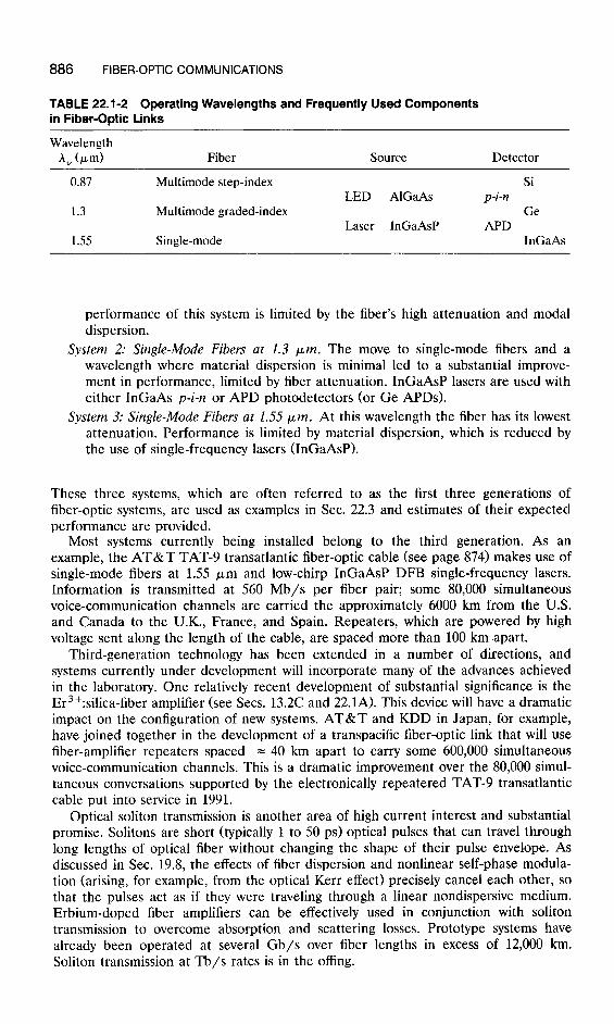
TABLE 22.1-2 Operating Wavelengths and Frequently Used Components in Fiber-Optic Links
Wavelength A, (pm> Fiber Source Detector
0.87 Multimode step-index
1.3 Multimode graded-index
1.55 Single-mode
LED AlGaAs
Laser InGaAsP
Si p-i-n
Ge APD
InGaAs
performance of this system is limited by the fiber’s high attenuation and modal dispersion.
System 2: Single-Mode Fibers at 1.3 pm. The move to single-mode fibers and a wavelength where material dispersion is minimal led to a substantial improve- ment in performance, limited by fiber attenuation. InGaAsP lasers are used with either InGaAs p-i-n or APD photodetectors (or Ge APDs).
System 3: Single-Mode Fibers at 1.55 pm. At this wavelength the fiber has its lowest attenuation. Performance is limited by material dispersion, which is reduced by the use of single-frequency lasers (InGaAsP).
These three systems, which are often referred to as the first three generations of fiber-optic systems, are used as examples in Sec. 22.3 and estimates of their expected performance are provided.
Most systems currently being installed belong to the third generation. As an example, the AT&T TAT-9 transatlantic fiber-optic cable (see page 874) makes use of single-mode fibers at 1.55 pm and low-chirp InGaAsP DFB single-frequency lasers. Information is transmitted at 560 Mb/s per fiber pair; some 80,000 simultaneous voice-communication channels are carried the approximately 6000 km from the U.S. and Canada to the U.K., France, and Spain. Repeaters, which are powered by high voltage sent along the length of the cable, are spaced more than 100 km apart.
Third-generation technology has been extended in a number of directions, and systems currently under development will incorporate many of the advances achieved in the laboratory. One relatively recent development of substantial significance is the Er3+:silica-fiber amplifier (see Sets. 13.2C and 22.1A). This device will have a dramatic impact on the configuration of new systems. AT&T and KDD in Japan, for example, have joined together in the development of a transpacific fiber-optic link that will use fiber-amplifier repeaters spaced = 40 km apart to carry some 600,000 simultaneous voice-communication channels. This is a dramatic improvement over the 80,000 simul- taneous conversations supported by the electronically repeatered TAT-9 transatlantic cable put into service in 1991.
Optical soliton transmission is another area of high current interest and substantial promise. Solitons are short (typically 1 to 50 ps) optical pulses that can travel through long lengths of optical fiber without changing the shape of their pulse envelope. As discussed in Sec. 19.8, the effects of fiber dispersion and nonlinear self-phase modula- tion (arising, for example, from the optical Kerr effect) precisely cancel each other, so that the pulses act as if they were traveling through a linear nondispersive medium. Erbium-doped fiber amplifiers can be effectively used in conjunction with soliton transmission to overcome absorption and scattering losses. Prototype systems have already been operated at several Gb/s over fiber lengths in excess of 12,000 km. Soliton transmission at Tb/s rates is in the offing.
MODULATION, MULTIPLEXING, AND COUPLING 887
All of the systems described above make use of direct detection, in which only the signal light illuminates the photodetector. Fourth-generation systems make use of coherent detection (see Sec. 22.5), in which a locally generated source of light (the local oscillator) illuminates the photodetector along with the signal. Erbium-doped fiber amplifiers are also useful in conjunction with heterodyne systems. The use of coherent detection in a fiber-optic communication system improves system performance; how- ever, this comes at the expense of increased complexity. As a result, the commercial implementation of coherent systems has lagged behind that of direct-detection systems.
22.2 MODULATION, MULTIPLEXING, AND COUPLING
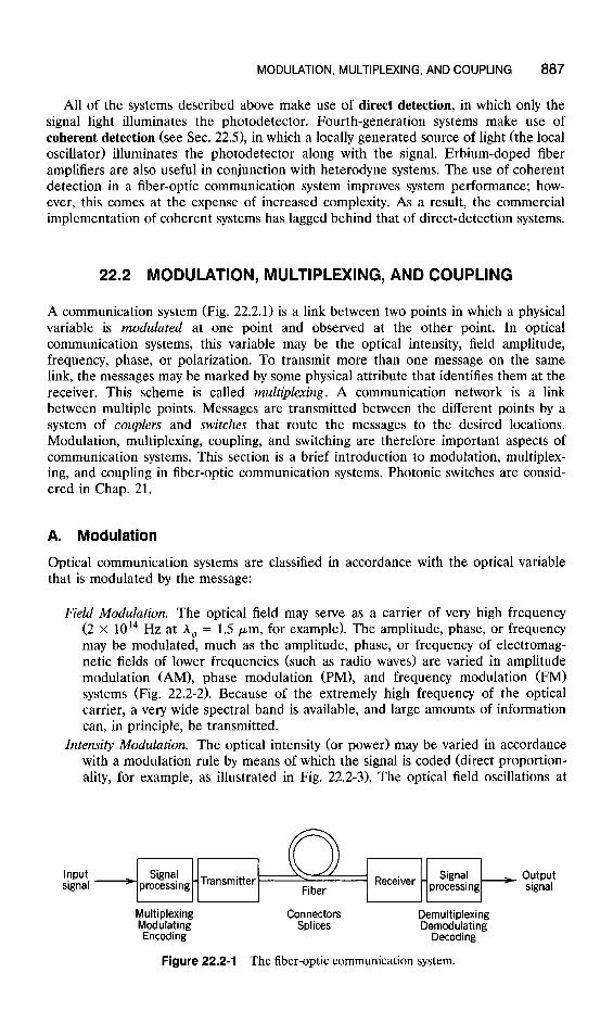
A communication system (Fig. 22.2.1) is a link between two points in which a physical variable is modulated at one point and observed at the other point. In optical communication systems, this variable may be the optical intensity, field amplitude, frequency, phase, or polarization. To transmit more than one message on the same link, the messages may be marked by some physical attribute that identifies them at the receiver. This scheme is called multiplexing. A communication network is a link between multiple points. Messages are transmitted between the different points by a system of couplers and switches that route the messages to the desired locations. Modulation, multiplexing, coupling, and switching are therefore important aspects of communication systems. This section is a brief introduction to modulation, multiplex- ing, and coupling in fiber-optic communication systems. Photonic switches are consid- ered in Chap. 21.
A. Modulation
Optical communication systems are that is modulated by the message:
classified in accordance with the optical variable
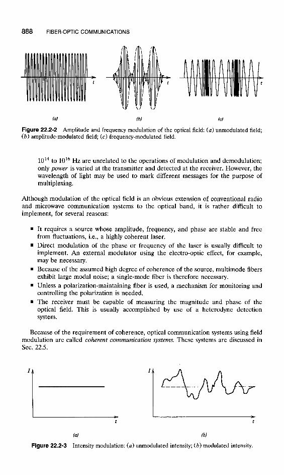
Field Modulation. The optical field may serve as a carrier of very high frequency (2 x 10¹⁴ Hz at h, = 1.5 pm, for example). The amplitude, phase, or frequency may be modulated, much as the amplitude, phase, or frequency of electromag- netic fields of lower frequencies (such as radio waves) are varied in amplitude modulation (AM), phase modulation (PM), and frequency modulation (FM) systems (Fig. 22.2-2). Because of the extremely high frequency of the optical carrier, a very wide spectral band is available, and large amounts of information can, in principle, be transmitted.
Intensity Modulation. The optical intensity (or power) may be varied in accordance with a modulation rule by means of which the signal is coded (direct proportion- ality, for example, as illustrated in Fig. 22.2-3). The optical field oscillations at
Input signal
_ Signal - processing -Transmitter a Receiver - Signal --b
Fiber processing -
Multiplexing Connectors ME&d;;;rgg Splices
Demultiplexing Demodulating
Decoding
output signal
Figure 22.2-l The fiber-optic communication system.
888 FIBER-OPTIC COMMUNICATIONS
fb) fc)
Figure 22.2-2 Amplitude and frequency modulation of the optical field: (a) unmodulated field; (b) amplitude-modulated field; (c) frequency-modulated field.
1014 to 1016 Hz are unrelated to the operations of modulation and demodulation; only power is varied at the transmitter and detected at the receiver. However, the wavelength of light may be used to mark different messages for the purpose of multiplexing.
Although modulation of the optical field is an obvious extension of conventional radio and microwave communication systems to the optical band, it is rather difficult to implement, for several reasons:
9 It requires a source whose amplitude, frequency, and phase are stable and free from fluctuations, i.e., a highly coherent laser.
. Direct modulation of the phase or frequency of the laser is usually difficult to implement. An external modulator using the electro-optic effect, for example, may be necessary.
. Because of the assumed high degree of coherence of the source, multimode fibers exhibit large modal noise; a single-mode fiber is therefore necessary.
. Unless a polarization-maintaining fiber is used, a mechanism for monitoring and controlling the polarization is needed.
. The receiver must be capable of measuring the magnitude and phase of the optical field. This is usually accomplished by use of a heterodyne detection system.
Because of the requirement of coherence, optical communication systems using field modulation are called coherent communication systems. These systems are discussed in Sec. 22.5.
I
-t
I
fb)
Figure 22.2-3 Intensity modulation: (a) unmodulated intensity; (b) modulated intensity.
MODULATION, MULTIPLEXING, AND COUPLING 889
t
Signal f >4kHZ
PCM signal 1
i
-j j+- 15.625 ,us 64 kbls
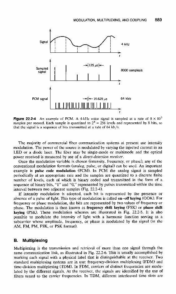
Figure 22.2-4 An example of PCM. A 4-kHz voice signal is sampled at a rate of 8 X lo3 samples per second. Each sample is quantized to 2s = 256 levels and represented by 8 bits, so that the signal is a sequence of bits transmitted at a rate of 64 kb/s.
The majority of commercial fiber communication systems at present use intensity modulation. The power of the source is modulated by varying the injected current in an LED or a diode laser. The fiber may be single-mode or multimode and the optical power received is measured by use of a direct-detection receiver.
Once the modulation variable is chosen (intensity, frequency, or phase), any of the conventional modulation formats (analog, pulse, or digital) can be used. An important example is pulse code modulation (PCM). In PCM the analog signal is sampled periodically at an appropriate rate and the samples are quantized to a discrete finite number of levels, each of which is binary coded and transmitted in the form of a sequence of binary bits, “1” and “0,” represented by pulses transmitted within the time interval between two adjacent samples (Fig. 22.2-4).
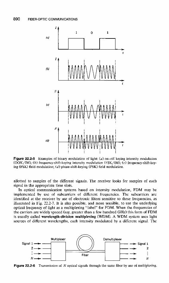
If intensity modulation is adopted, each bit is represented by the presence or absence of a pulse of light. This type of modulation is called on-off keying (OOK). For frequency or phase modulation, the bits are represented by two values of frequency or phase. The modulation is then known as frequency shift keying (FSK) or phase shift keying (PSK). These modulation schemes are illustrated in Fig. 22.2-5. It is also possible to modulate the intensity of light with a harmonic function serving as a subcarrier whose amplitude, frequency, or phase is modulated by the signal (in the AM, FM, PM, FSK, or PSK format).
B. Multiplexing
Multiplexing is the transmission and retrieval of more than one signal through the same communication link, as illustrated in Fig. 22. 2-6. This is usually accomplished by marking each signal with a physical label that is distinguishable at the receiver. Two standard multiplexing systems are in use: frequency-division multiplexing (FDM) and time-division multiplexing (TDM). In FDM, carriers of distinct frequencies are modu- lated by the different signals. At the receiver, the signals are identified by the use of filters tuned to the carrier frequencies. In TDM, different interleaved time slots are
890 FIBER-OPTIC COMMUNICATIONS
I
t 1 0 1
lb)
(4
(4
Figure 22.2-5 Examples of binary modulation of light: (a) on-off keying intensity modulation (OOK/IM); (b) frequency-shift-keying intensity modulation (FSK/IM); (c) frequency-shift-key- ing (FSK) field modulation; (d) phase-shift-keying (PSK) field modulation.
allotted to samples of the different signals. The receiver looks for samples of each signal in the appropriate time slots.
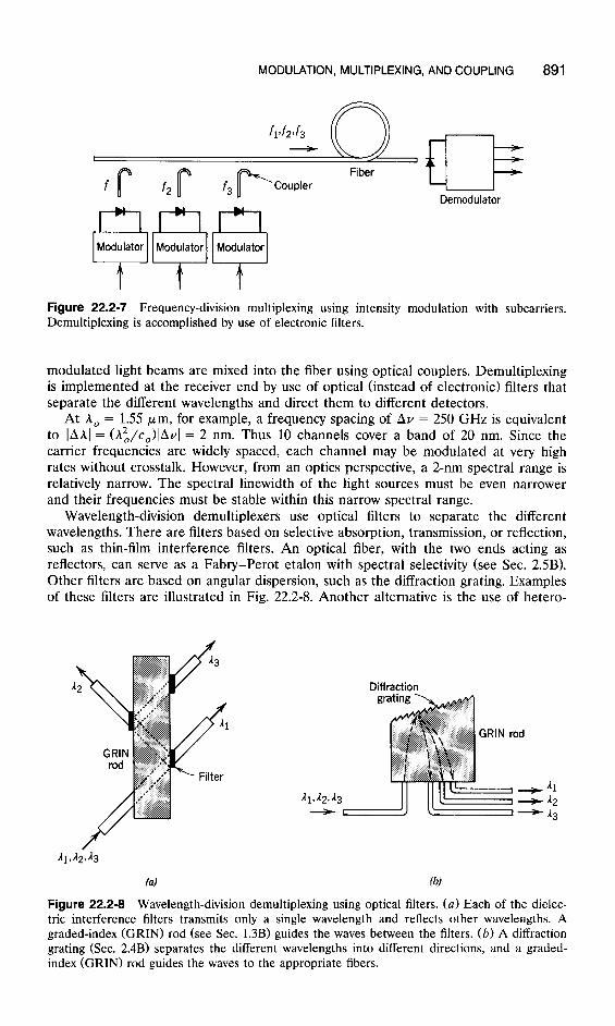
In optical communication systems based on intensity modulation, FDM may be implemented by use of subcarriers of different frequencies. The subcarriers are identified at the receiver by use of electronic filters sensitive to these frequencies, as illustrated in Fig. 22.2-7. It is also possible, and more sensible, to use the underlying optical frequency of light as a multiplexing “label” for FDM. When the frequencies of the carriers are widely spaced (say, greater than a few hundred GHz) this form of FDM is usually called wavelength-division multiplexing (WDM). A WDM system uses light sources of different wavelengths, each intensity modulated by a different signal. The
Signal 1 - 2-
w Signal 1 2 . . .
N
Figure 22.2-6 Transmission of N optical signals through the same fiber by use of multiplexing.
MODULATION, MULTIPLEXING, AND COUPLING 891
Fiber
si?? Modulator Modulator Modulator
Figure 22.2-7 Frequency-division multiplexing using intensity modulation with subcarriers. Demultiplexing is accomplished by use of electronic filters.
modulated light beams are mixed into the fiber using optical couplers. Demultiplexing is implemented at the receiver end by use of optical (instead of electronic) filters that separate the different wavelengths and direct them to different detectors.
At A, = 1.55 pm, for example, a frequency spacing of AV = 250 GHz is equivalent to [AAl = (/42,/c,>lAvl = 2 nm. Thus 10 channels cover a band of 20 nm. Since the carrier frequencies are widely spaced, each channel may be modulated at very high rates without crosstalk. However, from an optics perspective, a 2-nm spectral range is relatively narrow. The spectral linewidth of the light sources must be even narrower and their frequencies must be stable within this narrow spectral range.
Wavelength-division demultiplexers use optical filters to separate the different wavelengths. There are filters based on selective absorption, transmission, or reflection, such as thin-film interference filters. An optical fiber, with the two ends acting as reflectors, can serve as a Fabry-Perot etalon with spectral selectivity (see Sec. 2SB). Other filters are based on angular dispersion, such as the diffraction grating. Examples of these filters are illustrated in Fig. 22.2-8. Another alternative is the use of hetero-
Diff t-action
(al (b)
Figure 22.2-8 Wavelength-division demultiplexing using optical filters. (a) Each of the dielec- tric interference filters transmits only a single wavelength and reflects other wavelengths. A graded-index (GRIN) rod (see Sec. 1.3B) guides the waves between the filters. (b) A diffraction grating (Sec. 2.4B) separates the different wavelengths into different directions, and a graded- index (GRIN) rod guides the waves to the appropriate fibers.
892 FIBER-OPTIC COMMUNICATIONS
dyne detection. A wavelength-multiplexed optical signal with carrier frequencies VI, v’2, * * * is mixed with a local oscillator of frequency vL and detected. The photocur- rent carries the signatures of the different carriers at the beat frequencies fi = vl - vL, f2 = v2 - VL, . . . . These frequencies are then separated using electronic filters (see Sec. 22.5A).
C. Couplers
In addition to the transmitter, the fiber link, and the receiver, a communication system uses couplers and switches which direct the light beams that represent the various signals to their appropriate destinations. Couplers always operate on the incoming signals in the same manner. Switches are controllable couplers that can be modified by an external command. Photonic switches are described in Chap. 21.
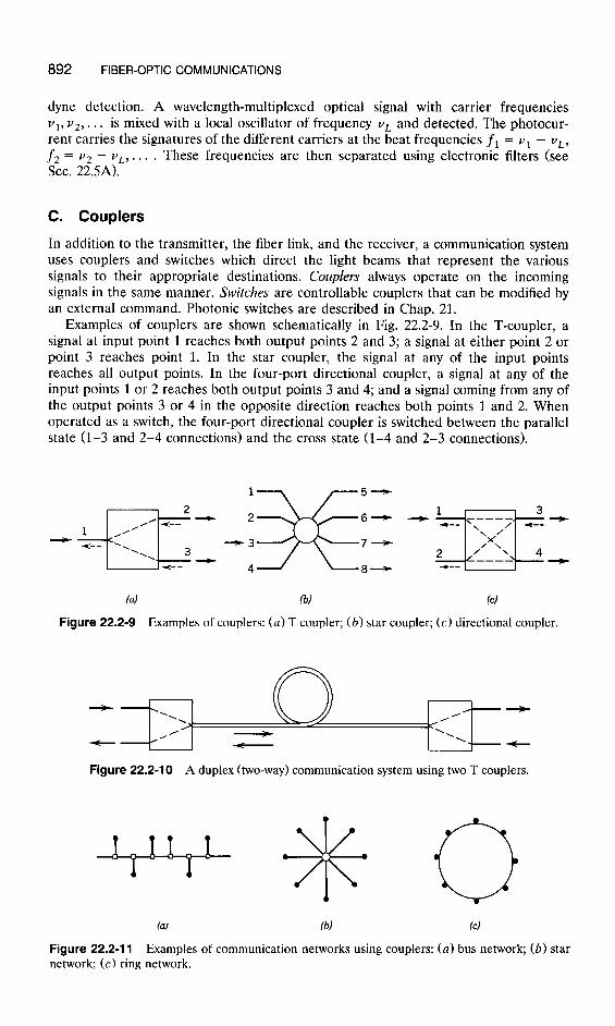
Examples of couplers are shown schematically in Fig. 22.2-9. In the T-coupler, a signal at input point 1 reaches both output points 2 and 3; a signal at either point 2 or point 3 reaches point 1. In the star coupler, the signal at any of the input points reaches all output points. In the four-port directional coupler, a signal at any of the input points 1 or 2 reaches both output points 3 and 4; and a signal coming from any of the output points 3 or 4 in the opposite direction reaches both points 1 and 2. When operated as a switch, the four-port directional coupler is switched between the parallel state (l-3 and 2-4 connections) and the cross state (1-4 and 2-3 connections).
(al (b) (4
Figure 22.2-9 Examples of couplers: (a) T coupler; (b) star coupler; (c) directional coupler.
Figure 22.2-10 A duplex (two-way) communication system using two T couplers.
(a) fb) (4
Figure 22.2-l 1 Examples of communication networks using couplers: (a) bus network; (b) star network; (c) ring network.
SYSTEM PERFORMANCE 893
1 1 Light source
‘Lens z Beams’plitter
(a)
2 4
(4
\ Beamsplitter
film
Mixing rod
Fibers
fb)
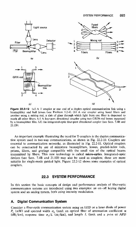
Figure 22.2-12 (a) A T coupler at one end of a duplex optical communication link using a beamsplitter and ball lenses (see Problem 1.2-4). (b) A star coupler using fused fibers and another using a mixing rod, a slab of glass through which light from one fiber is dispersed to reach all other fibers. (c) A four-port directional coupler using two GRIN-rod lenses separated by a beamsplitter film. (d) An integrated-optic four-port directional coupler (see Sets. 7.4B and 21.1B).
An important example illustrating the need for T-couplers is the duplex communica- tion system used in two-way communications, as shown in Fig. 22.2-10. Couplers are essential to communication networks, as illustrated in Fig. 22.2-11. Optical couplers can be constructed by use of miniature beamsplitters, lenses, graded-index rods, prisms, filters, and gratings compatible with the small size of the optical beams transmitted by fibers. This new technology is called micro-optics. Integrated-optic devices (see Sets. 7.4B and 21.1B) may also be used as couplers; these are more suitable for single-mode guided light. Figure 22.2-12 shows some examples of optical couplers.
22.3 SYSTEM PERFORMANCE
In this section the basic concepts of design and performance analysis of fiber-optic communication systems are introduced using two examples: an on-off keying digital system and an analog system, both using intensity modulation.
A. Digital Communication System
Consider a fiber-optic communication system using an LED or a laser diode of power P, (mW) and spectral width aA (nm); an optical fiber of attenuation coefficient (Y (dB/km), response time uJL (ns/km), and length L (km); and a p-i-n or APD
894 FIBER-OPTIC COMMUNICATIONS
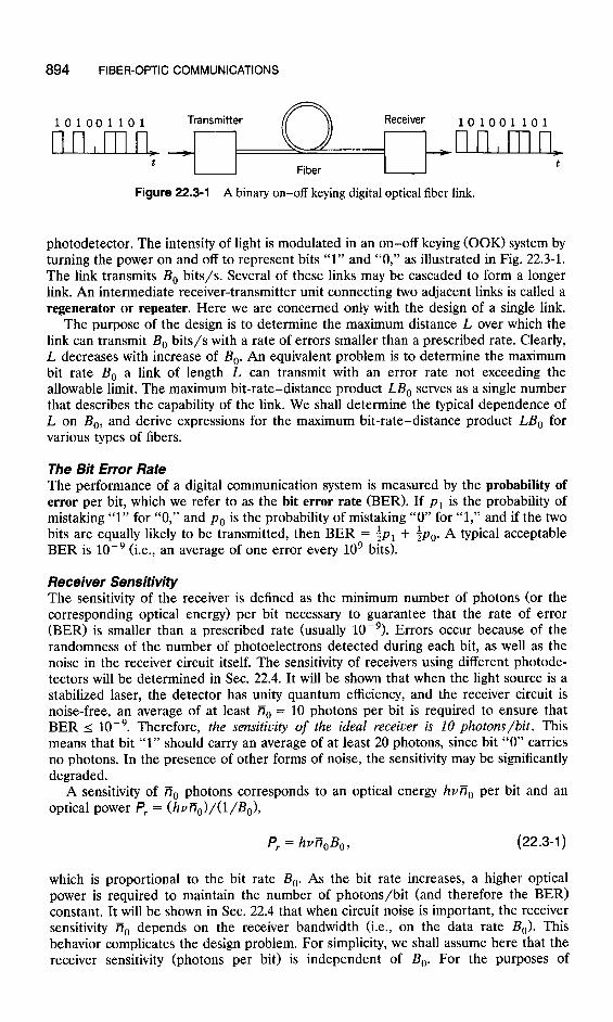
Figure 22.3-l A binary on-off keying digital optical fiber link.
photodetector. The intensity of light is modulated in an on-off keying (OOK) system by turning the power on and off to represent bits “1” and “0,” as illustrated in Fig. 22.3-l. The link transmits B, bits/s. Several of these links may be cascaded to form a longer link. An intermediate receiver-transmitter unit connecting two adjacent links is called a regenerator or repeater. Here we are concerned only with the design of a single link.
The purpose of the design is to determine the maximum distance L over which the link can transmit B, bits/s with a rate of errors smaller than a prescribed rate. Clearly, L decreases with increase of B,. An equivalent problem is to determine the maximum bit rate B, a link of length L can transmit with an error rate not exceeding the allowable limit. The maximum bit-rate-distance product LB, serves as a single number that describes the capability of the link. We shall determine the typical dependence of L on B,, and derive expressions for the maximum bit-rate-distance product LB, for various types of fibers.
The Bit Error Rate The performance of a digital communication system is measured by the probability of error per bit, which we refer to as the bit error rate (BER). If p1 is the probability of mistaking “1” for “0,” and p,, is the probability of mistaking “0” for “1,” and if the two bits are equally likely to be transmitted, then BER = $p1 + $pO. A typical acceptable BER is 10m9 (i.e., an average of one error every lo9 bits).
Receiver Sensitivity The sensitivity of the receiver is defined as the minimum number of photons (or the corresponding optical energy) per bit necessary to guarantee that the rate of error (BER) is smaller than a prescribed rate (usually 10V9). Errors occur because of the randomness of the number of photoelectrons detected during each bit, as well as the noise in the receiver circuit itself. The sensitivity of receivers using different photode- tectors will be determined in Sec. 22.4. It will be shown that when the light source is a stabilized laser, the detector has unity quantum efficiency, and the receiver circuit is noise-free, an average of at least A, = 10 photons per bit is required to ensure that BER I 10e9. Therefore, the sensitivity of the ideal receiver is 10 photons/bit. This means that bit “1” should carry an average of at least 20 photons, since bit “0” carries no photons. In the presence of other forms of noise, the sensitivity may be significantly degraded.
A sensitivity of A, photons corresponds to an optical energy hvfiO per bit and an optical power P, = (hv77,)/(l/B,),
P, = hvAOBO, (22.3-l)
which is proportional to the bit rate B,. As the bit rate increases, a higher optical power is required to maintain the number of photons/bit (and therefore the BER) constant. It will be shown in Sec. 22.4 that when circuit noise is important, the receiver sensitivity A, depends on the receiver bandwidth (i.e., on the data rate B,). This behavior complicates the design problem. For simplicity, we shall assume here that the receiver sensitivity (photons per bit) is independent of B,. For the purposes of
SYSTEM PERFORMANCE 895
illustration we shall use the nominal receiver sensitivities of ii, = 300 photons per bit for receivers operating at A, = 0.87 pm and 1.3 pm, and R, = 1000 photons per bit for receivers operating at A, = 1.55 pm.
Design Strategy Once we know the minimum power required at the receiver, the power of the source, and the fiber attenuation per kilometer, a power budget may be prepared from which the maximum fiber length is determined. We must also prepare a budget for the pulse spreading that results from dispersion in the fiber. If the width a7 of the received pulses exceeds the bit time interval l/B,, adjacent pulses overlap and cause intersym- bol interference, which increases the error rates. There are therefore two conditions for the acceptable operation of the link:
. The received power must be at least equal to the receiver power sensitivity P,.. A margin of 6 dB above Pr is usually specified.
n The received pulse width (TV must not exceed a prescribed fraction of the bit time interval l/B,.
If the bit rate B, is fixed and the link length L is increased, two situations leading to performance degradation may occur: The received power becomes smaller than the receiver power sensitivity Pr, or the received pulses become wider than the bit time l/B,. If the former situation occurs first, the link is said to be attenuation limited. If the latter occurs first, the link is said to be dispersion limited.
Attenuation-Limited Performance Attenuation-limited performance is assessed by preparing a power budget. Since fiber attenuation is measured in dB units, it is convenient to also measure power in dB units. Using 1 mW as a reference, dBm units are defined by
9 = lOlog,() P, PinmW; 9indBm.
I 1
For example, P = 0.1 mW, 1 mW, and 10 mW correspond to 9 = - 10 dBm, 0 dBm, and 10 dBm, respectively. In these logarithmic units, power losses are additive instead of multiplicative.
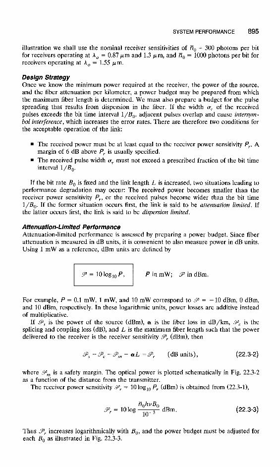
If LZ@~ is the power of the source (dBm), Q is the fiber loss in dB/km, CYC is the splicing and coupling loss (dB), and L is the maximum fiber length such that the power delivered to the receiver is the receiver sensitivity 9,. (dBm), then
Ps -cYc --Ym - CUL =9$ (dB units), (22.3-2)
where L?J~ is a safety margin. The optical power is plotted schematically in Fig. 22.3-2 as a function of the distance from the transmitter.
The receiver power sensitivity L?~ = 10 log,, P, (dBm) is obtained from (22.3-l),
iiohvBo Pr = lOlog-
1o-3 dBm . (22.3-3)
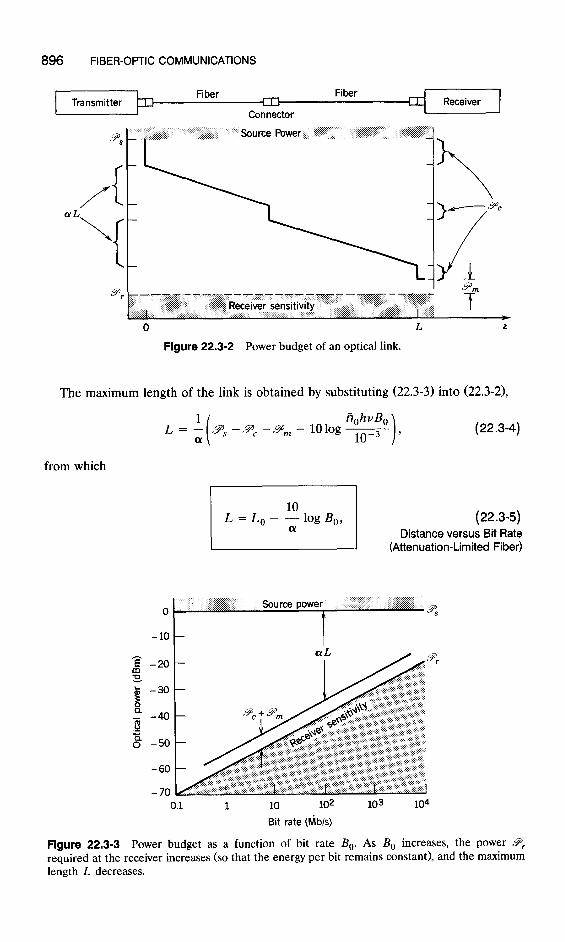
Thus L?~ increases logarithmically with B,, and the power budget must be adjusted for each B, as illustrated in Fig. 22.3-3.
896 FIBER-OPTIC COMMUNICATIONS
Transmitter Connector
Source Power
9 I 9 m r--7----- --*----- ---------.v.-----
0 L
Figure 22.3-2 Power budget of an optical link.
The maximum length of the link is obtained by substituting (22.3-3) into (22.3-2),
- lOlog- (22.3-4)
from which
0 Source power ,, ,. ,,
t 3
0.1 1 10 102 103 104 Bit rate &lb/s)
Figure 22.3-3 Power budget as a function of bit rate B,. As B, increases, the power ?Fr required at the receiver increases (so that the energy per bit remains constant), and the maximum length L decreases.
SYSTEM PERFORMANCE a97
1 I
10 100
Bit rate BO (Mb/s)
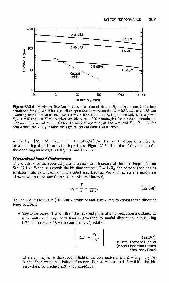
Figure 22.3-4 Maximum fiber length L as a function of bit rate B, under attenuation-limited conditions for a fused silica glass fiber operating at wavelengths A, = 0.87, 1.3, and 1.55 ,um assuming fiber attenuation coefficients LY = 2.5, 0.35, and 0.16 dB/km, respectively; source power P, = 1 mW (zYS = 0 dBm); receiver sensitivity n,, = 300 photons/bit for receivers operating at 0.87 and 1.3 pm and A, = 1000 for the receiver operating at 1.55 Frn; and PC = Pm = 0. For comparison, the L-B, relation for a typical coaxial cable is also shown.
where I,, = [gs - 9, - 9, - 30 - 10 log(rt&v)]/a. The length drops with increase of B, at a logarithmic rate with slope 10/a. Figure 22.3-4 is a plot of this relation for the operating wavelengths 0.87, 1.3, and 1.55 pm.
Dispersion-Limited Performance The width u7 of the received pulse increases with increase of the fiber length I, (see Sec. 22.1A). When u7 exceeds the bit time interval, T = l/B,, the performance begins to deteriorate as a result of intersymbol interference. We shall select the maximum allowed width to be one-fourth of the bit-time interval,
T 1
a,=q=4Bo. (22.3-6)
The choice of the factor $ is clearly arbitrary and serves only to compare the different types of fibers:
. Step-Index Fiber. The width of the received pulse after propagation a distance L in a multimode step-index fiber is governed by modal dispersion. Substituting (22.1-1) into (22.3-6), we obtain the L-B, relation
(22.3-7) Bit-Rate-Distance Product (Modal-Dispersion-Limited
Step-index Fiber)
where cl = c,/ltr is the speed of light in the core material and A = (nt - n2)/n1 is the fiber fractional index difference. For n1 = 1.46 and A = 0.01, the bit- rate-distance product LB, = 10 km-Mb/s.
898 FIBER-OPTIC COMMUNICATIONS
n Graded-Index Fiber. In a multimode graded-index fiber of optimal (approximately parabolic) refractive index profile, the pulse width is given by (22.1-2). Using (22.3~6), we obtain
LB,,= 2. (22.3-8)
I Bit-Rate - Distance Product (Modal-Dispersion-Limited
Graded-Index Fiber)
For n, = 1.46 and A = 0.01, the bit-rate-distance product LB, = 2 km-Gb/s. . Single-Mode Fiber. Assuming that pulse broadening in a single-mode fiber results
from material dispersion only (i.e., neglecting waveguide dispersion), then for a source of linewidth ah the width of the received pulse is given by (22.1-3), so that
(22.3-9) Bit-Rate - Distance Product
(Material-Dispersion-Limited Single-Mode Fiber)
where D, is the dispersion coefficient of the fiber material. For operation near A, = 1.3 pm, ID,1 may be as small as 1 ps/km-nm. Assuming that ah = 1 nm (the linewidth of a single-mode laser), the bit-rate-distance product LB, = 250 km- Gb/s. For operation near A, = 1.55 pm, D, = 17 ps/km-nm, and for the same source spectral width ah = 1 nm, LB, = 15 km-Gb/s.
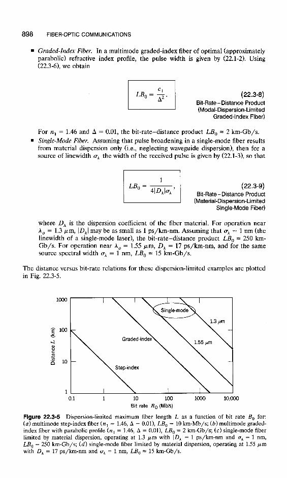
The distance versus bit-rate relations for these dispersion-limited examples are plotted in Fig. 22.3-5.
1 0.1 1 10 100 1000 10,ooo
Bit rate I30 (Mb/s)
Figure 22.3-5 Dispersion-limited maximum fiber length L as a function of bit rate Be for: (a) multimode step-index fiber (n, = 1.46, A = O.Ol>, LB, = 10 km-Mb/s; (b) multimode graded- index fiber with parabolic profile (nr = 1.46, A = O.Ol>, LB, = 2 km-Gb/s; (c) single-mode fiber limited by material dispersion, operating at 1.3 pm with ID,1 = 1 ps/km-nm and a, = 1 nm, J-0 = 250 km-Gb/s; (d) single-mode fiber limited by material with D, = 17 ps/km-nm and aA = 1 nm, LB, = 15 km-Gb/s.
dispersion, operating at 1.55 pm
SYSTEM PERFORMANCE 899
- Single-mode
1 10 100
Bit rate& (Mb/s)
1000 10,ooo
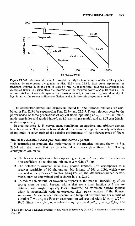
Figure 22.3-6 Maximum distance L versus bit rate Be for four examples of fibers. This graph is obtained by superposing the graphs in Figs. 22.3-4 and 22.3-5. Each curve represents the maximum distance L of the link at each bit rate Be that satisfies both the attenuation and dispersion limits, i.e., guarantees the reception of the required power and pulse width at the receiver. At low bit rates, the system is attenuation limited; L drops with B, logarithmically. At high bit rates, the system is dispersion limited and L is inversely proportional to B,.
The attenuation-limited and dispersion-limited bit-rate-distance relations are com- bined in Fig. 22.3-6 by superposing Figs. 22.3-4 and 22.3-5. These relations describe the performance of three generations of optical fibers operating at A, = 0.87 pm (multi- mode step-index and graded-index), at 1.3 pm (single-mode), and at 1.55 pm (single- mode), respectively.
In creating these L-B, curves, many simplifying assumptions and arbitrary choices have been made. The values obtained should therefore be regarded as only indications of the order of magnitude of the relative performance of the different types of fibers.
The Best Possible Fiber-Optic Communication System It is instructive to compare the performance of the practical systems shown in Fig. 22.3-7 with the “best” that can be achieved with silica glass fibers. The following assumptions are made:
. The fiber is a single-mode fiber operating at A, = 1.55 pm, where the attenua- tion coefficient is the absolute minimum ~1 = 0.16 dB/km.
. The detector is assumed ideal (i.e., photon limited). This corresponds to a receiver sensitivity of 10 photons per bit, instead of 300 or 1000, which were assumed in the previous examples. Using (22.3-5) the attenuation-limited perfor- mance may be determined and is shown in Fig. 22.3-7.
9 To reduce the material or waveguide dispersion, the spectral linewidth a,, of the source must be small. Spectral widths that are a small fraction of 1 nm are obtained with single-frequency lasers. However, an extremely narrow spectral width is incompatible with an extremely short pulse because of the Fourier transform relation between the spectral and temporal distributions. For a pulse of duration T = l/B, the Fourier-transform limited spectral width is+ a, = 1/2T = B,/2. Since v = c,/A,, a, is related to aA by aV = Idv/Jh,la, = (c,/h~)~~. The
‘This is the power-equivalent spectral width, which is defined by (A.2-10) in Appendix A and satisfies (A.2-12).
900 FIBER-OPTIC COMMUNICATIONS
0.1 1 10 100 1000 10,ooo
Bit rate B. (Mb/s)
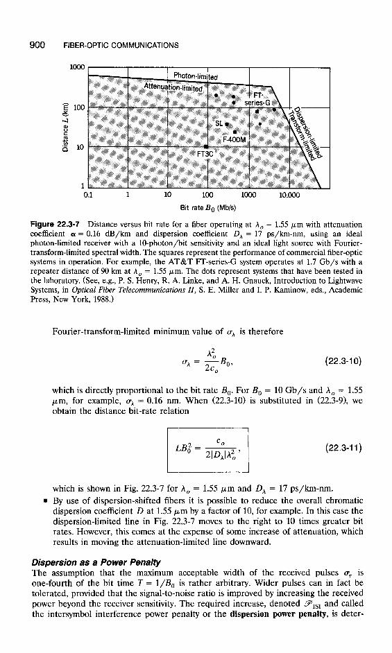
Figure 22.3-7 Distance versus bit rate for a fiber operating at A, = 1.55 pm with attenuation coefficient <y = 0.16 dB/km and dispersion coefficient D, = 17 ps/km-nm, using an ideal photon-limited receiver with a lo-photon/bit sensitivity and an ideal light source with Fourier- transform-limited spectral width. The squares represent the performance of commercial fiber-optic systems in operation. For example, the AT&T FT-series-G system operates at 1.7 Gb/s with a repeater distance of 90 km at A, = 1.55 pm. The dots represent systems that have been tested in the laboratory. (See, e.g., P. S. Henry, R. A. Linke, and A. H. Gnauck, Introduction to Lightwave Systems, in Optical Fiber Telecommunications II, S. E. Miller and I. P. Kaminow, eds., Academic Press, New York, 1988.)
Fourier-transform-limited minimum value of a,, is therefore
(22.3-10)
which is directly proportional to the bit rate B,. For B, = 10 Gb/s and A, = 1.55 pm, for example, o;\ = 0.16 nm. When (22.3-10) is substituted in (22.3-9), we obtain the distance bit-rate relation
C* LB; = - 21&b: ’
(22.3-l 1)
which is shown in Fig. 22.3-7 for A, = 1.55 pm and D, = 17 ps/km-nm. n By use of dispersion-shifted fibers it is possible to reduce the overall chromatic
dispersion coefficient D at 1.55 pm by a factor of 10, for example. In this case the dispersion-limited line in Fig. 22.3-7 moves to the right to 10 times greater bit rates. However, this comes at the expense of some increase of attenuation, which results in moving the attenuation-limited line downward.
Dispersion as a Power Penalty The assumption that the maximum acceptable width of the received pulses c7 is one-fourth of the bit time T = l/B, is rather arbitrary. Wider pulses can in fact be tolerated, provided that the signal-to-noise ratio is improved by increasing the received power beyond the receiver sensitivity. The required increase, denoted 9tsI and called the intersymbol interference power penalty or the dispersion power penalty, is deter-
0
-10 ?z g -20
t 3 B -30
jj -40
Lo
-60
-70
SYSTEM PERFORMANCE 901
A -' .-‘T
0.1 1 10 102 103 104
Bit rate (Mb/s)
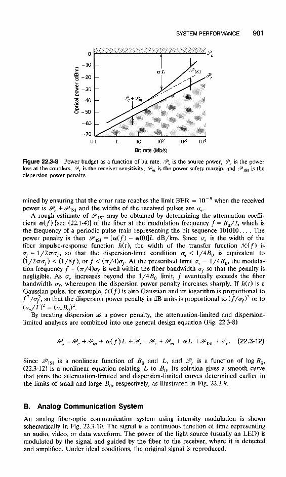
Figure 22.3-8 Power budget as a function of bit rate. gS is the source power, PC is the power loss at the couplers, ~9~ is the receiver sensitivity, 9’m is the power safety margin, and pIsI is the dispersion power penalty.
mined by ensuring that the error rate reaches the limit BER = 10d9 when the received power is Pr + Ptsl and the widths of the received pulses are a,.
A rough estimate of grsr may be obtained by determining the attenuation coeffi- cient a(f) [see (22.1-4)] of the fiber at the modulation frequency f = B,/2, which is the frequency of a periodic pulse train representing the bit sequence 101010. . . . The power penalty is then Prsl = [a(f) - ar(O)]L dB/km. Since a7 is the width of the fiber impulse-response function h(t), the width of the transfer function X(f) is Uf = 1/2TU,, so that the dispersion-limit condition a7 < l/4& is equivalent to (1/2rrof) < (l/Sf), or f < (7r/4)af. At the prescribed limit a, = l/4&, the modula- tion frequency f = (r/4) uf is well within the fiber bandwidth uf so that the penalty is negligible. As u7 increases beyond the 1/4B, limit, f eventually exceeds the fiber bandwidth af, whereupon the dispersion power penalty increases sharply. If h(t) is a Gaussian pulse, for example, X(f) is also Gaussian and its logarithm is proportional to f 2/af2T so that the dispersion power penalty in dB units is proportional to ( f/uf)2 or to (uJT>~ = b&J2.
By treating dispersion as a power penalty, the attenuation-limited and dispersion- limited analyses are combined into one general design equation (Fig. 22.3-8)
cq =LF~ +Y,,, + a( f)L +Pr =Pc +Ym + aL +gIsI +9$. (22.342)
Since PIsI is a nonlinear function of B, and L, and 9,. is a function of log B,, (22.3-12) is a nonlinear equation relating L to B,. Its solution gives a smooth curve that joins the attenuation-limited and dispersion-limited curves determined earlier in the limits of small and large B,, respectively, as illustrated in Fig. 22.3-9.
B. Analog Communication System
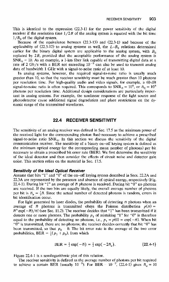
An analog fiber-optic communication system using intensity modulation is shown schematically in Fig. 22.3-10. The signal is a continuous function of time representing an audio, video, or data waveform. The power of the light source (usually an LED) is modulated by the signal and guided by the fiber to the receiver, where it is detected and amplified. Under ideal conditions, the original signal is reproduced.
902 FIBER-OPTIC ( ZOMMUNICATIONS
Attenuation-limited b.
I. ,_ ,. ,. 1. ‘, .1,, I
Bit rate B. (Mb/s)
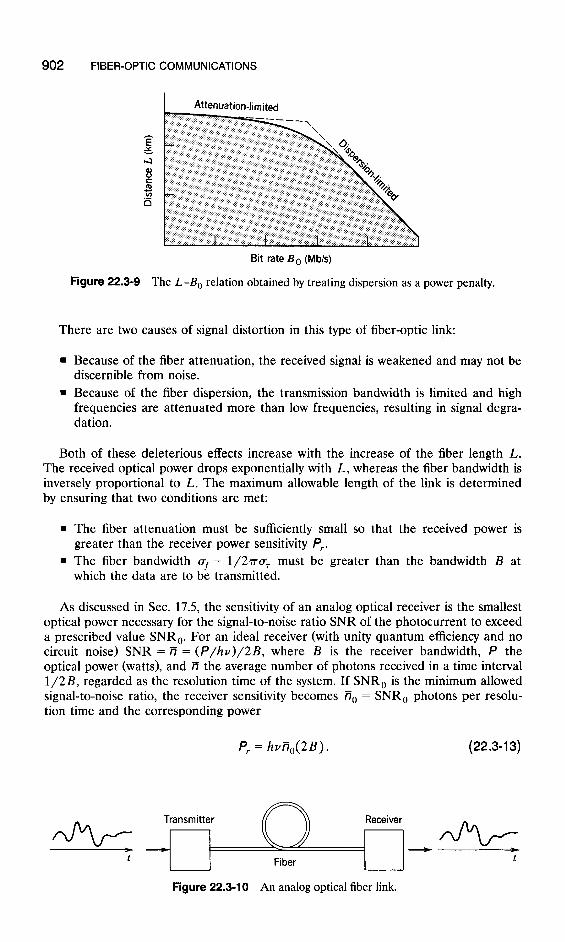
Figure 22.3-9 The L-B, relation obtained by treating dispersion as a power penalty.
There are two causes of signal distortion in this type of fiber-optic link:
n Because of the fiber attenuation, the received signal is weakened and may not be discernible from noise.
9 Because of the fiber dispersion, the transmission bandwidth is limited and high frequencies are attenuated more than low frequencies, resulting in signal degra- dation.
Both of these deleterious effects increase with the increase of the fiber length L. The received optical power drops exponentially with L, whereas the fiber bandwidth is inversely proportional to L. The maximum allowable length of the link is determined by ensuring that two conditions are met:
9 The fiber attenuation must be sufficiently small so that the received power is greater than the receiver power sensitivity P,.
. The fiber bandwidth C~ = 1/27rcr, must be greater than the bandwidth B at which the data are to be transmitted.
As discussed in Sec. 17.5, the sensitivity of an analog optical receiver is the smallest optical power necessary for the signal-to-noise ratio SNR of the photocurrent to exceed a prescribed value SNR,. For an ideal receiver (with unity quantum efficiency and no circuit noise) SNR = ii = (P/hv)/2B, where B is the receiver bandwidth, P the optical power (watts), and R the average number of photons received in a time interval 1/2B, regarded as the resolution time of the system. If SNR, is the minimum allowed signal-to-noise ratio, the receiver sensitivity becomes R, = SNR, photons per resolu- tion time and the corresponding power
P, = hvii,(2B). (22.343)
Figure 22.3-10 An analog optical fiber link.
RECEIVER SENSITIVITY 903
This is identical to the expression (22.3-1) for the power sensitivity of the digital receiver if the resolution time 1/2B of the analog system is equated with the bit time l/B, of the digital system.
Because of the equivalence between (22.3-13) and (22.3-l) and because of the applicability of (22.3-12) to analog systems as well, the L-B, relations determined earlier for the binary digital system are applicable to the analog system, with B, replaced by 2B, provided that the acceptable performance of the analog system is SNR, = 10. As an example, a l-km fiber link capable of transmitting digital data at a rate of 2 Gb/s with a BER not exceeding 10e9 can also be used to transmit analog data of bandwidth 1 GHz with a signal-to-noise ratio of at least 10.
In analog systems, however, the required signal-to-noise ratio is usually much greater than 10, so that the receiver sensitivity must be much greater than 10 photons per resolution time. For high-quality audio and video signals, for example, a 60-dB signal-to-noise ratio is often required. This corresponds to SNR,, = 106, or A, = lo6 photons per resolution time. Additional design considerations are particularly impor- tant in analog systems. For example, the nonlinear response of the light source and photodetector cause additional signal degradation and place restrictions on the dy- namic range of the transmitted waveforms.
22.4 RECEIVER SENSITIVITY
The sensitivity of an analog receiver was defined in Sec. 17.5 as the minimum power of the received light (or the corresponding photon Aux) necessary to achieve a prescribed signal-to-noise ratio SNR,. In this section we discuss the sensitivity of the digital communication receiver. The sensitivity of a binary on-off keying system is defined as the minimum optical energy (or the corresponding mean number of photons) per bit necessary to obtain a prescribed bit error rate (BER). We first determine the sensitivity of the ideal detector and then consider the effects of circuit noise and detector gain noise. This section relies on the material in Sec. 17.5.
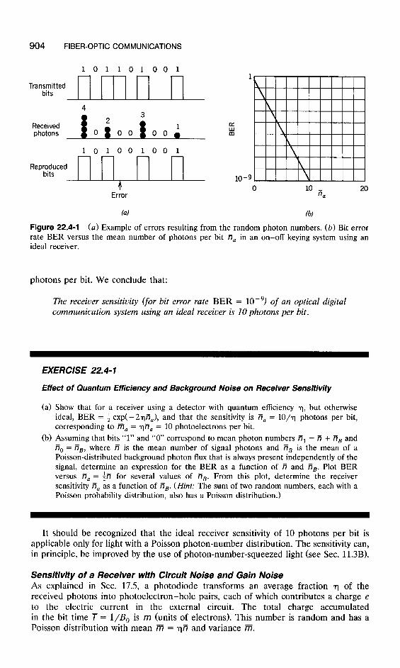
Sensitivity of the Ideal Optical Receiver Assume that bits “1” and “0” of the on-off keying system described in Sets. 22.2A and 22.3A are represented by the presence and absence of optical energy, respectively (Fig. 22.4-1). During bit “1” an average of ii photons is received. During bit “0” no photons are received. If the two bits are equally likely, the overall average number of photons per bit is n, = ifi. Since the actual number of detected photons is random, errors in bit identification occur.
For light generated by laser diodes, the probability of detecting n photons when an average of W photons is transmitted obeys the Poisson distribution p(n) = A” exp( -$/n! (see Sec. 11.2). The receiver decides that “1” has been transmitted if it detects one or more photons. The probability p1 of mistaking “1” for “0” is therefore equal to the probability of detecting no photons, i.e., pi = p(O) = exp( -iV>. When bit “0” is transmitted, there are no photons; the receiver decides correctly that bit “0” has been transmitted, so that p. = 0. The bit error rate is the average of the two error probabilities, BER = i<p, + po), from which
BER = i exp( --ii) = $ exp( -2A,). (22.4-l)
Figure 22.4-l is a semilogarithmic plot of this relation. The receiver sensitivity is defined as the average number of photons per bit required
to achieve a certain BER (usually 10p9). For BER = 10e9, (22.4-l) gives ii, = 10
904 FIBER-OPTIC COMMUNICATIONS
101101001
Tram-$ted n m n fl
4
Received photons
101001001
Rep;f;ced n n ~ n n
Error 10 n
a
(a) (bl
Figure 22.4-l (a) Example of errors resulting from the random photon numbers. (b) Bit error rate BER versus the mean number of photons per bit A, in an on-off keying system using an ideal receiver.
photons per bit. We conclude that:
The receiver sensitivity (for bit error rate BER = 10m9) of an optical digital communication system using an ideal receiver is 10 photons per bit.
EXERCISE 22.4-I
Effect of Quantum Efficiency and Background Noise on Receiver Sensitivity
(a) Show that for a receiver using a detector with quantum efficiency q, but otherwise ideal, BER = i exp( -2@J, and that the sensitivity is R, = 10/q photons per bit, corresponding to m, = $7, = 10 photoelectrons per bit.
(b) Assuming that bits “1” and “0” correspond to mean photon numbers nI = Ts + A, and ii0 = nB, where fi is the mean number of signal photons and R, is the mean of a Poisson-distributed background photon flux that is always present independently of the signal, determine an expression for the BER as a function of A and A,. Plot BER versus ii, = +H for several values of TT,. From this plot, determine the receiver sensitivity A, as a function of R,. (Hint: The sum of two random numbers, each with a Poisson probability distribution, also has a Poisson distribution.)
It should be recognized that the ideal receiver sensitivity of 10 photons per bit is applicable only for light with a Poisson photon-number distribution. The sensitivity can, in principle, be improved by the use of photon-number-squeezed light (see Sec. 11.3B).
Sensitivity of a Receiver with Circuit Noise and Gain Noise As explained in Sec. 17.5, a photodiode transforms an average fraction q of the received photons into photoelectron-hole pairs, each of which contributes a charge e to the electric current in the external circuit. The total charge accumulated in the bit time T = l/B, is m (units of electrons). This number is random and has a Poisson distribution with mean iii = TR and variance iii.
RECEIVER SENSITIVITY 905
Additional noise is introduced by the photodiode circuit in the form of a random electric current i, of Gaussian probability distribution with zero mean and variance ur2. Within the bit time interval T = l/B,, the accumulated charge q = i,T/e (in units of electrons) has an rms value gq = u,T/e. The parameter aq, called the circuit-noise parameter, depends on the receiver bandwidth B as described in Sec. 17.X.
The total accumulated charge per bit s = m + q (units of electrons) is the sum of a Poisson random variable m and an independent Gaussian random variable q. Its mean is
p=m=$q (22.4-2)
and its variance is the sum of the variances,
u2 = m + u;. (22.4-3)
When m is large, the overall distribution may be approximated by a Gaussian distribution with mean p and variance c2. We adopt this approximation in the present analysis.
For an avalanche photodiode (APD) of gain G, the mean number of photoelectrons is amplified by a factor G, but additional noise is introduced in the amplification process. The mean of the total collected charge per bit s (units of electrons)is
p=iiic (22.4-4)
and the variance is
u2 = i7iG2F + o;, (22.4-5)
where F = (G2)/( G)2 * is the excess-noise factor of the APD (see Sec. 17SB). The receiver measures the charge s accumulated in each bit (by use of an integrator,
for example) and compares it to a prescribed threshold 6. If s > 6, bit “1” is selected; otherwise, bit “0” is selected. The probabilities of error p1 and p. are determined by examining two Gaussian probability distributions of s that have
mean p. = 0, variance U: = 6~: for bit “0”
(22.4-6) mean pl = ii%?, variance a: = i7iG2F + o-t for bit “1.”
The probability p. of mistaking “0” for “1” is the integral of a Gaussian probability distribution p(s) with mean p. and variance 0: from s = 6 to s = ~0. The probability p1 of mistaking “1” for “0” is the integral of a Gaussian probability distribution with mean pl and variance 2 u1 from s = -a~ to s = 6. The threshold 6 is selected such that the average probability of error BER = i(po + pl) is minimized.
This type of analysis is the basis of the conventional theory of binary detection in the presence of Gaussian noise. If p. and pl, and U; and uf are the means and variances associated with two Gaussian variables representing bits “0” and “1,” and if a0 and u1 are much smaller than ,~i - po, the bit error rate for an optimal-threshold receiver is approximately
BER=$[l-erf(-$)], (22.4-7)
906 FIBER-OPTIC COMMUNICATIONS
where
PI - PO Q=---
go + u1
and
erf( 2) = $i’exp( -x2) &
(22.4-8)
(22.4-9)
is the error function. When Q = 6, BER = lo-“. The receiver sensitivity therefore corresponds to Q = 6, or
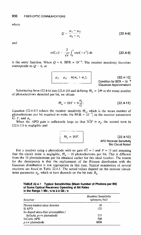
Substituting from (22.4-6) into (22.4-10) and defining m, = $7 as the mean number of photoelectrons detected per bit, we obtain
(22.4-l 1)
Equation (22.4-11) relates the receiver sensitivity i7i,, which is the mean number of photoelectrons per bit required to make the BER = 10m9, to the receiver parameters G, F, and ua.
When the APD gain is sufficiently large so that 3GF >> as, the second term in (22.4-11) is negligible and
/ m,=18F. 1 (22.4-12) APD Receiver Sensitivity
(No Circuit Noise)
For a receiver using a photodiode with no gain (c = 1 and F = 1) and assuming that the circuit noise is negligible, m, = 18 photoelectrons per bit. This is different from the 10 photoelectrons per bit obtained earlier for this ideal receiver. The reason for the discrepancy is that the replacement of the Poisson distribution with the Gaussian distribution is not appropriate in this case. Typical sensitivities of several receivers are listed in Table 22.4-l. The actual values depend on the receiver circuit- noise parameter aq, which in turn depends on the bit rate B,.
TABLE 22.4-l Typical Sensitivities (Mean Number of Photons per Bit) of Some Optical Receivers Operating at Bit Rates in the Range 1 Mb/s to 2.5 Gb/s
Receiver Receiver Sensitivity
(photons/bit)
Photon-limited ideal detector Si APD Er-doped silica-fiber preamplifier/
InGaAs p-i-n photodiode InGaAs APD p-i-n photodiode
10 125
215 500
6000
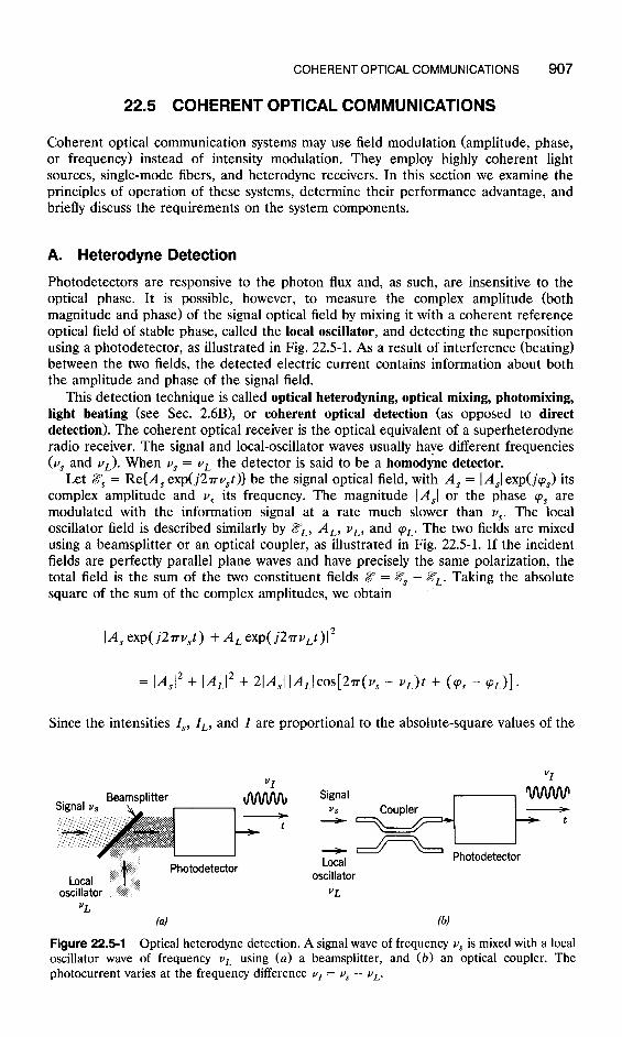
COHERENT OPTICAL COMMUNICATIONS 907
22.5 COHERENT OPTICAL COMMUNICATIONS
Coherent optical communication systems may use field modulation (amplitude, phase, or frequency) instead of intensity modulation. They employ highly coherent light sources, single-mode fibers, and heterodyne receivers. In this section we examine the principles of operation of these systems, determine their performance advantage, and briefly discuss the requirements on the system components.
A. Heterodyne Detection
Photodetectors are responsive to the photon flux and, as such, are insensitive to the optical phase. It is possible, however, to measure the complex amplitude (both magnitude and phase) of the signal optical field by mixing it with a coherent reference optical field of stable phase, called the local oscillator, and detecting the superposition using a photodetector, as illustrated in Fig. 22.5-l. As a result of interference (beating) between the two fields, the detected electric current contains information about both the amplitude and phase of the signal field.
This detection technique is called optical heterodyning, optical mixing, photomixing, light beating (see Sec. 2.6B), or coherent optical detection (as opposed to direct detection). The coherent optical receiver is the optical equivalent of a superheterodyne radio receiver. The signal and local-oscillator waves usually have different frequencies (v, and vL). When us = vL the detector is said to be a homodine detector.
Let &Ys = Re{A, exp(j2rv,t)} be the signal optical field, with A, = 1 A,[ exp(j9,) its complex amplitude and v, its frequency. The magnitude IA,1 or the phase ‘ps are modulated with the information signal at a rate much slower than vs. The local oscillator field is described similarly by gL, A,, v~, and (pL. The two fields are mixed using a beamsplitter or an optical coupler, as illustrated in Fig. 22.5-l. If the incident fields are perfectly parallel plane waves and have precisely the same polarization, the total field is the sum of the two constituent fields Z = &Ys + gL. Taking the absolute square of the sum of the complex amplitudes, we obtain
1 A, exp( j2rrv,t) + A, exp( j2rvLt)12
= IAs12 + IALl + 441 lALb[2+, - v& + (9, - cp,)].
Since the intensities I,, IL, and I are proportional to the absolute-square values of the
f Photodetector
Local oscillator
Signal vs
LoCa I oscillator
VL
If frequency vS is mixed with a local and (b) an optical coupler. The
Figure 22.5-l Optical heterodyne detection. A signal wave o oscillator wave of frequency vL using (a) a beamsplitter, photocurrent varies at the frequency difference vl = vS - vL.
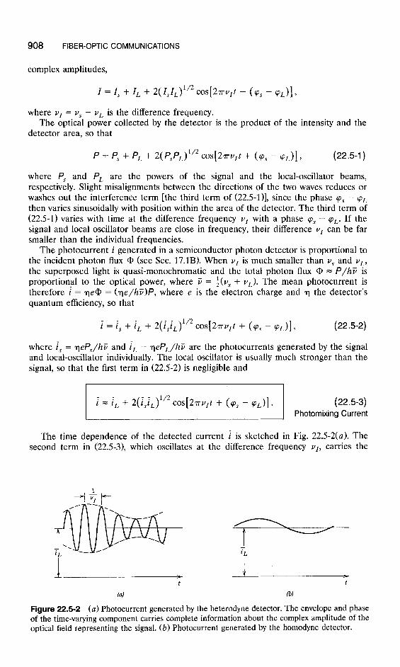
908 FIBER-OPTIC COMMUNICATIONS
complex amplitudes,
I = I, + IL + 2( I&y2 cos[27yt + ( cps - cp,)] )
where vI = vs - vL is the difference frequency. The optical power collected by the detector is the product of the intensity and the
detector area, so that
P = Ps + PL + 2(PsPL)"2cos[2av,t + (cp, - cp,)], (22.5-l)
where P, and PL are the powers of the signal and the local-oscillator beams, respectively. Slight misalignments between the directions of the two waves reduces or washes out the interference term [the third term of (22.5-l)], since the phase cps - (pL then varies sinusoidally with position within the area of the detector. The third term of (22.5-l) varies with time at the difference frequency v1 with a phase ‘ps - <pL. If the signal and local oscillator beams are close in frequency, their difference vI can be far smaller than the individual frequencies.
The photocurrent i generated in a semiconductor photon detector is proportional to the incident photon flux @ (see Sec. 17.1B). When vI is much smaller than v, and vL, the superposed light is quasi-monochromatic and the total photon flux CD = P/hF is proportional to the optical power, where V = +(v~ + vL). The mean photocurrent is therefore i = TeCD = (qe/hF)P, where e is the electron charge and q the detector’s quantum efficiency, so that
E = i, + E, + 2(t,ELy2 cospyt + bs - qL)l?
where E, = qeP,/hF and EL = qeP,/h- v are the photocurrents generated by the signal and local-oscillator individually. The local oscillator is usually much stronger than the signal, so that the first term in (22.5-2) is negligible and
i z iL + 2(IslLy2 c427w + (cp, - cpL>l* (22.5-3) Photomixing Current
The time dependence of the detected current E is sketched in Fig. 22.5-2(a). The second term in (22.5-3), which oscillates at the difference frequency vi, carries the
A- / J b t t
(al lb)
Figure 22.5-2 (a) Photocurrent generated by the heterodyne detector. The envelope and phase of the time-varying component carries complete information about the complex amplitude of the optical field representing the signal. (b) Photocurrent generated by the homodyne detector.
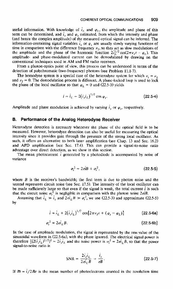
COHERENT OPTICAL COMMUNICATIONS 909
useful information. With knowledge of t, and (pL, the amplitude and phase of this term can be determined, and E, and ‘ps estimated, from which the intensity and phase (and hence the complex amplitude) of the measured optical signal can be inferred. The information-containing signal variables E, or ‘ps are usually slowly varying functions of time in comparison with the difference frequency vi, so they act as slow modulations of the amplitude and the phase of the harmonic function 2iz/” cos(27rv,t - pL). This amplitude- and phase-modulated current can be demodulated by drawing on the conventional techniques used in AM and FM radio receivers.
From a photon-optics point of view, this process can be understood in terms of the detection of polychromatic (two-frequency) photons (see Problem 11.1-7).
The homodyne system is a special case of the heterodyne system for which vs = vL and vI = 0. The demodulation process is different. A phase-locked loop is used to lock the phase of the local oscillator so that (pL = 0 and (22.5-3) yields
E = EL + 2( EsELy2 cos ‘ps. (22.54)
Amplitude and phase modulation is achieved by varying i, or q,, respectively.
B. Performance of the Analog Heterodyne Receiver
Heterodyne detection is necessary whenever the phase of the optical field is to be measured. However, heterodyne detection can also be useful for measuring the optical intensity since it provides gain through the presence of the strong local oscillator. As such, it offers an alternative to both laser amplification (see Chap. 13 and Sec. 16.2) and APD amplification (see Sec. 17.4). This can provide a signal-to-noise ratio advantage over direct detection, as we show in this section.
The mean photocurrent E generated by a photodiode is accompanied by noise of variance
u.~ = 2eiB + a2 1 r 7 (22.5-5)
where B is the receiver’s bandwidth; the first term is due to photon noise and the second represents circuit noise (see Sec. 17.5). The intensity of the local oscillator can be made sufficiently large so that even if the signal is weak, the total current i is such that the circuit noise u: is negligible in comparison with the photon noise 2eiB.
Assuming that EL B E, and 2eE,B za or2, we use (22.5-3) and approximate (22.55) by
: z=z TL + 2(IslLy2 co+w + (cp, - cpL>l (22.5-6a)
q2 z 2ei, B. (22.5-6b)
In the case of amplitude modulation, the signal is represented by the rms value of the sinusoidal waveform in (22.5-6a), with the phase ignored. The electrical signal power is therefore i[2(E,1L)*/2]2 = 2E,EL and the noise power is *i2 = 2ei,B, so that the power signal-to-noise ratio is
SNR = 2E,E, E,
-=- 2ei,B eB ’
(22.5-7)
If m = E/2Be is the mean number of photoelectrons counted in the resolution time
910 FIBER-OPTIC COMMUNICATIONS
interval T = 1/2B, then
In comparison, the SNR of the direct-detection photodiode same signal current i, without the benefit of heterodyning is
/ SNR=2m. / (22.58) Signal-to-Noise Ratio
of a Heterodyne Receiver
E2 in2 SNR =
s 2ei,B + “,2
=- m -I- cTq2 ’
receiver measuring the
(22.59)
where U: = (u,./2Bej2 is the circuit-noise parameter discussed in Sec. 17.X. The principal advantage of the heterodyne system is now apparent. For strong light or low circuit noise (i?? Z+ u:>, the direct-detection result is SNR = E?. The heterodyne receiver, which yields SNR = 2Ei, offers a factor-of-2 improvement (3-dB advantage). But for weak light (or large circuit noise) the advantage can be even more substantial, since the heterodyne receiver has SNR = 2m, whereas the SNR of the direct-detection receiver is reduced by circuit noise to SNR = m/(1 + ~t/m).
The performance of a direct-detection avalanche photodiode receiver is also infe- rior to that of a heterodyne photodiode receiver. In accordance with (17.5-32), the SNR obtained when the APD gain is sufficiently large to overcome circuit noise is
-
SNR = ;,
where F is the APD excess noise factor (F > 1). Therefore, even a noiseless APD receiver (F = 1) is a factor of 2 inferior to the heterodyne receiver.
Advantages of Heterodyne Receivers In comparison with the direct-detection receiver, the heterodyne receiver has the following advantages:
. It is capable of measuring the optical phase and frequency. n It permits the use of wavelength-division multiplexing (WDM) with smaller
channel spacing (= 100 MHz). In conventional direct-detection systems the channel spacing is of the order of 100 GHz.
. It permits the use of electronic equalization to compensate for pulse broadening in the fiber. Pulse broadening is a result of the dephasing of the different wavelength/frequency components because of differences in group velocities. Since the receiver monitors the phase, this dephasing may be removed by proper electronic filtering.
. By use of a strong reference field, the heterodyne receiver has an inherent noiseless gain conversion factor that effectively amplifies the signal above the circuit noise level.
n It provides a 3-dB advantage over even the noiseless direct-detection receiver. n It is insensitive to unwanted background light with which the local oscillator does
not mix. Heterodyning is one of the few ways of attaining photon-noise-limited detection in the infrared, where background noise is so prevalent.
The cost of these advantages is an increase in the system’s complexity since heterodyning requires a stable local oscillator, an optical coupler in which the mixed fields are precisely aligned, and complex circuits for phase locking.
COHERENT OPTICAL COMMUNICATIONS 911
C. Performance of the Digital Heterodyne Receiver
In this section the performance and sensitivity of a digital coherent comm system are determined in the cases of amplitude and phase modulation.
unication
On -Off Keying (OOK) Homodyne System Consider an on-off keying COOK) system transmitting data at a rate B, bits/s and using a homodyne receiver. Bits “1” and “0” are represented by the presence and absence of the signal E, during the bit time T = l/B,, respectively. Assuming that cps = 9, = 0 and vi = vs - vL = 0, the measured current has the following means and variances obtained from (22.56a) and (22.5~6b):
mean p1 = EL + 2(iLE,)1’2, variance a: = 2E,eB for bit “1” (22.510)
mean p. = EL, variance at = 2E,eB for bit “0.”
The receiver bandwidth B = B,/2 since the bit time T = l/B, is the sampling time 1/2B for a signal of bandwidth B.
The performance of the binary communication system under the Gaussian approxi- mation has been discussed in Sec. 22.4. The bit error rate is given by (22.4-7), where
l/2 Pu, - PO Q=------= = j771/2
(Tl + go , (22.511)
and m = iJ2eB is the mean number of detected photoelectrons in bit 1. For a bit error rate BER = 10T9, Q = 6 and therefore m = 36, corresponding to a receiver sensitivity m, = $m = 18 photoelectrons per bit (averaged over both bits).
Phase-Shift-Keying (PSK) Homodyne System Here bits “1” and “0” are represented by a phase shift cps = 0 and 7~, respectively. Assuming that cp - 0, the means and variances of the photocurrent for bits “1” and “0” are , from (22L56) *- ,
mean p1 = EL + 2(iLis)1’2, variance a: = 2eEL B for bit “1”
mean p. = EL - 2(iLE,)1’2, variance 0: = 2ei,B for bit “0”
and therefore
l/2 Pl - PO
Q=------
01 + a0
= 2(m)“2. (22.512)
For a BER = 10M9, Q = 6, from which iiV = 9. Since each of the two bits must carry an average of nine photoelectrons in this case, the average number of photoelectrons per bit is i??, = m = 9. It follows that the receiver sensitivity is 9 photoelectrons/bit. The PSK homodyne receiver is twice as sensitive as the OOK homodyne receiver because it requires half the number of photoelectrons.
Comparison The sensitivity of the heterodyne digital receiver can be determined by following a similar analysis. Table 22.51 lists the receiver sensitivities of several digital modulation systems, assuming q = 1. Although it appears that the direct-detection OOK system has about the same performance as the best coherent system (homodyne PSK), in
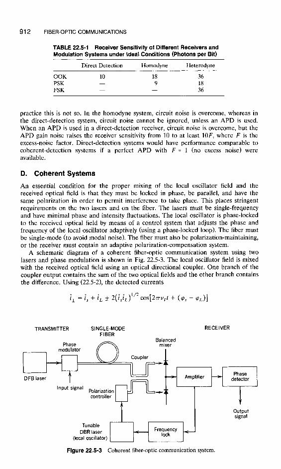
912 FIBER-OPTIC COMMUNICATIONS
TABLE 22.5-l Receiver Sensitivity of Different Receivers and Modulation Systems under Ideal Conditions (Photons per Bit)
Direct Detection Homodyne Heterodyne
OOK 10 18 36 PSK - 9 18 FSK - - 36
practice this is not so. In the homodyne system, circuit noise is overcome, whereas in the direct-detection system, circuit noise cannot be ignored, unless an APD is used. When an APD is used in a direct-detection receiver, circuit noise is overcome, but the APD gain noise raises the receiver sensitivity from 10 to at least lOF, where F is the excess-noise factor. Direct-detection systems would have performance comparable to coherent-detection systems if a perfect APD with F = 1 (no excess noise) were available.
D. Coherent Systems
An essential condition for the proper mixing of the local oscillator field and the received optical field is that they must be locked in phase, be parallel, and have the same polarization in order to permit interference to take place. This places stringent requirements on the two lasers and on the fiber. The lasers must be single-frequency and have minimal phase and intensity fluctuations. The local oscillator is phase-locked to the received optical field by means of a control system that adjusts the phase and frequency of the local oscillator adaptively (using a phase-locked loop). The fiber must be single-mode (to avoid modal noise). The fiber must also be polarization-maintaining, or the receiver must contain an adaptive polarization-compensation system.
A schematic diagram of a coherent fiber-optic communication system using two lasers and phase modulation is shown in Fig. 22.53. The local oscillator field is mixed with the received optical field using an optical directional coupler. One branch of the coupler output contains the sum of the two optical fields and the other branch contains the difference. Using (22.52), the detected currents
: l* = E, + iL f 2( ISlJ’2 427w + (cp, - cp,,]
TRANSMITTER SINGLE-MODE RECEIVER FIBER
Balanced mixer
DFB laser Phase
tcf Amplifier * detector
controller
Tunable DBR laser
(local oscillator)
Y
output signal
Figure 22.5-3 Coherent fiber-optic communication system.
READING LIST 913
are subtracted electronically, yielding 4(E,1,)1/2 cos[27rv1t + (cp, - qL)], which is de- modulated to recover the message. This type of coherent receiver is known as a balanced mixer. It has the advantage of canceling out intensity fluctuations of the local oscillator. A number of coherent fiber-optic communication systems have been imple- mented at A, = 1.55 pm (where fiber attenuation is minimal) with bit-rate-distance products matching theoretical expectations.
One example is provided by a system operating at a bit rate = 4 Gb/s. A DFB laser with a 15-MHz CW linewidth was directly modulated in an FSK signal format. The local oscillator was a tunable DBR laser (see Sec. 16.3E). This system exhibited a receiver sensitivity = 190 photons/bit and was used for transmission over a 160~km length of fiber.
READING LIST
See also the reading lists in Chapters 7, 8, 16, 17, and 21.
Books T. Li, ed., Optical Fiber Data Transmission, Academic Press, Boston, 1991. H. B. Killen, Fiber Optic Communications, Prentice Hall, Englewood Cliffs, NJ, 1991. P. K. Cheo, Fiber Optics and Optoelectronics, Prentice Hall, Englewood Cliffs, NJ, 1990. T. C. Edwards, Fiber-Optic Systems: Network Applications, Wiley, New York, 1989. J. C. A. Chaimowicz, Lightwave Technology, Butterworths, Boston, 1989. C. Lin, ed., Optoelectronic Technology and Lightwave Communications Systems, Van Nostrand
Reinhold, New York, 1989. S. E. Miller and I. P. Kaminow, eds., Optical Fiber Telecommunications II, Academic Press, New
York, 1988. S. Karp, R. Gagliardi, S. E. Moran, and A. Holland, Optical Channels: Fibers, Clouds, Water, and
the Atmosphere, Plenum Press, New York, 1988. W. B. Jones, Jr., Introduction to Optical Fiber Communication Systems, Holt, Rinehart and
Winston, New York, 1988. J. C. Palais, Fiber Optic Communications, Prentice Hall, Englewood Cliffs, NJ, 2nd ed. 1988. T. Okoshi and K. Kikuchi, Coherent Optical Fiber Communications, Kluwer, Boston, 1988. C. K. Kao, Optical Fibre, Peter Peregrinus, London, 1988. C. D. Chaffee, The Rewiring of America: The Fiber Optics Revolution, Academic Press, Boston,
1988. H. F. Taylor, ed., Advances in Fiber Optics Communications, Artech House, Nor-wood, MA, 1988. S. Geckeler, Optical Fiber Transmission Systems, Artech House, Norwood, MA, 1987. G. Mahlke and P. G&sing, Fiber Optic Cables, Wiley, New York, 1987. P. K. Runge and P. R. Trischitta, eds., Undersea Lightwave Communications, IEEE Press, New
York, 1986. C. Baack, ed., Optical Wideband Transmission Systems, CRC Press, Boca Raton, FL, 1986. S. D. Personick, Fiber Optics: Technology and Applications, Plenum Press, New York, 1985. D. G. Baker, Fiber Optic Design and Applications, Reston Publishing, Reston, VA, 1985. J. M. Senior, Optical Fiber Communications, Prentice-Hall, Englewood Cliffs, NJ, 1985. J. Gowar, Optical Communication Systems, Prentice-Hall, Englewood Cliffs, NJ, 1984. B. Culshaw, Optical Fibre Sensing and Signal Processing, Peter Peregrinus, London, 1984. J. C. Daly, ed., Fiber Optics, CRC Press, Boca Raton, FL, 1984. A. H. Cherin, An Introduction to Optical Fibers, McGraw-Hill, New York, 1983. G. Keiser, Optical Fiber Communications, McGraw-Hill, New York, 1983.
914 FIBER-OPTIC COMMUNICATIONS
D. J. Morris, Pulse Code Formats for Fiber Optical Data Communication: Basic Principles and Applications, Marcel Dekker, New York, 1983.
H. F. Taylor, ed., Fiber Optics Communications, Artech House, Dedham, MA, 1983. Y. Suematsu and K. Iga, Introduction to Optical Fiber Communications, Wiley, New York, 1982. H. Kressel, ed., Semiconductor Devices for Optical Communication, Springer-Verlag, New York,
2nd ed. 1982. T. Okoshi, Optical Fibers, Academic Press, New York, 1982. C. K. Kao, Optical Fiber Systems, McGraw-Hill, New York, 1982. S. D. Personick, Optical Fiber Transmission Systems, Plenum Press, New York, 1981. M. K. Barnoski, ed., Fundamentals of Optical Fiber Communications, Academic Press, New York,
2nd ed. 1981. A. B. Sharma, S. J. Halme, and M. M. Butusov, Optical Fiber Systems and Their Components,
Springer-Verlag, Berlin, 1981. CSELT (Centro Studi e Laboratori Telecomunicazioni), Optical Fibre Communications,
McGraw-Hill, New York, 1981. C. P. Sandbank, ed., Optical Fibre Communication Systems, Wiley, New York, 1980. M. J. Howes and D. V. Morgan, eds., Optical Fibre Communications, Wiley, New York, 1980. J. E. Midwinter, Optical Fibers for Transmission, Wiley, New York, 1979. S. E. Miller and A. G. Chynoweth, Optical Fiber Telecommunications, Academic Press, New York,
1979. B. Saleh, Photoelectron Statistics with Applications to Spectroscopy and Optical Communication,
Springer-Verlag, Berlin, 1978. G. R. Elion and H. A. Elion, Fiber Optics in Communication Systems, Marcel Dekker, New York,
1978. R. 0. Harger, Optical Communication Theory, Dowden, Hutchinson & Ross, Stroudsburg, PA,
1977. R. M. Gagliardi and S. Karp, Optical Communications, Wiley, New York, 1976. W. K. Pratt, Laser Communication Systems, Wiley, New York, 1969.
Special Journal Issues Special issue on optical fiber communication, Optics and Photonics News, vol. 1, no. 11, 1990. Special issue on wide-band optical transmission technology and systems, Journal of Lightwave
Technology, vol. LT-6, no. 11, 1988. Special issue on fiber optic local and metropolitan area networks, IEEE Journal of Selected Areas
in Communications, vol. SAC-6, no. 6, 1988. Special issue on factors affecting data transmission quality, Journal of Lightwave Technology, vol.
LT-6, no. 5, 1988. Special issue on high speed technology for lightwave applications, Journal of Lightwave Technol-
ogy, vol. LT-5, no. 10, 1987. Special issue on coherent communications, Journal of Lightwave Technology, vol. LT-5, no. 4,
1987. Special issue on fiber optic systems for terrestrial
Communications, vol. SAC-4, no. 9, 1986. applications, IEEE Journal of Selected Areas in
Joint special issue on lightwave devices and subsystems, Journal of Lightwave Technology, vol. LT-3, no. 6; and IEEE Transactions on Election Devices, vol. ED-32, no. 12, 1985.
Special issue on fiber optics for local communications, IEEE Journal of Selected Areas in Communications, vol. SAC-3, no. 6, 1985.
Joint special issue on undersea lightwave communications, Journal of Lightwave Technology, vol. LT-2, no. 6; and IEEE Journal of Selected Areas in Communications, vol. SAC-2, no. 6, 1984.
Special issue on fiber optic systems, IEEE Journal of Selected Areas in Communications, vol. SAC-l, no. 3, 1983.
integrated optical Special issue on communications aspects of single-mode optical fiber technology, IEEE Journal of Quantum Electronics, vol. QE-17, no. 6,
and 1981.
PROBLEMS 915
Special issue on optical-fiber communications, Proceedings of the IEEE, vol. 68, no. 10, 1980. Special issue on quantum-electronic devices for optical-fiber communications, IEEE Journal of
Quantum Electronics, vol. QE-14, no. 11, 1978. Special issue on optical communication, Proceedings of the IEEE, vol. 58, no. 10, 1970.
Articles
E. Desurvire, Erbium-Doped Fiber Amplifiers for New Generations of Optical Communication Systems, Optics & Photonics News, vol. 2, no. 1, pp. 6-11, 1991.
K. Nakagawa and S. Shimada, Optical Amplifiers in Future Optical Communication Systems, IEEE Lightwave Communication Systems Magazine, vol. 1, no. 4, pp. 57-62, 1990.
P. E. Green and R. Ramaswami, Direct Detection Lightwave Systems: Why Pay More?, IEEE Lightwave Communication Systems Magazine, vol. 1, no, 4, pp. 36-49, 1990.
R. E. Wagner and R. A. Linke, Heterodyne Lightwave Systems: Moving Towards Commercial Use, IEEE Lightwave Communication Systems Magazine, vol. 1, no. 4, pp. 28-35, 1990.
J. A. Jay and E. M. Hopiavuori, Dispersion-Shifted Fiber Hits its Stride, Photonics Spectra, vol. 24, no. 9, pp. 153-158, 1990.
M. G. Drexhage and C. T. Moynihan, Infrared Optical Fibers, Scientific American, vol. 259, no. 5, pp. 110-116, 1988.
R. A. Linke and A. H. Gnauck, High-Capacity Coherent Lightwave Systems, Journal of Light- waue Technology, vol. 6, pp. 1750-1769, 1988.
S. F. Jacobs, Optical Heterodyne (Coherent) Detection, American Journal of Physics, vol. 56, pp. 235-245, 1988.
K. NOSU, Advanced Coherent Lightwave Technologies, IEEE Communications Magazine, vol. 26, no. 2, pp. 15-21, 1988.
W. J. Tomlinson and C. A. Brackett, Telecommunications Applications of Integrated Optics and Optoelectronics, Proceedings of the IEEE, vol. 75, pp. 1512-1523, 1987.
R. A. Linke and P. S. Henry, Coherent Optical Detection: A Thousand Calls on One Circuit, IEEE Spectrum, vol. 24, no. 2, pp. 52-57, 1987.
S. R. Nagel, Optical Fiber-the Expanding Medium, IEEE Communications Magazine, vol. 25, no. 4, pp. 33-43, 1987.
T. Li, Advances in Lightwave Systems Research, AT & T Technical Journal, vol. 66, no. 1, pp. 5-18, 1987.
H. Kogelnik, High-Speed Lightwave Transmission in Optical Fibers, Science, vol. 228, pp. 1043-1048, 1985.
M. C. Teich, Laser Heterodyning, Optica Acta (Journal of iModern Optics), vol. 32, pp. 1015-1021, 1985.
P. S. Henry, Lightwave Primer, IEEE Journal of Quantum EZectronics, vol. QE-21, pp. 1862-1879, 1985.
I. W. Stanley, A Tutorial Review of Techniques for Coherent Optical Fiber Transmission Systems, IEEE Communications Magazine, vol. 23, no. 8, pp. 37-53, 1985.
T. Li, Lightwave Telecommunication, Physics Today, vol. 38, no. 5, pp. 24-31, 1985. J. D. Crow, Computer Applications for Fiber Optics, IEEE Communications Magazine, vol. 23,
no. 2, pp. 16-20, 1985. Y. Suematsu, Long-Wavelength Optical Fiber Communication, Proceedings of the IEEE, vol. 71,
pp. 692-721, 1983.
PROBLEMS
22.1-1 Fiber-Optic Systems. Discuss the validity of each of the following statements and indicate the conditions under which your conclusion is applicable. (a) The wavelength A, = 1.3 pm is preferred to A, = 0.87 pm for all fiber-optic communication systems.
916
22.1-2
22.3-l
22.3-2
22.4-l
22.4-2
22.4-3
FIBER-OPTIC COMMUNICATIONS
(b) The wa ve ength 1 A, = 1.55 pm is preferred to A, = 1.3 for all fiber-optic communication systems. (c) Single-mode fibers are superior to multimode fibers because they have lower attenuation coefficients. (d) There is no pulse spreading at A, = 1.312 ,um in silica glass fibers. (e) Compound semiconductor devices are required for fiber-optic communication systems. (f) APDs are noisier than p-i-n photodiodes and are therefore not useful for fiber-optic systems.
Components for Fiber-Optic Systems. The design of a fiber-optic communication system involves many choices, some of which are shown in Table 22.1-2 on page 886. Make reasonable choices for each of the applications listed below. More than one answer may be correct. Some choices, however, are incompatible. (a) A transoceanic cable carrying data at a loo-Mb/s rate with loo-km repeater spacings. (b) A l-m cable transmitting analog data from a sensor at 1 kHz. (c) A link for a computer local-area network operating at 500 Mb/s. (d) A l-km d t 1’ k a a m operating at 100 Mb/s with +5O”C temperature variations.
Performance of a Plastic Fiber Link. A short-distance low-data-rate communica- tion system uses a plastic fiber with attenuation coefficient 0.5 dB/m, an LED generating 1 mW at a wavelength of 0.87 ,um, and a photodiode with receiver sensitivity -20 dBm. Assuming a power loss of 3 dB each at the input and output couplers, determine the maximum length of the link. Assume that the data rate is sufficiently low so that dispersion effects play no role.
Power Budget. A fiber-optic communication link is designed for operation at 10 Mb/s. The source is a 1-mW AlGaAs diode laser operating at 0.87 pm. The fiber is made of l-km segments each with attenuation 3.5 dB/km. Connectors between segments have a loss of 2 dB each and input and output couplers each introduce a loss of 2 dB. The safety margin is 6 dB. Two receivers are available, a Si p-i-n photodiode receiver with sensitivity 5000 photons per bit, and a Si APD with sensitivity 125 photons per bit. Determine the maximum length of the link for each receiver.
Dependence of Receiver Sensitivity on Wavelength. The receiver sensitivity of an ideal receiver (with unity quantum efficiency and no circuit noise) operating at a wavelength 0.87 pm is -76 dBm. What is the sensitivity at 1.3 pm if the receiver is operated at the same data rate?
Bit Error Rates. A quantum-limited p-i-n photodiode (no noise other than photon noise) of quantum efficiency q = 1 mistakes a present A, = 0.87 pm optical signal of power P (bit 1) for an absent signal (bit 0) with probability 10-r’. What is the probability of error under each of the following new conditions? (a) The wavelength is A, = 1.3 pm. (b) Original conditions, but now the power is doubled. (c) Original conditions, but the efficiency is now rl = 0.5. (d) Original conditions, but an ideal APD with q = 1 and gain G = 100 (no gain noise) is used. (e) As in part (d), but the APD has an excess noise factor F = 2 instead.
Sensitivity of an AM Receiver. A detector with responsivity ZIl (A/W), bandwidth B, and negligible circuit noise, measures a modulated optical power p(t) = PO + P, cos(2rft), with f < B. If PO X+ P,, derive an expression for the minimum modulation power P, that is measurable with signal-to-noise ratio SNR, = 30 dB. What is the effect of the background power PO on the minimum observable signal P?
PROBLEMS 917
22.4-4 Maximum Length of an Analog Link. A fiber-optic communication link uses intensity modulation to transmit data at a bandwidth B = 10 MHz and signal-to- noise ratio of 40 dB. The source is a h, = 0.87 pm light-emitting diode producing 100 PW average power with maximum modulation index of 0.5. The fiber is a multimode step-index fiber with attenuation coefficient 2.5 dB/km. The detector is an avalanche photodiode with mean gain G = 100, excess noise factor F = 5, and responsivity of 0.5 A/W (not including the gain). Assuming that the circuit noise is negligible, calculate the optical power sensitivity of the receiver and the attenua- tion-limited maximum length L of the fiber.
22.4-5 Sensitivity of a Photon-Counting Receiver. A photodetector of quantum efficiency q = 0.5 counts photoelectrons received in successive time intervals of duration T = 1 pus. Determine the receiver sensitivity (mean number of photons required to achieve SNR = 103) assuming a Poisson photon-number distribution. Assuming that the wavelength of the light is h, = 0.87 pm, what is the corresponding optical power? If this optical power is received, what is the probability that the detector registers zero counts?