Chapter 12: Portfolio Selection and Diversification

Copyright © Prentice Hall Inc. 1999. Author: Nick Bagley

ObjectiveTo understand the theory of personal

portfolio selection in theory and in practice

Chapter 12 Contents

• 12.1 The process of personal portfolio selection

• 12.2 The trade-off between expected return and risk

• 12.3 Efficient diversification with many risky assets

Objectives

• To understand the process of personal portfolio selection in theory and practice

Introduction

• How should you invest your wealth optimally?– Portfolio selection

• Your wealth portfolio contains– Stock, bonds, shares of unincorporated

businesses, houses, pension benefits, insurance policies, and all liabilities

Portfolio Selection Strategy

• There are general principles to guide you, but the implementation will depend such factors as your (and your spouse’s)– age, existing wealth, existing and target level

of education, health, future earnings potential, consumption preferences, risk preferences, life goals, your children’s educational needs, obligations to older family members, and a host of other factors

12.1 The Process of Personal Portfolio Selection

• Portfolio selection– the study of how people should invest their

wealth– process of trading off risk & expected return to

find the best portfolio of assets & liabilities• Narrower dfn: consider only securities

• Wider dfn: house purchase, insurance, debt

• Broad dfn: human capital, education

The Life Cycle

• The risk exposure you should accept depends upon your age

• Consider two investments (rho=0.2)– Security 1 has a volatility of 20% and an

expected return of 12%– Security 2 has a volatility of 8% and an

expected return of 5%

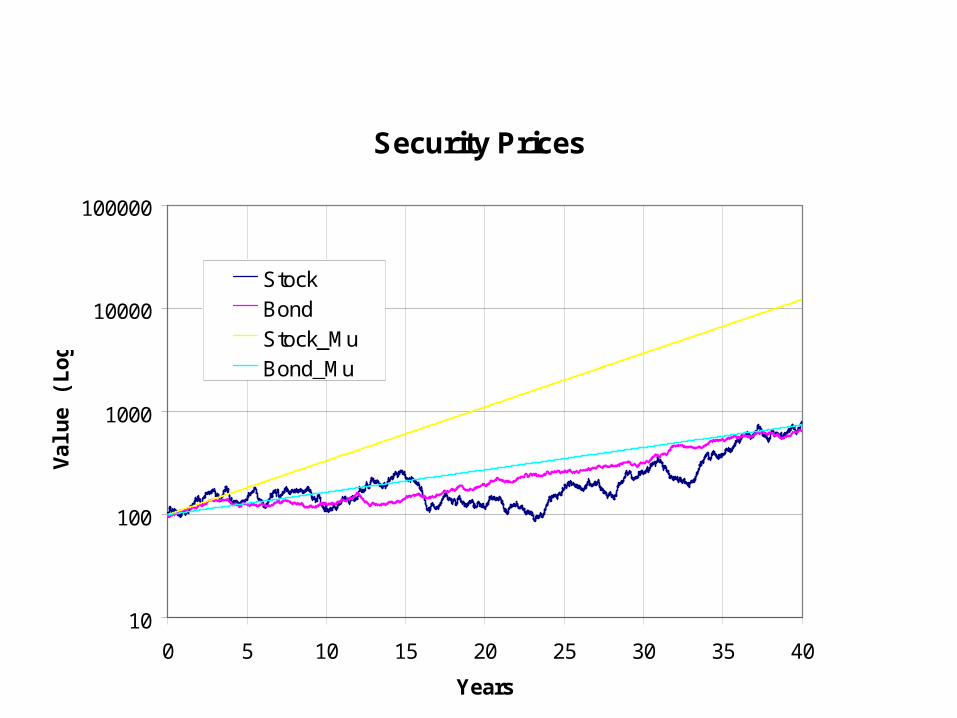
Price Trajectories

• The following graph show the the price of the two securities generated by a bivariate normal distribution for returns– The more risky security may be thought of as a

share of common stock or a stock mutual fund– The less risky security may be thought of as a

bond or a bond mutual fund

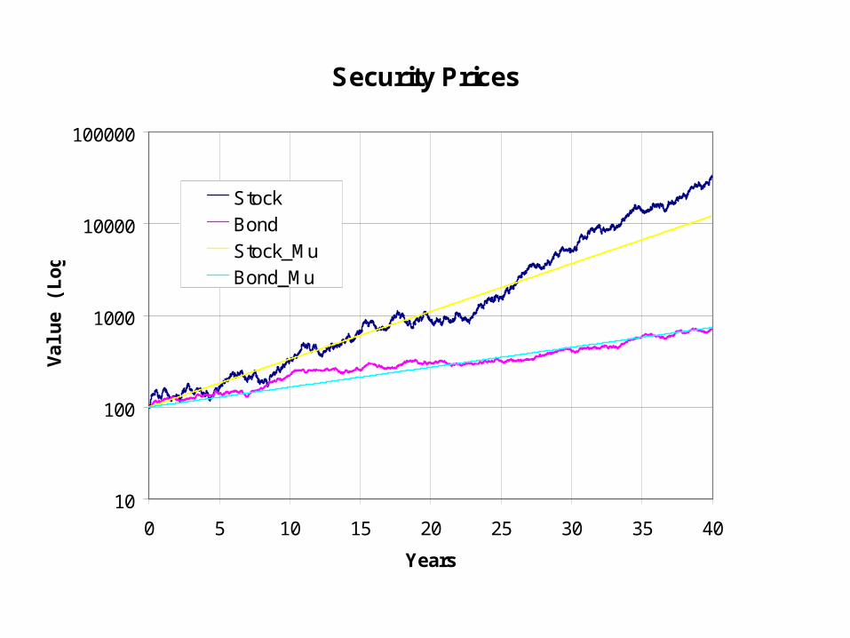
Security Prices

10

100

1000

10000

100000

0 5 10 15 20 25 30 35 40

Years

Val

ue

(Lo

g)

StockBond

Stock_MuBond_Mu

Interpretation of the Graph

• The graph is plotted on a log scale in so that you can see the important features

• The magenta bond trajectory is clearly less risky than the navy-blue stock trajectory

• The expected prices of the bond and the stock are straight lines on a log scale

Interpretation of the Graph

• Recall the log scale: the volatility increases with the length of the investment

• You begin to form the conjecture that the chances of the stock price being less than the price bond is higher in earlier years

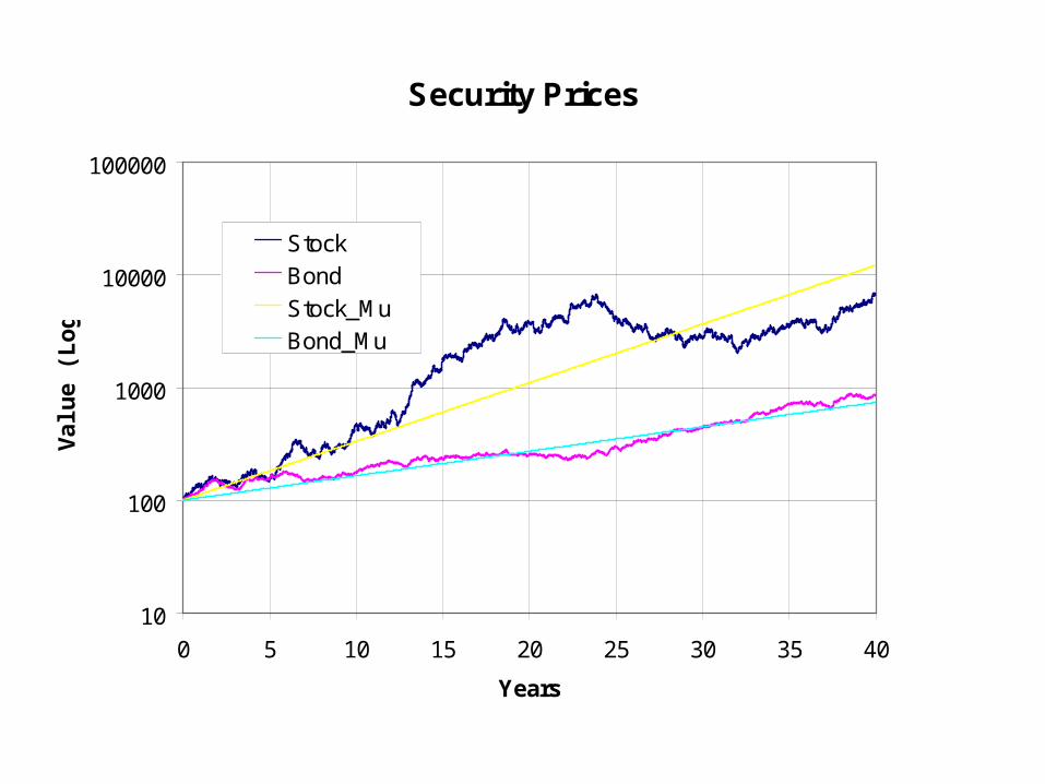
Generating More Trajectories

• This was just one of an infinite number of trajectories generated by the same 2 means, 2 volatilities, and the correlation– I have not cheated you, this was indeed the first

trajectory generated by the statistics– the following trajectories are not reordered nor

edited• Instructor: On slower computers there may be a delay

Security Prices

10

100

1000

10000

100000

0 5 10 15 20 25 30 35 40

Years

Val

ue

(Lo

g)

StockBond

Stock_MuBond_Mu

Security Prices

10

100

1000

10000

100000

0 5 10 15 20 25 30 35 40

Years

Val

ue

(Lo

g)

StockBond

Stock_MuBond_Mu

…and Lots More!Security Prices

10

100

1000

10000

100000

0 5 10 15 20 25 30 35 40

Years

Val

ue

(Lo

g)

StockBondStock_MuBond_Mu

Security Prices

10

100

1000

10000

100000

0 5 10 15 20 25 30 35 40

Years

Val

ue

(Lo

g)

StockBond

Stock_MuBond_Mu

Security Prices

10

100

1000

10000

100000

0 5 10 15 20 25 30 35 40

Years

Val

ue

(Lo

g)

StockBond

Stock_MuBond_Mu

Security Prices

10

100

1000

10000

100000

0 5 10 15 20 25 30 35 40

Years

Val

ue

(Lo

g)

StockBond

Stock_MuBond_Mu

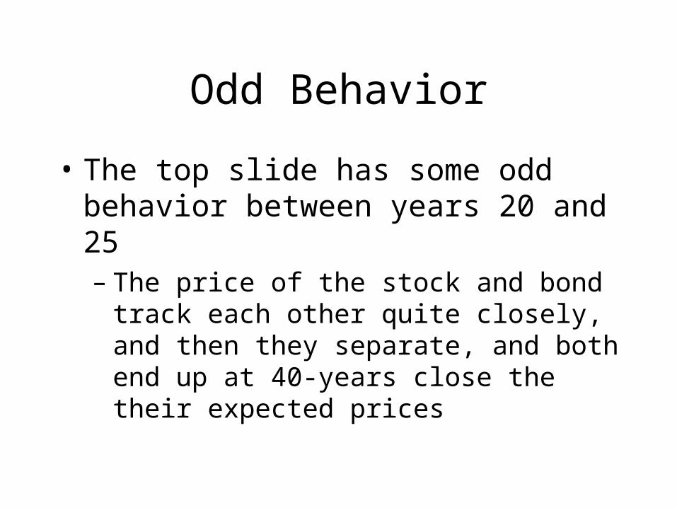
Odd Behavior

• The top slide has some odd behavior between years 20 and 25– The price of the stock and bond track each

other quite closely, and then they separate, and both end up at 40-years close the their expected prices

From Conjecture to Hypothesis

• You are probably ready to make the hypothesis that– the probability of the high-risk, high-return

security will out-perform the low-risk, low-return increases with time

But:

• I promised to be perfectly frank and honest (pfah) with you about the ordering of the simulated trajectories

• The next trajectory truly was the next trajectory in the sequence, honest!

Security Prices

10

100

1000

10000

100000

0 5 10 15 20 25 30 35 40

Years

Val

ue

(Lo

g)

StockBond

Stock_MuBond_Mu

Explanation

• The bond and the stock end up at about the same price, when the expected prices are more than a magnitude apart

• There is either a very good explanation for this, or there is a very high probability that I have been much less than perfectly frank and honest with you

Another View of the Model

• A little mathematics, and we are able to generate the following price distributions for the stock and the bond for 2, 5, 10, and 40 years into the future

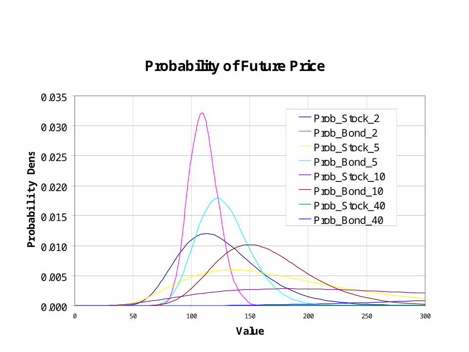
Probability of Future Price

0.000

0.005

0.010

0.015

0.020

0.025

0.030

0.035

0 50 100 150 200 250 300

Value

Pro

bab

ilit

y D

ensi

ty

Prob_Stock_2Prob_Bond_2Prob_Stock_5Prob_Bond_5Prob_Stock_10Prob_Bond_10Prob_Stock_40Prob_Bond_40

• There is a lot going on here, so we will further constrain our view

• First look at stock prices over a period of 10 years

• The prices are distributed according to the lognormal distribution

Probabilistic Stock Price Changes Over Time

0.000

0.002

0.004

0.006

0.008

0.010

0.012

0.014

0.016

0.018

0.020

0 200 400 600 800

Price

Pro

bab

ilit

y D

ensi

ty

Stock_Year_1Stock_Year_2Stock_Year_3Stock_Year_4Stock_Year_5Stock_Year_6Stock_Year_7Stock_Year_8Stock_Year_9Stock_Year_10

Note

– the scale is $0 to $800– the distribution diffuses and drifts towards

higher prices with time– the diffusion is more pronounced in the earlier

years than in the later years– you may see that the mode, median, and mean

appear to drift apart with time

Bond in Time

• You will recall that if you invest in a 5-year default-free pure discount bond for 5 years, the return is known with certainty

• To avoid this effect, assume we invest in short term bonds, and roll them over as they mature

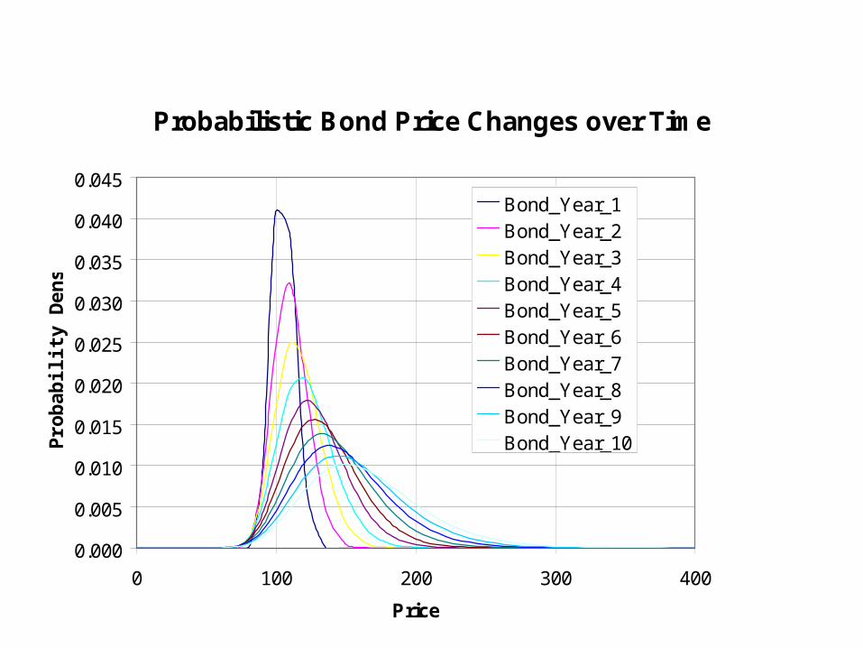
Probabilistic Bond Price Changes over Time

0.000

0.005

0.010

0.015

0.020

0.025

0.030

0.035

0.040

0.045

0 100 200 300 400

Price

Pro

bab

ilit

y D

ensi

ty

Bond_Year_1Bond_Year_2Bond_Year_3Bond_Year_4Bond_Year_5Bond_Year_6Bond_Year_7Bond_Year_8Bond_Year_9Bond_Year_10

Note

– the scale is now $0 to $400 (not $0 to $800 as in the case of the stock)

– we observe the same kind of diffusion and drift behavior, and there is less of each

• (remember to adjust for the scale)

Contrast of Trajectories and Distributions

• The price distributions and the trajectories were generated from the same distribution. But

• They do not seem to agree– The distributions appear to produce much lower

averages (expected returns) than the trajectories

Meaty Tails

• The resolution is that the distributions have much meatier tails than your intuition allows, pushing the median and mean further and further from the mode with time

• The region where the left tail appears to have drifted into insignificance has a profound affect on the mean

Stock and Bonds Distributions Compared at the Same Times

• The next sequence of slides contrasts the distribution of stock and bond prices at 1, 2, 5, 10, and 40 into the future

• Some of the slides have different measures of central tendency indicated

• Note the behavior of these statistics as time increases

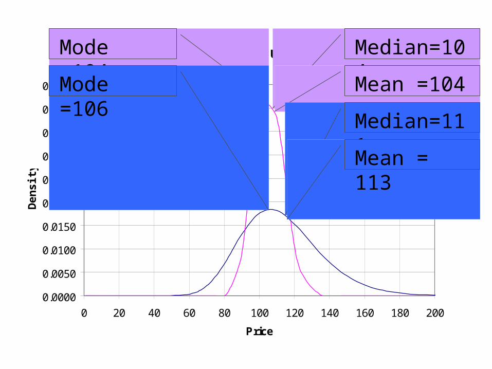
1-Year Out

0.0000

0.0050

0.0100

0.0150

0.0200

0.0250

0.0300

0.0350

0.0400

0.0450

0 20 40 60 80 100 120 140 160 180 200

Price

Den

sity

Stock_1_YearBond_1_Year

Mode =104Mode =106

Median=104Mean =104Median=111Mean = 113

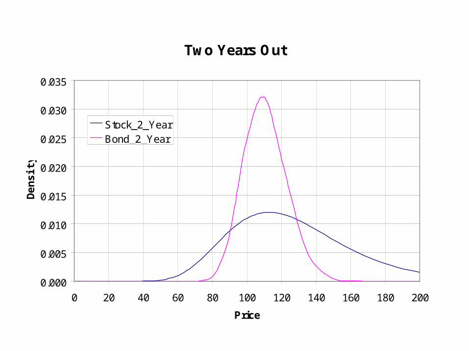
Two Years Out

0.000

0.005

0.010

0.015

0.020

0.025

0.030

0.035

0 20 40 60 80 100 120 140 160 180 200

Price

Den

sity

Stock_2_YearBond_2_Year

5-Years Out

0.000

0.002

0.004

0.006

0.008

0.010

0.012

0.014

0.016

0.018

0.020

0 100 200 300 400 500

Price

Den

sity

Stock_5_YearBond_5_Year

Mode = 122

Mode = 135

Median= 126Mean = 128

Median= 165Mean = 182

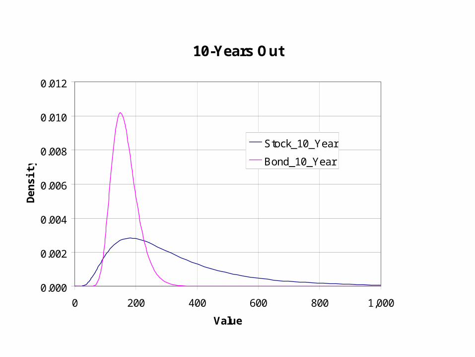
10-Years Out

0.000

0.002

0.004

0.006

0.008

0.010

0.012

0 200 400 600 800 1,000

Value

Den

sity

Stock_10_Year

Bond_10_Year

40 Years Out

0.000

0.000

0.000

0.001

0.001

0.001

0.001

0.001

0.002

0 5,000 10,000 15,000 20,000 25,000 30,000

Value

Den

sity

Stock_40_YearBond_40_Year

Mode =503

Mode =1,102

Median=650

Mean =739

Median=5,460Mean =12,151