chapter 11 nonlinear regression models - nyu

Chapter 11

Nonlinear Regression Models

Exercises 1. We cannot simply take logs of both sides of the equation as the disturbance is additive rather than multiplicative. So, we must treat the model as a nonlinear regression. The linearized equation is y ≈ α α α α ββ β β0 0 00 0 0

x x x x+ − + −( ) (log ) ( β0 )where α0 and β0 are the expansion point. For given values of α0 and β0, the estimating equation would be

( ) ( )y x + ε* x x x x x x− + + = +α α α α β αβ β β β β0 0 0 00 0 0 0 0(log ) (log )

or ( ) ( )y x x x x x+ = +α α β αβ β0 00 0(log ) (log ) β0

+ ε*.

Estimates of α and β are obtained by applying ordinary least squares to this equation. The process is repeated with the new estimates in the role of α0 and β0. The iteration could be continued until convergence. Starting values are always a problem. If one has no particular values in mind, one candidate would be α0 = y and β0 =

0 or β0 = 1 and α0 either x′y/x′x or y / x . Alternatively, one could search directly for the α and β to minimize the sum of squares, S(α,β) = Σi (yi - αxβ)2 = Σi εi

2. The first order conditions for minimization are ∂S(α,β)/∂α = -2Σi (yi - αxβ)xβ = 0 and ∂S(α,β)/∂β = -2Σi (yi - αxβ)α(lnx)xβ = 0. Methods for solving nonlinear equations such as these are discussed in Appendix E.. 2. The proof can be done by mathematical induction. For convenience, denote the ith derivative by fi. The first derivative appears in Equation (10-34). Just by plugging in i=1, it is clear that f1 satisfies the relationship. Now, use the chain rule to differentiate f1, f2 = (-1/λ2)[xλ(lnx) - x(λ)] + (1/λ)[(lnx)xλ(lnx) - f1] Collect terms to yield f2 = (-1/λ)f1 + (1/λ)[xλ(lnx)2 - f1] = (1/λ)[xλ(lnx)2 - 2f1]. So, the relationship holds for i = 0, 1, and 2. We now assume that it holds for i = K-1, and show that if so, it also holds for i = K. This will complete the proof. Thus, assume fK-1 = (1/λ)[xλ(lnx)K-1 - (K-1)fK-2] Differentiate this to give fK = (-1/λ)fK-1 + (1/λ)[(lnx)xλ(lnx)K-1 - (K-1)fK-1]. Collect terms to give fK = (1/λ)[xλ(lnx)K - KfK-1], which completes the proof for the general case. Now, we take the limiting value limλ→0 fi = limλ→0 [xλ(lnx)i - ifi-1]/λ. Use L'Hospital's rule once again. limλ→0 fi = limλ→0 d{[xλ(lnx)i - ifi-1]/dλ}/limλ→0 dλ/dλ. Then, limλ→0 fi = limλ→0 {[xλ(lnx)i+1 - ifi]} Just collect terms, (i+1)limλ→0 fi = limλ→0 [xλ(lnx)i+1] or limλ→0 fi = limλ→0 [xλ(lnx)i+1]/(i+1) = (lnx)i+1/(i+1).

80

Applications 1. First, the two simple regressions produce Linear Log-linear Constant 114.338 1.17064 (173.4) (.3268) Labor 2.33814 .602999 (1.039) (.1260) Capital .471043 .37571 (.1124) (.08535) R2 .9598 .9435 Standard Error 469.86 .1884 In the regression of Y on 1, K, L, and the predicted values from the loglinear equation minus the predictions from the linear equation, the coefficient on α is -587.349 with an estimated standard error of 3135. Since this is not significantly different from zero, this evidence favors the linear model. In the regression of lnY on 1, lnK, lnL and the predictions from the linear model minus the exponent of the predictions from the loglinear model, the estimate of α is .000355 with a standard error of .000275. Therefore, this contradicts the preceding result and favors the loglinear model. An alternative approach is to fit the Box-Cox model in the fashion of Exercise 4. The maximum likelihood estimate of λ is about -.12, which is much closer to the log-linear model than the lonear one. The log-likelihoods are -192.5107 at the MLE, -192.6266 at λ=0 and -202.837 at λ = 1. Thus, the hypothesis that λ = 0 (the log-linear model) would not be rejected but the hypothesis that λ = 1 (the linear model) would be rejected using the Box-Cox model as a framework. 2. The search for the minimum sum of squares produced the following results:

λ e′e -.500 .78477 -.400 .67033 -.300 .60587 -.250 .59479 -.245 .59451 -.244 .59447 -.243 .59444 -.242 .59441 -.241 .59439 -.240 .59438 -.239 .59437 -.238 .59436 -.237 .59437 -.235 .59440 -.225 .59492 -.200 .59897 -.100 .65598 0.000 .78143 .100 .97742

.200 1.24354

81

The sum of squared residuals is minimized at λ = -.238. At this value, the regression results are as follows: Parameter Estimate OLS Std.Error Correct Std.Error α 2.06092 .07718 .09723 βk .178232 .04638 .04378 βl .737988 .06996 .12560 λ -.238 ---- .07710 Estimated Asymptotic Covariance Matrix α βk βl λ α .00945 βk .00262 .00192 βl .00511 -.00199 .01578 λ .00500 .00037 .00825 .00594 The output elasticities for this function evaluated at the sample means are ∂lnY/∂lnK = βkKλ = (.178232).175905-.238 = .2695 ∂lnY/∂lnL = βlLλ = (.443954).737988-.238 = .7740. The estimates found for Zellner and Revankar's model were .254 and .882, respectively, so these are quite similar. For the simple log-linear model, the corresponding values are .2790 and .927. 3. The Wald test is based on the unrestricted model. The statistic is the square of the usual t-ratio, W = (-.232 / .0771)2 = 9.0546. The critical value from the chi-squared distribution is 3.84, so the hypothesis that λ = 0 can be rejected. The likelihood ratio statistic is based on both models. The sum of squared residuals for both unrestricted and restricted models is given above. The log-likelihood is lnL = -(n/2)[1 + ln(2π) + ln(e′e/n)], so the likelihood ratio statistic is LR = n[ln(e′e/n)|λ=0 - ln(e′e/n)| λ=-.238] = nln[(e′e|λ=0) / (e′e|λ=-.238) = 25ln(.78143/.54369) = 6.8406. Finally, to compute the Lagrange Multiplier statistic, we regress the residuals from the log-linear regression on a constant, lnK, lnL, and (1/2)(bkln2K + blln2L) where the coefficients are those from the log-linear model (.27898 and .92731). The R2 in this regression is .23001, so the Lagrange multiplier statistic is LM = nR2 = 25(.23001) = 5.7503. All three statistics suggest the same conclusion, the hypothesis should be rejected. 4. Instead of minimizing the sum of squared deviations, we now maximize the concentrated log-likelihood function, lnL = -(n/2)ln(1+ln(2π)) + (λ - 1)Σi lnYi - (n/2)ln(ε′ε/n). The search for the maximum of lnL produced the results on the next page The log-likelihood is maximized at λ = .124. At this value, the regression results are as follows: Parameter Estimate OLS Std.Error Correct Std.Error α 2.59465 .1283 .7151 βk .378094 .1070 .3228 βl 1.13653 .1117 .4121 λ .124 ---- .2482 σ2 .036922 ---- .0179 Estimated Asymptotic Covariance Matrix α βk βl λ σ2 α .5114 βk .2203 .1042 βl .2612 .0951 .1698 λ .1747 .0730 .0953 .0617 σ2 .0104 .0044 .0059 .0038 .00032

82

λ lnL -.200 -13.6284 -.150 -12.8568 -.100 -12.2423 -.050 -11.7764 0.000 -11.4476 .050 -11.2427 .100 -11.1480 .110 -11.1410 .120 -11.1378 .121 -11.1377 .122 -11.1376 .123 -11.1376 .124 -11.1375 .125 -11.1376 .130 -11.1383 .140 -11.1423 .200 -11.2344 .300 -11.6064 .400 -12.8371

The output elasticities for this function evaluated at the sample means, K = .175905, L = .737988, Y = 2.870777, are ∂lnY/∂lnK = bk(K/Y)λ = .2674 ∂lnY/∂lnL = bl(L/Y)λ = .9017. These are quite similar to the estimates given above. The sum of the two output elasticities for the states given in the example in the text are given below for the model estimated with and without transforming the dependent variable. Note that the first of these makes the model look much more similar to the Cobb Douglas model for which this sum is constant. State Full Box-Cox Model lnQ on left hand side Florida 1.2840 1.6598 Louisiana 1.2019 1.4239 California 1.1574 1.1176 Maryland 1.1657 1.0261 Ohio 1.1899 .9080 Michigan 1.1604 .8506 Once again, we are interested in testing the hypothesis that λ = 0. The Wald test statistic is W = (.123 / .2482)2 = .2455. We would now not reject the hypothesis that λ = 0. This is a surprising outcome. The likelihood ratio statistic is based on both models. The sum of squared residuals for the restricted model is given above. The sum of the logs of the outputs is 19.29336, so the restricted log-likelihood is lnL0 = (0-1)(19.29336) - (25/2)[1 + ln(2π) + ln(.781403/25)] = -11.44757. The likelihood ratio statistic is -2[ -11.13758 - (-11.44757)] = .61998. Once again, the statistic is small. Finally, to compute the Lagrange multiplier statistic, we now use the method described in Example 11.8. The result is LM = 1.5621. All of these suggest that the log-linear model is not a significant restriction on the Box-Cox model. This rather peculiar outcome would appear to arise because of the rather substantial reduction in the log-likelihood function which occurs when the dependent variable is transformed along with the right hand side. This is not a contradiction because the model with only the right hand side transformed is not a parametric restriction on the model with both sides transformed. Some further evidence is given in the next exercise.

83

5. --> nlsq ; lhs = y ; labels = b1,b2 ; fcn=b1*(1 - 1/sqr(1+2*b2*x)) ; start = 500,.0001 ;output=2$ Begin NLSQ iterations. Linearized regression. Iteration= 1; Sum of squares= 11603.0164 ; Gradient= 11602.9326 Iteration= 2; Sum of squares= 19821.5463 ; Gradient= 19821.4534 Iteration= 3; Sum of squares= 331169.005 ; Gradient= 331144.576 Iteration= 4; Sum of squares= 356630.271 ; Gradient= 356504.582 Iteration= 5; Sum of squares= 14997.8506 ; Gradient= 14938.8590 Iteration= 6; Sum of squares= 449.855530 ; Gradient= 442.701921 Iteration= 7; Sum of squares= 102026.884 ; Gradient= 102026.775 Iteration= 8; Sum of squares= 12887.7536 ; Gradient= 12886.6539 Iteration= 9; Sum of squares= 14263101.5 ; Gradient= 14263101.0 Iteration= 10; Sum of squares= 10203.1920 ; Gradient= 10202.6789 Iteration= 11; Sum of squares= 144.393444 ; Gradient= 144.338425 Iteration= 12; Sum of squares= 258.186688 ; Gradient= 258.145522 Iteration= 13; Sum of squares= .154284512 ; Gradient= .113316151 Iteration= 14; Sum of squares= .409681292E-01; Gradient= .129216769E-05 Iteration= 15; Sum of squares= .409668370E-01; Gradient= .439070450E-13 Iteration= 16; Sum of squares= .409668370E-01; Gradient= .211594637E-18 Iteration= 17; Sum of squares= .409668370E-01; Gradient= .107898463E-24 Convergence achieved +----------------------------------------------------+ | Nonlinear least squares regression | | LHS=Y Mean = 43.34071 | | Standard deviation = 22.80652 | | WTS=none Number of observs. = 14 | | Model size Parameters = 2 | | Degrees of freedom = 12 | | Residuals Sum of squares = .4096684E-01 | | Standard error of e = .5409439E-01 | | Fit R-squared = .9999939 | | Not using OLS or no constant. Rsqd & F may be < 0. | +----------------------------------------------------+ +--------+--------------+----------------+--------+--------+ |Variable| Coefficient | Standard Error |b/St.Er.|P[|Z|>z]| +--------+--------------+----------------+--------+--------+ B1 | 636.427250 4.31789336 147.393 .0000 B2 | .00020814 .164134D-05 126.809 .0000 --> nlsq ; lhs = y ; labels = b1,b2 ; fcn=b1*(1 - 1/sqr(1+2*b2*x)) ; start = 600,.0002 ;output=2$ Begin NLSQ iterations. Linearized regression. Iteration= 1; Sum of squares= 262.456583 ; Gradient= 262.415454 Iteration= 2; Sum of squares= .155984704 ; Gradient= .115016579 Iteration= 3; Sum of squares= .409675977E-01; Gradient= .760690867E-06 Iteration= 4; Sum of squares= .409668370E-01; Gradient= .379981726E-13 Iteration= 5; Sum of squares= .409668370E-01; Gradient= .186919870E-18 Iteration= 6; Sum of squares= .409668370E-01; Gradient= .150578559E-23 Convergence achieved +----------------------------------------------------+ | Nonlinear least squares regression | | LHS=Y Mean = 43.34071 | | Standard deviation = 22.80652 | | Residuals Sum of squares = .4096684E-01 | | Standard error of e = .5409439E-01 | | Fit R-squared = .9999939 | | Adjusted R-squared = .9999944 | +----------------------------------------------------+ +--------+--------------+----------------+--------+--------+ |Variable| Coefficient | Standard Error |b/St.Er.|P[|Z|>z]| +--------+--------------+----------------+--------+--------+ B1 | 636.427250 4.31789336 147.393 .0000 B2 | .00020814 .164134D-05 126.809 .0000

84

Chapter 12

Instrumental Variables Estimation

Exercises 1. There is no need for a separate proof different from the usual for OLS. Formally, however, it follows from the results at (12-4) that

b = 1

n n

−′ ′⎛ ⎞ ⎛+ ⎜ ⎟ ⎜⎝ ⎠ ⎝

X X X ⎞⎟⎠

εβ

Then,

1

1plim n n

−−′ ′⎛ ⎞ ⎛ ⎞− = −⎜ ⎟ ⎜ ⎟

⎝ ⎠ ⎝ ⎠XX

X X Xb b Qε γ

and

( )1

1plim n nn n

−−

⎡ ⎤′ ′⎛ ⎞ ⎛ ⎞− = −⎢ ⎥⎜ ⎟ ⎜ ⎟⎝ ⎠ ⎝ ⎠⎢ ⎥⎣ ⎦

XXX X Xb b Qε γ

The large sample distribution of this statistic will be the same as the large sample of the statistic with X′X/n replaced with its probablity limit, which is QXX. Thus,

( ) 1plim n nn

− ′⎡ ⎤⎛ ⎞− → −⎜ ⎟⎢ ⎥⎝ ⎠⎣ ⎦XX

Xb b Q ε γ

To deduce the large sample behavior of this statistic, we can invoke the results from chapter 4. The only change here is the nonzero mean (probability limit) of the vector in brackets. [See (12-3).] Thus, the same proof applies. The consistency, asymptotic normality and asymptotic covariance matrix equal to Asy.Var[b] = σε

2 (X′X)-1 2. A logical solution to this one is simple. For y and x*, Cov2(y,x*)/[Var(y)Var(x*)] = β2(σ*

2)2/[(β2σ*2+σε

2)(σ*2)]

Cov2(y,x) /[Var(y)Var(x)] = Cov[βx*+ε,x*+u] / [Var(y)Var(x)] = {Cov[y,x*] +Cov[y,u]}2 / [Var(y)Var(x)] . The second term is zero, since y=βx*+ε which is uncorrelated with u. Thus, Cov2(y,x) /[Var(y)Var(x)] = Cov[y,x*] / [Var(y)Var(x)]. The numerator is the same. The denominator is larger, since [Var(y)Var(x)] = Var[y](Var[x*] + Var[u]), so the squared correlation must be smaller. If both variables are measured with errors, then we are comparing Cov2(y*,x*)/{Var[y*]Var[x*]} to Cov2(y,x)/{Var[y]Var[x]}. The numerator is the covariance of (βx* + ε + v) with (x* + u), so the numerator of the fraction is still β2(σ*

2)2. The denominator is still obviously larger, so the same result holds when both variables are measured with error. 3. We work off (12-16), using repeatedly the result Σuu = (σuj)(σuj)′ where j has a 1 in the first position and 0 in the remaining K-1. From (12-16), plim b = β - [Q* + Σuu]-1Σuuβ. The vector is Σuuβ equals [σu

2β1,0,...,0]′. The inverse matrix is

[Q* + Σuu]-1 = ( )( )

( ) ( )1 11

1* * ( )( ) *1 ( ) * ( )

u uu u

− −

−

⎡ ⎤′− σ⎢ ⎥

′+ σ σ⎢ ⎥⎣ ⎦Q Q j

j Q j1−σ j Q

85

This can be simplified since the quadratic form in the denominator just picks off the 1,1 diagonal element. Thus,

[Q* + Σuu]-1 = ( ) ( ) ( )1 12 *11

1* * ( )( ) *1 u u

uq− −⎡ ⎤

′− σ σ⎢ ⎥+ σ⎣ ⎦Q Q j j 1−Q

Then

[Q* + Σuu]-1Σuuβ= ( ) ( ) ( )1 1 1−Q ( )( )u u2 *11

1* * ( )( ) *1 u u

uq− −⎡ ⎤

′− σ σ⎢ ⎥+ σ⎣ ⎦Q Q j j ′σ σj j β

= ( ) 1* −Q ( )( )u u ′σ σj j β - ( ) ( )1 12 *11

1 * ( )( ) *1 u u

uq− −′σ σ

+ σQ j j Q ( )( )u u ′σ σj j β

= ( j σu2β1 - ) 1* −Q ( )

2 *111 2

12 *11 * 1

uu

u

qq

−σσ β

+σQ j

= ( j ) 1* −Q2 *11

2 *1111

u

u

qq

⎡ ⎤σ−⎢ ⎥+σ⎣ ⎦

σu2β1

= ( j ) 1* −Q 2 *11

11 uq⎡ ⎤⎢ ⎥+ σ⎣ ⎦

σu2β1

= ( j ) 1* −Q2

12 *111

u

uq⎡ ⎤σ β⎢ ⎥+ σ⎣ ⎦

Finally, j equals the first column of (( ) 1* −Q ) 1* −Q = [q*11, q*21,...,q*k1]. Therefore, the first element, given by (12-17a) is

plim b1 = β1 - 2

12 *111

u

uq⎡ ⎤σ β⎢ + σ⎣ ⎦

⎥ q*11 = β1

2 *11

2 *1111

u

u

qq

⎡ ⎤σ−⎢ ⎥+σ⎣ ⎦

For (12-17b),

plim b2 = β2 - 2

12 *111

u

uq⎡ ⎤σ β⎢ ⎥+ σ⎣ ⎦

q*k1

4. To obtain the result, note first: plim b = β + QXX

-1γ Asy.Var[b] = (σ2/n)QXX

-1 Asy.Var[b2sls] = (σ2/n)QZX

-1QZZQXZ-1.

86

The mean squared error of the OLS estimator is the variance plus the squared bias, M(b|β) = (σ2/n)QXX

-1 + QXX-1γγ′QXX

-1 the mean squared error of the 2SLS estimator equals its variance. For OLS to be more precise then 2SLS, we would have to have (σ2/n)QXX

-1 + QXX-1γγ′QXX

-1 << (σ2/n)QZX-1QZZQXZ

-1. For convenience, let δ = QXX

-1γ so M(b|β) = (σ2/n)QXX-1 + δδ′. If the mean squared error matrix of the

OLS estimator is smaller than that of the 2SLS estimator, then its inverse is larger. Use (A-66) to do the inversion. The result would be [(σ2/n)QXX

-1 + δδ′]-1 >> [(σ2/n)QZX-1QZZQXZ

-1]-1 Now, use A-66

[(σ2/n)QXX-1 + δδ′]-1 = (n/σ2) QXX - 2

11 ( / )n′+ σ XXQδ δ

(n/σ2) QXXδδ′(n/σ2) QXX

Reinsert δ = QXX-1γ and the right hand side above reduces to

(n/σ2) QXX - 2

11 ( / )n ′+ σ -1

XXQγ γ(n/σ2)2 γγ′

Therefore, if the mean squared error matrix of OLS is smaller, then

(n/σ2) QXX - 2

11 ( / )n ′+ σ -1

XXQγ γ(n/σ2)2 γγ′ >> (n/σ2)QXZQZZ

-1QZX

Collect the terms, and this implies

(n/σ2)[ QXX - QXZQZZ-1QZX] >> 2

11 ( / )n ′+ σ -1

XXQγ γ(n/σ2)2 γγ′

divide both sides by (n/σ2),

QXX - QXZQZZ-1QZX >>

2

2

( / )1 ( / )

nn

σ′+ σ -1

XXQγ γγγ′

and divide numerator and denominator of the fraction by n/σ2

QXX - QXZQZZ-1QZX >> 2

1( / )n ′σ + -1

XXQγ γγγ′

which is the desired result. Is it possible? It is possible, since QXX - QXZQZZ

-1QZX = plim (1/n)[X′X - X′Z(Z′Z)-1Z′X] = plim (1/n) X′MZX which is a positive definite matrix. SInce γ varies independently of Z and X, certainly there is some configuration of the data and parameters for which this is the case. The result is that it is, indeed, possible for OLS to be more precise, in the mean squared error sense, than 2SLS. 5. The matrices are X = [i,x] and Z = [i,z]. For the OLS estimators, we know from chapter 2 that a = y bx− and b = Cov[x,y]/var[x]. For the IV estimator, (Z′X)-1Z′y, we obtain the result in detail. Given the forms,

1 11

1 1 1 1 1 1 1 11

1( ) , ( ) , ( )

i

z i

n x n nx n x nx nyn x n n x n n n ynn x x

−

=

Σ −⎡ ⎤ ⎡ ⎤ ⎡ ⎤ ⎡′ ′= = = =⎢ ⎥ ⎢ ⎥ ⎢ ⎥ ⎢Σ −−⎣ ⎦ ⎣ ⎦ ⎣⎣ ⎦Z X Z X Z y

⎤′ ⎥⎦

where subscript 1 indicates the mean of the observations for which z equals 1, and n1 is the number of observations. Multiplying the matrix times the vector and cancelling terms produces the solutions

aIV = 1 1 1

1 1

and IV IVx y x y y y

a bx x x− −

= =− − x

87

Application a. The statement of the problem is actually a bit optimistic. GIven the way it is stated, it would imply that the exogenous variables in the “demand” equation would be, in principle, (Ed, Union, Fem) which are also in the supply equation, plus the remainder, (Exp, Exp2, Occ, Ind, South, SMSA, Blk). The problem is that the model as stated would not be identified – the supply equation would, but the demand equation would not be. The way out would be to assume that at least one of (Ed, Union, Fem) does not appear in the demand equation. Since surely education would, that leaves one or both of Union and Fem. We will assume both of them are omitted. So, our equation is lnWageit = α1 + α2Edit + α3Expit + α4Expit

2 + α5Occit + α6Indit + α7Southit + α8SMSAit + α9Blkit + γ Wksit + uit. NAMELIST ; X = one,Ed,Exp,Expsq,Occ,Ind,South,SMSA,Blk,Wks $ NAMELIST ; Z = one,Ed,Exp,expsq,Occ,Ind,south,SMSA,Blk,Union,Fem $ Regress ; Lhs = lwage ; Rhs = X $ 2SLS ; Lhs = lwage ; Rhs = X ; Inst = Z $ REGRESS ; Lhs = Wks ; Rhs = Z ; cls:b(10)=0,b(11)=0$ +----------------------------------------------------+ | Ordinary least squares regression | | LHS=LWAGE Mean = 6.676346 | | Standard deviation = .4615122 | | WTS=none Number of observs. = 4165 | | Model size Parameters = 10 | | Degrees of freedom = 4155 | | Residuals Sum of squares = 581.2717 | | Standard error of e = .3740280 | | Fit R-squared = .3446066 | | Adjusted R-squared = .3431870 | | Model test F[ 9, 4155] (prob) = 242.74 (.0000) | +----------------------------------------------------+ +--------+--------------+----------------+--------+--------+----------+ |Variable| Coefficient | Standard Error |b/St.Er.|P[|Z|>z]| Mean of X| +--------+--------------+----------------+--------+--------+----------+ Constant| 5.13171052 .07238152 70.898 .0000 ED | .06112766 .00277226 22.050 .0000 12.8453782 EXP | .04291665 .00229783 18.677 .0000 19.8537815 EXPSQ | -.00070803 .506204D-04 -13.987 .0000 514.405042 OCC | -.07814434 .01502100 -5.202 .0000 .51116447 IND | .09066812 .01247863 7.266 .0000 .39543818 SOUTH | -.07629062 .01318346 -5.787 .0000 .29027611 SMSA | .13789225 .01278553 10.785 .0000 .65378151 BLK | -.26269494 .02304380 -11.400 .0000 .07226891 WKS | .00484184 .00113470 4.267 .0000 46.8115246 +----------------------------------------------------+ | Two stage least squares regression | | LHS=LWAGE Mean = 6.676346 | | Standard deviation = .4615122 | | WTS=none Number of observs. = 4165 | | Model size Parameters = 10 | | Degrees of freedom = 4155 | | Residuals Sum of squares = 602.3138 | | Standard error of e = .3807377 | | Fit R-squared = .3192467 | | Adjusted R-squared = .3177722 | | Model test F[ 9, 4155] (prob) = 216.50 (.0000) | +----------------------------------------------------+ | Instrumental Variables: |ONE ED EXP EXPSQ OCC IND SOUTH SMSA |BLK UNION FEM +--------+--------------+----------------+--------+--------+----------+ |Variable| Coefficient | Standard Error |b/St.Er.|P[|Z|>z]| Mean of X| +--------+--------------+----------------+--------+--------+----------+ Constant| 4.46105888 .27680953 16.116 .0000 ED | .06167266 .00283031 21.790 .0000 12.8453782

88

EXP | .04207640 .00236282 17.808 .0000 19.8537815 EXPSQ | -.00068241 .525268D-04 -12.992 .0000 514.405042 OCC | -.07605669 .01531301 -4.967 .0000 .51116447 IND | .08348143 .01302032 6.412 .0000 .39543818 SOUTH | -.08242895 .01364036 -6.043 .0000 .29027611 SMSA | .13244624 .01319402 10.038 .0000 .65378151 BLK | -.25212290 .02383132 -10.579 .0000 .07226891 WKS | .01922950 .00583960 3.293 .0010 46.8115246 This is the test of relevance of the instrumental variables. In the regression of WKS on the full set of exogenous variables, we test the hypothesis that the coefficients on the instruments, UNION and FEM are jointly zero. The results show that the hypothesis is rejected. We conclude that the instruments are relevant. +----------------------------------------------------+ | Linearly restricted regression | | Ordinary least squares regression | | LHS=WKS Mean = 46.81152 | | Standard deviation = 5.129098 | | WTS=none Number of observs. = 4165 | | Model size Parameters = 9 | | Degrees of freedom = 4156 | | Residuals Sum of squares = 108653.5 | | Standard error of e = 5.113097 | | Fit R-squared = .8138966E-02 | | Adjusted R-squared = .6229705E-02 | | Model test F[ 8, 4156] (prob) = 4.26 (.0000) | | Restrictns. F[ 2, 4154] (prob) = 84.57 (.0000) | | Not using OLS or no constant. Rsqd & F may be < 0. | | Note, with restrictions imposed, Rsqd may be < 0. | +----------------------------------------------------+ +--------+--------------+----------------+--------+--------+----------+ |Variable| Coefficient | Standard Error |b/St.Er.|P[|Z|>z]| Mean of X| +--------+--------------+----------------+--------+--------+----------+ Constant| 46.6129896 .67547781 69.007 .0000 ED | -.03787988 .03789322 -1.000 .3175 12.8453782 EXP | .05840099 .03139904 1.860 .0629 19.8537815 EXPSQ | -.00178055 .00069145 -2.575 .0100 514.405042 OCC | -.14509978 .20533021 -.707 .4798 .51116447 IND | .49950389 .17041135 2.931 .0034 .39543818 SOUTH | .42663864 .18010107 2.369 .0178 .29027611 SMSA | .37851979 .17468415 2.167 .0302 .65378151 BLK | -.73479892 .31481083 -2.334 .0196 .07226891 UNION | .444089D-15 .182255D-08 .000 1.0000 .36398559 FEM | .000000 ......(Fixed Parameter).......

89

Chapter 13 ⎯⎯⎯⎯⎯⎯⎯⎯⎯⎯⎯⎯⎯⎯⎯⎯⎯⎯⎯⎯⎯⎯⎯⎯⎯⎯⎯⎯⎯⎯⎯⎯⎯⎯⎯⎯⎯⎯⎯⎯⎯⎯⎯

Simultaneous Equations Models 1. (a) Since nothing is excluded from either equation and there are no other restrictions, neither equation passes the order condition for identification. (1) We use (13-12) and the equations which follow it. For the first equation, [A3′,A5′] = β22, a scalar which has rank M-1 = 1 unless β22 = 0. For the second, [A3′,A5′] = β31. Thus, both equations are identified. (2) This restriction does not restrict the first equation, so it remains unidentified. The second equation is now identified, as [A3′,A5′] = [β11,β21] has rank 1 if either of the two ceofficients are nonzero. (3) If γ1 equals 0, the model becomes partially recursive. The first equation becomes a regression which can be estimated by ordinary least squares. However, the second equation continues to fail the order condition. To see the problem, consider that even with the restriction, any linear combination of the two equations has the same variables as the original second eqation. (4) We know from above that if β32 = 0, the second equation is identifiable. If it is, then γ2 is identified. We may treat it as known. As such, γ1 is known. By regressing y1 - γ1y2 on the xs, we would obtain estimates of the remaining parameters, so these restrictions identify the model. It is instructive to analyze this from the standpoint of false structures as done in the text. A false structure which incorporates

the known restrictions would be × . If the false structure is to obey the restrictions,

then f11 - γ f21 = 1, f22 - γ f12 = 1, f21 - γf11 = f12 - γ f22, β31 f12 = 0. It follows then that f12 = 0 so f11 = 1. Then, f21 - γf 11 = -γ or f21 = (f11 - 1)γ so that f11 - γ2(f11 - 1) = 1. This can only hold for all values of γ if f11 = 1 and, then, f21 = 0. Therefore, F = I which establishes identification.

11

0

11 12

21 22

31

−−⎡

⎣

⎢⎢⎢⎢⎢⎢

⎤

⎦

⎥⎥⎥⎥⎥⎥

γλ

β ββ ββ

f ff f11 12

21 22

⎡

⎣⎢

⎤

⎦⎥

(5) If β31 = 0, the first equation is identified by the usual rank and order conditions. Consider, then, the off-diagonal element of Σ = Γ′ΩΓ. Ω is identified since it is the reduced form covariance matrix. The off-diagonal element is σ12 = ω11 + ω22 - (γ1 + γ2)ω12 = 0. Since γ1 is zero, γ2 = ω12/(ω11 + ω22). With γ2 known, the remaining parameters are estimable by least squares regression of (y2 - γ2y1) on the xs. Therefore, the restrictions identify the model. (6) Since this is only a single restriction, it will not likely identify the entire model. Consider again the false structure. The restrictions implied by the theory are f11 - γ2f21 = 1, f22 - γ1f12 = 1, β21f11 + β22f21 = β21f12 + β22f22. The three restrictions on four unknown elements of F do not serve to pin down any of them. This restriction does not even partially identify the model. (7) The last four restrictions remove x2 and x3 from the model. The remaining model is not identified by the usual rank and order conditions. From part (5), we see that the first restriction implies σ12 = ω11 + ω22 - (γ1 + γ2)ω12 = 0. But, with neither γ1 nor γ2 specified, this does not identify either parameter. (8) The first equation is identified by the conventional rank and order conditions. The second equation fails the order condition. But, the restriction σ12 = 0 provides the necessary additional information needed to identify the model. For simplicity, write the model with the restrictions imposed as y1 = γ1y2 + ε1 and y2 = γ2y1 + βx + ε2. The reduced form is y1 = π1x + v1 and y2 = π2x + v2 where π1 = γ1β/Δ and π2 = β/Δ with Δ = (1 - γ1γ2), and v1 = (ε1 + γ1ε2)/Δ and v2 = (ε2 + γ2ε1)/Δ. The reduced form variances and covariances are ω11 = (γ1

2σ22 + σ11)/Δ2, ω22 = (γ22σ11 + σ22)/Δ2, ω12 = (γ1σ22 + γ2σ11)/Δ2.

All reduced form parameters are estimable directly by using least squares, so the reduced form is identified in all cases. Now, γ1 = π1/π2. σ11 is the residual variance in the euqation (y1 - γ1y2) = ε1, so σ11 must be estimable (identified) if γ1 is. Now, with a bit of manipulation, we find that γ1ω12 - ω11 = -σ11/Δ. Therefore, with σ11 and

90

γ1 "known" (identified), the only remaining unknown is γ2, which is therefore identified. With γ1 and γ2 in hand, β may be deduced from π2. With γ2 and β in hand, σ22 is the residual variance in the equation (y2 - βx - γ2y1) = ε2, which is directly estimable, therefore, identified. 2. Following the method in Example 13.6, for identification of the investment equation, we require that the

matrix have rank 5. Columns (1), (4), (6), (7), and (8) each

have one element in a different row, so they are linearly independent. Therefore, the matrix has rank five. For

the third equation, the required matrix is . Columns

(4), (6), (7), (9), and (10) are linearly independent.

( ) ( ) ( ) ( ) ( ) ( ) ( ) ( ) ( )1 2 3 4 5 6 7 8 91 0 0 0 0 0 0

0 1 0 0 0 00 0 1 0 0 1 0 0 00 1 1 0 0 0 1 0 00 0 0 1 0 0 0 0 0

3 3

1

−−

−− −

⎡

⎣

⎢⎢⎢⎢⎢⎢⎢⎢

⎤

⎦

⎥⎥⎥⎥⎥⎥⎥⎥

α αγ γ 3 2γ

3β

12

41 42

21

52

γγ γβ

β

⎡

⎣

⎢⎢⎢⎢

⎤

⎦

⎥⎥⎥⎥

1 0

0 0

12

31 32 33

52

γβ β β

β

⎡

⎣

⎢⎢⎢

⎤

⎦

⎥⎥⎥

( ) ( ) ( ) ( ) ( ) ( ) ( ) ( ) ( ) ( )1 2 3 4 5 6 7 8 9 101 0 0 0 0 0 0

0 1 0 0 0 0 01 1 0 0 0 01 0 0 0 00 0 1 0 0 0 1 0 0 00 1 0 1 0 0 0 0 0 1

1 3 2

1 2

−−

− −−

⎡

⎣

⎢⎢⎢⎢⎢⎢⎢⎢

⎤

⎦

⎥⎥⎥⎥⎥⎥⎥⎥

α α αβ β

3. We find [A3′,A5′]′ for each equation. (1) (2) (3) (4) γ γβ β β

β ββ

32 34

12 13 14

43 4

32

1

00 0

⎡

⎣

⎢⎢⎢⎢

⎤

⎦

⎥⎥⎥⎥

, [ ] , , 0 43 44β β

1 01

1 00 00

Identification requires that the rank of each matrix be M-1 = 3. The second is obviously not identified. In (1), none of the three columns can be written as a linear combination of the other two, so it has rank 3. (Although the second and last columns have nonzero elements in the same positions, for the matrix to have short rank, we would require that the third column be a multiple of the second, since the first cannot appear in the linear combination which is to replicate the second column.) By the same logic, (3) and (4) are identified. 4. Obtain the reduced form for the model in Exercise 1 under each of the assumptions made in parts (a) and (b1), (b6), and (b9). (1). The model is y1 = γ1y2 + β11x1 + β21x2 + β31x3 + ε1 y2 = γ2y1 + β12x1 + β22x2 + β32x3 + ε2.

Therefore, Γ = and B = and Σ is unrestricted. The reduced form is 1

12

1

−−⎡

⎣⎢

⎤

⎦⎥

γγ

− −−

−

⎡

⎣

⎢⎢⎢

⎤

⎦

⎥⎥⎥

β ββ

β

11 12

22

31

00

Π= 11 1 2

11 1 21 2 11 12

1 22 22

31 2 31−

+ +⎡

⎣

⎢⎢⎢

⎤

⎦

⎥⎥⎥

γ γ

β γ β γ β βγ β ββ γ β

and

91

Ω = (Γ-1)′Σ(Γ-1) = 11

2

2

1 22

11 12

22

1 12

2 11 1 22

1 2 12

2 11 1 22

1 2 12

22

11 22

1 12

( )

( )

( )

−

++

++ +

++ +

++

⎡

⎣

⎢⎢⎢⎢⎢⎢

⎤

⎦

⎥⎥⎥⎥⎥⎥

γ γ

σ γ σγ σ

γ σ γ σγ γ σ

γ σ γ σγ γ σ

γ σ σγ σ

(6) The model is y1 = β11x1 + β21x2 + β31x3 + ε1 y2 = γ2y1 + β12x1 + β22x2 + β32x3 + ε2 The first equation is already a reduced form. Substituting it into the second provides the second reduced form.

The coefficient matrix is P= , Γ-1 = so Ω = (Γ-1)′Σ(Γ-1) = β β γ ββ β γ ββ β γ β

11 12 2 11

21 22 2 21

31 32 2 31

+++

⎡

⎣

⎢⎢⎢

⎤

⎦

⎥⎥⎥

10 1

2γ⎡

⎣⎢

⎤

⎦⎥

σ γ σγ σ γ σ σ

11 2 11

2 11 22

11 22+⎡

⎣⎢

⎤

⎦⎥

(9) The model is y1 = γ1y2 + ε1 y2 = γ2y1 + β12x1 + ε2

Then, Π = -BΓ-1 = [β12γ1/(1-γ1γ2) β12/(1-γ1γ2)] and Ω = . σ γ σ γ σ γ σγ σ γ σ γ σ σ

11 12

22 2 11 1 22

2 11 1 22 22

11 22

+ ++ +

⎡

⎣⎢⎢

⎤

⎦⎥⎥

5. The relevant submatrices are X′X = , X′y1 = , X′y2 = , y1′y1 = 20, y2′y2 = 10,

y1′y2 = 6, X′Z1 = , X′Z2 = Z1′Z1 = , Z2′Z2 = ,

5 2 32 10 83 8 15

⎡

⎣

⎢⎢⎢

⎤

⎦

⎥⎥⎥

435

⎡

⎣

⎢⎢⎢

⎤

⎦

⎥⎥⎥

367

⎡

⎣

⎢⎢⎢

⎤

⎦

⎥⎥⎥

3 56 27 3

⎡

⎣

⎢⎢⎢

⎤

⎦

⎥⎥⎥

4 2 33 10 85 8 15

⎡

⎣

⎢⎢⎢

⎤

⎦

⎥⎥⎥

10 33 5

⎡

⎣⎢

⎤

⎦⎥

10 3 53 10 85 8 15

⎡

⎣

⎢⎢⎢

⎤

⎦

⎥⎥⎥

Z1′Z2 = , Z1′y1 = , Z1′y2 = , Z2′y1 = , Z2′y2 = . 6 6 74 2 3⎡

⎣⎢

⎤

⎦⎥

64⎡

⎣⎢⎤

⎦⎥

103

⎡

⎣⎢

⎤

⎦⎥

2035

⎡

⎣

⎢⎢⎢

⎤

⎦

⎥⎥⎥

667

⎡

⎣

⎢⎢⎢

⎤

⎦

⎥⎥⎥

The two OLS coefficient vectors are d1 = (X′X)-1X′y1 = [.439024,.536585] ′ d2 = (X′X)-1X′y2 = [.193016,.384127,.19746] ′. The two stage least squares estimators are

= [Z1′X(X′X)-1X′Z1]-1[Z1′X(X′X)-1X′y1] = [.368816,.578711] ′. δ∧

1

= [Z2′X(X′X)-1X′Z2]-1[Z2′X(X′X)-1X′y2] = [.484375,.367188,.109375] ′. δ∧

2

= (y1′y1 - 2y1′Z + δ ′Z1′Z1 ) / 25 = .610397, = .268384. σ∧

11 δ∧

1∧

1 δ∧

1 σ∧

22

The estimated asymptotic covariance matrices are

Est.Var[ ] = [Z1′X(X′X)-1X′Z1]-1 = δ∧

1 σ∧

11. .. .215858 129035129036 1995⎡

⎣⎢

⎤

⎦⎥

Est.Var[Est.Var[ ]] = . δ∧

2

. . .. . .. . .

132423 007699 040035007688 047259 022538040035 022638 043311

− −− −− −

⎡

⎣

⎢⎢⎢

⎤

⎦

⎥⎥⎥

The three stage least squares estimate is

92

σ σ

σ σ

σ

σ

σ

111

11

121

12

122

11

222

12

1

111

11

121

12

122

11

∧−

∧−

∧−

∧−

−

∧−

∧−

∧−

⎡

⎣

⎢⎢⎢

⎤

⎦

⎥⎥⎥

+

[ ' ( ' ) ' ] [ ' ( ' ) ' ]

[ ' ( ' ) ' ] [ ' ( ' ) ' ]

[ ' ( ' ) ' ]

[ ' ( ' ) ' ]

[ ' ( ' ) ' ]

Z X X X X Z Z X X X X Z

Z X X X X Z Z X X X X Z

Z X X X X y

Z X X X X y

Z X X X X y +

⎡

⎣

⎢⎢⎢⎢⎢⎢⎢⎢⎢⎢

⎤

⎦

⎥⎥⎥⎥⎥⎥⎥⎥⎥⎥

∧−σ22

21

2[ ' ( ' ) ' ]Z X X X X Z

= [.368817,.578708,.4706,.306363,.168294]′ . The estimated standard errors are the square roots of the diagonal elements of the inverse matrix, [.4637,.4466,.3626,.1716,.1628], compared to the 2SLS values, [.4637,.4466,.3639,.2174,.2081]. To compute the limited information maximum likelihood estimator, we require the matrix of sums of squares and cross products of residuals of the regressions of y1 and y2 on x1 and on x1, x2, and x3. These are

W0 = Y′Y - Y′x1(x1′x1)-1x1′Y = , W1 = Y′Y - Y′X(X′X)-1X′Y = 165 360360 8 20

. .. .

⎡

⎣⎢

⎤

⎦⎥

16 2872 255312255312 53617

. .. .

.⎡

⎣⎢

⎤

⎦⎥

The two characteristic roots of (W1)-1W0 are 1.53157 and 1.00837. We carry the smaller one into the k-class computation [see, for example, Theil (1971) or Judge, et al (1985)];

δ∧

1k = 10 100837 53617 3

3 56 100837 255312

436711657973

1−⎡

⎣⎢

⎤

⎦⎥

−⎡

⎣⎢

⎤

⎦⎥ =

⎡

⎣⎢

⎤

⎦⎥

−. ( . ) . ( . ) ..

Finally, the two estimates of the reduced form are

(OLS) P = . .. .. .

680851 329787010638 37243191489 202128

⎡

⎣

⎢⎢⎢

⎤

⎦

⎥⎥⎥

and (2SLS) . Π∧ −

=−

−−

⎡

⎣

⎢⎢⎢

⎤

⎦

⎥⎥⎥

−⎡

⎣⎢

⎤

⎦⎥ =

⎡

⎣

⎢⎢⎢

⎤

⎦

⎥⎥⎥

...

.. .. .. .

578711 00 3671880 109375

1 484375704581 341281104880 447051049113 133164

1

-.368816 1

6. For the model y1 = γ1y2 + β11x1 + β21x2 + ε1 y2 = γ2y1 + β32x3 + β42x4 + ε2 show that there are two restrictions on the reduced form coefficients. Describe a procedure for estimating the model while incorporating the restrictions.

The structure is [y1 y2] 1

1 00

2

11 2 3 4 1 1

−−⎡

⎣⎢

⎤

⎦⎥ +

⎡

⎣

⎢⎢⎢⎢

⎤

⎦

⎥⎥⎥⎥

=γ

γ

ββ

ββ

ε ε[ [x x x x ]

00

11

21

32

42

].

or y′ Γ + x′B = ε′. The reduced form coefficient matrix is

Π = -BΓ-1 = 11 1 2

11 2 11

21 2 21

1 32 32

1 42 42

−

⎡

⎣

⎢⎢⎢⎢

⎤

⎦

⎥⎥⎥⎥

γ γ

β γ ββ γ βγ β βγ β β

= The two restrictions are π12/π11 = π22/π21 and

π31/π32 = π41/π42. If we write the reduced form as

π ππ ππ ππ π

11 21

21 22

31 32

41 42

⎡

⎣

⎢⎢⎢⎢

⎤

⎦

⎥⎥⎥⎥

y1 = π11x1 + π21x2 + π31x3 + π41x4 + v1 y2 = π12x1 + π22x2 + π32x3 + π42x4 + v2. We could treat the system as a nonlinear seemingly unrelated regressions model. One possible way to handle the restrictions is to eliminate two parameters directly by making the substitutions π12 = π11π22/π21 and π31 = π32π41/π42.

93

The pair of equations would be y1 = π11x1 + π21x2 + (π32π41/π42)x3 + π41x4 + v1 y2 = (π11π22/π21)x1 + π22x2 + π32x3 + π42x4 + v2. This nonlinear system could now be estimated by nonlinear GLS. The function to be minimized would be Σ i vi1

2σ11 + vi2n=1

2

−

σ22 + 2vi1vi2σ12 = ntr(Σ-1W). Needless to say, this would be quite involved. 7. We would require that all three characteristic roots have modulus less than one. An intuitive guess that the diagonal element greater than one would preclude this would be correct. The roots are the solutions to

det− − − −

−− −

⎡

⎣

⎢⎢⎢

⎤

⎦

⎥⎥⎥

. . ..

. . .

1899 9471 89910 10287 0

0656 0791 0952

λλ

λ= 0. Expanding this produces -(.1899 + λ)(1.0287 - λ)(.0952 - λ)

- .0565(1.0287 - λ).8991 = 0. There is no need to go any further. It is obvious that λ = 1.0287 is a solution, so there is at least one characteristic root larger than 1. The system is unstable. 8. Prove plim Yj′ε/T = ωj - Ωjjγj. Consistent with the partitioning y′ = [yj Yj′ Yi

*′], partition Ω into ωjj ωj′ ω*

j′ Ω = ωj Ωjj Ωj′ ω*

j Ω*j Ωj

*

and, as in the equation preceding (13-8), partition the jth column of Γ as Γj = . Since the full set of

reduced form disturbances is V = EΓ-1, it follows that E = VΓ. In particular, the jth column of E is εj = VΓj. In the reduced form, now referring to (15-8), Yj = XΠj + Vj, where Πj is the Mj columns of Π corresponding to the included endogenous variables and Vj is the T×Mj matrix of their reduced form disturbances. Since X is uncorrelated with all columns of E, we have

1−⎡

⎣

⎢⎢⎢

⎤

⎦

⎥⎥⎥

γ0

plim Yj′εj/T = plim Vj′ Γj /T = [ωj Ωjj Ωj* ] = ωj - Ωjjγj as required. 1−⎡

⎣

⎢⎢⎢

⎤

⎦

⎥⎥⎥

γ0

9. Prove that an underidentified equation cannot be estimated by two stage least squares. If the equation fails the order condition, then the number of excluded exogenous variables is less than the number of included endogenous. The matrix of instrumental variables to be used for two stage least

squares is of the form Z = [XA,Xj], where XA is Mj linear combination of all K columns in X and Xj is Kj

columns of X. In total, K = Kj* + Kj. If the equation fails the order condition, then Kj

* < Mj, so Z is Mj + Kj

columns which are linear combinations of K = Kj* + Kj < Mj + Kj. Therefore, cannot have full column

rank. In order to compute the two stage least squares estimator, we require ( ′ )-1, which cannot be computed.

∧

∧

Z∧

Z∧

Z∧

94

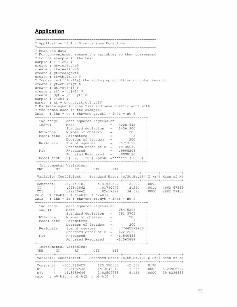
Application ?========================================================= ? Application 13.1 - Simultaneous Equations ?========================================================= ? Read the data ? For convenience, rename the variables so they correspond ? to the example in the text. sample ; 1 - 204 $ create ; ct=realcons$ create ; it=realinvs$ create ; gt=realgovt$ create ; rt=tbilrate $ ? Impose (artifically) the adding up condition on total demand. create ; yt=ct+it+gt $ create ; ct1=ct[-1] $ create ; yt1 = yt[-1] $ create ; dyt = yt - yt1 $ sample ; 2-204 $ names ; xt = one,gt,rt,ct1,yt1$ ? Estimate equations by 2sls and save coefficients with ? the names used in the example. 2sls ; lhs = ct ; rhs=one,yt,ct1 ; inst = xt $ +----------------------------------------------------+ | Two stage least squares regression | | LHS=CT Mean = 3008.995 | | Standard deviation = 1456.900 | | WTS=none Number of observs. = 203 | | Model size Parameters = 3 | | Degrees of freedom = 200 | | Residuals Sum of squares = 75713.32 | | Standard error of e = 19.45679 | | Fit R-squared = .9998208 | | Adjusted R-squared = .9998190 | | Model test F[ 2, 200] (prob) =******* (.0000) | +----------------------------------------------------+ | Instrumental Variables: |ONE GT RT CT1 YT1 +--------+--------------+----------------+--------+--------+----------+ |Variable| Coefficient | Standard Error |b/St.Er.|P[|Z|>z]| Mean of X| +--------+--------------+----------------+--------+--------+----------+ Constant| -13.8657181 5.31536302 -2.609 .0091 YT | .05843862 .01790473 3.264 .0011 4663.67389 CT1 | .92200662 .02657199 34.698 .0000 2982.97438 calc ; a0=b(1) ; a1=b(2) ; a2=b(3) $ 2sls ; lhs = it ; rhs=one,rt,dyt ; inst = xt $ +----------------------------------------------------+ | Two stage least squares regression | | LHS=IT Mean = 654.5296 | | Standard deviation = 391.3705 | | WTS=none Number of observs. = 203 | | Model size Parameters = 3 | | Degrees of freedom = 200 | | Residuals Sum of squares = .7744227E+08 | | Standard error of e = 622.2631 | | Fit R-squared = -1.540485 | | Adjusted R-squared = -1.565889 | +----------------------------------------------------+ | Instrumental Variables: |ONE GT RT CT1 YT1 +--------+--------------+----------------+--------+--------+----------+ |Variable| Coefficient | Standard Error |b/St.Er.|P[|Z|>z]| Mean of X| +--------+--------------+----------------+--------+--------+----------+ Constant| -300.699429 125.980850 -2.387 .0170 RT | 56.5192542 15.4643912 3.655 .0003 5.24965517 DYT | 16.5359646 2.02509785 8.166 .0000 39.8236453 calc ; b0=b(1) ; b1=b(2) ; b2=b(3) $

95

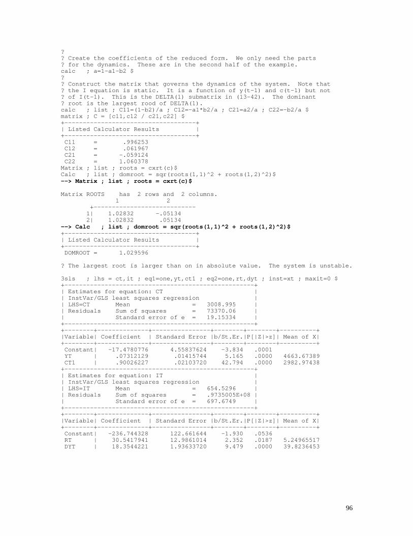
? ? Create the coefficients of the reduced form. We only need the parts ? for the dynamics. These are in the second half of the example. calc ; a=1-a1-b2 $ ? ? Construct the matrix that governs the dynamics of the system. Note that ? the I equation is static. It is a function of y(t-1) and c(t-1) but not ? of I(t-1). This is the DELTA(1) submatrix in (13-42). The dominant ? root is the largest rood of DELTA(1). calc ; list ; C11=(1-b2)/a ; C12=-a1*b2/a ; C21=a2/a ; C22=-b2/a $ matrix ; C = [c11,c12 / c21,c22] $ +------------------------------------+ | Listed Calculator Results | +------------------------------------+ C11 = .996253 C12 = .061967 C21 = -.059124 C22 = 1.060378 Matrix ; list ; roots = cxrt(c)$ Calc ; list ; domroot = sqr(roots(1,1)^2 + roots(1,2)^2)$ --> Matrix ; list ; roots = cxrt(c)$ Matrix ROOTS has 2 rows and 2 columns. 1 2 +---------------------------- 1| 1.02832 -.05134 2| 1.02832 .05134 --> Calc ; list ; domroot = sqr(roots(1,1)^2 + roots(1,2)^2)$ +------------------------------------+ | Listed Calculator Results | +------------------------------------+ DOMROOT = 1.029596 ? The largest root is larger than on in absolute value. The system is unstable. 3sls ; lhs = ct,it ; eq1=one,yt,ct1 ; eq2=one,rt,dyt ; inst=xt ; maxit=0 $ +----------------------------------------------------+ | Estimates for equation: CT | | InstVar/GLS least squares regression | | LHS=CT Mean = 3008.995 | | Residuals Sum of squares = 73370.06 | | Standard error of e = 19.15334 | +----------------------------------------------------+ +--------+--------------+----------------+--------+--------+----------+ |Variable| Coefficient | Standard Error |b/St.Er.|P[|Z|>z]| Mean of X| +--------+--------------+----------------+--------+--------+----------+ Constant| -17.4780776 4.55837624 -3.834 .0001 YT | .07312129 .01415744 5.165 .0000 4663.67389 CT1 | .90026227 .02103720 42.794 .0000 2982.97438 +----------------------------------------------------+ | Estimates for equation: IT | | InstVar/GLS least squares regression | | LHS=IT Mean = 654.5296 | | Residuals Sum of squares = .9735005E+08 | | Standard error of e = 697.6749 | +----------------------------------------------------+ +--------+--------------+----------------+--------+--------+----------+ |Variable| Coefficient | Standard Error |b/St.Er.|P[|Z|>z]| Mean of X| +--------+--------------+----------------+--------+--------+----------+ Constant| -236.744328 122.661644 -1.930 .0536 RT | 30.5417941 12.9861014 2.352 .0187 5.24965517 DYT | 18.3544221 1.93633720 9.479 .0000 39.8236453

96

Chapter 14 ⎯⎯⎯⎯⎯⎯⎯⎯⎯⎯⎯⎯⎯⎯⎯⎯⎯⎯⎯⎯⎯⎯⎯⎯⎯⎯⎯⎯⎯⎯⎯⎯⎯⎯⎯⎯⎯⎯⎯⎯⎯⎯⎯

Estimation Frameworks in Econometrics

Exercise 1. A fully parametric model/estimator provides consistent, efficient, and comparatively precise results. The semiparametric model/estimator, by comparison, is relatively less precise in general terms. But, the payoff to this imprecision is that the semiparametric formulation is more likely to be robust to failures of the assumptions of the parametric model. Consider, for example, the binary probit model of Chapter 21, which makes a strong assumption of normality and homoscedasticity. If the assumptions are correct, the probit estimator is the most efficient use of the data. However, if the normality assumption or the homoscedasticity assumption are incorrect, then the probit estimator becomes inconsistent in an unknown fashion. Lewbel’s semiparametric estimator for the binary choice model, in contrast, is not very precise in comparison to the probit model. But, it will remain consistent if the normality assumption is violated, and it is even robust to certain kinds of heteroscedasticity.

Applications 1. Using the gasoline market data in Appendix Table F2.2, use the partially linear regression method in Section 16.3.3 to fit an equation of the form ln(G/Pop) = β1ln(Income) + β2lnPnew cars + β3lnPused cars + g(lnPgasoline) + ε crea;gp=lg;ip=ly;ncp=lpnc;upp=lpuc;pgp=lpg$ sort;lhs=pgp;rhs=gp,ip,ncp,upp$ crea;dgp=.809*gp - .5*gp[-1] - .309*gp[-2]$ crea;dip=.809*ip - .5*ip[-1] - .309*ip[-2]$ crea;dnc=.809*ncp -.5*ncp[-1]-.309*ncp[-2]$ crea;duc=.809*upp -.5*upp[-1]-.309*upp[-2]$ samp;3-36$ regr;lhs=dgp;rhs=dip,dnc,duc;res=e$ +-----------------------------------------------------------------------+ | Ordinary least squares regression Weighting variable = none | | Dep. var. = DGP Mean= .9708646870E-02, S.D.= .4738748109E-01 | | Model size: Observations = 34, Parameters = 3, Deg.Fr.= 31 | | Residuals: Sum of squares= .1485994289E-01, Std.Dev.= .02189 | | Fit: R-squared= .799472, Adjusted R-squared = .78653 | | Model test: F[ 2, 31] = 61.80, Prob value = .00000 | | Diagnostic: Log-L = 83.2587, Restricted(b=0) Log-L = 55.9431 | | LogAmemiyaPrCrt.= -7.559, Akaike Info. Crt.= -4.721 | | Model does not contain ONE. R-squared and F can be negative! | | Autocorrel: Durbin-Watson Statistic = 1.34659, Rho = .32671 | +-----------------------------------------------------------------------+ +---------+--------------+----------------+--------+---------+----------+ |Variable | Coefficient | Standard Error |t-ratio |P[|T|>t] | Mean of X| +---------+--------------+----------------+--------+---------+----------+ DIP .9629902959 .11631885 8.279 .0000 .14504254E-01 DNC -.1010972781 .87755182E-01 -1.152 .2581 .20153536E-01 DUC -.3197058148E-01 .51875022E-01 -.616 .5422 .35656776E-01 --> matr;varpl={1+1/(2*2)}*varb$ --> matr;stat(b,varpl)$ +---------------------------------------------------+

97

|Number of observations in current sample = 34 | |Number of parameters computed here = 3 | |Number of degrees of freedom = 31 | +---------------------------------------------------+ +---------+--------------+----------------+--------+---------+ |Variable | Coefficient | Standard Error |b/St.Er.|P[|Z|>z] | +---------+--------------+----------------+--------+---------+ B_1 .9629902959 .13004843 7.405 .0000 B_2 -.1010972781 .98113277E-01 -1.030 .3028 B_3 -.3197058148E-01 .57998037E-01 -.551 .5815 2. +---------------------------------------+ | Nonparametric Regression for G | | Observations = 36 | | Points plotted = 36 | | Bandwidth = .468092 | | Statistics for abscissa values---- | | Mean = 2.316611 | | Standard Deviation = 1.251735 | | Minimum = .914000 | | Maximum = 4.109000 | | ---------------------------------- | | Kernel Function = Logistic | | Cross val. M.S.E. = 121.084982 | | Results matrix = KERNEL | +---------------------------------------+

Nonparametric Regression for G

PG

80

90

100

110

120

701.00 1.50 2.00 2.50 3.00 3.50 4.00 4.50.50

E[y|xi]G

E[y|

xi]

3. A. Using the probit model and the Klein and Spady semiparametric models, the two sets of coefficient estimates are somewhat similar. +---------------------------------------------+ | Binomial Probit Model | | Maximum Likelihood Estimates | | Model estimated: Jul 31, 2002 at 05:16:40PM.| | Dependent variable P | | Weighting variable None | | Number of observations 601 | | Iterations completed 5 |

98

| Log likelihood function -307.2955 | | Restricted log likelihood -337.6885 | | Chi squared 60.78608 | | Degrees of freedom 5 | | Prob[ChiSqd > value] = .0000000 | | Hosmer-Lemeshow chi-squared = 5.74742 | | P-value= .67550 with deg.fr. = 8 | +---------------------------------------------+ +---------+--------------+----------------+--------+---------+----------+ |Variable | Coefficient | Standard Error |b/St.Er.|P[|Z|>z] | Mean of X| +---------+--------------+----------------+--------+---------+----------+ Index function for probability Z2 -.2202376072E-01 .10177371E-01 -2.164 .0305 32.487521 Z3 .5990084920E-01 .17086004E-01 3.506 .0005 8.1776955 Z5 -.1836462412 .51493239E-01 -3.566 .0004 3.1164725 Z7 .3751312008E-01 .32844576E-01 1.142 .2534 4.1946755 Z8 -.2729824396 .52473295E-01 -5.202 .0000 3.9317804 Constant .9766647244 .36104809 2.705 .0068 +---------------------------------------------+ | Seimparametric Binary Choice Model | | Maximum Likelihood Estimates | | Model estimated: Jul 31, 2002 at 11:01:24PM.| | Dependent variable P | | Weighting variable None | | Number of observations 601 | | Iterations completed 13 | | Log likelihood function -334.7367 | | Restricted log likelihood -337.6885 | | Chi squared 5.903551 | | Degrees of freedom 4 | | Prob[ChiSqd > value] = .2064679 | | Hosmer-Lemeshow chi-squared = 118.69649 | | P-value= .00000 with deg.fr. = 8 | | Logistic kernel fn. Bandwidth = .34423 | +---------------------------------------------+ +---------+--------------+----------------+--------+---------+----------+ |Variable | Coefficient | Standard Error |b/St.Er.|P[|Z|>z] | Mean of X| +---------+--------------+----------------+--------+---------+----------+ Characteristics in numerator of Prob[Y = 1] Z2 -.3284308221E-01 .52254249E-01 -.629 .5297 32.487521 Z3 .1089817386 .86483083E-01 1.260 .2076 8.1776955 Z5 -.2384951835 .23320058 -1.023 .3064 3.1164725 Z7 -.1026067037 .17130225 -.599 .5492 4.1946755 Z8 -.1892263132 .21598982 -.876 .3810 3.9317804 Constant .0000000000 ........(Fixed Parameter)........

99

The first figure below plots the probit probabilities against the Klein and Spady probabilities. The models are obviously similar, though there is substantial difference in the fitted values.

KSPROBS

.10

.20

.30

.40

.50

.60

.70

.80

.00.150 .200 .250 .300 .350 .400 .450.100

PRO

BIT

S

Finally, these two figures plot the predicted probabilities from the two models against the respective index functions, b’x. Note that the two plots are based on different coefficient vectors, so it is not possible to merge the two figures.

101

chapter 11 nonlinear regression models - nyu

Documents