chaotic behavior of soil radon gas and...

Acta Geophysica vol. 64, no. 5, Oct. 2016, pp. 1563-1592

DOI: 10.1515/acgeo-2016-0077

________________________________________________ Ownership: Institute of Geophysics, Polish Academy of Sciences; © 2016 Kamışlıoğlu and Külahcı. This is an open access article distributed under the Creative Commons Attribution-NonCommercial-NoDerivs license, http://creativecommons.org/licenses/by-nc-nd/3.0/.

Chaotic Behavior of Soil Radon Gas and Applications

Miraç KAMIŞLIOĞLU and Fatih KÜLAHCI

Nuclear Physics Division, Department of Physics, Faculty of Science, Fırat University, Elazig, Turkey; e-mail: [email protected]

A b s t r a c t

The soil 222Rn concentration non-linear patterns are investigated by the application of various chaos methodologies based on 70 272 meas-urement data from the East Anatolian Fault Zone, which is one of the world’s most active faults. Among these methodologies are Lyapunov exponent, surrogate data, rescaled range (R/S) analysis, Fourier spec-trum, phase space reconstruction, mutual information, false nearest neighbors, and correlation dimension. The results indicate that the non-linear dynamical approach is convenient for characterization and predic-tion of the 222Rn concentration dynamics, which are in turn usually used as an earthquake precursor. Behaviour of 222Rn gas is important in earth-quake prediction researches.

Key words: chaos, radon, earthquake, time-series, nonlinear analysis.

1. INTRODUCTION Chemically, radon is a moving inactive radioactive element; it is formed by decay of 226Ra, which is produced as a result of radioactive decay of 238U (Durrani and Ilić 1997). Radon occurs as a result of natural radioactive decay of uranium in rocks, soils, and water. Measurements of 222Rn gas concentra-tion have displayed rising concentrations on many fracture and fault zones in soil, air and ground water (Friedmann et al. 1988, Bourai et al. 2013, Chaudhuri et al. 2013, Kumar A. et al. 2013, Lane-Smith and Sims 2013). The presence of radon in an area has been shown through measurements that

M. KAMIŞLIOĞLU and F. KÜLAHCI

1564

vary depending on the geological structure with great importance in soil and groundwater media. They also suggest that 222Rn concentration changes de-pending on the earthquake magnitude and the geological structure of the re-gion. High radon concentration is common in soil under deep cracks such as geological faults and active volcanoes. Cothern and Smith (1987) stated that radon concentration level is strongly affected from geological and geophysi-cal conditions. Various studies have shown convenient signals before and af-ter seismic events (Friedmann et al. 1988, Miklavčić et al. 2008, Külahcı et al. 2009, Kumar N. et al. 2013). There have been different studies along ac-tive faults to understand the importance of radon concentration changes in earthquake mechanisms. An earthquake is expected to increase the mobility of radon gas in the soil (Ulomov and Mavashev 1967, Igarashi and Saeki 1995, King 1986). Some studies have shown that a few weeks or months be-fore occurrence, the earthquake might be sensed due to radon concentration exchange in soil gas (King et al. 1993, Külahcı and Şen 2014). Discrete changes in radon concentration levels are visible as earthquake precursors (King 1986, Fleischer 1981, Fleischer and Magro-Campero 1985).

Radon behaviors are significantly affected by physical rather than chem-ical conditions; therefore, the radon gas concentration level varies greatly with atmospheric interactions such as barometric pressure and rainfall (Cothern and Smith 1987). The concentration levels are associated with me-teorological and hydrological changes, in addition to seismic activity (Külahcı and Şen 2014, Martinelli 2015).

Radon has a short half-life (3.82 days); therefore, its emanation is re-stricted within a few meters. Thus, 222Rn could be transported more quickly than by diffusion or ground water motion in fault zones. 222Rn gas is required also as a carrier fluid (in gaseous or in liquid forms). The 222Rn gas transport could have range of geological region including groundwater or gases such as CO2, CH4, and N2. This process is most effective for 222Rn gas transport (Woith 2015, Chyi et al. 2010), although the transport mechanism has not been found yet. Also, soil 222Rn gas is used in earthquake prediction process, as shown in various studies reported in the literature (King et al. 1993, Planinić et al. 2004). The 222Rn emanation is known along with earthquake occurrences in geological literature (Wakita et al. 1991). All these studies indicated that the behavior of soil 222Rn gas is not linear.

The linear analysis methods are insufficient in solving such complex problems, and it is expected that a non-linear dynamic system may give bet-ter results for analyses and interpretations. These systems are grouped under the umbrella of the chaos theory, and they are useful tools to define the em-bedded irregularities. The changes in the radon gas level along the fault lines have non-linear behaviours and they are used for the earthquake prediction studies (Cuculeanu and Lupu 1996, Albarello et al. 2003, Planinić et al.

CHAOTIC BEHAVIOR OF RADON GAS AND APPLICATIONS

1565

2004, Ghosh et al. 2007, Das et al. 2009, Külahcı et al. 2009, Qiang and Gui-Ming 2012).

In this paper, 70 272 soil 222Rn gas measurements are considered and the chaotic methodologies are searched to predict the non-linear behaviours. The application is performed for data from Kozan and Yakapınar regions near the East Anatolian Fault Zone, Turkey. In order to reduce the noise in the data at Yakapınar region leading to a stationary time series, 10th order FIR filter is applied by Kaiser Window (Namvaran and Negarestani 2015). Non-linear time series analyses are used for extraction of important information about the underlying dynamic system behaviours.

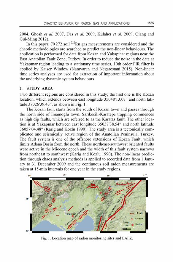
2. STUDY AREA Two different regions are considered in this study; the first one is the Kozan location, which extends between east longitude 35048′13.07′′ and north lati-tude 37026′39.43′′, as shown in Fig. 1.

The Kozan fault starts from the south of Kozan town and passes through the north side of Imamoglu town. Sarıkecili-Karatepe trapping commences as high dip faults, which are referred to as the Karatas fault. The other loca-tion is at Yakapınar between east longitude 35037′38.54′′ and north latitude 36057′04.48′′ (Karig and Kozlu 1990). The study area is a tectonically com-plicated and seismically active region of the Anatolian Peninsula, Turkey. The fault system is one of the offshore extensions of Kozan Fault, which limits Adana Basin from the north. These northeast-southwest oriented faults were active in the Miocene epoch and the width of this fault system narrows from northeast to southwest (Karig and Kozlu 1990). The non-linear predic-tion through chaos analysis methods is applied to recorded data from 1 Janu-ary to 31 December 2009 and the continuous soil radon measurements are taken at 15-min intervals for one year in the study regions.

Fig. 1. Location map of radon monitoring sites and EAFZ.


1566

3. EXPERIMENTAL DATA SET In this study, 222Rn gas is recorded with an alpha detector, Alphameter 611 (Alpha Nuclear Inc. Canada) based on a 400 mm2 silicon junction diode, immersed in a sensing volume open to the geo-gas. In the meantime, it has sensitivity for 1.5 MeV energy levels of continuous monitoring. The data gathered by these sensors are per 15-min unification time. After the disinte-gration of 222Rn gas in the earth, alpha particles emerge and they are detected and the record is kept in the memory of the instrument. It has been stated by Tarakcı et al. (2014) that the Alphameter 611 sensor check is very reliable in continuous soil gas environment with involvements of other ready sensors.

4. METHODS As stated in the abstract of this paper, various non-linear time series analysis techniques are used for the assessment and interpretation of available 222Rn gas concentration measurements.

4.1 Non-linear time series analyses The nature of dynamic systems consists of hidden deterministic and stochas-tic processes. These systems provide opportunity to model trajectory of a dot in a pattern coordinate space, which is equivalent to the phase-space. They can be represented by a series of single records; x1(t), x2(t), …xn(t), in the phase-space. Takens (1981) has shown how to calculate the appropriate pa-rameters for attractor dimension. In the study, time series X(ti), (i = 1, 2, 3, …N) with N number of data point is presented by Xi as an m-dimensional phase-space (m = 1, 2, 3, …) with appropriate delay time τ as

[ ]( ), ( ), L, ( ( 1) )i i i iX X t X t X t m .τ τ= + + − (1)

Herein, m indicates the embedding dimension and τ is the appropriately cho-sen time delay (Chouet and Shaw 1991, Smirnov et al. 2005).

4.2 Surrogate data A chaotic system is a non-linear low-dimensional dynamical mechanism and chaos is a necessary condition for the detection of non-linearity. For a simple chaotic system, it is considerably significant to produce a non-random time series; thus, various methods have been developed to determine the data linearity. The most commonly used technique is surrogate data method, which is based on a statistical approach to determine the linearity of time se-ries. Some linear processes are considered as a null hypothesis. A statistical difference is calculated between surrogate data with original data by generat-ing in accordance with the null hypothesis. As a result of statistical compari-


1567

son, if the value is calculated for the original data, and it is significantly dif-ferent from the value calculated from surrogate data, then null hypothesis is rejected and non-linearity is confirmed (Theiler 1991). Conclusions about whether a time series is chaotic through the test of surrogate data is em-ployed to mimic the statistical properties but with the removal of determin-ism (Theiler et al. 1992). The statistic calculation from raw data should be calculated from the surrogate data too. Theiler (1991) has suggested a meth-odology for non-linearity determinism in time series based on surrogate data, and it seeks evidence for non-linearity by rejecting the null hypothesis of a linear stochastic process. It is important that surrogate data preserve the “lin-ear properties” of the test data. In this study, Theiler methodology is used for surrogated data, because the method of surrogate data distinguishes between linearity and non-linearity as well as between chaotic and pure stochastic properties. Linear stochastic signal can mimic a non-linear chaotic process after a static non-linear distortion (Theiler et al. 1992).

4.3 Lyapunov exponents, λ These exponents, λ, ensure qualitative and quantitative characterizations of dynamic system behavior; they are connected to exponential orbits in the phase space (Wolf 1985). This situation is an initial indicator condition, which is sensitive and depends on chaotic systems. Lyapunov exponent is known as a confident sign to separate a chaotic case from a not chaotic sys-tem (Eckmann and Ruelle 1985, Frazier and Kockelman 2004). The sign gives information about the system dynamics. If the maximum Lyapunov exponent value is λmax > 0, then one can say that it indicates chaos of signa-tures that are received from the dynamics system. On the contrary, if λmax ≤ 0, then it is not a deterministic system. Chaotic situation is very sensi-tive and dependent on the initial conditions. The first algorithms for the cal-culation of Lyapunov exponent from a time series have been presented by Wolf (1985) and Sano and Swada (1985). These methods generate attractor in the phase space of time series by using the approach based on the time de-layed coordinates. Wolf (1985) algorithm depends on finding the maximum Lyapunov exponent with Euclid differences. The method developed by Sano and Sawada (1985) is simple and needs fewer parameters. In this method, average exponential expansion is examined with the distance between neighbor curves on the average (Sano and Sawada 1985, Sato et al. 1987). In his algorithm, the given time series is converted to phase space and the first step to define a Lyapunov exponent is a flux range:

( )x p x= (2)


1568

A trajectory x(t) is defined with a drift from the orbit δ(x). Later con-structions of matrix derivatives ij i jL p x= ∂ ∂ , are found, leading to an equa-tion for the evolving nature of the flux, which can be described as:

( )( )x L x t xδ δ= . (3)

For this reason, in the dynamic system all the initial orbits and initial su-persession have maximum Lyapunov exponent that can be described by the following expression (Eckhardt and Yao 1993)

( )1lim log(0)t

x tt x

δλ

δ∞ →∞= . (4)

In order to calculate the maximum exponent values, Wolf’s method ap-plication is used for the long-term variability throughout a basis axis. This algorithm maintains space orientation using a Gram-Schmidt reortho-normalization procedure (Wolf 1985). Later, the algorithm for Lyapunov ex-ponents is developed by Sano and Sawada (1985) and applied for computing the Lyapunov spectrum. This approach starts with Eqs. 2-4. Furthermore, a linear operator, At, is defined as follows:

( ) (0)tx t A xδ δ= . (5)

If one takes into consideration a given the time series measured at sepa-rate time spacing Δt, xj = x(t0 + (j – 1)Δt), then the k-dimensional ellipsoid, as defined above, can be identified by a replacement vector, yi, and a re-placement vector over a time interval, τ = mΔt, given by zi. How to produce these vectors has been completely summarized in Sano and Sawada (1985). In this method, the evolution of the ellipsoid can be displayed as follows:

i ijz A y= . (6)

Herein, the matrix Aj is an approximation to the flux map At, from Eq. 5. The maximum Lyapunov exponent is calculated by applying the least squares method, which reduces the average of the square error standard de-viations between zi and Ajyi with demonstrations of whole constituent of the matrix Aj (Sano and Sawada 1985). The maximum Lyapunov exponent is computed according to the following expression:

1

1limn

ji j in j

A en

λτ→∞

=

= ∑ , (7)

where n indicates the number of data points, and e is a sequence of or-thonormal basis vectors that are renormalized using the Gram-Schmidt pro-


1569

cedure (Sano and Sawada 1985). This algorithm is established based on the method presented by Sano and Sawada (Sato et al. 1987). The slope of the linear part gives the maximum Lyapunov exponent (Sano and Sawada1985).

4.4 Hurst exponents, H Hurst exponent coefficient is for time series classification (short-term de-pendence or long-term persistence) and it is a statistical measurement tech-nique (Şen 1977a, b, c; Harris et al. 1987). This technique determines long-memory and permits the computation of self-similarity. It is known as re-scaled range (or R/S) method, where R indicates the range of data accumula-tion (that is; given by the difference between the maximum and minimum value) and S shows the standard deviation (Hurst 1951). Hurst exponent is usually used to examine the chaotic behavior or self-similarity of the dy-namic system. The Hurst exponent characterizes the roughness and singular (fractal) character of a signal (shape time series). This study uses discrete time series data {xt} with dimension N. The mean, ( )x N , is as follows

1

1( )N

tt

x N xN =

= ∑ . (8)

The standard deviation S(N) is given by

( )1

22

1

1S( ) ( )N

tt

N x x NN =

⎡ ⎤= −⎢ ⎥⎣ ⎦∑ (9)

Range of cumulative departure of the data is computed by

{ } { }( ) max ( , ) min ( , )R N X n N X n N= − . (10)

Hurst determined the dimensionless ratio R(N)/S(N) as a function of N. Its value falls into the range of 0 and 1, inclusive. In case of any time series as a random signal with finite variance, this ratio increases for large N values as (Feller 1951)

( ) ( ) HR N S N N∝ . (11)

The Hurst exponent can be computed as

( ) / ( ) HR N S N kN= , (12)

where k indicates a constant number. The size of H shows whether the time series is random or consecutive steps in time series are not independent. Hurst exponent is connected to fractal dimension. Thus, fractal dimension is represented with D = 2 – H and correlation between two consecutive steps is given as ρ = 22H–1 – 1 (Feller 1951).


1570

The physical meaning of explanation is necessary for the Hurst exponent in case of the dynamic system. According to this algorithm (Eq. 5), if H = 1/2 then it is called as Hurst exponent and the time series has random walk or white noise (not correlation) form. Hurst exponent indicates that the gradient of the plot of (R/S) versus the time lag N on a double-logarithmic plot is equivalent to H. The H exponent assumes value 0 < H < 1, which are called fractional Brownian motion. For 1/2 < H < 1, the results indicate a permanent movement. Values within 0 < H < 0.5 indicate anti-persistent (negative correlation). Values for H > 1/2 show positive correlation. If H < 1/2, the time series demonstrates anti-persistent behavior (negative cor-relation), where the trajectory tendency is back to the point (Alvarez-Ramirez et al. 2008, Kamışlıoğlu et al. 2013).

4.5 Power spectrum Data from the dynamic system may have little noise for the analysis of sys-tem dynamic. Initially a non-linear time series analysis must be performed by power spectrum analysis. Chaotic signals are very difficult to identify from noise for they have a broad spectrum as noise. Therefore, wide power spectrum indicates the presence of chaos. Power spectrum in a dynamic sys-tem consists of decay peaks as amplitude. The most important criteria in a chaotic form have large band structure (Sprott 2003). Theory of the self-organized critically (SOC) supplies a contact between non-linear dynamics, spatial self-similarity and 1/f noise. It is all over the place and behaves as natural processes in various fields (Gutenberg and Richter 1954, Bak et al. 1988, Crisanti et al. 1992). Power-law distribution implies spatial scale in-variance for any exponent (Sprott 2003). Various studies are carried out for spatially expanding the complex dynamic systems. These systems are known internally and they have characteristic influence in the time domain as 1/f noise. Therefore, power spectrums display a linear behavior on a log-log scale (Bak et al. 1988).

The presence of chaotic signals for a time series can be found also with the power spectrum method, which depends on the frequency of dynamic systems through the power spectrum. If the peaks of the spectrum are con-tinuous, then chaos exists. Power spectrum in the form of random fluctua-tions indicates completely random behavior. Power spectrum S(f) is given as follows:

( )( ) 1S f c f α= , (13)

where S(f) indicates the system power spectral density, f is the frequency, α is a positive real number, and finally c is a constant (Sakata et al. 1999). The


1571

exponent α is predicted with linear regression method application by plotting S(f) versus log(f) (Das et al. 2009).

The power spectrum may appear as noisy in a region of attractors be-longing to a single frequency component. The non-chaotic signal may appear in absence in particular structures. When the system has a narrow-band cha-os then spectrum density shows long and wide peaks in the graph. Thus, the phase space has behavior near a periodic structure. If power spectrum has a broadband chaos, then peaks in the graph are long and wide but this peak is vague.

4.6 Mutual Information Function (MIF) This is a measure of dependence between two random series. The time delay in the mutual information function is proposed by Fraser and Swinney (1986). In contrary to the autocorrelation function, the mutual information function takes into consideration also the non-linear correlations. The mutual information, I(τ), is defined as

( ) ( )( )2

( ), ( )( ) ( ), ( ) ( ), ( ) log

( )) ( ( )P x i x i

I x i x i P x i x iP x i P x i

ττ τ τ

τ⎡ ⎤+

= + + ⎢ ⎥+⎢ ⎥⎣ ⎦

∑ (14)

where P(xi) and P(x(i + τ)) are the marginal probabilities, which are esti-mated typically by relative frequencies. On the other hand, P(xi) and P(x(i + τ)) is the joint probability density that can be computed from two se-ries, namely, x(i) and x(i + τ), where i is a counter. The optimal lag time, τ, minimizes Eq. 6 for t = τ, x(i + τ) and adds the maximum knowledge on x(i) (Khatibi et al. 2012).

4.7 False Nearest Neighbors (FNNs) These help to choose the least embedding dimension of one dimensional time series. Points of the attractor trajectories have neighbors in the phase space and their behavior provides valuable information for understanding the evolution of neighborhood’s in order to produce prediction equations (Abar-banel et al. 1993). When suitable embedding dimension is arrived, then FNN percentage drops to zero. The first step is to reconstruct the phase space from a time set. Hence, an iterative computation defines the local neighborhoods (phase space) and then the count of “false nearest neighbors” dots appears to be close to the nearest neighbors. Every point on the attractor is connected to the orbit X(ti), (i = 1, 2, 3, …N) because embedding space is too small. This approach is used to identify the minimum embedding dimension. The basic idea is to locate dots near each other in the embedded field. These methods help to find the embedding dimension that is rather small and points are near


1572

the embedded space. According to distances, if the calculated ratio is greater than the threshold value, false neighbors appear. If the embedding dimen-sion, m, is very big, then one loses statistics and knowledge (Kennel et al. 1992).

4.8 Correlation dimension D2 In practice, the fractal dimension calculation is a widely used method for de-tection of the chaotic behaviors (Grassberger and Procaccia 1983, Eckmann and Ruelle 1985). This dimension helps to understand the chaotic behavior structure of a signal as to whether it is random or chaotic. Such an analysis is completed for a dynamical system with reconstruction of system attractor phase space (Abarbanel et al. 1993). The correlation dimension can be calcu-lated according to an algorithm suggested by Grassberger and Procaccia (1983) and extensively used by Koçak and Şen (1998). Suppose the object is formed from N points in some embedding space. Now pick one of the points, draw a circle of radius r around it, and count the number of other points within that circle. Repeat for circles of various radii and for all the points. The possibility of the two points x(i) and x(i + τ), to fall within the same cubicle with dimension r is given by the following expression:

( )1

1 1

2( , )( 1)

N N

i ji j i

C r m x xN N

ε−

= = +

= Θ − −− ∑ ∑ (15)

The correlation dimensions require first the calculation of the correlation integral C(r, m), formulation. Herein i jx x− indicates the Euclidian distance

between any two points, xi and xj, r is for infinitesimally small distance val-ues, where N is the number of objects and Θ is the Heaviside step function, which can be expressed as

1, 0,

( )0, 0,

xx

x≥⎧

Θ = ⎨ ≤⎩ (16)

Heaviside step function is an indicator and in case of the requirement sat-isfaction it is equal to 1, otherwise to 0. Euclidean distance definition is giv-en as,

( )2

1( ) ( )

m

i j i jk

x x x k x k=

− = −∑ (17)

This must be applied to low-correlation dimension for a time series ac-cording to Theiler (1991). The sum in Eq. 17, with i j ω− > , where the Theiler parameter ω is larger than the decorrelation time of the time series.


1573

The correlation dimension Dm is calculated by supposing the exponent de-pendence of the attractor in the expression C(r, m)αrd (Smith et al. 1986, Theiler 1988). The correlation dimension is the gradient of the linear region of the plot of lnC(r) versus ln(r) as

0

d log ( , )limd log( )m r

C r mDr→

= (18)

The slopes Dm are plotted as a function of embedding dimension, m, and then a curve is fitted through the least squares method. If this value reaches certain saturation at a certain m dimension, then the process is chaotic, in which case the slope Dm, is the largest value (Kaplan and Yorke 1979). In order to exclude time correlated states in the correlation integral estimation, it is necessary to discriminate between the dynamical character of the corre-lation integral scaling and the low value saturation the slopes that character-ize self-affinity (or crinkliness) of trajectory through the phase-space (Theiler 1991).

In time series from non-linear dynamical systems, dependence structures cannot be linearly decomposed into a sum of linear and non-linear parts and analyzed separately (Theiler 1991). For the control data sets, they coined the term surrogate data. To estimate a safe value for Theiler’s window, a space-time separation plot should be used (Provenzale et al. 1992). In this study, the correlation dimension is calculated by using correlation integrals and Theiler algorithm for reconstructed 222Rn signal. The dependence on the em-bedding dimension occurs because the number of degrees of freedom in a stochastic time series is infinite, which means, any finite embedding dimen-sion is insufficient to reconstruct the true distribution of states, and conse-quently, will not give unique results.

The slope, Dm, of the correlation integrals is estimated for the magnitude of time series and its surrogate. The correlation function is plotted in Fig. 6. C(r, m) is estimated for magnitude time series using embedding dimension m = 3 – 8, delay time τ = 2 and Theiler parameter ω = 10 as a function of ln(r). The result clearly indicates that the underlying dynamics correspond to a low-dimensional non-linear deterministic process.

4.9 Non-linear prediction technique The nonlinear prediction techniques as employed here rely on the notion of non-linear dynamical systems theory (Sugihara and May 1990). In the litera-ture, it is performed in order to accomplish various multiple size geophysical data (McCloskey 1993, Tiwari et al. 2004, Lakshmi and Tiwari 2009). Non-linear prediction technique is a robust method and has wide application ar-eas. Especially, the non-linear prediction techniques found a common range


1574

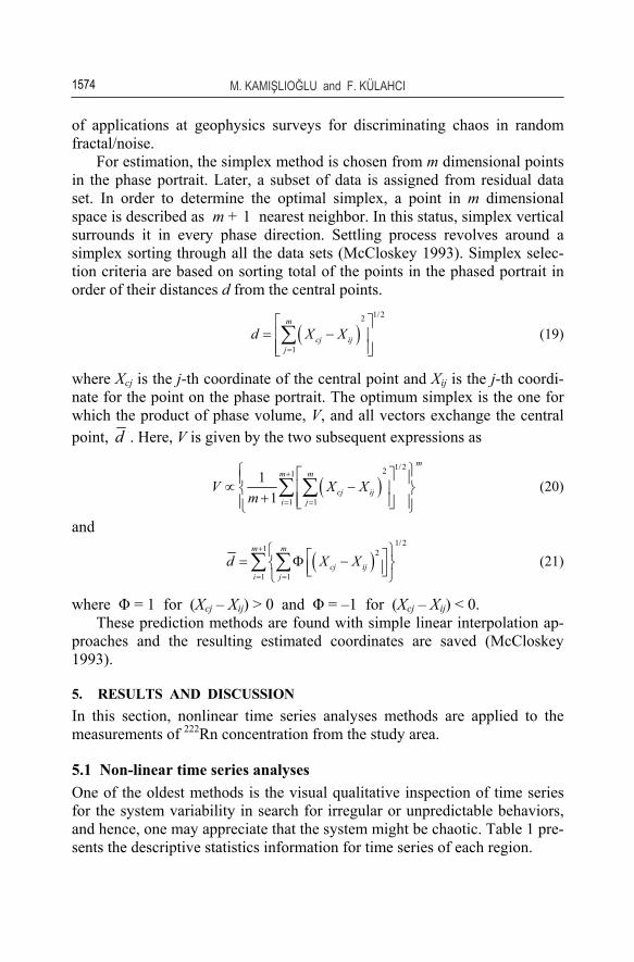
of applications at geophysics surveys for discriminating chaos in random fractal/noise.

For estimation, the simplex method is chosen from m dimensional points in the phase portrait. Later, a subset of data is assigned from residual data set. In order to determine the optimal simplex, a point in m dimensional space is described as m + 1 nearest neighbor. In this status, simplex vertical surrounds it in every phase direction. Settling process revolves around a simplex sorting through all the data sets (McCloskey 1993). Simplex selec-tion criteria are based on sorting total of the points in the phased portrait in order of their distances d from the central points.

( )1/22

1

m

cj ijj

d X X=

⎡ ⎤= −⎢ ⎥⎢ ⎥⎣ ⎦∑ (19)

where Xcj is the j-th coordinate of the central point and Xij is the j-th coordi-nate for the point on the phase portrait. The optimum simplex is the one for which the product of phase volume, V, and all vectors exchange the central point, d . Here, V is given by the two subsequent expressions as

( )1/ 221

1 1

11

mm m

cj iji j

V X Xm

+

= =

⎧ ⎫⎡ ⎤⎪ ⎪∝ −⎢ ⎥⎨ ⎬+ ⎢ ⎥⎪ ⎪⎣ ⎦⎩ ⎭∑ ∑ (20)

and

( )1/ 2

1 2

1 1

m m

cj iji j

d X X+

= =

⎧ ⎫⎡ ⎤= Φ −⎨ ⎬⎢ ⎥⎣ ⎦⎩ ⎭∑ ∑ (21)

where Φ = 1 for (Xcj – Xij) > 0 and Φ = –1 for (Xcj – Xij) < 0. These prediction methods are found with simple linear interpolation ap-

proaches and the resulting estimated coordinates are saved (McCloskey 1993).

5. RESULTS AND DISCUSSION In this section, nonlinear time series analyses methods are applied to the measurements of 222Rn concentration from the study area.

5.1 Non-linear time series analyses One of the oldest methods is the visual qualitative inspection of time series for the system variability in search for irregular or unpredictable behaviors, and hence, one may appreciate that the system might be chaotic. Table 1 pre-sents the descriptive statistics information for time series of each region.


1575

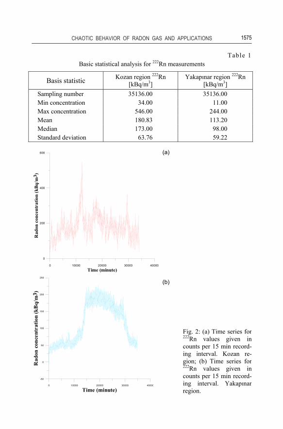
Table 1 Basic statistical analysis for 222Rn measurements

Basis statistic Kozan region 222Rn [kBq/m3]

Yakapınar region 222Rn [kBq/m3]

Sampling number 35136.00 35136.00 Min concentration 34.00 11.00 Max concentration 546.00 244.00 Mean 180.83 113.20 Median 173.00 98.00 Standard deviation 63.76 59.22

0 10000 20000 30000 40000

Time (minute)

0

200

400

600

Rad

onco

ncen

trat

ion

(kBq

/m3 )

0 10000 20000 30000 40000

Time (minute)

-50

0

50

100

150

200

250

Rad

on c

once

ntra

tion

(kB

q/m

3 )

(a)

(b)

Fig. 2: (a) Time series for 222Rn values given in counts per 15 min record-ing interval. Kozan re-gion; (b) Time series for 222Rn values given in counts per 15 min record-ing interval. Yakapınar region.


1576

Generally, standard statistical calculations do not give information about the system behavior. Figure 2 shows the observed 12 monthly data series for both regions (Kozan and Yakapınar). Altogether 35 136 measurements have the median, 173.00 kBq/m3, arithmetic average, 63.76 kBq/m3, and the standard deviation for Kozan. All data have the median of 98.00 kBq/m3; arithmetic average of 59.22 kBq/m3, and the standard deviation for Yakapınar (see Table 1). In order to use non-linear tools, data in Yakapınar region and time series should be stationary, for which FIR filter is applied by using the Kaiser window (see Fig. 2b).

Figure 2 presents the time series generated from one-year radon data. The genuine shape of time series obtained from 222Rn data is also given in the same figure, where there are periodic behaviors as an initial qualitative indicator of a possible chaotic behavior.

(a)

(b)

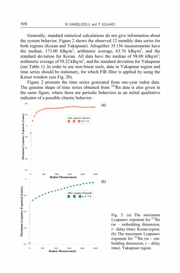
Fig. 3: (a) The maximum Lyapunov exponent for 222Rn (m – embedding dimension, τ – delay time). Kozan region; (b) The maximum Lyapunov exponent for 222Rn (m – em-bedding dimension, τ – delay time). Yakapınar region.

0 500 1000 1500 2000 2500

Radon Measurement

2.4

2.8

3.2

3.6

4

4.4

4.8

Max

imum

Lya

puno

vE

xpon

ent(

Lm

ax)

0 500 1000 1500 2000 2500

Radon Measurement

2.4

2.8

3.2

3.6

4

Max

imum

Lyap

unov

Exp

onen

t(Lm

ax)


1577

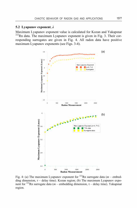
5.2 Lyapunov exponent, λ Maximum Lyapunov exponent value is calculated for Kozan and Yakapınar 222Rn data. The maximum Lyapunov exponent is given in Fig. 3. Their cor-responding surrogates are given in Fig. 4. All radon data have positive maximum Lyapunov exponents (see Figs. 3-4).

0 500 1000 1500 2000 2500

Radon Measurement

2.4

2.8

3.2

3.6

4

4.4

4.8

Max

imum

Lya

puno

vE

xpon

ent(

Lm

ax)

Max Lyapunov Exponentm=5, T=2Surrogates

0 500 1000 1500 2000 2500

Radon Measurement

2.4

2.8

3.2

3.6

4

Max

imum

Lyap

unov

Exp

onen

t(Lm

ax)

Fig. 4: (a) The maximum Lyapunov exponent for 222Rn surrogate data (m – embed-ding dimension, τ – delay time). Kozan region; (b) The maximum Lyapunov expo-nent for 222Rn surrogate data (m – embedding dimension, τ – delay time). Yakapınar region.

(a)

(b)


1578

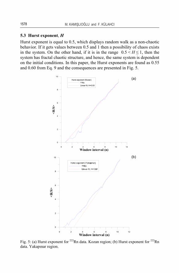
5.3 Hurst exponent, H Hurst exponent is equal to 0.5, which displays random walk as a non-chaotic behavior. If it gets values between 0.5 and 1 then a possibility of chaos exists in the system. On the other hand, if it is in the range 0.5 < H ≤ 1, then the system has fractal chaotic structure, and hence, the same system is dependent on the initial conditions. In this paper, the Hurst exponents are found as 0.55 and 0.60 from Eq. 9 and the consequences are presented in Fig. 5.

0 2 4 6 8 10 12

Window interval (n)

0

2

4

6

8

10

<R/S

>

Hurst exponent (Kozan)222RnLinear fit; H=0.55

0 2 4 6 8 10 12

Window interval (n)

0

2

4

6

8

10

<R/S

>

Fig. 5: (a) Hurst exponent for 222Rn data. Kozan region; (b) Hurst exponent for 222Rn data. Yakapınar region.

(a)

(b)


1579

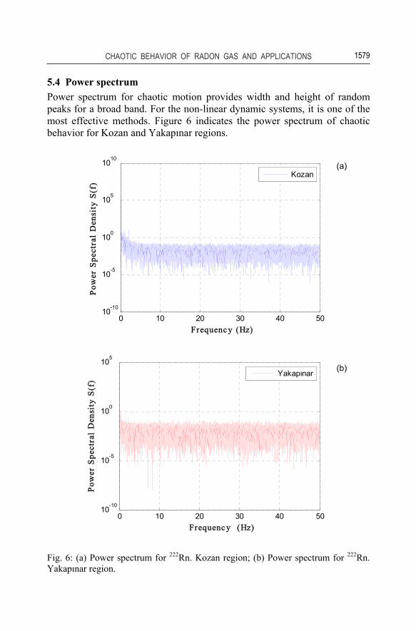
5.4 Power spectrum Power spectrum for chaotic motion provides width and height of random peaks for a broad band. For the non-linear dynamic systems, it is one of the most effective methods. Figure 6 indicates the power spectrum of chaotic behavior for Kozan and Yakapınar regions.

0 10 20 30 40 5010-10

10-5

100

105

1010

Frequenc y (Hz)

Pow

er S

pect

ral

Den

sity

S(f

)

Kozan

0 10 20 30 40 5010-10

10-5

100

105

Frequenc y (Hz)

Pow

er S

pect

ral

Den

sity

S(f

)

Yakapınar

Fig. 6: (a) Power spectrum for 222Rn. Kozan region; (b) Power spectrum for 222Rn. Yakapınar region.

(a)

(b)


1580

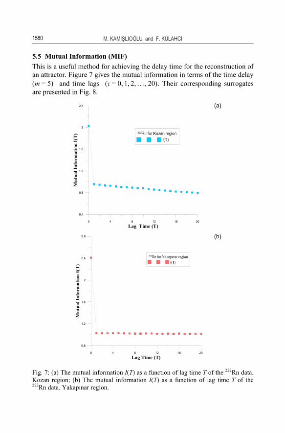
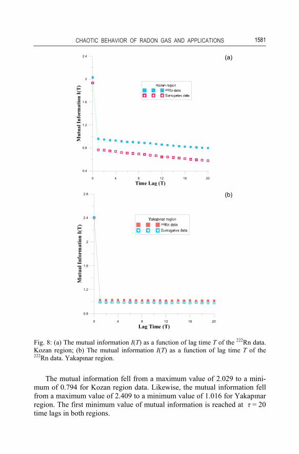
5.5 Mutual Information (MIF) This is a useful method for achieving the delay time for the reconstruction of an attractor. Figure 7 gives the mutual information in terms of the time delay (m = 5) and time lags (τ = 0, 1, 2, …, 20). Their corresponding surrogates are presented in Fig. 8.

0 4 8 12 16 20

Lag Time (T)

0.4

0.8

1.2

1.6

2

2.4

Mut

ualI

nfor

mat

ion

I(T)

0 4 8 12 16 20

Lag Time (T)

0.8

1.2

1.6

2

2.4

2.8

Mut

ualI

nfor

mat

ion

I(T)

Fig. 7: (a) The mutual information I(T) as a function of lag time T of the 222Rn data. Kozan region; (b) The mutual information I(T) as a function of lag time T of the 222Rn data. Yakapınar region.

(a)

(b)


1581

0 4 8 12 16 20

Time Lag (T)

0.4

0.8

1.2

1.6

2

2.4

Mut

ualI

nfor

mat

ion

I(T)

0 4 8 12 16 20

Lag Time (T)

0.8

1.2

1.6

2

2.4

2.8

Mut

ualI

nfor

mat

ion

I(T)

Fig. 8: (a) The mutual information I(T) as a function of lag time T of the 222Rn data. Kozan region; (b) The mutual information I(T) as a function of lag time T of the 222Rn data. Yakapınar region.

The mutual information fell from a maximum value of 2.029 to a mini-mum of 0.794 for Kozan region data. Likewise, the mutual information fell from a maximum value of 2.409 to a minimum value of 1.016 for Yakapınar region. The first minimum value of mutual information is reached at τ = 20 time lags in both regions.

(a)

(b)


1582

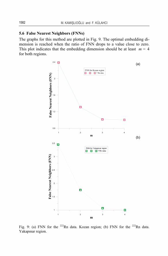
5.6 False Nearest Neighbors (FNNs) The graphs for this method are plotted in Fig. 9. The optimal embedding di-mension is reached when the ratio of FNN drops to a value close to zero. This plot indicates that the embedding dimension should be at least m = 4 for both regions.

1 2 3 4

m

0.8

1.2

1.6

2

2.4

False

Nea

rest

Nei

ghbo

rs(F

NN

)

FNN for Kozan region222Rn data

1 2 3 4

m

1

1.5

2

2.5

3

3.5

Fals

eN

eare

stN

eigh

bors

(FN

N)

FNN for Yakaplnar region222Rn data

Fig. 9: (a) FNN for the 222Rn data. Kozan region; (b) FNN for the 222Rn data. Yakapınar region.

(a)

(b)


1583

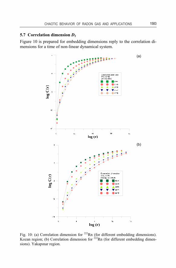
5.7 Correlation dimension D2 Figure 10 is prepared for embedding dimensions reply to the correlation di-mensions for a time of non-linear dynamical system.

Fig. 10: (a) Correlation dimension for 222Rn (for different embedding dimensions). Kozan region; (b) Correlation dimension for 222Rn (for different embedding dimen-sions). Yakapınar region.

(a)

(b)


1584

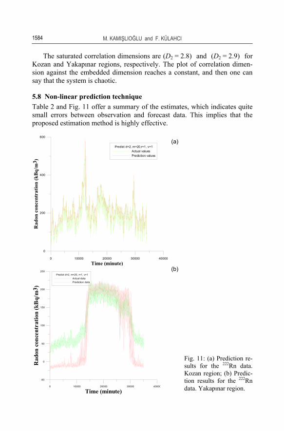
The saturated correlation dimensions are (D2 = 2.8) and (D2 = 2.9) for Kozan and Yakapınar regions, respectively. The plot of correlation dimen-sion against the embedded dimension reaches a constant, and then one can say that the system is chaotic.

5.8 Non-linear prediction technique Table 2 and Fig. 11 offer a summary of the estimates, which indicates quite small errors between observation and forecast data. This implies that the proposed estimation method is highly effective.

0 10000 20000 30000 40000

Time (minute)

0

200

400

600

Rad

onco

ncen

trat

ion

(kBq

/m3 )

Predict d=2, m=20,r=1, v=1Actual valuesPrediction values

0 10000 20000 30000 40000

Time (minute)

-50

0

50

100

150

200

250

Rad

on c

once

ntra

tion

(kB

q/m

3 )

Predict d=2, m=20, r=1, v=1Actual dataPrediction data

(a)

(b)

Fig. 11: (a) Prediction re-sults for the 222Rn data. Kozan region; (b) Predic-tion results for the 222Rn data. Yakapınar region.


1585

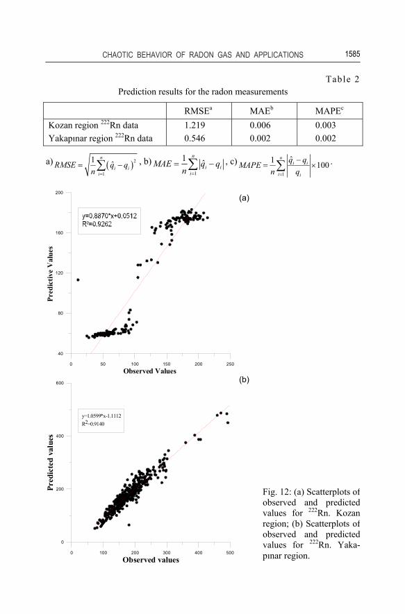
Table 2 Prediction results for the radon measurements

RMSEa MAEb MAPEc

Kozan region 222Rn data 1.219 0.006 0.003 Yakapınar region 222Rn data 0.546 0.002 0.002

a) ( )2

1

1 ˆn

i ii

RMSE q qn =

= −∑ , b)1

1 ˆn

i ii

MAE q qn =

= −∑ , c)1

ˆ1 100n

i i

i i

q qMAPEn q=

−= ×∑ .

0 50 100 150 200 250

Observed Values

40

80

120

160

200

Pred

ictiv

eV

alue

s

0 100 200 300 400 500

Observed values

0

200

400

600

Pred

icte

dva

lues

y=1.0599*x-1.1112R2=0.9140

(a)

(b)

Fig. 12: (a) Scatterplots of observed and predicted values for 222Rn. Kozanregion; (b) Scatterplots of observed and predicted values for 222Rn. Yaka-pınar region.


1586

Scatter plots of observed and predicted 222Rn concentration values are given in Fig. 12. It is clear that the results give accurate predictions. General-ly, they show the noticeable performance of chaos theory in estimating the future states of large scale dynamic systems. Figure 12 also shows the rela-tion between observed and predicted 222Rn concentration values with R2 for Kozan to and Yakapınar regions as 0.926 and 0.9140, respectively. The rela-tion between the observed and predicted concentrations can be estimated with non-linear predicted methods.

6. CONCLUSIONS In this paper, chaotic behavior of soil radon gas has been searched through a set of nonlinear analyses techniques for the data recorded. The non-linear prediction methods are applied for prediction of the 222Rn concentration for Kozan and Yakapınar regions near East Anatolian Fault System (EAFS) in Turkey. Nonlinear time series analyses are performed to understand the propagation of 222Rn concentration in the soil. Preliminary analysis confirms the chaotic structure of the data sets in this paper.

In this research, nonlinear analysis of the soil 222Rn concentration are presented and discussed through the chaotic behavior approaches. The non-linear analysis of time series with various tools is a powerful tool to under-stand the chaotic dynamics in complex systems. Lyapunov exponent and fractal correlation dimension give information about a dynamical system chaotic behavior. The broadband power spectrum proofs with clear dominant frequency that it is in a chaotic structure of 222Rn data. Surrogate data meth-od is used for verifying the existence of low-dimensional chaos; this method is based on a statistical approach for determining the non-linearity in time series. Conclusions indicate that the given time series can be distinguished from noise of 222Rn data. The mathematical and physical meanings of this expression are based on a high-dimensional chaotic structure. To observe this chaotic behavior, it must reach saturation correlation dimension of dy-namic system. In this study, it is concluded that chaotic behavior of dynamic system reaches saturation. The first minimum point value of mutual infor-mation function is determined as delay time. Especially, the mutual infor-mation function indicates slim correlations regarding the intervention time.

The conclusion of chaotic time series analyses shows the reflection of the chaotic behavior of the complex dynamic systems concerning radon em-anation and transport in natural sub-surface systems. The results obtained show robust chaos signature of the radon time series. One can say that the er-rors between the observation and the prediction are very small, which sug-gests that prediction is very effective. It is clear from the scatterplots that the results give reliable predictions when compared with raw data.


1587

Acknowledgemen t s . This work was supported by TUBITAK 2211-C Priority Areas Related to Doctoral Scholarship Program and Republic of Turkey Prime Ministry Disaster & Emergency Management Presidency (AFAD).

R e f e r e n c e s

Abarbanel, H.D.I., R. Brown, J.J. Sidorowich, and L.S. Tsimring (1993), The analy-sis of observed chaotic data in physical systems, Rev. Mod. Phys. 65, 4, 1331-1392, DOI: 10.1103/RevModPhys.65.1331.

Albarello, D., V. Lapenna, G. Martinelli, and L. Telesca (2003), Extracting quantita-tive dynamics from 222Rn gaseous emissions of mud volcanoes, Environ-metrics 14, 1, 63-71, DOI: 10.1002/env.565.

Alvarez-Ramirez, J., J. Alvarez, E. Rodriguez, and G. Fernandez-Anaya (2008), Time-varying hurst exponent for US stock markets, Physica A 387, 24, 6159-6169, DOI: 10.1016/j.physa.2008.06.056.

Bak, P., C. Tang, and K. Wiesenfeld (1988), Self-organized critically, Phys. Rev. A 38, 1, 364-374, DOI: 10.1103/PhysRevA.38.364.

Bourai, A.A., S. Aswal., A. Dangwal, M. Rawat, M. Prasad, N.P. Naithani, V. Joshi, and R.C. Ramola (2013), Measurements of radon flux and soil-gas radon concentration along the Main Central Thrust, Garhwal Himalaya, using SRM and RAD7 detectors, Acta Geophys. 61, 4, 950-957, DOI: 10.2478/ s11600-013-0132-2.

Chaudhuri, H., C. Barman, A.N.S. Iyengar, D. Ghose, P. Sen, and B. Sinha (2013), Network of seismo-geochemical monitoring observatories for earthquake prediction research in India, Acta Geophys. 61, 4, 1000-1025, DOI: 10.2478/s11600-013-0134-0.

Chouet, B., and H.R. Shaw (1991), Fractal properties of temor and gas piston events observed at Kilauea Volcano Hawaii, J. Geophys. Res. 96, B6, 10177-10189, DOI: 10.1029/91JB00772.

Chyi, L.L., T.J. Quick, T.F. Yang, and C.H. Chen (2010), The experimental investi-gation of soil gas radon migration mechanisms and its implication in earth-quake forecast, Geofluids 10, 4, 556-563, DOI: 10.1111/j.1468-8123.2010. 00308.x.

Cothern, C.R., and J.E. Smith (1987). Environmental Radon, Environmental Science Research, Vol. 35, Plenum Press, New York.

Crisanti, A., M.H., Jensen, A. Vulpiani, and G. Paladin (1992), Strongly intermittent chaos and scaling in an earthquake model, Phys. Rev. Lett. 46, 12, 7363-7366, DOI: 10.1103/PhysRevA.46.R7363.


1588

Cuculeanu, V., and A. Lupu (1996), Fractal dimensions of the outdoor radon iso-topes time series, Environ. Int. 22, 1, 171-179, DOI: 10.1016/S0160-4120(96)00105-5.

Das, N.K., P. Sen, R.K. Bhandari, and B. Sinha (2009), Nonlinear response of radon and its progeny in spring emission, Appl. Radiat. Isotopes 67, 2, 313-318, DOI: 10.1016/j.apradiso.2008.09.016.

Durrani, S.A., and R. Ilić (eds.) (1997), Radon Measurements by Etched Track De-tectors. Applications in Radiation Protection, Earth Sciences and the Envi-ronment, World Scientific Publ. Co. Pte. Ltd, Signapore.

Eckhardt, B., and D. Yao (1993), Local Lyapunov exponents in chaotic systems, Physica D 65, 1-2, 100-108, DOI: 10.1016/0167-2789(93)90007-N.

Eckmann, J.P., and D. Ruelle (1985), Ergodic theory of chaos and strange attractors, Rev. Mod. Phys. 57, 3, 617-656, DOI: 10.1103/RevModPhys.57.617.

Feller, W. (1951), The asymptotic distribution of the range of sums of independent random variables. Ann. Math Stat. 22, 3, 427-443, DOI: 10.1214/aoms/ 1177729589.

Fleischer, R.L. (1981), Discolation model for radon response to distant earthquakes, Geophys. Res. Lett. 8, 5, 477-480, DOI: 10.1029/GL008i005p00477.

Fleischer, R.L., and A. Magro-Campero (1985), Association of subsurface radon changes in Alaska and the northeastern United States with earthquakes, Geochim. Cosmochim, Ac. 49, 4, 1061-1071, DOI: 10.1016/0016-7037(85) 90319-9.

Fraser, A.M., and H.L. Swinney (1986), Independent coordinates for strange attrac-tors from mutual information, Phys. Rev. A 33, 2, 1134-1140, DOI: 10.1103/PhysRevA.33.1134.

Frazier, C., and K.M. Kockelman (2004), Chaos theory and transportation systems: an instructive, J. Transport. Res. Board. 1897, 9-17, DOI: 10.3141/1897-02.

Friedmann, H., K. Aric, R. Gutdeutsch, C.Y. King, C. Altay, and H. Sav (1988), Ra-don measurements for earthquake prediction along the North Anatolian zone: a progress report, Tectonophysics 152, 3-4, 209-214, DOI: 10.1016/ 0040-1951(88)90047-9.

Ghosh, D., A. Deb, R. Sengupta, K. Patra, and S. Bera (2007), Pronounced soil-radon anomaly-precursor of recent earthquakes in India, Radiat. Meas. 42, 3, 466-471, DOI: 10.1016/j.radmeas.2006.12.008.

Grassberger, P., and I. Procaccia (1983), Characterization of strange attractors, Phys. Rev. Lett. 50, 5, 346-349, DOI: 10.1103/PhysRevLett.50.346.

Gutenberg, B., and C.F. Richter (1954), Seismicity of the Earth and Associated Phe-nomena, Princeton University Press, Princeton, NJ.

Harris, C.M., R.W. Todd, S.J. Bungard, R.W. Lovitt, J.G. Morris, and D.B. Kell (1987), The dielectric permittivity of microbial suspensions at radio-


1589

frequencies: a novel method for estimation of microbial biomass, Enzyme Microb. Tech. 9, 3, 181-186, DOI: 10.1016/0141-0229(87)90075-5.

Hurst, H.E. (1951), Long-term storage capacity of reservoirs, Trans. Am. Soc. Civil. Eng. 116, 770-808.

Igarashi, G., and S. Saeki (1995), Groundwater radon anomaly before the Kobe earthquake in Japan, Science 269, 5220, 60-61, DOI: 10.1126/science.269. 5220.60.

Kamışlıoğlu, M., F. Külahcı, and F. Özkaynak (2013), Nonlinear reply of soil radon (222Rn) gas measurements and deterministic chaos, Chaotic Model. Simul. (CMSIM) 2, 153-160.

Kaplan, J., and J. Yorke (1979), Functional Differential Equations and the Ap-proximation of Fixed Points, Lecture Notes in Mathematics, No. 730, Springer Verlag, Berlin.

Karig, D.E., and H. Kozlu (1990), Late Paleogene-Neogene evolution of the triple junction region near Maraş, south-central Turkey, J. Geol. Soc. 147, 6, 1023-1034, DOI: 10.1144/gsjgs.147.6.1023.

Kennel, M.B., R. Brown, and H.D.I. Abarbanel (1992), Determining embedding di-mension for phase-space reconstruction using a geometrical construction, Phys. Rev. A 45, 6, 3403-3411, DOI: 10.1103/PhysRevA.45.3403.

Khatibi, R., B. Sivakumar, M.A. Ghorbani, O. Kisi, K. Kocak, and D. Farshidizadeh (2012), Investigating chaos in river stage and discharge time series, J. Hy-drol. 414, 108-117, DOI: 10.1016/j.jhydrol.2011.10.026.

King, C.Y. (1986), Gas geochemistry applied to earthquake prediction: an overview, J. Geophys. Res. 91, B12, 2269-2281, DOI: 10.1029/JB091iB12p12269.

King, C.Y., W. Zhang, and B.S. King (1993), Radon anomalies on three kind of faults in California, Pure Appl. Geophys. 141, 1, 111-124, DOI: 10.1007/ BF00876238.

Koçak, K., and Z. Şen (1998), More information regarding dynamical systems via convergence to correlation dimension, Interdiscipl. J. Phys. Eng. Sci. 51, 1, 1-5, DOI: 10.1007/s007770050022.

Külahcı, F., and Z. Şen (2014), On the correction of spatial and statistical uncertain-ties in systematic measurements of 222Rn for earthquake prediction, Surv. Geophys. 35, 2, 449-478, DOI: 10.1007/s10712-013-9273-8.

Külahcı, F., M. İnceöz, M. Doğru, E. Aksoy, and O. Baykara (2009), Artifical neural network model for earthquake prediction with radon monitoring, Appl. Ra-diat. Isotopes 67, 1, 212-219, DOI: 10.1016/j.apradiso.2008.08.003.

Kumar, A., V. Walia, T.F. Yang, H.H. Chang, S.J. Lin, K.P. Eappen, and B.R. Arora (2013), Radon-thoron monitoring in Tatun volcanic areas of northern Tai-wan using LR-115 alpha track detector technique: Pre-calibration and in-stallation, Acta Geophys. 61, 4, 958-976, DOI: 10.2478/s11600-013- 0120-6.


1590

Kumar, N., G. Rawat., V.M. Choubey., and D. Hazarika (2013), Earthquake precur-sory research in western Himalaya based on the multi-parametric geophysi-cal observatory data, Acta Geophys. 61, 4, 977-999, DOI: 10.2478/s11600-013-0133-1.

Lakshmi, S.S., and R.K. Tiwari (2009), Model dissection from earthquake time se-ries: A comparative analysis using modern non-linear forecasting and artifi-cial neural network approaches, Computat. Geosci. 35, 2,191-204, DOI: 10.1016/j.cageo.2007.11.011.

Lane-Smith, D., and K.W.W. Sims (2013), The effect of CO2 on the measurement of Rn-220 and Rn-222 with instruments utilising electrostatic precipitation, Acta Geophys. 61, 4, 822-830, DOI: 10.2478/s11600-013-0107-3.

Martinelli, G. (2015), Hydrogeologic and geochemical precursor of earthquakes: an assesment for possible applications, Boll. Geof. Teor. Appl. 56, 2, 83-94.

McCloskey, J. (1993), A hierarchical model for earthquake generation on coupled segments of a transform fault, Geophys. J. Int. 115, 2, 538-551, DOI: 10.1111/j.1365-246X.1993.tb01205.x.

Miklavčić, I., B. Radolić, M. Vuković, M. Poje, M. Varga, D. Stanić, and J. Planinić (2008), Radon anomaly in soil gas an earthquake precursor, Appl. Radiat. Isotopes 66, 10, 1459-1466, DOI: 10.1016/j.apradiso.2008.03.002.

Namvaran, M., and A. Negarestani (2015), Noise reduction in radon monitoring data using Kalman filter and application of results in earthquake precursory process research, Acta Geophys. 63, 2, 329-351, DOI: 10.2478/s11600-014-0218-5.

Planinić, J., B. Vuković, and V. Radolić (2004), Radon time variations and determi-nistic chaos, J. Environ. Radioactiv. 75, 1, 35-45, DOI: 10.1016/j.jenvrad. 2003.10.007.

Provenzale, A., L.A. Smith, R. Vio, and G. Murante (1992), Distinguishing between low-dimensional dynamics and randomness in measured time series, Physica D 1-4, 58, 31-49, DOI: 10.1016/0167-2789(92)90100-2.

Qiang, L., and X. Gui-Ming (2012), Characteristic variation of local scaling property before Puer M6.4 earthquake in China: The presence of a new pattern of nonlinear behavior of seismicity, Izv. Phys. Solid Earth 48, 2, 155-161, DOI: 10.1134/S1069351312010107.

Sakata, S., J. Hayano, S. Mukai, A. Okada, B. Galdrikian, and J.D. Farmeret (1999), Aging and spectral characteristic of the nonharmonic component of 24-h heart rate variability, Am. J. Physiol.–Reg. 276, 1724-1731.

Sano, M., and Y. Sawada (1985), Measurement of the Lyapunov spectrum from a chaotic time series, Phys. Rev. Lett. 55, 10, 1082-1085, DOI: 10.1103/ PhysRevLett.55.1082.

Sato, S., M. Sano, and Y. Sawada (1987), Practical methods of measuring the gener-alized dimension and the largest Lyapunov exponent in high dimensional chaotic systems, Prog. Theor. Phys. 77, 1, 1-5, DOI: 10.1143/PTP.77.1.


1591

Şen, Z. (1977a), Small sample estimation of h, Water Resour. Res. 13, 6, 971-974, DOI: 10.1029/WR013i006p00971.

Şen, Z. (1977b), Small sample expectation of population and adjusted ranges, Water Resour Res. 13, 6, 975-980, DOI: 10.1029/WR013i006p00975.

Şen, Z. (1977c), Small sample expectation of rescaled population and rescaled ad-justed ranges, Water Resour. Res. 13, 6, 981-986, DOI: 10.1029/ WR013i006p00981.

Smirnov, V.B., A.V. Ponomarev, Q. Jiadongand, and A.S. Cherepantsev (2005), Rhythms and deterministic chaos in geophysical time series, Izv. Phys. Solid Earth 41, 6, 428-448.

Smith, L.A., J.D. Fournier, and E.A. Spiegel (1986), Lacunarity and intermittency in fluid turbulence, Phys. Lett. A 114, 8-9, 465-468, DOI: 10.1016/0375-9601(86)90695-X.

Sprott, J (2003), Chaos and Time-Series Analysis, Oxford University Press, New York.

Sugihara, G., and R.M. May (1990), Nonlinear forecasting as a way of distinguish-ing chaos from measurement error in time series, Nature 344, 6268, 734-741, DOI: 10.1038/344734a0.

Takens, F. (1981), Detecting strange attractors in turbulence. In: Dynamical Systems and Turbulence, Warwick 1980, Lecture Notes in Mathematics, Vol. 898, Springer, Berlin, Heidelberg, 366-381, DOI: 10.1007/BFb0091924.

Tarakçı, M., C. Harmanşah, M.M. Saç, and M. İçhedef (2014), Investigation of the relationships between seismic activities and radon level in Western Turkey, Appl. Radiat. Isotopes 83A, 12-17, DOI: 10.1016/j.apradiso.2013.10.008.

Theiler, J. (1988), Lacunarity in a best estimator of fractal dimension, Phys. Lett. A 133, 4-5, 195-200, DOI: 10.1016/0375-9601(88)91016-X.

Theiler, J. (1991), Some comments on the correlation dimension of 1/fα noise, Phys. Lett. A 155, 8-9, 480-493, DOI: 10.1016/0375-9601(91)90651-N.

Theiler, J., S. Eubank, A. Longtin, B. Galdrikian, and J.D. Farmer (1992), Testing for nonlinearity in time series: the method of surrogate data, Physica D 58, 1-4, 77-94, DOI: 10.1016/0167-2789(92)90102-S.

Tiwari, R.K., S.S. Lakshmi, and K.N.N. Rao (2004), Characterization of earthquake dynamics in northeastern India regions: A modern nonlinear forecasting approach, Pure. Appl. Geophys. 161, 4, 865-880, DOI: 10.1007/s00024-003-2476-z.

Ulomov, V.I., and B.Z. Mavashev (1967), A precursor of strong tectonic earthquake, Dokl. Acad. Sci. USSR Earth Sci. Sect. 176, 9-11.

Wakita, H., G. Igarashi, and K. Notsu (1991), An anomalous radon decrease in groundwater prior to an M6.0 Earthquake: A Possible Precursor? Geophys. Res. Lett. 18, 4, 629-632, DOI: 10.1029/91GL00824.

Woith, H. (2015), Radon earthquake precursor: A short review, Eur. Phys. J. Spec. Top. 224, 4, 611-627, DOI: 10.1140/epjst/e2015-02395-9.


1592

Wolf, A. (1985), Determining Lyapunov exponents from a time series, Physica D 16, 3, 285-317, DOI: 10.1016/0167-2789(85)90011-9.

Received 2 September 2015 Received in revised form 26 January 2016

Accepted 29 January 2016

chaotic behavior of soil radon gas and...

Documents