channel estimation and symbol detection in massive mimo
TRANSCRIPT
Louisiana State UniversityLSU Digital Commons
LSU Doctoral Dissertations Graduate School
2017
Channel Estimation and Symbol Detection InMassive MIMO Systems Using ExpectationPropagationKamran GhavamiLouisiana State University and Agricultural and Mechanical College, [email protected]
Follow this and additional works at: https://digitalcommons.lsu.edu/gradschool_dissertations
Part of the Electrical and Computer Engineering Commons
This Dissertation is brought to you for free and open access by the Graduate School at LSU Digital Commons. It has been accepted for inclusion inLSU Doctoral Dissertations by an authorized graduate school editor of LSU Digital Commons. For more information, please [email protected].
Recommended CitationGhavami, Kamran, "Channel Estimation and Symbol Detection In Massive MIMO Systems Using Expectation Propagation" (2017).LSU Doctoral Dissertations. 4378.https://digitalcommons.lsu.edu/gradschool_dissertations/4378
CHANNEL ESTIMATION AND SYMBOL DETECTION IN MASSIVE MIMOSYSTEMS USING EXPECTATION PROPAGATION
A Dissertation
Submitted to the Graduate Faculty of theLouisiana State University and
Agricultural and Mechanical Collegein partial fulfillment of the
requirements for the degree ofDoctor of Philosophy
in
The School of Electrical Engineering and Computer Sciences
byKamran Ghavami
B.S., University of Tehran, 1998M.S., University of Tehran, 2001
August 2017

To Aram, Janan, and Hafez
ii

AcknowledgmentsFirst and foremost, I would like to express my sincere appreciation to my advisor, Prof.
Morteza Naraghi-Pour, for the professional academic guidance he provided to me, and his
patience, confidence and care throughout these years. This dissertation would not have
been accomplished without his generous support and valuable suggestions.
Also, I would like to express my gratitude to my doctoral committees, Dr. Xuebin
Liang, and Dr. Shuangqing Wei for their kind support and thoughtful comments.
I would thank my wife, Aram, who have been always encouraging and supporting me
since the early steps toward my doctoral degree.
iii
Table of ContentsDEDICATION . . . . . . . . . . . . . . . . . . . . . . . . . . . . . . . . . . . . . . . . . . . . . . . . . . . . . . . . . . . . . . . . . . . ii
ACKNOWLEDGMENTS . . . . . . . . . . . . . . . . . . . . . . . . . . . . . . . . . . . . . . . . . . . . . . . . . . . . . . . . . iii
LIST OF TABLES . . . . . . . . . . . . . . . . . . . . . . . . . . . . . . . . . . . . . . . . . . . . . . . . . . . . . . . . . . . . . . . vi
LIST OF FIGURES . . . . . . . . . . . . . . . . . . . . . . . . . . . . . . . . . . . . . . . . . . . . . . . . . . . . . . . . . . . . . . vii
ABSTRACT . . . . . . . . . . . . . . . . . . . . . . . . . . . . . . . . . . . . . . . . . . . . . . . . . . . . . . . . . . . . . . . . . . . . . . x
CHAPTER1 INTRODUCTION . . . . . . . . . . . . . . . . . . . . . . . . . . . . . . . . . . . . . . . . . . . . . . . . . . . . . . . . . 1
1.1 Massive MIMO . . . . . . . . . . . . . . . . . . . . . . . . . . . . . . . . . . . . . . . . . . . . . . . . . . . . . . . 21.2 Challenges in Channel Estimation in Massive MIMO Systems. . . . . . . . . . 71.3 Challenges in Symbol Detection in Massive MIMO Systems . . . . . . . . . . . . 111.4 Outline of the Dissertation . . . . . . . . . . . . . . . . . . . . . . . . . . . . . . . . . . . . . . . . . . . . 12
2 MIMO DETECTIONWITH IMPERFECT CHANNEL STATEINFORMATION USING EXPECTATION PROPAGATION. . . . . . . . . . . . . . . . 142.1 Introduction . . . . . . . . . . . . . . . . . . . . . . . . . . . . . . . . . . . . . . . . . . . . . . . . . . . . . . . . . . 142.2 System Model . . . . . . . . . . . . . . . . . . . . . . . . . . . . . . . . . . . . . . . . . . . . . . . . . . . . . . . . 172.3 Expectation Propagation . . . . . . . . . . . . . . . . . . . . . . . . . . . . . . . . . . . . . . . . . . . . . 182.4 EP algorithm for imperfect CSI . . . . . . . . . . . . . . . . . . . . . . . . . . . . . . . . . . . . . . . 21
2.4.1 Motivation . . . . . . . . . . . . . . . . . . . . . . . . . . . . . . . . . . . . . . . . . . . . . . . . . . 212.4.2 Channel estimation . . . . . . . . . . . . . . . . . . . . . . . . . . . . . . . . . . . . . . . . . . 232.4.3 EP formulation for correlated noise channel . . . . . . . . . . . . . . . . . . 26
2.5 Simulation Results and Observations . . . . . . . . . . . . . . . . . . . . . . . . . . . . . . . . . . 292.5.1 Simulation setup . . . . . . . . . . . . . . . . . . . . . . . . . . . . . . . . . . . . . . . . . . . . 292.5.2 Numerical results . . . . . . . . . . . . . . . . . . . . . . . . . . . . . . . . . . . . . . . . . . . . 31
3 NONCOHERENT SIMO DETECTION BY EXPECTATIONPROPAGATION . . . . . . . . . . . . . . . . . . . . . . . . . . . . . . . . . . . . . . . . . . . . . . . . . . . . . . . . . . 383.1 Introduction . . . . . . . . . . . . . . . . . . . . . . . . . . . . . . . . . . . . . . . . . . . . . . . . . . . . . . . . . . 383.2 System Model . . . . . . . . . . . . . . . . . . . . . . . . . . . . . . . . . . . . . . . . . . . . . . . . . . . . . . . . 403.3 EP formulation for noncoherent detection . . . . . . . . . . . . . . . . . . . . . . . . . . . . . 423.4 Numerical Results . . . . . . . . . . . . . . . . . . . . . . . . . . . . . . . . . . . . . . . . . . . . . . . . . . . . 49
4 JOINT CHANNEL ESTIMATION AND SYMBOL DETEC-TION FOR MULTI-CELL MASSIVE MIMO USING EX-PECTATION PROPAGATION . . . . . . . . . . . . . . . . . . . . . . . . . . . . . . . . . . . . . . . . . . . . 544.1 Introduction . . . . . . . . . . . . . . . . . . . . . . . . . . . . . . . . . . . . . . . . . . . . . . . . . . . . . . . . . . 544.2 System Model . . . . . . . . . . . . . . . . . . . . . . . . . . . . . . . . . . . . . . . . . . . . . . . . . . . . . . . . 584.3 Review of the EVD-Based Massive MIMO Channel Estimation . . . . . . . . 624.4 EP Formulation for Noncoherent Detection . . . . . . . . . . . . . . . . . . . . . . . . . . . . 65
iv

4.4.1 Calculation of qnew(h) and updating of qt(h) . . . . . . . . . . . . . . . . . 684.4.2 Calculation of qnew(S) and updating of qt(st) . . . . . . . . . . . . . . . . . 704.4.3 A Low-Complexity Approximation . . . . . . . . . . . . . . . . . . . . . . . . . . . 72
4.5 Numerical Results . . . . . . . . . . . . . . . . . . . . . . . . . . . . . . . . . . . . . . . . . . . . . . . . . . . . 74
5 CONCLUSION . . . . . . . . . . . . . . . . . . . . . . . . . . . . . . . . . . . . . . . . . . . . . . . . . . . . . . . . . . . . 81
REFERENCES . . . . . . . . . . . . . . . . . . . . . . . . . . . . . . . . . . . . . . . . . . . . . . . . . . . . . . . . . . . . . . . . . . . . 83
APPENDIXA STATISTICAL INFERENCE BY MESSAGE PASSING . . . . . . . . . . . . . . . . . . . . 88
A.1 Graphical Structures. . . . . . . . . . . . . . . . . . . . . . . . . . . . . . . . . . . . . . . . . . . . . . . . . . 88A.2 Sum-Product Algorithm . . . . . . . . . . . . . . . . . . . . . . . . . . . . . . . . . . . . . . . . . . . . . . 90A.3 Applications of the BP Algorithm in MIMO Detection . . . . . . . . . . . . . . . . . 92
B PROPERTIES OF GAUSSIN RANDOM VECTORS . . . . . . . . . . . . . . . . . . . . . . . 97
C ASSUMED DENSITY FILTERING . . . . . . . . . . . . . . . . . . . . . . . . . . . . . . . . . . . . . . . . 98
D PROOF OF THE MOMENT MATCHING PROPERTY . . . . . . . . . . . . . . . . . . . 100
E ADF EQUATIONS FOR GAUSSIAN RANDOM VECTORS . . . . . . . . . . . . . . . 102
F CALCULATING ZT . . . . . . . . . . . . . . . . . . . . . . . . . . . . . . . . . . . . . . . . . . . . . . . . . . . . . . . 106
G HYBRID K-L DIVERGENCE OPTIMIZATION PROBLEM . . . . . . . . . . . . . . . 107
VITA . . . . . . . . . . . . . . . . . . . . . . . . . . . . . . . . . . . . . . . . . . . . . . . . . . . . . . . . . . . . . . . . . . . . . . . . . . . . . 110
v

List of Tables1.1 Examples of open-loop and closed-loop MIMO systems. . . . . . . . . . . . . . . . . . . . . . . 2
4.1 The percentage of the erroneous detected frames. . . . . . . . . . . . . . . . . . . . . . . . . . . . . 77
vi
List of Figures1.1 An implemented massive MIMO BS with 160 dual-polarized
patch antennas [1]. . . . . . . . . . . . . . . . . . . . . . . . . . . . . . . . . . . . . . . . . . . . . . . . . . . . . . . . . . . 3
1.2 Network model in massive MIMO. . . . . . . . . . . . . . . . . . . . . . . . . . . . . . . . . . . . . . . . . . . . 4
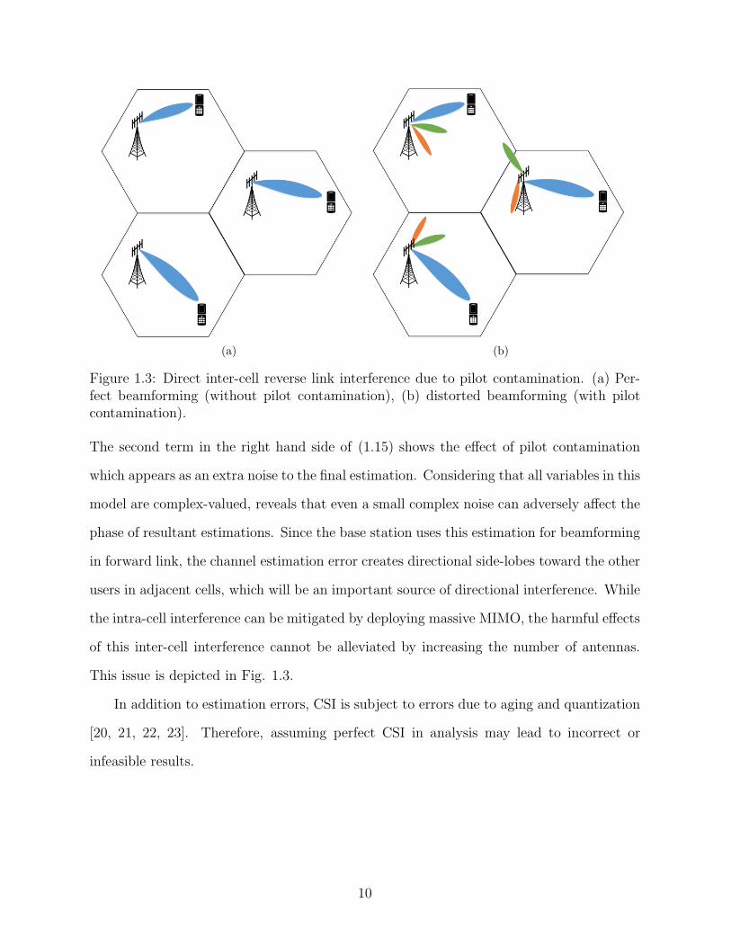
1.3 Direct inter-cell reverse link interference due to pilot contami-nation. (a) Perfect beamforming (without pilot contamination),(b) distorted beamforming (with pilot contamination). . . . . . . . . . . . . . . . . . . . . . . . 10
2.1 Decoding performance of the EP decoder and the channel es-timation error for 12 × 12 antenna configuration and 16-QAMmodulation. . . . . . . . . . . . . . . . . . . . . . . . . . . . . . . . . . . . . . . . . . . . . . . . . . . . . . . . . . . . . . . . . . 22
2.2 Decoding performance of MMSE and EP decoders versus thechannel estimation mean square error for 20× 20 antenna con-figuration and 16-QAM modulation. . . . . . . . . . . . . . . . . . . . . . . . . . . . . . . . . . . . . . . . . . 22
2.3 The search regions for the EP and Modified EP algorithms. (a)EP with uncorrelated covariance, and (b) Modified EP with cor-related covariance. . . . . . . . . . . . . . . . . . . . . . . . . . . . . . . . . . . . . . . . . . . . . . . . . . . . . . . . . . . 24
2.4 Detection performance for the MIMO system with 16-QAMmod-ulation and orthogonal pilot vectors with Nr = Nt = 32 anduncorrelated MIMO channel. . . . . . . . . . . . . . . . . . . . . . . . . . . . . . . . . . . . . . . . . . . . . . . . . 31
2.5 Detection performance for the MIMO system with 16-QAMmod-ulation and orthogonal pilot vectors with Nr = Nt = 64 anduncorrelated MIMO channel.. . . . . . . . . . . . . . . . . . . . . . . . . . . . . . . . . . . . . . . . . . . . . . . . . 32
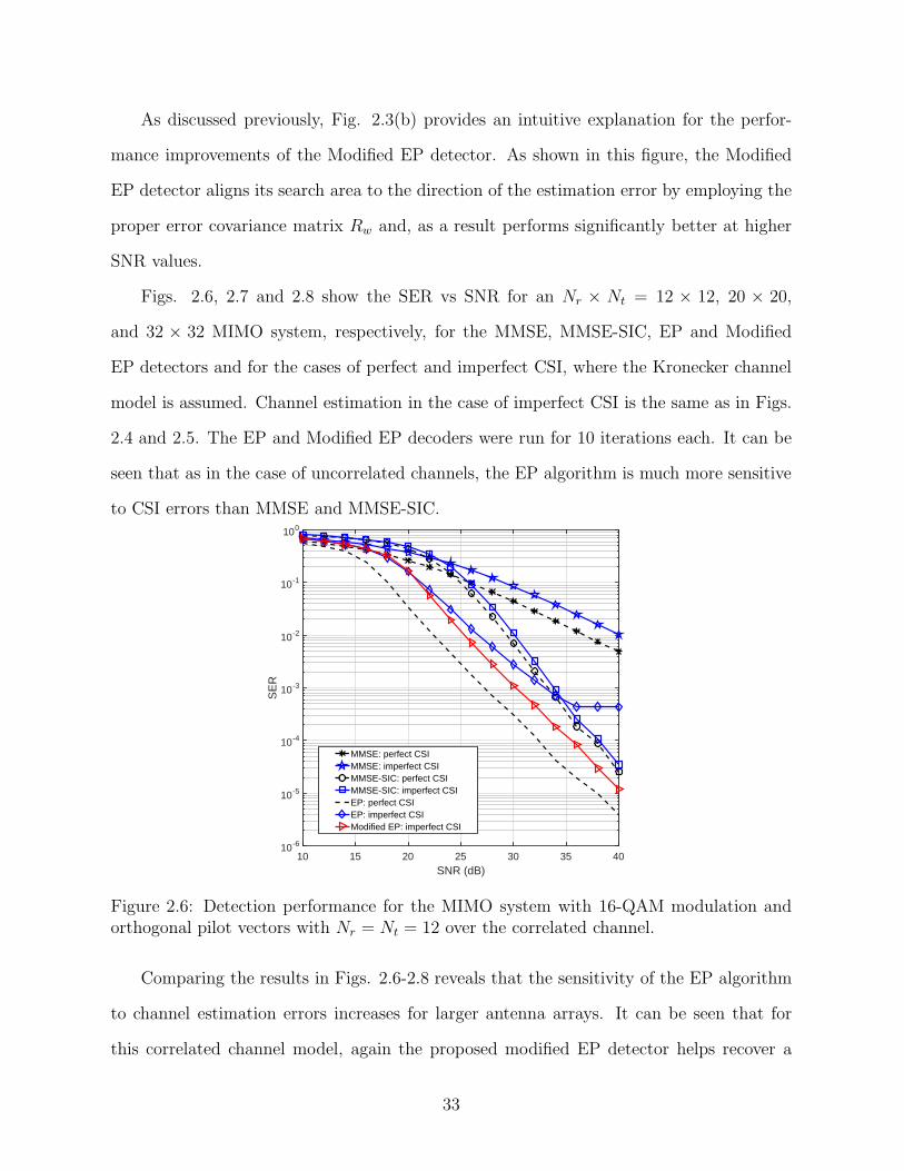
2.6 Detection performance for the MIMO system with 16-QAMmod-ulation and orthogonal pilot vectors with Nr = Nt = 12 over thecorrelated channel. . . . . . . . . . . . . . . . . . . . . . . . . . . . . . . . . . . . . . . . . . . . . . . . . . . . . . . . . . . 33
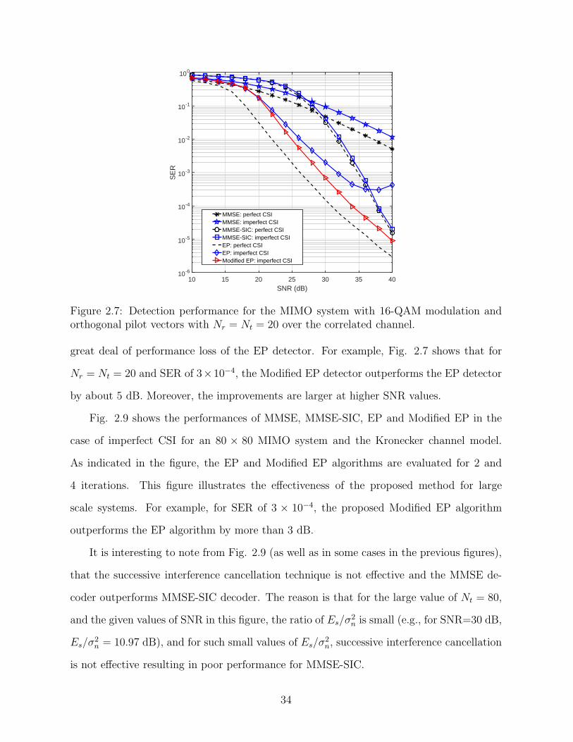
2.7 Detection performance for the MIMO system with 16-QAMmod-ulation and orthogonal pilot vectors with Nr = Nt = 20 over thecorrelated channel. . . . . . . . . . . . . . . . . . . . . . . . . . . . . . . . . . . . . . . . . . . . . . . . . . . . . . . . . . . 34
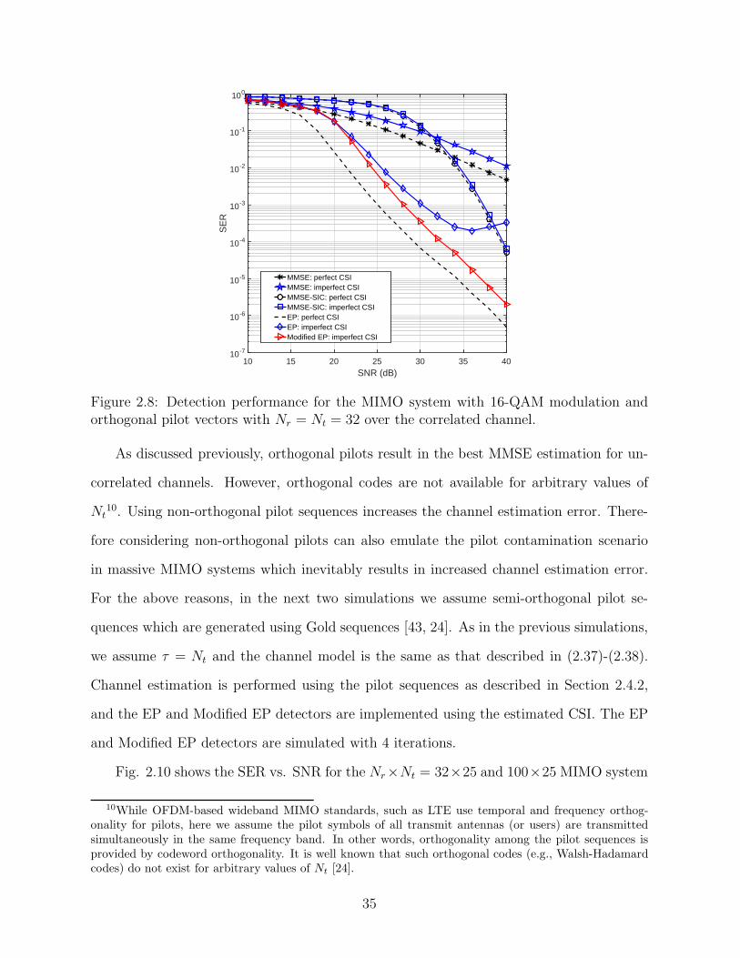
2.8 Detection performance for the MIMO system with 16-QAMmod-ulation and orthogonal pilot vectors with Nr = Nt = 32 over thecorrelated channel. . . . . . . . . . . . . . . . . . . . . . . . . . . . . . . . . . . . . . . . . . . . . . . . . . . . . . . . . . . 35
2.9 Detection performance for the MIMO system with 16-QAMmod-ulation and orthogonal pilot vectors with Nr = Nt = 80 over thecorrelated channel. . . . . . . . . . . . . . . . . . . . . . . . . . . . . . . . . . . . . . . . . . . . . . . . . . . . . . . . . . . 36
vii
2.10 Decoding performance of 32× 25 and 100× 25 MIMO systems,with imperfect CSI, 16-QAM modulations and non-orthogonalpilot vectors . . . . . . . . . . . . . . . . . . . . . . . . . . . . . . . . . . . . . . . . . . . . . . . . . . . . . . . . . . . . . . . . 37
2.11 Decoding performance of 200×30 MIMO system, with imperfectCSI, 16-QAM modulations and non-orthogonal pilot vectors . . . . . . . . . . . . . . . . . 37
3.1 Channel estimation performance of a SIMO system with Nr =100 and 8-DPSK, for pilot-based MMSE estimator, and the pro-posed EP estimator with I = 1 and block sizes T = 2, 20, 50. . . . . . . . . . . . . . . . . . 50
3.2 Detection performance of a SIMO system with Nr = 100 and 8-DPSK modulation, for coherent ML detector, coherent MMSEdetector, and noncoherent EP detector with I = 1 and blocksizes T = 2, 20, 50. . . . . . . . . . . . . . . . . . . . . . . . . . . . . . . . . . . . . . . . . . . . . . . . . . . . . . . . . . . . 51
3.3 Channel estimation performance of a SIMO system with Nr =100 and 16-DPSK modulation, for MMSE estimator with asingle-symbol pilot, and EP estimators with block sizes T = 5, 50and two different iterations I = 1 and I = 4. . . . . . . . . . . . . . . . . . . . . . . . . . . . . . . . . . 52
3.4 Detection performance of a SIMO system with Nr = 100 and 16-DPSK modulation, for MMSE estimator with a single-symbolpilot, and EP estimators with block sizes T = 5, 50 and twodifferent iterations I = 1 and I = 4. . . . . . . . . . . . . . . . . . . . . . . . . . . . . . . . . . . . . . . . . . . 53
3.5 Detection performance of coherent MMSE and noncoherent EPdetectors over Ricain fading channel with K = 10, 8-DPSKmodulation, I = 1, T = 5, and three different antenna configurations. . . . . . . . . . 53
4.1 Multi-cell multi-user MIMO network. . . . . . . . . . . . . . . . . . . . . . . . . . . . . . . . . . . . . . . . . 58
4.2 Channel estimation performance versus the receiver’s antenna-array size M , for EVD and EP estimators, with symbol blocksizes N = 20, 50, 100 and EP block size T = N . . . . . . . . . . . . . . . . . . . . . . . . . . . . . . . 75
4.3 SER performance versus the receiver’s antenna-array sizeM , forEVD and EP algorithms with symbol block sizes N = 20, 50, 100and EP block size T = N . . . . . . . . . . . . . . . . . . . . . . . . . . . . . . . . . . . . . . . . . . . . . . . . . . . . 76
4.4 Percentage of erroneous detected frames versus symbol blocksize N for a MIMO system with the receiver’s antenna-arraysize M = 100 and EP block size T = N , for EVD and EP algorithms.. . . . . . . . . 78
viii
4.5 Channel estimation performance of EVD and EP algorithms ver-sus symbol block size N for a MIMO system with the receiver’santenna-array sizes M =60,100, and EP block size T = N . . . . . . . . . . . . . . . . . . . . 79
4.6 SER performance of EVD and EP algorithms versus symbolblock size N for a MIMO system with the receiver’s antenna-array sizes M =60,100, and EP block size T = N . . . . . . . . . . . . . . . . . . . . . . . . . . . . 79
4.7 Multi-cell versus single-cell performances for EVD and EP detectors. . . . . . . . . . 80
A.1 A sample factor graph representing f1(x1)f2(x1, x4)f3(x2, x3, x4). . . . . . . . . . . . . . . 89
A.2 A sample pairwise MRF. . . . . . . . . . . . . . . . . . . . . . . . . . . . . . . . . . . . . . . . . . . . . . . . . . . . . 90
A.3 Graphical model for MIMO detection. (a) Factor Graph, (b) Messages. . . . . . . . 93
ix
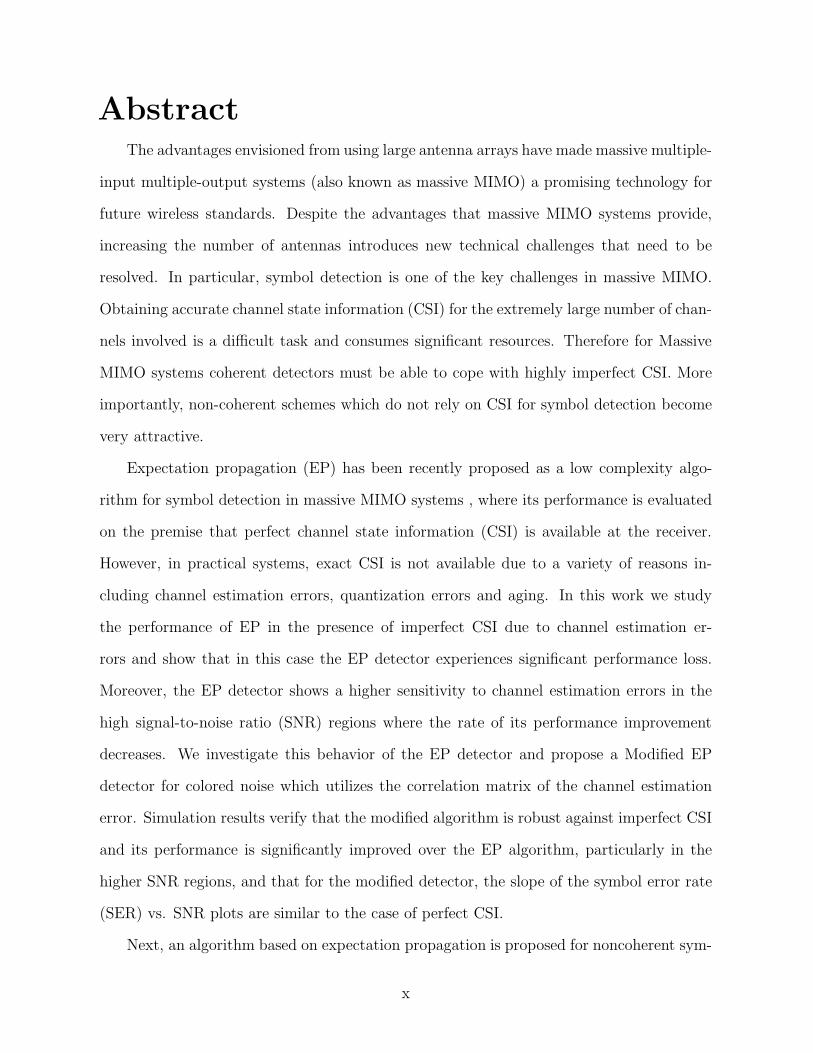
AbstractThe advantages envisioned from using large antenna arrays have made massive multiple-
input multiple-output systems (also known as massive MIMO) a promising technology for
future wireless standards. Despite the advantages that massive MIMO systems provide,
increasing the number of antennas introduces new technical challenges that need to be
resolved. In particular, symbol detection is one of the key challenges in massive MIMO.
Obtaining accurate channel state information (CSI) for the extremely large number of chan-
nels involved is a difficult task and consumes significant resources. Therefore for Massive
MIMO systems coherent detectors must be able to cope with highly imperfect CSI. More
importantly, non-coherent schemes which do not rely on CSI for symbol detection become
very attractive.
Expectation propagation (EP) has been recently proposed as a low complexity algo-
rithm for symbol detection in massive MIMO systems , where its performance is evaluated
on the premise that perfect channel state information (CSI) is available at the receiver.
However, in practical systems, exact CSI is not available due to a variety of reasons in-
cluding channel estimation errors, quantization errors and aging. In this work we study
the performance of EP in the presence of imperfect CSI due to channel estimation er-
rors and show that in this case the EP detector experiences significant performance loss.
Moreover, the EP detector shows a higher sensitivity to channel estimation errors in the
high signal-to-noise ratio (SNR) regions where the rate of its performance improvement
decreases. We investigate this behavior of the EP detector and propose a Modified EP
detector for colored noise which utilizes the correlation matrix of the channel estimation
error. Simulation results verify that the modified algorithm is robust against imperfect CSI
and its performance is significantly improved over the EP algorithm, particularly in the
higher SNR regions, and that for the modified detector, the slope of the symbol error rate
(SER) vs. SNR plots are similar to the case of perfect CSI.
Next, an algorithm based on expectation propagation is proposed for noncoherent sym-
x
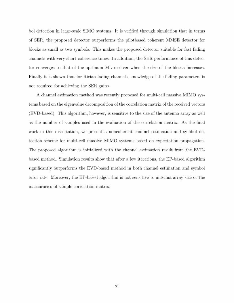
bol detection in large-scale SIMO systems. It is verified through simulation that in terms
of SER, the proposed detector outperforms the pilotbased coherent MMSE detector for
blocks as small as two symbols. This makes the proposed detector suitable for fast fading
channels with very short coherence times. In addition, the SER performance of this detec-
tor converges to that of the optimum ML receiver when the size of the blocks increases.
Finally it is shown that for Rician fading channels, knowledge of the fading parameters is
not required for achieving the SER gains.
A channel estimation method was recently proposed for multi-cell massive MIMO sys-
tems based on the eigenvalue decomposition of the correlation matrix of the received vectors
(EVD-based). This algorithm, however, is sensitive to the size of the antenna array as well
as the number of samples used in the evaluation of the correlation matrix. As the final
work in this dissertation, we present a noncoherent channel estimation and symbol de-
tection scheme for multi-cell massive MIMO systems based on expectation propagation.
The proposed algorithm is initialized with the channel estimation result from the EVD-
based method. Simulation results show that after a few iterations, the EP-based algorithm
significantly outperforms the EVD-based method in both channel estimation and symbol
error rate. Moreover, the EP-based algorithm is not sensitive to antenna array size or the
inaccuracies of sample correlation matrix.
xi
Chapter 1
Introduction
The limited resources of wireless communication systems, including the limited energy
and radio spectrum, is a major bottleneck for serving ever increasing number of users[2, 3]
and introducing new wireless services. The capabilities of multiple-antenna systems in
improving the system capacity (or throughput), bandwidth efficiency, power efficiency and
link reliability of wireless systems was first demonstrated in the vertical Bell laboratories
layered space-time (V-BLAST) project [4], as well as in early theoretical studies in [5]
and [6]. Since then and in the past two decades, multiple-antenna systems, also known
as multiple-input multiple-output (MIMO)1, have been the subject of intense academic
research and have now become an integral part of many standards. Many of the recent
wireless standards such as WiFi, WiMAX, HSPA, LTE, etc., rely on MIMO systems.
In general, improvements from MIMO systems are achieved by either combating or
exploiting the multipath fading effects of the wireless channels[7]. In spatial diversity
techniques, MIMO is used to alleviate the harmful effects of multipath scattering and to
increase communication reliability. On the other hand in spatial multiplexing, MIMO
is deployed for exploiting the signal scattering of the multipath fading channel to serve a
higher number of data streams. All MIMO-based wireless standards use one or both spatial
diversity and spatial multiplexing techniques.
The promising advantages of MIMO techniques cannot be realized without the avail-
ability of the instantaneous channel coefficients (also known as channel state information
(CSI)) either at the receiver or the transmitter. In this regard, MIMO systems can be
classified into open-loop or closed-loop systems. In an open-loop MIMO system only the
receiver needs the CSI, whereas in a closed-loop system both the receiver and the transmit-
ter use the CSI. In general, in spatial diversity MIMO receivers use CSI for data detection
1Following the similar nomenclature of MIMO, the traditional single-antenna systems are also calledsingle-input single-output (SISO).
1
and in multiplexing techniques MIMO transmitters use CSI for transmit diversity and
beamforming. Thus, depending on the availability of CSI at the receiver and/or trans-
mitter, combination of spatial techniques can be used. Table 1.1 shows examples of this
combination[7].
Table 1.1: Examples of open-loop and closed-loop MIMO systems.
Open-loop Closed-loop
Spatial Diversity Space-Time Coding (STC) Transmit Selection Diversity (TSD)
Spatial Multiplexing BLAST Eigenbeamforming
Conventional MIMO systems, which consist of one multiple-antenna transmitting node
and one multiple-antenna receiving node, are referred to as single-user MIMO (SU-MIMO)
or point-to-point MIMO. Cellular communication systrems, however, employ multi-user
MIMO (MU-MIMO), where one multiple-antenna base station (BS) serves several single-
antenna users or mobile stations (MS). Since the users in MU-MIMO are single-antenna
systems, their throughput improvement will be limited. However, the entire network will
experience increase in the overall throughput2.
1.1 Massive MIMO
Since the gains offered by MIMO systems scale with the number of transmit and receive
antennas, research on high-order MIMO (also referred to as massive MIMO) system has
been accelerated in recent years [8, 9, 10, 11]. Early studies have demonstrated the benefits
of massive MIMO systems [12], and some field trials have been carried out to show the
possibilities and limitations of this technology [13, 14, 15]. Massive MIMO is a MU-MIMO
in which the BS is equipped with an order of magnitude larger number of antennas with
respect to traditional MIMO systems. For example, while an LTE-A base station can
deploy up to 8 antennas, a massive MIMO base station may use tens or even hundreds of
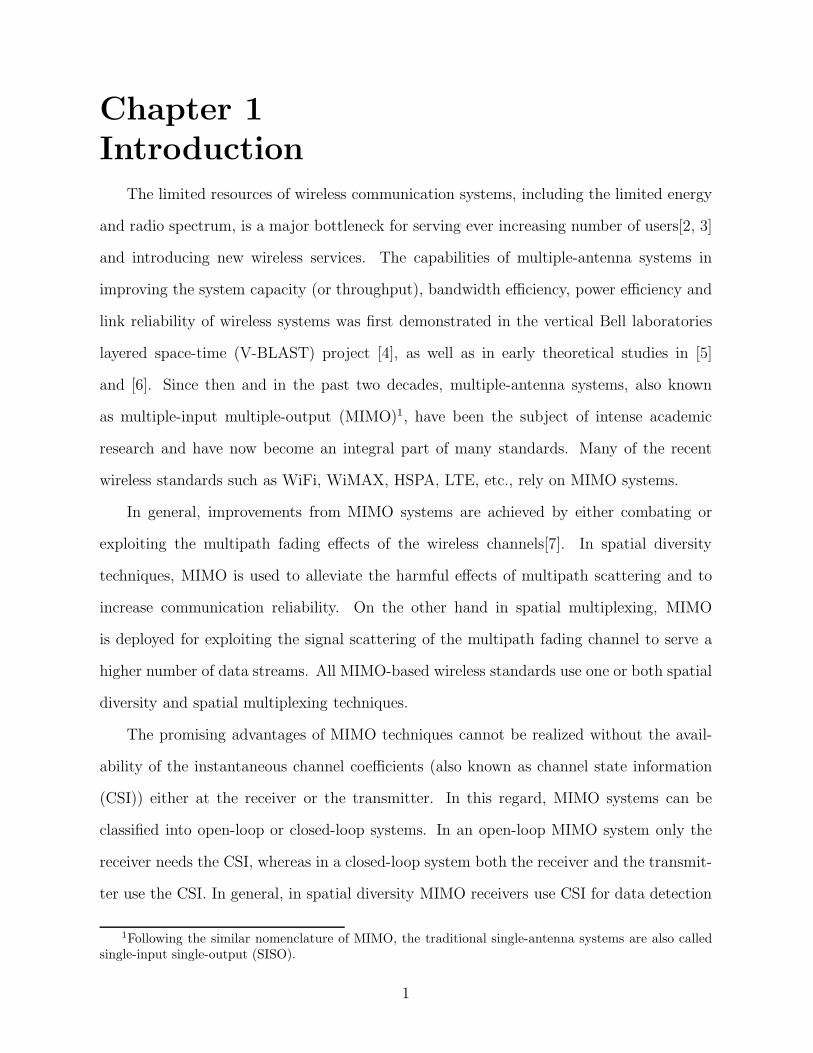
antennas. Fig. 1.1 shows a sample prototype of a massive MIMO BS at 3.7 GHz with 160
2In fact, all single-antenna nodes can be considered as an integrated node with distributed antennas.Therefore, a MU-MIMO network with single-antenna users may be viewed as a SU-MIMO system.
2
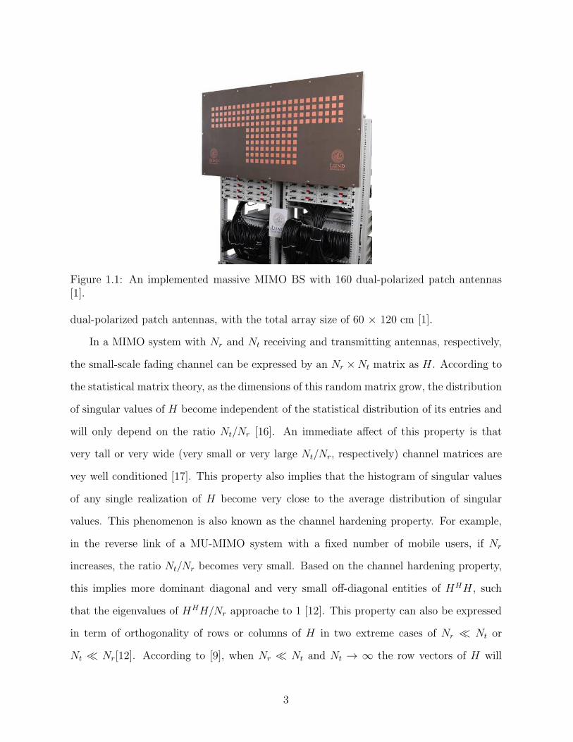
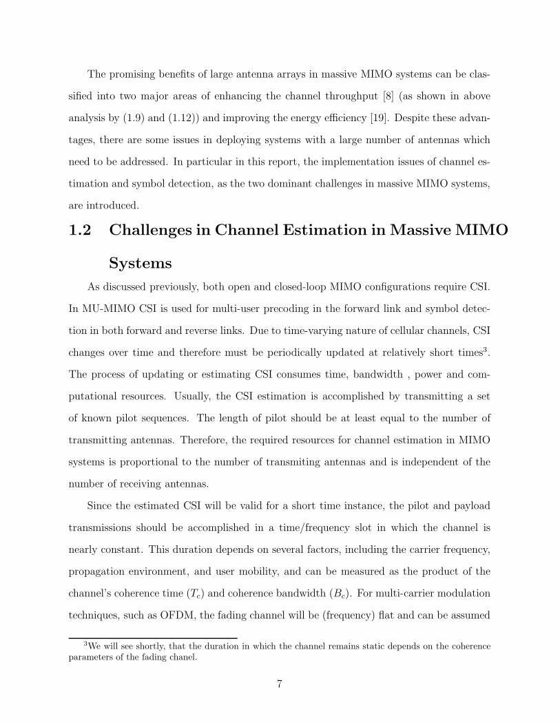
Figure 1.1: An implemented massive MIMO BS with 160 dual-polarized patch antennas[1].
dual-polarized patch antennas, with the total array size of 60 × 120 cm [1].
In a MIMO system with Nr and Nt receiving and transmitting antennas, respectively,
the small-scale fading channel can be expressed by an Nr ×Nt matrix as H . According to
the statistical matrix theory, as the dimensions of this random matrix grow, the distribution
of singular values of H become independent of the statistical distribution of its entries and
will only depend on the ratio Nt/Nr [16]. An immediate affect of this property is that
very tall or very wide (very small or very large Nt/Nr, respectively) channel matrices are
vey well conditioned [17]. This property also implies that the histogram of singular values
of any single realization of H become very close to the average distribution of singular
values. This phenomenon is also known as the channel hardening property. For example,
in the reverse link of a MU-MIMO system with a fixed number of mobile users, if Nr
increases, the ratio Nt/Nr becomes very small. Based on the channel hardening property,
this implies more dominant diagonal and very small off-diagonal entities of HHH , such
that the eigenvalues of HHH/Nr approache to 1 [12]. This property can also be expressed
in term of orthogonality of rows or columns of H in two extreme cases of Nr ≪ Nt or
Nt ≪ Nr[12]. According to [9], when Nr ≪ Nt and Nt → ∞ the row vectors of H will
3
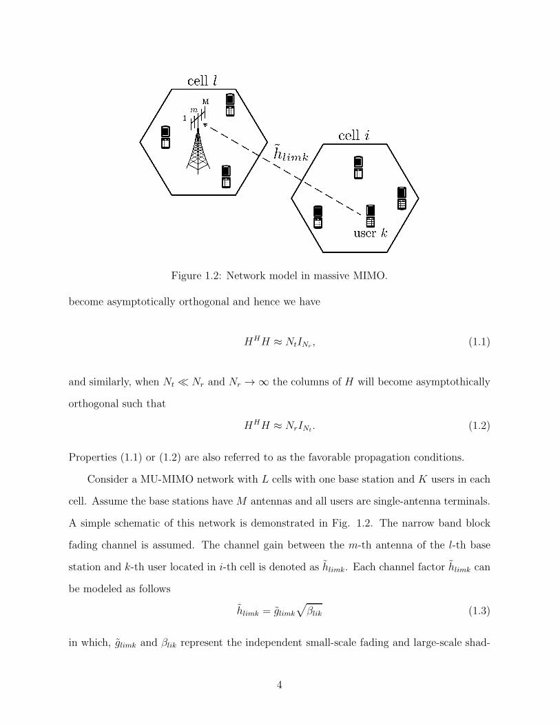
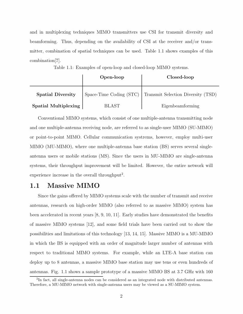
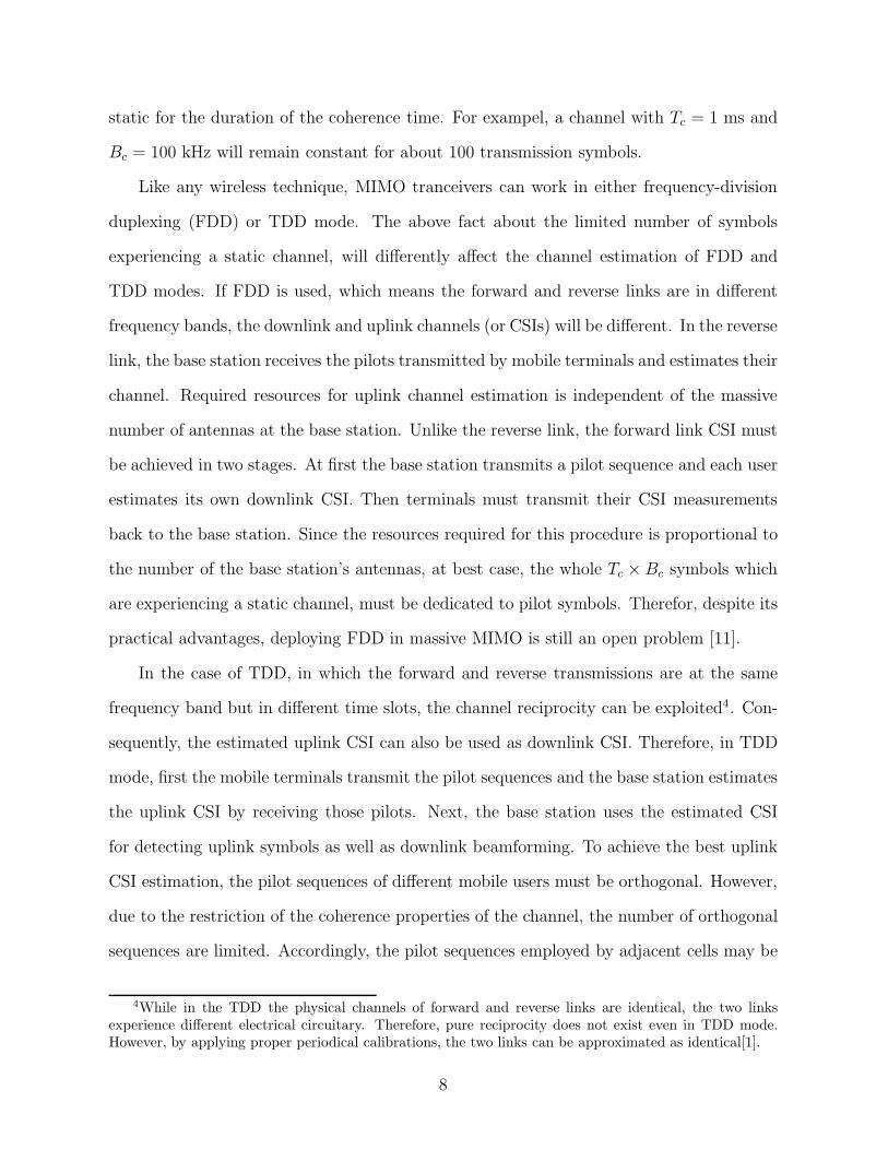
Figure 1.2: Network model in massive MIMO.
become asymptotically orthogonal and hence we have
HHH ≈ NtINr, (1.1)
and similarly, when Nt ≪ Nr and Nr → ∞ the columns of H will become asymptothically
orthogonal such that
HHH ≈ NrINt. (1.2)
Properties (1.1) or (1.2) are also referred to as the favorable propagation conditions.
Consider a MU-MIMO network with L cells with one base station and K users in each
cell. Assume the base stations have M antennas and all users are single-antenna terminals.
A simple schematic of this network is demonstrated in Fig. 1.2. The narrow band block
fading channel is assumed. The channel gain between the m-th antenna of the l-th base
station and k-th user located in i-th cell is denoted as hlimk. Each channel factor hlimk can
be modeled as follows
hlimk = glimk
√
βlik (1.3)
in which, glimk and βlik represent the independent small-scale fading and large-scale shad-
4

owing effects, respectively. In this model, glimk is the fast changing fading channel between
m-th antenna of the base station l and the k-th user in cell i, and βlik is the slow changing
shadowing gain between the l-th base station and the k-th user in cell i. As the indexes
show, βlik is independent of the base station’s array number m and is identical for all
antenna elements at the base station. Denoting glik as an M × 1 vector of small-scale
fading gains between the l-th base station and k-th user in cell i, the total fading channel
between all users of cell i and the l-th base station can be represented by theM×K matrix
Gli = [gli1 . . . gliK ]. Consequently, by including the shadowing factors, the total channel
gain is given as
Hli = GliD1
2
li (1.4)
where, Dli is a diagonal matrix with βlik values for k = 1, . . . , K on its main diagonal, i.e.
Dli =
βli1 0 . . . 0
0 βli2 . . . 0
...
0 0 . . . βliK
(1.5)
To show the effects of deploying a large number of antennas at the base stations, consider
the single-cell network, i.e. L = 1. To simplify the notations, we ignore the cell indexes.
The received vector at the base station in the reverse link is given by the following equation
y =√ρHx+ n (1.6)
in which, x is the transmitted vector of unit-energy symbols, n is the additive zero-mean
Gaussian noise with identity covariance matrix, and ρ is the signal power-to-noise power
ratio. For large M and based on the favorable channel condition in (1.2), we have
HHH ≈MD (1.7)
5
The capacity for this link is then given as
C = log2 det(IK + ρHHH), (1.8)
which by using the channel hardening property in (1.7) at large M can be simplified as [8]
C ≈K∑
k=1
log2(1 +Mρβk) bits/s/Hz. (1.9)
This formula clearly shows the dependency of the achievable throughput to M . It can
be shown that the throughput in (1.9) can be achieved by a simple matched filter (MF)
receiver [10].
By assuming time-division duplexing (TDD) mode, the transmissions over forward and
reverse links will be done in the same frequency band. Therefore, based on the channel
reciprocity property, the forward link’s channel matrix will be the transposed version of
the reverse link’s channel matrix. Consequently, the received vector for the forward link is
given as
y =√ρHTx+ n (1.10)
The capacity of this link is given by
C = maxP
log2 det(IM + ρHPHH), (1.11)
in which, P is a positive diagonal matrix of allocated powers to transmitting antennas such
as p1, . . . , pK , where∑K
k=1 pk = 1 [18]. Under the favorable channel condition and by using
the identity det(I + AAH) = det(I + AHA), the given capacity simplifies to
C ≈ maxP
log2 det(IK + ρMPD) bits/s/Hz. (1.12)
This equation demonstrates the direct dependency of the throughput to M.
6
The promising benefits of large antenna arrays in massive MIMO systems can be clas-
sified into two major areas of enhancing the channel throughput [8] (as shown in above
analysis by (1.9) and (1.12)) and improving the energy efficiency [19]. Despite these advan-
tages, there are some issues in deploying systems with a large number of antennas which
need to be addressed. In particular in this report, the implementation issues of channel es-
timation and symbol detection, as the two dominant challenges in massive MIMO systems,
are introduced.
1.2 Challenges in Channel Estimation in Massive MIMO
Systems
As discussed previously, both open and closed-loop MIMO configurations require CSI.
In MU-MIMO CSI is used for multi-user precoding in the forward link and symbol detec-
tion in both forward and reverse links. Due to time-varying nature of cellular channels, CSI
changes over time and therefore must be periodically updated at relatively short times3.
The process of updating or estimating CSI consumes time, bandwidth , power and com-
putational resources. Usually, the CSI estimation is accomplished by transmitting a set
of known pilot sequences. The length of pilot should be at least equal to the number of
transmitting antennas. Therefore, the required resources for channel estimation in MIMO
systems is proportional to the number of transmiting antennas and is independent of the
number of receiving antennas.
Since the estimated CSI will be valid for a short time instance, the pilot and payload
transmissions should be accomplished in a time/frequency slot in which the channel is
nearly constant. This duration depends on several factors, including the carrier frequency,
propagation environment, and user mobility, and can be measured as the product of the
channel’s coherence time (Tc) and coherence bandwidth (Bc). For multi-carrier modulation
techniques, such as OFDM, the fading channel will be (frequency) flat and can be assumed
3We will see shortly, that the duration in which the channel remains static depends on the coherenceparameters of the fading chanel.
7
static for the duration of the coherence time. For exampel, a channel with Tc = 1 ms and
Bc = 100 kHz will remain constant for about 100 transmission symbols.
Like any wireless technique, MIMO tranceivers can work in either frequency-division
duplexing (FDD) or TDD mode. The above fact about the limited number of symbols
experiencing a static channel, will differently affect the channel estimation of FDD and
TDD modes. If FDD is used, which means the forward and reverse links are in different
frequency bands, the downlink and uplink channels (or CSIs) will be different. In the reverse
link, the base station receives the pilots transmitted by mobile terminals and estimates their
channel. Required resources for uplink channel estimation is independent of the massive
number of antennas at the base station. Unlike the reverse link, the forward link CSI must
be achieved in two stages. At first the base station transmits a pilot sequence and each user
estimates its own downlink CSI. Then terminals must transmit their CSI measurements
back to the base station. Since the resources required for this procedure is proportional to
the number of the base station’s antennas, at best case, the whole Tc × Bc symbols which
are experiencing a static channel, must be dedicated to pilot symbols. Therefor, despite its
practical advantages, deploying FDD in massive MIMO is still an open problem [11].
In the case of TDD, in which the forward and reverse transmissions are at the same
frequency band but in different time slots, the channel reciprocity can be exploited4. Con-
sequently, the estimated uplink CSI can also be used as downlink CSI. Therefore, in TDD
mode, first the mobile terminals transmit the pilot sequences and the base station estimates
the uplink CSI by receiving those pilots. Next, the base station uses the estimated CSI
for detecting uplink symbols as well as downlink beamforming. To achieve the best uplink
CSI estimation, the pilot sequences of different mobile users must be orthogonal. However,
due to the restriction of the coherence properties of the channel, the number of orthogonal
sequences are limited. Accordingly, the pilot sequences employed by adjacent cells may be
4While in the TDD the physical channels of forward and reverse links are identical, the two linksexperience different electrical circuitary. Therefore, pure reciprocity does not exist even in TDD mode.However, by applying proper periodical calibrations, the two links can be approximated as identical[1].
8
nonorthogonal, leading to the so called pilot contamination problem[8]. We will see shortly
that unlike the intera-cell multi-user interference, which can be mitigated be employing
large antenna arrays, the inter-cell interference caused by pilot contamination cannot be
removed by increasing the number of antennas in base stations.
To show the harmful effects of pilot contamination, we can use the introduced multi-cell
massive MIMO model in Fig. 1.2. Assume the worst case scenarion, in which mobile users
synchronously and simultaneously transmit pilot sequences for uplink channel estimation.
As another important assumption, suppose the complete intera-cell orthogonality among
pilots and that the identical set of pilots are used in all cells. By assuming τ as the length
of pilots, the pilot sequence of the k-th users in all cell can be considered by a 1 × τ row
vector denoted as pk. Consequently, we can represent the matrix of all K orthogonal pilots
inside each cell by P = [pT1 , . . . ,p
TK ]
T , which is a K× τ matrix. By intra-cell orthogonality
we have PPH = τIK . Without loss of generality, assume the uplink channel estimation in
the first base station, i.e. l = 1. From (1.6) and by the above assumptions, the received
matrix at this base station can be written as
Y1 =√ρ
L∑
l=1
H1lP +N1 (1.13)
where H1l ∈ CM×K is defined in (1.4), and N1 ∈ CM×K is the additive noise matrix of the
first base station during the pilot transmission.
For channel estimation, the target base station must project the received signals to the
space of orthogonal pilots. This can be implemented by multiplying the received matrix
by the PH [10]. Therefore, H11 as the estimation of H11 is given as
H11 =1
τ√ρY1P
H (1.14)
= H11 +∑
i 6=l
Hil +1
τ√ρN1P
H (1.15)
9
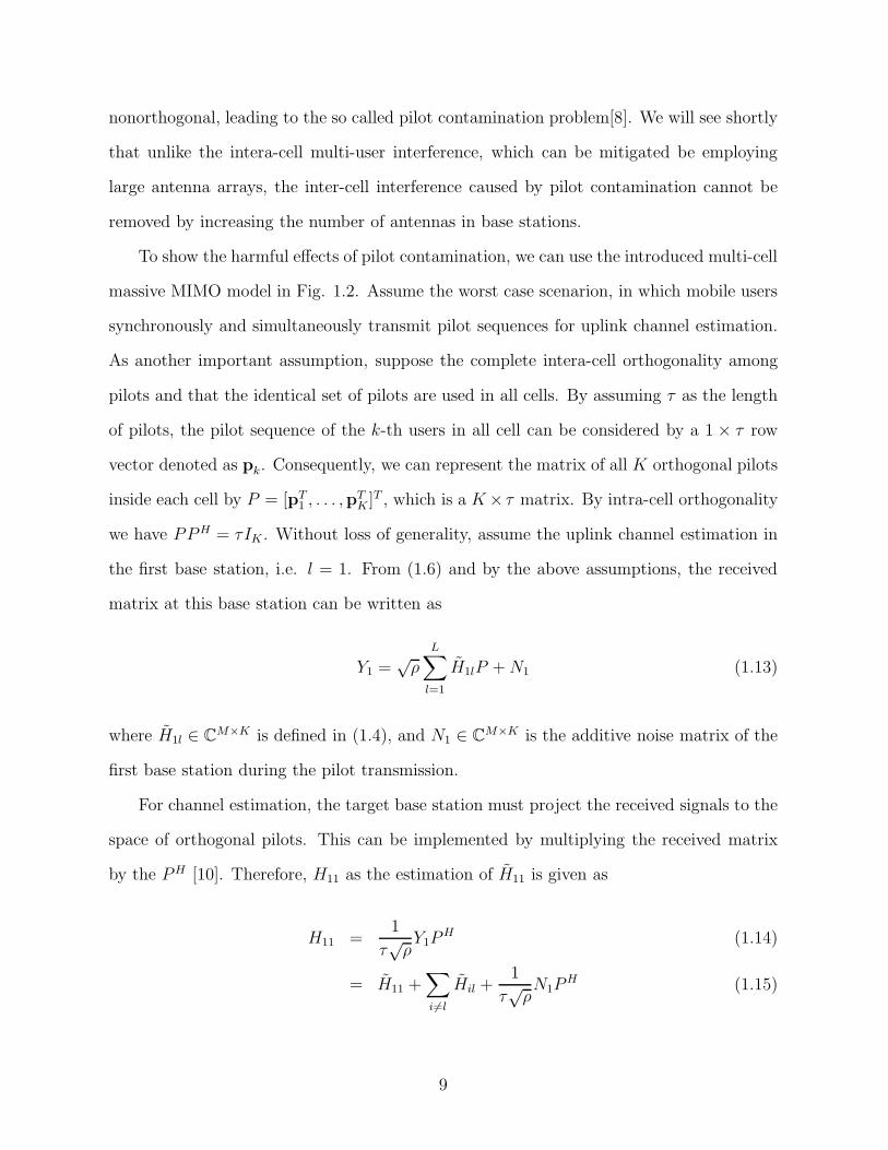
(a) (b)
Figure 1.3: Direct inter-cell reverse link interference due to pilot contamination. (a) Per-fect beamforming (without pilot contamination), (b) distorted beamforming (with pilotcontamination).
The second term in the right hand side of (1.15) shows the effect of pilot contamination
which appears as an extra noise to the final estimation. Considering that all variables in this
model are complex-valued, reveals that even a small complex noise can adversely affect the
phase of resultant estimations. Since the base station uses this estimation for beamforming
in forward link, the channel estimation error creates directional side-lobes toward the other
users in adjacent cells, which will be an important source of directional interference. While
the intra-cell interference can be mitigated by deploying massive MIMO, the harmful effects
of this inter-cell interference cannot be alleviated by increasing the number of antennas.
This issue is depicted in Fig. 1.3.
In addition to estimation errors, CSI is subject to errors due to aging and quantization
[20, 21, 22, 23]. Therefore, assuming perfect CSI in analysis may lead to incorrect or
infeasible results.
10
1.3 Challenges in Symbol Detection in Massive MIMO
Systems
Symbol estimation and detection in MIMO is generally a challenging process. To make
it more clear, lets consider the reverse link of a MU-MIMO system, as in (1.6). In this
model, the base stations receives the M × 1 vector y and should detect the transmitted
symbols in the K× 1 vector x. Assuming M-ary modulation scheme, symbols are selected
from the constellation set AM. If we assume a coherent detection mechanism in which
the perfect CSI is available at the basestation, and that transmitted symbols are equally
probable, the maximum likelihood (ML) detection rule is given as
xML = argmaxx∈AK
M
p(y|x, H) (1.16)
To solve this optimization problem, the receiver must search MK different K-tuples
with elements in AM. Therefore, the optimum MIMO detection by ML is essentially an
exhaustive search method which is an NP-hard problem and its complexity increases ex-
ponentially with the number of transmitters and the modulation order. Moreover, the
performance of linear schemes such as zero-forcing (ZF) and minimum-mean-squared-error
(MMSE) decoders (which have polynomial-time complexity [24]) is poor. Successive inter-
ference cancellation (SIC) was shown to improve the performance of ZF in the early MIMO
project V-BLAST [25] and later was extended to MMSE [26]. However, the performances
of MMSE-SIC and ZF-SIC are still far from that of the ML decoder.
Masive MIMO, on the other hand, by employing an order of magnitude more antennas
at the base station provides an opportunity for deploying linear detectors. As is shown in
[8], under the favorable channel condition, the capacity in (1.9) is achievable by using a
simple linear matched filter detector. This fact can also be understood intuitively. Since
in favorable channel conditions the channel vectors of different users become mutually
orthogonal, the receiver will be able to remove the interference with deploying even a
11
simple linear algorithm. As explained before, favorable propagation condition will occur
in presense of two extreme cases of very large antenna array (Nr → ∞) and very small
number of transmitters (Nt ≪ Nr). However, in many real propagation environments,
increasing Nr does not necessarily creates orthogonality [27]. Moreover, to increase the
system’s spectral efficiency, it is more appealing to serve larger number of users. These
facts reveal the possible practical restrictions in using linear detectors in massive MIMO
systems. Therefore, nonlinear detection algorithms which provide better performance at
the cost of higher complexity, are still possible solutions for symbol detection in massive
MIMO systems [10].
1.4 Outline of the Dissertation
The rest of this dissertation is organized as follows. In Chapter 2, we introduce the
recently suggested MIMO detection technique based on Expectation Propagation. We will
show that the proposed algorithm is very sensitive to the quality of the channel state infor-
mation at the receiver. Therefore, a modification to the algorithm is suggested to enhance
the detector’s robustness against the incomplete knowledge of the channel coefficients at
the receiver.
A noncoherent detector, based on the Expectation Propagation algorithm, is suggested
for Single Input Multiple Output (SIMO) systems in Chapter 3. The inherent phase am-
biguity in the estimated channel coefficients can be bypassed by employing differentially
encoded modulation symbols. It is shown that the algorithm can easily outperform the
coherent Minimum Mean Square Error (MMSE) detectors. Also, the performance of the
optimum Maximum Likelihood (ML) detector is achievable with large enough blocks.
In Chapter 4 a joint channel estimation and symbol detection algorithm based on the
Expectation Propagation is suggested for multi-user multi-cell MIMO systems. It is shown
that by initializing the Expectation Propagation algorithm with results of a rough and
inaccurate noncoherent channel estimator, such as the EVD-based algorithm, considerable
improvements in channel estimation and symbol detection performances is achieved. It is
12

also shown that the combination of the two algorithms can significantly decrease the overall
rate of erroneous blocks. Finally, the conclusions are given in Chapter 5.
13
Chapter 2
MIMO DetectionWith Imperfect
Channel State Information Using
Expectation Propagation
2.1 Introduction
Multiple-input multiple-output (MIMO) technology can significantly increase system
capacity (throughput) and improve the reliability of wireless communication systems, and
is now incorporated into many wireless standards such as WiFi, WiMAX, LTE, etc. Since
the gains offered by MIMO systems scale with the number of transmit and receive antennas,
research on high-order MIMO (also referred to as massive MIMO) has been accelerated in
recent years [8, 9, 10]. Early studies have demonstrated the benefits of massive MIMO
systems [12], and some field trials have been carried out to show the possibilities and
limitations of this technology [13, 14, 15].
In massive MIMO systems employing a high-order modulation scheme, symbol detec-
tion is a particularly challenging problem. The complexity of the optimal maximum likeli-
hood (ML) decoder is exponential in the number of transmit antennas and it is essentially an
exhaustive search method. Moreover, the performance of linear schemes such as zero-forcing
(ZF) and minimum-mean-squared-error (MMSE) decoders (which have polynomial-time
complexity [24]) is poor. Successive interference cancellation (SIC) was shown to improve
the performance of ZF in the early MIMO project V-BLAST [25] and later was extended
to MMSE [26]. However, the performances of MMSE-SIC and ZF-SIC are still far from
that of the ML decoder.
It is shown in [12] that for a fixed number of transmit antennas Nt1, as the number of
receive antennas Nr increases, the channel vectors become orthogonal. This phenomenon
referred to as channel hardening occurs when the loading factor Nt
Nr<< 1. Therefore for
1Equivalently, a fixed number of synchronous single-antenna users.
14
such systems simple linear detectors such as ZF and MMSE detectors show acceptable
performance [8]. However, the spectral efficiency of these systems is low due to the small
number of transmit antennas Nt. On the other hand, increasing Nt improves the system
spectral efficiency, but severely degrades the performance of linear decoders.
Graph-based statistical inference techniques such as Belief Propagation (BP) have
proven to be powerful tools for detection problems and also practically viable, particularly
in models with a large number of variables or high degrees of freedom [28]. Unfortunately,
when the underlying graph has many short cycles, the performance of these algorithms is
not satisfactory; and the graph corresponding to symbol detection in MIMO systems is a
fully connected graph [29]. To overcome this difficulty, in [29] the authors find a Gaussian
Tree Approximation (GTA) on the posterior distribution of the transmitted symbols. The
BP algorithm is then used to compute an approximation of this posterior distribution. In
[30] GTA has been enhanced with successive interference cancellation (GTA-SIC).
More recently the Expectation Propagation (EP) algorithm of [31] has been applied
to symbol detection in MIMO systems [32]. Briefly, EP attempts to find the closest ap-
proximation for the conditional marginal distribution of a desired variable in an iterative
refinement procedure. Therefore, it can be employed in MIMO detection for finding the
posterior distribution of the transmitted symbols. As shown in [32], in terms of symbol error
probability, the EP detector outperforms other detectors such as GTA-SIC and MMSE-SIC
with low complexity2.
The performance of EP in [32] is evaluated on the premise that perfect channel state
information (CSI) is available at the receiver. However, in MIMO systems, channel coeffi-
cients are typically estimated at the receiver from finite-length pilot sequences [33, 34]. In
cellular networks using massive MIMO systems, pilot interference from neighboring cells
limits the accuracy of channel estimation giving rise to the so-called pilot contamination
problem [35]. In addition to estimation errors, CSI is subject to errors due to aging and
2For a careful comparison of the computational complexity of the above algorithms we refer the readerto [32].
15
quantization [20, 36, 22, 23]. In [37] the authors formulate the ML decoder under imperfect
CSI and propose recursive tree search algorithms for the implementation of their decoders.
Degradation of the performance of ZF in the case of imperfect CSI is analyzed in [23].
However, to the best of our knowledge, the performance of EP algorithm under imperfect
CSI has not been studied.
In this paper we show that although channel estimation improves by increasing the
signal-to-noise ratio (SNR), surprisingly, at high SNR values, the rate of improvement
of symbol error rate (SER) vs. SNR decreases. We investigate this behavior of the EP
detector in the case of imperfect CSI and propose a modified detector in order to recover
some of the performance loss of the EP detector. Simulation results verify that the proposed
modification improves the performance of EP in the case of imperfect CSI, particularly in
higher SNR regions, and that for the modified detector the slope of the SER vs. SNR plots
are similar to the case of perfect CSI.
The rest of this chapter is organized as follows. The system model is presented in
Section 2.2. A brief review on the EP algorithm is presented in Section 2.3. Section
2.4 contains the derivation of EP for the general model with imperfect CSI followed by
the calculations of covariance matrix of channel estimation error. Finally the simulation
results are presented in Sections 2.5.
Notations: Throughout this paper, small letters (x) are used for scalars, bold small
letters (x) for vectors, and capital letters (X) denote matrices. R and C represent the set
of real and complex numbers, respectively. R(z) and I(z) denote the real and imaginary
parts of the complex variable z. For a set of complex variables A = {z1, z2, · · · }, we denote
R(A) , {R(z1),R(z2), · · · } and I(A) , {I(z1), I(z2), · · · }. The superscripts (.)T , (.)H ,
and (.)−1 represent transpose, Hermitian transpose, and matrix inverse, respectively. Also,
⊗ denotes the matrix Kronecker product. For a probability density function (PDF) p(.),
Ep denotes the expectation operator with respect to p(.). IN denotes the N × N identity
matrix. Finally, vec(A) and ||a|| denote the vectorization of the matrix A and the ℓ2 norm
16
of vector a, respectively.
2.2 System Model
Consider a MIMO system with Nr and Nt receive and transmit antennas, respectively3.
The vector of transmitted symbols at each channel use is denoted as u = [u1, . . . , uNt]T ∈
CNt×1, where ui’s are symbols from an M-ary modulation constellation AM with av-
erage energy Es. The channel matrix denoted by H ′ ∈ CNr×Nt is a realization from
a zero-mean complex symmetric Gaussian distribution with covariance matrix Rh, i.e.,
h′= vec(H ′) ∼ CN (h
′|0, Rh). We assume a block fading channel where the channel ma-
trix H ′ remains constant for the duration of a transmission block which includes several
transmission vectors.
The received vector y is given by
y = H ′u+ n, (2.1)
where y ∈ CNr×1, and n ∈ CNr×1 is the zero-mean white Gaussian noise vector with
n ∼ CN (n|0, σ2nINr
). Assuming independent and identically distributed (iid) transmitted
symbols, the a posteriori distribution of the transmitted symbols is given by
p(
u|y, H ′)
∝ N(
y|H ′u, σ2nINr
)
Nt∏
i=1
Iui∈AM(2.2)
in which IA is the indicator function of the event A.
We denote the receiver’s estimate of the channel matrix by H . Therefore, the receiver’s
view of the model in (2.1) is given by
y = Hu+ n. (2.3)
Consequently, the receiver assumes that the a posteriori distribution of the transmitted
3This model is also applicable to a multi-user system in which Nt single-antenna users synchronouslytransmit to an Nr-antenna receiver.
17
symbols is given by
p(
u|y, H)
∝ N(
y|Hu, σ2nINr
)
Nt∏
i=1
Iui∈AM. (2.4)
The distributions in (2.2) and (2.4) have a multiplicative form with respect to the unknown
variables which makes it suitable for employing the EP algorithm [31]. However, it should
be noted that the receiver assumes the a posterior distribution in (2.4) an it is to this
form that the EP algorithm will be applied. In Section 2.4.1 we describe the deleterious
consequences of this approach.
2.3 Expectation Propagation
EP is an iterative algorithm for finding the best approximation to a desired distribution
from within a tractable family of distributions.
Following the proposed algorithm in [38] and [31], suppose the parameter θ must be
estimated from some independent measurements x1, . . . , xn. As is common in Bayesian
estimation, it is assumed that the prior distribution of θ is known. Therefore the posterior
distribution is given by
p(θ|x1, . . . , xn) ∝ p(θ)n∏
i=1
p(xi|θ) ,n∏
i=0
pi(θ) (2.5)
where p0(θ) , p(θ) and pi(θ) , p(xi|θ) for i = 1, 2 · · · , n. EP exploits this factorized
structure for approximating the above conditional distribution by a distribution from the
exponential family, q(θ), of the form
q(θ) ∝n∏
i=0
qi(θ) (2.6)
where qi(θ), i = 0, 1, · · · , n is from an exponential family. Several properties of the ex-
ponential family are helpful in simplifying the computations. Two of these properties are
extensively used in the computations involved in EP. First is that as in (2.6), multiplication
18
(or division) of two exponential distributions results in an exponential distribution. More-
over, the parameters of the resulting distribution are easily computed from the parameters
of the constituent distributions. Next, the EP algorithm tries to iteratively find the closest
q(θ) to the distribution p(θ|x1, . . . , xn) where closeness is in terms of the Kullback–Leibler
divergence. Therefore, q(θ) is the solution of the following optimization problem:
q∗(θ) = argminq∈F
KL(p(θ|x1, . . . , xn)‖q(θ)) (2.7)
where F is a family of exponential distributions. It turns out that when F is the exponential
family with sufficient statistics T1(θ), T2(θ), . . . , TS(θ), then the solution of (2.7) is obtained
from the moment matching condition, namely
Eq[Ti(θ)] = Ep[Ti(θ)], i = 1, 2, . . . , S (2.8)
In other words in each step of the optimization we need to match the moments between q(θ)
and p(θ|x1, · · · , xn). For example if we choose q(θ) from the family of normal distributions,
this is equivalent to equating the mean and variance of q(θ) and p(θ|x1, . . . , xn). However,
EP implements this process in a subtle way, in which instead of finding the best q(θ) at once,
it finds the best factors of q(θ) one by one and refines them through successive iterations.
At first, the algorithm starts by initializing all the factors qi(θ) and consequently q(θ) itself.
Denoting the computed q(θ at the lth iteration by q(l)(θ), then all the factors of q(l)(θ) are
updated as follows. To update the i-th factor, a so called cavity distribution4 is derived, in
which the effect of the ith factor is eliminated from q(l)(θ). Therefore, the i-th cavity PDF
is given by
q\i(θ) =q(l)(θ)
q(l)i (θ)
(2.9)
Then by combining pi(θ), the i-th factor of p(θ|x1, . . . , xn), and this cavity factor, a new
4Also known as partial belief.
19
intermediate distribution is obtained as
pi(θ) =1
Ziq\i(θ)pi(θ) (2.10)
in which Zi = Eq\i [pi(θ)] =∫ +∞
−∞pi(θ)q
\i(θ) dθ. Since in general pi(θ) and consequently pi(θ)
are not members of the exponential family, the algorithm now finds the closest distribution
from the exponential family, qnew(θ), to pi(θ) using the moment matching condition. After
calculating qnew(θ), the refined version of the i-th factor is obtained as
q(l+1)i (θ) = Zi
qnew(θ)
q\i(θ)(2.11)
After updating all the factors q(l+1)i (θ), i = 0, 1, · · · , n, q(l+1)(θ) is obtained using (2.6), and
the process is repeated with the next iteration and until a termination criterion is satisfied.
The above procedure is summarized in Algorithm 1. Finally, if we denote the output of
the EP algorithm by q(θ), the parameter θ is estimated as θ = Eq[θ].
Data: The main conditional PDF from (2.5)Result: A member of exponential family as (2.6) which is closest to (2.5)begin
Initialize all qi factors;Calculate q by (2.6);while termination criteria has not been met do
for i=0,. . . ,n do
Calculate the cavity PDF by (2.9);Calculate the new intermediate PDF by (2.10);Find qnew by moment matching;Update the i-th factor by (2.11);Update q by (2.6);
end
end
end
Algorithm 1: EP algorithm
20
2.4 EP algorithm for imperfect CSI
2.4.1 Motivation
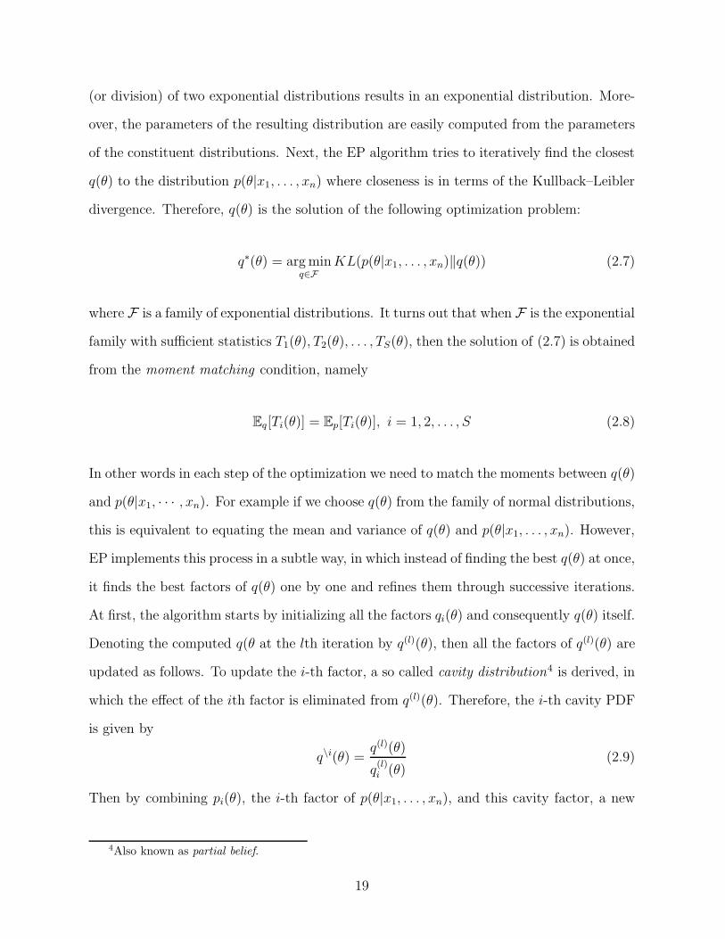
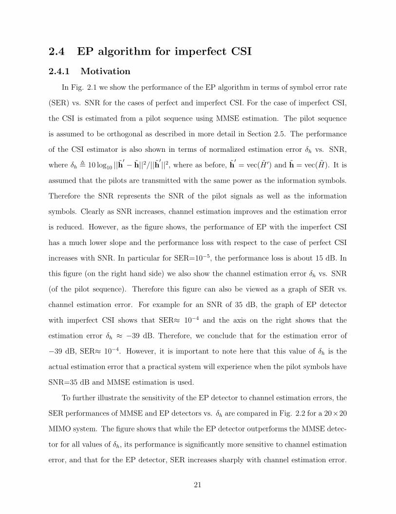
In Fig. 2.1 we show the performance of the EP algorithm in terms of symbol error rate
(SER) vs. SNR for the cases of perfect and imperfect CSI. For the case of imperfect CSI,
the CSI is estimated from a pilot sequence using MMSE estimation. The pilot sequence
is assumed to be orthogonal as described in more detail in Section 2.5. The performance
of the CSI estimator is also shown in terms of normalized estimation error δh vs. SNR,
where δh , 10 log10 ||h′ − h||2/||h′||2, where as before, h
′= vec(H ′) and h = vec(H). It is
assumed that the pilots are transmitted with the same power as the information symbols.
Therefore the SNR represents the SNR of the pilot signals as well as the information
symbols. Clearly as SNR increases, channel estimation improves and the estimation error
is reduced. However, as the figure shows, the performance of EP with the imperfect CSI
has a much lower slope and the performance loss with respect to the case of perfect CSI
increases with SNR. In particular for SER=10−5, the performance loss is about 15 dB. In
this figure (on the right hand side) we also show the channel estimation error δh vs. SNR
(of the pilot sequence). Therefore this figure can also be viewed as a graph of SER vs.
channel estimation error. For example for an SNR of 35 dB, the graph of EP detector
with imperfect CSI shows that SER≈ 10−4 and the axis on the right shows that the
estimation error δh ≈ −39 dB. Therefore, we conclude that for the estimation error of
−39 dB, SER≈ 10−4. However, it is important to note here that this value of δh is the
actual estimation error that a practical system will experience when the pilot symbols have
SNR=35 dB and MMSE estimation is used.
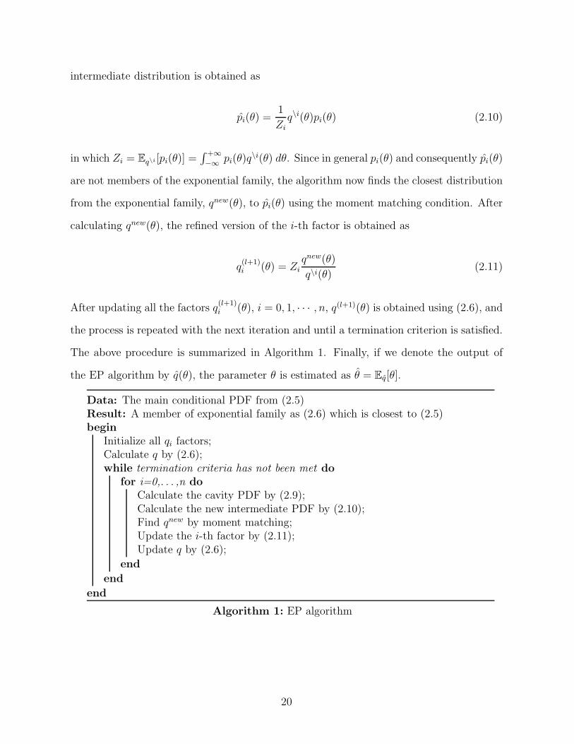
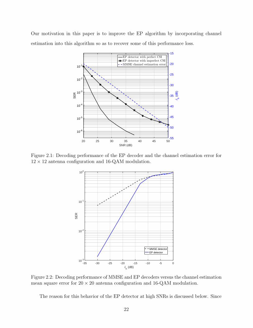
To further illustrate the sensitivity of the EP detector to channel estimation errors, the
SER performances of MMSE and EP detectors vs. δh are compared in Fig. 2.2 for a 20×20
MIMO system. The figure shows that while the EP detector outperforms the MMSE detec-
tor for all values of δh, its performance is significantly more sensitive to channel estimation
error, and that for the EP detector, SER increases sharply with channel estimation error.
21
Our motivation in this paper is to improve the EP algorithm by incorporating channel
estimation into this algorithm so as to recover some of this performance loss.
20 25 30 35 40 45 50SNR (dB)
10-6
10-5
10-4
10-3
10-2
10-1
SE
R
-55
-50
-45
-40
-35
-30
-25
-20
-15
δh (
dB)
EP detector with perfect CSI
EP detector with imperfect CSI
MMSE channel estimation error
Figure 2.1: Decoding performance of the EP decoder and the channel estimation error for12× 12 antenna configuration and 16-QAM modulation.
-35 -30 -25 -20 -15 -10 -5 0δ
h (dB)
10-3
10-2
10-1
100
SE
R
MMSE detectorEP detector
Figure 2.2: Decoding performance of MMSE and EP decoders versus the channel estimationmean square error for 20× 20 antenna configuration and 16-QAM modulation.
The reason for this behavior of the EP detector at high SNRs is discussed below. Since
22

the receiver’s view of the a posteriori distribution is given by (2.4), the EP algorithm starts
by replacing the non-Gaussian factors in (2.4) by (unnormalized) Gaussian factors to get
q(u) ∝ N(
y|Hu, σ2nINr
)
Nt∏
i=1
eγiui−Γiu2i /2 (2.12)
The constants γi and Γi > 0 are then computed iteratively from the EP algorithm [32].
However, as mentioned previously, the true a posteriori distribution is given by (2.2). In
other words, the actual mean of the received vector is located at H ′u. However, due to the
imperfect CSI, the receiver search area is centered around Hu, as shown in Fig. 2.3(a).
As SNR increases, the distance between the actual mean and the center of the search area,
given by ‖(H ′− H)u‖, increases5. Equivalently we may consider that the distance remains
the same but the search area becomes smaller6. This makes it more difficult for EP to find
a good approximation to the true a posterior distribution. As a result the performance is
degraded. Furthermore, increasing the SNR does not alleviate this problem. Obviously, as
SNR goes to infinity, the two SER curves meet. However, as our results show, this does
not occur for practical values of SNR.
In order to address this problem and to modify the EP algorithm for the case of
imperfect CSI, in the next section we discuss the problem of MIMO channel estimation
based on a pilot sequence. We will show that by taking into consideration the channel
estimation error, the search area can be aligned toward the actual mean as in Fig. 2.3(b),
which leads to a much better detection performance and lower sensitivity of the algorithm
to imperfect CSI.
2.4.2 Channel estimation
Due to its simplicity and accuracy, MMSE is commonly used in many pilot-based
channel estimation applications. Therefore, we assume that at the receiver CSI is obtained
5In practice, an increase in SNR is due to an increase in transmit power Es.6In other words, we may assume that the transmit power remains constant and the increase in SNR is
due to a reduction in noise power.
23
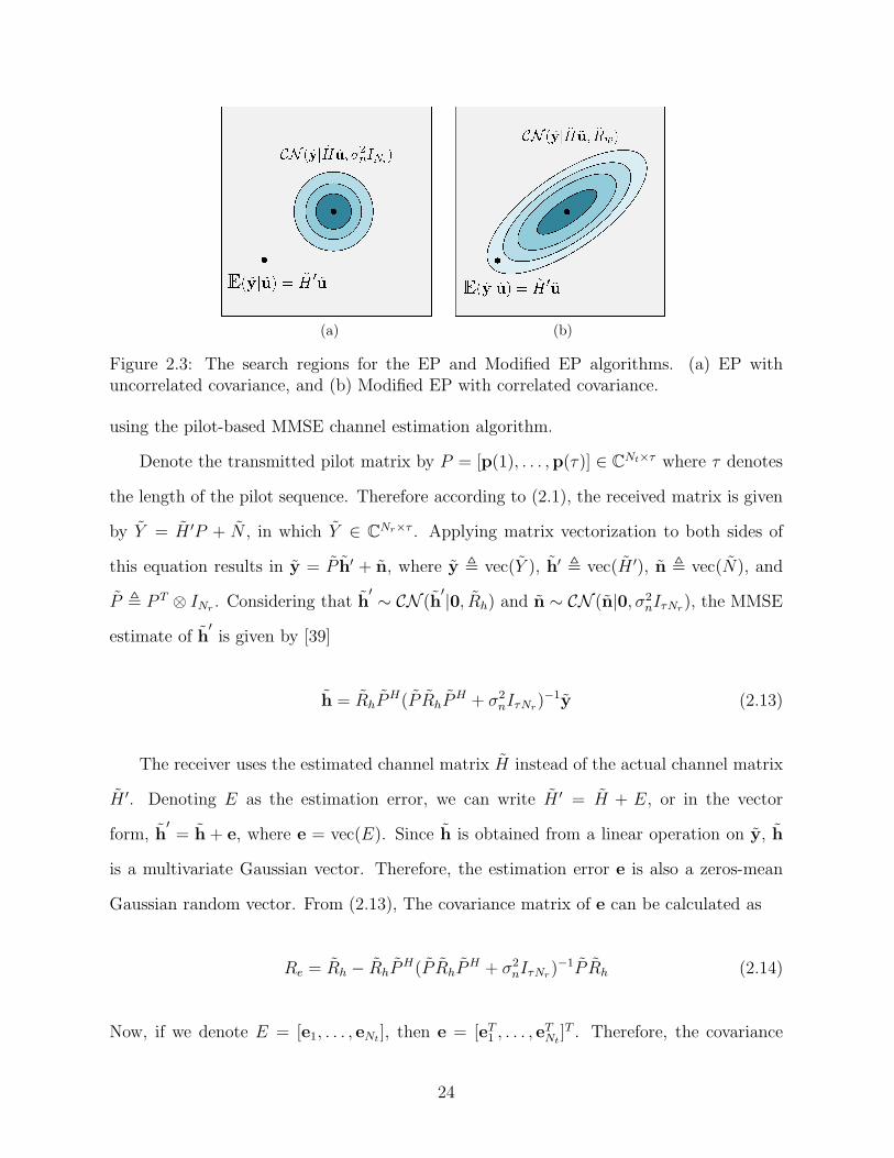
(a) (b)
Figure 2.3: The search regions for the EP and Modified EP algorithms. (a) EP withuncorrelated covariance, and (b) Modified EP with correlated covariance.
using the pilot-based MMSE channel estimation algorithm.
Denote the transmitted pilot matrix by P = [p(1), . . . ,p(τ)] ∈ CNt×τ where τ denotes
the length of the pilot sequence. Therefore according to (2.1), the received matrix is given
by Y = H ′P + N , in which Y ∈ CNr×τ . Applying matrix vectorization to both sides of
this equation results in y = P h′ + n, where y , vec(Y ), h′ , vec(H ′), n , vec(N), and
P , P T ⊗ INr. Considering that h
′ ∼ CN (h′|0, Rh) and n ∼ CN (n|0, σ2
nIτNr), the MMSE
estimate of h′is given by [39]
h = RhPH(P RhP
H + σ2nIτNr
)−1y (2.13)
The receiver uses the estimated channel matrix H instead of the actual channel matrix
H ′. Denoting E as the estimation error, we can write H ′ = H + E, or in the vector
form, h′= h + e, where e = vec(E). Since h is obtained from a linear operation on y, h
is a multivariate Gaussian vector. Therefore, the estimation error e is also a zeros-mean
Gaussian random vector. From (2.13), The covariance matrix of e can be calculated as
Re = Rh − RhPH(P RhP
H + σ2nIτNr
)−1P Rh (2.14)
Now, if we denote E = [e1, . . . , eNt], then e = [eT1 , . . . , e
TNt]T . Therefore, the covariance
24
matrix of e can be written as
Re =
R1,1 . . . R1,Nt
......
RNt,1 . . . RNt,Nt
(2.15)
in which Ri,j , E[eieHj ].
It can be verified that RE , E[EEH ] =∑Nt
i=1Ri,i. Therefore, after calculating Re from
(2.14), RE can be calculated by adding the Nt matrices of size Nr×Nr located on the main
diagonal of Re.
From the system model in (2.1), we can write
y = Hu+ w (2.16)
where w ∈ CNr×1 is a new additive noise vector defined as w = Eu + n. Assuming a
symmetric modulation set such as QAM, for which E[u] = 0, we get E[w] = 0 and
Rw = EsRE + σ2nINr
, (2.17)
Considering the fact that the off-diagonal elements of RE may be non-zero, w must be
treated as colored noise. In the case of perfect CSI, the channel estimation error is zero
and, consequently, Rw = σ2nINr
. In this case the EP algorithm has very good performance
and in fact outperforms other algorithms including GTA [32]. However, in the case of
imperfect CSI, Rw is given by (2.17) and as discussed previously, the EP algorithm has
a significant performance loss. In the next section we present a Modified EP algorithm
for colored noise which is very effective in reducing the sensitivity of the EP algorithm to
channel estimation errors.
25
To simplify notation, we transform (2.16) into an all-real equation as follows
R(y)
I(y)
=
R(H) −I(H)
I(H) R(H)
R(u)
I(u)
+
R(w)
I(w)
(2.18)
Equivalently, this can be written as y = Hu + w with y ∈ R2Nr×1, H ∈ R2Nr×2Nt ,
u ∈ R2Nt×1, and finally w ∈ R2Nr×1. In this model, the elements of u belong to AM =
R(AM) ∪ I(AM). In the case of symmetric M-ary QAM, AM can be considered as the set
of underlying PAM symbols with average energy of 0.5Es. Moreover, the covariance matrix
of w is given by
Rw =
12Rw 0
0 12Rw
(2.19)
Similar to (2.4), the a posteriori PDF for this model is given by
p(u|y, H) ∝ N (y|Hu, Rw)2Nt∏
i=1
Iui∈AM. (2.20)
In the following section the proposed algorithm in [32] is extended into this more general
model.
2.4.3 EP formulation for correlated noise channel
Following the standard methodology of EP algorithm introduced in Section 2.3, the
algorithm exploits the factorized form of (2.20) by replacing each factor by a member of the
exponential family of distributions. Next, the algorithm refines each factor by applying the
moment matching condition. Therefore, we replace each factor Iui∈AMin (2.20) by a Gaus-
sian PDF qi(ui) = N (ui|mi, ψi), in which mi and ψi ≥ 0 are the mean and variance of the
distribution, respectively. As a result, the a posteriori PDF in (2.20) can be approximated
by q(u) ∝ N (y|Hu, Rw)∏2Nt
i=1 qi(ui), which we write as
q(u) ∝ N (y|Hu, Rw) exp(uTm− 1
2uTV u), (2.21)
26
wherem = [m1/ψ1, . . . , m2Nt/ψ2Nt
]T , and V is a diagonal matrix given by V = diag(1/ψ1, . . . , 1/ψ2Nt).
Now (2.21) can be written as
q(u) ∝ N (u|µ,Σ) (2.22)
with the covariance matrix Σ and the mean vector µ where
Σ = (HTR−1w H + V )−1 (2.23)
and,
µ = Σ(HTR−1w y+m) (2.24)
Since the factors qi(ui), i = 1, 2, · · · , Nt depend on distinct variables, they can be
updated individually and in parallel by updating the mean and variance pair (mi, ψi) [40].
After updating all the factors, q(u) can be updated from (2.21).
As q(u) is a multivariate Gaussian distribution, its marginal PDFs are also Gaussian.
Let fi(ui) = N (ui|µi, νi) denote the marginal PDF of ui, where µi = µ(i) and νi = Σ(i, i).
EP uses fi(ui) for tuning the i-th corresponding factor. Towards this, the i-th cavity
distribution is calculated as q\i(ui) = fi(ui)/qi(ui). It can be easily shown that q\i(ui) ∝
N (ui|µ\i, ν\i), where
ν\i = (ν−1i − ψ−1
i )−1 (2.25)
and
µ\i = ν\i(µi/νi −mi/ψi). (2.26)
Next, by combining the i-th factor from (2.20) and the corresponding cavity distribu-
27
tion, we compute the following intermediate PDF
pi(ui) =1
Ziq\i(ui)Iui∈AM
(2.27)
in which Zi = Eq\i [Iui∈AM]. Now using the moment matching condition, fi(ui) is updated by
equating its first and second moments with the PDF pi(ui). Accordingly, the new moments
of fi(ui) are calculated as µnewi = Epi[ui] and νnewi = Epi[u
2i ] − (µnew
i )2. It can be verified
that
Zi =∑
a∈AM
q\i(a) (2.28)
Epi [ui] =1
Zi
∑
a∈AM
aq\i(a) (2.29)
Epi [u2i ] =
1
Zi
∑
a∈AM
a2q\i(a) (2.30)
After updating fnewi (ui), the new qi(ui) is obtained from qnewi (ui) ∝ fnew
i (ui)/q\i(ui). There-
fore, the values for the new pair (mnewi , ψnew
i ) are given by
ψnewi =
(
(νnewi )−1 − (ν\i)−1)−1
, (2.31)
and
mnewi = ψnew
i (µnewi (νnewi )−1 − µ\i(ν\i)−1). (2.32)
After obtaining all the pairs (mnewi , ψnew
i ), i = 1, 2, · · · , 2Nt, in parallel, the updates
Σnew and µnew and qnew(u) can be calculated from (2.23), (2.24) and (2.22), respectively.
The above procedure is now repeated with this new distribution qnew(u) until a termination
criterion is satisfied.
In order to improve the stability of the update rules in (2.31)-(2.32), when(
(νnewi )−1 − (ν\i)−1)−1 ≥
28
ǫ, we employ the following smoothing mechanism as suggested in [32], [40]
ψnewi = β
(
(νnewi )−1 − (ν\i)−1)−1
+ (1− β)ψi (2.33)
and,
mnewi = β
µnewi ν\i − µ\iνnewi
ν\i − νnewi
+ (1− β)mi, (2.34)
where 0 < β < 1.
At the end of the iterations, an estimate of the transmitted symbols denoted by u =
[u1, u2, · · · , uNt]T is obtained as follows7. For each i = 1, 2, · · · , Nt,
ℜ(ui) = argminu∈R(AM )
|u− µ(i)|2 (2.35)
ℑ(ui) = argminu∈I(AM )
|u− µ(Nt + i)|2. (2.36)
2.5 Simulation Results and Observations
In this section, we present several simulation results to demonstrate the effectiveness
of the proposed modification for the EP detector.
2.5.1 Simulation setup
Our simulation setup is as follows. Given the channel covariance matrix Rh, the sim-
ulation starts by generating a channel matrix H ′ ∈ CNr×Nt such that h′= vec(H ′) ∼
CN (h′|0, Rh). Next, a block of symbols starting with the pilot vectors followed by the
information symbols is generated and transmitted over this channel (according to (2.1))
which is assumed to remain constant throughout the transmitted block. The pilots are
assumed to be known at the receiver. Using the received signal corresponding to the trans-
mitted pilots, the receiver estimates the channel matrix H using the MMSE algorithm in
(2.13). Next, the receiver detects the information symbols using the estimated channel
matrix H. The SER performance of the receiver is evaluated by repeating this procedure.
7Note that for i = 1, 2, · · · , Nt, ui ∈ AM .
29
We have considered two different MIMO channel models. First we assume an uncor-
related channel model where Rh = INrNt. Next we consider the Kronecker model where
the channel covariance matrix is expressed as the Kronecker product of the covariance ma-
trices of the transmitter side (denoted by Rt) and the receiver side (denoted by Rr), i.e.,
Rh = Rt⊗ Rr [41]. For each of the covariance matrices Rt and Rr the following exponential
model is considered:
Rt =
1 ρt . . . ρNt−1t
ρt 1 . . . ρNt−2t
...
ρNt−1t ρNt−2
t . . . 1
(2.37)
and
Rr =
1 ρr . . . ρNr−1r
ρr 1 . . . ρNr−2r
...
ρNr−1r ρNr−2
r . . . 1
. (2.38)
The MMSE channel estimation uses τ pilot symbols where, as before, the pilot matrix
is denoted by P . It is shown in [42] that for an uncorrelated channel, the best MMSE
estimation is achieved if the orthogonality condition holds for the pilot matrix8, i.e.,
PPH ∝ τINt(2.39)
Moreover, to achieve the maximum channel capacity, the optimal choice for τ is given by
τ = Nt [42]. Therefore in the following simulations we first assume that PPH ∝ NtINt.
However, in order to investigate the effect of non-orthogonal pilots on the performance of
the proposed algorithm, we also present simulation results for semi-orthogonal pilots.
Signal to noise ratio (SNR) is defined as 10 log10(NtEs/σ2n)
9 and the modulation scheme
8We are not aware of an equivalent result for correlated channels.9Note that in the given definition of SNR, the total received power from all transmitters over all the
receiving antennas is considered. Therefore, the SNR values are larger than the actual ratio of signal energy
30
in all the simulations is 16-QAM. The smoothing parameters are chosen as β = 0.2 and
ǫ = 5 × 10⁻⁷ and the Kronecker channel parameters are ρt = 0.1 and ρr = 0.4. In all of
our simulations each value of SER is evaluated using at least 107Nt transmitted symbols.
2.5.2 Numerical results
In the following figures, the EP detector in [32] and the proposed Modified EP detector
in this paper are referred to as EP, and Modified EP, respectively.
10 15 20 25 30 35 40SNR (dB)
10-6
10-5
10-4
10-3
10-2
10-1
100
SE
R
MMSE: perfect CSIMMSE: imperfect CSIMMSE-SIC: perfect CSIMMSE-SIC: imperfect CSIEP: perfect CSIEP: imperfect CSIModified EP: imperfect CSI
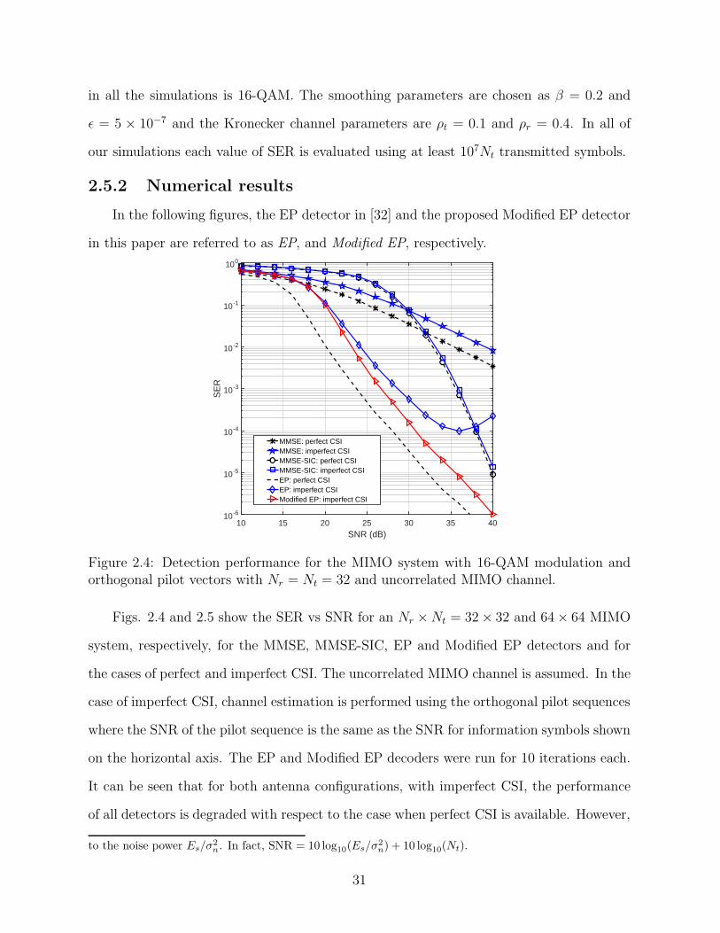
Figure 2.4: Detection performance for the MIMO system with 16-QAM modulation andorthogonal pilot vectors with Nr = Nt = 32 and uncorrelated MIMO channel.
Figs. 2.4 and 2.5 show the SER vs SNR for an Nr ×Nt = 32× 32 and 64× 64 MIMO
system, respectively, for the MMSE, MMSE-SIC, EP and Modified EP detectors and for
the cases of perfect and imperfect CSI. The uncorrelated MIMO channel is assumed. In the
case of imperfect CSI, channel estimation is performed using the orthogonal pilot sequences
where the SNR of the pilot sequence is the same as the SNR for information symbols shown
on the horizontal axis. The EP and Modified EP decoders were run for 10 iterations each.
It can be seen that for both antenna configurations, with imperfect CSI, the performance
of all detectors is degraded with respect to the case when perfect CSI is available. However,
to the noise power Es/σ2
n. In fact, SNR = 10 log10(Es/σ
2
n) + 10 log10(Nt).
31

10 15 20 25 30 35 40SNR (dB)
10-6
10-5
10-4
10-3
10-2
10-1
100
SE
R
MMSE: perfect CSIMMSE: imperfect CSIMMSE-SIC: perfect CSIMMSE-SIC: imperfect CSIEP: perfect CSIEP: imperfect CSIModified EP: imperfect CSI
Figure 2.5: Detection performance for the MIMO system with 16-QAM modulation andorthogonal pilot vectors with Nr = Nt = 64 and uncorrelated MIMO channel..
the results also show that the EP algorithm is much more sensitive to the CSI errors than
MMSE and MMSE-SIC.
Examining the covariance matrix of the total error given in (2.17), we find that at low
SNR values the noise plays a dominant role over the CSI estimation errors. Therefore, as
Figs 2.4 and 2.5 show, at very low SNR values the SER performances of EP and Modified
EP detectors are close. However, as SNR increases, the term in (2.17) related to channel
estimation error becomes more dominant. In this case, without compensating for the effect
of channel estimation errors, the EP algorithm does not converge to the correct symbol
values. This deteriorates the SER performance such that for higher SNR values, the SER
curves reach a plateau or even start to rise. On the other hand, these results also show
that the slope of the SER vs. SNR plots for the Modified EP detector with imperfect CSI
is similar to that of the EP detector with perfect CSI, and that the Modified EP detector
provides a much better performance at higher SNR values. For example, Fig. 2.4 shows
that for SER of 10−4, the Modified EP detector outperforms the EP detector by about 5
dB. Moreover, at SNR= 36 dB, the performance of EP starts to deteriorate.
32
As discussed previously, Fig. 2.3(b) provides an intuitive explanation for the perfor-
mance improvements of the Modified EP detector. As shown in this figure, the Modified
EP detector aligns its search area to the direction of the estimation error by employing the
proper error covariance matrix Rw and, as a result performs significantly better at higher
SNR values.
Figs. 2.6, 2.7 and 2.8 show the SER vs SNR for an Nr × Nt = 12 × 12, 20 × 20,
and 32 × 32 MIMO system, respectively, for the MMSE, MMSE-SIC, EP and Modified
EP detectors and for the cases of perfect and imperfect CSI, where the Kronecker channel
model is assumed. Channel estimation in the case of imperfect CSI is the same as in Figs.
2.4 and 2.5. The EP and Modified EP decoders were run for 10 iterations each. It can be
seen that as in the case of uncorrelated channels, the EP algorithm is much more sensitive
to CSI errors than MMSE and MMSE-SIC.
10 15 20 25 30 35 40SNR (dB)
10-6
10-5
10-4
10-3
10-2
10-1
100
SE
R
MMSE: perfect CSIMMSE: imperfect CSIMMSE-SIC: perfect CSIMMSE-SIC: imperfect CSIEP: perfect CSIEP: imperfect CSIModified EP: imperfect CSI
Figure 2.6: Detection performance for the MIMO system with 16-QAM modulation andorthogonal pilot vectors with Nr = Nt = 12 over the correlated channel.
Comparing the results in Figs. 2.6-2.8 reveals that the sensitivity of the EP algorithm
to channel estimation errors increases for larger antenna arrays. It can be seen that for
this correlated channel model, again the proposed modified EP detector helps recover a
33
10 15 20 25 30 35 40SNR (dB)
10-6
10-5
10-4
10-3
10-2
10-1
100
SE
R
MMSE: perfect CSIMMSE: imperfect CSIMMSE-SIC: perfect CSIMMSE-SIC: imperfect CSIEP: perfect CSIEP: imperfect CSIModified EP: imperfect CSI
Figure 2.7: Detection performance for the MIMO system with 16-QAM modulation andorthogonal pilot vectors with Nr = Nt = 20 over the correlated channel.
great deal of performance loss of the EP detector. For example, Fig. 2.7 shows that for
Nr = Nt = 20 and SER of 3×10⁻⁴, the Modified EP detector outperforms the EP detector
by about 5 dB. Moreover, the improvements are larger at higher SNR values.
Fig. 2.9 shows the performances of MMSE, MMSE-SIC, EP and Modified EP in the
case of imperfect CSI for an 80 × 80 MIMO system and the Kronecker channel model.
As indicated in the figure, the EP and Modified EP algorithms are evaluated for 2 and
4 iterations. This figure illustrates the effectiveness of the proposed method for large
scale systems. For example, for SER of 3 × 10⁻⁴, the proposed Modified EP algorithm
outperforms the EP algorithm by more than 3 dB.
It is interesting to note from Fig. 2.9 (as well as in some cases in the previous figures),
that the successive interference cancellation technique is not effective and the MMSE de-
coder outperforms MMSE-SIC decoder. The reason is that for the large value of Nt = 80,
and the given values of SNR in this figure, the ratio of Es/σ2n is small (e.g., for SNR=30 dB,
Es/σ2n = 10.97 dB), and for such small values of Es/σ
2n, successive interference cancellation
is not effective resulting in poor performance for MMSE-SIC.
34
10 15 20 25 30 35 40SNR (dB)
10-7
10-6
10-5
10-4
10-3
10-2
10-1
100
SE
R
MMSE: perfect CSIMMSE: imperfect CSIMMSE-SIC: perfect CSIMMSE-SIC: imperfect CSIEP: perfect CSIEP: imperfect CSIModified EP: imperfect CSI
Figure 2.8: Detection performance for the MIMO system with 16-QAM modulation andorthogonal pilot vectors with Nr = Nt = 32 over the correlated channel.
As discussed previously, orthogonal pilots result in the best MMSE estimation for un-
correlated channels. However, orthogonal codes are not available for arbitrary values of
Nt10. Using non-orthogonal pilot sequences increases the channel estimation error. There-
fore considering non-orthogonal pilots can also emulate the pilot contamination scenario
in massive MIMO systems which inevitably results in increased channel estimation error.
For the above reasons, in the next two simulations we assume semi-orthogonal pilot se-
quences which are generated using Gold sequences [43, 24]. As in the previous simulations,
we assume τ = Nt and the channel model is the same as that described in (2.37)-(2.38).
Channel estimation is performed using the pilot sequences as described in Section 2.4.2,
and the EP and Modified EP detectors are implemented using the estimated CSI. The EP
and Modified EP detectors are simulated with 4 iterations.
Fig. 2.10 shows the SER vs. SNR for the Nr×Nt = 32×25 and 100×25 MIMO system
10While OFDM-based wideband MIMO standards, such as LTE use temporal and frequency orthog-onality for pilots, here we assume the pilot symbols of all transmit antennas (or users) are transmittedsimultaneously in the same frequency band. In other words, orthogonality among the pilot sequences isprovided by codeword orthogonality. It is well known that such orthogonal codes (e.g., Walsh-Hadamardcodes) do not exist for arbitrary values of Nt [24].
35
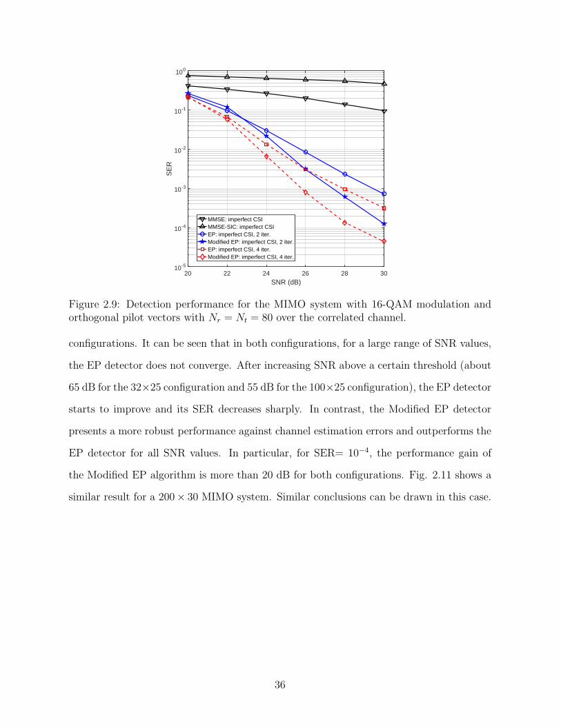
20 22 24 26 28 30SNR (dB)
10-5
10-4
10-3
10-2
10-1
100
SE
R
MMSE: imperfect CSIMMSE-SIC: imperfect CSIEP: imperfect CSI, 2 iter.Modified EP: imperfect CSI, 2 iter.EP: imperfect CSI, 4 iter.Modified EP: imperfect CSI, 4 iter.
Figure 2.9: Detection performance for the MIMO system with 16-QAM modulation andorthogonal pilot vectors with Nr = Nt = 80 over the correlated channel.
configurations. It can be seen that in both configurations, for a large range of SNR values,
the EP detector does not converge. After increasing SNR above a certain threshold (about
65 dB for the 32×25 configuration and 55 dB for the 100×25 configuration), the EP detector
starts to improve and its SER decreases sharply. In contrast, the Modified EP detector
presents a more robust performance against channel estimation errors and outperforms the
EP detector for all SNR values. In particular, for SER= 10−4, the performance gain of
the Modified EP algorithm is more than 20 dB for both configurations. Fig. 2.11 shows a
similar result for a 200× 30 MIMO system. Similar conclusions can be drawn in this case.
36
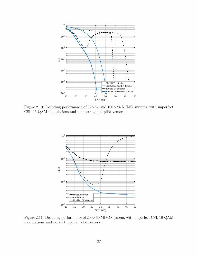
10 20 30 40 50 60 70 80SNR (dB)
10-6
10-5
10-4
10-3
10-2
10-1
100
SE
R
32x25 EP detector32x25 Modified EP detector100x25 EP detector100x25 Modified EP detector
Figure 2.10: Decoding performance of 32×25 and 100×25 MIMO systems, with imperfectCSI, 16-QAM modulations and non-orthogonal pilot vectors .
10 15 20 25 30 35 40 45 50SNR (dB)
10-3
10-2
10-1
100
SE
R
MMSE detectorEP detectorModified EP detector
Figure 2.11: Decoding performance of 200×30 MIMO system, with imperfect CSI, 16-QAMmodulations and non-orthogonal pilot vectors .
37
Chapter 3
Noncoherent SIMO Detection by
Expectation Propagation
3.1 Introduction
The advantages envisioned from using large antenna arrays have made massive multiple-
input multiple-output (MIMO) systems a promising technology for future wireless stan-
dards [9, 10]. Massive MIMO systems are expected to provide unprecedented gains in
spectral and energy efficiency along with low-complexity linear processing. One of the
roadblocks to achieving the promise of massive MIMO systems is the need for accurate
knowledge of channel state information (CSI) at the receiver for a large number of channels
[44]. Acquiring CSI through transmission of pilot sequences, as is common in many wireless
standards, is a resource-consuming task. Since the number of transmitters determines the
minimum length of the pilot sequence, increasing the number of antennas in massive MIMO
systems intensifies this issue. In particular, the required time for transmitting pilot symbols
over the forward link of a massive MIMO system may exceed the nominal coherence time
of the channel. Consequently, deployment of massive MIMO systems in frequency division
duplexing (FDD) mode is still an open problem [10]. Even in time division duplexing
(TDD) mode, due to lack of enough orthogonal sequences, pilots must be shared among
cells, giving rise to the so-called pilot contamination problem [9]. This challenge has mo-
tivated many researchers to investigate efficient noncoherent or pilotless symbol detection
algorithms.
Noncoherent techniques based on sphere decoding determine an efficient search radius
in order to reduce the detection complexity [45, 46]. However, sphere decoding based
algorithms still suffer from the well-known drawback of high complexity at low SNR values.
A noncoherent SIMO detection over uncorrelated Rician fading channel is proposed in [47].
The suggested algorithm is based on a proposed modulation technique in which information
38
is carried in the power of the transmitted symbols. Since the proposed method relies on
averaging the received power over all the receiving antennas, it may need unreasonably
large antenna arrays to achieve the desired performance. Therefore, the authors suggest
deploying a random code to improve detection performance for smaller antenna arrays [48].
Also, boundary regions in the suggested algorithm are determined by prior knowledge of
the channel statistics. As a result, the overall performance strongly depends on the quality
of prior knowledge about the Rician channel factor K and the noise power. In [49] the
authors propose an optimal constellation for achieving the minimum noncoherent detection
error, where the dependency on large scale channel statistics is reduced by applying proper
constellation design. Another algorithm in [50] proposes a noncoherent scheme for large
scale SIMO systems based on the knowledge of the average received powers from different
users. The authors present a specific constellation design such that the receiver can separate
the users.
In this paper we propose a noncoherent detection scheme for SIMO systems based on
the expectation propagation (EP) algorithm [38, 31]. The proposed EP detector iteratively
searches for the best approximation of the joint probability density function (pdf) of the
channel coefficients and the transmitted symbols. The output pdf is used for direct esti-
mation of the channel coefficients, as well as the transmitted symbols. We show that for
block fading channels, the proposed detector outperforms the pilot-based MMSE detector
for both Rayleigh and Rician channels (without prior knowledge of Rician channel factor),
for block sizes as small as two symbols. This makes this detector suitable for fast fad-
ing channels with very short coherence time. In addition, numerical results show that the
performance of this detector converges to that of the optimal maximum likelihood (ML) de-
tector with perfect channel state information (CSI), when the size of the transmitted block
increases. Finally, the proposed method does not rely on specific signal constellations and
can be used for any differential modulation scheme.
The rest of this chapter is organized as follows. The system model is presented in
39
Section 3.2. The proposed algorithm is presented in Section 3.3. Finally the simulation
results are presented in Sections 3.4.
Notations: Throughout this paper, small letters (x) are used for scalars, bold small
letters (x) for vectors, and capital letters (X) for matrices. R and C represent the set
of real and complex numbers, respectively. The superscripts (.)T , (.)H , and (.)−1 rep-
resent transpose, Hermitian transpose, and matrix inverse, respectively. Also, ⊗ de-
notes the matrix Kronecker product. For a complex-valued vector z = [z1, z2, · · · , zn]T ,
R(z) , [R(z1),R(z2), · · · ,R(zn)]T and I(z) , [I(z1), I(z2), · · · , I(zn)]T where R(zi) and
I(zi) denote the real and imaginary parts of the complex variable zi, respectively. For a
pdf p(.), Ep denotes the expectation operator with respect to p(.). IN denotes the N ×N
identity matrix. Finally, vec(A) and ||a|| denote the vectorization of the matrix A and the
ℓ2 norm of vector a, respectively.
3.2 System Model
Consider a SIMO system with Nr receiving antennas. The transmitted symbol at t-th
channel use, denoted by st, belongs to an M-ary modulation constellation AM with average
energy Es. The channel vector denoted by h ∈ CNr×1 is a circularly symmetric Gaussian
random vector with mean vector m0 and covariance matrix V0, i.e., h ∼ CN (h|m0, V0).
Note that for modeling the Rician fading channel with factor K, we can choose elements
of the mean vector such that |m0i|2 = K/(K + 1), and the covariance matrix as V0 =
1/(K + 1)INr.
We assume a narrowband block fading channel where h remains constant for the du-
ration of T transmitted symbols. The t-th received vector yt is given by
yt = sth+ wt (3.1)
where yt ∈ CNr×1, and wt ∼ CN (wt|0, σ2wINr
). To simplify notation, we consider the
40
all-real equivalent of (3.1) as follows
R(yt)
I(yt)
=
R(st) −I(st)
I(st) R(st)
⊗ INr
R(h)
I(h)
+
R(wt)
I(wt)
. (3.2)
Equivalently, this can be written as
yt = Sth+wt (3.3)
with yt ∈ R2Nr×1, h ∈ R2Nr×1, St ∈ R2Nr×2Nr , and finally wt ∈ R2Nr×1. For the new
channel vector h we have h ∼ p(h) = N (h|m0, V0), where m0 = [R(m0)TI(m0)
T ]T and
V0 =12I2 ⊗ V0. Similarly, wt ∼ N (wt|0, 12σ2
wI2Nr).
Assume a block of T independent transmitted symbols denoted as s , [s1, . . . , sT ].
Using (3.3), the corresponding received vectors are given by Y , [y1 . . . yT ]. We are
interested in a noncoherent detector where the channel vector h is unknown and must be
estimated along with the transmitted symbols s. The posterior joint distribution of the
unknown vectors s and h is given by
p(s,h|Y ) ∝ p(s,h)p(Y |s,h)
∝(
p(h)
T∏
t=1
p(st)
)
T∏
t=1
p(yt|st,h) (3.4)
in which p(st) is the probability mass function (pmf) of the t-th transmitted symbol. Since
the matrix St only depends on the single symbol st, we have p(yt|st,h) = p(yt|St,h) =
N(
yt|Sth,12σ2wI2Nr
)
.
The optimum receiver finds the maximizer of (3.4), i.e.,
(s,h)∗ = argmaxs∈AT
M,h∈R2Nr
p(s,h|Y ) (3.5)
Due to the complexity of (3.4), finding the optimum solution is generally very difficult and
41
requires multidimensional integration. The proposed EP algorithm in the next section ex-
ploits the multiplicative nature of (3.4) to find a simpler approximation for the conditional
joint distribution of (s,h) such that the marginals can be calculated with much less effort.
3.3 EP formulation for noncoherent detection
Let F denote a family of exponential distributions. Using EP we exploit the factorized
structure of (3.4) to approximate the posterior distribution p(s,h|Y ) with distributions
from F (for a review of the EP algorithm please refer to [51]). To this end we propose the
following approximation for p(s,h|Y ),
q′(s,h) ∝(
p(h)
T∏
t=1
p(st)
)
q(s,h) (3.6)
in which q(s,h) ∈ F may be considered as the approximation to the likelihood function
p(Y |s,h). As such, q(s,h) can be used for maximum likelihood estimation. However, the
receiver can use the prior pdfs to perform a Bayesian estimation from (3.6). Therefore,
we only need to apply the EP algorithm to the likelihood pdf of the received vectors.
We also note that since the channel vector is continuous and the transmitted symbols are
discrete, this will be a hybrid model [51]. The proposed approximation q(s, h) can be
further factorized as
q(s,h) ∝T∏
t=1
qt(st,h) ∝T∏
t=1
qt(st)qt(h) ∝ q(h)q(s) (3.7)
in which, qt(st,h) ∝ qt(st)qt(h), q(h) ∝∏T
t=1 qt(h) and q(s) =∏T
t=1 qt(st). We note that if
we select each factor qt(h) from F , then q(h) ∈ F , and consequently, q(s,h) ∈ F .
We assume that all qt(h) factors are multivariate Gaussian pdfs, i.e.,
qt(h) = N(
h|mh(t), Vh(t))
. (3.8)
42
Therefore q(h) = N (h|mh, Vh), where
Vh =
(
T∑
t=1
Vh(t)−1
)−1
(3.9)
and
mh = Vh
T∑
t=1
Vh(t)−1mh(t). (3.10)
Also, each qt(st) factor is assumed to be the pmf of its corresponding random symbol st.
Considering the M-ary modulation constellation AM = {a1, . . . , aM}, the pmf for st is the
set of probabilities as follows
qt(st) ={
P[st = a1], . . . ,P[st = aM ]}
. (3.11)
We use the t-th factor in the likelihood function, i.e., p(st,h|yt), for refining the t-th
approximating distribution, qt(st,h). Toward this, the t-th cavity distribution is calculated
as q\t(s,h) ∝ q(s,h)/qt(st,h) ∝ q\t(h)q\t(s), where q\t(h) ∝ q(h)/qt(h) and q\t(s) =
q(s)/qt(st) =∏T
i=1,i 6=t qi(si). It can be shown that q\t(h) ∝ N (h|m\th , V
\th ), where
V\th = (V −1
h − Vh(t)−1)−1 (3.12)
m\th = V
\th (V −1
h mh − Vh(t)−1mh(t)) (3.13)
Next, by combining the t-th factor of p(Y |s,h), given in (3.4), and the corresponding cavity
distribution, we compute the following intermediate pdf
pt(s,h) =1
Ztq\t(s,h)p(yt|st,h), (3.14)
43
where Zt = Eq\t(s,h)[p(yt|st,h)] is the normalization constant and can be calculated as
Zt =∑
st∈AM
N(
yt|Stm\th , StV
\th S
Tt +
1
2σ2wI2Nr
)
(3.15)
Since pt(s,h) is not a member of the exponential family, it is replaced with the closest
distribution in F , denoted as qnew(s,h) = qnew(h)qnew(s), where closeness is in the sense
of Kullback-Leibler (K-L) divergence. Therefore,
qnew(s,h) = argminq(s,h)∈ F
KL(
pt(s,h)||q(s,h))
(3.16)
It can be verified that the above optimization problem can be replaced with,
qnew(h) = argminq(h)∈ F
KL(
pt(h)||q(h))
(3.17)
and,
qnew(s) = argminq(s)
KL(
pt(s)||q(s))
(3.18)
where pt(s) and pt(h) are the respective marginal distributions of s and h, derived from
their joint distribution pt(s,h). In the following we will solve (3.17) and (3.18) separately
and use the solutions for updating the distributions of the corresponding factors.
Calculating qnew(h) and updating qt(h)
The marginal distribution of h is given by
pt(h) =∑
s∈ATM
pt(s,h) =1
Ztq\t(h)ψt(h) (3.19)
where ψt(h) ,∑
st∈AMp(yt|st,h), and the normalization constant Zt = Eq\t(h)[ψt(h)]. Ob-
viously, calculating Zt by this formula will give us the same result as in (3.15). The interme-
diate distribution pt(h) should be approximated by a pdf of the form q(h) = N (h|mh, Vh)
44
which satisfies (3.17). It turns out that the solution is obtained from the so-called moment
matching condition [38], resulting in the new moments of q(h) given by
mnewh = m
\th + V
\th ∇m (3.20)
and,
V newh = V
\th − V
\th (∇m∇T
m − 2∇v)V\th (3.21)
where, ∇m and∇v are gradients defined as∇m ,
(
∂ logZt/∂m\th
)T
and∇v ,
(
∂ logZt/∂V\th
)T
,
respectively. Using (3.15), it can be shown that (the proofs are omitted because of space
limitation)
∇m =1
Zt
∑
st∈AM
[
N(
yt|Stm\th ,Σt
)
STt Σ
−1t ζt
]
(3.22)
and,
∇v =1
2Zt
∑
st∈AM
[
N(
yt|Stm\th ,Σt
)
×
(
STt Σ
−1t ζtζ
Tt Σ
−1t St − ST
t Σ−1t St
)
]
(3.23)
where, ζt = yt − Stm\th and
Σt = StV\th S
Tt +
1
2σ2wI2Nr
. (3.24)
After updating q(h), its t-th factor qt(h), as in (3.8), is obtained from qnewt (h) ∝
qnew(h)/q\t(h). Therefore, the new values for mh(t) and Vh(t) are given by
V newh (t) =
(
(
V newh
)−1 −(
V\th
)−1
)−1
(3.25)
and,
mnewh (t) = V new
h (t)
(
(
V newh
)−1mnew
h −(
V\th
)−1m
\th
)
. (3.26)
45
Note that these updates do not depend on a specific value of the transmitted symbol st, and
in fact a form of averaging over all possible values of this symbol appears in the formulas.
Calculating qnew(s) and updating qt(st)
The marginal distribution of s is given by
pt(s) =
∫
h
pt(s,h)dh =1
Ztq\t(s)N
(
yt|Stm\th ,Σt
)
(3.27)
in which, Σt is given by (3.24). Therefore, the K-L divergence in (3.18) can be written as
KL(pt(s)||q(s)) =∑
s∈ATM
pt(s) logpt(s)
q(s)(3.28)
=∑
st∈AM
N(
yt|Stm\th ,Σt
)
Zt
× log
N
(
yt|Stm\th,Σt
)
Zt
qt(st)(3.29)
The minimizer of (3.29) for every st ∈ AM and t = 1, . . . , T is given by
qnewt (st) =1
Zt
N(
yt|Stm\th ,Σt
)
(3.30)
Note that solving (3.18) only updates the pmf of the t-th symbol, namely qt(st).
Each EP iteration involves updating all the T factors of qt(h) by (3.20) and (3.21)
and qnewt (st) in (3.30). After the EP algorithm converges, mh is adopted as the Maximum
likelihood (ML) estimate of the unknown channel, i.e, h′ = mh. Consequently, the channel
vector in (3.1) is given by
h′= mh,1:Nr
+ jmh,Nr+1:2Nr. (3.31)
Also, the following ML detection rule is employed for the transmitted symbols
s′t = argmaxa∈AM
qt(a), t = 1, . . . , T. (3.32)
46
As pointed out previously, the update rules for the moments of qt(h) in (3.25) and
(3.26) reveal that they are independent of the specific value of the symbol st. In other
words, refining the pdf factors for the channel is independent of refining the pdf factors for
the transmitted symbols. This is to be expected since the channel vector is constant over
all the received vectors1. Consequently, we do not need to updated the pmf of the symbols
at each iteration. In fact, calculations of (3.30) for all symbols may be postponed to the
end of the EP iterations, where the uncertainty about h is very small.
Now, at each iteration of the EP algorithm, the estimation of h gets closer to its actual
value. This implies that the mean of q(h) approaches the actual value of the channel vector
h and the elements of the covariance matrix of q(h) become smaller. Therefore, after an
adequate number of iterations, the factors qt(h) become almost identical and independent
of t. In other words, after a number of iterations, we will have mh(1) ≈ . . . ≈ mh(T ) and
Vh(1) ≈ . . . ≈ Vh(T ). Inserting these values into (3.9) and (3.10), we get mh = mh(1)
and Vh = Vh(1)/T . Then, from (3.12) and (3.13) we can write, m\th = mh and V
\th =
Vh(1)/(T − 1) ≈ Vh. Therefore, (3.30) can be calculated after the final iteration of EP
using these values of m\th and V
\th . Moreover, since after an adequate number of iterations,
the elements of V\th will become very small, we can further simplify the calculation of qt(st)
by replacing Vh with the all-zero matrix. Finally, for every st ∈ AM and t = 1, . . . , T , the
pmf of the transmitted symbols can be calculated from
qt(st) =N(
yt|Stmh,12σ2wI2Nr
)
∑
s′t∈AMN(
yt|S ′tmh,
12σ2wI2Nr
) (3.33)
Therefore, the ML detection rule of (3.32) reduces to
s′t = argminst∈AM
||yt − Stmh||2, t = 1, . . . , T. (3.34)
1Note that this may not be true in the case of fast fading channels where the channel vector maychange from symbol to symbol. In this case estimation of the channel coefficients at time t and detectionof the transmitted symbol at time t will be interconnected.
47
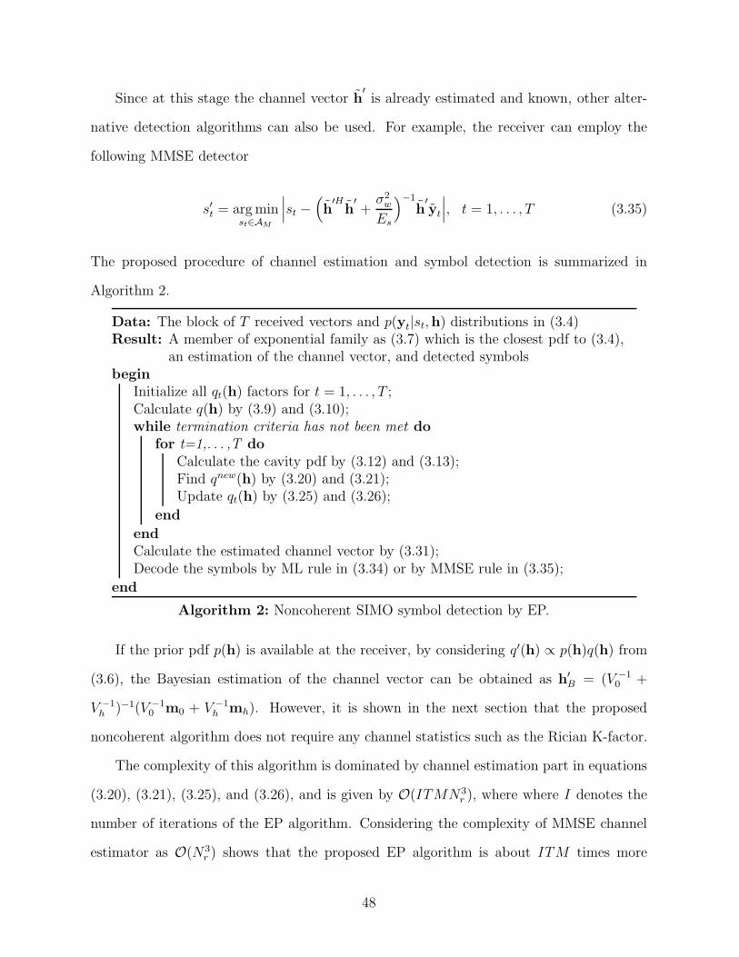
Since at this stage the channel vector h′is already estimated and known, other alter-
native detection algorithms can also be used. For example, the receiver can employ the
following MMSE detector
s′t = argminst∈AM
∣
∣
∣st −
(
h′Hh′+σ2w
Es
)−1
h′yt
∣
∣
∣, t = 1, . . . , T (3.35)
The proposed procedure of channel estimation and symbol detection is summarized in
Algorithm 2.
Data: The block of T received vectors and p(yt|st,h) distributions in (3.4)Result: A member of exponential family as (3.7) which is the closest pdf to (3.4),
an estimation of the channel vector, and detected symbolsbegin
Initialize all qt(h) factors for t = 1, . . . , T ;Calculate q(h) by (3.9) and (3.10);while termination criteria has not been met do
for t=1,. . . ,T do
Calculate the cavity pdf by (3.12) and (3.13);Find qnew(h) by (3.20) and (3.21);Update qt(h) by (3.25) and (3.26);
end
end
Calculate the estimated channel vector by (3.31);Decode the symbols by ML rule in (3.34) or by MMSE rule in (3.35);
end
Algorithm 2: Noncoherent SIMO symbol detection by EP.
If the prior pdf p(h) is available at the receiver, by considering q′(h) ∝ p(h)q(h) from
(3.6), the Bayesian estimation of the channel vector can be obtained as h′B = (V −1
0 +
V −1h )−1(V −1
0 m0 + V −1h mh). However, it is shown in the next section that the proposed
noncoherent algorithm does not require any channel statistics such as the Rician K-factor.
The complexity of this algorithm is dominated by channel estimation part in equations
(3.20), (3.21), (3.25), and (3.26), and is given by O(ITMN3r ), where where I denotes the
number of iterations of the EP algorithm. Considering the complexity of MMSE channel
estimator as O(N3r ) shows that the proposed EP algorithm is about ITM times more
48
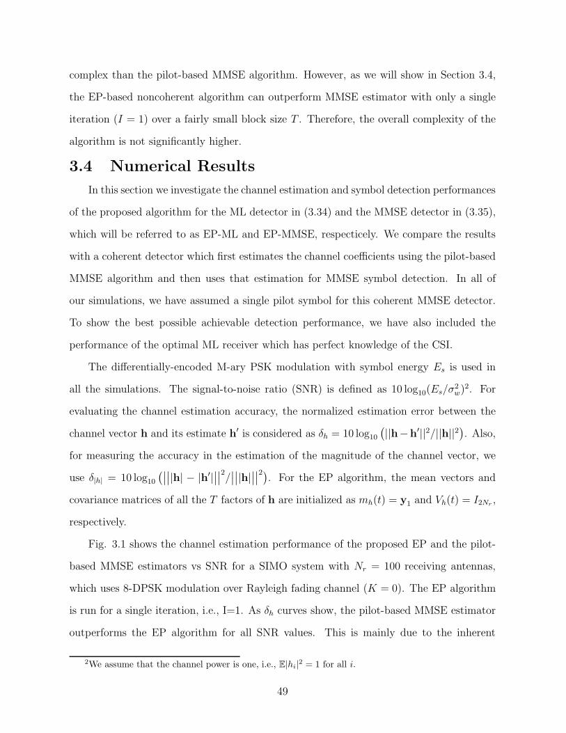
complex than the pilot-based MMSE algorithm. However, as we will show in Section 3.4,
the EP-based noncoherent algorithm can outperform MMSE estimator with only a single
iteration (I = 1) over a fairly small block size T . Therefore, the overall complexity of the
algorithm is not significantly higher.
3.4 Numerical Results
In this section we investigate the channel estimation and symbol detection performances
of the proposed algorithm for the ML detector in (3.34) and the MMSE detector in (3.35),
which will be referred to as EP-ML and EP-MMSE, respecticely. We compare the results
with a coherent detector which first estimates the channel coefficients using the pilot-based
MMSE algorithm and then uses that estimation for MMSE symbol detection. In all of
our simulations, we have assumed a single pilot symbol for this coherent MMSE detector.
To show the best possible achievable detection performance, we have also included the
performance of the optimal ML receiver which has perfect knowledge of the CSI.
The differentially-encoded M-ary PSK modulation with symbol energy Es is used in
all the simulations. The signal-to-noise ratio (SNR) is defined as 10 log10(Es/σ2w)
2. For
evaluating the channel estimation accuracy, the normalized estimation error between the
channel vector h and its estimate h′ is considered as δh = 10 log10(
||h−h′||2/||h||2)
. Also,
for measuring the accuracy in the estimation of the magnitude of the channel vector, we
use δ|h| = 10 log10(∣
∣
∣
∣|h| − |h′|∣
∣
∣
∣
2/∣
∣
∣
∣|h|∣
∣
∣
∣
2). For the EP algorithm, the mean vectors and
covariance matrices of all the T factors of h are initialized as mh(t) = y1 and Vh(t) = I2Nr,
respectively.
Fig. 3.1 shows the channel estimation performance of the proposed EP and the pilot-
based MMSE estimators vs SNR for a SIMO system with Nr = 100 receiving antennas,
which uses 8-DPSK modulation over Rayleigh fading channel (K = 0). The EP algorithm
is run for a single iteration, i.e., I=1. As δh curves show, the pilot-based MMSE estimator
outperforms the EP algorithm for all SNR values. This is mainly due to the inherent
2We assume that the channel power is one, i.e., E|hi|2 = 1 for all i.
49
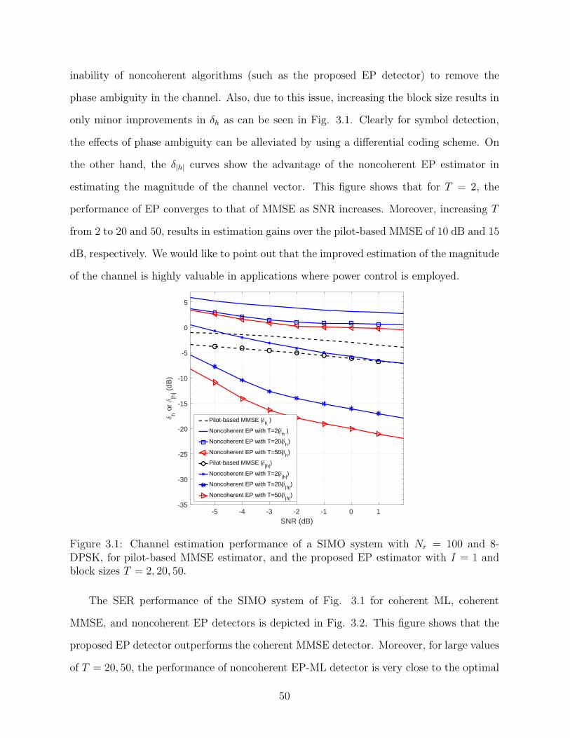
inability of noncoherent algorithms (such as the proposed EP detector) to remove the
phase ambiguity in the channel. Also, due to this issue, increasing the block size results in
only minor improvements in δh as can be seen in Fig. 3.1. Clearly for symbol detection,
the effects of phase ambiguity can be alleviated by using a differential coding scheme. On
the other hand, the δ|h| curves show the advantage of the noncoherent EP estimator in
estimating the magnitude of the channel vector. This figure shows that for T = 2, the
performance of EP converges to that of MMSE as SNR increases. Moreover, increasing T
from 2 to 20 and 50, results in estimation gains over the pilot-based MMSE of 10 dB and 15
dB, respectively. We would like to point out that the improved estimation of the magnitude
of the channel is highly valuable in applications where power control is employed.
-5 -4 -3 -2 -1 0 1SNR (dB)
-35
-30
-25
-20
-15
-10
-5
0
5
δh o
r δ
|h| (
dB)
Pilot-based MMSE (δh )
Noncoherent EP with T=2(δh )
Noncoherent EP with T=20(δh)
Noncoherent EP with T=50(δh)
Pilot-based MMSE (δ|h|
)
Noncoherent EP with T=2(δ|h|
)
Noncoherent EP with T=20(δ|h|
)
Noncoherent EP with T=50(δ|h|
)
Figure 3.1: Channel estimation performance of a SIMO system with Nr = 100 and 8-DPSK, for pilot-based MMSE estimator, and the proposed EP estimator with I = 1 andblock sizes T = 2, 20, 50.
The SER performance of the SIMO system of Fig. 3.1 for coherent ML, coherent
MMSE, and noncoherent EP detectors is depicted in Fig. 3.2. This figure shows that the
proposed EP detector outperforms the coherent MMSE detector. Moreover, for large values
of T = 20, 50, the performance of noncoherent EP-ML detector is very close to the optimal
50
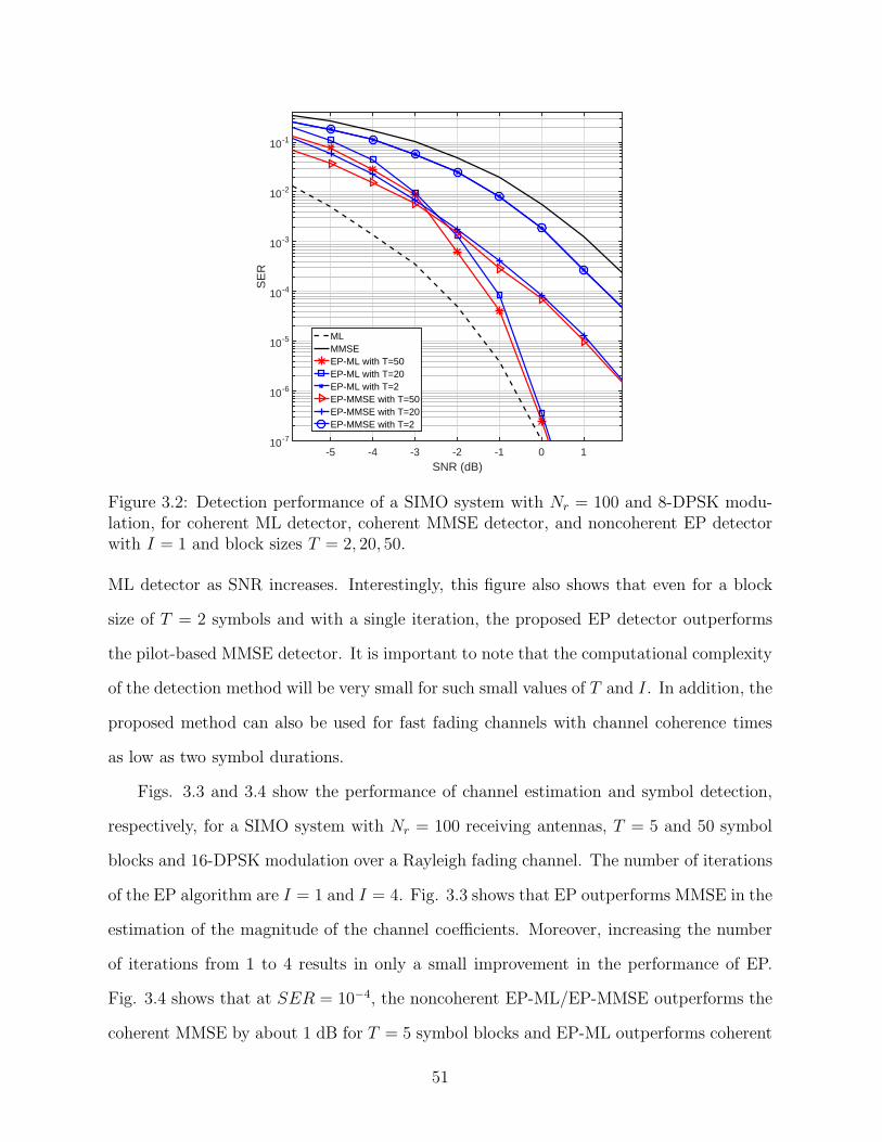
-5 -4 -3 -2 -1 0 1SNR (dB)
10-7
10-6
10-5
10-4
10-3
10-2
10-1
SE
R
MLMMSEEP-ML with T=50EP-ML with T=20EP-ML with T=2EP-MMSE with T=50EP-MMSE with T=20EP-MMSE with T=2
Figure 3.2: Detection performance of a SIMO system with Nr = 100 and 8-DPSK modu-lation, for coherent ML detector, coherent MMSE detector, and noncoherent EP detectorwith I = 1 and block sizes T = 2, 20, 50.
ML detector as SNR increases. Interestingly, this figure also shows that even for a block
size of T = 2 symbols and with a single iteration, the proposed EP detector outperforms
the pilot-based MMSE detector. It is important to note that the computational complexity
of the detection method will be very small for such small values of T and I. In addition, the
proposed method can also be used for fast fading channels with channel coherence times
as low as two symbol durations.
Figs. 3.3 and 3.4 show the performance of channel estimation and symbol detection,
respectively, for a SIMO system with Nr = 100 receiving antennas, T = 5 and 50 symbol
blocks and 16-DPSK modulation over a Rayleigh fading channel. The number of iterations
of the EP algorithm are I = 1 and I = 4. Fig. 3.3 shows that EP outperforms MMSE in the
estimation of the magnitude of the channel coefficients. Moreover, increasing the number
of iterations from 1 to 4 results in only a small improvement in the performance of EP.
Fig. 3.4 shows that at SER = 10−4, the noncoherent EP-ML/EP-MMSE outperforms the
coherent MMSE by about 1 dB for T = 5 symbol blocks and EP-ML outperforms coherent
51
MMSE by about 3 dB for T = 50. This figure also shows that by increasing the size of
the blocks to 50 symbols, SER performance of EP-ML converges to that of the optimal
ML receiver. Comparing the SER curves of the two EP detectors reveals that increasing T
results in only a small improvement in the performance of EP-MMSE. As before, increasing
the number of iterations has a negligible effect on the SER performance.
Fig. 3.5 shows the SER performance of three SIMO configurations with Nr = 10, 30,
and 60 antennas which use the proposed EP detector over a Rician fading channel with a
Rician factor of K = 10. Blocks of length T = 5 with 8-DPSK modulation are considered.
Also all EP algorithms are assumed to work with I = 1 iteration and without any prior
knowledge of K. This figure shows that for all configurations the proposed noncoherent
algorithm outperforms the coherent MMSE detector.
0 1 2 3 4 5 6SNR (dB)
-50
-45
-40
-35
-30
-25
-20
-15
-10
-5
0
5
δh (
dB)
or δ
|h| (
dB)
Pilot-based MMSE (δh )
Noncoherent EP, T=5, I=1(δh )
Noncoherent EP, T=5, I=4(δh)
Noncoherent EP, T=50, I=1(δh )
Noncoherent EP, T=50, I=4(δh)
Pilot-based MMSE (δ|h|
)
Noncoherent EP, T=5, I=1(δ|h|
)
Noncoherent EP, T=5, I=4(δ|h|
)
Noncoherent EP, T=50, I=1(δ|h|
)
Noncoherent EP, T=50, I=4(δ|h|
)
Figure 3.3: Channel estimation performance of a SIMO system with Nr = 100 and 16-DPSK modulation, for MMSE estimator with a single-symbol pilot, and EP estimatorswith block sizes T = 5, 50 and two different iterations I = 1 and I = 4.
52
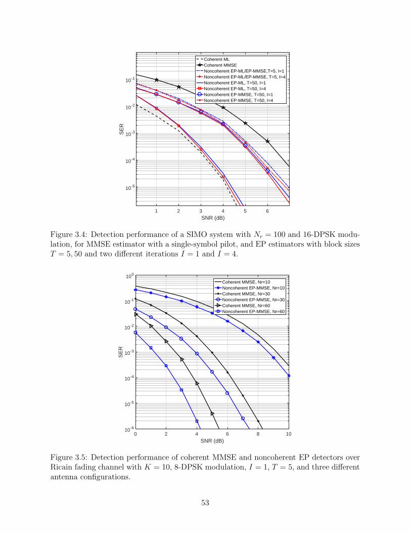
1 2 3 4 5 6SNR (dB)
10-5
10-4
10-3
10-2
10-1
SE
R
Coherent MLCoherent MMSENoncoherent EP-ML/EP-MMSE,T=5, I=1Noncoherent EP-ML/EP-MMSE, T=5, I=4Noncoherent EP-ML, T=50, I=1Noncoherent EP-ML, T=50, I=4Noncoherent EP-MMSE, T=50, I=1Noncoherent EP-MMSE, T=50, I=4
Figure 3.4: Detection performance of a SIMO system with Nr = 100 and 16-DPSK modu-lation, for MMSE estimator with a single-symbol pilot, and EP estimators with block sizesT = 5, 50 and two different iterations I = 1 and I = 4.
0 2 4 6 8 10SNR (dB)
10-6
10-5
10-4
10-3
10-2
10-1
100
SE
R
Coherent MMSE, Nr=10Noncoherent EP-MMSE, Nr=10Coherent MMSE, Nr=30Noncoherent EP-MMSE, Nr=30Coherent MMSE, Nr=60Noncoherent EP-MMSE, Nr=60
Figure 3.5: Detection performance of coherent MMSE and noncoherent EP detectors overRicain fading channel with K = 10, 8-DPSK modulation, I = 1, T = 5, and three differentantenna configurations.
53
Chapter 4
Joint Channel Estimation and
Symbol Detection for Multi-Cell
Massive MIMO Using Expectation
Propagation
4.1 Introduction
Since the gains offered by multiple-input multiple-output (MIMO) systems scale with
the number of transmitting and receiving antennas, research on high-order MIMO (also
referred to as massive MIMO) systems has been accelerating in recent years [8, 9, 10, 11].
Massive MIMO is a multi-user MIMO (MU-MIMO) system in which the base station (BS) is
equipped with an order-of-magnitude larger number of antennas compared to the traditional
MIMO systems. Early studies have demonstrated the benefits of massive MIMO systems
[12], and some field trials have been carried out to show the possibilities and limitations of
this technology [13, 14, 15].
In order to realize the potential advantages of massive MIMO systems, several technical
challenge must be addressed. Chief among them is the fact that symbol detection in
the receiver requires accurate knowledge of channel state information (CSI) for a large
number of channels [44]. Acquiring the CSI through transmission of pilot sequences, as is
common in many wireless standards, is a resource-intensive process, due to the large number
of channels involved. Moreover, since the number of transmitter antennas determines
the minimum length of the pilot sequence, increasing the number of antennas in massive
MIMO systems increases the length of pilot sequences. In particular, the required time
for transmitting pilot symbols over the forward link may exceed the nominal coherence
time of the channel. Consequently, deployment of massive MIMO systems in frequency
division duplexing (FDD) mode remains an open problem [11]. Even in time division
54
duplexing (TDD) mode, due to lack of enough orthogonal sequences, pilots must be shared
among the cells, giving rise to the so-called pilot contamination problem [9, 52]. This
has motivated many researchers to investigate efficient noncoherent or pilotless symbol
detection algorithms which do not require pilot transmission for CSI acquisition.
Noncoherent detection for single-input multiple-output (SIMO) systems is suggested
in several previous works. For instance, [45] and [46] propose techniques based on sphere
decoding with an efficient search radius. Another noncoherent technique based on a pro-
posed modulation technique in which information is carried in the power of the transmitted
symbols over uncorrelated Rician fading channel, is suggested in [47] and [48]. In [49] the
authors propose an optimal constellation for achieving the minimum noncoherent detection
error, where the dependency on large scale channel statistics is reduced by applying proper
constellation design. Another algorithm in [50] proposes a noncoherent scheme for large
scale SIMO systems based on the knowledge of the average received powers from different
users. In [53] we have developed a joint channel estimation and symbol detection algorithm
for SIMO systems based on Expectation Propagation (EP). It is shown in this work that
the proposed detector outperforms the pilot-based MMSE detector for both Rayleigh and
Rician fading channels.
When the ratio of the number of transmitting antennas to the number of receiving
antennas is small, as is common in the forward link of massive MIMO systems, there
will be a large degree of freedom which can be exploited by noncoherent algorithms. For
example, [54] suggests a noncoherent channel estimation technique for multi-cell massive
MIMO systems based on the eigenvalue decomposition (EVD) of the correlation matrix
of the received vectors. However, the proposed algorithm is sensitive to the size of the
antenna array as well as the accuracy of the empirically calculated correlation matrix of
the received vectors. A noncoherent algorithm based on subspace projection and random
matrix theory is suggested in [55, 56, 57]. Assuming that the number of users per cell
remains fixed, the authors show that under certain conditions on the powers of the trans-
55
mitting users, the spectrum of the sample covariance matrix asymptotically decomposes
into the signal eigenvalue spectrum and the interference-plus-noise eigenvalue spectrum as
the number of BS antennas grows [56]. The limiting support of the two spectra are approx-
imately characterized and a bound on the power difference of the signal and interference
is determined in order for the two to become disjoint. It is noted in [58] that this bound
is independent of the noise variance and, as a result, becomes inaccurate under low signal-
to-noise ratio (SNR) regime. A new asymptotic condition on spectrum separability is then
derived in [58] by considering the exact asymptotic characterization of interference-plus-
noise spectrum. These algorithms reduce pilot contamination by appropriate power control
and estimate the channel matrix of the desired cell. Finally [59] exploits the sparsity of
the massive MIMO channels and transforms the channel estimation problem into learning
on a Gaussian mixture model, which can be solved using algorithms such as Expectation
Maximization.
Coherent MIMO detection based on EP was recently suggested in [32], where the per-
formance of the algorithm is evaluated on the premise that perfect channel state information
(CSI) is available at the receiver. However, as mentioned earlier, providing perfect CSI in
massive MIMO systems is a challenging problem. At best, only a noisy estimate of the
channel coefficients will be available at the receiver. Also, other detrimental effects, such as
pilot contamination, aging and quantization errors, limit the accuracy of the CSI estimates.
In [60] we show that although channel estimation improves by increasing the signal-to-noise
ratio (SNR)1, surprisingly, at high SNR values, the rate of improvement of symbol error
rate (SER) vs. SNR decreases. We investigate this behavior of the EP detector in the case
of imperfect CSI and propose a modified detector in order to recover some of the perfor-
mance loss of the EP detector. Simulation results verify that the proposed modification
improves the performance of EP in the case of imperfect CSI, particularly in higher SNR
regions, and that for the modified detector, the slope of the SER vs. SNR plots are similar
1The SNR of the pilot and information sequences are assumed to be the same
56

to the case of perfect CSI.
In this work we propose a noncoherent channel estimation and symbol detection tech-
nique for multi-cell massive MIMO systems based on the Expectation Propagation (EP)
algorithm [38, 31]. Since the channel matrix and the transmitted vectors are both un-
known, the proposed EP-based algorithm is applied on a hybrid model [51], and iteratively
searches for the best approximation of the joint probability density function (PDF) of these
unknowns. The output PDF is used for direct estimation of the channel coefficients, as well
as the transmitted symbols. To overcome the inherent ambiguity of noncoherent estimators,
we use the output of the EVD-based estimator in [54] to initialize the channel coefficients
in our algorithm. This allows for the EP-based receiver to improve its performance over the
EVD-based algorithm. We show that the proposed EP estimator outperforms the EVD-
based algorithm in both channel estimation and symbol detection. Moreover, this approach
diminishes the sensitivity of the EVD-based algorithm to the array and transmission block
sizes.
The rest of this chapter is organized as follows. The system model is presented in
Section 4.2. Section 4.3 covers a brief review of the EVD-based algorithm. The proposed
algorithm is presented in Section 4.4. Finally, simulation results are presented in Section
4.5.
Notations: Throughout this paper, small letters (x) are used for scalars, bold small
letters (x) for vectors, and capital letters (X) for matrices. R and C represent the set
of real and complex numbers, respectively. R(z) and I(z) denote the real and imaginary
parts of the complex variable z. For a set of complex variables A = {z1, z2, · · · }, we
denote R(A) , {R(z1),R(z2), · · · } and I(A) , {I(z1), I(z2), · · · }. The superscripts (.)T ,
(.)H , and (.)−1 represent transpose, Hermitian transpose, and matrix inverse, respectively.
Also, ⊗ and ◦ denote the matrix Kronecker and Hadamard products, respectively. For a
probability density function (PDF) p(.), Ep denotes the expectation operator with respect
to p(.). IN denotes the N × N identity matrix and diag[λ1, λ2, . . . , λn] denotes the n × n
57
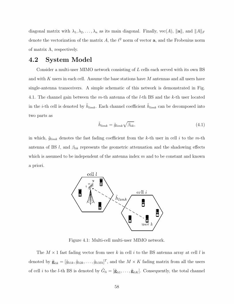
diagonal matrix with λ1, λ2, . . . , λn as its main diagonal. Finally, vec(A), ‖a‖, and ‖A‖Fdenote the vectorization of the matrix A, the ℓ2 norm of vector a, and the Frobenius norm
of matrix A, respectively.
4.2 System Model
Consider a multi-user MIMO network consisting of L cells each served with its own BS
and with K users in each cell. Assume the base stations haveM antennas and all users have
single-antenna transceivers. A simple schematic of this network is demonstrated in Fig.
4.1. The channel gain between the m-th antenna of the l-th BS and the k-th user located
in the i-th cell is denoted by hlimk. Each channel coefficient hlimk can be decomposed into
two parts as
hlimk = glimk
√
βlik, (4.1)
in which, glimk denotes the fast fading coefficient from the k-th user in cell i to the m-th
antenna of BS l, and βlik represents the geometric attenuation and the shadowing effects
which is assumed to be independent of the antenna index m and to be constant and known
a priori.
Figure 4.1: Multi-cell multi-user MIMO network.
The M × 1 fast fading vector from user k in cell i to the BS antenna array at cell l is
denoted by glik = [gli1k, gli2k, . . . , gliMk]T , and the M ×K fading matrix from all the users
of cell i to the l-th BS is denoted by Gli = [gli1, . . . , gliK ]. Consequently, the total channel
58
gain between users in cell i and the BS in cell l will be an M ×K matrix denoted by Hli
and given by
Hli , GliD1
2
li (4.2)
where Dli , diag[βli1, βli2, . . . , βliK ].
Assuming that the fast fading coefficients between different channels and/or users are
independent and identically distributed (iid) with E[glimkg∗l′i′m′k′] = δll′δii′δmm′δkk′, we get
E[GliGHlj ] = KIMδij . Therefore,
E[HliHHlj ] = E[HliH
Hli ]δij = E[GliDliG
Hli ]δij (4.3)
=K∑
k=1
βlikE[glikgHlik]δij =
(
K∑
k=1
βlik
)
IMδij (4.4)
Without loss of generality, suppose we are interested in the first cell, i.e., l = 1. There-
fore, the received vector at this BS at t-th channel use is given by
y1(t) =L∑
i=1
H1isi(t) + w1(t) (4.5)
=H11s1(t) +
L∑
i=2
H1isi(t) + w1(t) (4.6)
where si(t) = [si1(t), si2(t), . . . , siK(t)]T is the vector of transmitted symbols by users in cell
i. The symbols sij(t) are assumed to be independently selected from an M-ary modulation
constellation denoted as AM, with zero mean and average energy Es. Therefore we have
E[
si(t)sj(t)H]
= EsδijIK . Also, wl(t) ∼ CN (wl|0, IM) is the circularly symmetric additive
white Gaussian noise at the l-th BS and are assumed to be independent for different BS’s.
Setting w′1(t) ,
∑Li=2 H1isi(t) + w1(t) as the combination of interference plus noise at BS
1, we can write
y1(t) = H11s1(t) + w′1(t) (4.7)
59

We can treat w′1(t) as a new additive noise vector. The mean of w′
1(t) is given by E[w′1(t)] =
0 and its covariance matrix can be calculated as follows.
R′w ,E[w′
1(t)(
w′1(t))H
] (4.8)
=
L∑
i=2
L∑
j=2
E
[
H1iE[
si(t)sj(t)H]
HH1j
]
+ IM (4.9)
=Es
L∑
i=2
E
[
H1iHH1i
]
+ IM (4.10)
=Es
L∑
i=2
(
K∑
k=1
β1ikIM
)
+ IM (4.11)
=(
Es
L∑
i=2
K∑
k=1
β1ik + 1)
IM (4.12)
Assuming that the product KL is large, we invoke the central limit theorem and assume
that the mulit-user interference∑L
i=2 H1isi(t) is a Gaussian random vector. It then follows
that the received vector at the first BS is given by (4.7), where w′1(t) ∼ CN
(
w′1|0, σ′2
wIM
)
,
and where
σ′2w , Es
L∑
i=2
K∑
k=1
β1ik + 1 (4.13)
To simplify our notations, for the received vector of the target BS in a multi-cell multi-user
model at t-th channel use, in the sequel we rewrite (4.7) as
yt = H st + w′t, (4.14)
in which, st ∈ AKM is the vector of transmitted symbols with entries in AM, H ∈ CM×K
is the channel matrix, and w′t ∈ CM×1 is the additive noise vector such that w′
t ∼
CN (w′t|0, σ′2
wIM) with σ′2w given in (4.13).
By applying the vectorization property vec(ABC) = (CT ⊗ A)vec(B), (4.14) can be
expressed as
yt = Sth+ w′t (4.15)
60
in which, St , sTt ⊗ IM and h , vec(H). The all-real equivalent of (4.15) is given by
R(yt)
I(yt)
=
R(St) −I(St)
I(St) R(St)
R(h)
I(h)
+
R(w′t)
I(w′t)
(4.16)
Denoting yt ,(
R(yTt ) I(y
Tt ))T
, St ,
R(St) −I(St)
I(St) R(St)
, h ,
(
R(hT) I(h
T))T
, and w′t ,
(
R(w′Tt ) I(w′T
t ))T
, (4.16) can be written as
yt = Sth+w′t. (4.17)
Finally it follows from the properties of circularly symmetric Gaussian random vectors that
w′t ∼ N (w′|0, 1
2σ′2wI2M).
For the noncoherent detector being considered here, the channel vector, h, as well as
the transmitted symbols, St, are unknown. Therefore, a joint symbol detection and channel
estimation algorithm must be employed at the receiver to estimate the channel vector and
detect the transmitted symbols.
Consider a block of T transmitted vectors S , [s1, . . . , sT ] and the corresponding re-
ceived vectors Y , [y1 . . . yT ]. We assume a block fading channel where the channel
matrices remain unchanged for the duration of a transmission block consisting of T trans-
mitted symbols. The posterior distribution of S and h is given by
p(S,h|Y ) ∝ p(S,h)p(Y |S,h)
∝(
p(h)T∏
t=1
p(st)
)
T∏
t=1
p(yt|st,h) (4.18)
in which p(st) is the probability mass function (pmf) of the t-th transmitted vector, p(h)
is the prior PDF of the channel vector,2 p(yt|st,h) is the a posteriori distribution of the
2In developing the noncoherent receiver, we assume that h is an unknown constant vector during the
61
t-th received vector, which from (4.17) is given by p(yt|st,h) = N(
yt|Sth,12σ′2wI2M
)
.3
The optimum receiver finds the unknowns as the maximizers of (4.18), namely,
(S,h)∗ = argmaxS∈AK×T
M ,h∈R2M
p(S,h|Y ) (4.19)
The optimization in (4.19) is not tractable due to the complexity of the posterior distribu-
tion in (4.18). In fact the optimization requires the computation of marginal distributions
which demand extensive multi-dimensional numerical integrations. In Section 4.4 we de-
velop an estimation technique based on the EP algorithm. This approach exploits the
multiplicative nature of (4.18) to find an approximation for the posterior distribution of
(S,h) so that the marginals can be easily computed.
4.3 Review of the EVD-Based Massive MIMO Chan-
nel Estimation
A channel estimation algorithm based on the existing degrees of freedom in massive
MIMO systems is suggested in [54]. The proposed algorithm estimates the channel vectors
from the eigenvectors of the sample correlation matrix of the received vectors at the BS.
Suppose that we are interested in estimating the channel matrix of the first cell in the
multi-user multi-cell network. The received vector at the first BS at time t is given by
(4.5). The correlation matrix of this vector is given by
Ry , E[y1(t)yH1 (t)]
= E[(
L∑
i=1
H1isi(t) + w1(t))(
L∑
j=1
H1j sj(t) + w1(t))H]
= Es
L∑
i=1
H1iHH1i + IM = Es
L∑
i=1
G1iD1iGH1i + IM (4.20)
observation period T . However, to estimate it using the EP algorithm, we estimate a PDF for h fromwhich the ML estimate of h is obtained.
3Note that the matrix St only depends on the vector st. Therefore, for the conditional PDF of yt wecan write p(yt|St,h) = p(yt|st,h).
62
Under the so-called favorable propagation condition, [9], the channel vectors of different
terminals will be mutually orthogonal, i.e., as M −→ ∞,
1
MGH
li Glj −→ IKδij (4.21)
Therefore, multiplying Ry by G11 and using (4.21) we get
RyG11 ≈ Es
L∑
i=1
G1iD1iGH1iG11 + G11
= G11(EsMD11 + IK). (4.22)
Note that Λ11 , EsMD11 + IK is a diagonal matrix with {EsMβ11k + 1, k = 1, . . . , K}
as its main diagonal. Therefore, RyG11 = G11Λ11 along with the pairwise orthogonality
of columns of G11 shows that (4.22) can be considered as the characteristic equation of
the correlation matrix Ry. Therefore, the kth column of G11 is proportional to the kth
eigenvector of Ry corresponding to the eigenvalue EsMβ11k+1. Assuming that EsMβ11k+1,
k = 1, 2, . . . , K are distinct and known a priori, the ordering of the eigenvectors among the
K users can be determined up to a constant factor. In other words, if U1 is the M × K
matrix whose columns are the eigenvectors of Ry, then the estimate of G11, denoted by G11
is given by G11 = U1C1, where C1 is a diagonal matrix. Since C1 is unknown at the BS, it
is estimated using a short pilot sequence.
Suppose each user transmits τ pilot symbols. Assuming that the pilots of different cells
are mutually orthogonal, the received M × τ matrix at the 1st BS is given by
Y1 = H11P1 + W1 (4.23)
where P1 is theK×τ matrix of pilots from the K users in cell 1, and W1 is the noise matrix.
The ambiguity matrix C1 can now be estimated by solving the following optimization
63
problem
C1 = argminC1∈Θ
‖Y1 − U1C1D1/211 P1‖2F , (4.24)
in which Θ is the set of all K ×K diagonal matrices in CK×K .
Denoting J , ‖Y1 − U1C1D1/211 P1|‖2F and considering the optimization constraint, the
derivative of J with respect to C1 is given by
∂J
∂C1= (D
1/211 P1P
H1 D
1/211 C
H1 U
H1 U1 −D
1/211 P1Y
H1 U1) ◦ IK (4.25)
Solving ∂J/∂C1 = 0 leads to
(ΞCH1 Φ) ◦ IK = Ψ ◦ IK , (4.26)
in which, Ξ = D1/211 P1P
H1 D
1/211 , Φ = UH
1 U1, and Ψ = D1/211 P1Y
H1 U1. Now, suppose the
vector of K diagonal elements of C1 is denoted by c1. Then, it can be easily shown that
the solution of (4.26) is
c1 = (ΦH ◦ Ξ∗)−1(Ψ ◦ IK)1K , (4.27)
in which, 1K is a K × 1 all-one vector.
After calculating the constant matrix, the channel can be estimated as
H11 = U1C1D1
2
11 (4.28)
In practice the correlation matrix Ry is not available and the sample covariance matrix
is used instead. Using a block ofN samples, the sample correlation matrix can be calculated
as
Ry =1
N
N∑
n=1
y1(n)yH1 (n) (4.29)
As mentioned in [54], error in the calculated sample correlation matrix due to the
64
limited block size N and lack of true channel mutual orthogonality, particularly for smaller
antenna arrays, are two major sources of error in the proposed algorithm. In this paper
we develop an EP-based noncoherent detector which is initialized with the output of the
EVD-based detector. After a few iterations, the proposed detector significantly improves
the performance of the EVD-based detector.
4.4 EP Formulation for Noncoherent Detection
Let F denote a family of exponential distributions. Using EP we exploit the factorized
structure of (4.18) to approximate the posterior distribution p(S,h|Y ) with distributions
from F (for a review of the EP algorithm please refer to [38, 31]). To this end, we employ
the following approximation for the posterior distribution p(S,h|Y ),
q′(S,h) =
(
p(h)
T∏
t=1
p(st)
)
q(S,h) (4.30)
in which q(S,h) ∈ F is considered as an approximation to the likelihood function p(Y |S,h).
Since the channel vector is a continuous vector and the transmitted symbols are discrete
random variables, this will be a hybrid model [51]. After calculating q(S,h) from EP as the
best approximation (in F) to p(Y |S,h), an approximation to the a posterior distribution
can be calculated using (4.30). However, assuming independent, identically distributed (iid)
transmitted vectors, the solution to (4.19) can be equivalently obtained from maximizing
the likelihood function p(Y |S,h). Therefore, we do not need to evaluate (4.30). The
transmitted vectors and channel coefficients can be estimated by maximizing q(S,h).
The proposed approximation q(S, h) is further written in a factorized form as follows.
q(S,h) ∝T∏
t=1
qt(st,h) ∝T∏
t=1
qt(st)qt(h) (4.31)
∝ q(S)q(h) (4.32)
in which, q(h) ∝∏Tt=1 qt(h) and q(S) =
∏Tt=1 qt(st). We note that by selecting each factor
65
qt(h) from F , we are ensured that their product, q(h), is also in F . Moreover, multiplying
q(h) by the pmf q(S) will not change its structure. Therefore q(S,h) will also be in the
family of exponential distributions.
We consider the family of multivariate Gaussian distributions for F . In particular,
we assume that all qt(h) factors are multivariate Gaussian with mean vector mh(t) and
covariance matrix Vh(t), i.e., qt(h) = N (h|mh(t), Vh(t)). Therefore their product will be
proportional to a multivariate Gaussian distribution q(h) = N (h|mh, Vh), with covariance
matrix
Vh =
(
T∑
t=1
Vh(t)−1
)−1
(4.33)
and mean vector
mh = Vh
T∑
t=1
Vh(t)−1mh(t). (4.34)
Also, all q(st) factors are assumed to be pmf of their corresponding random vectors. Since st
is aK-dimensional vector with elements from AM, for each possible vector st, q(st) will be a
set of MK probabilities. Denoting the set of all K-tuples over AM by A = {a1, . . . , aMK},
then q(st) can be defined as follows
q(st) =(
P[st = a1], . . . ,P[st = aMK ])
. (4.35)
EP uses the t-th factor in the likelihood function p(Y |S,h), i.e., p(yt|st,h), for refin-
ing the t-th approximating distribution qt(st,h). Toward this, the so called t-th cavity
distribution is calculated as
q\t(S,h) ∝ q(S,h)
qt(st,h)=
q(h)q(S)
qt(h)qt(st)(4.36)
∝ q\t(h)q\t(S) (4.37)
66

in which,
q\t(h) ∝ q(h)
qt(h)=
N (h|mh, Vh)
N (h|mh(t), Vh(t))(4.38)
∝ N (h|m\th , V
\th ) (4.39)
where it can be shown that
V\th = (V −1
h − Vh(t)−1)−1 (4.40)
m\th = V
\th
(
V −1h mh − Vh(t)
−1mh(t))
. (4.41)
Moreover,
q\t(S) ∝ q(S)
qt(st)=
∏Ti=1 qi(si)
qt(st)(4.42)
∝T∏
i=1i 6=t
qi(si) (4.43)
Combining the t-th factor in the likelihood function with the cavity distribution, we
compute the following intermediate distribution.
pt(S,h) =1
Zt
q\t(S,h)p(yt|st,h) (4.44)
where it is shown in Appendix F that the normalization constant Zt is given by
Zt =∑
st∈AKM
N(
yt|Stm\th ,Σt
)
(4.45)
where Σt , StV\th S
Tt + 1
2σ′2wI2M .
Since pt(S,h) is not a member of the exponential family, it should be mapped to the
67
closest distribution in F , denoted by qnew(S,h) = qnew(S)qnew(h), such that
qnew(S,h) = argminq(S,h)∈ F
KL(
pt(S,h)‖q(S,h))
(4.46)
= argminq(S,h)∈ F
KL(
pt(S,h)‖q(S)q(h))
. (4.47)
It is shown in Appendix G that the above optimization problem can be divided into the
following two separate optimizations:
qnew(h) = argminq(h)
KL(
pt(h)‖q(h))
, (4.48)
and
qnew(S) = argminq(S)
KL(
pt(S)‖q(S))
(4.49)
where pt(h) and pt(S) are the marginal distributions of h and S, respectively, derived from
their joint distribution pt(S,h).
In the following we solve the optimizations in (4.48) and (4.49) in that order. It turns
out that the solution of (4.48) is obtained from the so-called moment matching condition
[38], and (4.49) can be solved directly.
4.4.1 Calculation of qnew(h) and updating of qt(h)
The marginal distribution of h is given by
pt(h) =∑
s1,...,sT∈AKM
pt(S,h)
=1
Zt
∑
s1,...,sT∈AKM
q\t(S,h)p(yt|st,h)
=1
Zt
q\t(h)(
∑
s1,...,sT∈AKM
q\t(S)p(yt|st,h))
68
=1
Ztq\t(h)
∑
st∈AKM
p(yt|st,h)
=1
Ztq\t(h)ψt(h) (4.50)
where in (4.50), ψt(h) ,∑
st∈AKMp(yt|st,h), and Zt = Eq\t(h)[ψt(h)]. As expected, calcu-
lating Zt from this gives the same result as in (4.45).
The intermediate distribution pt(h) is then approximated by qnew(h) = N (h|mnewh , V new
h ).
By using the standard assumed density filtering (ADF) update equations [31], we compute
the new moments of qnew(h) as follows.
mnewh = m
\th + V
\th ∇m (4.51)
and,
V newh = V
\th − V
\th (∇m∇T
m − 2∇v)V\th (4.52)
where ∇m ,
(
∂ logZt
∂m\th
)T
and ∇v ,
(
∂ logZt
∂V\th
)T
are calculated from (4.45) as follows.
∇m =1
Zt
(∂ logZt
∂m\th
)T
=1
Zt
∑
st∈AKM
[
N(
yt|Stm\th ,Σt
)
STt Σ
−1t ζt
]
(4.53)
and,
∇v =1
Zt
(∂ logZt
∂V\th
)T
=1
2Zt
∑
st∈AKM
[
N(
yt|Stm\th ,Σt
)
×(
STt Σ
−1t ζtζ
Tt Σ
−1t St − ST
t Σ−1t St
)]
(4.54)
where, ζt , yt − Stm\th .
69
After qnew(h) is obtained, we can update qt(h) to get qnewt (h) = N (h|mnewh (t), V new
h (t))
where
qnewt (h) ∝ qnew(h)
q\t(h)=
N (h|mnewh , V new
h )
N (h|m\th , V
\th )
(4.55)
It is straightforward to show that,
V newh (t) =
(
(
V newh
)−1 −(
V\th
)−1)−1
(4.56)
and,
mnewh (t) = V new
h (t)
(
(
V newh
)−1mnew
h −(
V\th
)−1m
\th
)
. (4.57)
Note that these updates do not depend on a specific value of the transmitted vector st ,
and in fact a form of averaging over all possible values of this vector appears in (4.45),
(4.50), (4.53) and (4.54).
4.4.2 Calculation of qnew(S) and updating of qt(st)
The marginal distribution of S can be calculated as follows:
pt(S) =
∫
h
pt(S,h)dh
=1
Zt
∫
h
q\t(S,h)p(yt|st,h) dh
=1
Ztq\t(S)
∫
h
N(
h|m\th , V
\th
)
N(
yt|Sth,1
2σ′2wI2M
)
dh
=1
Zt
q\t(S)N(
yt|Stm\th ,Σt
)
=1
Zt
(
T∏
i=1i 6=t
qi(si))
N(
yt|Stm\th ,Σt
)
(4.58)
Given this, the K-L divergence in (4.49) can be written as
KL(pt(S)‖q(S)) =∑
s1,...,sT∈AKM
pt(S) logpt(S)
q(S)
70
=∑
s1,...,sT∈AKM
(
T∏
i=1i 6=t
qi(si))N
(
yt|Stm\th ,Σt
)
Zt
×[
logN(
yt|Stm\th ,Σt
)
Zt
− log qt(st)]
=∑
st∈AKM
N(
yt|Stm\th ,Σt
)
Zt
×[
logN(
yt|Stm\th ,Σt
)
Zt
− log qt(st)]
(4.59)
The minimizer of (4.59) will be
qnewt (st) =1
Zt
N(
yt|Stm\th ,Σt
)
; ∀st ∈ AKM (4.60)
Note that solving (4.49) only updates the pmf of the t-th vector, namely st.
Each iteration of the EP detector involves updating all the T factors of qt(h) using
(4.56) and (4.57) and updating qnewt (st) using (4.60). After the EP algorithm converges,
mh is selected as the maximum likelihood (ML) estimate of the unknown channel, i.e,
h′ = mh. Consequently, the channel vector in (4.15) is given by
h′= mh,1:Nr
+ jmh,Nr+1:2Nr. (4.61)
Moreover, the following ML detection rule can be employed for the transmitted symbols
s′t = argmaxa∈AK
M
qt(a), t = 1, . . . , T. (4.62)
Remark 1. As pointed out previously, the update rules for the moments of qt(h) in (4.56)
and (4.57) reveal that they are independent of the specific value of the symbol st. In other
words, refining the PDF factors for the channel is independent of refining the pmf factors
for the transmitted vectors. This is to be expected since the channel vector is constant over
71
the T received vectors. Consequently, it is not necessary to update the pmf of the transmitted
vectors at each iteration of the EP algorithm while the moments of qt(h) are being updated
using (4.56) and (4.57). In fact, calculations of (4.60) for all symbol vectors may be
postponed to the end of the EP iterations, where a good estimate of h is at hand. Therefore,
the transmitted vectors can be detected by computationally efficient linear algorithms such as
zero forcing (ZF) or minimum mean-squared error (MMSE). Denoting by H ′ the estimated
channel matrix at the end of the EP algorithm, the MMSE estimates of the transmitted
vectors in (4.14) are given by
s′t = (H ′HH ′ + σ′2wIM/Es)
−1H ′Hyt, t = 1, . . . , T. (4.63)
The transmitted symbols can then be detected using a demodulator which maps each
component of s′t to the nearest constellation point in AM.
4.4.3 A Low-Complexity Approximation
A close examination of (4.45), (4.53) and (4.54) reveals that the estimation of h is
fairly complex due to the summations involving MK terms. In the following we describe
a procedure which simplifies these computations. As the iterations of the EP algorithm
proceed, we expect a reduction in the uncertainty regarding the channel coefficients. In
other words, the mean vectors mh(t) approach the actual channel vector h, and the entries
of the covariance matrices Vh(t), and consequently Σt, become smaller. As a result, the
Gaussian PDF N(
yt|Stm\th ,Σt
)
will become very narrow and except for yt close to its
mean Stm\th , the function will be negligible. This implies that the values of these PDFs
are negligible except for a single symbol vector. Therefore in the summations in (4.45),
(4.53) and (4.54) we can ignore all the terms except for a single dominant term. To find
this dominant term and the corresponding symbol vector, we assume a vectorized MIMO
system similar to (4.15), in which the channel vector is given by m\th . Now the transmission
72
symbol is estimated using a simple linear detector, such as ZF. Let xt ∈ AKM denote the
vector which maximizes N(
yt|Stm\th ,Σt
)
. Then (4.53) and (4.54) can be simplified to get
∇m ≈ XTt Σ
−1t ζt, (4.64)
and
∇v ≈ XTt Σ
−1t ζtζ
Tt Σ
−1t Xt −XT
t Σ−1t Xt, (4.65)
where,
Xt =
R(xTt ⊗ IM) −I(xT
t ⊗ IM)
I(xTt ⊗ IM) R(xT
t ⊗ IM)
. (4.66)
Inserting the above approximations for ∇m and ∇v into (4.51) and (4.52), the moments of
q(h) can be updated. Furthermore, in order to improve the stability of these update rules,
we employ the following smoothing mechanism [40]
mnewh = α(m
\th + V
\th ∇m) + (1− α)mh (4.67)
and,
V newh = α
(
V\th − V
\th (∇m∇T
m − 2∇v)V\th
)
+ (1− α)Vh, (4.68)
where 0 < α < 1 is a smoothing factor. After calculating qnew(h), the moments of the
refined version of the t-th factor are obtained as in (4.56) and (4.57).
Algorithm 3 summarizes the proposed procedure. To alleviate the ambiguity in channel
estimation and to start the algorithm with a good initial value, we use the output of an
EVD-based estimator to initialize the mean values of the channel coefficients, mh(t).
The complexity of these operations is dominated by updating the moments of qnew(h)
and qnewt (h) in equations (4.56), (4.57), (4.67), and (4.68), which involve basic matrix oper-
ations such as multiplications and inversions. Accordingly, the complexity of the proposed
73
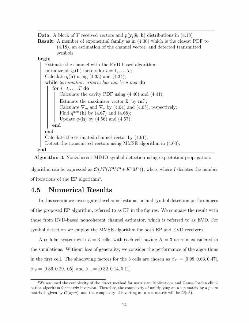
Data: A block of T received vectors and p(yt|st,h) distributions in (4.18)Result: A member of exponential family as in (4.30) which is the closest PDF to
(4.18), an estimation of the channel vector, and detected transmittedsymbols
begin
Estimate the channel with the EVD-based algorithm;Initialize all qt(h) factors for t = 1, . . . , T ;Calculate q(h) using (4.33) and (4.34);while termination criteria has not been met do
for t=1,. . . ,T do
Calculate the cavity PDF using (4.40) and (4.41);
Estimate the maximizer vector xt by m\th ;
Calculate ∇m and ∇v by (4.64) and (4.65), respectively;Find qnew(h) by (4.67) and (4.68);Update qt(h) by (4.56) and (4.57);
end
end
Calculate the estimated channel vector by (4.61);Detect the transmitted vectors using MMSE algorithm in (4.63);
end
Algorithm 3: Noncoherent MIMO symbol detection using expectation propagation.
algorithm can be expressed as O(
IT (K3M3+K2M2))
, where where I denotes the number
of iterations of the EP algorithm4.
4.5 Numerical Results
In this section we investigate the channel estimation and symbol detection performances
of the proposed EP algorithm, referred to as EP in the figures. We compare the result with
those from EVD-based noncoherent channel estimator, which is referred to as EVD. For
symbol detection we employ the MMSE algorithm for both EP and EVD receivers.
A cellular system with L = 3 cells, with each cell having K = 3 users is considered in
the simulations. Without loss of generality, we consider the performance of the algorithms
in the first cell. The shadowing factors for the 3 cells are chosen as β11 = [0.98, 0.63, 0.47],
β12 = [0.36, 0.29, .05], and β13 = [0.32, 0.14, 0.11].
4We assumed the complexity of the direct method for matrix multiplications and Gauss-Jordan elimi-nation algorithm for matrix inversion. Therefore, the complexity of multiplying an n×p matrix by a p×mmatrix is given by O(npm), and the complexity of inverting an n× n matrix will be O(n3).
74
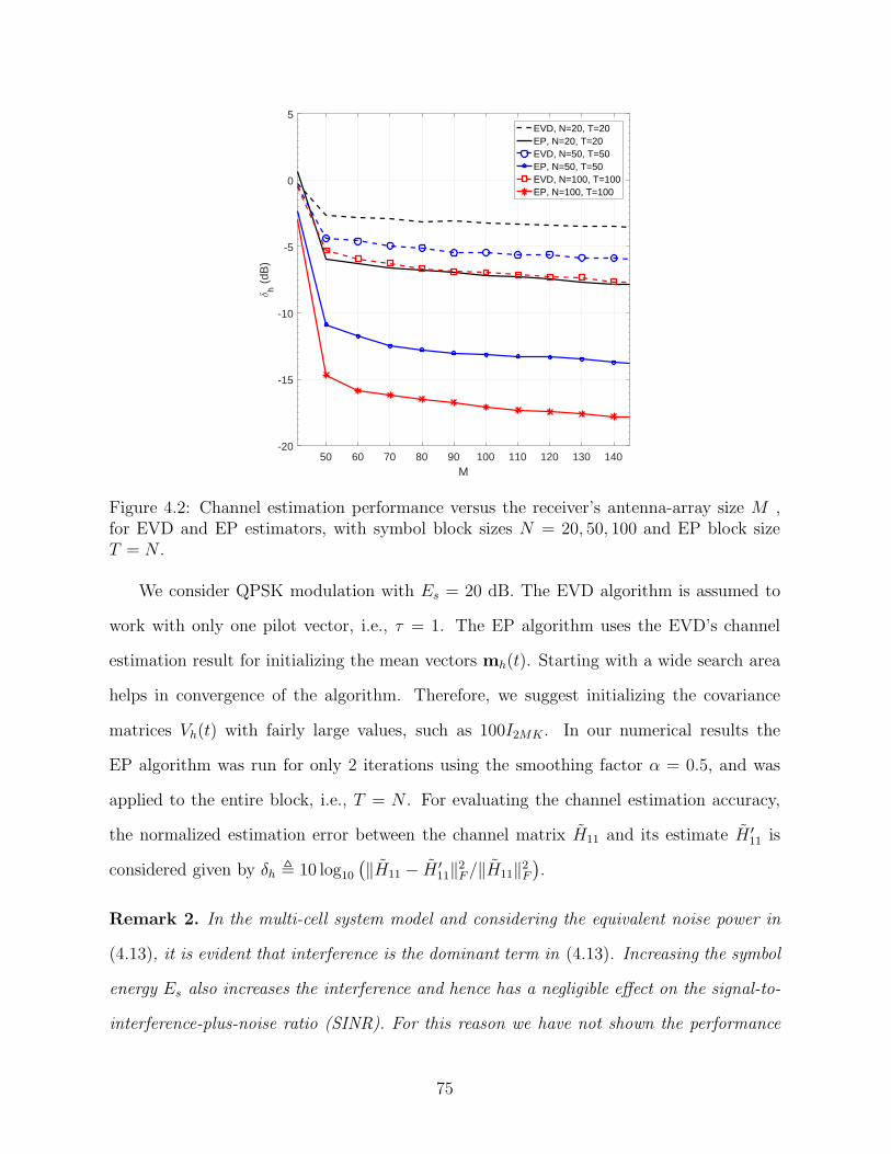
50 60 70 80 90 100 110 120 130 140M
-20
-15
-10
-5
0
5
δh (
dB)
EVD, N=20, T=20EP, N=20, T=20EVD, N=50, T=50EP, N=50, T=50EVD, N=100, T=100EP, N=100, T=100
Figure 4.2: Channel estimation performance versus the receiver’s antenna-array size M ,for EVD and EP estimators, with symbol block sizes N = 20, 50, 100 and EP block sizeT = N .
We consider QPSK modulation with Es = 20 dB. The EVD algorithm is assumed to
work with only one pilot vector, i.e., τ = 1. The EP algorithm uses the EVD’s channel
estimation result for initializing the mean vectors mh(t). Starting with a wide search area
helps in convergence of the algorithm. Therefore, we suggest initializing the covariance
matrices Vh(t) with fairly large values, such as 100I2MK . In our numerical results the
EP algorithm was run for only 2 iterations using the smoothing factor α = 0.5, and was
applied to the entire block, i.e., T = N . For evaluating the channel estimation accuracy,
the normalized estimation error between the channel matrix H11 and its estimate H ′11 is
considered given by δh , 10 log10(
‖H11 − H ′11‖2F/‖H11‖2F
)
.
Remark 2. In the multi-cell system model and considering the equivalent noise power in
(4.13), it is evident that interference is the dominant term in (4.13). Increasing the symbol
energy Es also increases the interference and hence has a negligible effect on the signal-to-
interference-plus-noise ratio (SINR). For this reason we have not shown the performance
75
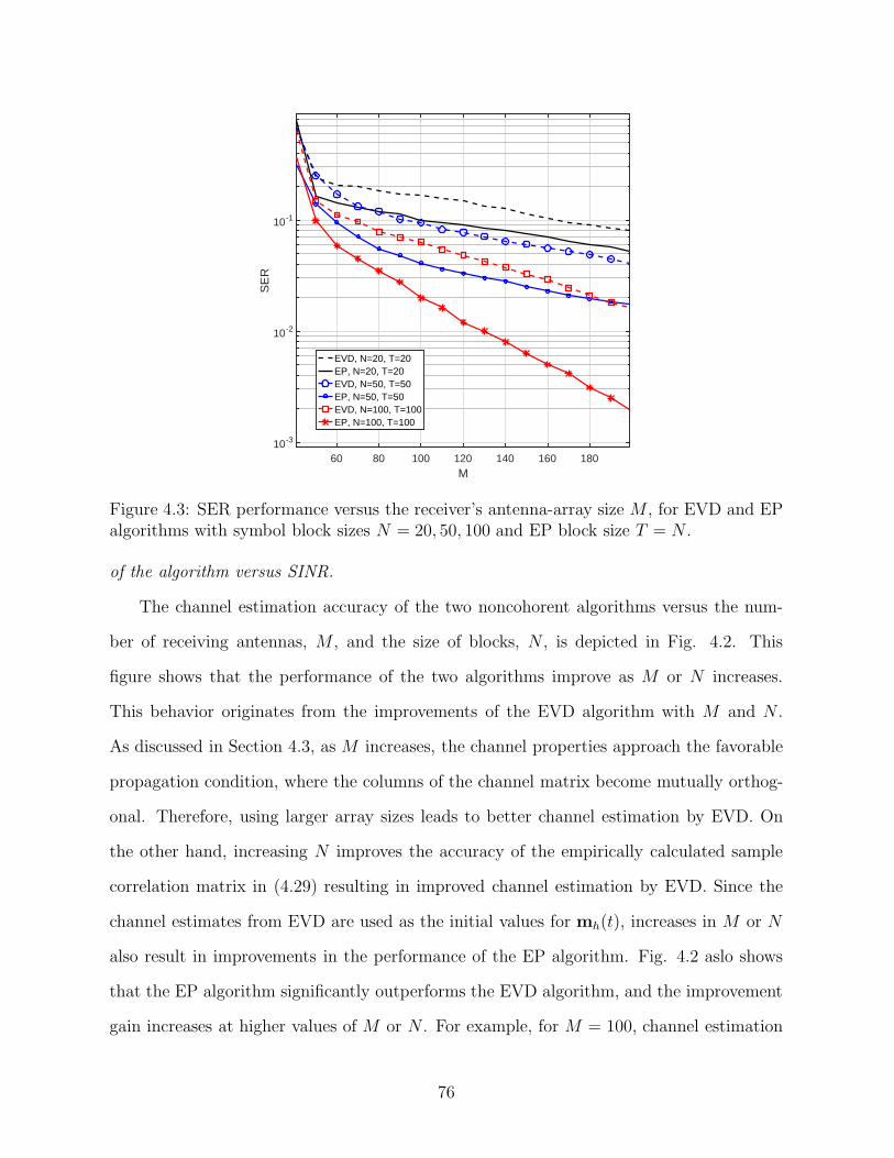
60 80 100 120 140 160 180M
10-3
10-2
10-1
SE
R
EVD, N=20, T=20EP, N=20, T=20EVD, N=50, T=50EP, N=50, T=50EVD, N=100, T=100EP, N=100, T=100
Figure 4.3: SER performance versus the receiver’s antenna-array size M , for EVD and EPalgorithms with symbol block sizes N = 20, 50, 100 and EP block size T = N .
of the algorithm versus SINR.
The channel estimation accuracy of the two noncohorent algorithms versus the num-
ber of receiving antennas, M , and the size of blocks, N , is depicted in Fig. 4.2. This
figure shows that the performance of the two algorithms improve as M or N increases.
This behavior originates from the improvements of the EVD algorithm with M and N .
As discussed in Section 4.3, as M increases, the channel properties approach the favorable
propagation condition, where the columns of the channel matrix become mutually orthog-
onal. Therefore, using larger array sizes leads to better channel estimation by EVD. On
the other hand, increasing N improves the accuracy of the empirically calculated sample
correlation matrix in (4.29) resulting in improved channel estimation by EVD. Since the
channel estimates from EVD are used as the initial values for mh(t), increases in M or N
also result in improvements in the performance of the EP algorithm. Fig. 4.2 aslo shows
that the EP algorithm significantly outperforms the EVD algorithm, and the improvement
gain increases at higher values of M or N . For example, for M = 100, channel estimation
76
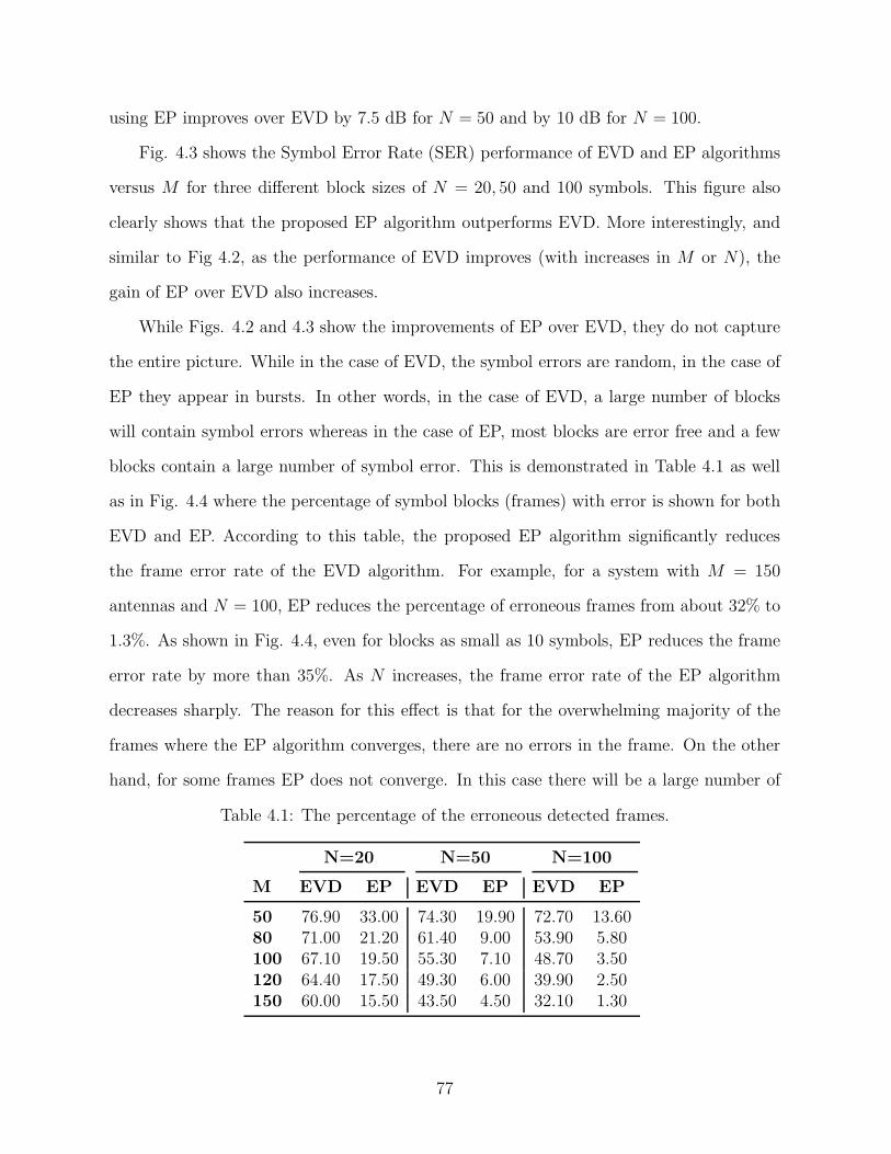
using EP improves over EVD by 7.5 dB for N = 50 and by 10 dB for N = 100.
Fig. 4.3 shows the Symbol Error Rate (SER) performance of EVD and EP algorithms
versus M for three different block sizes of N = 20, 50 and 100 symbols. This figure also
clearly shows that the proposed EP algorithm outperforms EVD. More interestingly, and
similar to Fig 4.2, as the performance of EVD improves (with increases in M or N), the
gain of EP over EVD also increases.
While Figs. 4.2 and 4.3 show the improvements of EP over EVD, they do not capture
the entire picture. While in the case of EVD, the symbol errors are random, in the case of
EP they appear in bursts. In other words, in the case of EVD, a large number of blocks
will contain symbol errors whereas in the case of EP, most blocks are error free and a few
blocks contain a large number of symbol error. This is demonstrated in Table 4.1 as well
as in Fig. 4.4 where the percentage of symbol blocks (frames) with error is shown for both
EVD and EP. According to this table, the proposed EP algorithm significantly reduces
the frame error rate of the EVD algorithm. For example, for a system with M = 150
antennas and N = 100, EP reduces the percentage of erroneous frames from about 32% to
1.3%. As shown in Fig. 4.4, even for blocks as small as 10 symbols, EP reduces the frame
error rate by more than 35%. As N increases, the frame error rate of the EP algorithm
decreases sharply. The reason for this effect is that for the overwhelming majority of the
frames where the EP algorithm converges, there are no errors in the frame. On the other
hand, for some frames EP does not converge. In this case there will be a large number of
Table 4.1: The percentage of the erroneous detected frames.
N=20 N=50 N=100
M EVD EP EVD EP EVD EP
50 76.90 33.00 74.30 19.90 72.70 13.6080 71.00 21.20 61.40 9.00 53.90 5.80100 67.10 19.50 55.30 7.10 48.70 3.50120 64.40 17.50 49.30 6.00 39.90 2.50150 60.00 15.50 43.50 4.50 32.10 1.30
77
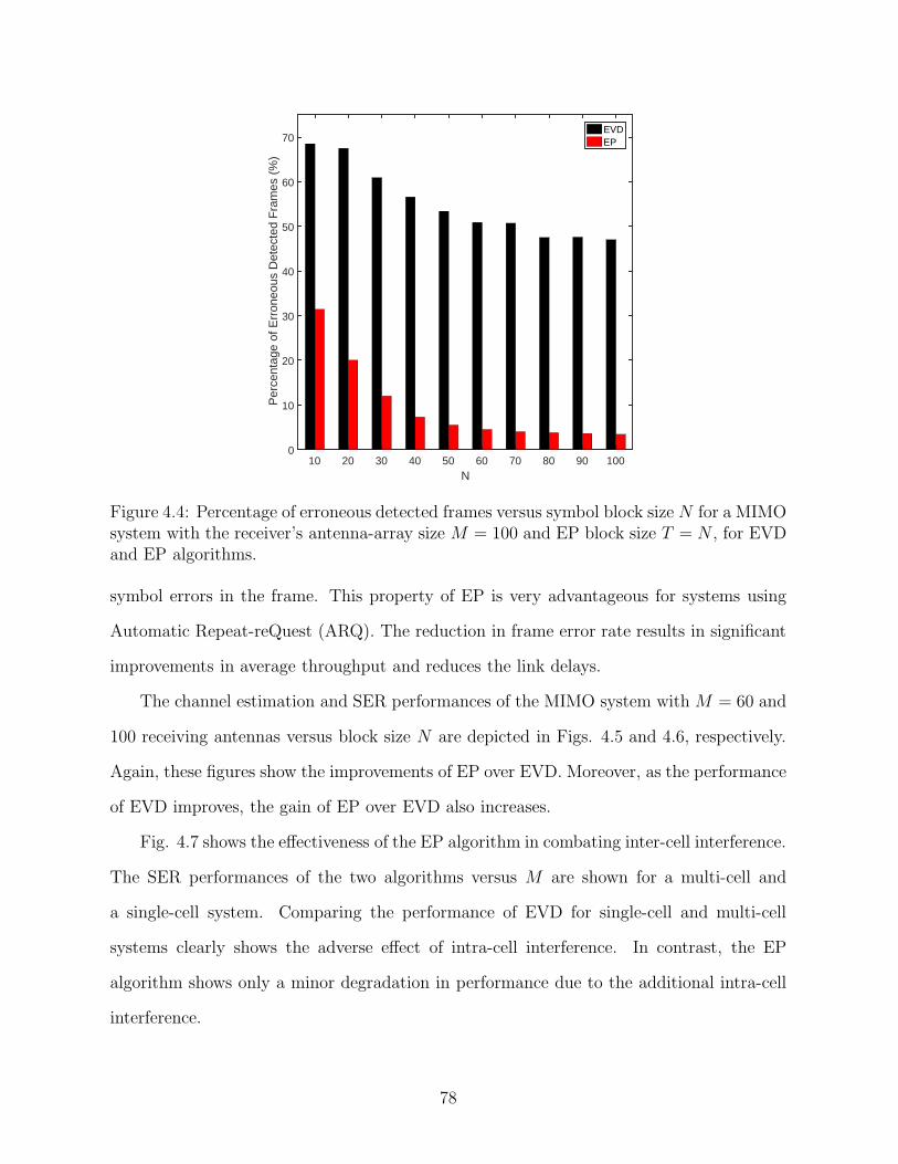
10 20 30 40 50 60 70 80 90 100N
0
10
20
30
40
50
60
70
Per
cent
age
of E
rron
eous
Det
ecte
d F
ram
es (
%)
EVDEP
Figure 4.4: Percentage of erroneous detected frames versus symbol block size N for a MIMOsystem with the receiver’s antenna-array size M = 100 and EP block size T = N , for EVDand EP algorithms.
symbol errors in the frame. This property of EP is very advantageous for systems using
Automatic Repeat-reQuest (ARQ). The reduction in frame error rate results in significant
improvements in average throughput and reduces the link delays.
The channel estimation and SER performances of the MIMO system with M = 60 and
100 receiving antennas versus block size N are depicted in Figs. 4.5 and 4.6, respectively.
Again, these figures show the improvements of EP over EVD. Moreover, as the performance
of EVD improves, the gain of EP over EVD also increases.
Fig. 4.7 shows the effectiveness of the EP algorithm in combating inter-cell interference.
The SER performances of the two algorithms versus M are shown for a multi-cell and
a single-cell system. Comparing the performance of EVD for single-cell and multi-cell
systems clearly shows the adverse effect of intra-cell interference. In contrast, the EP
algorithm shows only a minor degradation in performance due to the additional intra-cell
interference.
78
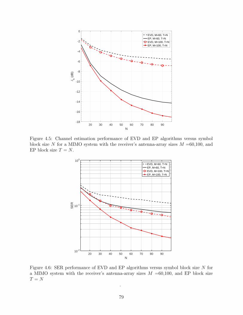
20 30 40 50 60 70 80 90N
-18
-16
-14
-12
-10
-8
-6
-4
-2
0
δh (
dB)
EVD, M=60, T=NEP, M=60, T=NEVD, M=100, T=NEP, M=100, T=N
Figure 4.5: Channel estimation performance of EVD and EP algorithms versus symbolblock size N for a MIMO system with the receiver’s antenna-array sizes M =60,100, andEP block size T = N .
20 30 40 50 60 70 80 90N
10-2
10-1
100
SE
R
EVD, M=60, T=NEP, M=60, T=NEVD, M=100, T=NEP, M=100, T=N
Figure 4.6: SER performance of EVD and EP algorithms versus symbol block size N fora MIMO system with the receiver’s antenna-array sizes M =60,100, and EP block sizeT = N
.
79
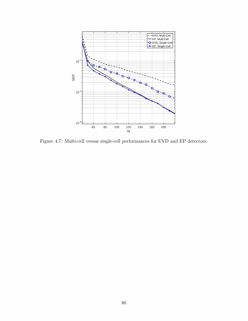
60 80 100 120 140 160 180M
10-3
10-2
10-1
SE
R
EVD, Multi-CellEP, Multi-CellEVD, Single-CellEP, Single-Cell
Figure 4.7: Multi-cell versus single-cell performances for EVD and EP detectors.
80
Chapter 5
Conclusion
In Chapter 2 we investigate the performance of the expectation propagation (EP) detec-
tor in practical situations in which perfect channel state information (CSI) is not available
at the receiver. As expected and verified by the simulation results, lack of perfect CSI re-
sults in significant performance loss for the EP detector. Moreover, the EP detector shows
a higher sensitivity to the channel estimation error at high signal-to-noise ratios (SNR) and
the rate of its performance improvement decreases at higher SNRs. To rectify this problem
we propose a Modified EP algorithm for correlated noise which utilizes the correlation ma-
trix of the channel estimation error. Simulation results show that the modified algorithm
is robust against imperfect CSI and its performance is significantly improved over the EP
algorithm.
A noncoherent detector for large-scale SIMO systems using the Expectation Propaga-
tion algorithm is proposed in Chapter 3. We show through simulation that with only a
single iteration and for block sizes as small as two symbols, the proposed algorithm outper-
forms the pilot-based MMSE detector in term of symbol error rate (SER). This property
makes the proposed algorithm suitable for channels with coherence times as short as two
symbol durations. Moreover, the simulation results verify that as the symbol block size
increases, the SER performance of the algorithm converges to that of the optimal ML re-
ceiver which has perfect knowledge of channel state information. The proposed detector
does not rely on prior knowledge of channel statistics and it is shown that for a Rician
fading channel, it can outperform the coherent MMSE detector without using Rician K-
factor. Finally, the proposed method does not rely on specific signal constellations and can
be used for any differential modulation scheme.
In Chapter 4 we propose a noncoherent channel estimation and symbol detection al-
gorithm for multi-cell multi-user massive MIMO systems based on the expectation propa-
81
gation algorithm. The proposed algorithm is initialized with the channel estimation result
from the EVD-based method. Simulation results show that after a few iterations, the
EP-based algorithm significantly outperforms the EVD-based method in both channel es-
timation and symbol error rate. Moreover, the EP-based algorithm is not sensitive to
antenna array size or the inaccuracies of sample correlation matrix.
82
References[1] J. Vieira, S. Malkowsky, K. Nieman, Z. Miers, N. Kundargi, L. Liu, I. Wong, V. wall,
O. Edfors, and F. Tufvesson, “A flexible 100-antenna testbed for massive MIMO,” in2014 IEEE Globecom Workshops (GC Wkshps), Dec 2014, pp. 287–293.
[2] the network, cisco’s technology news site. [Online]. Available:https://newsroom.cisco.com/press-release-content?articleId=1741352# ftn1.
[3] cisco. [Online]. Available: http://www.cisco.com/c/en/us/solutions/service-provider/visual-networking-index-vni/index.html.
[4] G. J. Foschini, “Layered space-time architecture for wireless communication in a fadingenvironment when using multi-element antennas,” Bell Labs Technical Journal, vol. 1,no. 2, pp. 41–59, Autumn 1996.
[5] E. Telatar, “Capacity of multi-antenna gaussian channels.” European Transactionson Telecommunications, vol. 10, no. 6, pp. 585–595, 1999. [Online]. Available:http://dblp.uni-trier.de/db/journals/ett/ett10.html#Telatar99
[6] G. J. Foschini and M. J. Gans, “On limits of wireless communications in a fadingenvironment when using multiple antennas.” Wireless Personal Communications,vol. 6, no. 3, pp. 311–335, 1998. [Online]. Available: http://dblp.uni-trier.de/db/journals/wpc/wpc6.html#FoschiniG98
[7] J. Hampton, Introduction to MIMO communications. Cambridge: Cambridge Uni-versity Press, 2014.
[8] T. Marzetta, “Noncooperative cellular wireless with unlimited numbers of base stationantennas,” Wireless Communications, IEEE Transactions on, vol. 9, no. 11, pp. 3590–3600, November 2010.
[9] F. Rusek, D. Persson, B. K. Lau, E. G. Larsson, T. L. Marzetta, O. Edfors, andF. Tufvesson, “Scaling up MIMO: Opportunities and challenges with very large ar-rays,” IEEE Signal Processing Magazine, vol. 30, no. 1, pp. 40–60, Jan 2013.
[10] L. Lu, G. Li, A. Swindlehurst, A. Ashikhmin, and R. Zhang, “An overview of massiveMIMO: Benefits and challenges,” Selected Topics in Signal Processing, IEEE Journalof, vol. 8, no. 5, pp. 742–758, Oct 2014.
[11] E. Bjornson, E. G. Larsson, and T. L. Marzetta, “Massive MIMO: ten myths andone critical question,” IEEE Communications Magazine, vol. 54, no. 2, pp. 114–123,February 2016.
[12] B. Hochwald, T. Marzetta, and V. Tarokh, “Multiple-antenna channel hardening andits implications for rate feedback and scheduling,” Information Theory, IEEE Trans-actions on, vol. 50, no. 9, pp. 1893–1909, Sept 2004.
[13] C. Zhang and R. Qiu, “Massive MIMO as a big data system: Random matrix modelsand testbed,” Access, IEEE, vol. 3, pp. 837–851, 2015.
83
[14] J. Vieira, S. Malkowsky, K. Nieman, Z. Miers, N. Kundargi, L. Liu, I. Wong, V. Owall,O. Edfors, and F. Tufvesson, “A flexible 100-antenna testbed for massive MIMO,” inGlobecom Workshops (GC Wkshps), 2014, Dec 2014, pp. 287–293.
[15] P. Harris, S. Zang, A. Nix, M. Beach, S. Armour, and A. Doufexi, “A distributedmassive MIMO testbed to assess real-world performance and feasibility,” in VehicularTechnology Conference (VTC Spring), 2015 IEEE 81st, May 2015, pp. 1–2.
[16] A. Tulino and S. Verdu, Random matrix theory and wireless communications. Delft,The Netherlands: Now Publishers, Inc., 2004.
[17] A. Chockalingam and B. Rajan, Large MIMO Systems, ser. Large MIMO Systems.Cambridge University Press, 2014.
[18] S. Vishwanath, N. Jindal, and A. Goldsmith, “Duality, achievable rates, and sum-ratecapacity of gaussian MIMO broadcast channels,” IEEE Transactions on InformationTheory, vol. 49, no. 10, pp. 2658–2668, Oct 2003.
[19] H. Q. Ngo, E. G. Larsson, and T. L. Marzetta, “Energy and spectral efficiency of verylarge multiuser MIMO systems,” IEEE Transactions on Communications, vol. 61,no. 4, pp. 1436–1449, April 2013.
[20] C. Kong, C. Zhong, A. K. Papazafeiropoulos, M. Matthaiou, and Z. Zhang, “Effectof channel aging on the sum rate of uplink massive MIMO systems,” in 2015 IEEEInternational Symposium on Information Theory (ISIT), June 2015, pp. 1222–1226.
[21] G. Amarasuriya and H. Poor, “Impact of channel aging in multi-way relay networkswith massive MIMO,” in Communications (ICC), 2015 IEEE International Conferenceon, June 2015, pp. 1951–1957.
[22] K. Truong and R. Heath, “Effects of channel aging in massive MIMO systems,” Com-munications and Networks, Journal of, vol. 15, no. 4, pp. 338–351, Aug 2013.
[23] T. Weber, A. Sklavos, and M. Meurer, “Imperfect channel-state information in MIMOtransmission,” Communications, IEEE Transactions on, vol. 54, no. 3, pp. 543–552,March 2006.
[24] J. Proakis and M. Salehi, Digital Communications. New York: McGraw-Hill, 2008.
[25] G. J. Foschini, “Layered space-time architecture for wireless communication in a fadingenvironment when using multi-element antennas,” Bell labs technical journal, vol. 1,no. 2, pp. 41–59, 1996.
[26] G. Ginis and J. Cioffi, “On the relation between v-blast and the gdfe,” CommunicationsLetters, IEEE, vol. 5, no. 9, pp. 364–366, Sept 2001.
[27] J. Hoydis, S. ten Brink, and M. Debbah, “Massive MIMO in the ul/dl of cellularnetworks: How many antennas do we need?” IEEE Journal on Selected Areas inCommunications, vol. 31, no. 2, pp. 160–171, February 2013.
84
[28] F. Kschischang, B. Frey, and H.-A. Loeliger, “Factor graphs and the sum-productalgorithm,” Information Theory, IEEE Transactions on, vol. 47, no. 2, pp. 498–519,Feb 2001.
[29] J. Goldberger and A. Leshem, “MIMO detection for high-order qam based on a gaus-sian tree approximation,” IEEE Transactions on Information Theory, vol. 57, no. 8,pp. 4973–4982, Aug 2011.
[30] J. Goldberger, “Improved MIMO detection based on successive tree approximations,”in Information Theory Proceedings (ISIT), 2013 IEEE International Symposium on,July 2013, pp. 2004–2008.
[31] T. P. Minka, “Expectation propagation for approximate bayesian inference,” in Pro-ceedings of the Seventeenth conference on Uncertainty in artificial intelligence. Mor-gan Kaufmann Publishers Inc., 2001, pp. 362–369.
[32] J. Cespedes, P. M. Olmos, M. Sanchez-Fernandez, and F. Perez-Cruz, “Expectationpropagation detection for high-order high-dimensional MIMO systems,” IEEE Trans-actions on Communications, vol. 62, no. 8, pp. 2840–2849, Aug 2014.
[33] H. Zhang, S. Gao, D. Li, H. Chen, and L. Yang, “On superimposed pilot for channelestimation in multi-cell multiuser MIMO uplink: Large system analysis,” VehicularTechnology, IEEE Transactions on, vol. PP, no. 99, pp. 1–1, 2015.
[34] T. Bogale and L. B. Le, “Pilot optimization and channel estimation for multiusermassive MIMO systems,” in Information Sciences and Systems (CISS), 2014 48thAnnual Conference on, March 2014, pp. 1–6.
[35] C.-K. Wen, S. Jin, K.-K. Wong, J.-C. Chen, and P. Ting, “Channel estimation formassive MIMO using gaussian-mixture bayesian learning,” Wireless Communications,IEEE Transactions on, vol. 14, no. 3, pp. 1356–1368, March 2015.
[36] A. K. Papazafeiropoulos and T. Ratnarajah, “Deterministic equivalent performanceanalysis of time-varying massive MIMO systems,” IEEE Transactions on WirelessCommunications, vol. 14, no. 10, pp. 5795–5809, Oct 2015.
[37] B. S. Thian and A. Goldsmith, “Decoding for MIMO systems with imperfect channelstate information,” in Global Telecommunications Conference (GLOBECOM 2010),2010 IEEE, Dec 2010, pp. 1–6.
[38] T. Minka, “A family of algorithms for approximate Bayesianinference,” PhD thesis, MIT, 2001. [Online]. Available:http://research.microsoft.com/ minka/papers/ep/minka-thesis.pdf
[39] S. M. Kay, Fundamentals of Statistical Signal Processing: Estimation Theory. PrenticeHall, 1997.
[40] M. Seeger, “Expectation propagation for exponential families,” University of Califor-nia, Berkeley, CA, USA, Tech. Rep., 2005.
85
[41] J. P. Kermoal, L. Schumacher, K. I. Pedersen, P. E. Mogensen, and F. Frederiksen, “Astochastic MIMO radio channel model with experimental validation,” IEEE Journalon Selected Areas in Communications, vol. 20, no. 6, pp. 1211–1226, Aug 2002.
[42] B. Hassibi and B. Hochwald, “How much training is needed in multiple-antenna wire-less links?” Information Theory, IEEE Transactions on, vol. 49, no. 4, pp. 951–963,April 2003.
[43] R. Gold, “Optimal binary sequences for spread spectrum multiplexing (corresp.),”IEEE Transactions on Information Theory, vol. 13, no. 4, pp. 619–621, October 1967.
[44] T. L. Marzetta, “How much training is required for multiuser mimo?” in 2006 FortiethAsilomar Conference on Signals, Systems and Computers, Oct 2006, pp. 359–363.
[45] M. Stojnic and B. Hassibi, “Out-sphere decoder for non-coherent ml SIMO detectionand its expected complexity,” in 2007 Conference Record of the Forty-First AsilomarConference on Signals, Systems and Computers, Nov 2007, pp. 1568–1572.
[46] H. A. J. Alshamary, T. Al-Naffouri, A. Zaib, and W. Xu, “Optimal non-coherent datadetection for massive SIMO wireless systems: A polynomial complexity solution,” inSignal Processing and Signal Processing Education Workshop (SP/SPE), 2015 IEEE,Aug 2015, pp. 172–177.
[47] M. Chowdhury, A. Manolakos, and A. J. Goldsmith, “Design and performance ofnoncoherent massive simo systems,” in Information Sciences and Systems (CISS),2014 48th Annual Conference on, March 2014, pp. 1–6.
[48] B. Knott, M. Chowdhury, A. Manolakos, and A. J. Goldsmith, “Benefits of codingin a noncoherent massive SIMO system,” in 2015 IEEE International Conference onCommunications (ICC), June 2015, pp. 2350–2355.
[49] A. Manolakos, M. Chowdhury, and A. J. Goldsmith, “Constellation design in non-coherent massive SIMO systems,” in 2014 IEEE Global Communications Conference,Dec 2014, pp. 3690–3695.
[50] A. G. Armada and L. Hanzo, “A non-coherent multi-user large scale SIMO systemrelaying on m-ary dpsk,” in 2015 IEEE International Conference on Communications(ICC), June 2015, pp. 2517–2522.
[51] Y. Qi and T. P. Minka, “Window-based expectation propagation for adaptive signaldetection in flat-fading channels,” IEEE Transactions on Wireless Communications,vol. 6, no. 1, pp. 348–355, Jan 2007.
[52] O. Elijah, C. Y. Leow, T. A. Rahman, S. Nunoo, and S. Z. Iliya, “A comprehensivesurvey of pilot contamination in massive MIMO-5G system,” IEEE CommunicationsSurveys Tutorials, vol. 18, no. 2, pp. 905–923, Secondquarter 2016.
[53] K. Ghavami and M. Naraghi-Pour, “Noncoherent SIMO detection by expectation prop-agation,” in 2017 IEEE International Conference on Communications (ICC), 2017.
86
[54] H. Q. Ngo and E. G. Larsson, “Evd-based channel estimation in multicell multiuserMIMO systems with very large antenna arrays,” in 2012 IEEE International Confer-ence on Acoustics, Speech and Signal Processing (ICASSP), March 2012, pp. 3249–3252.
[55] L. Cottatellucci, R. R. Muller, and M. Vehkapera, “Analysis of pilot decontaminationbased on power control,” in 2013 IEEE 77th Vehicular Technology Conference (VTCSpring), June 2013, pp. 1–5.
[56] R. R. Muller, L. Cottatellucci, and M. Vehkapera, “Blind pilot decontamination,”IEEE Journal of Selected Topics in Signal Processing, vol. 8, no. 5, pp. 773–786, Oct2014.
[57] R. R. Muller, M. Vehkapera, and L. Cottatellucci, “Analysis of blind pilot decontami-nation,” in 2013 Asilomar Conference on Signals, Systems and Computers, Nov 2013,pp. 1016–1020.
[58] J. Vinogradova, E. Bjornson, and E. G. Larsson, “On the separability of signal andinterference-plus-noise subspaces in blind pilot decontamination,” in 2016 IEEE In-ternational Conference on Acoustics, Speech and Signal Processing (ICASSP), March2016, pp. 3421–3425.
[59] C. K. Wen, S. Jin, K. K. Wong, J. C. Chen, and P. Ting, “Channel estimation for mas-sive MIMO using gaussian-mixture bayesian learning,” IEEE Transactions on WirelessCommunications, vol. 14, no. 3, pp. 1356–1368, March 2015.
[60] K. Ghavami and M. Naraghi-Pour, “MIMO detection with imperfect channel stateinformation using expectation propagation,” IEEE Transactions on Vehicular Tech-nology, vol. PP, no. 99, pp. 1–1, 2017.
[61] J. Yedidia, W. Freeman, and Y. Weiss, “Understanding belief propagation andits generalizations,” in Exploring Artificial Intelligence in the New Millennium,G. Lakemeyer and B. Nebel, Eds. Morgan Kaufmann Publishers, Jan. 2003, ch. 8,pp. 239–236. [Online]. Available: http://www.merl.com/publications/TR2001-22
[62] F. R. Kschischang, B. J. Frey, and H. A. Loeliger, “Factor graphs and the sum-productalgorithm,” IEEE Transactions on Information Theory, vol. 47, no. 2, pp. 498–519,Feb 2001.
[63] J. S. Yedidia, W. T. Freeman, and Y. Weiss, “Constructing free-energy approximationsand generalized belief propagation algorithms,” IEEE Transactions on InformationTheory, vol. 51, no. 7, pp. 2282–2312, July 2005.
[64] J. Hu and T. M. Duman, “Graph-based detector for blast architecture,” in 2007 IEEEInternational Conference on Communications, June 2007, pp. 1018–1023.
87
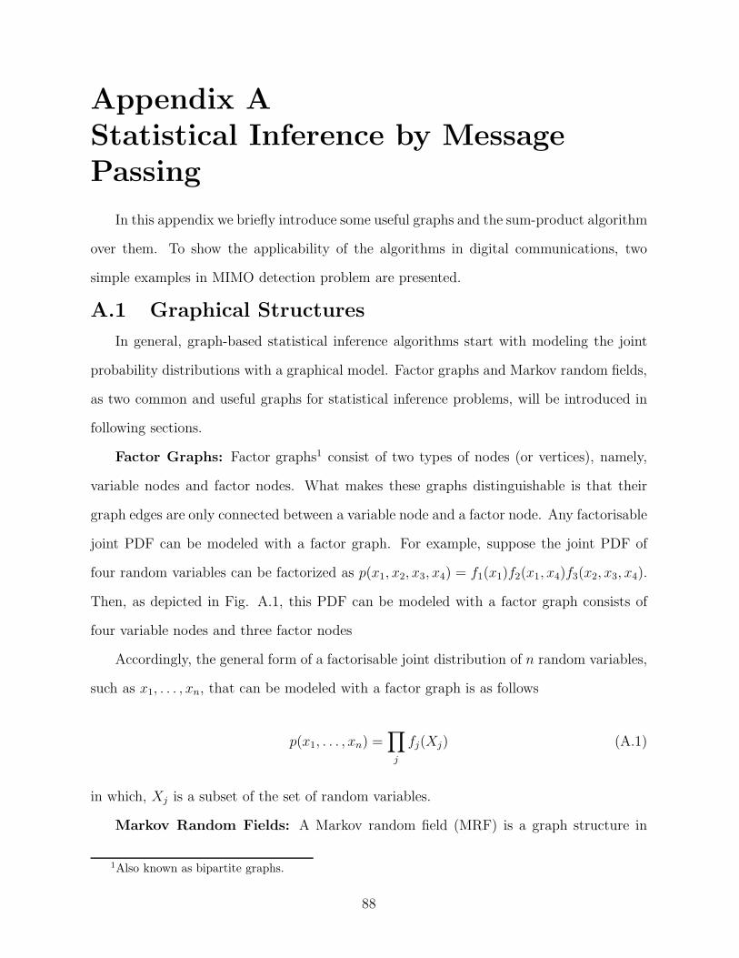
Appendix A
Statistical Inference by Message
Passing
In this appendix we briefly introduce some useful graphs and the sum-product algorithm
over them. To show the applicability of the algorithms in digital communications, two
simple examples in MIMO detection problem are presented.
A.1 Graphical Structures
In general, graph-based statistical inference algorithms start with modeling the joint
probability distributions with a graphical model. Factor graphs and Markov random fields,
as two common and useful graphs for statistical inference problems, will be introduced in
following sections.
Factor Graphs: Factor graphs1 consist of two types of nodes (or vertices), namely,
variable nodes and factor nodes. What makes these graphs distinguishable is that their
graph edges are only connected between a variable node and a factor node. Any factorisable
joint PDF can be modeled with a factor graph. For example, suppose the joint PDF of
four random variables can be factorized as p(x1, x2, x3, x4) = f1(x1)f2(x1, x4)f3(x2, x3, x4).
Then, as depicted in Fig. A.1, this PDF can be modeled with a factor graph consists of
four variable nodes and three factor nodes
Accordingly, the general form of a factorisable joint distribution of n random variables,
such as x1, . . . , xn, that can be modeled with a factor graph is as follows
p(x1, . . . , xn) =∏
j
fj(Xj) (A.1)
in which, Xj is a subset of the set of random variables.
Markov Random Fields: A Markov random field (MRF) is a graph structure in
1Also known as bipartite graphs.
88
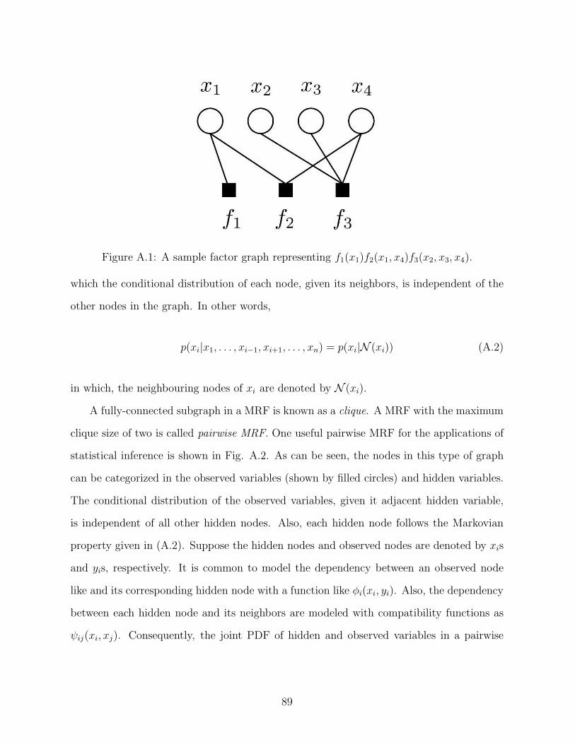
Figure A.1: A sample factor graph representing f1(x1)f2(x1, x4)f3(x2, x3, x4).
which the conditional distribution of each node, given its neighbors, is independent of the
other nodes in the graph. In other words,
p(xi|x1, . . . , xi−1, xi+1, . . . , xn) = p(xi|N (xi)) (A.2)
in which, the neighbouring nodes of xi are denoted by N (xi).
A fully-connected subgraph in a MRF is known as a clique. A MRF with the maximum
clique size of two is called pairwise MRF. One useful pairwise MRF for the applications of
statistical inference is shown in Fig. A.2. As can be seen, the nodes in this type of graph
can be categorized in the observed variables (shown by filled circles) and hidden variables.
The conditional distribution of the observed variables, given it adjacent hidden variable,
is independent of all other hidden nodes. Also, each hidden node follows the Markovian
property given in (A.2). Suppose the hidden nodes and observed nodes are denoted by xis
and yis, respectively. It is common to model the dependency between an observed node
like and its corresponding hidden node with a function like φi(xi, yi). Also, the dependency
between each hidden node and its neighbors are modeled with compatibility functions as
ψij(xi, xj). Consequently, the joint PDF of hidden and observed variables in a pairwise
89
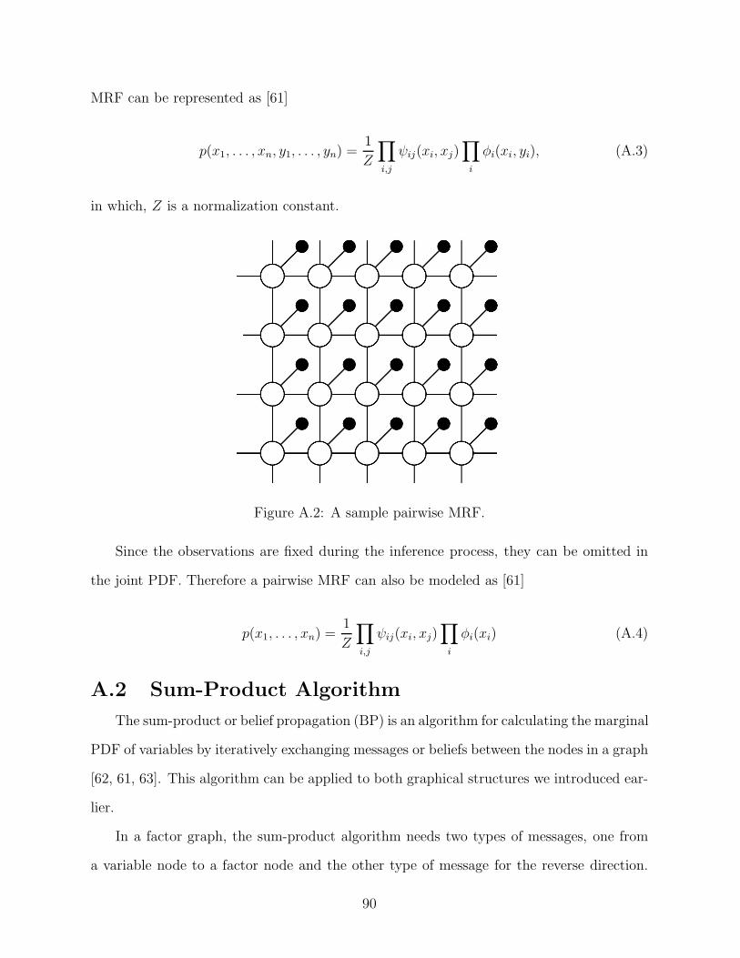
MRF can be represented as [61]
p(x1, . . . , xn, y1, . . . , yn) =1
Z
∏
i,j
ψij(xi, xj)∏
i
φi(xi, yi), (A.3)
in which, Z is a normalization constant.
Figure A.2: A sample pairwise MRF.
Since the observations are fixed during the inference process, they can be omitted in
the joint PDF. Therefore a pairwise MRF can also be modeled as [61]
p(x1, . . . , xn) =1
Z
∏
i,j
ψij(xi, xj)∏
i
φi(xi) (A.4)
A.2 Sum-Product Algorithm
The sum-product or belief propagation (BP) is an algorithm for calculating the marginal
PDF of variables by iteratively exchanging messages or beliefs between the nodes in a graph
[62, 61, 63]. This algorithm can be applied to both graphical structures we introduced ear-
lier.
In a factor graph, the sum-product algorithm needs two types of messages, one from
a variable node to a factor node and the other type of message for the reverse direction.
90
Following the well-known notation in [62], the sum-product messages from a variable node
x to a factor node f , and vice versa, in a factor graph are given as follows
µx→f(x) =∏
h∈N (x)\{f}
µh→x(x) (A.5)
and
µf→x(x) =∑
∼{x}
f(X)∏
y∈N (f)\{x}
µy→f(y) (A.6)
where, N (x) shows the neighbours of x, ∼ {x} means all variables but x, and the backslash
signes in \{f} and \{x} simply mean excluding the factor node f or variable node x,
respectively. After algorithm’s convergence, the marginal distribution of each variable
node can be calculated as
f(x) =∏
h∈N (x)
µh→x(x) (A.7)
The sum-product algorith can be implemented in pairwise MRF by exchanging the
following message between the hidden nodes[61]:
mij(xj) =∑
xi
φi(xi)ψij(xi, xj)∏
k∈N (i)\j
mki(xi). (A.8)
which can also be considered as the believe of the i-th hidden node in the value of the j-th
hidden node. Finally, the belief of the i-th hidden node is given as
bi(xi) = kφi(xi)∏
j∈N (i)
mji(xi). (A.9)
91
A.3 Applications of the BP Algorithm in MIMO De-
tection
To show the applicability of the BP algorithm to digital communications, in this section
we present two examples of MIMO detection by this algorithm.
Assume a MIMO system with M receiving and K transmitting antennas. The received
vector for this model is given as
y = Hx+ n, (A.10)
in which, y ∈ CM×1 is the received vector, x ∈ CK×1 is the vector of K transmitted symbols
as x = [x1, . . . , xK ]T , n ∈ CM×1 is the AWGN noise vector with distribution CN (0, σ2IM),
and H ∈ CM×K is the known channel matrix.
MIMO detection can be considered as a statistical inference problem. In fact, the sym-
bol detection is equivalent to find the marginal PDF of the transmitted vectors. Therefore,
as we will show in following parts, by assigning the transmitted symbols to the variable
nodes of a factor graph or the hidden nodes of a pairwise MRF, it is possible to iteratively
find their marginals by BP algorithm.
MIMO Detection by Factor Graph Model: As is depicted in Fig.A.3, the MIMO
detection problem can be modeled with a factor graph where its variable nodes are the
transmitted symbols and its factor nodes are the received signals [64]. This leads to a
densely connected graph with lots of cycles which affect the detection performance and
accuracy of the detector.
By assuming BPSK symbols, the log likelihood ratio of the j-th transmitted symbol
given the i-th received signal is given as
logp(xj = 0|yi)p(xj = 1|yi)
= log
∑
x,xj=0 p(x|yi)∑
x,xj=1 p(x|yi)
92
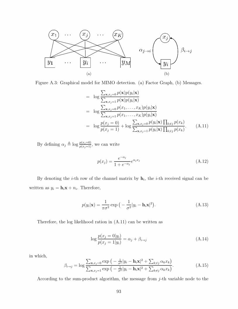
(a) (b)
Figure A.3: Graphical model for MIMO detection. (a) Factor Graph, (b) Messages.
= log
∑
x,xj=0 p(x)p(yi|x)∑
x,xj=1 p(x)p(yi|x)
= log
∑
x,xj=0 p(x1, . . . , xK)p(yi|x)∑
x,xj=1 p(x1, . . . , xK)p(yi|x)
= logp(xj = 0)
p(xj = 1)+ log
∑
x,xj=0 p(yi|x)∏
k 6=j p(xk)∑
x,xj=1 p(yi|x)∏
k 6=j p(xk). (A.11)
By defining αj , logp(xj=0)
p(xj=1), we can write
p(xj) =e−αj
1 + e−αjeαjxj (A.12)
By denoting the i-th row of the channel matrix by hi, the i-th received signal can be
written as yi = hix + ni. Therefore,
p(yi|x) =1
πσ2exp
(
− 1
σ2|yi − hix|2
)
. (A.13)
Therefore, the log likelihood ration in (A.11) can be written as
logp(xj = 0|yi)p(xj = 1|yi)
= αj + βi→j (A.14)
in which,
βi→j = log
∑
x,xj=0 exp(
− 1σ2 |yi − hix|2 +
∑
k 6=j αkxk)
∑
x,xj=1 exp(
− 1σ2 |yi − hix|2 +
∑
k 6=j αkxk) . (A.15)
According to the sum-product algorithm, the message from j-th variable node to the
93
i-th factor node is given as
αj→i =M∑
m=1,m6=i
βm→j (A.16)
Finally, the belief of the j-th transmitted symbol can be calculated as
L(xj) =
M∑
m=1
βm→j (A.17)
The detector can use the L(.) values to decide about the transmitted symbols.
MIMO Detection by Markov Random Field Model: To fit the MIMO detection
problem to a pairwise MRF, first we have to transform the joint distribution of hidden
nodes into the structure given in (A.4). The joint conditional PDF of the trasnmited
symbols is given as follows [29]
P (x|y) = P (y|x)P (x)
=1
(πσ2)Me−
1
σ2 (y−Hx)H (y−Hx)K∏
i=1
P (xi)
∝ exp
(
− 1
σ2(xHHHHx− yHHx− xHHHy)
) K∏
i=1
exp(lnP (xi))
∝ exp
(
− 1
σ2[xHHHHx− 2ℜ(xHHHy)]
) K∏
i=1
exp(lnP (xi)). (A.18)
By assuming R = HHH and z = HHy, the above expression can be further simplified as
P (x|y) ∝ exp
(
− 1
σ2[xHRx− 2ℜ(xHz)]
) K∏
i=1
exp(lnP (xi)) (A.19)
94
Also,
xHRx =
[
x∗1 . . . x∗K
]
r11 . . . r1K...
. . ....
rK1 . . . rKK
x1...
xK
=K∑
i=1
K∑
j=1
x∗i rijxj
=
K∑
i=1
NT∑
j=1,j 6=i
x∗i rijxj +
K∑
i=1
|xi|2rii
=K∑
i=1
∑
j<i
2ℜ(x∗i rijxj) +K∑
i=1
|xi|2rii (A.20)
and,
xHz =
[
x∗1 . . . x∗K
]
z1...
zK
=K∑
i=1
x∗i zi (A.21)
Finally,
P (x|y) ∝ exp
(
− 1
σ2[
K∑
i=1
∑
j<i
2ℜ(x∗i rijxj) +K∑
i=1
|xi|2rii − 2
K∑
i=1
ℜ(x∗i zi)])
×K∏
i=1
exp(lnP (xi))
∝ exp
(
− 2
σ2
K∑
i=1
∑
j<i
ℜ(x∗i rijxj))
exp
(
− 1
σ2[
K∑
i=1
|xi|2rii − 2K∑
i=1
ℜ(x∗i zi)])
×K∏
i=1
exp(lnP (xi))
∝K∏
i=1
∏
j<i
exp
(
− 2
σ2ℜ(x∗i rijxj)
)
95
×K∏
i=1
exp
(
− 1
σ2[|xi|2rii − 2ℜ(x∗i zi)] + lnP (xi)
)
(A.22)
Comparing (A.22) with (A.4) reveals that
ψij(xi, xj) = exp
(
− 2
σ2ℜ(x∗i rijxj)
)
(A.23)
and,
φi(xi) = exp
(
− 1
σ2[|xi|2rii − 2ℜ(x∗i zi)] + lnP (xi)
)
(A.24)
By these functions, the receiver can calculate the messages given in (A.8). After enough
number of iterations, the receiver can finally calculate the belief of each transmitted symbol
by (A.9).
96
Appendix B
Properties of Gaussin Random
Vectors
The following two properties are widely used in finding the marginal and conditional
distributions of Gaussian random vectors.
A.1
Suppose x ∼ N (x|mx, Vx) and n ∼ N (n|0, Vn) are two independent Gaussian random
vectors. Therefore, the joint PDF of x and y = Hx+ n is given as
(
x
y
)
∼ N(
(
x
y
)
∣
∣
∣
∣
∣
(
mx
Hmx
)
,
Vx VxHT
HVx HVxHT + Vn
)
(B.1)
A.2
Assume the joint PDF of two random vectors x ∈ Rm and y ∈ Rn as follows
(
x
y
)
∼ N(
(
x
y
)
∣
∣
∣
∣
∣
(
mx
my
)
,
Vx Vxy
V Txy Vy
)
(B.2)
Then the marginal and conditional distributions of the two variables are given as
x ∼ N (x|mx, Vx) (B.3)
y ∼ N (y|my, Vy) (B.4)
x|y ∼ N(
x|mx + VxyV−1y (y−my), Vx − VxyV
−1y V T
xy
)
(B.5)
y|x ∼ N(
y|my + V TxyV
−1x (x−mx), Vy − V T
xyV−1x Vxy
)
(B.6)
97
Appendix C
Assumed Density Filtering
Assume x as the latent variable and yt as the measured sample at time index t. There-
fore the measurements in a duration of T time indexes can be represented by the vector
y1:T = (y1, . . . , yt, yt+1, . . . , yT ). (C.1)
We also consider the conditionally independent measurements for which the current mea-
surement yt given the latent variable is independent of all previous t−1 measurements, i.e.
p(yt|x,y1:t−1) = p(yt|x).
Generally, the two probability density functions (PDF) p(x|y1:T ) and p(y1:T ) are im-
portant for estimation of the latent variable and system modeling, respectively. The aim
in the online Bayesian inference methodology is to calculate these distributions iteratively
after each measurement. Therefore, instead of calculating p(x|y1:T ) after collecting all T
measurements, the online algorithm calculates p(x|y1:t) by receiving t-th measurement yt,
as follows
p(x|y1:t) =p(x,y1:t)
P (y1:t)
=p(x,y1:t−1, yt)
p(y1:t−1, yt)
=p(x,y1:t−1)p(yt|x,y1:t−1)
p(y1:t−1)p(yt|y1:t−1)
=p(x|y1:t−1)p(yt|x)
p(yt|y1:t−1)(C.2)
Therefore,
p(x|y1:t) =1
Ztp(yt|x)p(x|y1:t−1) (C.3)
in which, the constant Zt is defined as Zt , p(yt|y1:t−1). Equation (C.3) is used in the
98
update step of Bayesian inference algorithms, like Kalman filters. Considering the definition
of Zt, p(y1:T ) can be calculated as follows
p(y1:T ) = p(y1, . . . , yT ) (C.4)
= p(y1)p(y2|y1) . . . p(yT |y1, . . . , yT−1) (C.5)
= Z1Z2 . . . ZT (C.6)
One big problem in (C.3) is its dependency to all t − 1 previous measurements. As
t grows up, the complexity of calculating and handling p(x|y1:t−1) increases. One subtle
way to solve this problem is using an approximation of p(x|y1:t−1) which is more tractable.
In assumed density filtering (ADF) algorithm, p(x|y1:t−1) is approximated by a member of
the exponential family of distributions, denoted by F , as q\t(x). Consequently, (C.3) can
be written as the following intermediate distribution
p(x|y1:t) =1
Ztp(yt|x)q\t(x) (C.7)
in which, Zt , Eq\t [p(yt|x)]. Since p(x|y1:t) generally is not a member of the exponential
family, it should be approximated by a PDF like q\t+1(x) from this family such that satisfies
the following optimization problem
q\t+1(x) = argminq(x)∈F
KL
(
p(x|y1:t)||q(x))
(C.8)
In the other word, the approximating PDF has the minimum Kullback-Leibler divergence
to the exact distribution. We will see that the solution of this optimization problem can
be easily found by the so called moment matching property.
99
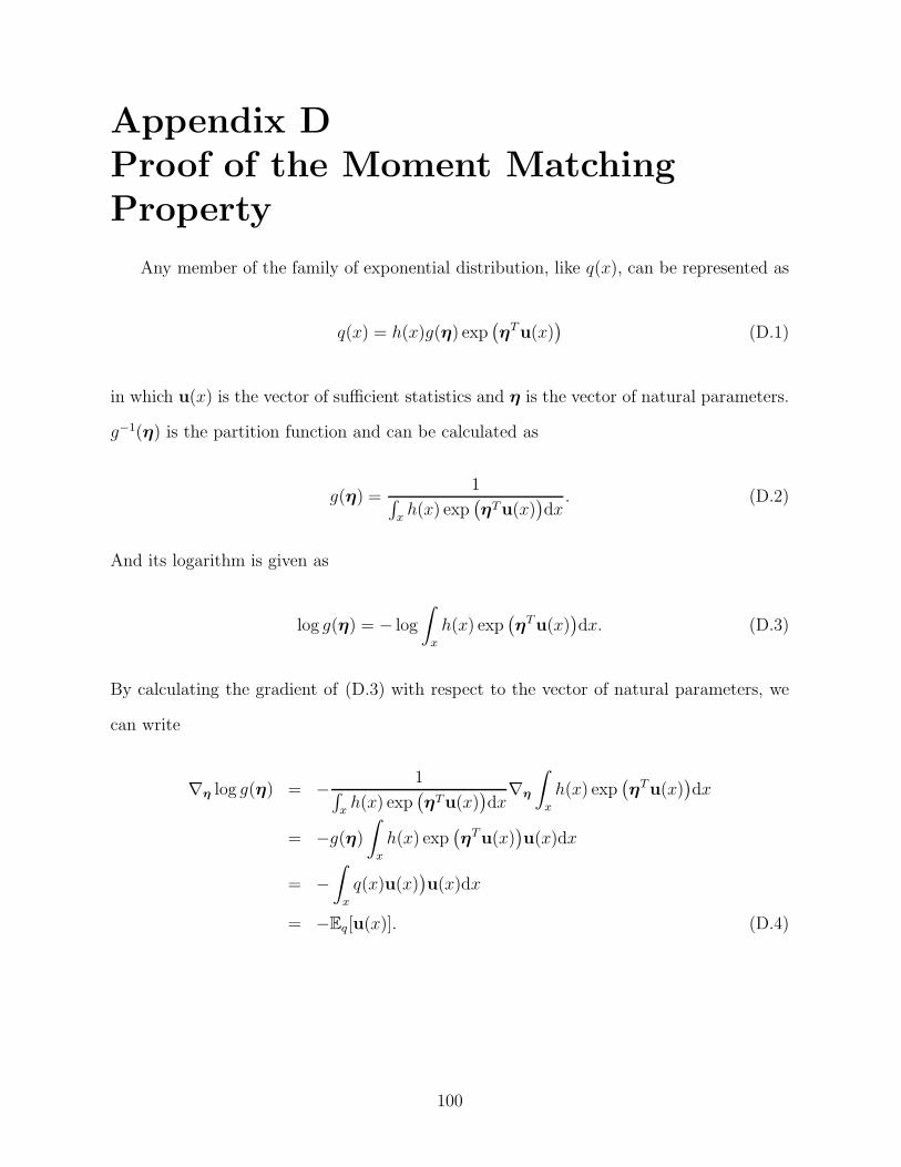
Appendix D
Proof of the Moment Matching
Property
Any member of the family of exponential distribution, like q(x), can be represented as
q(x) = h(x)g(η) exp(
ηTu(x))
(D.1)
in which u(x) is the vector of sufficient statistics and η is the vector of natural parameters.
g−1(η) is the partition function and can be calculated as
g(η) =1
∫
xh(x) exp
(
ηTu(x))
dx. (D.2)
And its logarithm is given as
log g(η) = − log
∫
x
h(x) exp(
ηTu(x))
dx. (D.3)
By calculating the gradient of (D.3) with respect to the vector of natural parameters, we
can write
∇η log g(η) = − 1∫
xh(x) exp
(
ηTu(x))
dx∇η
∫
x
h(x) exp(
ηTu(x))
dx
= −g(η)∫
x
h(x) exp(
ηTu(x))
u(x)dx
= −∫
x
q(x)u(x))
u(x)dx
= −Eq[u(x)]. (D.4)
100
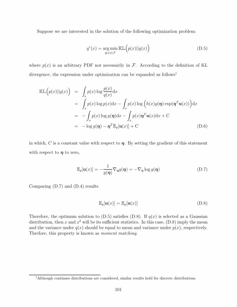
Suppose we are interested in the solution of the following optimization problem:
q∗(x) = argminq(x)∈F
KL
(
p(x)||q(x))
(D.5)
where p(x) is an arbitrary PDF not necessarily in F . According to the definition of KL
divergence, the expression under optimization can be expanded as follows1
KL
(
p(x)||q(x))
=
∫
x
p(x) logp(x)
q(x)dx
=
∫
x
p(x) log p(x)dx−∫
x
p(x) log(
h(x)g(η) exp(ηTu(x)))
dx
= −∫
x
p(x) log g(η)dx−∫
x
p(x)ηTu(x)dx+ C
= − log g(η)− ηTEp[u(x)] + C (D.6)
in which, C is a constant value with respect to η. By setting the gradient of this statement
with respect to η to zero,
Ep[u(x)] = − 1
g(η)∇ηg(η) = −∇η log g(η) (D.7)
Comparing (D.7) and (D.4) results
Eq[u(x)] = Ep[u(x)] (D.8)
Therefore, the optimum solution to (D.5) satisfies (D.8). If q(x) is selected as a Gaussiandistribution, then x and x2 will be its sufficient statistics. In this case, (D.8) imply the meanand the variance under q(x) should be equal to mean and variance under p(x), respectively.Threfore, this property is known as moment matching.
1Although continues distributions are considered, similar results hold for discrete distributions.
101
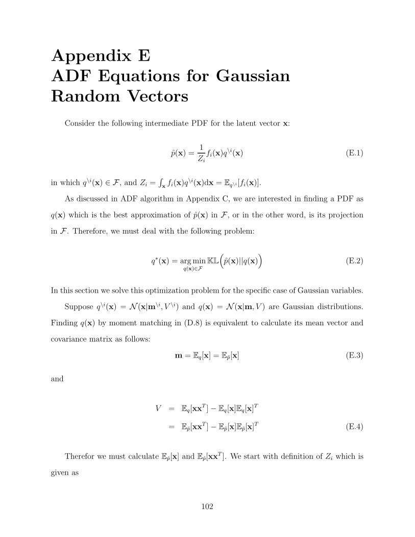
Appendix E
ADF Equations for Gaussian
Random Vectors
Consider the following intermediate PDF for the latent vector x:
p(x) =1
Zifi(x)q
\i(x) (E.1)
in which q\i(x) ∈ F , and Zi =∫
xfi(x)q
\i(x)dx = Eq\i[fi(x)].
As discussed in ADF algorithm in Appendix C, we are interested in finding a PDF as
q(x) which is the best approximation of p(x) in F , or in the other word, is its projection
in F . Therefore, we must deal with the following problem:
q∗(x) = argminq(x)∈F
KL
(
p(x)||q(x))
(E.2)
In this section we solve this optimization problem for the specific case of Gaussian variables.
Suppose q\i(x) = N (x|m\i, V \i) and q(x) = N (x|m, V ) are Gaussian distributions.
Finding q(x) by moment matching in (D.8) is equivalent to calculate its mean vector and
covariance matrix as follows:
m = Eq[x] = Ep[x] (E.3)
and
V = Eq[xxT ]− Eq[x]Eq[x]
T
= Ep[xxT ]− Ep[x]Ep[x]
T (E.4)
Therefor we must calculate Ep[x] and Ep[xxT ]. We start with definition of Zi which is
given as
102
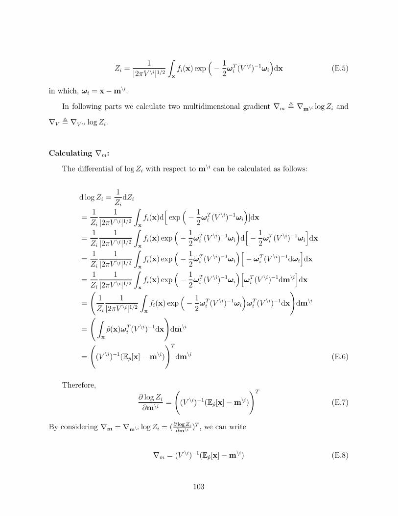
Zi =1
|2πV \i|1/2∫
x
fi(x) exp(
− 1
2ωT
i (V\i)−1ωi
)
dx (E.5)
in which, ωi = x−m\i.
In following parts we calculate two multidimensional gradient ∇m , ∇m\i logZi and
∇V , ∇V \i logZi.
Calculating ∇m:
The differential of logZi with respect to m\i can be calculated as follows:
d logZi =1
ZidZi
=1
Zi
1
|2πV \i|1/2∫
x
fi(x)d[
exp(
− 1
2ωT
i (V\i)−1ωi
)
]dx
=1
Zi
1
|2πV \i|1/2∫
x
fi(x) exp(
− 1
2ωT
i (V\i)−1ωi
)
d[
− 1
2ωT
i (V\i)−1ωi
]
dx
=1
Zi
1
|2πV \i|1/2∫
x
fi(x) exp(
− 1
2ωT
i (V\i)−1ωi
)[
− ωTi (V
\i)−1dωi
]
dx
=1
Zi
1
|2πV \i|1/2∫
x
fi(x) exp(
− 1
2ωT
i (V\i)−1ωi
)[
ωTi (V
\i)−1dm\i]
dx
=
(
1
Zi
1
|2πV \i|1/2∫
x
fi(x) exp(
− 1
2ωT
i (V\i)−1ωi
)
ωTi (V
\i)−1dx
)
dm\i
=
(
∫
x
p(x)ωTi (V
\i)−1dx
)
dm\i
=
(
(V \i)−1(Ep[x]−m\i)
)T
dm\i (E.6)
Therefore,
∂ logZi
∂m\i=
(
(V \i)−1(Ep[x]−m\i)
)T
(E.7)
By considering ∇m = ∇m\i logZi = (∂ logZi
∂m\i )T , we can write
∇m = (V \i)−1(Ep[x]−m\i) (E.8)
103

Finnaly, by (E.3) and (E.8),
m = Ep[x] = m\i + V \i∇m (E.9)
Calculating ∇V :
The differential of logZi with respect to V \i can be calculated as follows:
d logZi = d
(
log
∫
x
fi(x) exp(
− 1
2ωT
i (V\i)−1ωi
)
dx− 1
2log |2πV \i|
)
=1
Zi|2πV \i|1/2d(
∫
x
fi(x) exp(
− 1
2ωT
i (V\i)−1ωi
)
dx
)
−1
2tr(
(V \i)−1dV \i)
=1
Zi|2πV \i|1/2 ×∫
x
fi(x) exp(
− 1
2ωT
i (V\i)−1ωi
)
(1
2)tr(
(V \i)−1ωiωTi (V
\i)−1dV \i)
dx
−1
2tr(
(V \i)−1dV \i)
(E.10)
Therefore,
∂ logZi
∂V \i=
1
2
1
Zi|2πV \i|1/2∫
x
fi(x) exp(
− 1
2ωT
i (V\i)−1ωi
)
(V \i)−1ωiωTi (V
\i)−1dx
−1
2(V \i)−1
=1
2
∫
x
p(x)(V \i)−1ωiωTi (V
\i)−1dx− 1
2(V \i)−1
=1
2(V \i)−1
(
∫
x
p(x)(x−m\i)(x−m\i)Tdx
)
(V \i)−1 − 1
2(V \i)−1
=1
2(V \i)−1
(
Ep[xxT ]− Ep[x]m
\iT −m\iEp[x
T ] +m\im\iT
)
(V \i)−1
−1
2(V \i)−1 (E.11)
104
By considering ∇V = ∇V \i logZi = (∂ logZi
∂V \i )T , we can write
Ep[xxT ] = 2V \i∇V V
\i + Ep[x]m\iT +m\i
Ep[xT ]−m\im\iT + V \i (E.12)
By using (E.9) and plugging the equivalent expression of Ep[x], we can write
Ep[xxT ] = 2V \i∇V V
\i + (m\i + V \i∇m)m\iT +m\i(m\i + V \i∇m)
T
−m\im\iT + V \i (E.13)
By (E.4),
V = 2V \i∇V V\i + (m\i + V \i∇m)m
\iT +m\i(m\i + V \i∇m)T
−m\im\iT + V \i − (m\i + V \i∇m)(m\i + V \i∇m)
T
= 2V \i∇V V\i − V \i∇m∇T
mV\i + V \i (E.14)
which can finaly expressed as
V = V \i − V \i(∇m∇Tm − 2∇V )V
\i (E.15)
Equations (E.9) and (E.15) are known as ADF equations and are very useful in up-dating statistics of multidimensional Gaussian random variables in ADF or expectationpropagation algorithms.
105

Appendix F
Calculating Zt
The constant Zt can be calculated as follows:
Zt = Eq\t(S,h)[p(yt|st,h)]
=∑
s1,...,sT∈AKM
∫
q\t(S,h)p(yt|st,h)dh
=∑
s1,...,sT∈AKM
∫
q\t(S,h)p(yt|st,h)dh
=∑
s1,...,sT∈AKM
q\t(S)
∫
N(
h|m\th , V
\th
)
N(
yt|Sth,1
2σ′2wI2M
)
dh
=∑
s1,...,sT∈AKM
q\t(S)N(
yt|Stm\th , StV
\th S
Tt +
1
2σ′2wI2M
)
=∑
s1,...,sT∈AKM
T∏
i=1i 6=t
qi(si)
N(
yt|Stm\th , StV
\th S
Tt +
1
2σ′2wI2M
)
=
∑
s1,...,st−1,st+1,...,sT∈AKM
T∏
i=1i 6=t
qi(si)
∑
st∈AKM
N(
yt|Stm\th , StV
\th S
Tt +
1
2σ′2wI2M
)
=∑
st∈AKM
N(
yt|Stm\th , StV
\th S
Tt +
1
2σ′2wI2M
)
(F.1)
106
Appendix G
Hybrid K-L Divergence Optimization
Problem
Consider the following optimization problem on the hybrid K-L divergence:
minq(S,h)∈ F
KL(
pt(S,h)||q(S)q(h))
, (G.1)
in which, S = [s1, . . . , sT ] is a K × T matrix of discrete symbols in AM, i.e. S ∈ AK×TM ,
and h is the continues channel vector. By using the definition of K-L divergence, we can
write
KL(
pt(S,h)||q(S)q(h))
= Ept(S,h)
[
logpt(S,h)
q(S)q(h)
]
=∑
s1,...,sT∈AKM
∫
h
pt(S,h) logpt(S,h)
q(S)q(h)dh
=∑
s1,...,sT∈AKM
∫
h
pt(S,h) log pt(S,h)dh−
∑
s1,...,sT∈AKM
∫
h
pt(S,h) log(
q(S)q(h))
dh (G.2)
Since the optimization in (G.1) is over the functional q(S,h), the first term in (G.2) will
be a constant with respect to q(S,h) and can be replaced with letter C. Therefore we can
continue (G.2) as follows:
KL(
pt(S,h)||q(S)q(h))
= −∑
s1,...,sT∈AKM
∫
h
pt(S,h) log(
q(S)q(h))
dh+ C
= −∑
s1,...,sT∈AKM
∫
h
pt(S,h) log q(S)dh
−∑
s1,...,sT∈AKM
∫
h
pt(S,h) log q(h)dh+ C
107
= −∑
s1,...,sT∈AKM
log q(S)
∫
h
pt(S,h)dh
−∫
h
log q(h)(
∑
s1,...,sT∈AKM
pt(S,h))
dh+ C
= −∑
s1,...,sT∈AKM
pt(S) log q(S)
−∫
h
pt(h) log q(h)dh+ C (G.3)
in which,
pt(S) =
∫
h
pt(S,h)dh (G.4)
and
pt(h) =∑
s1,...,sT∈AKM
pt(S,h) (G.5)
are respective marginal distributions of S and h from pt(S,h).
By adding and subtracting two constant terms∑
s1,...,sT∈AKMpt(S) log pt(S) and
∫
hpt(h) log pt(h)dh to (G.3), we can write it as
KL(
pt(S,h)||q(S)q(h))
=∑
s1,...,sT∈AKM
pt(S) logpt(S)
q(S)+
∫
h
pt(h) logpt(h)
q(h)dh+ C ′
= KL(
pt(S)||q(S))
+KL(
pt(h)||q(h))
+ C ′ (G.6)
The first term in (G.6) totally depends on q(s) and the second term only depends
on q(S). Therefore the first two terms of (G.3) are changing independently. Therefore,
the minimization of (G.3) will be equivalent to minimization of both of these two terms.
Consequently, (G.1) can be broken into the following optimization problems:
qnew(S) = argminq(S)
KL(
pt(S)||q(S))
(G.7)
108

and
qnew(h) = argminq(h)
KL(
pt(h)||q(h))
(G.8)
109
VitaKamran Ghavami received his B.S. and M.S. degrees in electrical engineering from the
University of Tehran, Tehran, Iran, in 1998 and 2000, respectively. Upon the completion of
the M.S. degree, he conducted research and implementation of telecommunication systems
as a Research Engineer at NRI, where he participated in several related projects. In January
2013, he began working toward the Ph.D. degree with Louisiana State University, Baton
Rouge, LA, USA. His research interests include channel coding, iterative detection, and
multiple-input multiple-output wireless systems.
110