ch10 urban street concepts - againc.net · highway capacity manual 2000 10-i chapter 10 - urban...
TRANSCRIPT

Highway Capacity Manual 2000
10-i Chapter 10 - Urban Street Concepts
CHAPTER 10
URBAN STREET CONCEPTS
CONTENTS
I. INTRODUCTION..................................................................................................... 10-1II. URBAN STREETS .................................................................................................. 10-1
Flow Characteristics ......................................................................................... 10-3Free-Flow Speed ...................................................................................... 10-3Running Speed ......................................................................................... 10-3Travel Speed............................................................................................. 10-4Time-Space Trajectory .............................................................................. 10-4
Levels of Service .............................................................................................. 10-4Required Input Data and Estimated Values ..................................................... 10-5
Urban Street Class .................................................................................... 10-5Length ....................................................................................................... 10-7Free-Flow Speed ...................................................................................... 10-7Signal Density ........................................................................................... 10-8Peak-Hour Factor ...................................................................................... 10-8Length of Analysis Period ......................................................................... 10-8
Service Volume Table ...................................................................................... 10-9III. SIGNALIZED INTERSECTIONS............................................................................. 10-9
Signalized Intersection Flow Characteristics.................................................... 10-9Traffic Signal Characteristics.......................................................................... 10-14Saturation Flow Rate ...................................................................................... 10-15Signalized Intersection Capacity .................................................................... 10-15Level of Service .............................................................................................. 10-15Required Input Data and Estimated Values ................................................... 10-17
Lane Additions and Drops at Intersections ............................................. 10-17Exclusive Turn Lanes .............................................................................. 10-17
Exclusive Left-Turn Lanes ............................................................... 10-18Exclusive Right-Turn Lanes ............................................................. 10-18Number of Lanes ............................................................................. 10-18Other Features................................................................................. 10-18
Intersection Turning Movements............................................................. 10-19Default Values in Absence of Turning Movement Data ................... 10-19Turning Movement Estimation ......................................................... 10-19
Peak-Hour Factor .................................................................................... 10-21Length of Analysis Period ....................................................................... 10-21Intersection Control Type ........................................................................ 10-21Cycle Length ........................................................................................... 10-21Lost Time and Estimation of Signal Phasing .......................................... 10-22Effective Green Ratio .............................................................................. 10-23Arrival Type............................................................................................. 10-23Progression Adjustment Factor............................................................... 10-23Incremental Delay Adjustment ................................................................ 10-24Upstream Filtering/Metering Adjustment Factor ..................................... 10-24Base Saturation Flow Rate ..................................................................... 10-24Adjusted Saturation Flow Rates .............................................................. 10-24Lane Widths ............................................................................................ 10-24Heavy Vehicles ....................................................................................... 10-25Grades .................................................................................................... 10-25

Chapter 10 - Urban Street Concepts 10-ii
Parking Maneuvers ................................................................................. 10-25Local Buses ............................................................................................ 10-25Pedestrians ............................................................................................. 10-26Area Type ............................................................................................... 10-26Lane Utilization ....................................................................................... 10-26
Service Volume Table .................................................................................... 10-26IV. UNSIGNALIZED INTERSECTIONS...................................................................... 10-27
Characteristics of TWSC Intersections .......................................................... 10-27Flow at TWSC Intersections .......................................................................... 10-27Gap Acceptance Models ................................................................................ 10-28
Availability of Gaps ................................................................................. 10-28Usefulness of Gaps ................................................................................ 10-28Relative Priority of Various Streams at the Intersection.......................... 10-28
Capacity of TWSC Intersections .................................................................... 10-29Characteristics of AWSC Intersections .......................................................... 10-30Flow at AWSC Intersections .......................................................................... 10-30Characteristics of Roundabouts ..................................................................... 10-31Performance Measures .................................................................................. 10-31Required Input Data and Estimated Values ................................................... 10-32
Two-Way Stop-Controlled Intersections ................................................. 10-32Intersection Geometry ..................................................................... 10-32Control ............................................................................................. 10-32Volumes........................................................................................... 10-33
All-Way Stop-Controlled Intersections .................................................... 10-33Intersection Geometry ..................................................................... 10-33Volumes........................................................................................... 10-33
Roundabouts .......................................................................................... 10-34Intersection Geometry ..................................................................... 10-34Volumes........................................................................................... 10-34
Service Volume Tables .................................................................................. 10-34V. REFERENCES ...................................................................................................... 10-35APPENDIX A. QUICK ESTIMATION METHOD FOR
SIGNALIZED INTERSECTIONS......................................................... 10-36Input Requirements ........................................................................................ 10-36Determination of Left-Turn Treatment ............................................................ 10-37Lane Volume Computations........................................................................... 10-42Signal Timing Estimation................................................................................ 10-43
Phasing Plan Development .................................................................... 10-43Computation of Critical Sum ................................................................... 10-44Estimation of Total Lost Time ................................................................. 10-45Cycle Length Estimation ......................................................................... 10-45Green Time Estimation ........................................................................... 10-45
Computation of Critical v/c Ratio .................................................................... 10-46Computation of Delay .................................................................................... 10-47
APPENDIX B. WORKSHEETS................................................................................... 10-47Quick Estimation Input WorksheetLeft-Turn Treatment WorksheetQuick Estimation Lane Volume WorksheetQuick Estimation Control Delay and LOS Worksheet
Highway Capacity Manual 2000

Highway Capacity Manual 2000
10-iii Chapter 10 - Urban Street Concepts
EXHIBITS
Exhibit 10-1. Typical Speed Profiles of Vehicles on Urban Streets............................ 10-4Exhibit 10-2. Required Input Data for Urban Streets.................................................. 10-5Exhibit 10-3. Urban Street Class Based on Functional and Design Categories......... 10-6Exhibit 10-4. Functional and Design Categories ........................................................ 10-6Exhibit 10-5. Free-Flow Speed by Urban Street Class............................................... 10-8Exhibit 10-6. Signal Density by Urban Street Class ................................................... 10-8Exhibit 10-7. Example Service Volumes for Urban Streets ...................................... 10-10Exhibit 10-8. Fundamental Attributes of Flow at Signalized Intersections ............... 10-11Exhibit 10-9. Symbols, Definitions, and Units for Fundamental Variables of
Traffic Flow at Signalized Intersections ............................................... 10-12Exhibit 10-10. Relationship Among Actual Green, Lost-Time Elements,
Extension of Effective Green, and Effective Green ............................. 10-13Exhibit 10-11. Lost Time Application for Compound Left-Turn Phasing..................... 10-14Exhibit 10-12. Required Data for Signalized Intersections ......................................... 10-17Exhibit 10-13. Turn Volumes Probably Requiring Exclusive Left-Turn Lanes at
Signalized Intersections ...................................................................... 10-18Exhibit 10-14. Origin-Destination Labels for Intersection Turning Movements .......... 10-19Exhibit 10-15. Intersection Control Type and Peak-Hour Volumes ............................ 10-21Exhibit 10-16. Default Cycle Lengths by Area Type ................................................... 10-21Exhibit 10-17. Default Lost Time per Cycle by Left Phase Type ................................ 10-22Exhibit 10-18. Progression Quality and Arrival Type.................................................. 10-23Exhibit 10-19. Adjusted Saturation Flow Rate by Area Type ..................................... 10-24Exhibit 10-20. Parking Maneuver Defaults ................................................................. 10-25Exhibit 10-21. Bus Frequency Defaults ...................................................................... 10-25Exhibit 10-22. Defaults for Pedestrian Flows.............................................................. 10-26Exhibit 10-23. Default Lane Utilization Adjustment Factors ....................................... 10-26Exhibit 10-24. Example Service Volumes for Signalized Intersection ........................ 10-27Exhibit 10-25. Analysis Cases for AWSC Intersections.............................................. 10-30Exhibit 10-26. Basic Roundabout Geometrics ............................................................ 10-32Exhibit 10-27. Minimum Approach Volumes (veh/h) for Left-Turn Lanes on Two-
Lane Highways at Unsignalized Intersections ..................................... 10-33Exhibit 10-28. Example of Minor Street Service Volumes for T-Intersection
Two-Way Stop Intersection ................................................................. 10-34Exhibit 10-29. Example of Minor Street Service Volumes for Four-Leg
Intersection, Two-Way Stop ................................................................ 10-35Exhibit 10-30. Example of Approach Service Volumes for All-Way Stop
Intersections for Single Approach........................................................ 10-35Exhibit A10-1. Input Data Requirements for Quick Estimation Method ...................... 10-37Exhibit A10-2. Quick Estimation Input Worksheet ...................................................... 10-38Exhibit A10-3. Left-Turn Treatment Worksheet .......................................................... 10-39Exhibit A10-4. Quick Estimation Lane Volume Worksheet ......................................... 10-40Exhibit A10-5. Quick Estimation Control Delay and LOS Worksheet ......................... 10-41Exhibit A10-6. Shared-Lane, Left-Turn Adjustment Computation for
Quick Estimation.................................................................................. 10-43Exhibit A10-7. Phase Plans for Quick Estimation Method .......................................... 10-44Exhibit A10-8. Phase Plan Summary for Quick Estimation Method ........................... 10-44Exhibit A10-9. Intersection Status Criteria for Signalized Intersection
Planning Analysis ................................................................................ 10-46
Highway Capacity Manual 2000
10-1 Chapter 10 - Urban Street ConceptsIntroduction
I. INTRODUCTION
In this chapter, capacity and quality of service concepts for urban streets areintroduced. The term “urban streets,” as used in this manual, refers to urban arterials andcollectors, including those in downtown areas. Methodologies found in Chapter 15(Urban Streets), Chapter 16 (Signalized Intersections), and Chapter 17 (UnsignalizedIntersections) can be used in conjunction with this chapter.
II. URBAN STREETS
In the hierarchy of street transportation facilities, urban streets (including arterialsand collectors) are ranked between local streets and multilane suburban and ruralhighways. The difference is determined principally by street function, control conditions,and the character and intensity of roadside development.
Arterial streets are roads that primarily serve longer through trips. However,providing access to abutting commercial and residential land uses is also an importantfunction of arterials. Collector streets provide both land access and traffic circulationwithin residential, commercial, and industrial areas. Their access function is moreimportant than that of arterials, and unlike arterials their operation is not alwaysdominated by traffic signals.
Downtown streets are signalized facilities that often resemble arterials. They notonly move through traffic but also provide access to local businesses for passenger cars,transit buses, and trucks. Turning movements at downtown intersections are often greaterthan 20 percent of total traffic volume because downtown flow typically involves asubstantial amount of circulatory traffic.
Pedestrian conflicts and lane obstructions created by stopping or standing taxicabs,buses, trucks, and parking vehicles that cause turbulence in the traffic flow are typical ofdowntown streets. Downtown street function may change with the time of day; somedowntown streets are converted to arterial-type operation during peak traffic hours.
Multilane suburban and rural highways differ from urban streets in the followingways: roadside development is not as intense, density of traffic access points is not ashigh, and signalized intersections are more than 3.0 km apart. These conditions result ina smaller number of traffic conflicts, smoother flow, and dissipation of the platoonstructure associated with traffic flow on an arterial or collector with traffic signals.
The urban streets methodology described in this chapter and in Chapter 15 can beused to assess the mobility function of the urban street. The degree of mobility providedis assessed in terms of travel speed for the through-traffic stream. A street’s accessfunction is not assessed by this methodology. The level of access provided by a streetshould also be considered in evaluating its performance, especially if the street isintended to provide such access. Oftentimes, factors that favor mobility reflect minimallevels of access and vice versa.
Functional class definedThe functional classification of an urban street is the type of traffic service the streetprovides. Within the functional classification, the arterial is further classified by itsdesign category. Illustrations 10-1 through 10-4 show typical examples of four designcategories that are described in the following sections.

Highway Capacity Manual 2000
Chapter 10 - Urban Street Concepts 10-2Urban Streets
ILLUSTRATION 10-1. Typical high-speed design.
ILLUSTRATION 10-2. Typical suburban design.
ILLUSTRATION 10-3. Typical intermediate design.

Highway Capacity Manual 2000
10-3 Chapter 10 - Urban Street ConceptsUrban Streets
ILLUSTRATION 10-4. Typical urban design.
FLOW CHARACTERISTICS
The speed of vehicles on urban streets is influenced by three main factors: streetenvironment, interaction among vehicles, and traffic control. As a result, these factorsalso affect quality of service.
The street environment includes the geometric characteristics of the facility, thecharacter of roadside activity, and adjacent land uses. Thus, the environment reflects thenumber and width of lanes, type of median, driveway/access-point density, spacingbetween signalized intersections, existence of parking, level of pedestrian activity, andspeed limit.
The interaction among vehicles is determined by traffic density, the proportion oftrucks and buses, and turning movements. This interaction affects the operation ofvehicles at intersections and, to a lesser extent, between signals.
Traffic control (including signals and signs) forces a portion of all vehicles to slow orstop. The delays and speed changes caused by traffic control devices reduce vehiclespeeds; however, such controls are needed to establish right-of-way.
Free-Flow Speed
The street environment affects the driver’s speed choice. When vehicle interactionand traffic control are not factors, the speed chosen by the average driver is referred to asthe free-flow speed (FFS). FFS is the average speed of the traffic stream when trafficvolumes are sufficiently low that drivers are not influenced by the presence of othervehicles and when intersection traffic control (i.e., signal or sign) is not present or issufficiently distant as to have no effect on speed choice. As a consequence, FFS istypically observed along midblock portions of the urban street segment.
Running Speed
A driver can seldom travel at the FFS. Most of the time, the presence of othervehicles restricts the speed of a vehicle in motion because of differences in speeds amongdrivers or because downstream vehicles are accelerating from a stop and have not yetreached FFS. As a result, vehicle speeds tend to be lower than the FFS during moderateto high-volume conditions.
One speed characteristic that captures the effect of interaction among vehicles is theaverage running speed. This speed is computed as the length of the segment divided bythe average running time. The running time is the time taken to traverse the streetsegment, less any stop-time delay.
Highway Capacity Manual 2000
Chapter 10 - Urban Street Concepts 10-4Urban Streets
Travel Speed
The presence of traffic control on a street segment tends to reduce vehicle speedsbelow the average running speed. A speed characteristic that captures the effect of trafficcontrol is average travel speed. This speed is computed as the length of segment dividedby the average travel time. The travel time is the time taken to traverse the streetsegment, inclusive of any stop-time delay.
Time-Space Trajectory
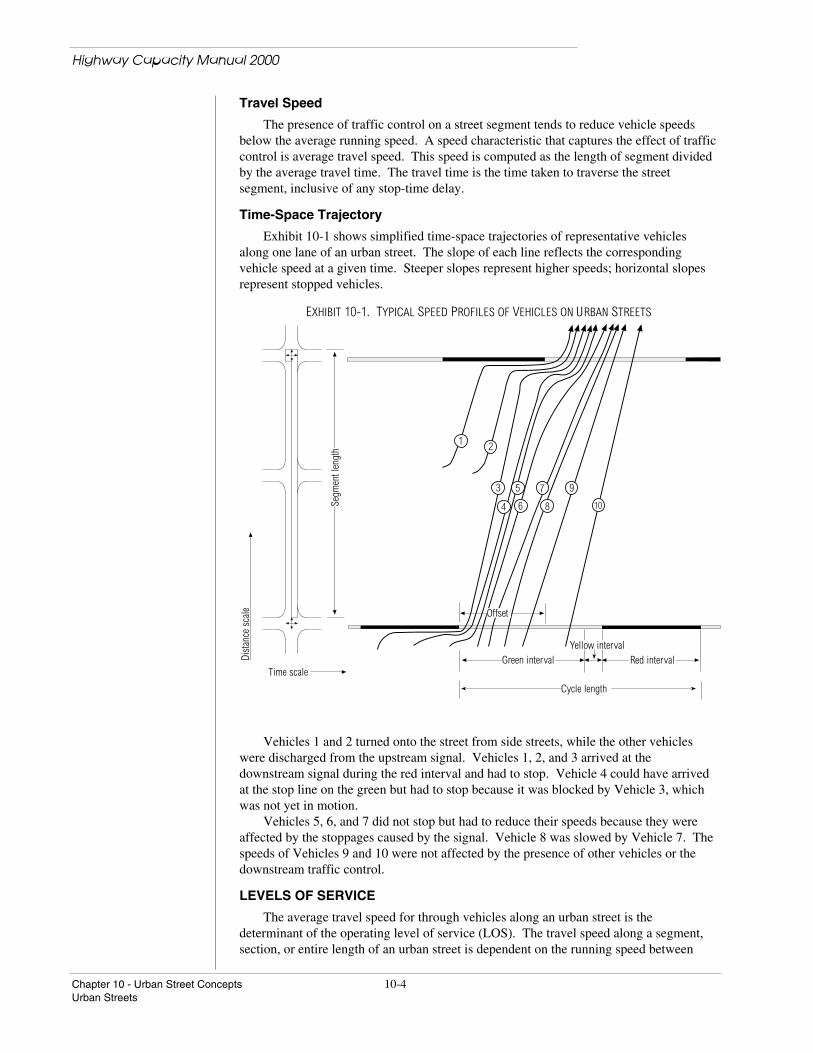
Exhibit 10-1 shows simplified time-space trajectories of representative vehiclesalong one lane of an urban street. The slope of each line reflects the correspondingvehicle speed at a given time. Steeper slopes represent higher speeds; horizontal slopesrepresent stopped vehicles.
EXHIBIT 10-1. TYPICAL SPEED PROFILES OF VEHICLES ON URBAN STREETS
1 2
Segm
ent l
engt
h
Time scale
Dist
ance
sca
le
Red interval
Cycle length
Green interval
10
97
86
5
4
3
Offset
Yellow interval
Vehicles 1 and 2 turned onto the street from side streets, while the other vehicleswere discharged from the upstream signal. Vehicles 1, 2, and 3 arrived at thedownstream signal during the red interval and had to stop. Vehicle 4 could have arrivedat the stop line on the green but had to stop because it was blocked by Vehicle 3, whichwas not yet in motion.
Vehicles 5, 6, and 7 did not stop but had to reduce their speeds because they wereaffected by the stoppages caused by the signal. Vehicle 8 was slowed by Vehicle 7. Thespeeds of Vehicles 9 and 10 were not affected by the presence of other vehicles or thedownstream traffic control.
LEVELS OF SERVICE
The average travel speed for through vehicles along an urban street is thedeterminant of the operating level of service (LOS). The travel speed along a segment,section, or entire length of an urban street is dependent on the running speed between
Highway Capacity Manual 2000
10-5 Chapter 10 - Urban Street ConceptsUrban Streets
signalized intersections and the amount of control delay incurred at signalizedintersections.
LOS is based on averagethrough-vehicle travel speedfor the urban street segment
Urban street LOS is based on average through-vehicle travel speed for the segment,section, or entire urban street under consideration. The following general statementscharacterize LOS along urban streets. Refer to Exhibit 15-2 for speed ranges for eachLOS.
LOS A describes primarily free-flow operations at average travel speeds, usuallyabout 90 percent of the FFS for the given street class. Vehicles are completelyunimpeded in their ability to maneuver within the traffic stream. Control delay atsignalized intersections is minimal.
LOS B describes reasonably unimpeded operations at average travel speeds, usuallyabout 70 percent of the FFS for the street class. The ability to maneuver within the trafficstream is only slightly restricted, and control delays at signalized intersections are notsignificant.
LOS C describes stable operations; however, ability to maneuver and change lanes inmidblock locations may be more restricted than at LOS B, and longer queues, adversesignal coordination, or both may contribute to lower average travel speeds of about 50percent of the FFS for the street class.
LOS D borders on a range in which small increases in flow may cause substantialincreases in delay and decreases in travel speed. LOS D may be due to adverse signalprogression, inappropriate signal timing, high volumes, or a combination of these factors.Average travel speeds are about 40 percent of FFS.
LOS E is characterized by significant delays and average travel speeds of 33 percentor less of the FFS. Such operations are caused by a combination of adverse progression,high signal density, high volumes, extensive delays at critical intersections, andinappropriate signal timing.
LOS F is characterized by urban street flow at extremely low speeds, typically one-third to one-fourth of the FFS. Intersection congestion is likely at critical signalizedlocations, with high delays, high volumes, and extensive queuing.
REQUIRED INPUT DATA AND ESTIMATED VALUES
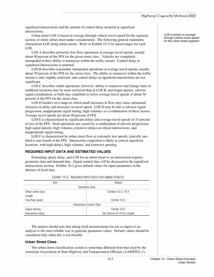
Estimating speed, delay, and LOS for an urban street or an intersection requiresgeometric data and demand data. Signal control data will be discussed in the signalizedintersections section. Exhibit 10-2 gives default values for input parameters in theabsence of local data.
EXHIBIT 10-2. REQUIRED INPUT DATA FOR URBAN STREETS
Item Default
Geometric Data
Urban street class Exhibits 10-3, 10-4Length -Free-flow speed Exhibit 10-5
Intersection Control Data
Signal density Exhibit 10-6Intersection delay See Section III of this chapter
The analyst should note that taking field measurements for use as inputs to ananalysis is the most reliable way to generate parameter values. Default values should beconsidered only when this is not feasible.
Urban Street Class
The urban street classification system is somewhat different from that used by theAmerican Association of State Highway and Transportation Officials (AASHTO) (1).
Highway Capacity Manual 2000
Chapter 10 - Urban Street Concepts 10-6Urban Streets
AASHTO’s functional classes are based on travel volume, mileage, and the characteristicof service the urban street is intended to provide. The analysis method in this manualmakes use of the AASHTO distinction between principal arterial and minor arterial. Buta second classification step is used herein to determine the appropriate design categoryfor the arterial. The design category depends on the posted speed limit, signal density,driveway/access-point density, and other design features. The third step is to determinethe appropriate urban street class on the basis of a combination of functional category anddesign category. Exhibits 10-3 and 10-4 are useful for establishing urban street class.
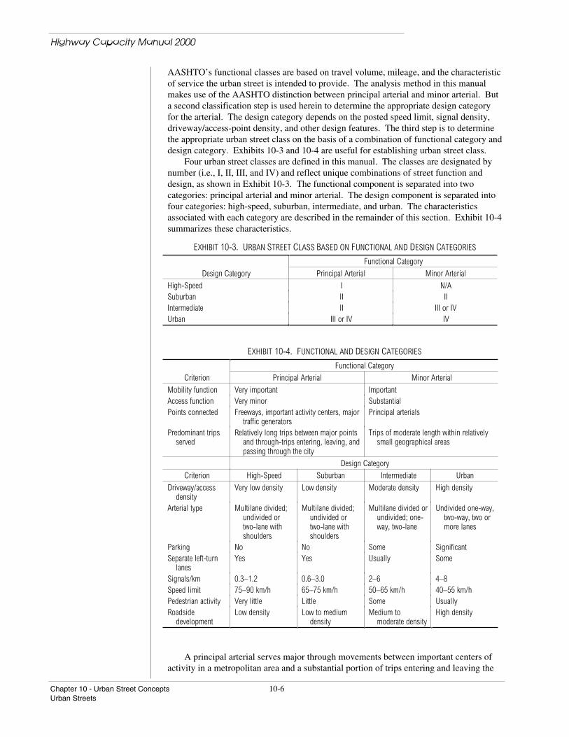
Four urban street classes are defined in this manual. The classes are designated bynumber (i.e., I, II, III, and IV) and reflect unique combinations of street function anddesign, as shown in Exhibit 10-3. The functional component is separated into twocategories: principal arterial and minor arterial. The design component is separated intofour categories: high-speed, suburban, intermediate, and urban. The characteristicsassociated with each category are described in the remainder of this section. Exhibit 10-4summarizes these characteristics.
EXHIBIT 10-3. URBAN STREET CLASS BASED ON FUNCTIONAL AND DESIGN CATEGORIES
Functional Category
Design Category Principal Arterial Minor Arterial
High-Speed I N/ASuburban II IIIntermediate II III or IVUrban III or IV IV
EXHIBIT 10-4. FUNCTIONAL AND DESIGN CATEGORIES
Functional Category
Criterion Principal Arterial Minor Arterial
Mobility function Very important ImportantAccess function Very minor SubstantialPoints connected Freeways, important activity centers, major
traffic generatorsPrincipal arterials
Predominant tripsserved
Relatively long trips between major pointsand through-trips entering, leaving, andpassing through the city
Trips of moderate length within relativelysmall geographical areas
Design Category
Criterion High-Speed Suburban Intermediate Urban
Driveway/accessdensity
Very low density Low density Moderate density High density
Arterial type Multilane divided;undivided ortwo-lane withshoulders
Multilane divided;undivided ortwo-lane withshoulders
Multilane divided orundivided; one-way, two-lane
Undivided one-way,two-way, two ormore lanes
Parking No No Some SignificantSeparate left-turn
lanesYes Yes Usually Some
Signals/km 0.3–1.2 0.6–3.0 2–6 4–8Speed limit 75–90 km/h 65–75 km/h 50–65 km/h 40–55 km/hPedestrian activity Very little Little Some UsuallyRoadside
developmentLow density Low to medium
densityMedium to
moderate densityHigh density
A principal arterial serves major through movements between important centers ofactivity in a metropolitan area and a substantial portion of trips entering and leaving the

Highway Capacity Manual 2000
10-7 Chapter 10 - Urban Street ConceptsUrban Streets
area. It also connects freeways with major traffic generators. In smaller cities(population under 50,000), its importance is derived from the service provided to trafficpassing through the urban area. Service to abutting land is subordinate to the function ofmoving through traffic.
A minor arterial connects and augments the principal arterial system. Although itsmain function is traffic mobility, it performs this function at a lower level and placesmore emphasis on land access than does the principal arterial. A system of minorarterials serves trips of moderate length and distributes travel to geographical areassmaller than those served by the principal arterial.
The urban street is further classified by its design category. Exhibit 10-3 showsurban street classes based on functional and design categories.
High-speed design definedHigh-speed design represents an urban street with a very low driveway/access-pointdensity, separate left-turn lanes, and no parking. It may be multilane divided orundivided or a two-lane facility with shoulders. Signals are infrequent and spaced at longdistances. Roadside development is low density, and the speed limit is typically 75 to 90km/h. This design category includes many urban streets in suburban settings.
Suburban design definedSuburban design represents a street with a low driveway/access-point density,separate left-turn lanes, and no parking. It may be multilane divided or undivided or atwo-lane facility with shoulders. Signals are spaced for good progressive movement (upto three signals per kilometer). Roadside development is low to medium density, andspeed limits are usually 65 to 75 km/h.
Intermediate design definedIntermediate design represents an urban street with a moderate driveway/access-pointdensity. It may be a multilane divided, an undivided one-way, or a two-lane facility. Itmay have some separate or continuous left-turn lanes and some portions where parking ispermitted. It has a higher density of roadside development than the typical suburbandesign and usually has two to six signals per kilometer. Speed limits are typically 50 to65 km/h.
Urban design definedUrban design represents an urban street with a high driveway/access-point density. Itfrequently is an undivided one-way or two-way facility with two or more lanes. Parkingis usually permitted. Generally, there are few separate left-turn lanes, and somepedestrian interference is present. It commonly has four to eight signals per kilometer.Roadside development is dense with commercial uses. Speed limits range from 40 to 55km/h.
In addition to the above definitions, Exhibit 10-4 can be used as an aid in thedetermination of functional and design categories. Once the functional and designcategories have been determined, the urban street classification may be established byreferring to Exhibit 10-3.
In practice, there are sometimes ambiguities in determining the proper categories.The measurement or estimation of the free-flow speed is a great aid in this determination,because each urban street class has a characteristic range of free-flow speeds, as shown inChapter 15.
Length
The portion of the urban street being analyzed should be at least 1.5 km long in adowntown area and 3.0 km long elsewhere for the LOS speed criteria to be meaningful.Study lengths shorter than 1.5 km should be analyzed as individual intersections and theLOS assessed according to individual intersection criteria.
Free-Flow SpeedMeasure free-flow speed asfar as possible from nearestsignal or stop-controlledintersection and at flows < 200veh/h/ln
The free-flow speed is used to determine the urban street class and to estimate thesegment running time. If FFS cannot be measured in the field, the analyst should attemptto take measurements on a similar facility in the same area or should resort to establishedlocal policies. Lacking any of these options, the analyst might rely on the posted speedlimit (or some value around that limit) or on default values in this manual.

Highway Capacity Manual 2000
Chapter 10 - Urban Street Concepts 10-8Urban Streets
Free-flow speed on an urban street is the speed that a vehicle travels under low-volume conditions when all the signals on the urban street are green for the entire trip.Thus, all delay at signalized intersections, even under low flow conditions, is excludedfrom the computation of urban street FFS. The best location to measure urban street FFSis midblock and as far as possible from the nearest signalized or stop-controlledintersection. This measurement should be made under low flow conditions (less than 200veh/h/ln). Exhibit 10-5 gives default FFS by urban street class for use in the absence oflocal data.
EXHIBIT 10-5. FREE-FLOW SPEED BY URBAN STREET CLASS
Urban Street Class Default (km/h)
I 80II 65III 55IV 45
Signal DensitySignal density defined Signal density is the number of signalized intersections in the study portion of the
urban street divided by its length. If signalized intersections are used to define both thebeginning and the ending points of the study portion of the urban street, then the numberof signals in the study portion should be reduced by one in computing the signal density.Exhibit 10-6 gives defaults by urban street class that may be used in the absence of localdata.
EXHIBIT 10-6. SIGNAL DENSITY BY URBAN STREET CLASS
Urban Street Class Default (signals/km)
I 0.5II 2III 4IV 6
Peak-Hour Factor
In the absence of field measurements of peak-hour factor (PHF), approximations canbe used. For congested conditions, 0.92 is a reasonable approximation for PHF. Forconditions in which there is fairly uniform flow throughout the peak hour but arecognizable peak does occur, 0.88 is a reasonable estimate for PHF.
Length of Analysis Period
The analytical procedures for estimating speed for an urban street depend on theestimation of delay for the signalized and unsignalized intersections on the street. Thedelay equations for signalized and unsignalized intersections are most accurate when thedemand is less than capacity for the selected analysis period. If the demand exceedscapacity, the intersection delay equations will estimate the delay for all vehicles arrivingduring the analysis period but will not determine the effect of the excess demand (theresidual queue for the next period) on the vehicles arriving during the next analysisperiod.
The typical analysis period is 15 min. However, if demand creates a residual queuefor the 15-min analysis period (i.e., v/c greater than 1.00), the analyst should consider theuse of multiple analysis periods or a single longer analysis period to improve the delayestimate.
Highway Capacity Manual 2000
10-9 Chapter 10 - Urban Street ConceptsUrban Streets
If a multiple-period analysis is selected, the analyst must carry over the residualqueue from one period to the next as discussed in Chapter 16, Appendix F (Extension ofSignal Delay Models to Incorporate the Effect of an Initial Queue). The analyst will haveto modify or adapt these procedures in the case of unsignalized intersections. Speed,delay, and LOS can then be computed for each analysis period. The analyst mustdetermine how to report these results, since averaging LOS across multiple analysisperiods may obscure some of the results.
If a single longer analysis period is selected (such as 1 h), the analyst should usecaution in performing the analysis and interpreting the results. The peak-hour factor(which normally is used to compute the peak 15-min flow rate from a 1-h volume) mayhave to be modified to provide the appropriate flow rate for the longer analysis period.The analyst must also recognize that LOS criteria for urban streets, signalizedintersections, and unsignalized intersections were developed for a 15-min analysis period.Conditions that persist for longer periods (presumably with worse peak conditions withinthose periods) may no longer meet the 15-min LOS criteria provided in this manual.
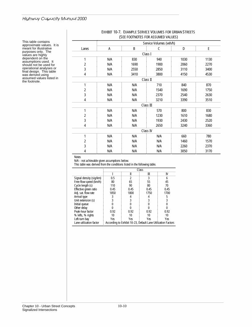
SERVICE VOLUME TABLE
Exhibit 10-7 is an example service volume table for the four urban street classes.This table is useful for estimates of how many vehicles an urban street can carry at agiven level of service, for a particular class and number of lanes (per direction). It ismost accurate when the defaults shown in Exhibit 10-7 are applicable. If conditions on agiven street vary considerably from those used to create this table, the tabular values arenot appropriate.
III. SIGNALIZED INTERSECTIONS
The capacity of an urban street is related primarily to the signal timing and thegeometric characteristics of the facility as well as to the composition of traffic on thefacility. Geometrics are a fixed characteristic of a facility. Thus, while trafficcomposition may vary somewhat over time, the capacity of a facility is generally a stablevalue that can be significantly improved only by initiating geometric improvements.
At signalized intersections, the additional element of time allocation is introducedinto the concept of capacity. A traffic signal essentially allocates time among conflictingtraffic movements that seek to use the same space. The way in which time is allocatedsignificantly affects the operation and the capacity of the intersection and its approaches.
Lane group definedIn analyzing a signalized intersection, the physical unit of analysis is the lane group.A lane group consists of one or more lanes on an intersection approach. The outputsfrom application of the method in this manual are reported on the basis of each lanegroup.
SIGNALIZED INTERSECTION FLOW CHARACTERISTICS
For a given lane group at a signalized intersection, three signal indications aredisplayed: green, yellow, and red. The red indication may include a short period duringwhich all indications are red, referred to as an all-red interval, which with the yellowindication forms the change and clearance interval between two green phases.
Exhibit 10-8 provides a reference for much of the discussion in this section. Itpresents some fundamental attributes of flow at signalized intersections. The diagramrepresents a simple situation of a one-way approach to a signalized intersection havingtwo phases in the cycle.
Chapter 10 - Urban Street Concepts 10-10Signalized Intersections
EXHIBIT 10-7. EXAMPLE SERVICE VOLUMES FOR URBAN STREETS(SEE FOOTNOTES FOR ASSUMED VALUES)
This table containsapproximate values. It ismeant for illustrativepurposes only. Thevalues are highlydependent on theassumptions used. Itshould not be used foroperational analyses orfinal design. This tablewas derived usingassumed values listed inthe footnote.
Service Volumes (veh/h)
Lanes A B C D E
Class I
1 N/A 830 940 1030 11302 N/A 1690 1900 2060 22703 N/A 2550 2850 3110 34004 N/A 3410 3800 4150 4530
Class II
1 N/A N/A 710 840 8702 N/A N/A 1540 1690 17503 N/A N/A 2370 2540 26304 N/A N/A 3210 3390 3510
Class III
1 N/A N/A 570 800 8302 N/A N/A 1230 1610 16803 N/A N/A 1930 2430 25204 N/A N/A 2650 3240 3360
Class IV
1 N/A N/A N/A 660 7802 N/A N/A N/A 1460 15703 N/A N/A N/A 2260 23704 N/A N/A N/A 3050 3170
NotesN/A - not achievable given assumptions below.This table was derived from the conditions listed in the following table.
ClassI II III IV
Signal density (sig/km) 0.5 2 3 6Free-flow speed (km/h) 80 65 55 45Cycle length (s) 110 90 80 70Effective green ratio 0.45 0.45 0.45 0.45Adj. sat. flow rate 1850 1800 1750 1700Arrival type 3 4 4 5Unit extension (s) 3 3 3 3Initial queue 0 0 0 0Other delay 0 0 0 0Peak-hour factor 0.92 0.92 0.92 0.92% lefts, % rights 10 10 10 10Left-turn bay Yes Yes Yes YesLane utilization factor According to Exhibit 10-23, Default Lane Utilization Factors
Highway Capacity Manual 2000

Highway Capacity Manual 2000
10-11 Chapter 10 - Urban Street ConceptsSignalized Intersections
EXHIBIT 10-8. FUNDAMENTAL ATTRIBUTES OF FLOW AT SIGNALIZED INTERSECTIONS
Red
Control delay forVeh. #2
Dist
ance
Time
Veh.
#0
Veh.
#1
Veh.
#2
Veh.
#3
Veh.
#4
Veh.
#5
Veh.
#6
Veh.
#7
Ci
Yi Ri Gi
gi
l1l2 e
Yi
l2
ri
Assumed periodof saturation flow
Flow
rate
Saturation flowrate
Equal areas
Veh.
#1
1
2
3
Green
Effective red Effective green
The exhibit is divided into three parts. The first part shows a time-space plot ofvehicles on the northbound approach to the intersection. The intervals for the signalcycle are indicated in the diagram. The second part repeats the timing intervals and labelsthe various time intervals of interest with the symbols used throughout this chapter. Thethird part is an idealized plot of flow rate passing the stop line, indicating how saturationflow is defined. Further definitions of these variables and other basic terms are providedin Exhibit 10-9.
Effective green definedEffective red defined
The signal cycle for a given lane group has two simplified components: effectivegreen and effective red. Effective green time is the time that may be used by vehicles onthe subject lane group at the saturation flow rate. Effective red time is defined as thecycle length minus the effective green time.
It is important that the relationship between the actual green, yellow, and red timesshown on signal faces and the effective green and red times be understood. Each time amovement is started and stopped, two lost times are experienced. At the beginning ofmovement, the first several vehicles in the queue experience start-up losses that result inmovement at less than the saturation flow rate (Exhibit 10-8). At the end of a movement,a portion of the change and clearance interval (yellow and all-red) is not used forvehicular movement.
Highway Capacity Manual 2000
Chapter 10 - Urban Street Concepts 10-12Signalized Intersections
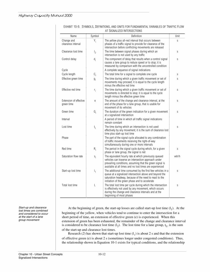
EXHIBIT 10-9. SYMBOLS, DEFINITIONS, AND UNITS FOR FUNDAMENTAL VARIABLES OF TRAFFIC FLOWAT SIGNALIZED INTERSECTIONS
Name Symbol Definition Unit
Change andclearance interval
Yi The yellow plus all-red interval that occurs betweenphases of a traffic signal to provide for clearance of theintersection before conflicting movements are released
s
Clearance lost time l2 The time between signal phases during which anintersection is not used by any traffic
s
Control delay di The component of delay that results when a control signalcauses a lane group to reduce speed or to stop; it ismeasured by comparison with the uncontrolled condition
s
Cycle A complete sequence of signal indicationsCycle length Ci The total time for a signal to complete one cycle s
Effective green time gi The time during which a given traffic movement or set ofmovements may proceed; it is equal to the cycle lengthminus the effective red time
s
Effective red time ri The time during which a given traffic movement or set ofmovements is directed to stop; it is equal to the cyclelength minus the effective green time
s
Extension of effectivegreen time
e The amount of the change and clearance interval, at theend of the phase for a lane group, that is usable formovement of its vehicles
s
Green time Gi The duration of the green indication for a given movementat a signalized intersection
s
Interval A period of time in which all traffic signal indicationsremain constant
Lost time tL The time during which an intersection is not usedeffectively by any movement; it is the sum of clearance losttime plus start-up lost time
s
Phase The part of the signal cycle allocated to any combinationof traffic movements receiving the right-of-waysimultaneously during one or more intervals
Red time Ri The period in the signal cycle during which, for a givenphase or lane group, the signal is red
s
Saturation flow rate si The equivalent hourly rate at which previously queuedvehicles can traverse an intersection approach underprevailing conditions, assuming that the green signal isavailable at all times and no lost times are experienced
veh/h
Start-up lost time l1 The additional time consumed by the first few vehicles in aqueue at a signalized intersection above and beyond thesaturation headway, because of the need to react to theinitiation of the green phase and to accelerate
s
Total lost time L The total lost time per cycle during which the intersectionis effectively not used by any movement, which occursduring the change and clearance intervals and at thebeginning of most phases
s
Start-up and clearancelost times are combinedand considered to occurat the start of a lanegroup movement
At the beginning of green, the start-up losses are called start-up lost time (l1). At the
beginning of the yellow, when vehicles tend to continue to enter the intersection for ashort period of time, an extension of effective green (e) is experienced. When thisextension of green has been exhausted, the remainder of the change and clearance intervalis considered to be clearance lost time (l2). The lost time for a lane group, tL, is the sum
of the start-up and clearance lost times.Research (2) has shown that start-up lost time (l1) is about 2 s and that the extension
of effective green (e) is about 2 s (sometimes longer under congested conditions). Thus,the relationship shown in Equation 10-1 exists for typical conditions, and the relationship
Highway Capacity Manual 2000
10-13 Chapter 10 - Urban Street ConceptsSignalized Intersections
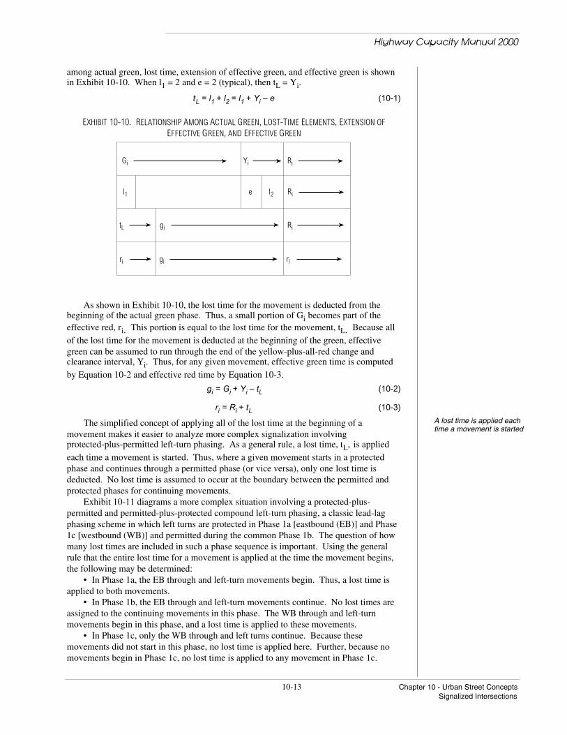
among actual green, lost time, extension of effective green, and effective green is shownin Exhibit 10-10. When l1 = 2 and e = 2 (typical), then tL = Yi.
tL = l1 + l2 = l1 + Yi – e (10-1)
EXHIBIT 10-10. RELATIONSHIP AMONG ACTUAL GREEN, LOST-TIME ELEMENTS, EXTENSION OFEFFECTIVE GREEN, AND EFFECTIVE GREEN
Gi Yi Ri
l1 e l2 Ri
tL gi Ri
ri gi ri
As shown in Exhibit 10-10, the lost time for the movement is deducted from thebeginning of the actual green phase. Thus, a small portion of Gi becomes part of theeffective red, ri. This portion is equal to the lost time for the movement, tL. Because all
of the lost time for the movement is deducted at the beginning of the green, effectivegreen can be assumed to run through the end of the yellow-plus-all-red change andclearance interval, Yi. Thus, for any given movement, effective green time is computed
by Equation 10-2 and effective red time by Equation 10-3.
gi = Gi + Yi – tL (10-2)
ri = Ri + tL (10-3)
A lost time is applied eachtime a movement is started
The simplified concept of applying all of the lost time at the beginning of amovement makes it easier to analyze more complex signalization involvingprotected-plus-permitted left-turn phasing. As a general rule, a lost time, tL, is applied
each time a movement is started. Thus, where a given movement starts in a protectedphase and continues through a permitted phase (or vice versa), only one lost time isdeducted. No lost time is assumed to occur at the boundary between the permitted andprotected phases for continuing movements.
Exhibit 10-11 diagrams a more complex situation involving a protected-plus-permitted and permitted-plus-protected compound left-turn phasing, a classic lead-lagphasing scheme in which left turns are protected in Phase 1a [eastbound (EB)] and Phase1c [westbound (WB)] and permitted during the common Phase 1b. The question of howmany lost times are included in such a phase sequence is important. Using the generalrule that the entire lost time for a movement is applied at the time the movement begins,the following may be determined:
• In Phase 1a, the EB through and left-turn movements begin. Thus, a lost time isapplied to both movements.
• In Phase 1b, the EB through and left-turn movements continue. No lost times areassigned to the continuing movements in this phase. The WB through and left-turnmovements begin in this phase, and a lost time is applied to these movements.
• In Phase 1c, only the WB through and left turns continue. Because thesemovements did not start in this phase, no lost time is applied here. Further, because nomovements begin in Phase 1c, no lost time is applied to any movement in Phase 1c.

Highway Capacity Manual 2000
Chapter 10 - Urban Street Concepts 10-14Signalized Intersections
• In Phase 2, northbound (NB) and southbound (SB) movements begin, and a losttime is applied.
EXHIBIT 10-11. LOST TIME APPLICATION FOR COMPOUND LEFT-TURN PHASING
Indicates lost time applied
Phase 1a Phase 1b Phase 1c Phase 2
Total lost time is the sumof lost time for the paththrough the criticalmovements
The total lost time in the signal cycle, L, is also important. This is the total lost timeinvolved in the critical path through the signal cycle. Determining the critical path andfinding L are discussed in Chapter 16.
TRAFFIC SIGNAL CHARACTERISTICS
Modern traffic signals allocate time in a variety of ways, from the simplesttwo-phase pretimed mode to the most complex multiphase actuated mode.
There are three types of traffic signal controllers:• Pretimed, in which a sequence of phases is displayed in repetitive order. Each
phase has a fixed green time and change and clearance interval that are repeated in eachcycle to produce a constant cycle length.
• Fully actuated, in which the timing on all of the approaches to an intersection isinfluenced by vehicle detectors. Each phase is subject to a minimum and maximumgreen time, and some phases may be skipped if no demand is detected. The cycle lengthfor fully actuated control varies from cycle to cycle.
• Semiactuated, in which some approaches (typically on the minor street) havedetectors and some of the approaches (typically on the major street) have no detectors.
While these equipment-based definitions have persisted in traffic engineeringterminology, the evolution of traffic control technology has complicated their functionfrom the analyst's perspective. For purposes of capacity and level-of-service analysis, itis no longer sufficient to use the controller type as a global descriptor of the intersectionoperation. Instead, an expanded set of these definitions must be applied individually toeach lane group.
Each traffic movement may be served by a phase that is either actuated ornonactuated. Signal phases may be coordinated with neighboring signals on the sameroute, or they may function in an isolated mode without influence from other signals.Nonactuated phases generally operate with fixed minimum green times, which may beextended by reassigning unused green time from actuated phases with low demand, ifsuch phases exist.
Actuated phases are subject to being shortened on cycles with low demand. Oncycles with no demand, they may be skipped entirely, or they may be displayed for theirminimum duration. With systems in which the nonactuated phases are coordinated, theactuated phases are also subject to early termination (force off) to accommodate theprogression design for the system.
Not only the allocation of green time but also the manner in which turningmovements are accommodated within the phase sequence significantly affects capacityand operations at a signalized intersection. Signal phasing can provide for protected,permitted, or not opposed turning movements.

Highway Capacity Manual 2000
10-15 Chapter 10 - Urban Street ConceptsSignalized Intersections
Permitted turning movement
Protected turning movement
A permitted turning movement is made through a conflicting pedestrian or bicycleflow or opposing vehicle flow. Thus, a left-turn movement concurrent with the opposingthrough movement is considered to be permitted, as is a right-turn movement concurrentwith pedestrian crossings in a conflicting crosswalk. Protected turns are those madewithout these conflicts, such as turns made during an exclusive left-turn phase or aright-turn phase during which conflicting pedestrian movements are prohibited.Permitted turns experience the friction of selecting and passing through gaps in aconflicting vehicle or pedestrian flow. Thus, a single permitted turn often consumesmore of the available green time than a single protected turn. Either permitted orprotected turning phases may be more efficient in a given situation, depending on theturning and opposing volumes, intersection geometry, and other factors.
Turning movements that are not opposed do not receive a dedicated left-turn phase(i.e., a green arrow), but because of the nature of the intersection, they are never inconflict with through traffic. This condition occurs on one-way streets, at T-intersections,and with signal phasing plans that provide complete separation between all movements inopposite directions (i.e., split-phase operation). Such movements must be treateddifferently in some cases because they can be accommodated in shared lanes withoutimpeding the through traffic. Left turns that are not opposed at any time should bedistinguished from those that may be unopposed during part of the signal cycle andopposed during another part. Left turns that are opposed during any part of the sequencewill impede through traffic in shared lanes.
SATURATION FLOW RATE
Saturation flow rate is a basic parameter used to derive capacity. It is defined inExhibits 10-8 and 10-9. It is essentially determined on the basis of the minimumheadway that the lane group can sustain across the stop line as the vehicles depart theintersection. Saturation flow rate is computed for each of the lane groups established forthe analysis. A saturation flow rate for prevailing conditions can be determined directlyfrom field measurement and can be used as the rate for the site without adjustment. If adefault value is selected for base saturation flow rate, it must be adjusted for a variety offactors that reflect geometric, traffic, and environmental conditions specific to the siteunder study.
SIGNALIZED INTERSECTION CAPACITYLane group capacity definedCapacity at intersections is defined for each lane group. The lane group capacity is
the maximum hourly rate at which vehicles can reasonably be expected to pass throughthe intersection under prevailing traffic, roadway, and signalization conditions. The flowrate is generally measured or projected for a 15-min period, and capacity is stated invehicles per hour (veh/h).
Traffic conditions include volumes on each approach, the distribution of vehicles bymovement (left, through, and right), the vehicle type distribution within each movement,the location and use of bus stops within the intersection area, pedestrian crossing flows,and parking movements on approaches to the intersection. Roadway conditions includethe basic geometrics of the intersection, including the number and width of lanes, grades,and lane use allocations (including parking lanes). Signalization conditions include a fulldefinition of the signal phasing, timing, and type of control, and an evaluation of signalprogression for each lane group. The analysis of capacity at signalized intersections(Chapter 16) focuses on the computation of saturation flow rates, capacities, v/c ratios,and level of service for lane groups.
LEVEL OF SERVICEControl delay is the servicemeasure that defines LOS
Level of service for signalized intersections is defined in terms of control delay,which is a measure of driver discomfort, frustration, fuel consumption, and increasedtravel time. The delay experienced by a motorist is made up of a number of factors that
Highway Capacity Manual 2000
Chapter 10 - Urban Street Concepts 10-16Signalized Intersections
relate to control, geometrics, traffic, and incidents. Total delay is the difference betweenthe travel time actually experienced and the reference travel time that would result duringbase conditions: in the absence of traffic control, geometric delay, any incidents, and anyother vehicles. Specifically, LOS criteria for traffic signals are stated in terms of theaverage control delay per vehicle, typically for a 15-min analysis period. Delay is acomplex measure and depends on a number of variables, including the quality ofprogression, the cycle length, the green ratio, and the v/c ratio for the lane group.
The critical v/c ratio is an approximate indicator of the overall sufficiency of anintersection. The critical v/c ratio depends on the conflicting critical lane flow rates andthe signal phasing. The computation of the critical v/c ratio is described in detail inAppendix A and in Chapter 16.
Back of queue defined The average back of queue is another performance measure that is used to analyze asignalized intersection. The back of queue is the number of vehicles that are queueddepending on arrival patterns of vehicles and vehicles that do not clear the intersectionduring a given green phase. The computation of average back of queue is explained inAppendix G of Chapter 16.
Levels of service are defined to represent reasonable ranges in control delay.LOS A describes operations with low control delay, up to 10 s/veh. This LOS occurs
when progression is extremely favorable and most vehicles arrive during the green phase.Many vehicles do not stop at all. Short cycle lengths may tend to contribute to low delayvalues.
LOS B describes operations with control delay greater than 10 and up to 20 s/veh.This level generally occurs with good progression, short cycle lengths, or both. Morevehicles stop than with LOS A, causing higher levels of delay.
Cycle failure occurswhen a given greenphase does not servequeued vehicles, andoverflows occur
LOS C describes operations with control delay greater than 20 and up to 35 s/veh.These higher delays may result from only fair progression, longer cycle lengths, or both.Individual cycle failures may begin to appear at this level. Cycle failure occurs when agiven green phase does not serve queued vehicles, and overflows occur. The number ofvehicles stopping is significant at this level, though many still pass through theintersection without stopping.
LOS D describes operations with control delay greater than 35 and up to 55 s/veh.At LOS D, the influence of congestion becomes more noticeable. Longer delays mayresult from some combination of unfavorable progression, long cycle lengths, and highv/c ratios. Many vehicles stop, and the proportion of vehicles not stopping declines.Individual cycle failures are noticeable.
LOS E describes operations with control delay greater than 55 and up to 80 s/veh.These high delay values generally indicate poor progression, long cycle lengths, and highv/c ratios. Individual cycle failures are frequent.
LOS F describes operations with control delay in excess of 80 s/veh. This level,considered unacceptable to most drivers, often occurs with oversaturation, that is, whenarrival flow rates exceed the capacity of lane groups. It may also occur at high v/c ratioswith many individual cycle failures. Poor progression and long cycle lengths may alsocontribute significantly to high delay levels.
Delays in the range of LOS F (unacceptable) can occur while the v/c ratio is below1.0. Very high delays can occur at such v/c ratios when some combination of thefollowing conditions exists: the cycle length is long, the lane group in question isdisadvantaged by the signal timing (has a long red time), and the signal progression forthe subject movements is poor. The reverse is also possible (for a limited duration): asaturated lane group (i.e., v/c ratio greater than 1.0) may have low delays if the cyclelength is short or the signal progression is favorable, or both.
Thus, the designation LOS F does not automatically imply that the intersection,approach, or lane group is over capacity, nor does an LOS better than E automaticallyimply that unused capacity is available.
Highway Capacity Manual 2000
10-17 Chapter 10 - Urban Street ConceptsSignalized Intersections
The method in this chapter and Chapter 16 requires the analysis of both capacity andLOS conditions to fully evaluate the operation of a signalized intersection.
REQUIRED INPUT DATA AND ESTIMATED VALUES
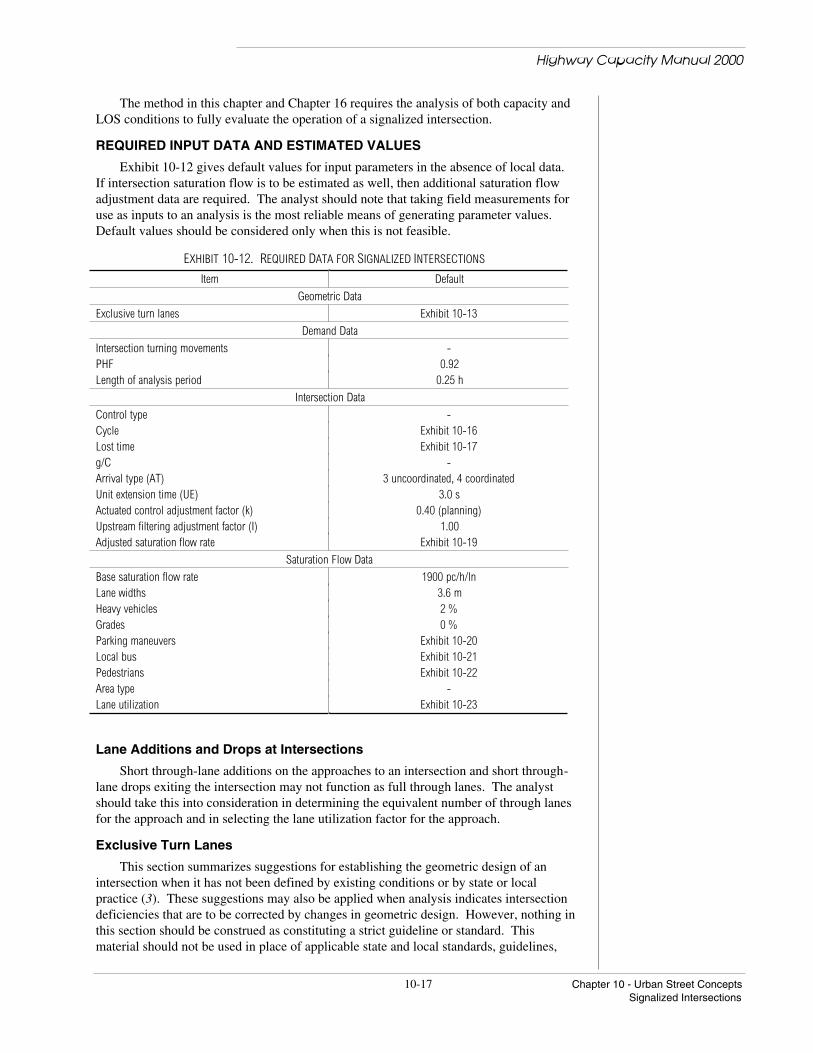
Exhibit 10-12 gives default values for input parameters in the absence of local data.If intersection saturation flow is to be estimated as well, then additional saturation flowadjustment data are required. The analyst should note that taking field measurements foruse as inputs to an analysis is the most reliable means of generating parameter values.Default values should be considered only when this is not feasible.
EXHIBIT 10-12. REQUIRED DATA FOR SIGNALIZED INTERSECTIONS
Item Default
Geometric Data
Exclusive turn lanes Exhibit 10-13
Demand Data
Intersection turning movements -PHF 0.92Length of analysis period 0.25 h
Intersection Data
Control type -Cycle Exhibit 10-16Lost time Exhibit 10-17g/C -Arrival type (AT) 3 uncoordinated, 4 coordinatedUnit extension time (UE) 3.0 sActuated control adjustment factor (k) 0.40 (planning)Upstream filtering adjustment factor (I) 1.00Adjusted saturation flow rate Exhibit 10-19
Saturation Flow Data
Base saturation flow rate 1900 pc/h/lnLane widths 3.6 mHeavy vehicles 2 %Grades 0 %Parking maneuvers Exhibit 10-20Local bus Exhibit 10-21Pedestrians Exhibit 10-22Area type -Lane utilization Exhibit 10-23
Lane Additions and Drops at Intersections
Short through-lane additions on the approaches to an intersection and short through-lane drops exiting the intersection may not function as full through lanes. The analystshould take this into consideration in determining the equivalent number of through lanesfor the approach and in selecting the lane utilization factor for the approach.
Exclusive Turn Lanes
This section summarizes suggestions for establishing the geometric design of anintersection when it has not been defined by existing conditions or by state or localpractice (3). These suggestions may also be applied when analysis indicates intersectiondeficiencies that are to be corrected by changes in geometric design. However, nothing inthis section should be construed as constituting a strict guideline or standard. Thismaterial should not be used in place of applicable state and local standards, guidelines,

Highway Capacity Manual 2000
Chapter 10 - Urban Street Concepts 10-18Signalized Intersections
policies, or practice. Rather it is presented here to indicate general possibilities forimprovement of signalized intersections.
Exclusive Left-Turn Lanes
The presence of exclusive left-turn lanes is determined by the volume of left-turntraffic, opposing volumes, and safety considerations (4). For analyses of futureconditions requiring assumptions about lane configurations, Exhibit 10-13 showsrelationships between left-turn volumes and the probable need for left-turn lanes in theabsence of local data (5).
EXHIBIT 10-13. TURN VOLUMES PROBABLY REQUIRING EXCLUSIVE LEFT-TURN LANES AT SIGNALIZEDINTERSECTIONS
Turn Lane Minimum Turn Volume (veh/h)
Single exclusive left-turn lane 100Double exclusive left-turn lanes 300
Exclusive left-turn lanes are also required when an exclusive left-turn phase iswarranted at a signalized intersection. In the absence of forecast turn volumes, theanalyst should assume that exclusive left-turn lanes will be the standard design for allfuture intersections, except possibly in the central business district (CBD) (if severe right-of-way constraints exist), on a one-way street, or where the operating jurisdiction doesnot typically construct such lanes.
Exclusive Right-Turn Lanes
Although right turns are generally made more efficiently than left turns, exclusiveright-turn lanes are often provided for many of the same reasons that left-turn lanes areused. Right turns may face a conflicting pedestrian or bicycle flow, but they do not face aconflicting vehicular flow. In general, an exclusive right-turn lane should be consideredif the right-turn volume exceeds 300 veh/h and the adjacent mainline volume exceeds 300veh/h/ln.
Number of Lanes
The number of lanes required on an approach depends on a variety of factors,including the signal design. In general, enough main roadway lanes should be providedto prevent the total of the through plus right-turn volume (plus left-turn volume, ifpresent) from exceeding 450 veh/h/ln. This is a very general suggestion. Higher volumescan be accommodated on major approaches if a substantial portion of available greentime can be allocated to the subject approach. If the number of lanes is unknown, theforegoing value is a reasonable starting point for analysis.
Other Features
If lane widths are unknown, the 3.6-m standard lane width should be assumed unlessknown restrictions prevent such width. Parking conditions consistent with local practiceshould be assumed. If no information exists, no curb parking and no local buses shouldbe assumed for analysis purposes.
The storage bay length of exclusive turn lanes should be sufficient to handle theturning traffic without reducing the safety or capacity of the approach. A method forestimating the required length of the storage bay is presented in Appendix G of Chapter16.
Highway Capacity Manual 2000
10-19 Chapter 10 - Urban Street ConceptsSignalized Intersections
Intersection Turning Movements
Intersection turning movements are used in the analysis of signalized intersections onurban streets. If signal timing is not known, then the turning movements may also beused to estimate the effective green ratios (g/C) and cycle length for each intersection.
Default Values in Absence of Turning Movement DataSee Chapter 9 for means ofestimating peak demandsfrom ADT
An urban street analysis can be performed in the absence of intersection turningmovement data if the analyst can obtain directional volume counts for the urban streetand estimate the average percentage of turning vehicles on the street approaches at theintersections. Peak-hour volumes by direction can be estimated from average daily traffic(ADT). The estimated percentage of turns is used to reduce the total urban streetapproach volume at intersections where exclusive turn lanes are provided. Thepercentage of turns made from exclusive lanes at an intersection is subject to localconditions. In the complete absence of local information, default values of 10 percent torepresent right turns and 10 percent for left turns as a percentage of the total approachtraffic are suggested.
If some of the intersections have exclusive lanes and some do not, the delay at eachintersection along the urban street should be computed and summed to obtain theintersection delay for the section. If this is not feasible, the analyst can divide theintersections into two categories: intersections with exclusive lanes and intersectionswithout exclusive lanes. The delay can be computed for each category of intersection,multiplied by the number of intersections in that category, and summed to obtainintersection delay on the urban street.
Turning Movement Estimation
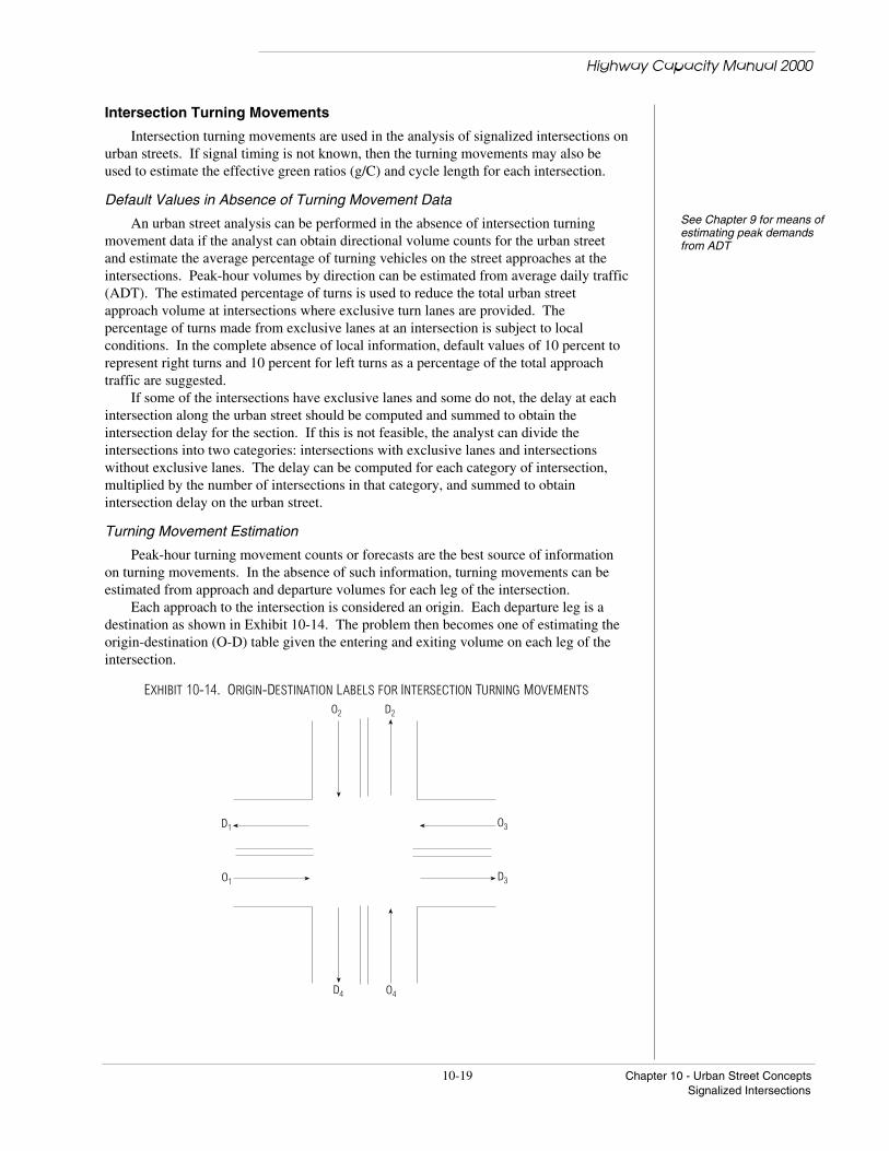
Peak-hour turning movement counts or forecasts are the best source of informationon turning movements. In the absence of such information, turning movements can beestimated from approach and departure volumes for each leg of the intersection.
Each approach to the intersection is considered an origin. Each departure leg is adestination as shown in Exhibit 10-14. The problem then becomes one of estimating theorigin-destination (O-D) table given the entering and exiting volume on each leg of theintersection.
EXHIBIT 10-14. ORIGIN-DESTINATION LABELS FOR INTERSECTION TURNING MOVEMENTSO2 D2
O3
D3
O4D4
O1
D1

Highway Capacity Manual 2000
Chapter 10 - Urban Street Concepts 10-20Signalized Intersections
This estimation procedure is derived from research (6). The procedure assumes thatthe number of vehicles going from one leg to another is directly proportional to the totalvolume entering the one leg and the total volume exiting on the other leg. Thisassumption may not be valid when other factors or geometric situations are present, suchas a nearby freeway on-ramp, which may attract a much higher than normal trip volume.Equation 10-4 is used to estimate the turning movement O-D matrix:
T ij =T i *T j
T iji∑
(10-4)
whereTij = number of trips going from origin leg i to destination leg j,Ti = number of trips originating at origin i, andTj = number of trips leaving at destination j.
U-turns (Ti = j) trips are assigned a value of zero unless the analyst is aware of a
reason for U-turns to be a significant number. Note that Equation 10-4 does not ensurethat the final estimates of total trips exiting each leg of the intersection will match theinitial value. An iterative procedure can be used to increase or reduce the Tij as necessaryto ensure that the sum of the Tij is close to the initial demand estimates for each entering
and departing leg of the intersection. This procedure is known as a matrix balancingprocess (7).
The steps of the iterative procedure use Equations 10-5, 10-6, 10-7, and 10-8.Step 1. Compute the ratio of desired to actual exiting volume for each departure leg.
R j =T j
T iji∑
(10-5)
whereRj = ratio of desired to actual exiting volume for exit leg j,Tj = desired exiting volume for exit leg j, andTij = current estimate of volume going from origin i to destination j.
Step 2. Multiply all Tij for that exit leg by ratio Rj. Repeat for each exit leg.
Step 3. Compute ratio of desired to actual entering volumes for each entering leg i.
Ri = T i
T ijj
∑(10-6)
whereRi = ratio of desired to actual entering volume for entry leg i,Ti = desired entering volume for entry leg i, andTij = current estimate of volume going from origin i to destination j.
Step 4. Multiply all Tij for that entry leg by ratio Ri. Repeat for each entry leg.
Step 5. Determine whether the user-specified number of iterations has beenexhausted or the user-specified closure criterion is met for all entry and exit legs.
diff i = T i − T ijj
∑ for entry legs (10-7)
diff j = T j − T iji∑ for exit legs (10-8)
Step 6. If any of the computed differences is greater than the closure criterion (aclosure criterion of 10 veh/h is suggested) and the iteration limit has not been exceeded,then go back to Step 1.
Highway Capacity Manual 2000
10-21 Chapter 10 - Urban Street ConceptsSignalized Intersections
Peak-Hour Factor
Refer to the peak-hour factor discussion in this chapter under Section II, UrbanStreets, Required Input Data and Estimated Values.
Length of Analysis Period
Refer to the length of analysis period discussion in this chapter under Section II,Urban Streets, Required Input Data and Estimated Values.
Intersection Control Type
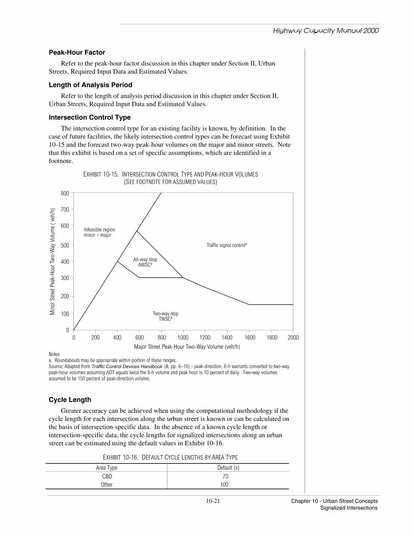
The intersection control type for an existing facility is known, by definition. In thecase of future facilities, the likely intersection control types can be forecast using Exhibit10-15 and the forecast two-way peak-hour volumes on the major and minor streets. Notethat this exhibit is based on a set of specific assumptions, which are identified in afootnote.
EXHIBIT 10-15. INTERSECTION CONTROL TYPE AND PEAK-HOUR VOLUMES(SEE FOOTNOTE FOR ASSUMED VALUES)
0 200 400 600 800 1000 1200 1400 1600 1800 2000
800
700
600
500
400
300
200
100
0
Major Street Peak-Hour Two-Way Volume (veh/h)
Min
or S
treet
Pea
k-Ho
ur T
wo-
Way
Vol
ume
( veh
/h)
Infeasible regionminor > major
Traffic signal controla
All-way stopAWSCa
Two-way stopTWSCa
Notesa. Roundabouts may be appropriate within portion of these ranges.Source: Adapted from Traffic Control Devices Handbook (8, pp. 4–18) - peak-direction, 8-h warrants converted to two-waypeak-hour volumes assuming ADT equals twice the 8-h volume and peak hour is 10 percent of daily. Two-way volumesassumed to be 150 percent of peak-direction volume.
Cycle Length
Greater accuracy can be achieved when using the computational methodology if thecycle length for each intersection along the urban street is known or can be calculated onthe basis of intersection-specific data. In the absence of a known cycle length orintersection-specific data, the cycle lengths for signalized intersections along an urbanstreet can be estimated using the default values in Exhibit 10-16.
EXHIBIT 10-16. DEFAULT CYCLE LENGTHS BY AREA TYPE
Area Type Default (s)
CBD 70Other 100

Highway Capacity Manual 2000
Chapter 10 - Urban Street Concepts 10-22Signalized Intersections
If the results of the urban street or intersection analysis indicate that the criticalvolume/capacity ratios for one or more intersections will be greater than 1.00, then theanalyst should perform an overall review of geometrics, signal timing, and signal phasingand should consider increasing the cycle length until the v/c ≤ 1.00. Special analysisprocedures for actuated signals are given in Appendix B of Chapter 16. A simplerapproach is also presented in Appendix A of this chapter.
Lost Time and Estimation of Signal Phasing
The total lost time in the signal cycle can be obtained from Exhibit 10-17 on thebasis of whether left turns are protected or permitted for the major street and the minorstreet.
EXHIBIT 10-17. DEFAULT LOST TIME PER CYCLE BY LEFT PHASE TYPE
Major Street Minor Street Number of Phases L (s)
Protected Protected 4 16Protected Permitted 3 12Permitted Protected 3 12Permitted Permitted 2 8
Note:Protected and permitted refer to left turns.
Unopposed left turns (left turns made from a one-way street or from the unopposedleg of a T-intersection) are treated as permitted, while protected-plus-permitted left turnscan be treated as protected when using Exhibit 10-17. Exhibit 10-17 shows that 4 s oflost time occurs between phases of the signal. Note that the term “phase” is used here asit is defined in this manual and should not be confused with the term “NEMA phase,”which is used in traffic-actuated control to refer to the green time for a single movement.Thus, an eight-phase NEMA controller (which has protected left turns for all fourapproaches) has four phases.
The actual left-turn treatment should be used, if known, in determining the lost time.If this is unknown, the choice should be made using local policies or practices. Manyagencies use the product of the left-turn and opposing through traffic volumes as anindicator of the need for protected phasing. The following criteria and thresholds may beused to determine whether a left turn is likely to need a protected left-turn phase.
Criteria for considerationof providing a protectedleft-turn phase
Left turns should be considered for protected phases if any of the following criteria ismet:
• More than one turning lane is provided,• The left turn has a demand in excess of 240 veh/h over 1 h, or• The cross product of left-turn demand and the opposing through demand for 1 h
exceeds 50,000 for one opposing through lane, 90,000 for two opposing through lanes, or110,000 for three or more opposing through lanes.
Note that these thresholds should only be used for planning applications. For designand operational purposes many other factors should be considered, including accidentexperience, field observations, and conditions that may exist outside of the analysisperiod. The Traffic Control Devices Handbook (8, pp. 4–18) has more information onleft-turn phase warrants.
Unprotected left turns from exclusive lanes receive no explicit assignment of greentime because they are assumed to be accommodated by green time for the concurrentthrough movement.
Split phase operation provides complete separation between movements in opposingdirections by allowing all movements from only one approach to proceed at the sametime. This alternative can be assumed for planning purposes only if
• A pair of opposing approaches is physically offset by more than 20 m,

Highway Capacity Manual 2000
10-23 Chapter 10 - Urban Street ConceptsSignalized Intersections
• A protected left-turn phase must be provided to two opposing single-laneapproaches, or
• Both opposing left turns are protected and one of the left turns is accommodatedwith an exclusive lane plus an optional lane for through and left-turning traffic.
Effective Green Ratio
It is best to use the actual effective green time ratio (g/C) for each movement. In thecase of semiactuated and fully actuated signals, the g/C ratios are measured in the fieldand averaged over several signal cycles during the analysis period. The next best methodis to estimate the g/C ratio from intersection turning movements, as described inAppendix A and Appendix B of Chapter 16.
Weighted g/C for urban streetA through g/C for each intersection is desirable; however, for planning purposes, aweighted g/C may be appropriate. The weighted g/C of an urban street is the average ofthe critical intersection through g/C and the average of all the other g/C's for the urbanstreet. For example, if there are four signals with a through g/C of 0.50 and one signalwith a through g/C of 0.40, the weighted average g/C for the urban street is 0.45. Theweighted g/C takes into account the adverse effect of the critical intersection and theoverall quality of flow for the urban street. An overall default of 0.45 may be used for themajor street through movement, but it should be recognized that appropriate ratios canvary depending on characteristics of the urban street.
Arrival Type
The quality of progression is used to determine the arrival type as shown in Exhibit10-18. The arrival type is used to adjust the computed delay for traffic at each signal. Ifthe arrival type is unknown, a default value of 3 is used for uncoordinated movementsand a default value of 4 is used for coordinated movements. Exhibit 15-4 provides amore precise means of determining the arrival type when the proportion of vehiclesarriving on green is known.
EXHIBIT 10-18. PROGRESSION QUALITY AND ARRIVAL TYPE
ProgressionQuality
ArrivalType
Conditions Under Which Arrival Type Is Likely To Occur
Very poor 1 Occurs for coordinated operation on two-way street where one direction of traveldoes not receive good progression. Signals are spaced less than 500 m apart.
Unfavorable 2 A less extreme version of Arrival Type 1. Signals spaced at or more than 500 mbut less than 1000 m apart.
Random arrivals 3 Isolated signals spaced at or more than 1000 m apart (whether or notcoordinated).
Favorable 4 Occurs for coordinated operation, often only in one direction on a two-way street.Signals are typically between 500 m and 1000 m apart.
Highly favorable 5 Occurs for coordinated operation. More likely to occur with signals less than 500m apart.
Exceptional 6 Typical of one-way streets in dense networks and central business districts.Signal spacing is typically under 250 m.
Progression Adjustment Factor
Exhibit 16-12 in Chapter 16 provides guidance on selecting the progressionadjustment factor (PF) on the basis of arrival type. The PF = 1.00 for Arrival Type 3.The PF for Arrival Type 4 is 0.84, when g/C is equal to 0.45.

Chapter 10 - Urban Street Concepts 10-24Signalized Intersections
Incremental Delay Adjustment
The incremental delay adjustment (or actuated control adjustment factor), k, is set to0.50 for pretimed signal control. The same value is used for the nonactuated movementsat an intersection with actuated control or semiactuated control.
For the actuated movements, the factor can vary from 0.04 to 0.50, depending on theunit extension for each vehicle actuation and the volume/capacity ratio (X) for themovement. The value of the adjustment factor increases as the volume/capacity ratioincreases. Exhibit 15-6 provides guidance on the selection of k given the unit extensionand the degree of saturation. In the absence of this information, the analyst may use avalue of 0.40 for k, which corresponds to a unit extension of 3 s and a volume/capacityratio between 0.85 and 0.90. For operational analyses in Chapter 16, the value of kshould be based on the computed v/c ratio.
Upstream Filtering/Metering Adjustment Factor
The incremental delay adjustment term (I) accounts for the effects of upstreamsignals metering arrivals at the study intersection. If the nearest upstream signal is 1.0km or more away from the subject movement at the study intersection, then I is set to 1.0.Otherwise, I varies from 0.92 to 0.09, decreasing with increasing degree of saturation forthe upstream signal. In the absence of this information, the analyst may use a value of1.0, which applies to isolated intersections, for I.
Base Saturation Flow RateThe default basesaturation flow rate is1,900 pc/h/ln
This manual uses a default base saturation flow rate of 1,900 pc/h/ln. This value maybe increased or decreased on the basis of local field measurements. Approaches withlower approach speeds (less than 50 km/h) often have lower base saturation flow rates, onthe order of 1,800 pc/h/ln. Approaches with higher approach speeds (greater than 80km/h) may have base saturation flow rates higher than 1,900 pc/h/ln.
Adjusted Saturation Flow Rates
The adjusted saturation flow rate per lane is used to compute the delay to throughmovements at each intersection due to signal control. Initial estimates of the adjustedsaturation flow rate for through lanes can be obtained from Exhibit 10-19.
EXHIBIT 10-19. ADJUSTED SATURATION FLOW RATE BY AREA TYPE
Area Type Default Value (veh/h/ln) Range (veh/h/ln)
CBD 1700 1600–1800Other 1800 1700–1950
These adjusted saturation flow rates can also be used for intersection analyses.However, if local data are available on the specific geometry and demand conditions oneach approach of an intersection, then the adjusted saturation flow rates can be estimatedmore accurately. Chapter 16 provides a more accurate method for computing adjustedsaturation flow rates when additional data are available.
Lane Widths
The typical lane width is 3.6 m. Urban street lane widths can be as narrow as 3.0 m.The lane closest to a raised median may be extra wide to allow for some shy distancebetween vehicles and the median. The rightmost lane may be several meters wider thanthe standard. Lanes wider than 6.0 m should be evaluated to determine whether driversuse the lane as two lanes or as a single wide lane. Drivers making right turns from a widethrough lane next to the curb may often form a second queue next to the through vehicles.In this case, the wide through lanes might be analyzed as two lanes: a standard-widththrough lane plus a narrow exclusive right-turn lane.
Highway Capacity Manual 2000

Highway Capacity Manual 2000
10-25 Chapter 10 - Urban Street ConceptsSignalized Intersections
The lane width used for the analysis excludes parking lanes (occupied by parkedvehicles). Bicycle lanes that are striped to allow right-turning vehicles to enter them forthe last several meters before the intersection may be included in the overall lane width ofthe curb lane.
Heavy Vehicles
The local highway performance management system can be used to obtain localinformation on the percentage of heavy vehicles by facility and area type. Thebreakdown between recreational vehicles, trucks, and buses is not used in thecomputation of adjusted saturation flow rates at signalized intersections. In the absenceof local data, a default value of 2 percent heavy vehicles (including all types) may beused for urban streets.
Grades
The approach grade becomes important only when it is significantly steeper than 4percent. The maximum grades encountered on urban streets typically range from 6 to 11percent but can reach 31 percent in extreme situations, such as in San Francisco,California. The analyst, in the absence of specific local data, may use 0 percent foressentially flat approaches, 3 percent for moderate grades, and 6 percent for relativelysteep grades.
Parking Maneuvers
The number of parking maneuvers per hour is best measured in the field. In theabsence of such data, it can be estimated from the number of parking spaces within 80 mof the stop line and the average turnover rate for each space. The number of spaceswithin 80 m of the stop line is estimated assuming 8 m per space. Each turnover (one carleaving and one car arriving) generates two parking maneuvers. Exhibit 10-20 givesdefault values for maneuvers per hour, based on 80 percent occupancy of the spaces.These default values may be used in the absence of local data.
EXHIBIT 10-20. PARKING MANEUVER DEFAULTS
Street Type Number of Spaces in 80 m Parking Time Limit (h) Turnover Rateper Hour
Maneuversper Hour
Two-way 10 1 1 162 0.5 8
One-way 20 1 1 322 0.5 16
Note:Assumed parking space occupancy of 80 percent.
Local Buses
The number of buses per hour stopping at bus stops within 80 m of the stop line canbe estimated from bus schedules for existing conditions. In the absence of such data, thedefault values in Exhibit 10-21 may be used for intersections where buses are expected tostop.
EXHIBIT 10-21. BUS FREQUENCY DEFAULTS
Area Type Average Bus Headway (min) Buses Stopping/h
CBD 5 12Other 30 2

Highway Capacity Manual 2000
Chapter 10 - Urban Street Concepts 10-26Signalized Intersections
Pedestrians
Field counts are the best source of information on pedestrian flows. In the absenceof counts the defaults listed in Exhibit 10-22 may be used. The analyst should recognizethe tendency of field observers to underestimate pedestrian flows when casuallyobserving intersection operations. Relatively infrequent appearances of pedestrians at theintersection, such as one pedestrian per cycle or one pedestrian per minute, can add up tofairly significant hourly pedestrian flows of 60 p/h.
EXHIBIT 10-22. DEFAULTS FOR PEDESTRIAN FLOWS
Area Type Pedestrian Volume (p/h)
CBD 400Other 50
Area Type
Only two area types are recognized for signalized intersection analysis: CBD andother. The base saturation flow rate for an intersection is reduced 10 percent for CBDconditions compared with other areas. This adjustment is in addition to the saturationflow reductions for the higher number of parking maneuvers, pedestrians, and bus stopstypical of CBDs.
Lane Utilization
The assumed lane utilization can be based on default values unless field data areavailable or the analyst is aware of special conditions (such as short lane drops or adownstream freeway on-ramp) that might cause drivers to distribute themselves unevenlyacross the available lanes on the approach. As demand approaches capacity, the analystmay use lane utilization factors closer to 1.0, which would indicate a more uniform use ofthe available lanes and less opportunity for drivers to freely select their lane. Exhibit10-23 summarizes lane utilization adjustment factors for different lane group movementsand numbers of lanes.
EXHIBIT 10-23. DEFAULT LANE UTILIZATION ADJUSTMENT FACTORS
Lane Group Movements No. of Lanes in LaneGroup
Traffic in Most HeavilyTraveled Lane (%)
Lane UtilizationAdjustment Factor (fLU)
Through or shared 1 100.0 1.0002 52.5 0.9523a 36.7 0.908
Exclusive left turn 1 100.0 1.0002a 51.5 0.971
Exclusive right turn 1 100.0 1.0002a 56.5 0.885
Note:a. If lane group has more lanes than shown in this exhibit, it is recommended that surveys be made or the smallest fLU shownfor that type of lane group be used.
SERVICE VOLUME TABLE
Exhibit 10-24 shows the example service volumes (veh/h) that can be accommodatedby a given LOS and number of through lanes to provide the desired LOS on an approach(assuming that all other approaches have the same hourly volume). The values are basedon assumptions given in a footnote to the exhibit.

Highway Capacity Manual 2000
10-27 Chapter 10 - Urban Street ConceptsSignalized Intersections
EXHIBIT 10-24. EXAMPLE SERVICE VOLUMES FOR SIGNALIZED INTERSECTION(SEE FOOTNOTE FOR ASSUMED VALUES)
LOS
Through Lanes A B C D E
Service Volumes (veh/h)
1 N/A 130 350 530 5902 N/A 200 860 1090 12203 N/A N/A 1230 1510 1680
NotesN/A - not achievable given assumptions listed below.This table is derived from the following assumptions.a. Entries are total hourly volumes for subject approach including turns.b. All approaches of intersection have the same demand as the subject approach.c. Left turns equal to 10% of approach demand. Right turns equal to 10% of approach demand.d. Phasing is protected lefts with exclusive left-turn lane in addition to through lanes.e. All approaches are two-way streets.f. Peak-hour factor = 0.92.g. Saturation flow for each approach is computed assuming the following defaults: lane width = 3.6 m, percent heavy vehicles =2%, grades = 0%, parking = 8/h, bus = 2/h, pedestrians = 50/h, area type = CBD, lane utilization = 1.05 for 2 lane, 1.10 for 3lanes, base saturation flow rate = 1900 pc/h/ln. These assumptions result in adjusted saturation flow rates of 1770 for the left-turn lanes and 1560 veh/h/ln for the through lanes.h. Lost time is 16 s.i. No upstream signal (I = 1.0).j. Pretimed signal (k = 0.50).k. Arrival type = 3.l. Analysis period (T) = 0.25 h.m. Initial queue = 0.n. Signal timing set to maximize service volumes subject to pedestrian clearance time requirements, minimum phase lengths,and maximum signal length of 150 s.o. Cycle lengths are as follows.
Through Lanes LOS A LOS B LOS C LOS D LOS E1 N/A 60 s 60 s 110 s 150 s2 N/A 70 s 80 s 110 s 150 s3 N/A N/A 80 s 100 s 150 s
Note that minimum cycle lengths to serve pedestrians are 60 s for single-lane approach intersection, 70 s for two-lane approachintersection, and 80 s for a three-lane approach intersection. Minimum pedestrian clearance times are 3 s per through lane plus3 s for left-turn lane plus 6 s walk display. Minimum left-turn phase was set at 6 s plus phase change and clearance interval of4 s.
IV. UNSIGNALIZED INTERSECTIONS
Three types of unsignalized intersections are addressed in this manual: two-way stop-controlled (TWSC), all-way stop-controlled (AWSC), and roundabouts.
CHARACTERISTICS OF TWSC INTERSECTIONS
TWSC intersections are common in the United States and abroad. Stop signs areused to control vehicle movements at such intersections. At TWSC intersections, thestop-controlled approaches are referred to as the minor street approaches; they can beeither public streets or private driveways. The intersection approaches that are notcontrolled by stop signs are referred to as the major street approaches.
A three-leg intersection is considered to be a standard type of TWSC intersection ifthe single minor street approach (i.e., the stem of the T configuration) is controlled by astop sign. Three-leg intersections where two of the three approaches are controlled bystop signs are a special form of unsignalized intersection control.
FLOW AT TWSC INTERSECTIONS
TWSC intersections assign the right-of-way among conflicting traffic streamsaccording to the following hierarchy:

Highway Capacity Manual 2000
Chapter 10 - Urban Street Concepts 10-28Unsignalized Intersections
STOP
STOP
13
16
15
14
Four-leg intersection
7
Rank Traffic stream1 2, 3, 5, 6, 15, 162 1, 4, 13, 14, 9, 123 8, 114 7, 10
8 9
121110
123
654
Rank 1 All conflicting movements yield the right-of-way to any through orright-turning vehicle on the major street approaches. The major streetthrough and right-turning movements are the highest-priority movementsat a TWSC intersection.
Rank 2 Vehicles turning left from the major street onto the minor street yield onlyto conflicting major street through and right-turning vehicles. All otherconflicting movements at a TWSC intersection yield to these major streetleft-turning movements. Vehicles turning right from the minor street ontothe major street yield only to conflicting major street through movements.
Rank 3 Minor street through vehicles yield to all conflicting major street through,right-turning, and left-turning movements.
Rank 4 Minor street left-turning vehicles yield to all conflicting major streetthrough, right-turning, and left-turning vehicles and to all conflictingminor street through and right-turning vehicles.
Even though the hierarchy described above suggests that the highest-prioritymovements experience no delay as they travel through a TWSC intersection, experienceshows that their right-of-way is sometimes preempted by other conflicting movements.Such preemptions most often occur during periods of congestion when vehicles in theconflicting movements are experiencing long delays and queues (or when separate left-turn bays are not provided on the major street).
GAP ACCEPTANCE MODELS
Gap acceptance models begin with the recognition that TWSC intersections give nopositive indication or control to the driver on the minor street as to when it is safe to leavethe stop line and enter the major traffic stream. The driver must determine both when agap in the major stream is large enough to permit safe entry and when it is the driver'sturn to enter on the basis of the relative priority of the competing traffic streams. Thisdecision-making process has been formalized into what is commonly known as gapacceptance theory. Gap acceptance theory includes three basic elements: the size anddistribution (availability) of gaps in the major traffic stream, the usefulness of these gapsto the minor stream drivers, and the relative priority of the various traffic streams at theintersection.
Availability of Gaps
The first element to consider is the proportion of gaps of a particular size in themajor traffic stream offered to the driver entering from the minor stream, as well as thepattern of arrival times of vehicles. The distribution of gaps between the vehicles in thedifferent streams has a major effect on the performance of the intersection.
Usefulness of GapsCritical gap is theminimum time betweensuccessive major streetvehicles where minorstreet vehicles make amaneuver
Follow-up time is thetime span between thedeparture of one vehiclefrom the minor street andthe departure of the nextvehicle using the samegap
The second element to consider is the extent to which drivers find gaps of aparticular size useful when attempting to enter the intersection. It is generally assumed ingap acceptance theory that drivers are both consistent and homogeneous. In reality, thisassumption is not entirely correct. Studies have demonstrated that different drivers havedifferent gap acceptance thresholds and even that the gap acceptance threshold of anindividual driver often changes over time (9). In this manual the critical gap and follow-up times are considered representative of a statistical average of the driver population inthe United States.
Relative Priority of Various Streams at the Intersection
Different streams have different ranking in a priority hierarchy. The gap acceptanceprocess evaluates them with impedance terms through the order of departures. Typically,gap acceptance processes assume that drivers on the major road or stream are unaffected

Highway Capacity Manual 2000
10-29 Chapter 10 - Urban Street ConceptsUnsignalized Intersections
by the minor stream drivers. If this is not the case, the gap acceptance process has to bemodified.
CAPACITY OF TWSC INTERSECTIONS
At TWSC intersections, drivers on the controlled approaches are required to selectgaps in the major street flow through which to execute crossing or turning maneuvers onthe basis of judgment. In the presence of a queue, each driver on the controlled approachmust also use some time to move into the front-of-queue position and prepare to evaluategaps in the major street flow. Thus, the capacity of the controlled legs is based on threefactors: the distribution of gaps in the major street traffic stream, driver judgment inselecting gaps through which to execute the desired maneuvers, and the follow-up timerequired by each driver in a queue.
The basic capacity model assumes that gaps in the conflicting stream are randomlydistributed. When traffic signals on the major street are within 0.4 km of the subjectintersection, flows may not be random but will likely have some platoon structure.
Pedestrians crossing an intersection impede lower-ranked minor street vehicles, butonly one lane at a time. This is because vehicles performing a given through or turningmovement tend to pass in front of or behind pedestrians once a driver’s target lane isclear. Pedestrian flows are counted somewhat differently than are vehicle flows. If thetypical pattern is for pedestrians to walk individually, each pedestrian is countedindividually in the pedestrian flow. However, if pedestrians tend to cross in groups, thenumber of groups is counted. The important factor is to determine the number ofblockages. In most cases, this will be a combination of individual pedestrians and groupsof pedestrians. Thus, as defined for the purpose of determining the pedestrian impedance,the pedestrian volume is the sum of individual pedestrians crossing individually andgroups of pedestrians crossing together during the analysis time period.
The existence of a raised or striped median or a two-way left-turn lane (TWLTL) onthe major street often causes some degree of a gap acceptance phenomenon known as“two-stage gap acceptance.” For example, the existence of a raised or striped mediancauses a significant proportion of the minor street drivers to first cross part of the majorstreet approach and then pause in the middle of the road to wait for another gap in theother approach. If a TWLTL exists on the major street, the minor street left-turn vehicleusually merges into the TWLTL first, then seeks a usable gap on the other approach whileslowly moving some distance along the TWLTL. Both of these behaviors can increasecapacity.
The geometric elements near the stop line on the stop-controlled approaches of manyintersections may result in a higher capacity than the shared-lane capacity equation maypredict. This is because, at such approaches, two vehicles may occupy or depart from thestop line simultaneously as a result of a large curb radius, a tapered curb, or a parkingprohibition. The magnitude of this effect will depend in part on the turning movementvolumes and the resultant probability of two vehicles being simultaneously at the stopline and on the storage length available to feed the second position at the stop line.
Often, two or three movements share a single lane on the minor approach. With thislane sharing, vehicles from different movements do not have simultaneous access to gaps,nor can more than one vehicle from the sharing movements use the same gap, whichinfluences capacity.
The existence of nearby signalized intersections (i.e., traffic signals on the majorstreet within 0.4 km of the subject intersection) typically causes vehicles to arrive at theintersection in platoons. This influences the size and distribution of available gaps andmay cause an increase in the minor street capacity. The greater the number of vehiclestraveling in platoons, the higher the minor street capacity for a given opposing volume.This is due to the greater proportion of large gaps that more than one minor street vehiclecan use. If signalized intersections exist upstream of the subject intersection in bothdirections, the effect is much more complex.
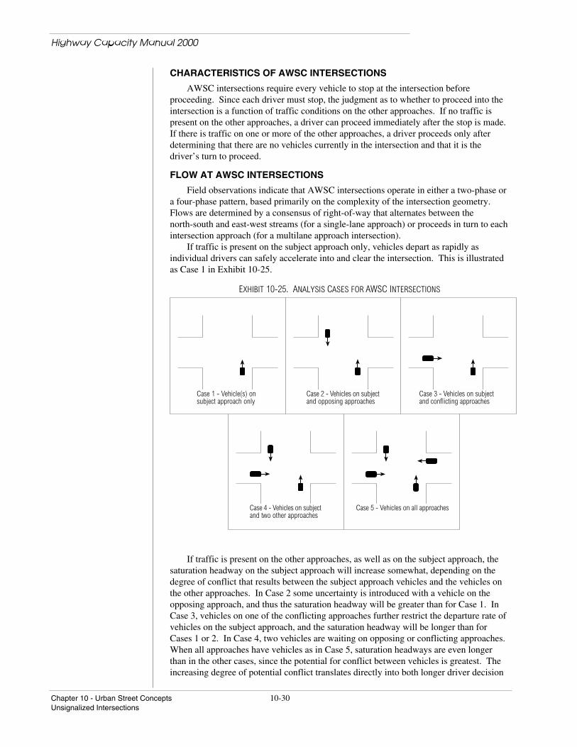
Highway Capacity Manual 2000
Chapter 10 - Urban Street Concepts 10-30Unsignalized Intersections
CHARACTERISTICS OF AWSC INTERSECTIONS
AWSC intersections require every vehicle to stop at the intersection beforeproceeding. Since each driver must stop, the judgment as to whether to proceed into theintersection is a function of traffic conditions on the other approaches. If no traffic ispresent on the other approaches, a driver can proceed immediately after the stop is made.If there is traffic on one or more of the other approaches, a driver proceeds only afterdetermining that there are no vehicles currently in the intersection and that it is thedriver’s turn to proceed.
FLOW AT AWSC INTERSECTIONS
Field observations indicate that AWSC intersections operate in either a two-phase ora four-phase pattern, based primarily on the complexity of the intersection geometry.Flows are determined by a consensus of right-of-way that alternates between thenorth-south and east-west streams (for a single-lane approach) or proceeds in turn to eachintersection approach (for a multilane approach intersection).
If traffic is present on the subject approach only, vehicles depart as rapidly asindividual drivers can safely accelerate into and clear the intersection. This is illustratedas Case 1 in Exhibit 10-25.
EXHIBIT 10-25. ANALYSIS CASES FOR AWSC INTERSECTIONS
Case 1 - Vehicle(s) onsubject approach only
Case 2 - Vehicles on subjectand opposing approaches
Case 3 - Vehicles on subjectand conflicting approaches
Case 4 - Vehicles on subjectand two other approaches
Case 5 - Vehicles on all approaches
If traffic is present on the other approaches, as well as on the subject approach, thesaturation headway on the subject approach will increase somewhat, depending on thedegree of conflict that results between the subject approach vehicles and the vehicles onthe other approaches. In Case 2 some uncertainty is introduced with a vehicle on theopposing approach, and thus the saturation headway will be greater than for Case 1. InCase 3, vehicles on one of the conflicting approaches further restrict the departure rate ofvehicles on the subject approach, and the saturation headway will be longer than forCases 1 or 2. In Case 4, two vehicles are waiting on opposing or conflicting approaches.When all approaches have vehicles as in Case 5, saturation headways are even longerthan in the other cases, since the potential for conflict between vehicles is greatest. Theincreasing degree of potential conflict translates directly into both longer driver decision

Highway Capacity Manual 2000
10-31 Chapter 10 - Urban Street ConceptsUnsignalized Intersections
times and saturation headways. Since no traffic signal controls the stream movement orallocates the right-of-way to each conflicting traffic stream, the rate of departure iscontrolled by the interactions between the traffic streams themselves.
CHARACTERISTICS OF ROUNDABOUTS
Three main features of roundabouts are illustrated in Exhibit 10-26: the centralisland, the circulating roadway, and the splitter island (10). A roundabout isdistinguished from a traffic circle in general by the following characteristics:
• Vehicles entering a roundabout are required to yield to vehicles within thecirculating roadway. Because of right-of-way constraints, some small traffic circles areunable to deflect vehicle paths properly to achieve the desired speed reduction.
• The circulating vehicles are not subjected to any other right-of-way conflicts, andweaving is kept to a minimum. This provides the means by which the priority isdistributed and alternated among vehicles. A vehicle entering as a subordinate vehicleimmediately becomes a priority vehicle until it exits the roundabout. Some traffic circlesimpose control measures within the circulating roadway or are designed with weavingareas to resolve conflicts between movements.
• Some small circles do not control speed because of the small central islanddiameter and because the radius of the vehicle path is large.
• No parking is allowed on the circulating roadway. Parking maneuvers, if allowed,would prevent the roundabout from operating in a manner consistent with its design.Some larger traffic circles permit parking within the circulating roadway.
• No pedestrian activities take place on the central island. Pedestrians are notexpected to cross the circulating roadway. Some larger traffic circles provide forpedestrians crossing to, and activities on, the central island.
• All vehicles circulate counterclockwise (in countries with a drive right policy),passing to the right of the central island. In some small traffic circles (sometimes calledmini–traffic circles) left-turning vehicles are expected to pass to the left of the centralisland.
• Roundabouts are designed to properly accommodate specified design vehicles.Some smaller traffic circles are unable to accommodate large vehicles, usually because ofright-of-way constraints.
• Roundabouts have raised splitter islands on all approaches. Splitter islands are anessential safety feature, required to separate traffic moving in opposite directions and toprovide refuge for pedestrians. Some smaller traffic circles do not provide raised splitterislands.
• When pedestrian crossings are provided for on the approach roads, they are placedapproximately one car length back from the entry point. Some traffic circlesaccommodate pedestrians in other places, such as the yield point.
• Vehicle speed into and through roundabouts is controlled by the physical featuresof a roundabout and not by signs or pavement markings.
PERFORMANCE MEASURES
Four measures are used to describe the performance of TWSC intersections: controldelay, delay to major street through vehicles, queue length, and v/c ratio. The primarymeasure that is used to provide an estimate of LOS is control delay. This measure can beestimated for any movement on the minor (i.e., the stop-controlled) street. By summingdelay estimates for individual movements, a delay estimate for each minor streetmovement and minor street approach can be achieved.
For AWSC intersections, the average control delay (in seconds per vehicle) is usedas the primary measure of performance. Control delay is the increased time of travel fora vehicle approaching and passing through an AWSC intersection, compared with a free-flow vehicle if it were not required to slow or stop at the intersection.
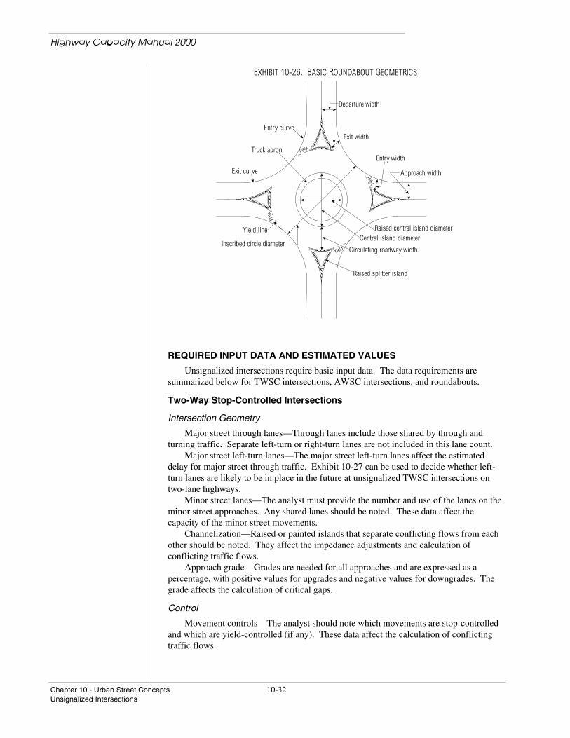
Highway Capacity Manual 2000
Chapter 10 - Urban Street Concepts 10-32Unsignalized Intersections
EXHIBIT 10-26. BASIC ROUNDABOUT GEOMETRICS
Central island diameter
Circulating roadway widthYield
Yield
Yield
Yield
Departure width
Exit widthEntry curve
Truck apron
Exit curve
Yield line
Inscribed circle diameter
Raised central island diameter
Approach width
Entry width
Raised splitter island
REQUIRED INPUT DATA AND ESTIMATED VALUES
Unsignalized intersections require basic input data. The data requirements aresummarized below for TWSC intersections, AWSC intersections, and roundabouts.
Two-Way Stop-Controlled Intersections
Intersection Geometry
Major street through lanes—Through lanes include those shared by through andturning traffic. Separate left-turn or right-turn lanes are not included in this lane count.
Major street left-turn lanes—The major street left-turn lanes affect the estimateddelay for major street through traffic. Exhibit 10-27 can be used to decide whether left-turn lanes are likely to be in place in the future at unsignalized TWSC intersections ontwo-lane highways.
Minor street lanes—The analyst must provide the number and use of the lanes on theminor street approaches. Any shared lanes should be noted. These data affect thecapacity of the minor street movements.
Channelization—Raised or painted islands that separate conflicting flows from eachother should be noted. They affect the impedance adjustments and calculation ofconflicting traffic flows.
Approach grade—Grades are needed for all approaches and are expressed as apercentage, with positive values for upgrades and negative values for downgrades. Thegrade affects the calculation of critical gaps.
Control
Movement controls—The analyst should note which movements are stop-controlledand which are yield-controlled (if any). These data affect the calculation of conflictingtraffic flows.

Highway Capacity Manual 2000
10-33 Chapter 10 - Urban Street ConceptsUnsignalized Intersections
EXHIBIT 10-27. MINIMUM APPROACH VOLUMES (veh/h) FOR LEFT-TURN LANES ON TWO-LANEHIGHWAYS AT UNSIGNALIZED INTERSECTIONS
Opposing Volume 5% Left Turns 10% Left Turns 20% Left Turns 30% Left Turns
Free-Flow Speed = 60 km/h
800 330 240 180 160600 410 305 225 200400 510 305 275 245200 640 470 350 305100 720 515 390 340
Free-Flow Speed = 80 km/h
800 280 210 165 135600 350 260 195 170400 430 320 240 210200 550 400 300 270100 615 445 335 295
Free-Flow Speed = 100 km/h
800 230 170 125 115600 290 210 160 140400 365 270 200 175200 450 330 250 215100 505 370 275 240
Source: AASHTO Policy on Geometric Design of Highways and Streets (1, p. 791).
Volumes
Turning movement volumes—The peak-hour turning volumes are required for allintersection approaches. Vehicle classification is used to calculate the percentage ofheavy vehicles.
Peak-hour factor (PHF)—The peak-hour volumes must be divided by the PHF beforebeginning the computations. If the analyst has peak 15-min flow rates, these flow ratescan be entered directly with the PHF set to 1.00.
Length of study period (T)—Refer to urban street description of length of studyperiod in this chapter under required input data and estimated values.
All-Way Stop-Controlled Intersections
Intersection Geometry
The number and configuration of lanes on each approach are used to determine thecomplexity of the analysis and to select applicable geometry groups.
Volumes
Turning movement volumes—Peak-hour turning volumes by movement for allintersection approaches are required, including vehicle classification (to calculate thepercentage of heavy vehicles).
Peak-hour factor (PHF)—The peak-hour volumes must be divided by the PHF beforebeginning the computations. If the analyst has peak 15-min flow rates, these flow ratescan be entered directly with the PHF set to 1.00.
Length of study period (T)—Refer to urban street description of length of studyperiod in this chapter under required data and estimated values.

Highway Capacity Manual 2000
Chapter 10 - Urban Street Concepts 10-34Unsignalized Intersections
Roundabouts
Intersection Geometry
The geometric layout of the intersection must be consistent with the characteristics ofa single-lane roundabout (see Chapter 17, “Unsignalized Intersections,” for details).
Volumes
Turning movement volumes—Peak-hour turning volumes by movement for allintersection approaches are required.
Peak-hour factor (PHF)—For the analysis to reflect conditions during the peak 15min, the peak-hour volumes must be divided by the PHF before beginning thecomputations. If the analyst has peak 15-min flow rates, these flow rates can be entereddirectly with the PHF set to 1.00.
SERVICE VOLUME TABLES
Exhibits 10-28 and 10-29 show the number of lanes required to achieve a desiredLOS for a TWSC intersection. The LOS shown in these example tables reflectsconditions for the worst movement at the intersections, which is usually the left turn fromthe stop-controlled minor street. These example service volumes reflect the specificassumptions listed in the exhibit footnotes. Exhibit 10-28 is for a T-intersection andgives example service volumes for a single-lane approach on the minor street. Exhibit10-29 gives example service volumes for four-leg intersections with varying laneconfigurations and two-way hourly volumes on the major street approaches rangingbetween 500 and 1,500 veh/h.
Exhibit 10-30 can be used to estimate the number of through lanes for each approachrequired to achieve a desired LOS for an AWSC intersection. Since the intersection isall-way stop controlled, each vehicle is required to stop before proceeding. Adding left-turn or right-turn pockets will not significantly reduce delay. The entries in the exhibitare maximum hourly approach volumes for any one of the four approaches to theintersection. These example service volumes reflect the specific assumptions found inthe exhibit footnotes.
EXHIBIT 10-28. EXAMPLE OF MINOR STREET SERVICE VOLUMES FOR T-INTERSECTIONTWO-WAY STOP INTERSECTION
(SEE FOOTNOTE FOR ASSUMED VALUES)This table containsapproximate values. It ismeant for illustrativepurposes only. Thevalues are highlydependent on theassumptions used. Itshould not be used foroperational analyses orfinal design. This tablewas derived usingassumed values listed inthe footnote.
LOS
Major Street2-Way Volume
A B C D E
(veh/h) Minor Street Approach Service Volumes for Single-Lane Approach (veh/h)
200 110 450 630 700 760400 N/A 280 460 530 590600 N/A 150 320 390 440800 N/A 40 210 270 320
1000 N/A N/A 120 180 230
Note:Assumptions: minor street left turns and right turns are equal; major street left turns and right turns are each 10% of theapproach volume; PHF = 0.92; heavy vehicles = 2%; grade = 0%; pedestrian flow = 0; no flared minor approach; nochannelization; 50/50 split of major street traffic; two-lane major street; major street left-turn pocket.N/A = not achievable under given conditions.
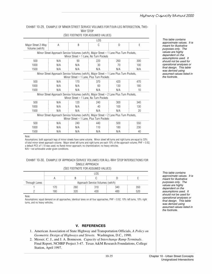
Highway Capacity Manual 2000
10-35 Chapter 10 - Urban Street ConceptsUnsignalized Intersections
EXHIBIT 10-29. EXAMPLE OF MINOR STREET SERVICE VOLUMES FOR FOUR-LEG INTERSECTION, TWO-WAY STOP
(SEE FOOTNOTE FOR ASSUMED VALUES)This table containsapproximate values. It ismeant for illustrativepurposes only. Thevalues are highlydependent on theassumptions used. Itshould not be used foroperational analyses orfinal design. This tablewas derived usingassumed values listed inthe footnote.
LOS
Major Street 2-WayVolume (veh/h)
A B C D E
Minor Street Approach Service Volumes (veh/h), Major Street = 1 Lane Plus Turn Pockets,Minor Street = 1 Lane, No Turn Pockets
500 N/A 90 220 260 3001000 N/A N/A 30 70 1001500 N/A N/A N/A N/A N/A
Minor Street Approach Service Volumes (veh/h), Major Street = 1 Lane Plus Turn Pockets,Minor Street = 1 Lane, Plus Turn Pockets
500 N/A 170 370 420 4701000 N/A N/A 60 130 1801500 N/A N/A N/A N/A 10
Minor Street Approach Service Volumes (veh/h), Major Street = 2 Lane Plus Turn Pockets,Minor Street = 1 Lane, No Turn Pockets
500 N/A 120 240 300 3401000 N/A N/A 40 100 1301500 N/A N/A N/A N/A 20
Minor Street Approach Service Volumes (veh/h), Major Street = 2 Lane Plus Turn Pockets,Minor Street = 1 Lane, Plus Turn Pockets
500 N/A 240 440 500 5501000 N/A N/A 110 180 2301500 N/A N/A N/A N/A 40
Note:Assumptions: both approach legs of minor streets have same volume. Minor street left turns and right turns are equal to 33%of total minor street approach volume. Major street left turns and right turns are each 10% of the approach volume; PHF = 0.92;a default PCE of 1.10 was used; no flared minor approach; no channelization; no heavy vehicles.N/A = not achievable under given conditions.
EXHIBIT 10-30. EXAMPLE OF APPROACH SERVICE VOLUMES FOR ALL-WAY STOP INTERSECTIONS FORSINGLE APPROACH
(SEE FOOTNOTE FOR ASSUMED VALUES)This table containsapproximate values. It ismeant for illustrativepurposes only. Thevalues are highlydependent on theassumptions used. Itshould not be used foroperational analyses orfinal design. This tablewas derived usingassumed values listed inthe footnote.
LOS
A B C D E
Through Lanes Approach Service Volumes (veh/h)
1 170 260 310 340 3502 180 320 430 480 520
Note:Assumptions: equal demand on all approaches, identical lanes on all four approaches, PHF = 0.92, 10% left turns, 10% rightturns, and no heavy vehicles.
V. REFERENCES
1. American Association of State Highway and Transportation Officials, A Policy onGeometric Design of Highways and Streets. Washington, D.C., 1990.
2. Messer, C. J., and J. A. Bonneson. Capacity of Interchange Ramp Terminals.Final Report, NCHRP Project 3-47. Texas A&M Research Foundations, CollegeStation, April 1997.

Chapter 10 - Urban Street Concepts 10-36References
3. Messer, C. J. Guidelines for Signalized Left-Turn Treatments, ImplementationPackage. FHWA-IP-81-4. Federal Highway Administration, U.S. Department ofTransportation, 1981.
4. Koepke, F. J., and H. S. Levinson. NCHRP Report 348: Access ManagementGuidelines for Activity Centers. TRB, National Research Council, Washington,D.C., 1992.
5. Harwood, D. W., M. T. Pietrucha, M. D. Wooldridge, R. E. Brydia, and K.Fitzpatrick. NCHRP Report 375: Median Intersection Design. TRB, NationalResearch Council, Washington, D.C., 1995.
6. Pedersen, N. J., and D. R. Samdahl. NCHRP Report 255: Highway Traffic Datafor Urbanized Area Project Planning and Design. TRB, National ResearchCouncil, Washington, D.C., 1982, specifically citing Mekky, A., On EstimatingTurning Flows at Road Junctions, Traffic Engineering and Control Journal, Vol.20:10, October 1979, pp. 486-487.
7. Ortuzar, J. D., and L. G. Willumsen. Modeling Transport, 2nd ed. John Wileyand Sons, New York, 1994.
8. Traffic Control Devices Handbook. Federal Highway Administration, U.S.Department of Transportation, 1983.
9. Kittelson, W. K., and M. A. Vandehey. Delay Effects on Driver Gap AcceptanceCharacteristics at Two-Way Stop-Controlled Intersections. In TransportationResearch Record 1320, TRB, National Research Council, Washington, D.C., 1991,pp. 154–159.
10. Kyte, M., Z. Tian, Z. Mir, Z. Hameedmansoor, W. Kittelson, M. Vandehey, B.Robinson, W. Brilon, L. Bondzio, N. Wu, and R. Troutbeck. Capacity and Levelof Service at Unsignalized Intersections. Final Report, NCHRP Project 3-46.April 1996.
APPENDIX A. QUICK ESTIMATION METHOD FOR SIGNALIZEDINTERSECTIONS
Xc is the measure ofeffectiveness for quickestimation methods
A quick estimation method for determining the critical v/c ratio, Xc, signal timing,and delay for a signalized intersection is described in this appendix. This procedure canbe used when only minimal data are available for the analysis and only approximateresults are desired.
The quick estimation method consists of six steps: assembly of the input data,determination of left-turn treatment, lane volume computations, estimation of signaltiming plan, calculation of the critical v/c ratio, and calculation of average vehicle delay.
INPUT REQUIREMENTS
The overall data requirements are summarized in Exhibit A10-1. The inputworksheet is shown in Exhibit A10-2. Some of the input requirements may be met byassumed values or default values that represent reasonable values for operatingparameters. Other data items are site specific and must be obtained in the field. Theobjective of using the quick estimation method is to minimize the need for collection ofdetailed field data.
The calculations integrated into the quick estimation method and specificallyindicated in the worksheets include several default values for variables. The values havebeen selected to be generally representative and to simplify the analysis. Thecomputations for the quick estimation method must be based on the traffic volumes andlane configuration of each approach to the intersection.
The worksheets for computation are shown in Exhibits A10-2, A10-3, A10-4, andA10-5. The first step is to input geometric data and all volume-related parameters on the
Highway Capacity Manual 2000

Highway Capacity Manual 2000
10-37 Chapter 10 - Urban Street ConceptsAppendix A
input worksheet. Critical lane volume (VCL) and left-turn volume (VLT) are obtained
according to the method discussed below.
EXHIBIT A10-1. INPUT DATA REQUIREMENTS FOR QUICK ESTIMATION METHOD
Data Item Comments
Volumes By movement as projectedLanes Left, through, or right; exclusive or sharedAdjusted saturation flow rate Includes all adjustments for PHF, CBD, grades, etc.Left-turn treatment (phasing plan) Use actual treatment, if known. See discussion of
phasing plan development.Cycle length (min and max) Use actual value, if known. May be estimated using
signal operations worksheet.Lost time May be estimated using signal operations worksheetGreen times Use actual values, if known. May be estimated using
signal operations worksheet.Coordination Isolated intersection versus intersection influenced by
upstream signalsPeak-hour factor Use default value of 0.90 if not knownParking On-street parking is or is not presentArea type Signal is or is not in CBD
DETERMINATION OF LEFT-TURN TREATMENTDo not use this quickestimation method as the solebasis for determining need forprotected left-turn phasing
The signal timing needs of permitted left turns are not considered in the syntheses ofthe traffic signal timing plan in the quick estimation technique. Therefore, failure toassume protected left-turn phases for heavy left-turn flow rates will generally produce anoverly optimistic assessment of the critical v/c ratio and intersection operations.
Exhibit A10-3 provides a procedure for determining whether a permitted left turnshould be protected instead in the quick estimation of intersection operations. This left-turn treatment check is not necessary if the left turn is unopposed or if the analyst wishesto analyze only protected left turns. Above all, the left-turn treatment checks should notbe used as the sole determinant of the need for protected left-turn phasing.
Even if the analyst already knows that permitted left-turn treatment will beimplemented, this left-turn treatment check must still be used to check that the left-turntreatment does not conflict with the assumptions on which this quick estimation methodis based. The more robust methodology presented in Chapter 16, “SignalizedIntersections,” should be used whenever the analyst wishes to analyze an intersectionwith permitted left turns that fails the left-turn treatment checks in Exhibit A10-3.
The determination of the recommended left-turn treatment is accomplished in foursteps. The first step recommends left-turn protection if there is more than one left-turnlane on the approach. The second step recommends left-turn protection if there are morethan 240 veh/h (unadjusted) turning left. The third step recommends left-turn protectionif the cross-product of the unadjusted left turn and opposing mainline volumes exceedsthe minimum values shown in Exhibit A10-3. The opposing mainline volume is usuallythe summation of the opposing through and right-turning vehicles. If the analystrecognizes that the opposing approach geometry is such that left-turn vehicles can safelyignore the opposing right-turn vehicles, the opposing right-turn vehicles can be excluded.Such situations occur if there is an exclusive right-turn lane on the opposing approach andthe right-turning vehicles have their own lane to turn into on the cross street withoutinterfering with the left-turning vehicles.
The final step compares the left-turn demand with the average number that can sneakthrough on the yellow phase and recommends left-turn protection if the opposing flowsare high enough to result in a left-turn equivalence factor (computed later) exceeding 3.5.

Highway Capacity Manual 2000
Chapter 10 - Urban Street Concepts 10-38Appendix A
Once it is determined that left-turn protection is recommended for a given approach, thesubsequent checks for that approach are unnecessary.
EXHIBIT A10-2. QUICK ESTIMATION INPUT WORKSHEET
Volume and Signal Input
Show North
Stre
et
Street
Notes
Peak-hour factor, PHF ________
Cycle length Minimum, Cmin ______ s Maximum, Cmax ______ s or Given, C ______ s
Lost time/phase ________s
1. RT volumes, as shown, exclude RTOR.
2. PLT = 1.000 for exclusive left-turn lanes, and PRT = 1.000 for exclusive right-turn lanes. Otherwise, they are equal to the proportions of turningvolumes in the lane group.
QUICK ESTIMATION INPUT WORKSHEET
EB WB NB SB
LT TH RT1 LT TH RT1 LT TH RT1 LT TH RT1
Volume, V (veh/h)
Proportion of LT or RT (PLT or PRT)2 - - - -
Parking (Yes/No)
Left-turn treatment (permitted, protected,not opposed) (if known)
= Through
= Right
= Left
= Through + Right
= Left + Through
= Left + Right
= Left + Through + Right
Analyst ________________________ Intersection __________________________
Agency or Company ___________________________ Area Type � CBD � Other
Date Performed ___________________________ Jurisdiction ____________________________
Analysis Time Period ___________________________ Analysis Year _____________________________
General Information Site Information
Intersection Geometry
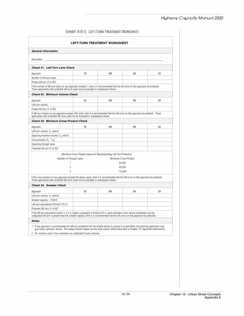
EXHIBIT A10-3. LEFT-TURN TREATMENT WORKSHEET
LEFT-TURN TREATMENT WORKSHEET
General Information
Description ______________________________________________________________________________________
Check #1. Left-Turn Lane Check
Approach EB WB NB SB
Number of left-turn lanes
Protect left turn (Y or N)?
If the number of left-turn lanes on any approach exceeds 1, then it is recommended that the left turns on that approach be protected.Those approaches with protected left turns need not be evaluated in subsequent checks.
Check #2. Minimum Volume Check
Approach EB WB NB SB
Left-turn volume
Protect left turn (Y or N)?
If left-turn volume on any approach exceeds 240 veh/h, then it is recommended that the left turns on that approach be protected. Thoseapproaches with protected left turns need not be evaluated in subsequent checks.
Check #3. Minimum Cross-Product Check
Approach EB WB NB SB
Left-turn volume, VL (veh/h)
Opposing mainline volume, Vo (veh/h)
Cross-product (VL * Vo)
Opposing through lanes
Protected left turn (Y or N)?
Minimum Cross-Product Values for Recommending Left-Turn Protection
Number of Through Lanes Minimum Cross-Product
1 50,000
2 90,000
3 110,000
If the cross-product on any approach exceeds the above values, then it is recommended that the left turns on that approach be protected.Those approaches with protected left turns need not be evaluated in subsequent checks.
Check #4. Sneaker Check
Approach EB WB NB SB
Left-turn volume, VL (veh/h)
Sneaker capacity = 7200/C
Left-turn equivalence (Exhibit C16-3)
Protected left turn (Y or N)?
If the left-turn equivalence factor is 3.5 or higher (computed in Exhibit A10-4, quick estimation lane volume worksheet) and theunadjusted left turn is greater than the sneaker capacity, then it is recommended that the left turns on that approach be protected.
Notes
1. If any approach is recommended for left-turn protection but the analyst wishes to analyze it as permitted, the planning application maygive overly optimistic results. The analyst should instead use the more robust method described in Chapter 16, Signalized Intersections.
2. All volumes used in this worksheet are unadjusted hourly volumes.
10-39 Chapter 10 - Urban Street ConceptsAppendix A
Highway Capacity Manual 2000

Highway Capacity Manual 2000
Chapter 10 - Urban Street Concepts 10-40Appendix A
EXHIBIT A10-4. QUICK ESTIMATION LANE VOLUME WORKSHEET
General Information
Right-Turn Movement
Left-Turn Movement
Through Movement
Through Movement with Exclusive LT Lane
Through Movement with Shared LT Lane
Notes
QUICK ESTIMATION LANE VOLUME WORKSHEET
Description/Approach ________________________________________________________________________________
Exclusive RT Lane Shared RT Lane
RT volume, VR (veh/h)
Number of exclusive RT lanes, NRT use 1
RT adjustment factor,1 fRT
RT volume per lane, VRT (veh/h/ln)VRT =
LT volume, VL (veh/h)
Opposing mainline volume, Vo (veh/h)
Number of exclusive LT lanes, NLT
LT adjustment factor,2 fLT
LT volume per lane,3 VLT (veh/h/ln)
VLT = Permitted LT _______ Protected LT _______ Not Opposed LT ______
Permitted LT Protected LT Not Opposed LT
Through volume, VT (veh/h)
Parking adjustment factor, fpNumber of through lanes, NTH
Total approach volume,4 Vtot (veh/h)
Vtot =
Through volume per lane, VTH (veh/h/ln)
VTH =
Critical lane volume,5 VCL (veh/h)Max[VLT, VRT (exclusive), VTH]
use 0
Does not apply Does not apply
Does not apply Does not apply
use 1.0
Proportion of left turns, PLT
LT equivalence, EL1 (Exhibit C16-3)
LT adjustment, fDL (Exhibit A10-6)
Through volume per lane, VTH (veh/h/ln)VTH =
Critical lane volume,5 VCL (veh/h)Max[VRT(exclusive), VTH]
1. For RT shared or single lanes, use 0.85. For RT double lanes, use 0.75.2. For LT single lanes, use 0.95. For LT double lanes, use 0.92. For a one-way street or T-intersection, use 0.85 for one lane and 0.75
for two lanes.3. For unopposed LT shared lanes, NLT = 1.4. For exclusive RT lanes, VRT (shared) = 0. If not opposed, add VLT to VT and set VLT (not opp) = 0.5. VLT is included only if LT is unopposed. VRT (exclusive) is included only if RT is exclusive.
Vtot
(NTH x fDL)
Vtot
NTH
VL
(NLT x fLT)
VR
(NRT x fRT)
[VRT(shared) + VT + VLT (not opp)]
fp

10-41 Chapter 10 - Urban Street ConceptsAppendix A
EXHIBIT A10-5. QUICK ESTIMATION CONTROL DELAY AND LOS WORKSHEET
Selected plan (Exhibit A10-8) _________ Phase No. 1 Phase No. 2 Phase No. 3Movement codesCritical phase volume, CV (veh/h)Lost time/phase, tL (s)
Selected plan (Exhibit A10-8) _________ Phase No. 1 Phase No. 2 Phase No. 3Movement codesCritical phase volume, CV (veh/h)Lost time/phase, tL (s)
EB WB NB SB
Lane group
Lane group adjusted volume from lane volumeworksheet, V (veh/h)
Green ratio, g/C
Lane group saturation flow rate, s (veh/h)s = RS * number of lanes in lane group
v/c ratio, X
Lane group capacity, c (veh/h)
Progression adjustment factor, PF (Exhibit 16-12)
Uniform delay, d1 (s/veh) (Equation 16-11)
Incremental delay, d2 (s/veh) (Equation 16-12)
Initial queue delay, d3 (s/veh) (Appendix F, Ch. 16)
Delay, d = d1(PF) + d2 + d3 (s/veh)
Delay by approach, dA (s/veh)
Approach flow rate, VA (veh/h)
Intersection delay, dI (s/veh)
Description________________________________________________________________________________________
QUICK ESTIMATION CONTROL DELAY AND LOS WORKSHEET
General Information
East-West Phasing Plan
North-South Phasing Plan
Intersection Status Computation
Control Delay and LOS
Green Time Calculation
Notes
1. RS = 1530(PHF)(fa), where fa is area adjustment factor (0.90 for CBD and 1.0 for all others).
Critical sum, CS (veh/h) CS = ∑CVLost time/cycle, L (s) L = ∑ tLReference sum flow rate RS (veh/h)1
Cycle length, C (s)Cmin ≤ C ≤ CmaxC = Cmax when CS ≥ RS
Critical v/c ratio, Xc
Intersection status (Exhibit A10-9)
East-West Phasing Phase No. 1 Phase No. 2 Phase No. 3
Green time, g (s)
North-South Phasing Phase No. 1 Phase No. 2 Phase No. 3
Green time, g (s)
Intersection LOS (Exhibit 16-2)
g = (C – L) + tL( )CVCS
g = (C – L) + tL( )CVCS
V/sg/C
X =
VX
c =
∑(d)(V)∑V
∑(dA)(VA)∑VA
dI =
L
1 –C =
CSRS
LC
1 –(1700*PHF*fa)
CSXc =
( )
Highway Capacity Manual 2000

Highway Capacity Manual 2000
Chapter 10 - Urban Street Concepts 10-42Appendix A
LANE VOLUME COMPUTATIONS
The purpose of the lane volume worksheet (Exhibit A10-4) is to establish theindividual lane flow rates (in veh/h/ln) on all approaches. This information is used on thecontrol delay and LOS worksheet to synthesize the signal timing plan. The lane volumeworksheet contains additional items such as left-turn treatment alternatives, parkingadjustments, left-turn equivalence, and adjustment factors for shared lanes with permittedleft turns. The directional designations refer to the movements as they approach theintersection.
Each of the three left-turn treatment alternatives identified must be processeddifferently in computing the lane volumes. Therefore, the lane volume worksheetcontains three columns, each representing one of the alternatives. Only one of the threecolumns should be used for each approach. The following instructions cover theprocedure for completing all of the items on the lane volume worksheet.
Right-turn volumes (veh/h) (with the estimated right-turn-on-red volume having beenremoved from the total) from either a shared through and right-turn lane or from anexclusive turn lane should be entered. The right-turn adjustment factor is 0.85 for asingle lane or a shared lane and 0.75 for two lanes. The total right-turn volume should bedivided by the product of the number of exclusive right-turn lanes and the right-turnadjustment factor.
Left-turn flow rate isadjusted for left-turnsneakers
The next worksheet computation involves the left-turn volume. In the case ofprotected-plus-permitted phasing with an exclusive left-turn lane, two vehicles per cycleshould be removed from the left-turn volume to account for the effect of sneakers. If thecycle length has not been established, the maximum allowable cycle length should beused. To prevent unreasonably short protected left-turn phases, this volume adjustmentstep should not reduce the left-turn volume to a value below four vehicles per cycle. Theopposing mainline volume is the total approach volume minus the left-turn volume fromexclusive lanes or from a single lane (veh/h). The number of exclusive left-turn lanes isthe number of lanes exclusively designated to accommodate the left-turn volumes. Theleft-turn adjustment factor applies only to protected left turns from exclusive left-turnlanes or to left turns that are not opposed. This factor is given as 0.95 for single lanes and0.92 for double lanes. If the left-turn movement is not opposed because of a one-waystreet or T-intersection, pedestrian interference must be considered. The correspondingvalue of 0.85 for one lane and 0.75 for two lanes is used. The total left-turn volume isdivided by the product of the number of exclusive left-turn lanes and the left-turnadjustment factor. The left-turn volume is entered directly if there is no exclusive left-turn lane. The result is expressed in units of veh/h/ln. Zero should always be entered ifthe left turns are permitted.
Total through volume for the approach, excluding left and right turns, is placed in theappropriate row to correspond to the applicable treatment for left turns (permitted,protected, or not opposed). The parking adjustment factor and the number of throughlanes are noted. Exclusive turn lanes should be excluded. For an unopposed shared lane,the total approach volume is the sum of the shared-lane right-turn volume, the throughvolume, and the left-turn volume. Through-lane volume is then computed by dividingtotal approach volume by the number of through lanes. Critical lane volume is normallythe same as through-lane volume, unless the right turn has an exclusive lane or the leftturn is not opposed and either of these movements is more critical than the throughmovement. If both conditions apply, the critical lane volume will be the largest of theleft-lane volume, exclusive right-lane volume, and through-lane volume.
The computation of critical lane volume in the case of shared left-turn lanes is morecomplicated and requires a more detailed computational procedure. The total approachvolume is computed in nearly the same manner as for exclusive left-turn lanes. Theproportion of left turns in a lane group is self-explanatory. Left-turn equivalence is oneof the factors needed to compute the applicable formulas in Appendix C of Chapter 16 forshared-lane permitted left turns. It is not used at all when the left turn is protected. The

Highway Capacity Manual 2000
10-43 Chapter 10 - Urban Street ConceptsAppendix A
left-turn adjustment factor for through traffic, fDL, is computed according to ExhibitA10-6. This reduction factor is applied to the through volumes to account for the effectof left-turning vehicles waiting for a gap in the opposing traffic to make the turn. Notethat for lanes that are not opposed, the factor is 1.0 because these vehicles will have gapsthrough which to turn.
EXHIBIT A10-6. SHARED-LANE, LEFT-TURN ADJUSTMENT COMPUTATION FOR QUICK ESTIMATION
Permitted Left Turn
Lane groups with two or more lanes: Subject to a minimum value that applies at very lowleft-turning volumes when some cycles will have noleft-turn arrivals:
fDL = (NTH −1) + e
−NTHVLEL1
600
NTH
fDL(min) = (NTH −1) + e
−VLCmax
3600
NTH
Lane groups with only one lane for all movements:
fDL = e−0 .02 (EL1 +10PLT )
VLCmax
3600
Protected-Plus-Permitted Left Turn (one direction only)
If Vo < 1220 If Vo ≥ 1220
fDL = 1
1 +PLT 235 + 0.435Vo( )
1400 −Vo
fDL = 11 + 4.525PLT
The through-lane volume is then computed. Note that the number of lanes is reducedby the shared left-turn adjustment factor to account for the effect of the left-turningvehicles.
In the exclusive left-turn lane case, the critical lane volume is the maximum of eitherthe through-lane volume or the right-turn volume from an exclusive right-turn lane. Ifone or more left turns have been designated as permitted (i.e., no protected phase hasbeen assigned), the need for a protected phase should be reexamined at this point.
As indicated in Chapter 16, Appendix C, values for the left-turn equivalence above3.5 imply that left-turn capacity is derived substantially from sneakers. Therefore, if theleft-turn equivalence is greater than 3.5 and the left-turn volume is greater than twovehicles per cycle, it is likely that the subject left turn will not have adequate capacitywithout a protected phase.
SIGNAL TIMING ESTIMATION
The purpose of this step is to estimate a feasible signal timing plan for theintersection. The signal timing plan is required to estimate delay. Note that the signaltiming plan estimated using the method described below is not necessarily the optimaltiming plan. The timing plan is estimated in five substeps: phasing plan development,computation of critical sum, estimation of total lost time, cycle length estimation, andeffective green time estimation.
Phasing Plan Development
The phase plan is selected from six alternatives presented in Exhibit A10-7. If thephasing plan is not known, the selection is made on the basis of the user-specified left-turn protection and the dominant left-turn movements identified from the left-turntreatment worksheet (Exhibit A10-3).
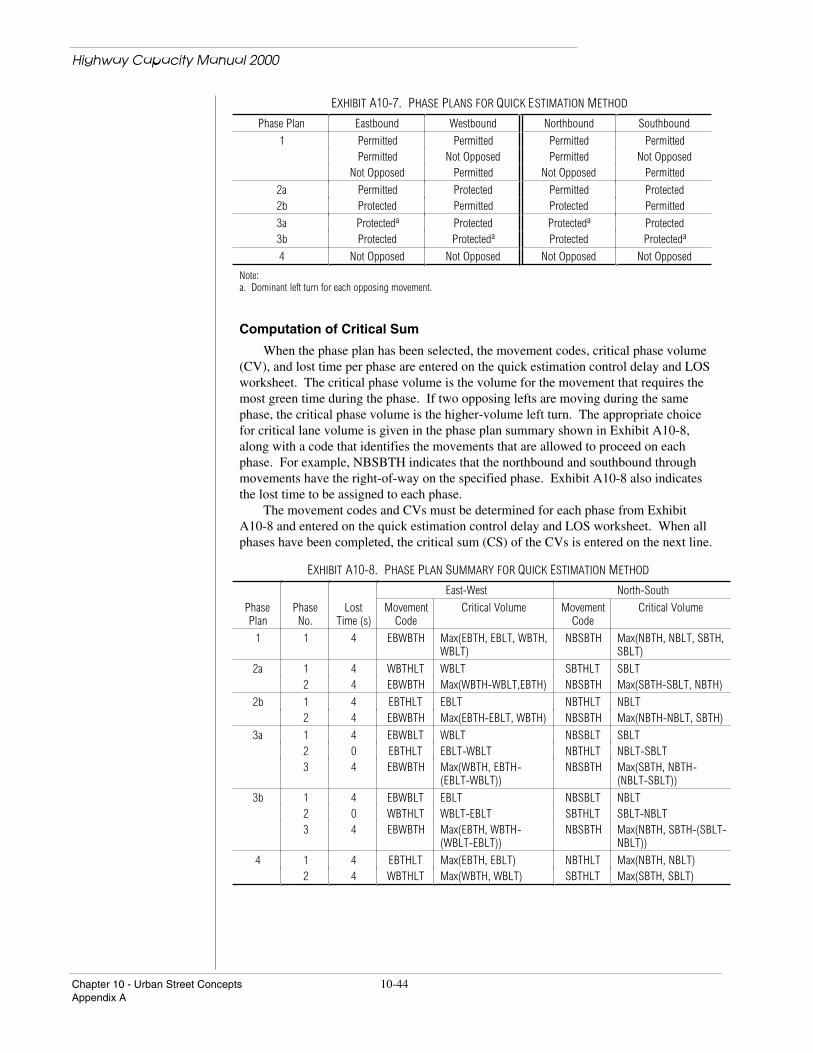
Highway Capacity Manual 2000
Chapter 10 - Urban Street Concepts 10-44Appendix A
EXHIBIT A10-7. PHASE PLANS FOR QUICK ESTIMATION METHOD
Phase Plan Eastbound Westbound Northbound Southbound
1 Permitted Permitted Permitted PermittedPermitted Not Opposed Permitted Not Opposed
Not Opposed Permitted Not Opposed Permitted
2a Permitted Protected Permitted Protected2b Protected Permitted Protected Permitted
3a Protecteda Protected Protecteda Protected3b Protected Protecteda Protected Protecteda
4 Not Opposed Not Opposed Not Opposed Not Opposed
Note:a. Dominant left turn for each opposing movement.
Computation of Critical Sum
When the phase plan has been selected, the movement codes, critical phase volume(CV), and lost time per phase are entered on the quick estimation control delay and LOSworksheet. The critical phase volume is the volume for the movement that requires themost green time during the phase. If two opposing lefts are moving during the samephase, the critical phase volume is the higher-volume left turn. The appropriate choicefor critical lane volume is given in the phase plan summary shown in Exhibit A10-8,along with a code that identifies the movements that are allowed to proceed on eachphase. For example, NBSBTH indicates that the northbound and southbound throughmovements have the right-of-way on the specified phase. Exhibit A10-8 also indicatesthe lost time to be assigned to each phase.
The movement codes and CVs must be determined for each phase from ExhibitA10-8 and entered on the quick estimation control delay and LOS worksheet. When allphases have been completed, the critical sum (CS) of the CVs is entered on the next line.
EXHIBIT A10-8. PHASE PLAN SUMMARY FOR QUICK ESTIMATION METHOD
East-West North-South
PhasePlan
PhaseNo.
LostTime (s)
MovementCode
Critical Volume MovementCode
Critical Volume
1 1 4 EBWBTH Max(EBTH, EBLT, WBTH,WBLT)
NBSBTH Max(NBTH, NBLT, SBTH,SBLT)
2a 1 4 WBTHLT WBLT SBTHLT SBLT2 4 EBWBTH Max(WBTH-WBLT,EBTH) NBSBTH Max(SBTH-SBLT, NBTH)
2b 1 4 EBTHLT EBLT NBTHLT NBLT2 4 EBWBTH Max(EBTH-EBLT, WBTH) NBSBTH Max(NBTH-NBLT, SBTH)
3a 1 4 EBWBLT WBLT NBSBLT SBLT2 0 EBTHLT EBLT-WBLT NBTHLT NBLT-SBLT3 4 EBWBTH Max(WBTH, EBTH-
(EBLT-WBLT))NBSBTH Max(SBTH, NBTH-
(NBLT-SBLT))
3b 1 4 EBWBLT EBLT NBSBLT NBLT2 0 WBTHLT WBLT-EBLT SBTHLT SBLT-NBLT3 4 EBWBTH Max(EBTH, WBTH-
(WBLT-EBLT))NBSBTH Max(NBTH, SBTH-(SBLT-
NBLT))
4 1 4 EBTHLT Max(EBTH, EBLT) NBTHLT Max(NBTH, NBLT)2 4 WBTHLT Max(WBTH, WBLT) SBTHLT Max(SBTH, SBLT)
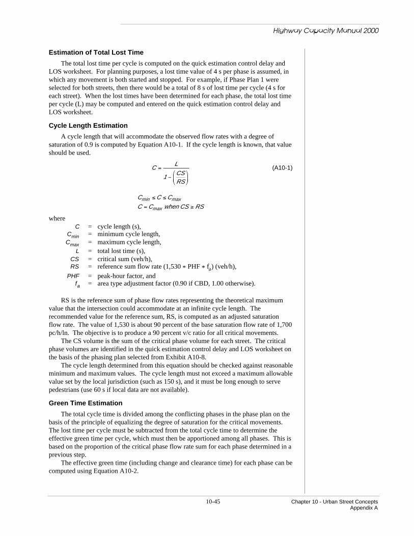
10-45 Chapter 10 - Urban Street ConceptsAppendix A
Estimation of Total Lost Time
The total lost time per cycle is computed on the quick estimation control delay andLOS worksheet. For planning purposes, a lost time value of 4 s per phase is assumed, inwhich any movement is both started and stopped. For example, if Phase Plan 1 wereselected for both streets, then there would be a total of 8 s of lost time per cycle (4 s foreach street). When the lost times have been determined for each phase, the total lost timeper cycle (L) may be computed and entered on the quick estimation control delay andLOS worksheet.
Cycle Length Estimation
A cycle length that will accommodate the observed flow rates with a degree ofsaturation of 0.9 is computed by Equation A10-1. If the cycle length is known, that valueshould be used.
C =L
1 −CSRS
(A10-1)
Cmin ≤ C ≤ Cmax
C =Cmax when CS ≥ RS
whereC = cycle length (s),
Cmin = minimum cycle length,Cmax = maximum cycle length,
L = total lost time (s),CS = critical sum (veh/h),RS = reference sum flow rate (1,530 * PHF * fa) (veh/h),
PHF = peak-hour factor, andfa = area type adjustment factor (0.90 if CBD, 1.00 otherwise).
RS is the reference sum of phase flow rates representing the theoretical maximumvalue that the intersection could accommodate at an infinite cycle length. Therecommended value for the reference sum, RS, is computed as an adjusted saturationflow rate. The value of 1,530 is about 90 percent of the base saturation flow rate of 1,700pc/h/ln. The objective is to produce a 90 percent v/c ratio for all critical movements.
The CS volume is the sum of the critical phase volume for each street. The criticalphase volumes are identified in the quick estimation control delay and LOS worksheet onthe basis of the phasing plan selected from Exhibit A10-8.
The cycle length determined from this equation should be checked against reasonableminimum and maximum values. The cycle length must not exceed a maximum allowablevalue set by the local jurisdiction (such as 150 s), and it must be long enough to servepedestrians (use 60 s if local data are not available).
Green Time Estimation
The total cycle time is divided among the conflicting phases in the phase plan on thebasis of the principle of equalizing the degree of saturation for the critical movements.The lost time per cycle must be subtracted from the total cycle time to determine theeffective green time per cycle, which must then be apportioned among all phases. This isbased on the proportion of the critical phase flow rate sum for each phase determined in aprevious step.
The effective green time (including change and clearance time) for each phase can becomputed using Equation A10-2.
Highway Capacity Manual 2000

Chapter 10 - Urban Street Concepts 10-46Appendix A
g = (C − L)CVCS
(A10-2)
whereg = effective green time (s),
CV = critical phase flow rate (veh/h),CS = critical sum (veh/h),
C = cycle length (s), andL = total lost time per cycle (s).
The analyst should note that this method of estimating green time will not necessarilyminimize the overall delay at the intersection.
COMPUTATION OF CRITICAL v/c RATIO
The critical v/c ratio, Xc, is an approximate indicator of the overall sufficiency of theintersection geometrics. The computational method involves the summation ofconflicting critical lane flow rates for the intersection. The computations depend ontraffic signal phasing, which in turn depends on the type of protection assigned to eachleft-turn movement. The quick estimation critical v/c ratio, Xc, is the ratio of the criticalsum, CS, to the sum of the critical lane flow rates that can accommodate demand at thegiven cycle length and is computed by Equation A10-3.
Xc =CS
1700 * PHF * f a( ) 1 −LC
(A10-3)
whereXc = critical v/c ratio,
CS = critical sum (veh/h),PHF = peak-hour factor,
fa = area type adjustment factor (0.90 if CBD, 1.00 otherwise),L = total lost time (s), andC = cycle length (s).
The critical sum is the sum of the critical phase volumes per lane at the intersection.A phasing plan identifying the protected left turns at the intersection must be known ordeveloped for the intersection to compute the critical sum. The computation of thecritical phase volumes per lane and the critical sum and the development of an estimatedphasing plan are described in the section on the estimation of a signal timing plan.
The reference sum was derived on the basis of minimum acceptable operationalconditions and typical traffic flow conditions. More refined saturation flow rates arecomputed by using the methodology of Chapter 16.
Although it is not appropriate to assign an LOS to the intersection on the basis of Xc,it is appropriate to evaluate the operational status of the intersection for quick estimationpurposes. Exhibit A10-9 expresses the intersection status as over, at, near, or undercapacity.
EXHIBIT A10-9. INTERSECTION STATUS CRITERIA FOR QUICK ESTIMATION METHOD
Critical v/c Ratio (Xc) Relationship to Capacity
Xc ≤ 0.85 Under capacity> 0.85 - 0.95 Near capacity> 0.95 - 1.00 At capacity
Xc > 1.00 Over capacity
Highway Capacity Manual 2000

10-47 Chapter 10 - Urban Street ConceptsAppendix A
COMPUTATION OF DELAY
First, the lane groups are established for all approaches. Lane grouping is explainedin Chapter 16. Exhibit 16-5 shows different types of lane groups for analysis. Lanegroup volumes are computed by summing the adjusted volumes obtained from the quickestimation lane volume worksheet (Exhibit A10-4) for each lane group on each approach.The green ratio (g/C) is computed using green time and cycle length values from the topportion of the quick estimation control delay and LOS worksheet. The lane groupsaturation flow rate is equal to the reference sum times the number of lanes in the lanegroup. The lane group v/c ratio is calculated using adjusted lane group volumes and lanegroup saturation flow rates computed previously and g/C ratios. Lane group capacity iscalculated using lane group adjusted volumes and lane group v/c ratios. The progressionadjustment factor for uniform delay calculation, PF, is selected from Exhibit 16-12. Forquick estimation purposes, the analyst may assume Arrival Type 3 for an uncoordinatedsignal and Arrival Type 4 for coordinated operation (for coordinated lane groups only).
The final step is to compute the various components of control delay using Equations16-10 through 16-14 in Chapter 16, “Signalized Intersections.” This chapter providesguidance on selecting default values for parameters used in the delay equations. Delay byapproach, approach volumes, and intersection delay require the delay to be averagedacross actual volumes on the quick estimation method input worksheet, not adjustedvolumes used to compute capacity. The values VA and V used in these equations should
be computed using unadjusted volumes that are inputs on the quick estimation methodinput worksheet.
Note that this procedure does not provide sufficient information for the computationof delay for permitted left turns from an exclusive turn lane. The analyst may ignore thisdelay in the computations or may use the more detailed capacity and LOS procedureprovided in Chapter 16, “Signalized Intersections.” In addition, the quick estimationmethod does not include the delay associated with the two sneakers per cycle, which hasbeen subtracted from the left-turn volumes for permitted and protected/permitted leftturns.
APPENDIX B. WORKSHEETS
QUICK ESTIMATION INPUT WORKSHEET
LEFT-TURN TREATMENT WORKSHEET
QUICK ESTIMATION LANE VOLUME WORKSHEET
QUICK ESTIMATION CONTROL DELAY AND LOS WORKSHEET
Highway Capacity Manual 2000

Chapter 10 - Urban Street Concepts
Highway Capacity Manual 2000
= Through
= Right
= Left
= Through + Right
= Left + Through
= Left + Right
= Left + Through + Right
Volume and Signal Input
Show NorthSt
reet
Street
Notes
QUICK ESTIMATION INPUT WORKSHEET
EB WB NB SB
LT TH RT1 LT TH RT1 LT TH RT1 LT TH RT1
Volume, V (veh/h)
Proportion of LT or RT (PLT or PRT)2 - - - -
Parking (Yes/No)
Left-turn treatment (permitted, protected,not opposed) (if known)
Analyst ________________________ Intersection __________________________
Agency or Company ___________________________ Area Type � CBD � Other
Date Performed ___________________________ Jurisdiction ____________________________
Analysis Time Period ___________________________ Analysis Year _____________________________
General Information Site Information
Intersection Geometry
Peak-hour factor, PHF ________
Cycle length Minimum, Cmin ______ s Maximum, Cmax ______ s or Given, C ______ s
Lost time/phase ________s
1. RT volumes, as shown, exclude RTOR.
2. PLT = 1.000 for exclusive left-turn lanes, and PRT = 1.000 for exclusive right-turn lanes. Otherwise, they are equal to the proportions of turningvolumes in the lane group.
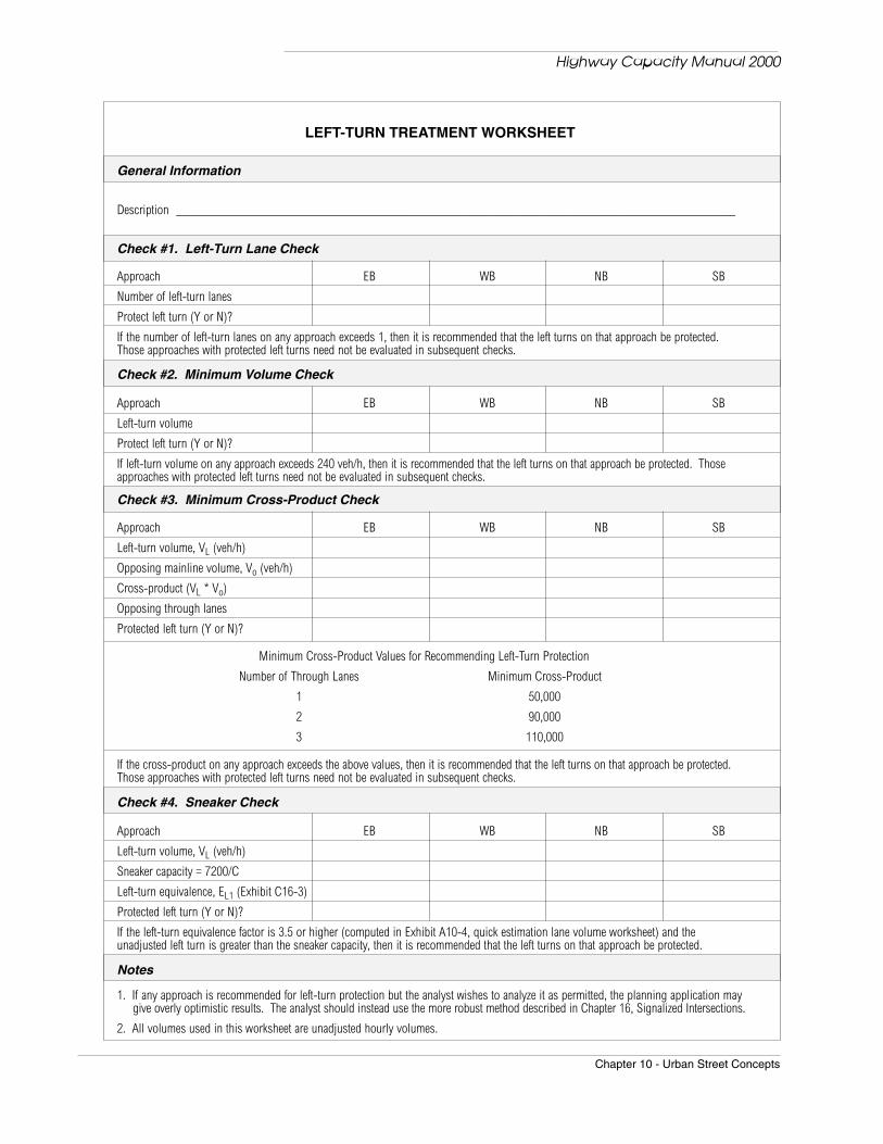
Chapter 10 - Urban Street Concepts
Highway Capacity Manual 2000
LEFT-TURN TREATMENT WORKSHEET
General Information
Description ______________________________________________________________________________________
Check #1. Left-Turn Lane Check
Approach EB WB NB SB
Number of left-turn lanes
Protect left turn (Y or N)?
If the number of left-turn lanes on any approach exceeds 1, then it is recommended that the left turns on that approach be protected.Those approaches with protected left turns need not be evaluated in subsequent checks.
Check #2. Minimum Volume Check
Approach EB WB NB SB
Left-turn volume
Protect left turn (Y or N)?
If left-turn volume on any approach exceeds 240 veh/h, then it is recommended that the left turns on that approach be protected. Thoseapproaches with protected left turns need not be evaluated in subsequent checks.
Check #3. Minimum Cross-Product Check
Approach EB WB NB SB
Left-turn volume, VL (veh/h)
Opposing mainline volume, Vo (veh/h)
Cross-product (VL * Vo)
Opposing through lanes
Protected left turn (Y or N)?
Minimum Cross-Product Values for Recommending Left-Turn Protection
Number of Through Lanes Minimum Cross-Product
1 50,000
2 90,000
3 110,000
If the cross-product on any approach exceeds the above values, then it is recommended that the left turns on that approach be protected.Those approaches with protected left turns need not be evaluated in subsequent checks.
Check #4. Sneaker Check
Approach EB WB NB SB
Left-turn volume, VL (veh/h)
Sneaker capacity = 7200/C
Left-turn equivalence, EL1 (Exhibit C16-3)
Protected left turn (Y or N)?
If the left-turn equivalence factor is 3.5 or higher (computed in Exhibit A10-4, quick estimation lane volume worksheet) and theunadjusted left turn is greater than the sneaker capacity, then it is recommended that the left turns on that approach be protected.
Notes
1. If any approach is recommended for left-turn protection but the analyst wishes to analyze it as permitted, the planning application maygive overly optimistic results. The analyst should instead use the more robust method described in Chapter 16, Signalized Intersections.
2. All volumes used in this worksheet are unadjusted hourly volumes.
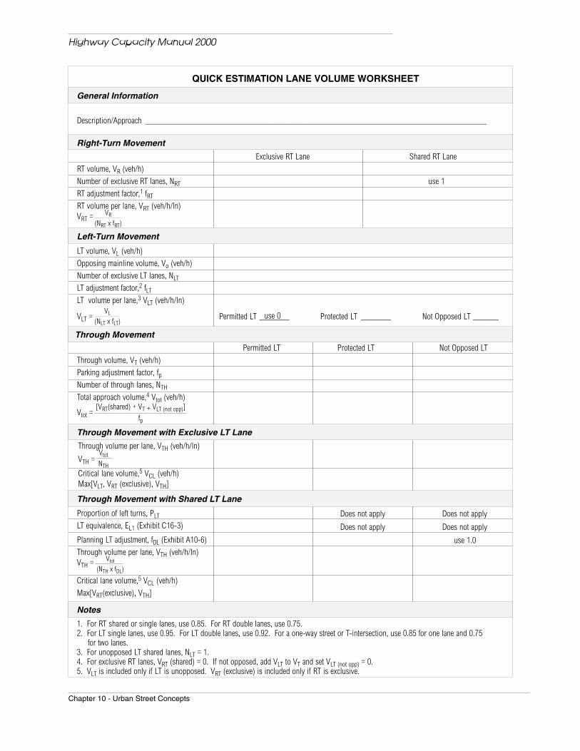
Chapter 10 - Urban Street Concepts
Highway Capacity Manual 2000
QUICK ESTIMATION LANE VOLUME WORKSHEET
Description/Approach ________________________________________________________________________________
Exclusive RT Lane Shared RT Lane
RT volume, VR (veh/h)
Number of exclusive RT lanes, NRT use 1
RT adjustment factor,1 fRT
RT volume per lane, VRT (veh/h/ln)VRT =
LT volume, VL (veh/h)
Opposing mainline volume, Vo (veh/h)
Number of exclusive LT lanes, NLT
LT adjustment factor,2 fLT
LT volume per lane,3 VLT (veh/h/ln)
VLT = Permitted LT _______ Protected LT _______ Not Opposed LT ______
Permitted LT Protected LT Not Opposed LT
Through volume, VT (veh/h)
Parking adjustment factor, fpNumber of through lanes, NTH
Total approach volume,4 Vtot (veh/h)
Vtot =
Through volume per lane, VTH (veh/h/ln)
VTH =
Critical lane volume,5 VCL (veh/h)Max[VLT, VRT (exclusive), VTH]
use 0
Does not apply Does not apply
Does not apply Does not apply
use 1.0
Proportion of left turns, PLT
LT equivalence, EL1 (Exhibit C16-3)
Planning LT adjustment, fDL (Exhibit A10-6)
Through volume per lane, VTH (veh/h/ln)VTH =
Critical lane volume,5 VCL (veh/h)
Max[VRT(exclusive), VTH]
1. For RT shared or single lanes, use 0.85. For RT double lanes, use 0.75.2. For LT single lanes, use 0.95. For LT double lanes, use 0.92. For a one-way street or T-intersection, use 0.85 for one lane and 0.75
for two lanes.3. For unopposed LT shared lanes, NLT = 1.4. For exclusive RT lanes, VRT (shared) = 0. If not opposed, add VLT to VT and set VLT (not opp) = 0.5. VLT is included only if LT is unopposed. VRT (exclusive) is included only if RT is exclusive.
General Information
Right-Turn Movement
Left-Turn Movement
Through Movement
Through Movement with Exclusive LT Lane
Through Movement with Shared LT Lane
Notes
Vtot
(NTH x fDL)
Vtot
NTH
VL
(NLT x fLT)
VR
(NRT x fRT)
[VRT(shared) + VT + VLT (not opp)]
fp

Chapter 10 - Urban Street Concepts
g = (C – L) + tL( )CVCS
g = (C – L) + tL( )CVCS
V/sg/C
X =
VX
c =
∑(d)(V)∑V
∑(dA)(VA)∑VA
dI =
LC
1 –( )(1700*PHF*fa)
CSXc =
L
1 –C = CS
RS
Selected plan (Exhibit A10-8) ________ Phase No. 1 Phase No. 2 Phase No. 3Movement codesCritical phase volume, CV (veh/h)Lost time/phase, tL (s)
Selected plan (Exhibit A10-8) ________ Phase No. 1 Phase No. 2 Phase No. 3Movement codesCritical phase volume, CV (veh/h)Lost time/phase, tL (s)
EB WB NB SB
Lane group
Lane group adjusted volume from lane volumeworksheet, V (veh/h)
Green ratio, g/C
Lane group saturation flow rate, s (veh/h)s = RS * number of lanes in lane group
v/c ratio, X
Lane group capacity, c (veh/h)
Progression adjustment factor, PF (Exhibit 16-12)
Uniform delay, d1 (s/veh) (Equation 16-11)
Incremental delay, d2 (s/veh) (Equation 16-12)
Initial queue delay, d3 (s/veh) (Appendix F, Ch. 16)
Delay, d = d1(PF) + d2 + d3 (s/veh)
Delay by approach, dA (s/veh)
Approach flow rate, VA (veh/h)
Intersection delay, dI (s/veh)
Description________________________________________________________________________________________
QUICK ESTIMATION CONTROL DELAY AND LOS WORKSHEET
General Information
East-West Phasing Plan
North-South Phasing Plan
Intersection Status Computation
Control Delay and LOS
Green Time Calculation
Notes
1. RS = 1530(PHF)(fa), where fa is area adjustment factor (0.90 for CBD and 1.0 for all others).
Critical sum, CS (veh/h) CS = ∑CVLost time/cycle, L (s) L = ∑ tLReference sum flow rate RS (veh/h)1
Cycle length, C (s)Cmin ≤ C ≤ CmaxC = Cmax when CS ≥ RSCritical v/c ratio, Xc
Intersection status (Exhibit A10-9)
East-West Phasing Phase No. 1 Phase No. 2 Phase No. 3
Green time, g (s)
North-South Phasing Phase No. 1 Phase No. 2 Phase No. 3
Green time, g (s)
Intersection LOS (Exhibit 16-2)
Highway Capacity Manual 2000