Cellular Automata Models

Maria ByrneAugust 10th 2005

VICBC1st Annual Workshop

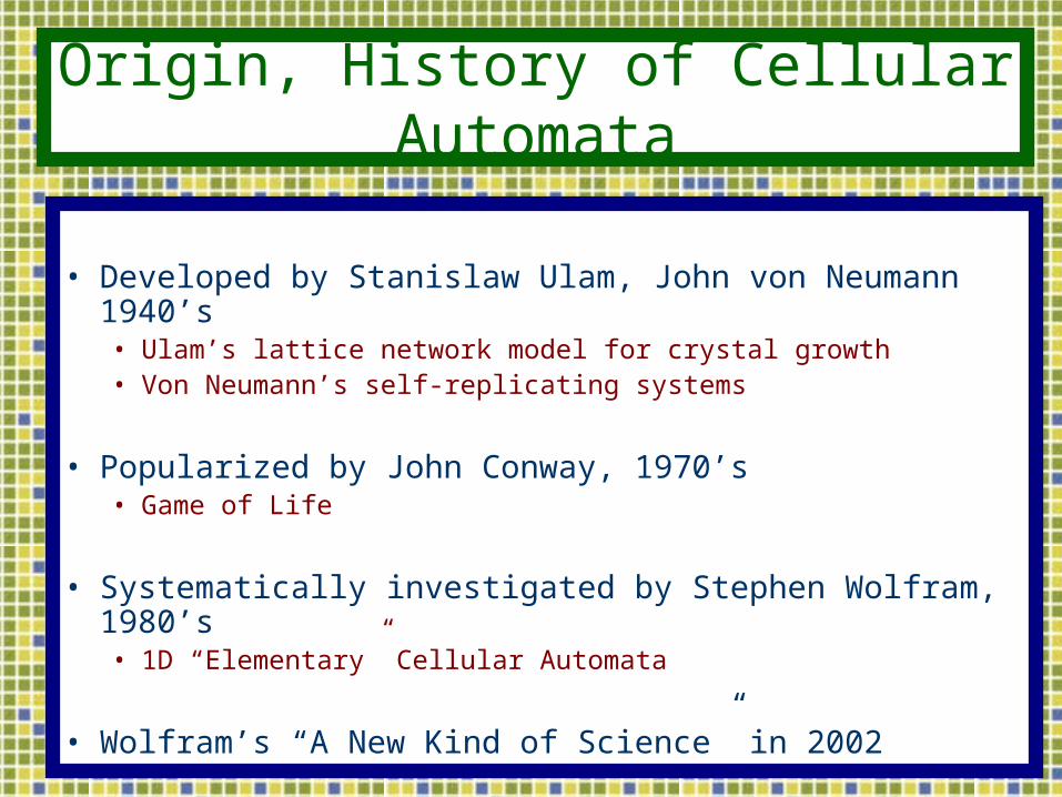
Origin, History of Cellular Automata

• Developed by Stanislaw Ulam, John von Neumann 1940’s• Ulam’s lattice network model for crystal growth• Von Neumann’s self-replicating systems

• Popularized by John Conway, 1970’s• Game of Life

• Systematically investigated by Stephen Wolfram, 1980’s• 1D “Elementary” Cellular Automata

• Wolfram’s “A New Kind of Science” in 2002

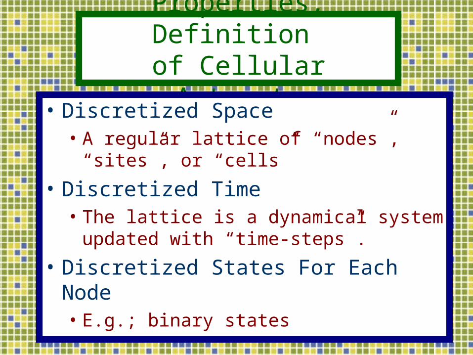
Properties, Definition of Cellular Automata

• Discretized Space • A regular lattice of “nodes”, “sites”, or “cells”

• Discretized Time • The lattice is a dynamical system updated

with “time-steps”.

• Discretized States For Each Node• E.g.; binary states

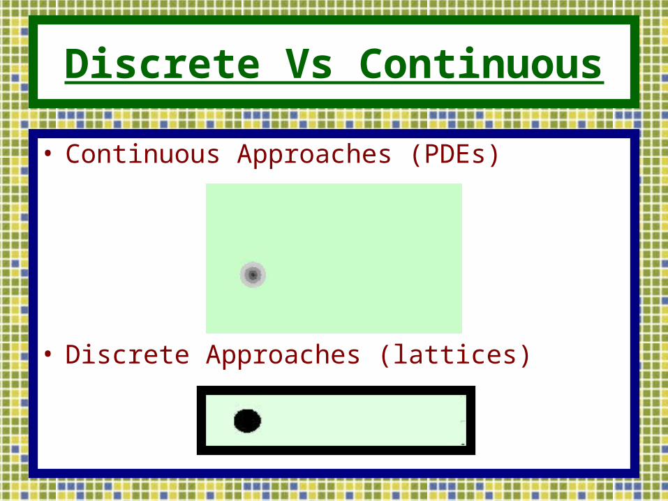
Discrete Vs Continuous

• Continuous Approaches (PDEs)

• Discrete Approaches (lattices)

Properties, Definition of Cellular Automata

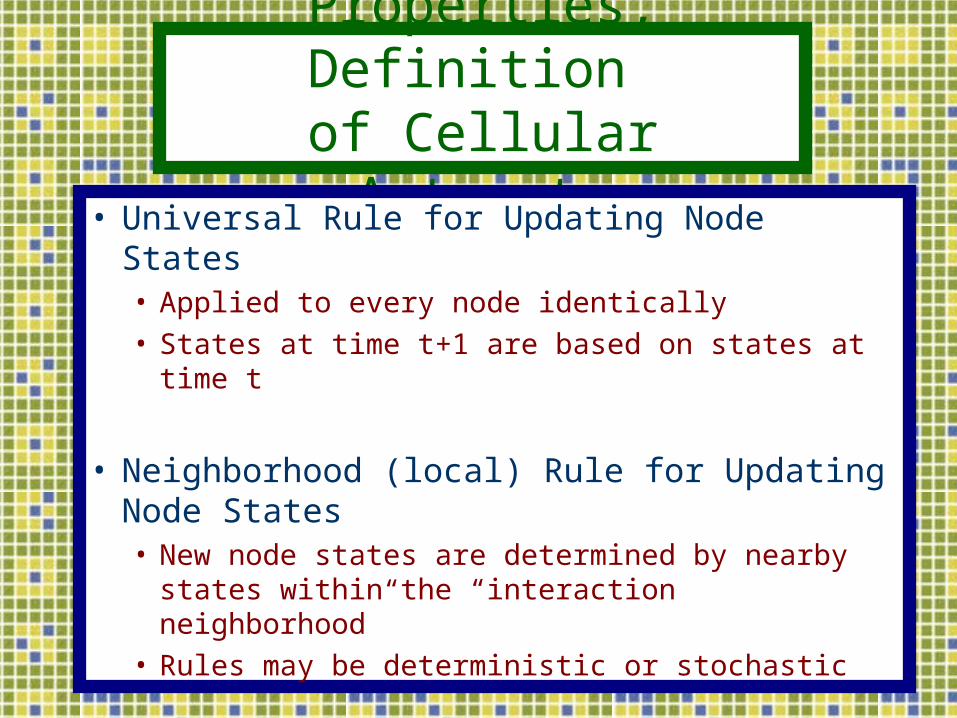
• Universal Rule for Updating Node States• Applied to every node identically• States at time t+1 are based on states at time t

• Neighborhood (local) Rule for Updating Node States• New node states are determined by nearby states

within the “interaction neighborhood”• Rules may be deterministic or stochastic

Example of an Elementary CA

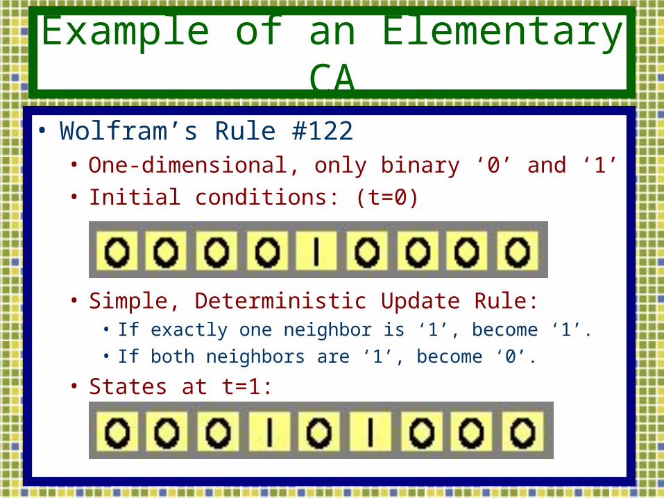
• Wolfram’s Rule #122• One-dimensional, only binary ‘0’ and ‘1’• Initial conditions: (t=0)

• Simple, Deterministic Update Rule:• If exactly one neighbor is ‘1’, become ‘1’.• If both neighbors are ‘1’, become ‘0’.

• States at t=1:

Example of an Elementary CA

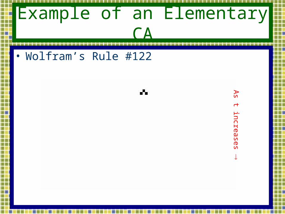
• Wolfram’s Rule #122A

s t increases

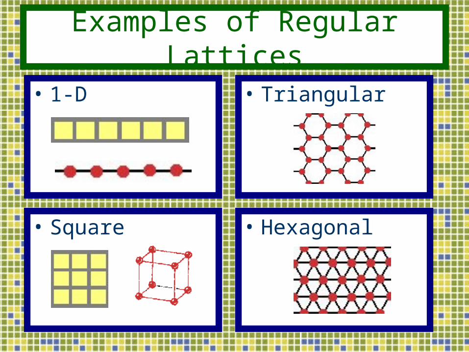
Examples of Regular Lattices

• 1-D

• Square

• Triangular

• Hexagonal

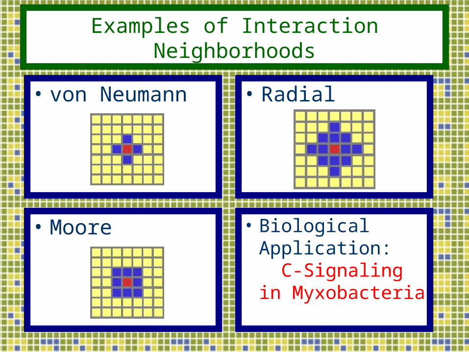
Examples of Interaction Neighborhoods

• von Neumann

• Moore

• Radial

• Biological Application: C-Signaling in Myxobacteria

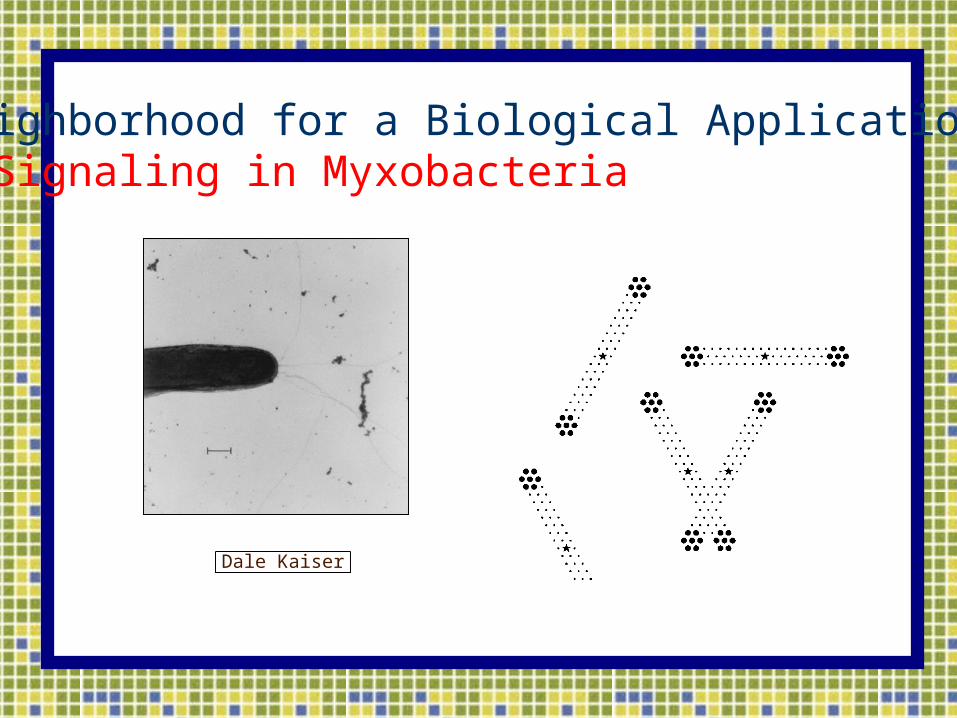
Dale Kaiser

Neighborhood for a Biological Application:C-Signaling in Myxobacteria

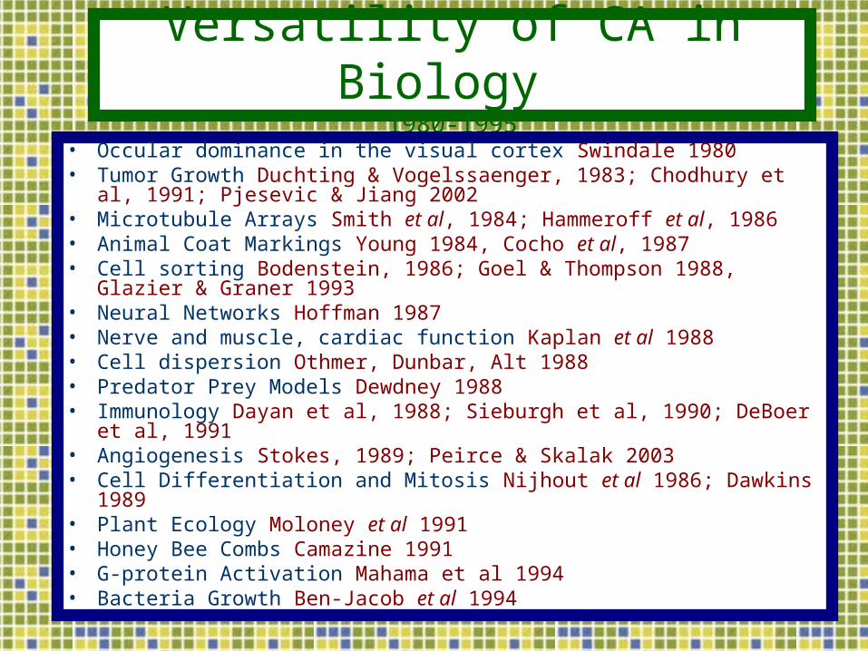
Versatility of CA in Biology 1980-1995

• Occular dominance in the visual cortex Swindale 1980• Tumor Growth Duchting & Vogelssaenger, 1983; Chodhury et al, 1991;

Pjesevic & Jiang 2002• Microtubule Arrays Smith et al, 1984; Hammeroff et al, 1986• Animal Coat Markings Young 1984, Cocho et al, 1987• Cell sorting Bodenstein, 1986; Goel & Thompson 1988, Glazier & Graner

1993• Neural Networks Hoffman 1987• Nerve and muscle, cardiac function Kaplan et al 1988• Cell dispersion Othmer, Dunbar, Alt 1988• Predator Prey Models Dewdney 1988• Immunology Dayan et al, 1988; Sieburgh et al, 1990; DeBoer et al, 1991• Angiogenesis Stokes, 1989; Peirce & Skalak 2003• Cell Differentiation and Mitosis Nijhout et al 1986; Dawkins 1989 • Plant Ecology Moloney et al 1991• Honey Bee Combs Camazine 1991• G-protein Activation Mahama et al 1994• Bacteria Growth Ben-Jacob et al 1994

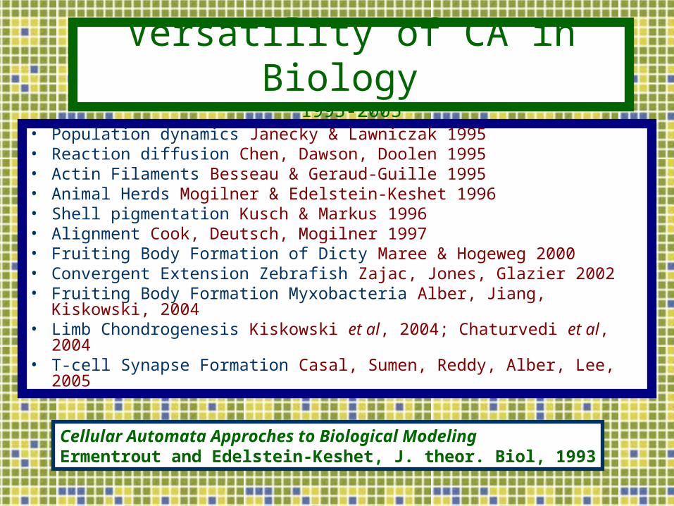
• Population dynamics Janecky & Lawniczak 1995• Reaction diffusion Chen, Dawson, Doolen 1995• Actin Filaments Besseau & Geraud-Guille 1995• Animal Herds Mogilner & Edelstein-Keshet 1996• Shell pigmentation Kusch & Markus 1996• Alignment Cook, Deutsch, Mogilner 1997• Fruiting Body Formation of Dicty Maree & Hogeweg 2000• Convergent Extension Zebrafish Zajac, Jones, Glazier 2002• Fruiting Body Formation Myxobacteria Alber, Jiang, Kiskowski, 2004• Limb Chondrogenesis Kiskowski et al, 2004; Chaturvedi et al, 2004• T-cell Synapse Formation Casal, Sumen, Reddy, Alber, Lee, 2005

Cellular Automata Approches to Biological ModelingErmentrout and Edelstein-Keshet, J. theor. Biol, 1993

Versatility of CA in Biology 1995-2005

Phototaxis during the Slug Stage of Dictyostelium discoideum: a Model StudyMarée, Panfilov and Hogeweg Proceedings of the Royal Society of London. Series B. Biological sciences 266 (1999) 1351-1360

Advantages of Cellular Automata

• Straight-forward implementation.• Local rules are intuitive and easy to modify.• Transversing length scales:

• Cells are a natural mesoscopic unit.• With modern computational power, 10^3-10^5

cells can be modeled on a PC.• Physical Mechanisms easily verified

• In silico response variables may be the same as for an in vivo experiment.

• Reflects intrinsic individuality of cells.• Unbounded complexity potential.

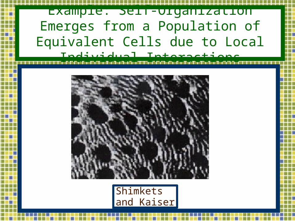
Example: Self-Organization Emerges from a Population of Equivalent Cells due to Local

Individual Interactions

Shimkets and Kaiser

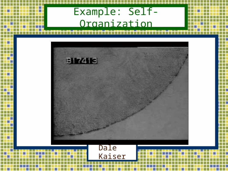
Example: Self-Organization

Dale Kaiser

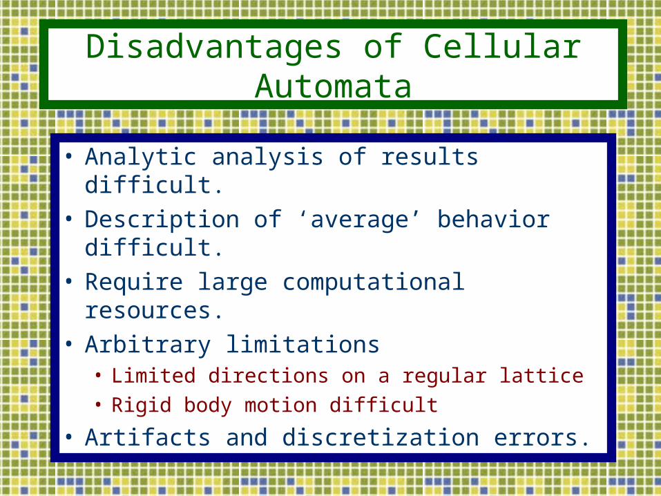
Disadvantages of Cellular Automata

• Analytic analysis of results difficult.• Description of ‘average’ behavior difficult.• Require large computational resources.• Arbitrary limitations

• Limited directions on a regular lattice• Rigid body motion difficult

• Artifacts and discretization errors.

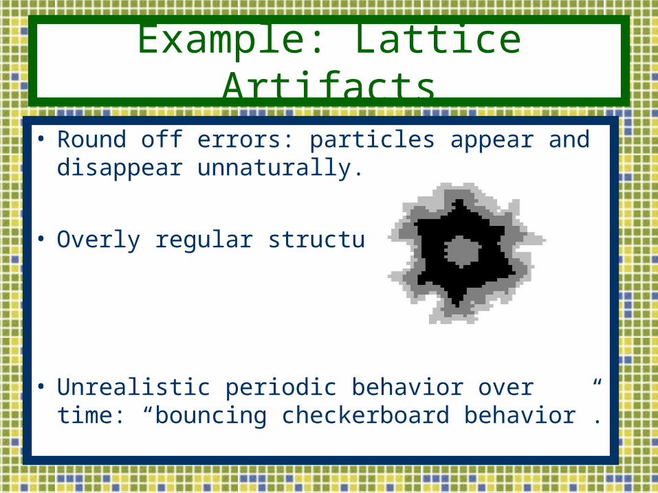
Example: Lattice Artifacts

• Round off errors: particles appear and disappear unnaturally.

• Overly regular structures.

• Unrealistic periodic behavior over time: “bouncing checkerboard behavior”.

Building a Cellular Automata:Diffusion

• Software..• Mathematica• C, C++• Fortran• Matlab

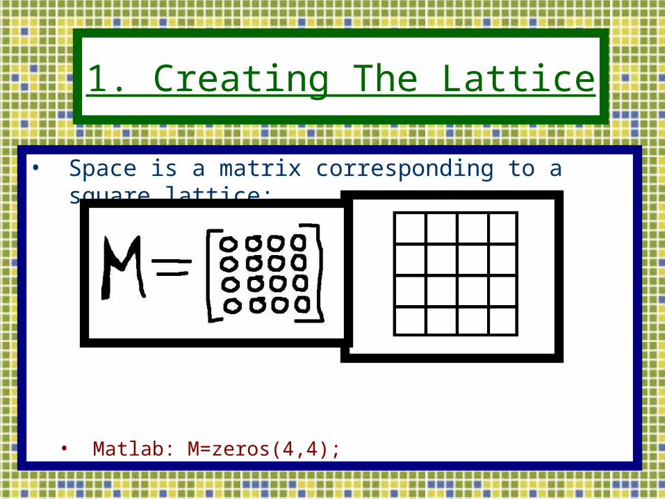
1. Creating The Lattice

• Space is a matrix corresponding to a square lattice:

• Matlab: M=zeros(4,4);

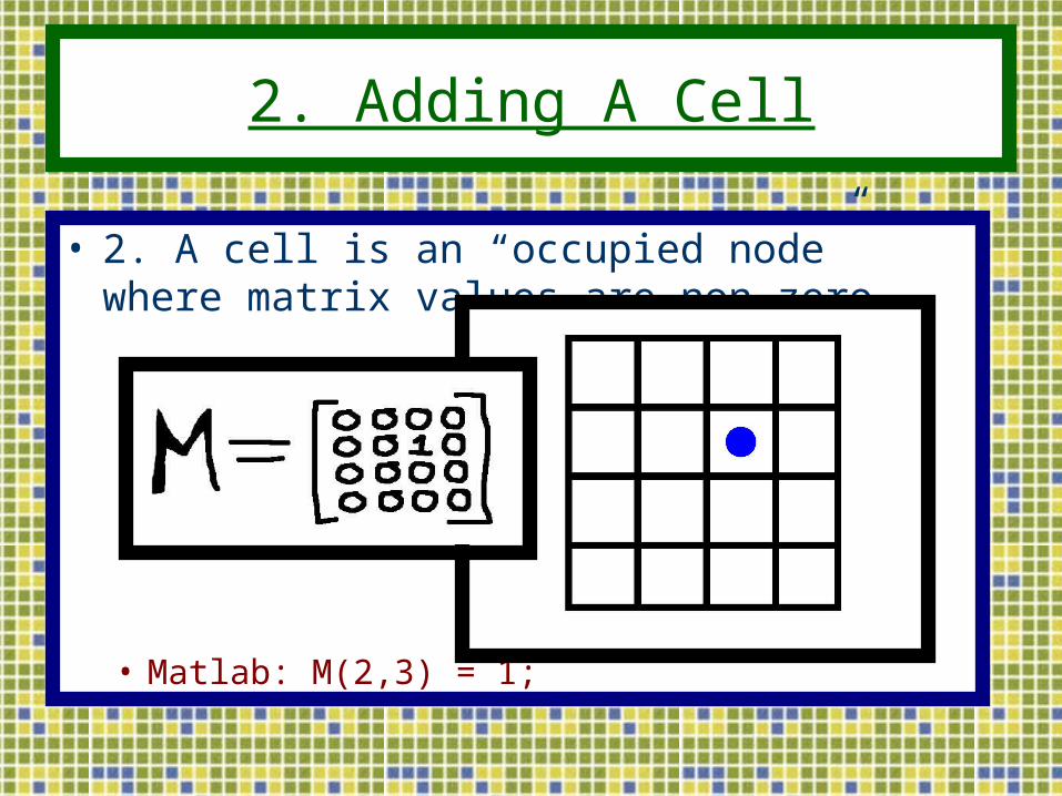
2. Adding A Cell

• 2. A cell is an “occupied node” where matrix values are non-zero.

• Matlab: M(2,3) = 1;

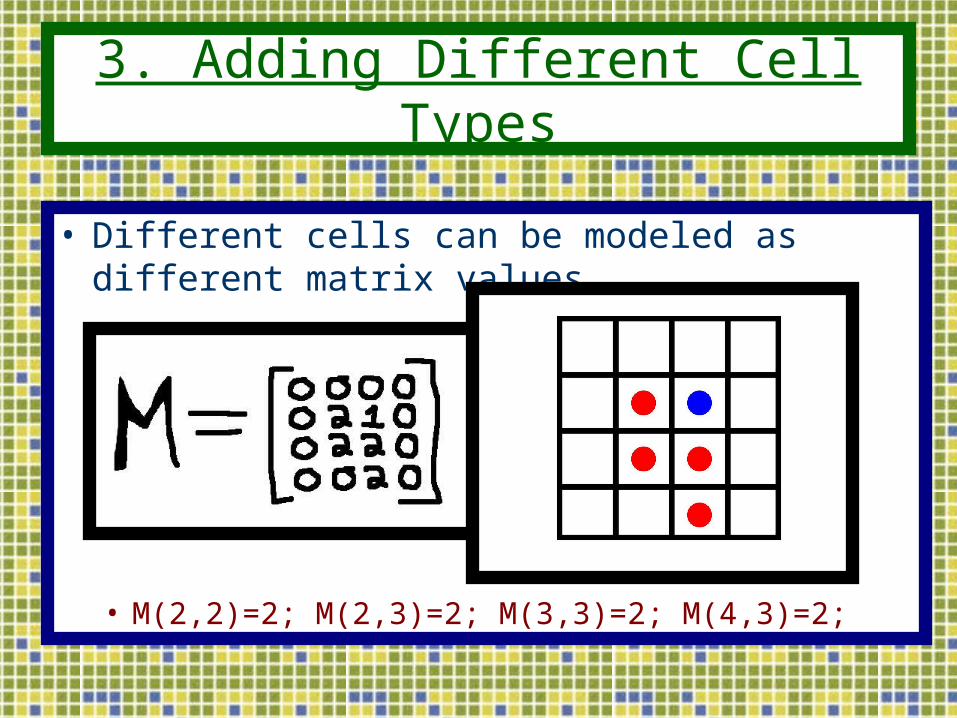
3. Adding Different Cell Types

• Different cells can be modeled as different matrix values.

• M(2,2)=2; M(2,3)=2; M(3,3)=2; M(4,3)=2;

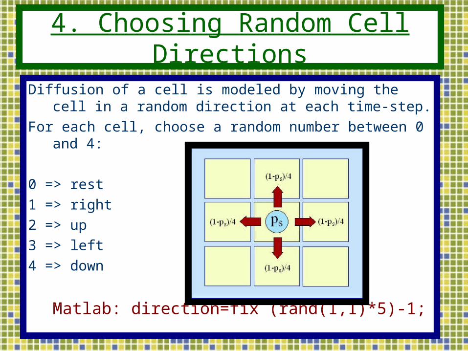
4. Choosing Random Cell Directions

Diffusion of a cell is modeled by moving the cell in a random direction at each time-step.

For each cell, choose a random number between 0 and 4:

0 => rest

1 => right

2 => up

3 => left

4 => down

Matlab: direction=fix (rand(1,1)*5)-1;

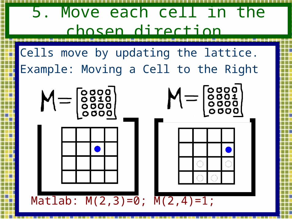
5. Move each cell in the chosen direction.

Cells move by updating the lattice.

Example: Moving a Cell to the Right

Matlab: M(2,3)=0; M(2,4)=1;

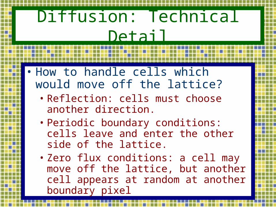
Diffusion: Technical Detail

• How to handle cells which would move off the lattice?• Reflection: cells must choose another

direction.• Periodic boundary conditions: cells leave

and enter the other side of the lattice.• Zero flux conditions: a cell may move off

the lattice, but another cell appears at random at another boundary pixel

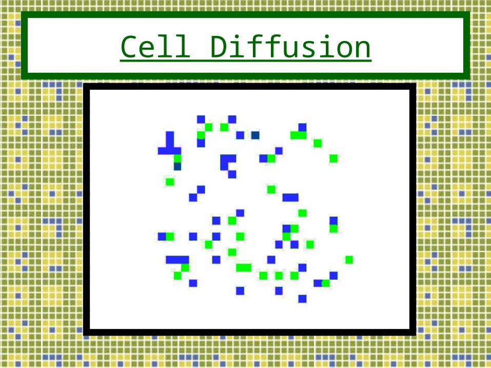
Cell Diffusion

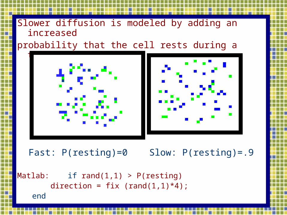
Slower diffusion is modeled by adding an increasedprobability that the cell rests during a timestep.

Fast: P(resting)=0 Slow: P(resting)=.9

Matlab: if rand(1,1) > P(resting) direction = fix (rand(1,1)*4); end

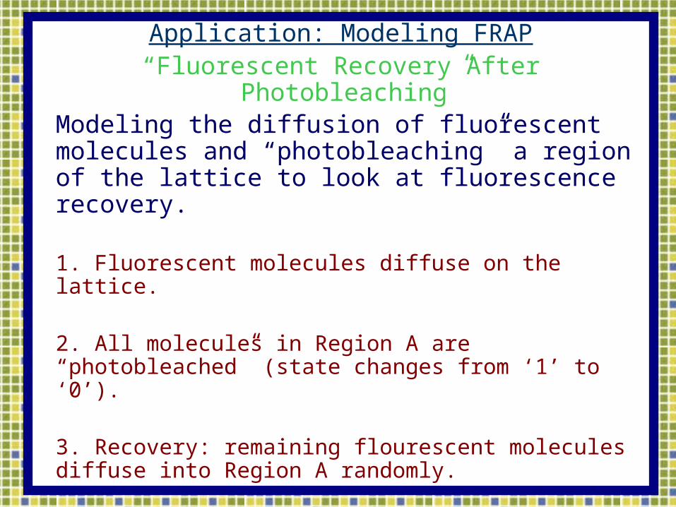
Application: Modeling FRAP“Fluorescent Recovery After Photobleaching”Modeling the diffusion of fluorescent molecules and “photobleaching” a region of the lattice to look at fluorescence recovery.

1. Fluorescent molecules diffuse on the lattice.

2. All molecules in Region A are “photobleached” (state changes from ‘1’ to ‘0’).

3. Recovery: remaining flourescent molecules diffuse into Region A randomly.

Application: Modeling FRAP

Modeling the diffusion of fluorescent molecules and “photobleaching” a region of the lattice to look at fluorescence recovery.

Building a Cellular Automata:Diffusion and Growth

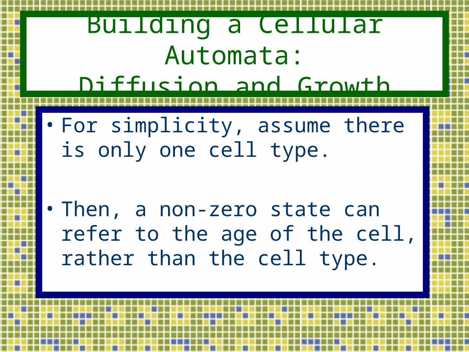
Building a Cellular Automata:Diffusion and Growth

• For simplicity, assume there is only one cell type.

• Then, a non-zero state can refer to the age of the cell, rather than the cell type.

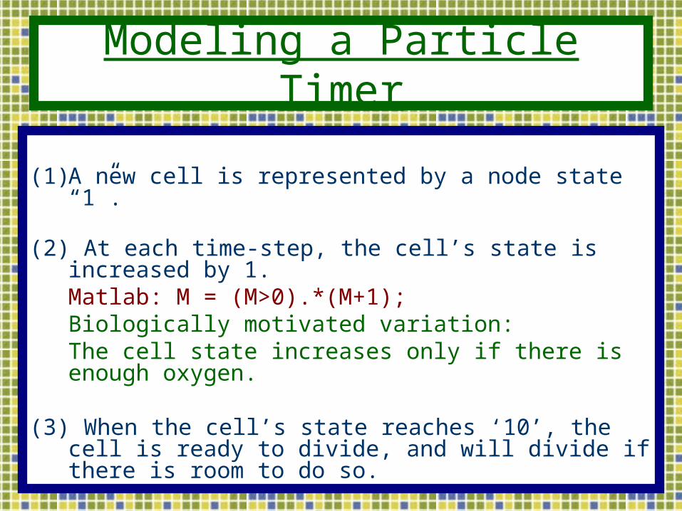
Modeling a Particle Timer

(1) A new cell is represented by a node state “1”.

(2) At each time-step, the cell’s state is increased by 1.Matlab: M = (M>0).*(M+1);Biologically motivated variation:The cell state increases only if there is enough oxygen.

(3) When the cell’s state reaches ‘10’, the cell is ready to divide, and will divide if there is room to do so.

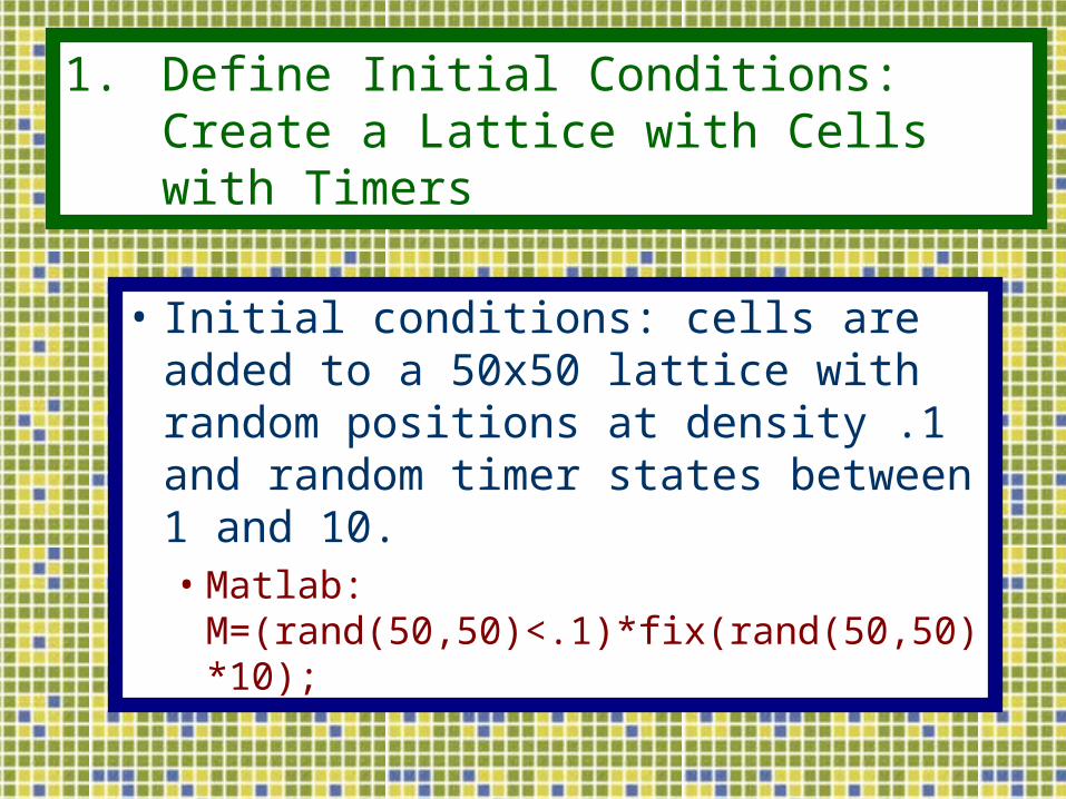
1. Define Initial Conditions:Create a Lattice with Cells with Timers

• Initial conditions: cells are added to a 50x50 lattice with random positions at density .1 and random timer states between 1 and 10.• Matlab:

M=(rand(50,50)<.1)*fix(rand(50,50)*10);

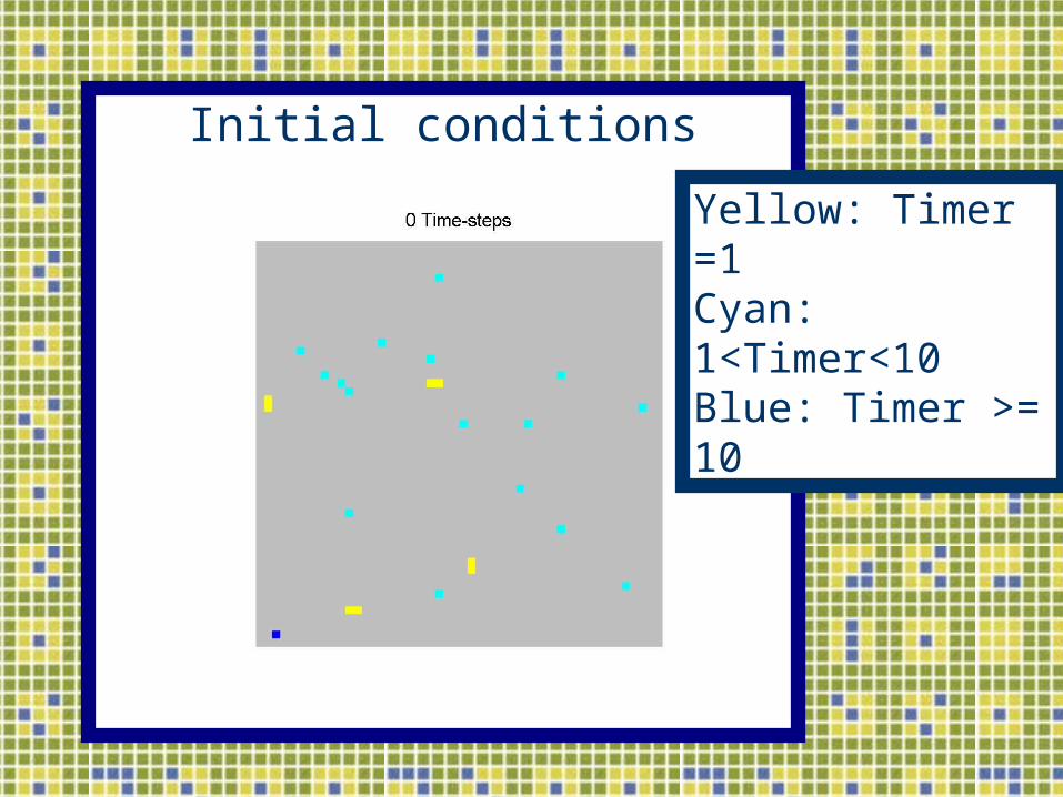
Initial conditions

Yellow: Timer =1Cyan: 1<Timer<10Blue: Timer >= 10

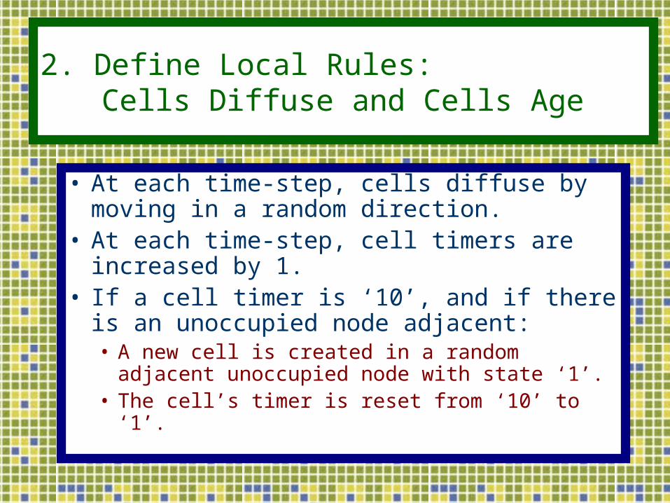
2. Define Local Rules:Cells Diffuse and Cells Age

• At each time-step, cells diffuse by moving in a random direction.

• At each time-step, cell timers are increased by 1.

• If a cell timer is ‘10’, and if there is an unoccupied node adjacent:• A new cell is created in a random adjacent

unoccupied node with state ‘1’.• The cell’s timer is reset from ‘10’ to ‘1’.

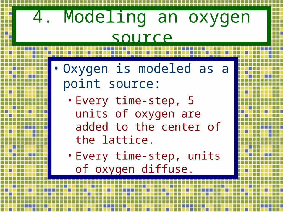
4. Modeling an oxygen source

• Oxygen is modeled as a point source:• Every time-step, 5 units of

oxygen are added to the center of the lattice.

• Every time-step, units of oxygen diffuse.

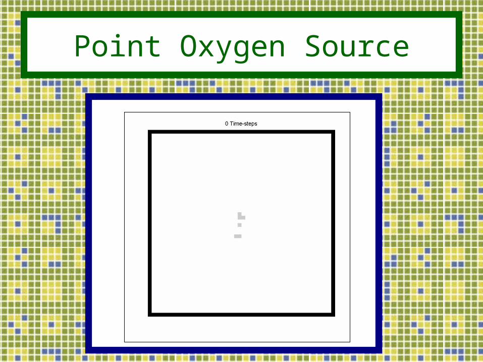
Point Oxygen Source

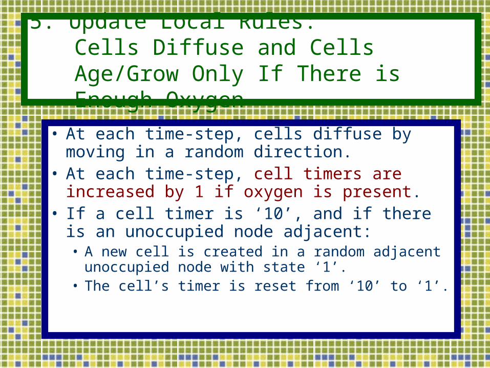
5. Update Local Rules:Cells Diffuse and Cells Age/Grow Only If There is Enough Oxygen

• At each time-step, cells diffuse by moving in a random direction.

• At each time-step, cell timers are increased by 1 if oxygen is present.

• If a cell timer is ‘10’, and if there is an unoccupied node adjacent:• A new cell is created in a random adjacent

unoccupied node with state ‘1’.• The cell’s timer is reset from ‘10’ to ‘1’.

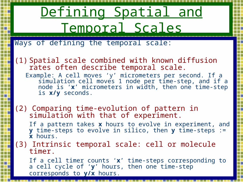
Defining Spatial and Temporal Scales

Ways of defining the temporal scale:

(1) Spatial scale combined with known diffusion rates often describe temporal scale.

Example: A cell moves ‘y’ micrometers per second. If a simulation cell moves 1 node per time-step, and if a node is ‘x’ micrometers in width, then one time-step is x/y seconds.

(2) Comparing time-evolution of pattern in simulation with that of experiment.If a pattern takes x hours to evolve in experiment, and y time-steps to evolve in silico, then y time-steps := x hours.

(3) Intrinsic temporal scale: cell or molecule timer. If a cell timer counts ‘x’ time-steps corresponding to a cell cycle of ‘y’ hours, then one time-step corresponds to y/x hours.

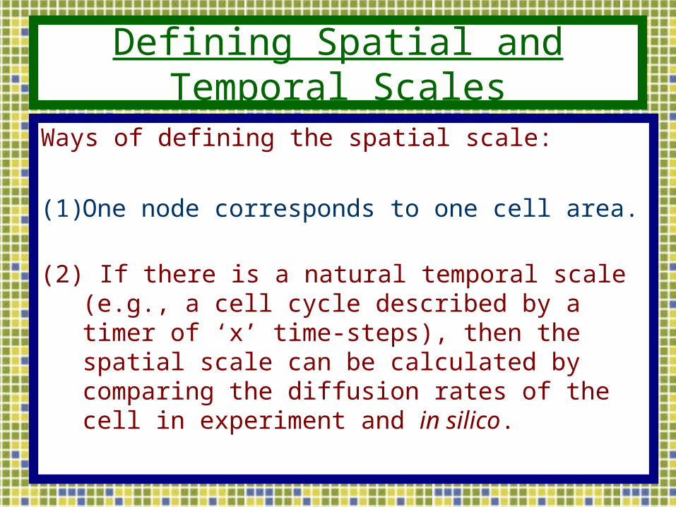
Defining Spatial and Temporal Scales

Ways of defining the spatial scale:

(1) One node corresponds to one cell area.

(2) If there is a natural temporal scale (e.g., a cell cycle described by a timer of ‘x’ time-steps), then the spatial scale can be calculated by comparing the diffusion rates of the cell in experiment and in silico.

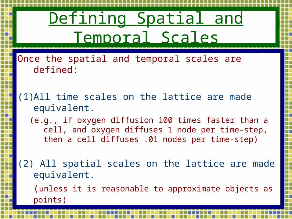
Defining Spatial and Temporal Scales

Once the spatial and temporal scales are defined:

(1) All time scales on the lattice are made equivalent. (e.g., if oxygen diffusion 100 times faster than a cell, and

oxygen diffuses 1 node per time-step, then a cell diffuses .01 nodes per time-step)

(2) All spatial scales on the lattice are made equivalent.

(unless it is reasonable to approximate objects as points)

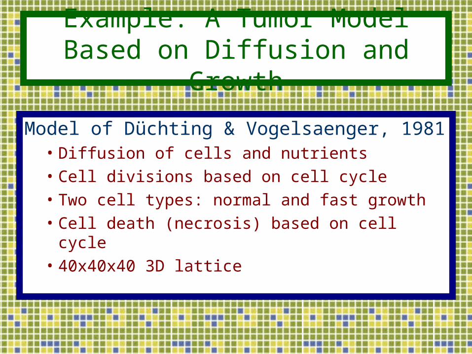
Example: A Tumor ModelBased on Diffusion and Growth

Model of Düchting & Vogelsaenger, 1981• Diffusion of cells and nutrients• Cell divisions based on cell cycle• Two cell types: normal and fast growth• Cell death (necrosis) based on cell cycle• 40x40x40 3D lattice

Types of CA Models

• Lattice Gases (LGCA)

• Bio-LGCA

• Pott’s Model

• Hybrid Models

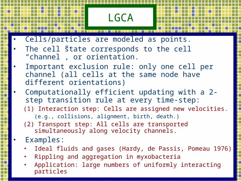
LGCA

• Cells/particles are modeled as points.• The cell state corresponds to the cell “channel”, or

orientation.• Important exclusion rule: only one cell per channel (all

cells at the same node have different orientations) • Computationally efficient updating with a 2-step transition

rule at every time-step:(1) Interaction step: Cells are assigned new velocities.

(e.g., collisions, alignment, birth, death.)

(2) Transport step: All cells are transported simultaneously along velocity channels.

• Examples:• Ideal fluids and gases (Hardy, de Passis, Pomeau 1976)• Rippling and aggregation in myxobacteria • Application: large numbers of uniformly interacting particles

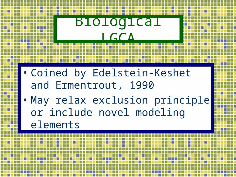
Biological LGCA

• Coined by Edelstein-Keshet and Ermentrout, 1990

• May relax exclusion principle or include novel modeling elements

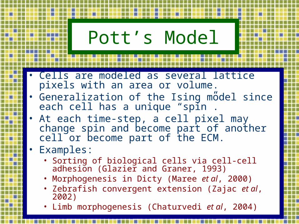
Pott’s Model

• Cells are modeled as several lattice pixels with an area or volume.

• Generalization of the Ising model since each cell has a unique “spin”.

• At each time-step, a cell pixel may change spin and become part of another cell or become part of the ECM.

• Examples:• Sorting of biological cells via cell-cell adhesion (Glazier and

Graner, 1993)• Morphogenesis in Dicty (Maree et al, 2000)• Zebrafish convergent extension (Zajac et al, 2002)• Limb morphogenesis (Chaturvedi et al, 2004)

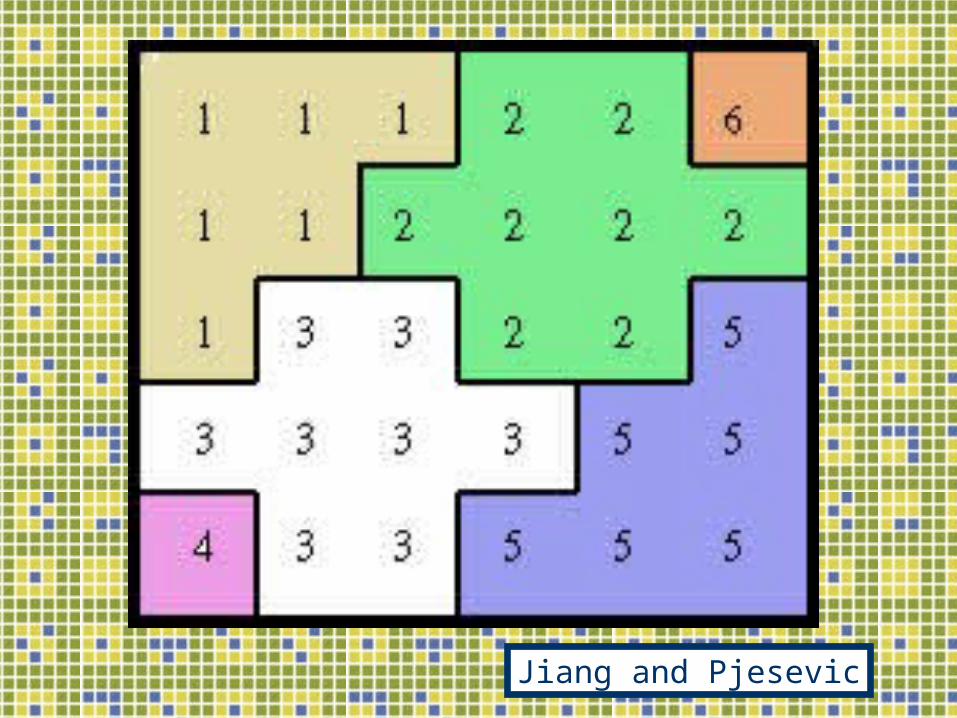
Jiang and Pjesevic

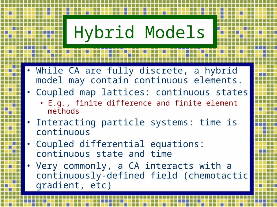
Hybrid Models

• While CA are fully discrete, a hybrid model may contain continuous elements.

• Coupled map lattices: continuous states• E.g., finite difference and finite element methods

• Interacting particle systems: time is continuous• Coupled differential equations: continuous state and

time• Very commonly, a CA interacts with a continuously-

defined field (chemotactic gradient, etc)

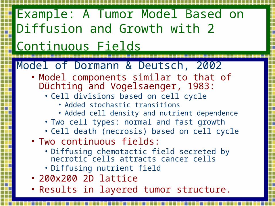
Example: A Tumor Model Based on Diffusion

and Growth with 2 Continuous Fields

Model of Dormann & Deutsch, 2002• Model components similar to that of Düchting and

Vogelsaenger, 1983:• Cell divisions based on cell cycle

• Added stochastic transitions• Added cell density and nutrient dependence

• Two cell types: normal and fast growth• Cell death (necrosis) based on cell cycle

• Two continuous fields: • Diffusing chemotactic field secreted by necrotic cells attracts

cancer cells• Diffusing nutrient field

• 200x200 2D lattice• Results in layered tumor structure.

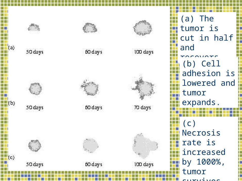
(a) The tumor is cut in half and recovers.

(b) Cell adhesion is lowered and tumor expands.

(c) Necrosis rate is increased by 1000%, tumor survives.

Thanks very much!

Cellular Automata or MATLAB questions?

abyrne@math.vanderbilt.edu

Excellent CA tutorial:

PhD thesis of Sabine Dormann,

“Pattern Formation in CA models”