Polyhedral Combinatorics

Carlo Mannino

(from Geir Dahl and Carlo Mannino notes)

University of Oslo, INF-MAT5360 - Autumn 2010 (Mathematical optimization)

Combinatorial Optimization Problem

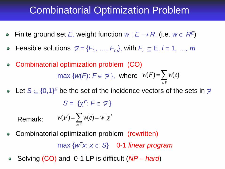
Finite ground set E, weight function w : E R. (i.e. w RE)

Feasible solutions F = {F1, …, Fm}, with Fi E, i = 1, …, m

Combinatorial optimization problem (CO)

max {w(F): F F }, where

Let S {0,1}E be the set of the incidence vectors of the sets in F

S = {F: F F }

Combinatorial optimization problem (rewritten)

max {wTx: x S} 0-1 linear program

Solving (CO) and 0-1 LP is difficult (NP – hard)

Fe

ewFw )()(

FT

Fe

wewFw

)()(Remark:

Example: project selection

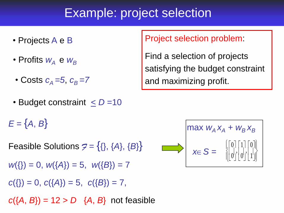
• Projects A e B

• Profits wA e wB

• Budget constraint < D =10

• Costs cA =5, cB =7

xS =

1

0 ,

0

1 ,

0

0

max wA xA + wB xB

Project selection problem:

Find a selection of projects

satisfying the budget constraint

and maximizing profit.

E = {A, B}

Feasible Solutions F = {{}, {A}, {B}}

w({}) = 0, w({A}) = 5, w({B}) = 7

c({}) = 0, c({A}) = 5, c({B}) = 7,

c({A, B}) = 12 > D {A, B} not feasible

From CO to LP

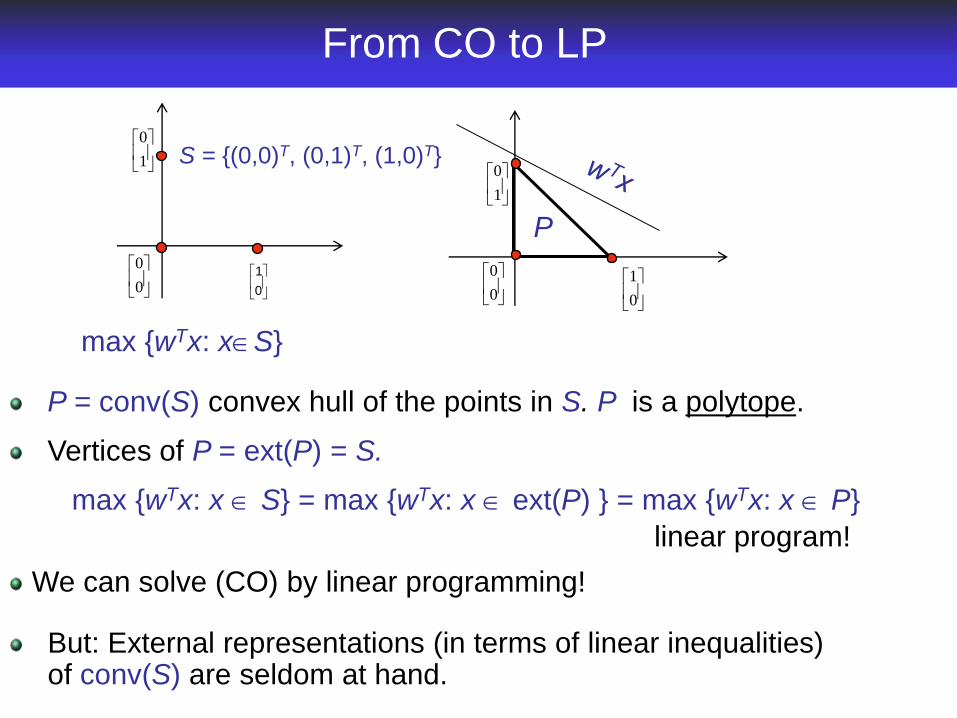
max {wTx: xS}

P = conv(S) convex hull of the points in S. P is a polytope.

Vertices of P = ext(P) = S.

max {wTx: x S} = max {wTx: x ext(P) } = max {wTx: x P}

S = {(0,0)T, (0,1)T, (1,0)T}

0

1

0

0

1

0

0

1

0

0

1

0

linear program!

P

We can solve (CO) by linear programming!

But: External representations (in terms of linear inequalities) of conv(S) are seldom at hand.

The maximum weight forest

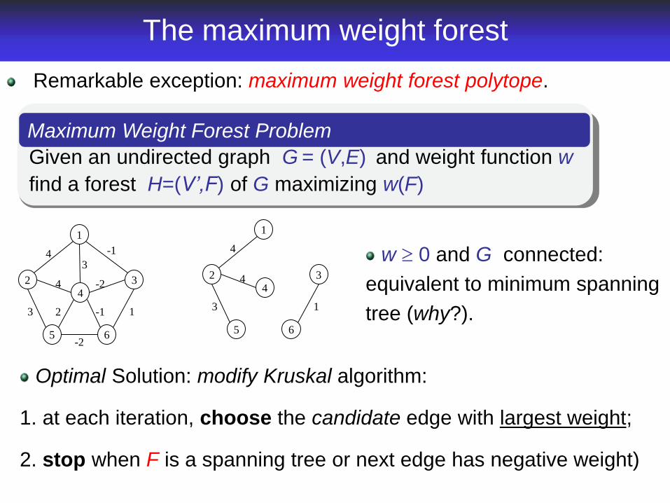
Remarkable exception: maximum weight forest polytope.

w 0 and G connected:

equivalent to minimum spanning

tree (why?).

Given an undirected graph G = (V,E) and weight function w

find a forest H=(V’,F) of G maximizing w(F)

Maximum Weight Forest Problem

2

65

3

1

3

-2

4

34 -1

1

4-2

-12

2

65

3

1

3

4

4

1

4

Optimal Solution: modify Kruskal algorithm:

1. at each iteration, choose the candidate edge with largest weight;

2. stop when F is a spanning tree or next edge has negative weight)

Incidence vectors of forests

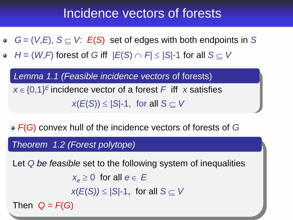
G = (V,E), S V: E(S) set of edges with both endpoints in S

H = (W,F) forest of G iff |E(S) F| |S|-1 for all S V

F(G) convex hull of the incidence vectors of forests of G

x {0,1}E incidence vector of a forest F iff x satisfies

x(E(S)) |S|-1, for all S V

Lemma 1.1 (Feasible incidence vectors of forests)

Let Q be feasible set to the following system of inequalities

xe 0 for all e E

x(E(S)) |S|-1, for all S V

Then Q = F(G)

Theorem 1.2 (Forest polytope)

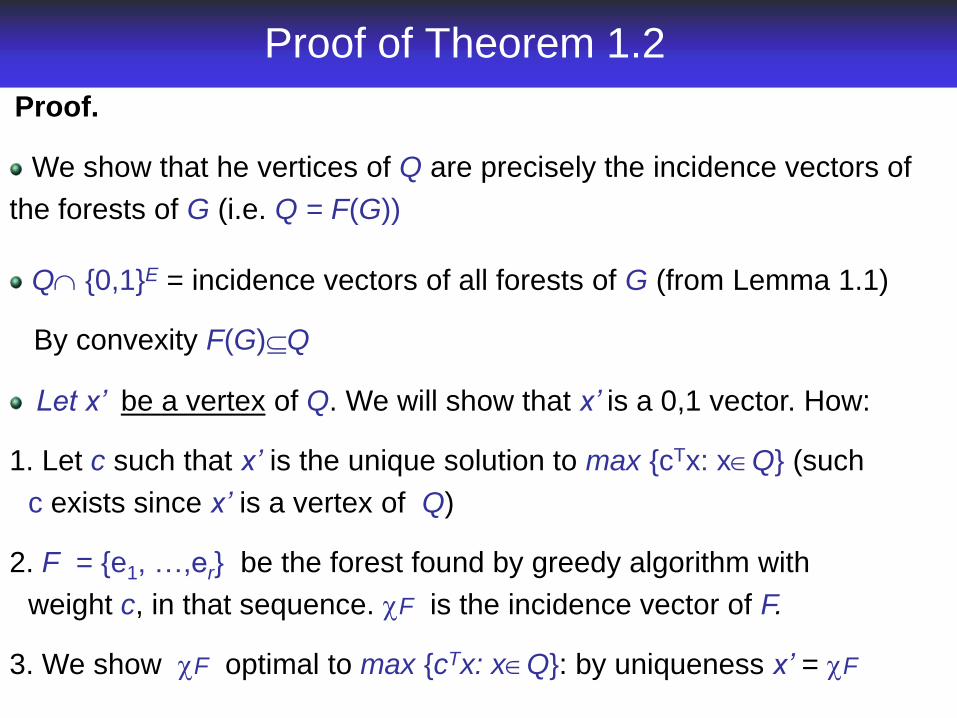
Proof of Theorem 1.2

Q {0,1}E = incidence vectors of all forests of G (from Lemma 1.1)

By convexity F(G)Q

Proof.

Let x’ be a vertex of Q. We will show that x’ is a 0,1 vector. How:

1. Let c such that x’ is the unique solution to max {cTx: xQ} (such

c exists since x’ is a vertex of Q)

2. F = {e1, …,er} be the forest found by greedy algorithm with

weight c, in that sequence. F is the incidence vector of F.

3. We show F optimal to max {cTx: xQ}: by uniqueness x’ = F

We show that he vertices of Q are precisely the incidence vectors of

the forests of G (i.e. Q = F(G))

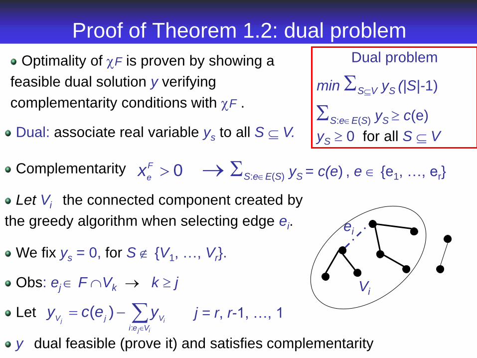
Proof of Theorem 1.2: dual problem

Dual: associate real variable ys to all S V.

y dual feasible (prove it) and satisfies complementarity

Dual problem

min SV yS (|S|-1)

S:eE(S) yS c(e)

yS 0 for all S V

ei

Vi

Optimality of F is proven by showing a

feasible dual solution y verifying

complementarity conditions with F .

Complementarity 0F

ex S:eE(S) yS = c(e) , e {e1, …, er}

We fix ys = 0, for S {V1, …, Vr}.

Obs: ej F Vk k j

Let

ij

ij

Vei

VjVyecy

:

)( j = r, r-1, …, 1

Let Vi the connected component created by

the greedy algorithm when selecting edge ei.

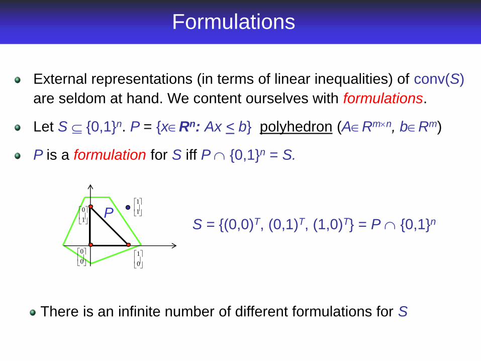
Formulations

External representations (in terms of linear inequalities) of conv(S)

are seldom at hand. We content ourselves with formulations.

Let S {0,1}n. P = {xRn: Ax < b} polyhedron (ARmn, bRm)

P is a formulation for S iff P {0,1}n = S.

1

1

0

1

0

0

1

0 PS = {(0,0)T, (0,1)T, (1,0)T} = P {0,1}n

There is an infinite number of different formulations for S

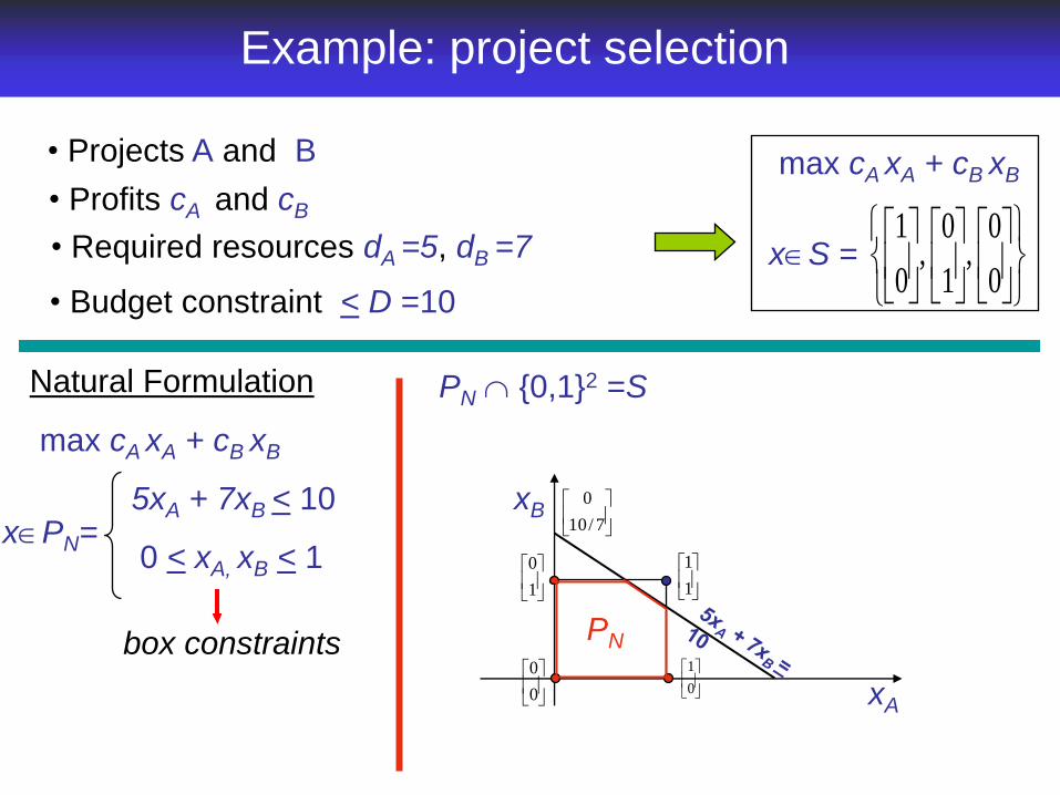
Example: project selection

• Projects A and B

• Profits cA and cB

• Budget constraint < D =10

• Required resources dA =5, dB =7 xS =

0

0 ,

1

0 ,

0

1

max cA xA + cB xB

PN {0,1}2 =S

box constraints

max cA xA + cB xB

xPN=

Natural Formulation

xA

xB

0

1

1

0

0

0

1

1

7/10

0

PN

0 < xA, xB < 1

5xA + 7xB < 10

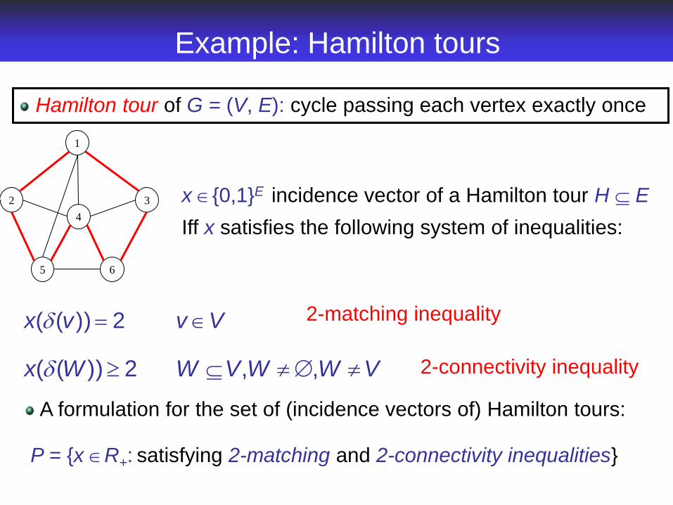
Example: Hamilton tours

Hamilton tour of G = (V, E): cycle passing each vertex exactly once

2

65

3

1

4

x {0,1}E incidence vector of a Hamilton tour H E

Iff x satisfies the following system of inequalities:

Vvvx 2))((

P = {x R+: satisfying 2-matching and 2-connectivity inequalities}

2-matching inequality

2-connectivity inequality VWWVWWx ,, 2))((

A formulation for the set of (incidence vectors of) Hamilton tours:

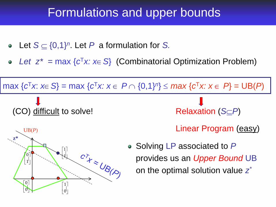
Formulations and upper bounds

Let S {0,1}n. Let P a formulation for S.

Let z* = max {cTx: xS} (Combinatorial Optimization Problem)

max {cTx: xS} = max {cTx: x P {0,1}n} max {cTx: x P} = UB(P)

UB(P)

z*

1

1

0

1

0

0

1

0

Relaxation (SP)

Linear Program (easy)

(CO) difficult to solve!

Solving LP associated to P

provides us an Upper Bound UB

on the optimal solution value z*

Formulations and certificates

max {cTx: x S}PL01:

UB(P) max {cTx: x S} = z*

• Computing z* is (in general) difficult

• Computing UB(P) is easy (LP program)

• If we know a feasible solution x S (with z =cTx lower bound)

then UB(P) provides a quality certificate for x .

UB(P)

z°

z* “gap”

UB(P)

z*

1

1

0

1

0

0

1

0

gap

z°

x°

cTx increasing

No “gap” x° optimal to PL01

(with S {0,1}n)

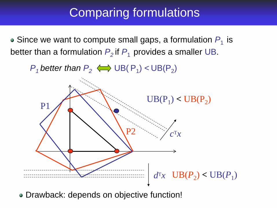
Comparing formulations

Since we want to compute small gaps, a formulation P1 is

better than a formulation P2 if P1 provides a smaller UB.

UB(P1) < UB(P2)P1

P2 cTx

dTx UB(P2) < UB(P1)

P1 better than P2 UB( P1) < UB(P2)

Drawback: depends on objective function!

Comparing formulations

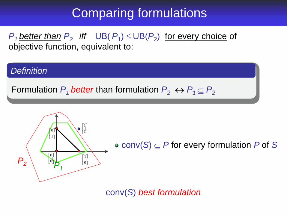
P1 better than P2 iff UB( P1) UB(P2) for every choice of

objective function, equivalent to:

Formulation P1 better than formulation P2 P1 P2

Definition

1

1

0

1

0

0

1

0

P2 P1

conv(S) P for every formulation P of S

conv(S) best formulation

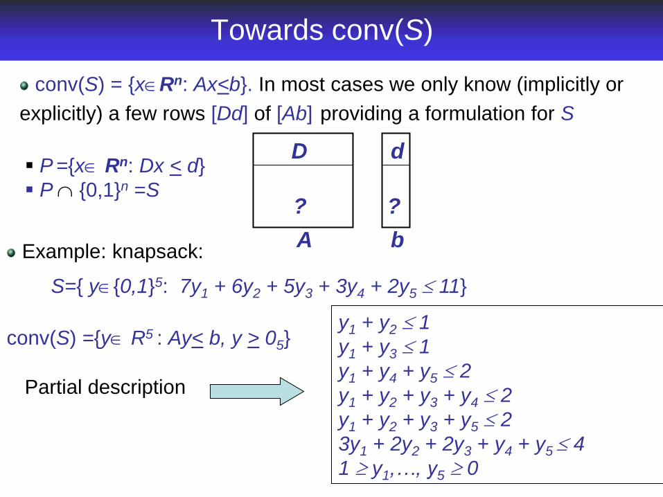
Towards conv(S)

conv(S) = {xRn: Ax<b}. In most cases we only know (implicitly or

explicitly) a few rows [Dd] of [Ab] providing a formulation for S

P ={x Rn: Dx < d}

P {0,1}n =S

A

D d

? ?

b

S={ y{0,1}5: 7y1 + 6y2 + 5y3 + 3y4 + 2y5 11}

conv(S) ={y R5 : Ay< b, y > 05}y1 + y2 1

y1 + y3 1

y1 + y4 + y5 2

y1 + y2 + y3 + y4 2

y1 + y2 + y3 + y5 2

3y1 + 2y2 + 2y3 + y4 + y5 4

1 y1,…, y5 0

Partial description

Example: knapsack:

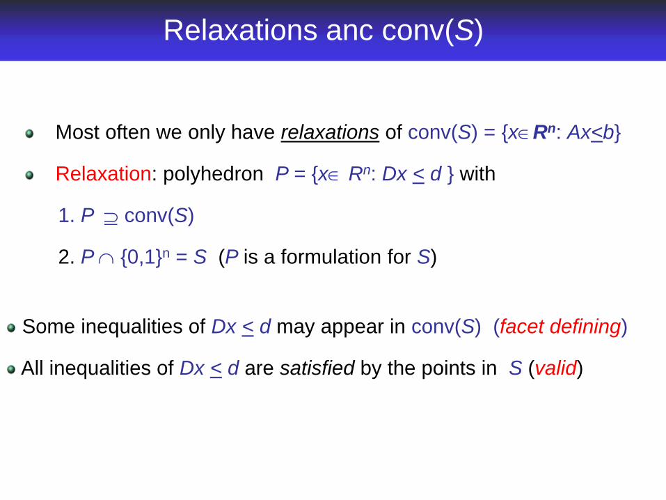
Relaxations anc conv(S)

Most often we only have relaxations of conv(S) = {xRn: Ax<b}

Relaxation: polyhedron P = {x Rn: Dx < d } with

1. P conv(S)

2. P {0,1}n = S (P is a formulation for S)

Some inequalities of Dx < d may appear in conv(S) (facet defining)

All inequalities of Dx < d are satisfied by the points in S (valid)

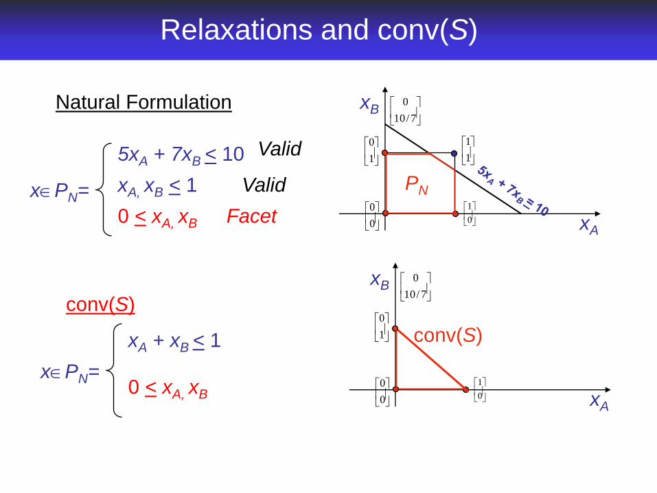
Relaxations and conv(S)

Facet

xPN=

Natural Formulation

xA

xB

0

1

1

0

0

0

1

1

7/10

0

PNxA, xB < 1

5xA + 7xB < 10

0 < xA, xB

Valid

Valid

xA

xB

0

1

1

0

0

0

7/10

0

conv(S)

xPN=

conv(S)

xA + xB < 1

0 < xA, xB

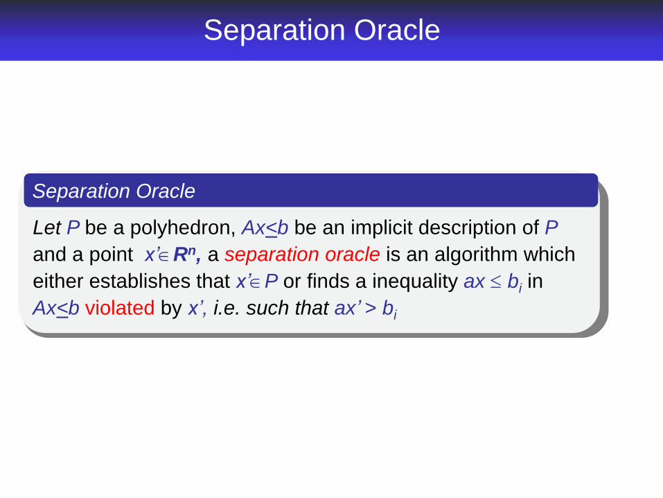
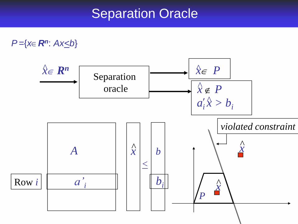
Separation Oracle

Let P be a polyhedron, Ax<b be an implicit description of P

and a point x’Rn, a separation oracle is an algorithm which

either establishes that x’P or finds a inequality ax bi in

Ax<b violated by x’, i.e. such that ax’ > bi

Separation Oracle

Separation Oracle

^ai x > bi

a’i Row i bi

x̂ PSeparation

oracle

x Rn^

x̂

x^

x̂ P

P ={xRn: Ax<b}

A x^

<

b

P

violated constraint

Separation for Maximum Weight Forest

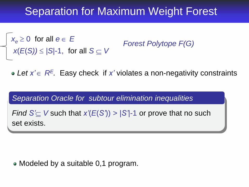
Find S’ V such that x’(E(S’)) > |S’|-1 or prove that no such

set exists.

Separation Oracle for subtour elimination inequalities

xe 0 for all e E

x(E(S)) |S|-1, for all S VForest Polytope F(G)

Let x’ RE. Easy check if x’ violates a non-negativity constraints

Modeled by a suitable 0,1 program.

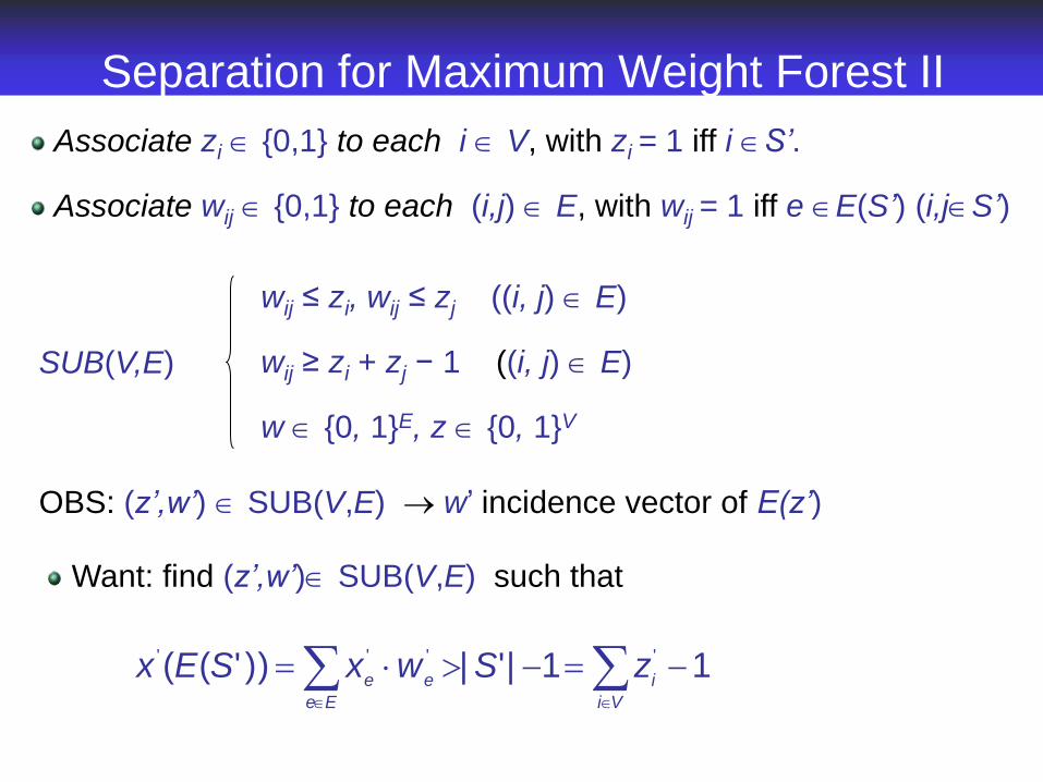
Separation for Maximum Weight Forest II

Associate zi {0,1} to each i V, with zi = 1 iff i S’.

Associate wij {0,1} to each (i,j) E, with wij = 1 iff e E(S’) (i,jS’)

wij ≤ zi, wij ≤ zj ((i, j) E)

wij ≥ zi + zj − 1 ((i, j) E)

w {0, 1}E, z {0, 1}V

SUB(V,E)

Want: find (z’,w’) SUB(V,E) such that

OBS: (z’,w’) SUB(V,E) w’ incidence vector of E(z’)

11|'|))'(( '''' Vi

ie

Ee

ezSwxSEx

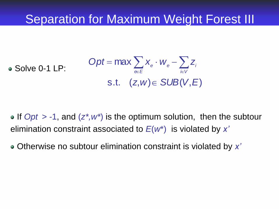
Separation for Maximum Weight Forest III

),(),( s.t.

max

EVSUBwz

zwxOptVi

ie

Ee

e

Solve 0-1 LP:

If Opt > -1, and (z*,w*) is the optimum solution, then the subtour

elimination constraint associated to E(w*) is violated by x’

Otherwise no subtour elimination constraint is violated by x’

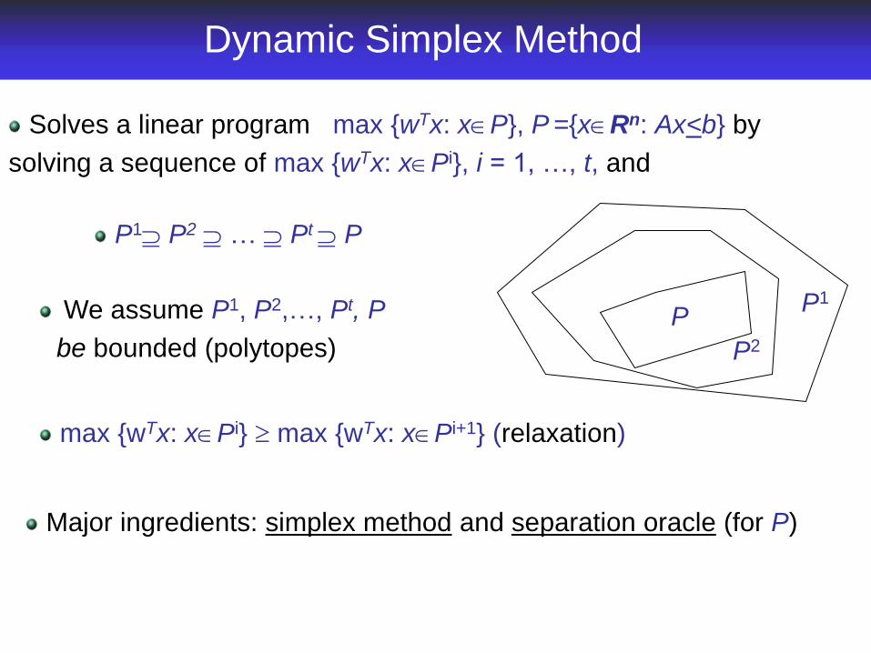
Dynamic Simplex Method

Solves a linear program max {wTx: xP}, P ={xRn: Ax<b} by

solving a sequence of max {wTx: xPi}, i = 1, …, t, and

max {wTx: xPi} max {wTx: xPi+1} (relaxation)

We assume P1, P2,…, Pt, P

be bounded (polytopes)

P1

P2

P

P1 P2 … Pt P

Major ingredients: simplex method and separation oracle (for P)

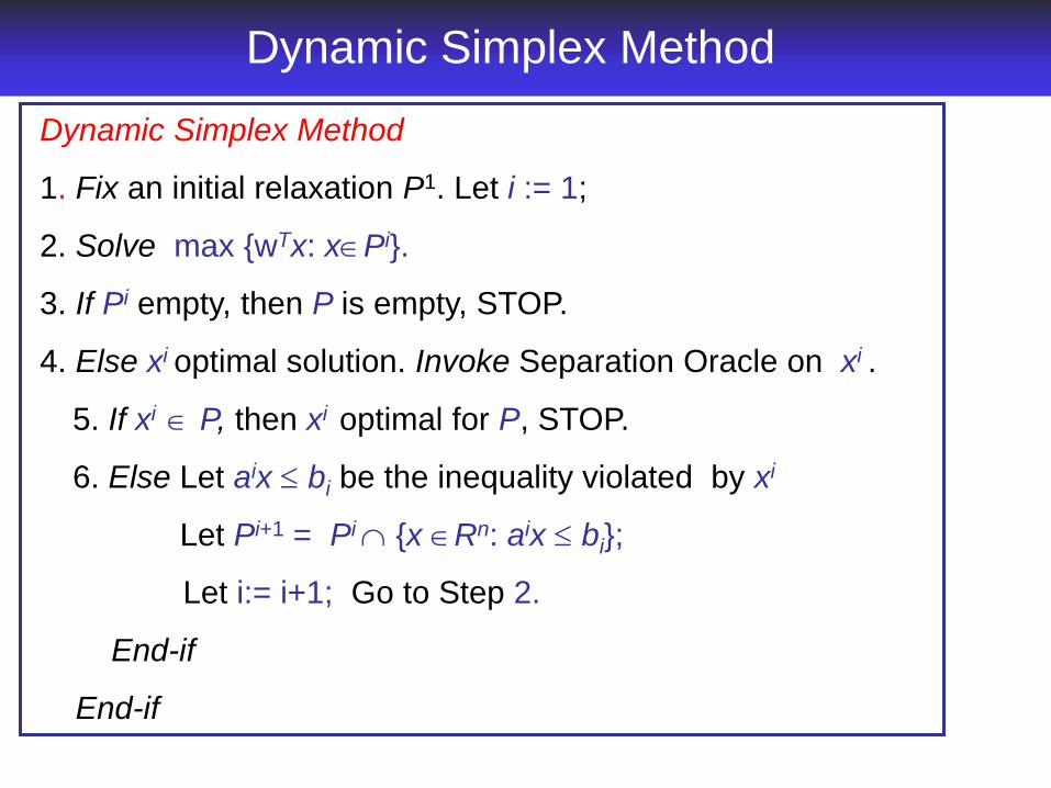
Dynamic Simplex Method

Dynamic Simplex Method

1. Fix an initial relaxation P1. Let i := 1;

2. Solve max {wTx: xPi}.

3. If Pi empty, then P is empty, STOP.

4. Else xi optimal solution. Invoke Separation Oracle on xi .

5. If xi P, then xi optimal for P, STOP.

6. Else Let aix bi be the inequality violated by xi

Let Pi+1 = Pi {x Rn: aix bi};

Let i:= i+1; Go to Step 2.

End-if

End-if

Exercises

Prove Lemma 1.1

Show that the Maximum Weight Forest Problem in a connected

graph with non-negative edge weights reduces to the minimum

spanning tree problem.

Show formally that the incidence vectors of Hamilton tour are

precisely the 0,1 vectors satisfying 2-matching and 2-connectivity

constraints.

Show formally that the dual solution in the proof of Theorem 2.1

is feasible.

If we apply the dynamic simplex method to the Maximum Weight

Forest Problem, then the last solution is a 0,1 solution. Why?