Cardiff Economics Working Papers

Working Paper No. E2014/20

The role of Fiscal policy in Britain’s Great Inflation

Jingwen Fan, Patrick Minford and Zhirong Ou

October 2014

Cardiff Business School

Aberconway Building

Colum Drive

Cardiff CF10 3EU

United Kingdom

t: +44 (0)29 2087 4000

f: +44 (0)29 2087 4419

business.cardiff.ac.uk

This working paper is produced for discussion purpose only. These working papers are expected to be

publishedin due course, in revised form, and should not be quoted or cited without the author’s written

permission.

Cardiff Economics Working Papers are available online from:

econpapers.repec.org/paper/cdfwpaper/ and

business.cardiff.ac.uk/research/academic-sections/economics/working-papers

Enquiries: EconWP@cardiff.ac.uk

The role of �scal policy in Britain�s Great In�ation�

Jingwen Fan

(Nottingham Trent University)

Patrick Minford

(Cardi¤ University and CEPR)

Zhirong Ouy

(Cardi¤ University)

Abstract

We investigate whether the Fiscal Theory of the Price Level (FTPL) can explain UK in�ation in

the 1970s. We confront the identi�cation problem involved by setting up the FTPL as a structural

model for the episode and pitting it against an alternative Orthodox model; the models have a reduced

form that is common in form but, because each model is over-identi�ed, numerically distinct. We use

indirect inference to test which model could be generating the VECM approximation to the reduced

form that we estimate on the data for the episode. Neither model is rejected, though the Orthodox

model outperforms the FTPL. But the best account of the period assumes that expectations were

a probability-weighted combination of the two regimes. Fiscal policy has a substantial role in this

weighted model. A similar model accounts for the 1980s though the role of �scal policy gets smaller.

Keywords: UK In�ation; Fiscal Theory of the Price Level; Identi�cation; Testing; Indirect infer-

ence

JEL Classi�cation: E31, E37, E62, E65

1 Introduction

In 1972 the UK government �oated the pound while pursuing highly expansionary �scal policies whose aim

was to reduce rising unemployment. To control in�ation the government introduced statutory wage and

price controls. Monetary policy was given no targets for either the money supply or in�ation; interest

rates were held at rates that would accommodate growth and falling unemployment. Since wage and

price controls would inevitably break down faced with the in�ationary e¤ects of such policies, this period

appears to �t rather well with the policy requirements of the Fiscal Theory of the Price Level: �scal

�We are grateful to Jagjit Chadha, Juergen von Hagen, Eric Leeper and economics seminar participants in Cardi¤, Kentand Plymouth universities, for useful comments on an earlier version. We are of course responsible for any remaining errors.

yCorresponding author: B14, Aberconway building, Cardi¤ Business School, Colum Drive, Cardi¤, UK, CF10 3EU. Tel.:+44 (0)29 2087 5190. Fax: +44 (0)29 2087 4419. (OuZ@cardi¤.ac.uk)

policy appears to have been non-Ricardian (not limited by concerns with solvency) and monetary policy

accommodative to in�ation - in the language of Leeper (1991) �scal policy was �active�and monetary

policy was �passive�. Furthermore, there was no reason to believe that this policy regime would come to

an end: both Conservative and Labour parties won elections in the 1970s and both pursued essentially the

same policies. While Margaret Thatcher won the Conservative leadership in 1975 and also the election

in 1979, during the period we study here it was not assumed that the monetarist policies she advocated

would ever occur, since they were opposed by the two other parties, by a powerful group in her own party,

as well as by the senior civil service. Only after her election and her actual implementation of them was

this a reasonable assumption. So it appears that in the period from 1972 to 1979 there was a prevailing

policy regime which was expected to continue. These are key assumptions about the policy environment;

besides this narrative background we also check them empirically below. Besides investigating behaviour

in the 1970s, we go on to investigate the behaviour of the Thatcher regime in the 1980s, to test the

popular assumption that this regime greatly changed the conduct of macro-economic policy. According

to this assumption there was a shift of regime towards �monetarist� policy, in which monetary policy

became �active�and �scal policy became �passive�(or �Ricardian�). Thus we broaden our analysis to put

the 1970s episode into the context of the evolution of macroeconomic policy over this whole dramatic

period of UK history.

Under FTPL the price level or in�ation is determined by the need to impose �scal solvency; thus it

is set so that the market value of outstanding debt equals the expected present value of future primary

surpluses. The FTPL has been set out and developed in Leeper (1991), Sims (1994, 1997), Woodford

(1996, 1998, 2001) and Cochrane (2001, 2005) - see also comments by McCallum (2001, 2003) and

Buiter (1999, 2002), and for surveys Kocherlakota and Phelan (1999), Carlstrom and Fuerst (2000) and

Christiano and Fitzgerald (2000). Empirical tests have been proposed by Canzoneri, Cumby and Diba

(2001) and Bohn (1998). Loyo (2000) for example argues that Brazilian policy in the late 1970s and

early 1980s was non-Ricardian and that the FTPL provides a persuasive explanation for Brazil�s high

in�ation during that time. The work of Tanner and Ramos (2003) also �nds evidence of �scal dominance

for the case of Brazil for some important periods. Cochrane (1999, 2005) argues that the FTPL with a

statistically exogenous surplus process explains the dynamics of U.S. in�ation in the 1970s. This appears

to be similar to what we see in the UK during the 1970s.

Our aim in this paper is to test the Fiscal Theory of the Price Level (FTPL) as applied to the UK in

the 1970s episode we described above; and to contrast it with the apparently very di¤erent policy in the

1980s. Cochrane (1999, 2001, and 2005) has noted that there is a basic identi�cation problem a¤ecting

the FTPL: in the FTPL �scal policy is exogenous and forces in�ation to produce �scal solvency. But

similar economic behaviour can be consistent with an exogenous monetary policy determining in�ation

2

in the �orthodox�way, with Ricardian �scal policy endogenously responding to the government budget

constraint to ensure solvency given that in�ation path - what we will call the Orthodox model. Thus

there is a besetting problem in the empirical literature we have cited above, that equations that appear to

re�ect the FTPL and are used to �test�it, could also be implied by the Orthodox set-up. To put it more

formally the reduced form or solved representation of an FTPL model may in form be indistinguishable

from that of an orthodox model; this is true of both single-equation implications of the model and

complete solutions of it.

We meet this problem head on in this paper by setting up speci�c versions of both these two models

and testing each against the data. We �rst establish that, even though these two models may produce

similar reduced forms, they are identi�able by the detailed di¤erences within these reduced forms and

cannot therefore be confused wth each other. Secondly, we follow a comprehensive testing procedure;

we use Bayesian estimation, and rank the two models using various priors. We �nd that we cannot

unambiguously rank these models regardless of the priors we use; also because the data likelihood is

rather �at, we cannot even rank them convincingly using �at priors. The widely-used Likelihood Ratio

test is thus quite weak in this context and cannot establish a ranking. Our principal test is to examine the

models�ability to reproduce the data behaviour, which can be represented by impulse response functions

or moments and cross-moments but which we represent parsimoniously here by the features of a VECM;

this is the little-known method of �indirect inference�, whose power is rather high as a test.

Our paper is organised as follows. We review the history of UK policy during the 1970s in section 2;

in this section we establish a narrative that suggests the FTPL could have been at work. In section 3 we

set up a particular model of FTPL that we argue could be a candidate to explain this UK episode; side

by side with it we set out a particular rival �Orthodox�model in which monetary policy is governed by a

Taylor Rule and �scal policy is Ricardian. In section 4 we discuss the data and the results of our testing

procedure. In section 5 we compare our results with those for the 1980s. Section 6 concludes.

2 The nature of UK policy during the 1970s

From WWII until its breakdown in 1970 the Bretton Woods system governed the UK exchange rate and

hence its monetary policy. While exchange controls gave some moderate freedom to manage interest rates

away from foreign rates without the policy being overwhelmed by capital movements, such freedom was

mainly only for the short term; the setting of interest rates was dominated in the longer term by the need

to control the balance of payments su¢ ciently to hold the sterling exchange rate. Pegging the exchange

rate implied that the price level was also pegged to the foreign price level. Through this mechanism

monetary policy ensured price level determinacy. Fiscal policy was therefore disciplined by the inability

3

to shift the price level from this trajectory and also by the consequent �xing of the home interest rate to

the foreign level. While this discipline could in principle be overthrown by �scal policy forcing a series

of devaluations, the evidence suggests that this did not happen; there were just two devaluations during

the whole post-war period up to 1970, in 1949 and 1967. On both occasions a Labour government viewed

the devaluation as a one-o¤ change permitting a brief period of monetary and �scal ease, to be followed

by a return to the previous regime.

However, after the collapse of Bretton Woods, the UK moved in a series of steps to a �oating exchange

rate. Initially sterling was �xed to continental currencies through a European exchange rate system known

as �the snake in the tunnel�, designed to hold rates within a general range (the tunnel) and if possible

even closer (the snake). Sterling proved di¢ cult to keep within these ranges, and was in practice kept

within a range against the dollar at an �e¤ective�(currency basket) rate. Finally it was formally �oated

in June 1972.

UK monetary policy was not given a new nominal target to replace the exchange rate. Instead the

Conservative government of Edward Heath assigned the determination of in�ation to wage and price

controls. A statutory �incomes policy�was introduced in late 1972. After the 1974 election the incoming

Labour government set up a �voluntary incomes policy�, buttressed by food subsidies and cuts in indirect

tax rates. Fiscal policy was expansionary until 1975 and monetary policy was accommodative, with

interest rates kept low to encourage falling unemployment. In 1976 the Labour government invited the

IMF to stabilise the falling sterling exchange rate; the IMF terms included the setting of targets for

Domestic Credit Expansion. These were largely met by a form of control on deposits (the �corset�) which

forced banks to reduce deposits in favour of other forms of liability. But by 1978 these restraints had

e¤ectively been abandoned and prices and incomes controls reinstated in the context of a pre-election

�scal and monetary expansion - see Minford (1993), Nelson (2003) and Meenagh et al. (2009b) for further

discussions of the UK policy environment for this and other post-war UK periods.

Our description of policy suggests that the role of the nominal anchor for in�ation may have been

played during the 1970s by �scal policy, if only because monetary policy was not given this task and was

purely accommodative. Thus this episode appears on the face of it to be a good candidate for FTPL to

apply.

3 An FTPL Model for the UK in the 1970s

In what follows we set out a simple particular model of the FTPL that captures key aspects of UK

behaviour. We assume that the UK �nances its de�cit by issuing nominal perpetuities, each paying one

pound per period and whose present value is therefore 1Rtwhere Rt is the long-term rate of interest. We

4

use perpetuities here rather than the usual one-period bond because of the preponderance of long-term

bonds in the UK debt issue: the average maturity of UK debt at this time was approximately ten years

but a model with a realistic maturity structure would lose tractability. All bonds at this time were

nominal (indexed bonds were not issued until 1981).

The government budget constraint can then be written as:

(1) Bt+1

Rt= Gt � Tt +Bt + Bt

Rt

where Gt is government spending in money terms, Tt is government taxation in money terms, Bt is

the number of perpetuities issued. Note that when perpetuities are assumed the debt interest in period

t is Bt while the stock of debt at the start of period t has the value during the period of Bt

Rt; end-period

debt therefore has the value Bt+1

Rt: Note too the perpetuity interest rate is by construction expected to

remain constant into the future.

We can derive the implied value of current bonds outstanding by substituting forwards for future

bonds outstanding:

(2) Bt

Rt= Et

P1i=0 (Tt+i �Gt+i) 1

(1+Rt)i+1

We represent this equation in terms of each period�s expected �permanent�tax and spending share,

tt and gt, and assume that EtTt+i = ttEtPt+iyt+i and EtGt+i = gtEtPt+iyt+i: Thus these two shares

summarise the key �scal settings, in the same way that a consumer�s permanent income replaces the

consumer�s complex income prospects with a constant stream of income with the same present value.

It is a feature of such permanent variables (a class to which the perpetuity interest rate also belongs

since it is the expected average of all future one-period interest rates) that they follow a random walk-

Hall (1978). We will exploit this feature in what follows, both to develop this model�s behaviour and todistinguish this model from the Orthodox model.

We can then simplify (2) (see Appendix) to:

(3) Bt

RtP ty�t=

(tt�gt)(1+ +�t)(r�t� )

where Rt = r�t + �t (respectively the perpetuity real interest rate and perpetuity in�ation rate, both

�permanent�variables), is the growth rate of equilibrium real GDP , y�t (which is a random walk with

this as its drift term). All these expected permanent variables are by construction expected to be constant

in the future at today�s level.

The pricing condition on bonds in equation (3) thus sets their value consistently with expected future

primary surpluses. Suppose now the government reduces the present value of future primary surpluses.

At an unchanged real value of the debt this would be a �non-Ricardian��scal policy move. According to

the FTPL prices will adjust to reduce the real value of the debt to ensure that the solvency condition is

met. This is to be compared with the normal Ricardian situation, in which �scal surpluses are endogenous

so that �scal shocks today lead to adjustments in future surpluses, the price level remaining una¤ected.

5

Since the pricing equation sets the ratio of debt value to GDP equal to a function of permanent

variables, it follows that this ratio bt follows a random walk1 such that:

(4) bt = Bt

RtP ty�t= Etbt+1 and (5) �bt = �t, an i:i:d:process.

This in turn allows us to solve for the in�ation shock as a function of other shocks (especially shocks to

government tax and spending). With the number of government bonds issued, Bt;being pre-determined

(issued last period) and therefore known at t � 1, equation (3) could be written as follows (taking logs

and letting log xuet = log xt � Et�1 log xt, the unexpected change in log xt)

(6) log buet = � logRuet � logPuet � log y�uet [LHS of equation (3)]

= log�tt � gt

�ue � log (1 + �t + )ue � log(r�t � )ue [RHS of equation (3)]With all the variables in the equation de�ned to follow a random walk, and approximating unexpected

changes in actual and permanent in�ation as equal (so that for small , log (1 + �t + )ue � �uet '

logPue

t ), we can rewrite the above expression as approximately:

(7) �� log (�t + r�t )�� log y�t = � log(tt � gt)�� log(r�t � )

Using a �rst-order Taylor Series expansion around the sample means we can obtain a solution for ��t

as a function of change in government expenditure and tax rates

(8) ��t = �(�gt ��tt) + ��r�t � �� log y�twhere � = �+r�

t�g; � = �+

r�� ; � = � + r�; �, r�, t and g are sample mean values of the corresponding

variables. We can integrate (8) to obtain:

(9) �t = �(gt � tt) + c+ �r�t + � log y�tTax and spending ratios are assumed to deviate temporarily from their permanent values according

to error processes (which must be stationary by construction). Thus:

(10) (gt � tt) = (gt � tt) + �t: Since by construction a permanent variable follows a random walk, this

gives us:

(11) �(gt � tt) = �(gt � tt) + ��t = errg�tt

where errg�tt is a stationary error process. We may now note that there is some unknown error

process by which actual in�ation is related to permanent in�ation: thus �t = �t + �t: We use (9) for the

determinants of �t and since we cannot observe (�r�t +� log y�t ) we include this in the total error process,

errpit , so that �nally our FTPL model for in�ation is:

(12) �t = �(gt � tt) + c� + errpitWe can now complete the DSGE model by adding a forward-looking IS curve, derived in the usual

way from the household Euler equation and the goods market-clearing condition, and a New Keynesian

Phillips Curve2 :

1A �permanent�variable xt is by de�nition a variable expected not to change in the future so that Et xt+1 = xt. Thusxt+1 = xt + �t+1, where �t+1 is an iid error making the process a random walk.

2One might well argue that for the FTPL a more natural assumption would be a New Classical Phillips Curve, in which

6

(13) yt � y�t = Et(yt+1 � y�t+1)� 1� (R

st � Et�t+1) + errISt

(14) �t = �(yt � y�t ) + �Et�t+1 + errPPtNote that the interest rate in the IS curve, Rst , is the usual short term rate. Also we can see that since

(12) sets in�ation, (14) will solve for output and (13) will solve for interest rates. Equilibrium output,

y�t , approximated in the FTPL derivation as a random walk, is represented empirically by the H-P trend

in output and estimated as an I(1) process:

(15) y�t � y�t�1 = cy� + (y�t�1 � y�t�2) + erry�t

The permanent real interest rate is absorbed into the error term of the IS curve, as it was into that

of (12) for in�ation.

Our candidate FTPL model thus consists of equations (11)-(15), with all equation errors assumed to

follow an AR(1) process. Notice that while the central bank can be thought of as �setting�the short-term

interest rate, it must do consistently with (13); it is in this sense that �monetary policy�is endogenous.

(12), which drives in�ation, can be thought of as a �nancial market equilibrium condition; �nancial

markets (including the exchange rate which is not explicitly in the model) react to future �scal trends by

forecasting in�ation and moving asset prices in line. The model is silent on �o¤-equilibrium�behaviour:

theoretical critics have seized on this as a problem (e.g Buiter, 1999, 2002). But the model is not alone

in such silence; for example in the standard open economy model of �oating exchange rates the exchange

rate jumps continuously to clear the foreign exchange market - an equilibrium condition - and it simply

makes no sense to ask what o¤-equilibrium behaviour would be. The same is true here.

3.1 An Orthodox model:

To construct a particular Orthodox model we jettison equations (11) and (12) above in favour of a Taylor

Rule to set Rst and a Ricardian �scal equation that restores the de�cit to some equilibrium level. Thus

in place of these we have:

(12)�

Rst = (1� �)[rss + ���t + �xgap(yt � y�t )] + �Rst�1 + errRS

t

and

(11)�

4(gt � tt) = ��[(g � t)t�1 � cg�t] + errg�tt0

Notice that this last equation implies that the primary �scal surplus is stationary; this in turn implies

that its permanent value does not move (since if it did it would make the surplus non-stationary). We

there is price �exibility. It turns out that it makes virtually no di¤erence - results available on request. This can be seen ifone solves for output from (14); the only di¤erence to the solution will come from having (�t� Et�1�t) on the RHS insteadof (�t� �Et�t+1). These expressions are very similar in practice.

7

are to think of temporary variations in the surplus that do not alter long-run �scal prospects. Thus in

this model monetary policy sets in�ation via a Taylor Rule and we assume that the �scal surplus is set

to ensure �scal solvency given in�ation, output and interest rates.

3.2 Model identi�cation

It would be reasonable to ask whether a macroeconomic model of a few equations like the ones here can

be considered to be identi�ed. Le et al. (2013) examined this issue for a three-equation New Keynesian

model of the sort being considered here. They found that it was likely to be heavily over-identi�ed.

Thus there were many more coe¢ cients in the reduced form than in the structural model; under normal

assumptions this should give several sets of estimates of the structural coe¢ cients from the reduced form.

With enough data these sets would coincide and so even a partial reduced form should be su¢ cient

to yield a set of structural parameter estimates. In that paper they went further and sought to �nd

alternative structural parameter sets that could generate the same reduced form; using indirect inference

they were able to establish that no other sets could exist. These results suggest that we can regard each

of the two models here as over-identi�ed, implying that there is no chance of confusing the reduced form

of the one with the reduced form of the other.

We can check the identi�cation of our two models using exactly the same method. We carry out a

Monte Carlo experiment in which we assume that the FTPL model is true (we give it the parameters

similar to those we later estimate for it) and using the FTPL error properties we generate 1,000 samples

of data from it (of the same length as in our 1970s sample here - 28 quarters) and calculate the VECM

approximate reduced form from it. We now ask whether any Orthodox model could generate the same

data and hence the same VECM reduced form, using the indirect inference test at 95% con�dence; if

indeed it could do so, thus e¤ectively being the same model, then we would reject exactly the same

percent of the time as we reject the true FTPL model - namely 5%. In fact we reject it for 51% of

the samples; thus it cannot be the same model (table 1. We also did the reverse, and found the same,

rejecting about 20% of the time). In doing this check we have searched over a wide range of parameter

values using the Simulated Annealing algorithm, starting from the estimated parameters.

Table 1: Identi�cation check: FTPL vs Orthodox Taylor

When the true model isRejection rate (at 95% con�dence level)

of the false modelFTPL 51.3% (Orthodox)

Orthodox 19.7% (FTPL)

This test shows clearly that these two models cannot be confused with each other under conditions

where data availability is not a problem - i.e., under the asymptotic conditions we assume for identi�cation.

8

Thus they are not �observationally equivalent�. This does not contradict the general problem we noted

at the start that the two models have similar reduced forms. In particular we show below that their data

representations in VECM form are similar. To distinguish them one needs to estimate and test them in

full, which we now go on to do.

4 Data and Test Results for the 1970s

We limit our focus to the period between 1972-1979 during which the FTPL could be a potential candidate

given the economic background. We use un�ltered (but seasonally adjusted) data from o¢ cial sources.

We de�ne as Rst the Minimum Lending Rates, and as �t the percentage change in the CPI index, both

in quarterly term. We use for yt the real GDP level in natural logorithm and for y�t its trend values as

suggested by the H-P �lter. The primary de�cit ratio g� t is simply the di¤erence between G=GDP and

T=GDP , where G and T are respectively the levels of government spending and tax income. In particular,

since for model convergence the amount of government spending is required to be less than taxation for

government bonds to have a positive value, and that government spending on a capital variety is expected

to produce future returns in line with real interest rates, we deduct the trend in such spending from the

trend in G=GDP . By implementing this we assume that the average share of expenditure devoted to

�xed capital, health and education in the period can be regarded as the (constant) trend in such capital

spending; of course the �capital� element in total government spending is unobservable and hence our

assumption is intended merely to adjust the level of g in an approximate way but not its movement over

time which we regard as accurately capturing changes in such spending. This adjustment counts for

about 10% of GDP. Note that the primary de�cit is therefore negative (i.e. there is a primary surplus

throughout). Figure 1 plots the time series.

4.1 The method of Indirect Inference

We begin our analysis with the Indirect Inference (II) method we found gave us the most convincing

results; we introduce Bayesian and other analysis after �rst presenting the II results. The II method

used here is that originally proposed in Meenagh et al. (2009a) and subsequently re�ned by Le et al.

(2011) using Monte Carlo experiments. The approach employs an auxiliary model that is completely

independent of the theoretical one to produce a description of the data against which the performance

of the theory is evaluated indirectly. Such a description can be summarised either by the estimated

parameters of the auxiliary model or by functions of these; we will call these the descriptors of the data.

While these are treated as the �reality�, the theoretical model being evaluated is simulated to �nd its

implied values for them.

9

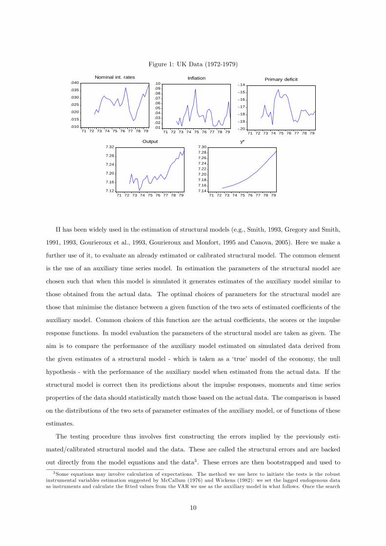
Figure 1: UK Data (1972-1979)

7.12

7.16

7.20

7.24

7.28

7.32

71 72 73 74 75 76 77 78 79

Output

7.147.167.187.207.227.247.267.287.30

71 72 73 74 75 76 77 78 79

y*

.01

.02

.03

.04

.05

.06

.07

.08

.09

.10

71 72 73 74 75 76 77 78 79

Inflation

.010

.015

.020

.025

.030

.035

.040

71 72 73 74 75 76 77 78 79

Nominal int. rates

­.20

­.19

­.18

­.17

­.16

­.15

­.14

71 72 73 74 75 76 77 78 79

Primary deficit

II has been widely used in the estimation of structural models (e.g., Smith, 1993, Gregory and Smith,

1991, 1993, Gourieroux et al., 1993, Gourieroux and Monfort, 1995 and Canova, 2005). Here we make a

further use of it, to evaluate an already estimated or calibrated structural model. The common element

is the use of an auxiliary time series model. In estimation the parameters of the structural model are

chosen such that when this model is simulated it generates estimates of the auxiliary model similar to

those obtained from the actual data. The optimal choices of parameters for the structural model are

those that minimise the distance between a given function of the two sets of estimated coe¢ cients of the

auxiliary model. Common choices of this function are the actual coe¢ cients, the scores or the impulse

response functions. In model evaluation the parameters of the structural model are taken as given. The

aim is to compare the performance of the auxiliary model estimated on simulated data derived from

the given estimates of a structural model - which is taken as a �true�model of the economy, the null

hypothesis - with the performance of the auxiliary model when estimated from the actual data. If the

structural model is correct then its predictions about the impulse responses, moments and time series

properties of the data should statistically match those based on the actual data. The comparison is based

on the distributions of the two sets of parameter estimates of the auxiliary model, or of functions of these

estimates.

The testing procedure thus involves �rst constructing the errors implied by the previously esti-

mated/calibrated structural model and the data. These are called the structural errors and are backed

out directly from the model equations and the data3 . These errors are then bootstrapped and used to

3Some equations may involve calculation of expectations. The method we use here to initiate the tests is the robustinstrumental variables estimation suggested by McCallum (1976) and Wickens (1982): we set the lagged endogenous dataas instruments and calculate the �tted values from the VAR we use as the auxiliary model in what follows. Once the search

10

generate for each bootstrap new data based on the structural model. An auxiliary time series model

is then �tted to each set of data and the sampling distribution of the coe¢ cients of the auxiliary time

series model is obtained from these estimates of the auxiliary model. A Wald statistic is computed to

determine whether functions of the parameters of the time series model estimated on the actual data lie

in some con�dence interval implied by this sampling distribution.

The auxiliary model should be a process that would describe the evolution of the data under any

relevant model. It is known that for non-stationary data the reduced form of a macro model is a VARMA

where non-stationary forcing variables enter as conditioning variables to achieve cointegration (i.e. en-

suring that the stochastic trends in the endogenous vector are picked up so that the errors in the VAR

are stationary). This in turn can be approximated as a VECM4 . So following Meenagh et al. (2012)

procedure (e¤ectively indirect estimation) has converged on the best model parameters, we then move to generating theexpectations exactly implied by the parameters and the data, and use these to calculate the errors, which are then the exacterrors implied by the model and data. The reason we do not use this �exact�method at the start is that initially when themodel is far from the data, the expectations generated are also far from the true ones, so that the errors are exaggeratedand the procedure may not converge.

4Following Meenagh et al. (2012), we can say that after log-linearisation a DSGE model can usually be written in theform

A(L)yt = BEtyt+1 + C(L)xt +D(L)et (A1)

where yt are p endogenous variables and xt are q exogenous variables which we assume are driven by

�xt = a(L)�xt�1 + d+ c(L)�t: (A2)

The exogenous variables may contain both observable and unobservable variables such as a technology shock. The distur-bances et and �t are both iid variables with zero means. It follows that both yt and xt are non-stationary. L denotes thelag operator zt�s = Lszt and A(L), B(L) etc. are polynomial functions with roots outside the unit circle.The general solution of yt is

yt = G(L)yt�1 +H(L)xt + f +M(L)et +N(L)�t: (A3)

where the polynomial functions have roots outside the unit circle. As yt and xt are non-stationary, the solution has the p

cointegration relations

yt = [I �G(1)]�1[H(1)xt + f ]= �xt + g: (A4)

The long-run solution to the model is

yt = �xt + g

xt = [1� a(1)]�1[dt+ c(1)�t]�t = �t�1i=0�t�s

Hence the long-run solution to xt, namely, xt = xDt + xSt has a deterministic trend xDt = [1 � a(1)]�1dt and a stochastic

trend xSt = [1� a(1)]�1c(1)�t.The solution for yt can therefore be re-written as the VECM

�yt = �[I �G(1)](yt�1 ��xt�1) + P (L)�yt�1 +Q(L)�xt + f +M(L)et +N(L)�t

= �[I �G(1)](yt�1 ��xt�1) + P (L)�yt�1 +Q(L)�xt + f + !t (A5)

!t = M(L)et +N(L)�t

Hence, in general, the disturbance !t is a mixed moving average process. This suggests that the VECM can be approximatedby the VARX

�yt = K(yt�1 ��xt�1) +R(L)�yt�1 + S(L)�xt + g + �t (A6)

where �t is an iid zero-mean process.As

xt = xt�1 + [1� a(1)]�1[d+ �t]the VECM can also be written as

�yt = K[(yt�1 � yt�1)��(xt�1 � xt�1)] +R(L)�yt�1 + S(L)�xt + h+ �t: (A7)

Either equations (A6) or (A7) can act as the auxiliary model. Here we focus on (A7); this distinguishes between the e¤ectof the trend element in x and the temporary deviation from its trend. In our models these two elements have di¤erent

11

we use as the auxiliary model a VECM which we reexpress as a VARX(1) for the four macro variables

(interest rate, output, in�ation and the primary budget de�cit, with a time trend and with y�t entered

as the exogenous non-stationary �productivity trend�(these two elements having the e¤ect of achieving

cointegration). Thus our auxiliary model in practice is given by: yt = [I�K]yt�1+ xt�1+gt+vt where

xt�1 is the stochastic trend in productivity, gt are the deterministic trends, and vt are the VECM inno-

vations. We treat as the descriptors of the data all the VARX coe¢ cients and the VARX error variances.

From these a Wald statistic may be computed that acts as a test at a given con�dence level of whether

the observed dynamics, volatility and cointegrating relations of the chosen variables are explained by the

DSGE-model-simulated joint distribution of these. This Wald statistic is given by:

(�� �)0X�1

(��)(�� �) (1)

where � is the vector of VARX estimates of the chosen descriptors yielded in each simulation, with � andP(��) representing the corresponding sample means and variance-covariance matrix of these calculated

across simulations, respectively.

The joint distribution of the � is obtained by bootstrapping the innovations implied by the data and

the theoretical model; it is therefore an estimate of the small sample distribution5 . Such a distribution

is generally more accurate for small samples than the asymptotic distribution; it is also shown to be

consistent by Le et al. (2011) given that the Wald statistic is �asymptotically pivotal�; they also showed

it had quite good accuracy in small sample Monte Carlo experiments6 .

This testing procedure is applied to a set of (structural) parameters put forward as the true ones

(H0, the null hypothesis); they can be derived from calibration, estimation, or both. However derived,

the test then asks: could these coe¢ cients within this model structure be the true (numerical) model

generating the data? Of course only one true model with one set of coe¢ cients is possible. Nevertheless

we may have chosen coe¢ cients that are not exactly right numerically, so that the same model with other

coe¢ cient values could be correct. Only when we have examined the model with all coe¢ cient values

that are feasible within the model theory will we have properly tested it. For this reason we extend our

procedure by a further search algorithm, in which we seek other coe¢ cient sets that minimise the Wald

test statistic - in doing this we are carrying out indirect estimation. The indirect estimates of the model

are consistent and asymptotically normal, in common with FIML - see Smith (1993), Gregory and Smith

e¤ects and so should be distinguished in the data to allow the greatest test discrimination.It is possible to estimate (A7) in one stage by OLS. Meenagh et al. (2012) do Monte Carlo experiments to check this

procedure and �nd it to be extremely accurate.5The bootstraps in our tests are all drawn as time vectors so contemporaneous correlations between the innovations are

preserved.6Speci�cally, they found on stationary data that the bias due to bootstrapping was just over 2% at the 95% con�dence

level and 0.6% at the 99% level. Meenagh et al (2012) found even greater accuracy in Monte Carlo experiments onnonstationary data.

12

(1991, 1993), Gourieroux et al., (1993), Gourieroux and Monfort (1995) and Canova (2005).

Thus we calculate the minimum-value full Wald statistic for each model using a powerful algorithm

based on Simulated Annealing (SA) in which search takes place over a wide range around the initial

values, with optimising search accompanied by random jumps around the space7 . The merit of this

extended procedure is that we are comparing the best possible versions of each model type when �nally

doing our comparison of model compatibility with the data.

4.1.1 Model results under II

We now turn to the empirical performance of the competing models outlined above under II. We sum-

marise the model estimates (by Simulated Annealing) in table 2 (The Wald test results based on these

are shown in table 6 in what follows).

Table 2: Indirect estimates of the FTPL and the Orthodox models

Model parameter Starting value FTPL Orthodox Taylor� 2.4 4.07 1.96� 0.99 �xed �xed� 2.27 0.02 0.46� 0.26 0.35 -� 0.5 - 0.76�� 2 - 1.31�xgap 0.125 - 0.06� 0.003 - 0.007cy� 0.0002 �xed �xed 0.99 �xed �xed

Shock persistence (rho�s)errpp - 0.43 0.42errIS - 0.64 0.84erry� - 0.93 0.93errg�t - -0.1 -0.1err� - 0.24 -

errRS

- - 0.33

The estimates for the two models�shared parameters (� and �) are strikingly di¤erent. In the FTPL

� is high and � is low, implying a steep Phillips curve and a �at IS curve. Since in�ation is determined

exogenously by the exogenous de�cit ratio and its own error process, the steep Phillips curve (which

determines the output gap) implies that the output gap responds weakly to in�ation while the �at IS

curve (which sets interest rates) implies that the real interest rate responds weakly to the output gap.

7We use a Simulated Annealing algorithm due to Ingber (1996). This mimics the behaviour of the steel cooling processin which steel is cooled, with a degree of reheating at randomly chosen moments in the cooling process� this ensuring thatthe defects are minimised globally. Similarly the algorithm searches in the chosen range and as points that improve theobjective are found it also accepts points that do not improve the objective. This helps to stop the algorithm being caught inlocal minima. We �nd this algorithm improves substantially here on a standard optimisation algorithm. Our method usedour standard testing method: we take a set of model parameters (excluding error processes), extract the resulting residualsfrom the data using the LIML method, �nd their implied autoregressive coe¢ cients (AR(1) here) and then bootstrap theimplied innovations with this full set of parameters to �nd the implied Wald value. This is then minimised by the SAalgorithm.

13

The impulse response functions for the FTPL model (�gures 2-5) con�rm this8 .

Figure 2: IRFs - Output (FTPL)

­0.02

­0.015

­0.01

­0.005

0

0.005

0 1 2 3 4 5 6 7 8 9 10

err(PP)

err(pi)

err(g­t)

Figure 3: IRFs - In�ation (FTPL)

0

0.004

0.008

0.012

0.016

0.02

0 1 2 3 4 5 6 7 8 9 10

err(PP)

err(pi)

err(g­t)

Figure 4: IRFs - Nom. int. rates (FTPL)

0

0.001

0.002

0.003

0.004

0.005

0.006

0 1 2 3 4 5 6 7 8 9 10

err(IS)

err(PP)

err(pi)

err(g­t)

E¤ectively this suppresses most of the simultaneity in the model as can be seen from the variance

decomposition in table 3. We �nd this by bootstrapping the innovations of the model repeatedly for the

same sample episode - plainly the variances of non-stationary variables, while unde�ned asymptotically,

are de�ned for this (short) sample period. One sees that in�ation is disturbed by both the �scal de�cit

and its own shock; output by both the productivity trend and the supply (errPP ) shock, with a minimal

8 In this model the e¤ect of IS curve shock on output and in�ation is nil.

14

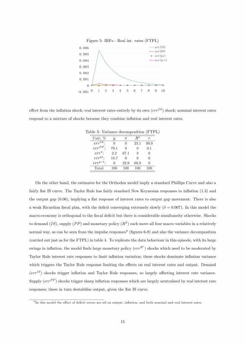
Figure 5: IRFs - Real int. rates (FTPL)

­0.001

0

0.001

0.002

0.003

0.004

0.005

0.006

0 1 2 3 4 5 6 7 8 9 10

err(IS)

err(PP)

err(pi)

err(g­t)

e¤ect from the in�ation shock; real interest rates entirely by its own (errIS) shock; nominal interest rates

respond to a mixture of shocks because they combine in�ation and real interest rates.

Table 3: Variance decomposition (FTPL)

Unit: % y � Rs rerrIS : 0 0 23.1 99.9errPP : 79.1 0 0 0.1err� : 2.2 67.1 8 0erry�: 18.7 0 0 0errg�t: 0 32.9 68.9 0Total: 100 100 100 100

On the other hand, the estimates for the Orthodox model imply a standard Phillips Curve and also a

fairly �at IS curve. The Taylor Rule has fairly standard New Keynesian responses to in�ation (1.3) and

the output gap (0.06), implying a �at response of interest rates to output gap movement. There is also

a weak Ricardian �scal plan, with the de�cit converging extremely slowly (� = 0:007). In this model the

macro-economy is orthogonal to the �scal de�cit but there is considerable simultaneity otherwise. Shocks

to demand (IS), supply (PP ) and monetary policy (RS) each move all four macro variables in a relatively

normal way, as can be seen from the impulse responses9 (�gures 6-9) and also the variance decomposition

(carried out just as for the FTPL) in table 4. To replicate the data behaviour in this episode, with its large

swings in in�ation, the model �nds large monetary policy (errRs

) shocks which need to be moderated by

Taylor Rule interest rate responses to limit in�ation variation; these shocks dominate in�ation variance

which triggers the Taylor Rule response limiting the e¤ects on real interest rates and output. Demand

(errIS) shocks trigger in�ation and Taylor Rule responses, so largely a¤ecting interest rate variance.

Supply (errPP ) shocks trigger sharp in�ation responses which are largely neutralised by real interest rate

responses; these in turn destabilise output, given the �at IS curve.

9 In this model the e¤ect of de�cit errors are nil on output, in�ation, and both nominal and real interest rates.

15

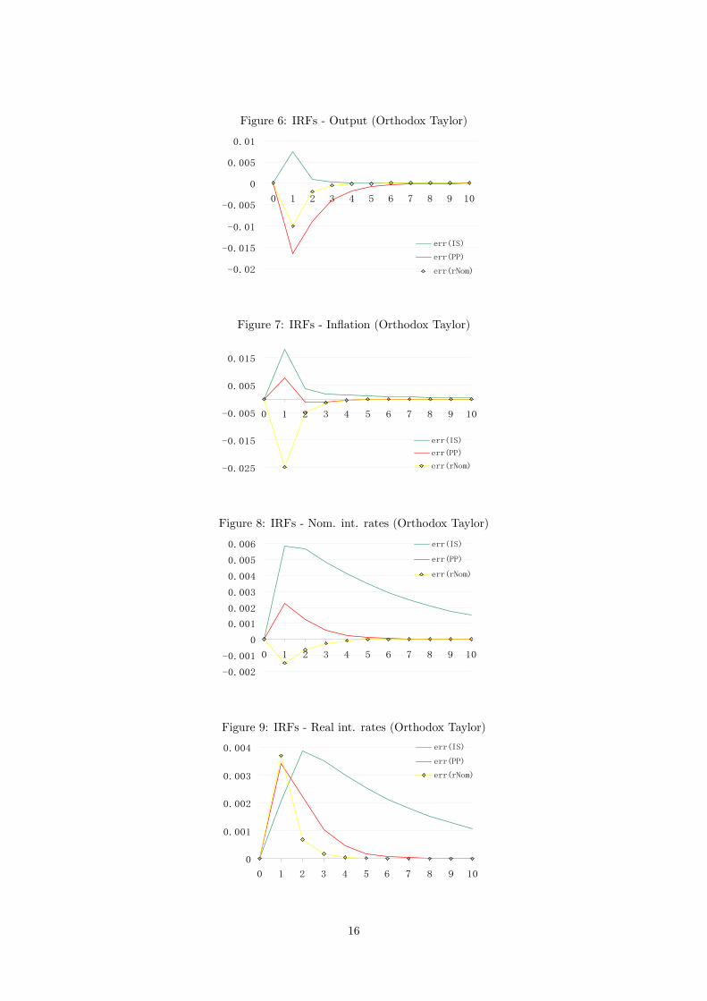
Figure 6: IRFs - Output (Orthodox Taylor)

­0.02

­0.015

­0.01

­0.005

0

0.005

0.01

0 1 2 3 4 5 6 7 8 9 10

err(IS)

err(PP)

err(rNom)

Figure 7: IRFs - In�ation (Orthodox Taylor)

­0.025

­0.015

­0.005

0.005

0.015

0 1 2 3 4 5 6 7 8 9 10

err(IS)

err(PP)

err(rNom)

Figure 8: IRFs - Nom. int. rates (Orthodox Taylor)

­0.002

­0.001

0

0.001

0.002

0.003

0.004

0.005

0.006

0 1 2 3 4 5 6 7 8 9 10

err(IS)

err(PP)

err(rNom)

Figure 9: IRFs - Real int. rates (Orthodox Taylor)

0

0.001

0.002

0.003

0.004

0 1 2 3 4 5 6 7 8 9 10

err(IS)

err(PP)

err(rNom)

16

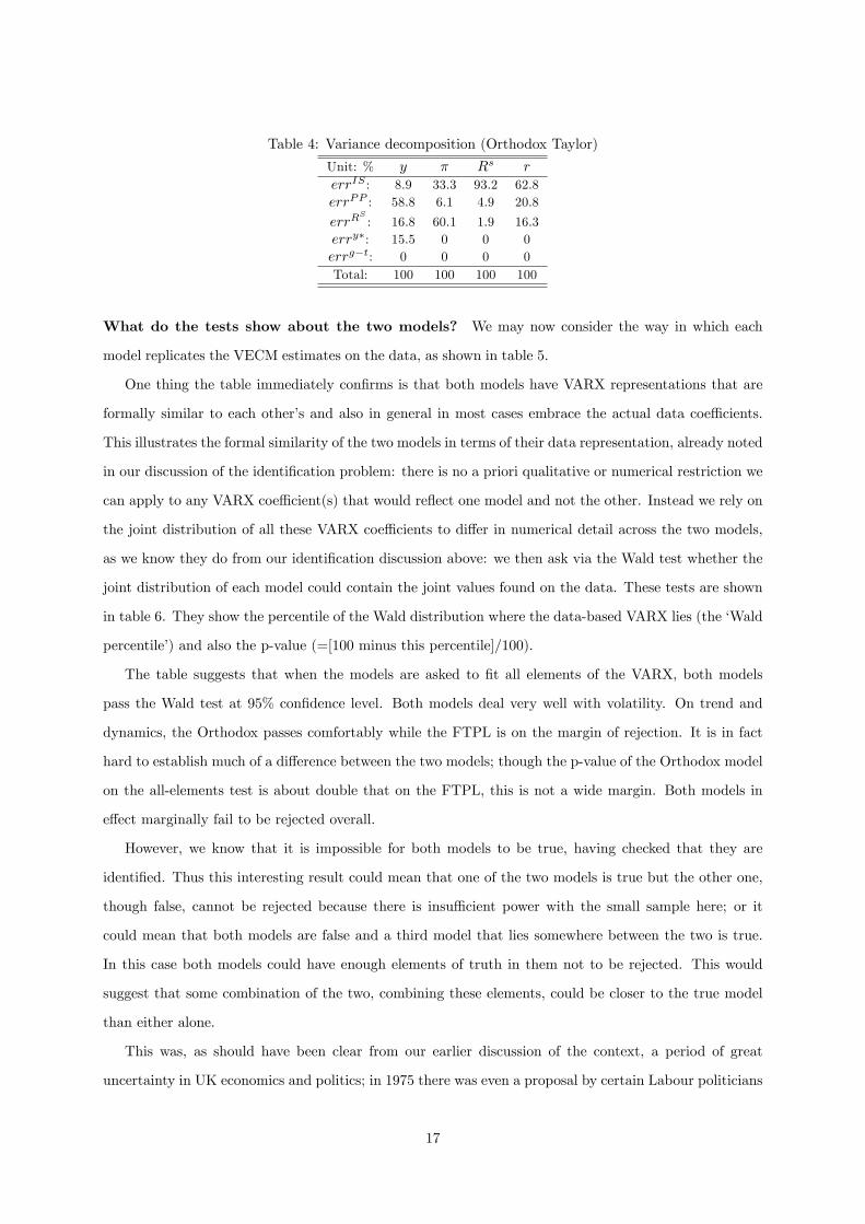
Table 4: Variance decomposition (Orthodox Taylor)

Unit: % y � Rs rerrIS : 8.9 33.3 93.2 62.8errPP : 58.8 6.1 4.9 20.8

errRS

: 16.8 60.1 1.9 16.3erry�: 15.5 0 0 0errg�t: 0 0 0 0Total: 100 100 100 100

What do the tests show about the two models? We may now consider the way in which each

model replicates the VECM estimates on the data, as shown in table 5.

One thing the table immediately con�rms is that both models have VARX representations that are

formally similar to each other�s and also in general in most cases embrace the actual data coe¢ cients.

This illustrates the formal similarity of the two models in terms of their data representation, already noted

in our discussion of the identi�cation problem: there is no a priori qualitative or numerical restriction we

can apply to any VARX coe¢ cient(s) that would re�ect one model and not the other. Instead we rely on

the joint distribution of all these VARX coe¢ cients to di¤er in numerical detail across the two models,

as we know they do from our identi�cation discussion above: we then ask via the Wald test whether the

joint distribution of each model could contain the joint values found on the data. These tests are shown

in table 6. They show the percentile of the Wald distribution where the data-based VARX lies (the �Wald

percentile�) and also the p-value (=[100 minus this percentile]/100).

The table suggests that when the models are asked to �t all elements of the VARX, both models

pass the Wald test at 95% con�dence level. Both models deal very well with volatility. On trend and

dynamics, the Orthodox passes comfortably while the FTPL is on the margin of rejection. It is in fact

hard to establish much of a di¤erence between the two models; though the p-value of the Orthodox model

on the all-elements test is about double that on the FTPL, this is not a wide margin. Both models in

e¤ect marginally fail to be rejected overall.

However, we know that it is impossible for both models to be true, having checked that they are

identi�ed. Thus this interesting result could mean that one of the two models is true but the other one,

though false, cannot be rejected because there is insu¢ cient power with the small sample here; or it

could mean that both models are false and a third model that lies somewhere between the two is true.

In this case both models could have enough elements of truth in them not to be rejected. This would

suggest that some combination of the two, combining these elements, could be closer to the true model

than either alone.

This was, as should have been clear from our earlier discussion of the context, a period of great

uncertainty in UK economics and politics; in 1975 there was even a proposal by certain Labour politicians

17

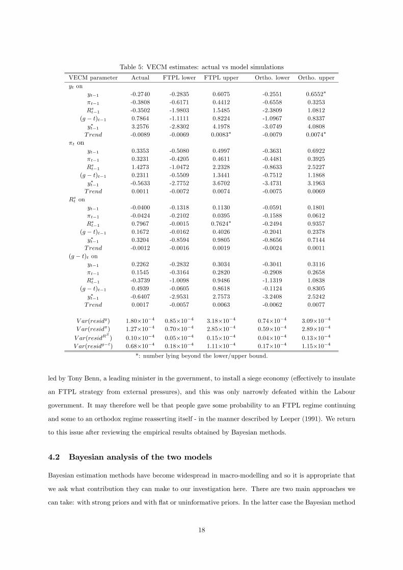
Table 5: VECM estimates: actual vs model simulations

VECM parameter Actual FTPL lower FTPL upper Ortho. lower Ortho. upperyt on

yt�1 -0.2740 -0.2835 0.6075 -0.2551 0.6552�

�t�1 -0.3808 -0.6171 0.4412 -0.6558 0.3253Rst�1 -0.3502 -1.9803 1.5485 -2.3809 1.0812

(g � t)t�1 0.7864 -1.1111 0.8224 -1.0967 0.8337y�t�1 3.2576 -2.8302 4.1978 -3.0749 4.0808Trend -0.0089 -0.0069 0.0083� -0.0079 0.0074�

�t onyt�1 0.3353 -0.5080 0.4997 -0.3631 0.6922�t�1 0.3231 -0.4205 0.4611 -0.4481 0.3925Rst�1 1.4273 -1.0472 2.2328 -0.8633 2.5227

(g � t)t�1 0.2311 -0.5509 1.3441 -0.7512 1.1868y�t�1 -0.5633 -2.7752 3.6702 -3.4731 3.1963Trend 0.0011 -0.0072 0.0074 -0.0075 0.0069

Rst onyt�1 -0.0400 -0.1318 0.1130 -0.0591 0.1801�t�1 -0.0424 -0.2102 0.0395 -0.1588 0.0612Rst�1 0.7967 -0.0015 0.7624� -0.2494 0.9357

(g � t)t�1 0.1672 -0.0162 0.4026 -0.2041 0.2378y�t�1 0.3204 -0.8594 0.9805 -0.8656 0.7144Trend -0.0012 -0.0016 0.0019 -0.0024 0.0011

(g � t)t onyt�1 0.2262 -0.2832 0.3034 -0.3041 0.3116�t�1 0.1545 -0.3164 0.2820 -0.2908 0.2658Rst�1 -0.3739 -1.0098 0.9486 -1.1319 1.0838

(g � t)t�1 0.4939 -0.0605 0.8618 -0.1124 0.8305y�t�1 -0.6407 -2.9531 2.7573 -3.2408 2.5242Trend 0.0017 -0.0057 0.0063 -0.0062 0.0077

V ar(residy) 1.80�10�4 0.85�10�4 3.18�10�4 0.74�10�4 3.09�10�4V ar(resid�) 1.27�10�4 0.70�10�4 2.85�10�4 0.59�10�4 2.89�10�4

V ar(residRS

) 0.10�10�4 0.05�10�4 0.15�10�4 0.04�10�4 0.13�10�4V ar(residg�t) 0.68�10�4 0.18�10�4 1.11�10�4 0.17�10�4 1.15�10�4

*: number lying beyond the lower/upper bound.

led by Tony Benn, a leading minister in the government, to install a siege economy (e¤ectively to insulate

an FTPL strategy from external pressures), and this was only narrowly defeated within the Labour

government. It may therefore well be that people gave some probability to an FTPL regime continuing

and some to an orthodox regime reasserting itself - in the manner described by Leeper (1991). We return

to this issue after reviewing the empirical results obtained by Bayesian methods.

4.2 Bayesian analysis of the two models

Bayesian estimation methods have become widespread in macro-modelling and so it is appropriate that

we ask what contribution they can make to our investigation here. There are two main approaches we

can take: with strong priors and with �at or uninformative priors. In the latter case the Bayesian method

18

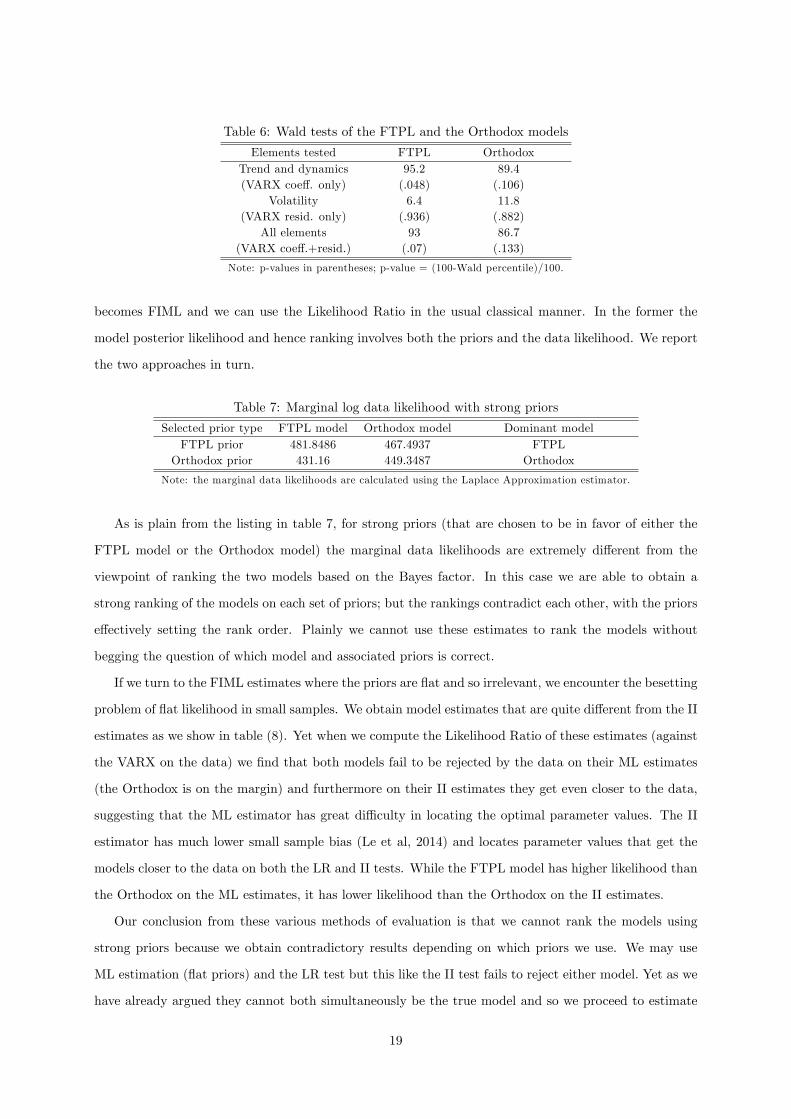
Table 6: Wald tests of the FTPL and the Orthodox models

Elements tested FTPL OrthodoxTrend and dynamics(VARX coe¤. only)

95.2(.048)

89.4(.106)

Volatility(VARX resid. only)

6.4(.936)

11.8(.882)

All elements(VARX coe¤.+resid.)

93(.07)

86.7(.133)

Note: p-values in parentheses; p-value = (100-Wald percentile)/100.

becomes FIML and we can use the Likelihood Ratio in the usual classical manner. In the former the

model posterior likelihood and hence ranking involves both the priors and the data likelihood. We report

the two approaches in turn.

Table 7: Marginal log data likelihood with strong priors

Selected prior type FTPL model Orthodox model Dominant modelFTPL prior 481.8486 467.4937 FTPL

Orthodox prior 431.16 449.3487 Orthodox

Note: the marginal data likelihoods are calculated using the Laplace Approximation estimator.

As is plain from the listing in table 7, for strong priors (that are chosen to be in favor of either the

FTPL model or the Orthodox model) the marginal data likelihoods are extremely di¤erent from the

viewpoint of ranking the two models based on the Bayes factor. In this case we are able to obtain a

strong ranking of the models on each set of priors; but the rankings contradict each other, with the priors

e¤ectively setting the rank order. Plainly we cannot use these estimates to rank the models without

begging the question of which model and associated priors is correct.

If we turn to the FIML estimates where the priors are �at and so irrelevant, we encounter the besetting

problem of �at likelihood in small samples. We obtain model estimates that are quite di¤erent from the II

estimates as we show in table (8). Yet when we compute the Likelihood Ratio of these estimates (against

the VARX on the data) we �nd that both models fail to be rejected by the data on their ML estimates

(the Orthodox is on the margin) and furthermore on their II estimates they get even closer to the data,

suggesting that the ML estimator has great di¢ culty in locating the optimal parameter values. The II

estimator has much lower small sample bias (Le et al, 2014) and locates parameter values that get the

models closer to the data on both the LR and II tests. While the FTPL model has higher likelihood than

the Orthodox on the ML estimates, it has lower likelihood than the Orthodox on the II estimates.

Our conclusion from these various methods of evaluation is that we cannot rank the models using

strong priors because we obtain contradictory results depending on which priors we use. We may use

ML estimation (�at priors) and the LR test but this like the II test fails to reject either model. Yet as we

have already argued they cannot both simultaneously be the true model and so we proceed to estimate

19

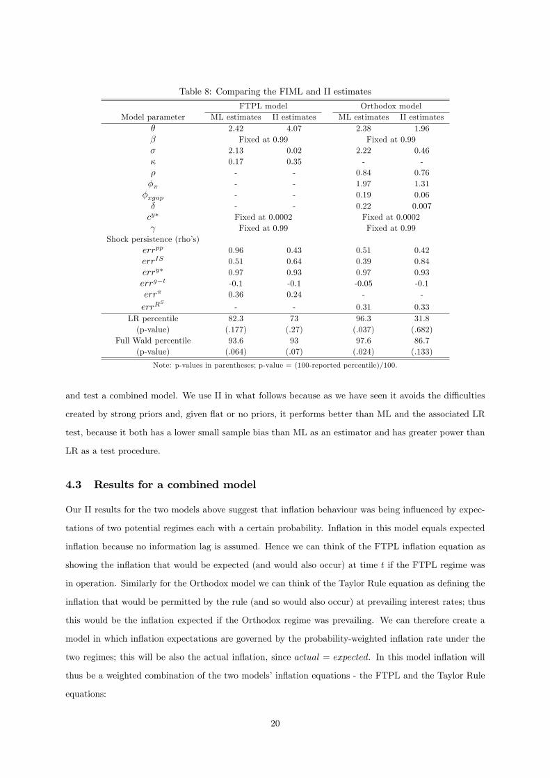
Table 8: Comparing the FIML and II estimates

FTPL model Orthodox modelModel parameter ML estimates II estimates ML estimates II estimates

� 2.42 4.07 2.38 1.96� Fixed at 0.99 Fixed at 0.99� 2.13 0.02 2.22 0.46� 0.17 0.35 - -� - - 0.84 0.76�� - - 1.97 1.31�xgap - - 0.19 0.06� - - 0.22 0.007cy� Fixed at 0.0002 Fixed at 0.0002 Fixed at 0.99 Fixed at 0.99

Shock persistence (rho�s)errpp 0.96 0.43 0.51 0.42errIS 0.51 0.64 0.39 0.84erry� 0.97 0.93 0.97 0.93errg�t -0.1 -0.1 -0.05 -0.1err� 0.36 0.24 - -

errRS

- - 0.31 0.33LR percentile(p-value)

82.3(.177)

73(.27)

96.3(.037)

31.8(.682)

Full Wald percentile(p-value)

93.6(.064)

93(.07)

97.6(.024)

86.7(.133)

Note: p-values in parentheses; p-value = (100-reported percentile)/100.

and test a combined model. We use II in what follows because as we have seen it avoids the di¢ culties

created by strong priors and, given �at or no priors, it performs better than ML and the associated LR

test, because it both has a lower small sample bias than ML as an estimator and has greater power than

LR as a test procedure.

4.3 Results for a combined model

Our II results for the two models above suggest that in�ation behaviour was being in�uenced by expec-

tations of two potential regimes each with a certain probability. In�ation in this model equals expected

in�ation because no information lag is assumed. Hence we can think of the FTPL in�ation equation as

showing the in�ation that would be expected (and would also occur) at time t if the FTPL regime was

in operation. Similarly for the Orthodox model we can think of the Taylor Rule equation as de�ning the

in�ation that would be permitted by the rule (and so would also occur) at prevailing interest rates; thus

this would be the in�ation expected if the Orthodox regime was prevailing. We can therefore create a

model in which in�ation expectations are governed by the probability-weighted in�ation rate under the

two regimes; this will be also the actual in�ation, since actual = expected. In this model in�ation will

thus be a weighted combination of the two models�in�ation equations - the FTPL and the Taylor Rule

equations:

20

(16)

�t = WFTPL�(gt � tt)

+[1�WFTPL]1

��[

1

(1� �) (Rt � �Rt�1)� �xgap(yt � y�t )� �] + err

Weighted �t

Given that in�ation is determined by the probability-weighted average of each regime�s own in�ation

outcome, we now have a composite in�ation error - which in principle consists of the weighted combi-

nation of the two regime error processes plus any temporary deviations of in�ation from this weighted

combination (e.g. due to variation in the weight). Since we cannot observe what the in�ation rate actually

was in each regime, only the average outcome, we can only observe a composite error.

All the other equations are the same, with the exception of the �scal de�cit equation which has an AR

coe¢ cient (� = 0:007, as reported in table 2) that is so close to zero that it cannot resolve the uncertainty

about which regime is operating; we allow it to be determined by the model estimation.

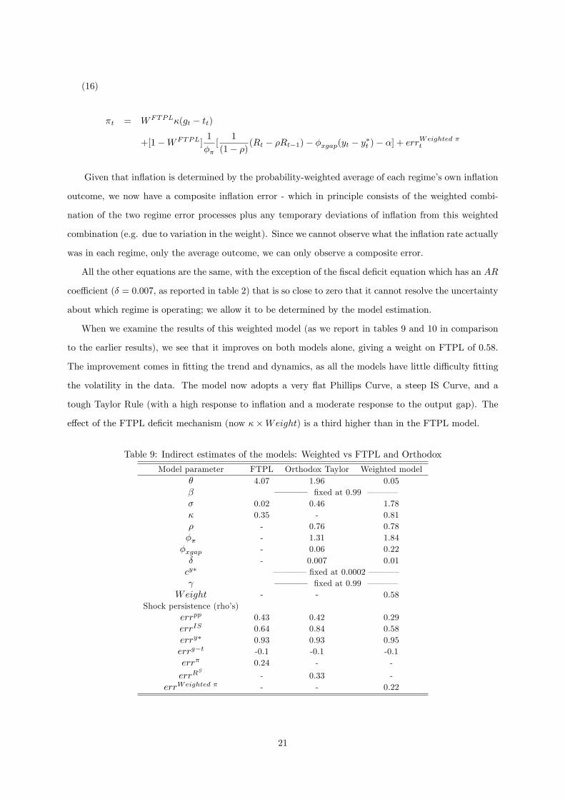
When we examine the results of this weighted model (as we report in tables 9 and 10 in comparison

to the earlier results), we see that it improves on both models alone, giving a weight on FTPL of 0.58.

The improvement comes in �tting the trend and dynamics, as all the models have little di¢ culty �tting

the volatility in the data. The model now adopts a very �at Phillips Curve, a steep IS Curve, and a

tough Taylor Rule (with a high response to in�ation and a moderate response to the output gap). The

e¤ect of the FTPL de�cit mechanism (now ��Weight) is a third higher than in the FTPL model.

Table 9: Indirect estimates of the models: Weighted vs FTPL and Orthodox

Model parameter FTPL Orthodox Taylor Weighted model� 4.07 1.96 0.05� � � � � �xed at 0.99 � � � �� 0.02 0.46 1.78� 0.35 - 0.81� - 0.76 0.78�� - 1.31 1.84�xgap - 0.06 0.22� - 0.007 0.01cy� � � � ��xed at 0.0002 � � � � � � � � �xed at 0.99 � � � �

Weight - - 0.58Shock persistence (rho�s)

errpp 0.43 0.42 0.29errIS 0.64 0.84 0.58erry� 0.93 0.93 0.95errg�t -0.1 -0.1 -0.1err� 0.24 - -

errRS

- 0.33 -errWeighted � - - 0.22

21

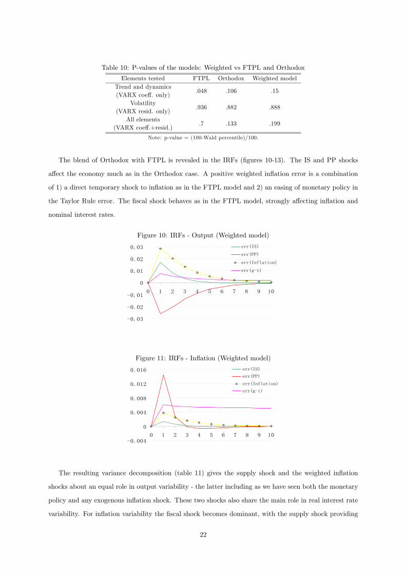
Table 10: P-values of the models: Weighted vs FTPL and Orthodox

Elements tested FTPL Orthodox Weighted modelTrend and dynamics(VARX coe¤. only)

.048 .106 .15

Volatility(VARX resid. only)

.936 .882 .888

All elements(VARX coe¤.+resid.)

.7 .133 .199

Note: p-value = (100-Wald percentile)/100.

The blend of Orthodox with FTPL is revealed in the IRFs (�gures 10-13). The IS and PP shocks

a¤ect the economy much as in the Orthodox case. A positive weighted in�ation error is a combination

of 1) a direct temporary shock to in�ation as in the FTPL model and 2) an easing of monetary policy in

the Taylor Rule error. The �scal shock behaves as in the FTPL model, strongly a¤ecting in�ation and

nominal interest rates.

Figure 10: IRFs - Output (Weighted model)

­0.03

­0.02

­0.01

0

0.01

0.02

0.03

0 1 2 3 4 5 6 7 8 9 10

err(IS)

err(PP)

err(Inflation)

err(g­t)

Figure 11: IRFs - In�ation (Weighted model)

­0.004

0

0.004

0.008

0.012

0.016

0 1 2 3 4 5 6 7 8 9 10

err(IS)

err(PP)

err(Inflation)

err(g­t)

The resulting variance decomposition (table 11) gives the supply shock and the weighted in�ation

shocks about an equal role in output variability - the latter including as we have seen both the monetary

policy and any exogenous in�ation shock. These two shocks also share the main role in real interest rate

variability. For in�ation variability the �scal shock becomes dominant, with the supply shock providing

22

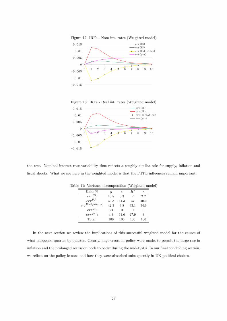
Figure 12: IRFs - Nom int. rates (Weighted model)

­0.015

­0.01

­0.005

0

0.005

0.01

0.015

0 1 2 3 4 5 6 7 8 9 10

err(IS)

err(PP)

err(Inflation)

err(g­t)

Figure 13: IRFs - Real int. rates (Weighted model)

­0.015

­0.01

­0.005

0

0.005

0.01

0.015

0 1 2 3 4 5 6 7 8 9 10

err(IS)

err(PP)

err(Inflation)

err(g­t)

the rest. Nominal interest rate variability thus re�ects a roughly similar role for supply, in�ation and

�scal shocks. What we see here in the weighted model is that the FTPL in�uences remain important.

Table 11: Variance decomposition (Weighted model)

Unit: % y � Rs rerrIS : 10.8 0.3 2 2.2errPP : 39.3 34.3 37 40.2

errWeighted � : 42.3 3.8 33.1 54.6erry�: 3.4 0 0 0errg�t: 4.3 61.6 27.9 3Total: 100 100 100 100

In the next section we review the implications of this successful weighted model for the causes of

what happened quarter by quarter. Clearly, huge errors in policy were made, to permit the large rise in

in�ation and the prolonged recession both to occur during the mid-1970s. In our �nal concluding section,

we re�ect on the policy lessons and how they were absorbed subsequently in UK political choices.

23

5 A time-line of the UK 1970s episode according to the weighted

model

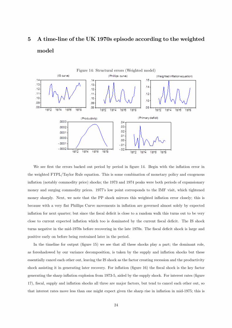
Figure 14: Structural errors (Weighted model)

We see �rst the errors backed out period by period in �gure 14. Begin with the in�ation error in

the weighted FTPL/Taylor Rule equation. This is some combination of monetary policy and exogenous

in�ation (notably commodity price) shocks; the 1973 and 1974 peaks were both periods of expansionary

money and surging commodity prices. 1977�s low point corresponds to the IMF visit, which tightened

money sharply. Next, we note that the PP shock mirrors this weighted in�ation error closely; this is

because with a very �at Phillips Curve movements in in�ation are governed almost solely by expected

in�ation for next quarter; but since the �scal de�cit is close to a random walk this turns out to be very

close to current expected in�ation which too is dominated by the current �scal de�cit. The IS shock

turns negative in the mid-1970s before recovering in the late 1970s. The �scal de�cit shock is large and

positive early on before being restrained later in the period.

In the timeline for output (�gure 15) we see that all these shocks play a part; the dominant role,

as foreshadowed by our variance decomposition, is taken by the supply and in�ation shocks but these

essentially cancel each other out, leaving the IS shock as the factor creating recession and the productivity

shock assisting it in generating later recovery. For in�ation (�gure 16) the �scal shock is the key factor

generating the sharp in�ation explosion from 1973-5, aided by the supply shock. For interest rates (�gure

17), �scal, supply and in�ation shocks all three are major factors, but tend to cancel each other out, so

that interest rates move less than one might expect given the sharp rise in in�ation in mid-1975; this is

24

Figure 15: Timeline for output (Weighted model)

­0.10­0.08­0.06­0.04­0.020.00

0.020.040.060.080.100.12

1973Q3 1974Q3 1975Q3 1976Q3 1977Q3 1978Q3 1979Q3

err(IS) err(PP) err(Weighted pi)err(y*) err(g­t) Total

Figure 16: Timeline for in�ation (Weighted model)

­0.06

­0.04

­0.02

0.00

0.02

0.04

0.06

0.08

1973Q3 1974Q3 1975Q3 1976Q3 1977Q3 1978Q3 1979Q3

err(IS) err(PP) err(Weighted pi)

err(g­t) Total

25

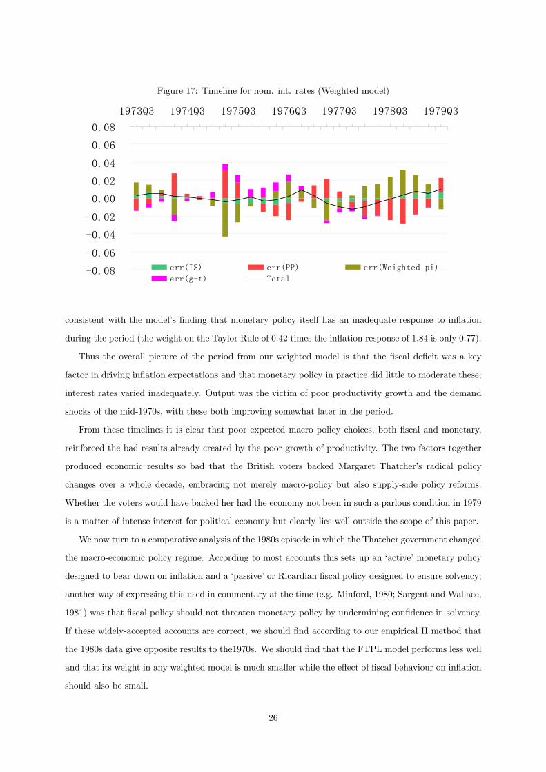
Figure 17: Timeline for nom. int. rates (Weighted model)

­0.08

­0.06

­0.04

­0.02

0.00

0.02

0.04

0.06

0.08

1973Q3 1974Q3 1975Q3 1976Q3 1977Q3 1978Q3 1979Q3

err(IS) err(PP) err(Weighted pi)

err(g­t) Total

consistent with the model�s �nding that monetary policy itself has an inadequate response to in�ation

during the period (the weight on the Taylor Rule of 0.42 times the in�ation response of 1.84 is only 0.77).

Thus the overall picture of the period from our weighted model is that the �scal de�cit was a key

factor in driving in�ation expectations and that monetary policy in practice did little to moderate these;

interest rates varied inadequately. Output was the victim of poor productivity growth and the demand

shocks of the mid-1970s, with these both improving somewhat later in the period.

From these timelines it is clear that poor expected macro policy choices, both �scal and monetary,

reinforced the bad results already created by the poor growth of productivity. The two factors together

produced economic results so bad that the British voters backed Margaret Thatcher�s radical policy

changes over a whole decade, embracing not merely macro-policy but also supply-side policy reforms.

Whether the voters would have backed her had the economy not been in such a parlous condition in 1979

is a matter of intense interest for political economy but clearly lies well outside the scope of this paper.

We now turn to a comparative analysis of the 1980s episode in which the Thatcher government changed

the macro-economic policy regime. According to most accounts this sets up an �active�monetary policy

designed to bear down on in�ation and a �passive�or Ricardian �scal policy designed to ensure solvency;

another way of expressing this used in commentary at the time (e.g. Minford, 1980; Sargent and Wallace,

1981) was that �scal policy should not threaten monetary policy by undermining con�dence in solvency.

If these widely-accepted accounts are correct, we should �nd according to our empirical II method that

the 1980s data give opposite results to the1970s. We should �nd that the FTPL model performs less well

and that its weight in any weighted model is much smaller while the e¤ect of �scal behaviour on in�ation

should also be small.

26

6 Analysis of the 1980s

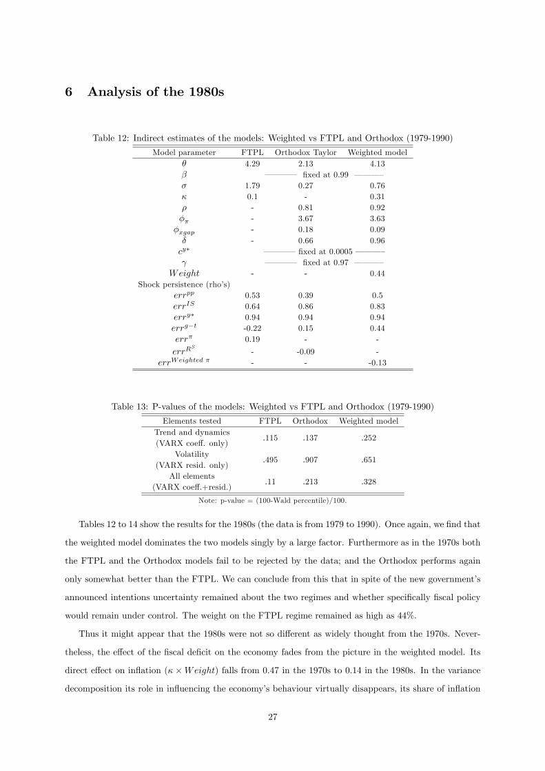
Table 12: Indirect estimates of the models: Weighted vs FTPL and Orthodox (1979-1990)

Model parameter FTPL Orthodox Taylor Weighted model� 4.29 2.13 4.13� � � � � �xed at 0.99 � � � �� 1.79 0.27 0.76� 0.1 - 0.31� - 0.81 0.92�� - 3.67 3.63�xgap - 0.18 0.09� - 0.66 0.96cy� � � � ��xed at 0.0005 � � � � � � � � �xed at 0.97 � � � �

Weight - - 0.44Shock persistence (rho�s)

errpp 0.53 0.39 0.5errIS 0.64 0.86 0.83erry� 0.94 0.94 0.94errg�t -0.22 0.15 0.44err� 0.19 - -

errRS

- -0.09 -errWeighted � - - -0.13

Table 13: P-values of the models: Weighted vs FTPL and Orthodox (1979-1990)

Elements tested FTPL Orthodox Weighted modelTrend and dynamics(VARX coe¤. only)

.115 .137 .252

Volatility(VARX resid. only)

.495 .907 .651

All elements(VARX coe¤.+resid.)

.11 .213 .328

Note: p-value = (100-Wald percentile)/100.

Tables 12 to 14 show the results for the 1980s (the data is from 1979 to 1990). Once again, we �nd that

the weighted model dominates the two models singly by a large factor. Furthermore as in the 1970s both

the FTPL and the Orthodox models fail to be rejected by the data; and the Orthodox performs again

only somewhat better than the FTPL. We can conclude from this that in spite of the new government�s

announced intentions uncertainty remained about the two regimes and whether speci�cally �scal policy

would remain under control. The weight on the FTPL regime remained as high as 44%.

Thus it might appear that the 1980s were not so di¤erent as widely thought from the 1970s. Never-

theless, the e¤ect of the �scal de�cit on the economy fades from the picture in the weighted model. Its

direct e¤ect on in�ation (� �Weight) falls from 0.47 in the 1970s to 0.14 in the 1980s. In the variance

decomposition its role in in�uencing the economy�s behaviour virtually disappears, its share of in�ation

27

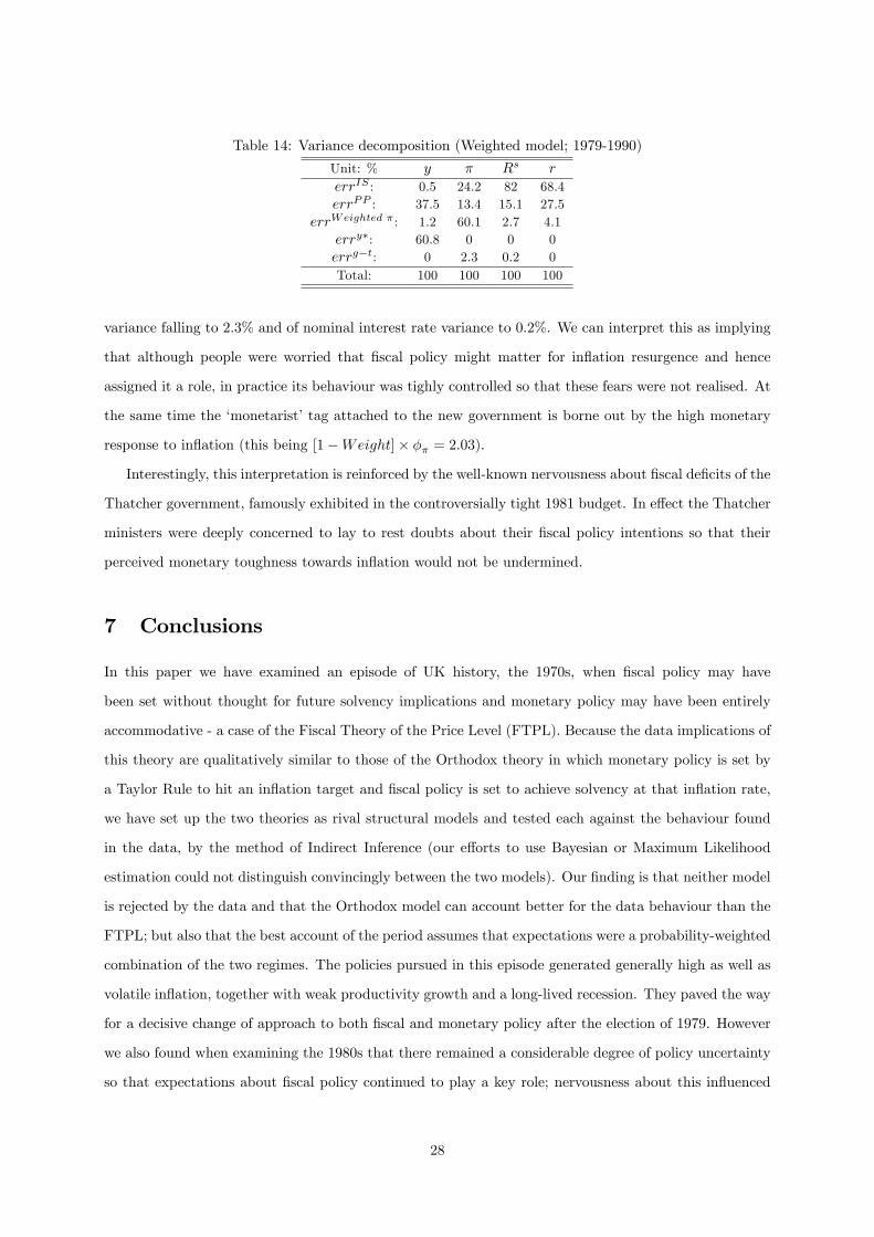
Table 14: Variance decomposition (Weighted model; 1979-1990)

Unit: % y � Rs rerrIS : 0.5 24.2 82 68.4errPP : 37.5 13.4 15.1 27.5

errWeighted � : 1.2 60.1 2.7 4.1erry�: 60.8 0 0 0errg�t: 0 2.3 0.2 0Total: 100 100 100 100

variance falling to 2.3% and of nominal interest rate variance to 0.2%. We can interpret this as implying

that although people were worried that �scal policy might matter for in�ation resurgence and hence

assigned it a role, in practice its behaviour was tighly controlled so that these fears were not realised. At

the same time the �monetarist�tag attached to the new government is borne out by the high monetary

response to in�ation (this being [1�Weight]� �� = 2:03).

Interestingly, this interpretation is reinforced by the well-known nervousness about �scal de�cits of the

Thatcher government, famously exhibited in the controversially tight 1981 budget. In e¤ect the Thatcher

ministers were deeply concerned to lay to rest doubts about their �scal policy intentions so that their

perceived monetary toughness towards in�ation would not be undermined.

7 Conclusions

In this paper we have examined an episode of UK history, the 1970s, when �scal policy may have

been set without thought for future solvency implications and monetary policy may have been entirely

accommodative - a case of the Fiscal Theory of the Price Level (FTPL). Because the data implications of

this theory are qualitatively similar to those of the Orthodox theory in which monetary policy is set by

a Taylor Rule to hit an in�ation target and �scal policy is set to achieve solvency at that in�ation rate,

we have set up the two theories as rival structural models and tested each against the behaviour found

in the data, by the method of Indirect Inference (our e¤orts to use Bayesian or Maximum Likelihood

estimation could not distinguish convincingly between the two models). Our �nding is that neither model

is rejected by the data and that the Orthodox model can account better for the data behaviour than the

FTPL; but also that the best account of the period assumes that expectations were a probability-weighted

combination of the two regimes. The policies pursued in this episode generated generally high as well as

volatile in�ation, together with weak productivity growth and a long-lived recession. They paved the way

for a decisive change of approach to both �scal and monetary policy after the election of 1979. However

we also found when examining the 1980s that there remained a considerable degree of policy uncertainty

so that expectations about �scal policy continued to play a key role; nervousness about this in�uenced

28

the Thatcher government�s policies to bring �scal de�cits down steadily so that in practice the role of

�scal policy in the economy�s behaviour was minimalised. In sum the evidence of these two decades of

UK history suggest that �scal de�cits were key to the macro-economic crises of the 1970s and bringing

them under control was important, alongside tighter monetary policy, in restoring stability in the 1980s.

References

[1] Bohn. H. (1998), �The Behaviour of U.S. Public Debt and De�cits�, Quarterly Journal of Economics,

113(3), pp949-63.

[2] Buiter, W. H. (1999), �The fallacy of the �scal theory of the price level�, CEPR discussion paper no.

2205, Centre for Economic Policy Research, London, August.

[3] Buiter, W. H. (2002), �The Fiscal Theory of the Price Level: A Critique�, The Economic Journal,

Vol. 112, pp459-480.

[4] Canova, F. (2005), �Methods for Applied Macroeconomic Research�, Princeton University Press,

Princeton.

[5] Canzoneri, M. B., Cumby, R. E. and Diba, B. T. (2001), �Is the Price Level Determined by the Needs

of Fiscal Solvency?�American Economic Review, 91 (5), pp1221-38.

[6] Carlstrom, C. T. and Fuerst, T. S. (2000), �The �scal theory of the price level�, Economic Review,

Federal Reserve Bank of Cleveland, issue Q I, pp22-32.

[7] Christiano, L. J. and Fitzgerald, T. J. (2000), �Understanding the Fiscal Theory of the Price Level,�

Economics Review, Federal Reserve Bank of Cleveland, 36(2), pp1-38.

[8] Cochrane, J. H. (1999), �A Frictionless View of U.S. In�ation�, NBER Chapters, NBER Macroeco-

nomics Annual 1998, Vol. 13, pp323-421, National Bureau of Economic Research.

[9] Cochrane, J. H. (2001), �Long Term Debt and Optimal Policy in the Fiscal Theory of the Price

Level�, Econometrica, 69(1), pp69-116.

[10] Cochrane, J. H. (2005), �Money as Stock�, Journal of Monetary Economics, Vol. 52, pp501-528.

[11] Del Negro, M & Schorfheide, S. (2006), �How good is what you�ve got? DSGE-VAR as a toolkit

for evaluating DSGE models. Economic Review, Federal Reserve Bank of Atlanta, issue Q 2, pages

21-37.

29

[12] Davig, T., Leeper, E. M. and Chung, H. (2007), �Monetary and Fiscal Policy Switching�, Journal of

Money, Credit and Banking, Vol. 39 (4), pp809-842.

[13] Gourieroux, C. and Monfort, A. (1995) �Simulation Based Econometric Methods, CORE Lectures

Series, Louvain-la-Neuve.

[14] Gourieroux, C., Monfort, A. and Renault, E. (1993), �Indirect inference�, Journal of Applied Econo-

metrics 8, pp85-118.

[15] Gregory, A. and Smith, G. (1991), �Calibration as testing: Inference in simulated macro models�,

Journal of Business and Economic Statistics Vol. 9, pp293-303.

[16] Gregory, A. and Smith, G. (1993), �Calibration in macroeconomics�, in Handbook of Statistics, G.

Maddala, ed., Vol. 11 Elsevier, St. Louis, Mo., pp703-719.

[17] Hall, R.E. (1978), �Stochastic implications of the life cycle-permanent income hypothesis: theory

and evidence�, Journal of Political Economy, 86, 971-988.

[18] Ingber, Lester (1996), �Adaptive simulated annealing (ASA): Lessons learned�, Control and Cyber-

netics, Vol. 25, pp.33

[19] Kocherlakota, N and Phelan, C. (1999), �Explaining the Fiscal Theory of the Price Level�, Federal

Reserve Bank of Minneapolis Quarterly Review, Vol. 23, No. 4 pp14-23.

[20] Le, V. P. M., Meenagh, D., Minford, P. and Wickens, M. R. (2011), �How Much Nominal Rigidity

Is There in the US Economy? Testing a New Keynesian DSGE Model Using Indirect Inference�,

Journal of Economic and Dynamic Control, Elsevier, December

[21] Le, V. P. M., Meenagh, D., Minford, P. and Wickens, M. R. (2012), �Testing DSGE models by

Indirect inference and other methods: some Monte Carlo experiments�, Cardi¤ University Working

Paper Series, E2012/15, June

[22] Le, V. P. M., Meenagh, D., Minford, P. and Wickens, M. R. (2013), �A Monte Carlo procedure for

checking identi�cation in DSGE models�, Cardi¤ University Working Paper Series, E2013/4, March.

[23] Leeper, E. (1991), �Equilibria Under Active and Passive Monetary and Fiscal Policies�, Journal of

Monetary Economics Vol. 27, pp129-147.

[24] Loyo, E. (2000), �Tight money paradox on the loose: a �scalist hyperin�ation�, mimeo, J .F. Kennedy

School of Government, Harvard University.

30

[25] McCallum, B. T. (1976), �Rational Expectations and the Natural Rate Hypothesis: some consistent

estimates�, Econometrica, Vol. 44(1), pp. 43-52, January.

[26] McCallum, B. T. (2001), �Indeterminacy, Bubbles, and the Fiscal Theory of Price Level Determina-

tion,�Journal of Monetary Economics, Vol. 47(1), pp19-30.

[27] McCallum, B. T. (2003), �Is The Fiscal Theory of the Price Level Learnable?� Scottish Journal of

Political Economy, Vol. 50, pp634-649.

[28] Meenagh, D., Minford, P. and Theodoridis, K. (2009), �Testing a model of the UK by the method

of indirect inference�, Open Economies Review, Springer, Vol. 20(2), pp. 265-291, April.

[29] Meenagh, D., Minford, P., Nowell, E., Sofat, P. and Srinivasan, N.K. (2009b), �Can the facts of UK

in�ation persistence be explained by nominal rigidity?�, Economic Modelling, Vol. 26 (5), pp978-992,

September.

[30] Meenagh, D., Minford, P. and Wickens, M. R. (2012), �Testing macroeconomic models by indirect

inference on un�ltered data�, Cardi¤ University working paper, E2012/17.

[31] Minford, P. (1980), Evidence given to Treasury and Civil Service Committee, Memorandum, in

Memoranda on Monetary Policy, HMSO 1980, Oral Evidence given in July 1980 in Committee�s

Third Report, Vol. II (Minutes of Evidence, HMSO, pp. 8-40).

[32] Minford, P (1993), �Monetary policy in the other G7 countries: the United Kingdom�, Monetary

policy in Developed Economies. (Handbook of comparative economic policies, Vol. 3, eds. M. Fratianni

and D. Salvatore), Westport, Conn. and London: Greenwood Press, pp 405�32.

[33] Nelson, E (2003), �UK Monetary Policy 1972-1997: A Guide Using Taylor Rules�, in Central Banking,

Monetary Theory and Practice: Essays in Honour of Charles Goodhart, P. Mizen (ed.) , Volume One,

Cheltenham, UK: Edward Elgar, pp.195-216.

[34] Sargent, T.J. and Wallace, N. (1981), �Some unpleasant monetary arithmetic�, Quarterly Review,

Federal Reserve Bank of Minneapolis, Fall, 1-17.

[35] Sims, C. A. (1994), �A simple model for the study of the price level and the interaction of monetary

and �scal policy�, Economic Theory, Vol. 4, pp381-399.

[36] Sims, C. A. (1997), �Fiscal Foundations of Price Stability in Open Economies�, mimeo, Yale Univer-

sity.

[37] Smets, F., Wouters, R. (2007), �Shocks and Frictions in US Business Cycles: A Bayesian DSGE

Approach�, American Economic Review, Vol. 97, pp586�606.

31

[38] Smith, A. (1993), �Estimating nonlinear time-series models using simulated vector autoregressions�,

Journal of Applied Econometrics, Vol. 8, ppS63-S84.

[39] Tanner, E. and Ramos, A.M. (2003) �Fiscal sustainability and monetary versus �scal dominance:

Evidence from Brazil, 1991-2000�, Applied Economics, Vol. 35, pp859-873.

[40] Wickens, M. R. (1982), �The E¢ cient Estimation of Econometric Models with Rational Expecta-

tions�, Review of Economic Studies, Vol. 49(1), pages 55-67, January

[41] Woodford, M. (1996), �Control of the Public Debt: A Requirement for Price Stability?�, NBER

Working Papers 5684, National Bureau of Economic Research.

[42] Woodford, M. (1998), �Doing without money: controlling in�ation in a post-monetary world�, Review

of Economic Dynamics, Vol. 1(1), p173-219.

[43] Woodford, M. (1998b), �Comment on John Cochrane, �A Frictionless View of U.S. In�ation��, in

NBER Macroeconomics Annual, Bernanke, B. and Rotemberg, J. (eds.), pp390-418.

[44] Woodford, M. (2001), �Fiscal Requirements for Price Stability�, Journal of Money, Credit and Bank-

ing�, Vol. 33(3), pp669-728.

32

AppendixA Derivation of Government Budget Constraint

The government budget constraint gives us

Bt+1

Rt= Gt � Tt +Bt + Bt

Rt

Where,

Gt is the government spending in money terms,

Tt is the government taxation in money terms,

Rt is the amount of nominal interest the government must pay. The value of the bonds outstanding

is B � 1R .

We can derive an expression for government budget constraint in the forward direction by substituting

forwards for future bonds outstanding, yields

Bt

Rt= Et

P1i=0 (Tt+i �Gt+i) 1

(1+Rt)i+1

We approximate this expression by

Bt

Rt=P1

i=0(tt�gt)(1+�t)iPt(1+ )iyt

(1+Rt)1+i

where tt; gt; �t; are the currently expected permanent values respectively of the tax/GDP and

government spending/GDP ratios, the in�ation rate, and the growth rate (assumed constant at all times);

P t; yt are respectively the permanent price level and equilibrium output

=�tt � gt

�P ty

�t

P1i=0

(1+ +�t)i

(1+Rt)1+i

=�tt � gt

�P ty

�t

P1i=0

(1+ +�t)1+i

(1+Rt)1+i(1+ +�t)

If and �t are both small enough,P1i=0

(1+ +�t)1+i

(1+Rt)1+i =

P1i=0

�1

1+Rt� ��t

�1+i=

�1

1� 11+r�

t�

� 1�=�

1r�t�

�Hence, Bt

RtP ty�t=

(tt�gt)(1+ +�t)(r�t� )

.

33