PHYSICAL REVIEW B 86, 085403 (2012)

Capture numbers and island size distributions in models of submonolayer surface growth

Martin Korner, Mario Einax,* and Philipp Maass†

Fachbereich Physik, Universitat Osnabruck, Barbarastraße 7, 49076 Osnabruck, Germany(Received 27 May 2012; published 2 August 2012)

The capture numbers entering the rate equations (RE) for submonolayer film growth are determined fromextensive kinetic Monte Carlo (KMC) simulations for simple representative growth models yielding point,compact, and fractal island morphologies. The full dependence of the capture numbers σs(�,�) on island size s

and on both the coverage � and the � = D/F ratio between the adatom diffusion coefficient D and depositionrate F is determined. Based on this information, the RE are solved to give the RE island size distribution(RE-ISD), as quantified by the number ns(�,�) of islands of size s per unit area. The RE-ISDs are shown toagree well with the corresponding KMC-ISDs for all island morphologies. For compact morphologies, however,this agreement is only present for coverages smaller than � � 5% due to a significantly increased coalescencerate compared to fractal morphologies. As found earlier, the scaled KMC-ISDs ns s

2/� as a function of scaledisland size x = s/s approach, for fixed �, a limiting curve f∞(x,�) for � → ∞. Our findings provide evidencethat the limiting curve is independent of � for point islands, while the results for compact and fractal islandmorphologies indicate a dependence on �.

DOI: 10.1103/PhysRevB.86.085403 PACS number(s): 81.15.Aa, 68.55.A−, 68.55.−a

I. INTRODUCTION

The kinetics of submonolayer nucleation and island growthduring the initial stage of epitaxial thin film growth has beenstudied intensively both experimentally and theoretically formore than three decades (for reviews, see Refs. 1–4, andreferences therein). Important aspects of the growth kineticsin the submonolayer growth regime can be described by therate equations (RE) approach.5 This approach has proven tobe very valuable in inorganic thin film growth. Interestingly,many of the theoretical concepts developed for thin film growthkinetics of inorganic materials, have shown recently to be veryvaluable also for applications in organic thin film growth.6–10

This is due to the fact that these concepts often are notspecifically referring to particular materials. Instead, they takeinto account the key mechanisms involved in the complexinterplay of deposition, evaporation, diffusion, aggregationand dissociation from a general viewpoint.

Parameters entering the RE are the capture numbersσs(�,�), which describe the strength of islands of size s tocapture adatoms at a coverage � and ratio D/F ≡ � of theadatom diffusion coefficient D and deposition flux F . Thedependence of the capture numbers on s has been studiedfor various � but only for one or a few � values. In thiswork, we present a systematic study of the full dependenceon both � and � for different types of island morphologiesand the case, where detachments of atoms from islands canbe neglected, corresponding to a critical nucleus of size i = 1.This is motivated by the following questions, which have notbeen thoroughly answered yet. (1) If the σs(�,�) are known,do the RE then predict correctly the number density ns(�,�)of islands of size s, that means the island size distribution(ISD)? This question indeed was earlier posed by Ratschand Venables11 as well as Evans et al.3 The answer to thisquestion is not obvious, since the RE with known capturenumbers σs(�,�) neglect many-particle correlation effects,12

spatial fluctuations in shapes and capture zones of islands,and coalescence events that, despite rare in the early-stagegrowth, can have a significant influence.13 (2) Is there a simple

functional form of the σs(�,�), in particular, is there a scalingof these capture numbers with respect to an effective capturelength as suggested by a self-consistent treatment14,15 basedon the RE? Do the σs , when scaled with respect to their meanσ , depend for large � on the scaled island size s/s only, assuggested by Bartelt and Evans?16

In previous studies, it has been found that the scaled ISDs2ns/� as a function of scaled island size x = s/s approaches,for fixed coverage �, a scaling function f (x) for large �.Early simulations suggested that f (x) is independent of � andmoreover not sensitive to the island morphology. However,later results showed3,16 that the morphology has an influence onthe form of f (x). In fact, one would expect the scaling functionf (x) to become independent of � if the RE with known capturenumbers correctly predict the ISD, and if the scaled capturenumbers σ/σ as a function of s/s become independent of �

for large �. Under these assumptions, an explicit relation wasproposed by Bartelt and Evans,16,17 which connects the scalingfunction of the capture numbers with the scaling function ofthe ISD. We hence address the following further questions:(3) is the scaling function f (x) independent of � for large�? What is the influence of the island morphology? Can therelation between the scaled ISD f (x) and the scaling functionfor the capture numbers be confirmed?

The RE treatment is based on a coupled set of simple rateequations describing the time evolution of the adatom densityn1 and the number density ns of islands with size s � 2, ifspatial correlations among islands during growth are neglected.Taking into account direct impingement of arriving atoms atthe border of islands, the RE for the case i = 1 read

1

F

dn1

dt= (1 − �) − 2�σ1n

21 − �n1

∑s>1

σsns − 2κ1n1

−∑s>1

κsns, (1)

1

F

dns

dt= �n1(σs−1ns−1 − σsns)

+ κs−1ns−1 − κsns , s = 2,3, . . . . (2)

085403-11098-0121/2012/86(8)/085403(11) ©2012 American Physical Society

MARTIN KORNER, MARIO EINAX, AND PHILIPP MAASS PHYSICAL REVIEW B 86, 085403 (2012)

These equations refer to the precoalescence regime whereonly adatoms are mobile and it is presumed that reevaporationof atoms and atom movements between the first and secondlayers can be disregarded. Moreover, adatoms arriving on topof an island are not counted, i.e., s in a strict sense refersto the number of substrate sites covered by an island (orthe island area). The coverage � entering Eq. (1) is givenby � = ∑

s�1 sns = 1 − exp(−F t) and takes into accountthat adatoms are generated by deposition into the uncoveredsubstrate area (as common in the literature in this field, weset the length unit equal to the the size of the substrate latticeunit). The terms with σ1(�) and κ1(�) describe the nucleationof dimers due to attachment of two adatoms by diffusion anddue to direct impingement, respectively. The term ∝ n1σsns

describes the attachment of adatoms to islands of size s > 1,and the term ∝ κsns the direct impingement of deposited atomsto boundaries of islands with size s. For the idealized pointisland model, s refers to the total number of atoms that arrivedat a point, and (1 − �) in Eq. (1) is replaced by one (nocovered substrate area). For a unified discussion of capturenumbers and the ISD, we formally set � = F t for the pointisland model.

Introducing the total number density of stable islands N

and the average capture number σ ,

N =∑s>1

ns, σ = 1

N

∑s>1

σsns, (3)

a reduced set of equations for n1(�) and N (�) can be derivedfrom Eqs. (1) and (2) within the RE treatment. These equationspredict the scaling relation N ∝ �−χ with the scaling exponentχ = 1/3.18,19 This relation has been successfully validatedby several growth experiments in the past and applied toextract adatom diffusion barriers and binding energies in metalepitaxy. A discussion of many of these experiments can befound in Ref. 2. Recently, the relation has also been appliedin organic thin film growth.6,7 An extended RE approachfor multicomponent adsorbates4,20 was recently suggested todetermine binding energies between unlike atoms from islanddensity data.21

More detailed information on the growth kinetics iscontained in the ISD. If the full dependence of the ISD ns (�,�)on � and � is mediated by the mean island size s(�,�), theISD should obey the following scaling form, as first suggestedby Vicsek and Family,22

s2(�,�)

�ns(�,�) = f

(s

s(�,�)

). (4)

Here, the scaling function f (x) must fulfill the conditions∫ ∞0 f (x)dx = ∫ ∞

0 xf (x)dx = 1. The scaling behavior wasfound to give a good effective description for large �. Moreprecisely, the curves s2ns/� as a function of x = s/s approacha limiting curve,23

lim�→∞

s2

�nxs(�,�) = f∞(x,�) . (5)

Previous studies for a few fixed � values suggest that f∞(x,�)is independent of �.

An explicit expression for the scaling function f (x) withshape independent of � was suggested by Amar and Family,24

f (x) = Cixi exp(−iaix

1/ai ). (6)

The parameters entering this scaling function depend on thesize of the critical nucleus i, which allows one to determinei in experiments.7,9,25,26 Equation (6) was believed to beindependent even of the morphology;24 but this has later beenquestioned.3,16

Based on a continuum limit of the RE (2) and scalingassumptions for the capture numbers and a neglect of the �

dependence, an expression for the limiting curve f∞(x) wasderived by Bartelt and Evans,16,17

f∞(x) = f∞(0) exp

[ ∫ x

0dy

(2z∞ − 1) − C ′tot(y)

Ctot(y) − zy

], (7)

where z∞ = ∂(ln s)/∂(ln �) and Ctot(x) is a linear combinationof the scaled capture numbers C∞(x) = σs/σ and scaled directcapture areas K∞(x) = κs/κ . The “∞” subscript indicates thatthe large � → ∞ limit should be taken. As pointed out byBartelt and Evans, Ctot(x) should be well approximated bythe scaled capture numbers alone, Ctot(x) ≈ (1 − �)C∞(x).In Appendix A, we show that in fact it holds Ctot(x) ≈C∞(x). The two conditions for f∞(x) (normalization and firstmoment equal to one) imply that C∞(0) = (1 − z)/f∞(0) and∫ ∞

0 dx C∞(x)f∞(x) = 1.3,17

It is interesting to note that a semiempirical form, which hasa structure similar to Eq. (6) has been suggested recently byPimpinelli and Einstein27 for the distribution of capture zonesA as identified by Voronoi tessellation,

Pβ = cβaβ exp(−dβa2) , (8)

where a = A/A is the rescaled capture zone with respect tothe mean A and β = i + 1 (see also Ref. 28). This distributioncorresponds to a generalized Wigner surmise from randommatrix theory. The parameter β = i + 1 and the functionalform, however, are controversially discussed.29,30

Besides this recent progress in predicting functional formsof capture zone distributions, there are only a few studies sofar13,31,32 that address the problem whether an integration ofthe REs (1) and (2) can yield correctly the ISD for differentcluster morphologies in the precoalescence regime. For anintegration of the RE, a reliable determination of σs(�,�)is needed. Four general approaches have been followed forthis purpose: (i) within a self-consistent ansatz one can solvethe diffusion field around an island and derive determiningequations for the capture numbers by equating the attachmentcurrents of the diffusion field and the RE.14,15 (ii) By modelingthe island growth with the level set method,33 one cananalogously equate attachments currents and determine thecapture numbers.31,32 (iii) Balancing the deposition rate FAsns

into the mean capture zone As of islands of size s with the REexpression Dσsn1ns for the attachment rate to these islands,yields σs � As/�n1. This means that the capture numbers canbe approximately calculated from a determination of the As ,e.g., by Voronoi tessellation.17,34–36 (iv) In simulations, wherethe individual attachments are followed, the capture numberscan be calculated from the mean number of attachments Ms toisland of size s during a time interval t [see Eq. (9) and thediscussion in Sec. II].16

085403-2

CAPTURE NUMBERS AND ISLAND SIZE DISTRIBUTIONS . . . PHYSICAL REVIEW B 86, 085403 (2012)

The paper is organized as follows. First, we describe inSec. II the method used to generate point, compact and fractalisland morphologies, and the method for determining thecapture numbers as function of island size and coverage. InSec. III, we discuss the results for the capture numbers andcompare these with the prediction of the self-consistent theory.In Sec. IV, we analyze the mean island and adatom densities forthe different island morphologies and discuss their predictionby the self-consistent RE and the RE based on the capturenumbers determined in the KMC simulations. In Sec. V,we demonstrate that the ISD is successfully predicted bythe RE as long as coalescence events can be neglected. Thesecoalescence events are relevant already for small coverages� � 0.05 for compact morphologies, while they turn out tobe much less important for fractal morphologies. The reasonfor these differences are reduced coalescence rates for fractalisland morphologies because of a screening effect.1,37 Finally,we study in Sec. VI the behavior of the scaled capture numbersand scaled ISDs in the limit � → ∞.

II. SUBMONOLAYER GROWTH: MODELS,MORPHOLOGIES AND SIMULATIONS

The KMC simulations are performed with a first reactiontime Monte Carlo algorithm38,39 on a square lattice with L × L

sites. In this algorithm, two times τF and τD are randomlygenerated from the exponential probability density ψ(τ ) =γ exp(−γ τ ), where γ = L2F for τF , corresponding to adeposition process, and γ = 4DL2n1 for τD , correspondingto one of the possible diffusive jumps of adatoms. If τD <

τF , the simulation time is incremented by τD and one ofthe L2n1 adatoms is selected randomly and moved to arandomly selected vacant nearest neighbor site. If τF < τD ,the simulation time is incremented by τF and one of the L2

sites is randomly chosen. If this site is vacant, an additionaladatom is deposited on this site, while, if the site is occupied,no deposition takes place.

With respect to the formation of islands, we considerthree simple growth models that are representative for thedifferent types of island morphologies in the case of i = 1.Fractal islands are generated by applying “hit and stick”aggregation, which means an adatom having another atom asthe nearest neighbor becomes immobilized. Compact islandmorphologies are produced by letting islands grow spirally

into a quadratic form as in Ref. 40, meaning that each adatomattached to an island is displaced to the corresponding tip of thespiral. Point island morphologies are generated by displacingan adatom attaching to an island to the site representing theisland, while bookkeeping the total number of aggregatedatoms for the island size.

To calculate the capture numbers σs at the coverage �, weuse the following procedure, which is based on the methodoutlined in Ref. 16; each simulation run is stopped at coverage� and the number densities ns = Ns/L

2, s = 1,2, . . . aredetermined, where Ns are the numbers of monomers (s = 1)and islands (s > 1). Then the simulation is continued for a timeinterval t without deposition and the following additionalrules are implemented: (i) if an adatom is attaching to anisland of size s > 1, a counter Ms is incremented and theadatom thereafter repositioned at a randomly selected site onthe free substrate area (i.e., a site which is neither covered northe nearest neighbor of a covered site), and (ii) if two adatomsform a dimer, a counter M1 is incremented and the two adatomsthereafter are repositioned randomly as described in (i). Inthis way, a stationary state is maintained at the coverage �.The mean attachment rate per unit area to islands of size s isMs/(L2t), and equating this with the expression Dσsnsn1

from the RE (1, 2) yields

σs = Ms

L2tDnsn1, s = 1,2, . . . . (9)

Averaging over many simulation runs (configurations) givesσs(�,�). The κs are determined from the lengths of the islandsboundaries, which are simultaneously monitored during thesimulation and averaged for each size s.

The continuous-time Monte Carlo (KMC) simulationsare performed on a square lattice with periodic boundaryconditions and L × L = 8000 × 8000 sites for four different� = 105, 106, 107, and 108. For each value of �, an averageover 108 nucleation/attachment events was performed.

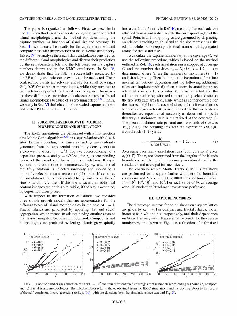
III. CAPTURE NUMBERS

The direct capture areas for point islands on a square latticeare given by κs = 4. For compact and fractal islands, the κs

increase as ∼√s and ∼s, respectively, and their dependence

on � and � is very weak. Representative results for the capturenumbers σs are shown in Fig. 1 as a function of s for fixed

0 25 50 75 100 125 150s2

2.5

3

3.5

4

4.5

σ s

Θ=0.02Θ=0.05Θ=0.10Θ=0.15

(a) point islands

0 50 100 150 200 250 300 350s0

10

20

30

σ s

Θ=0.02Θ=0.05Θ=0.10Θ=0.15

(b) compact islands

0 50 100 150 200 250 300 350s0

25

50

75

100

σ s

Θ=0.02Θ=0.05Θ=0.10Θ=0.15

(c) fractal islands

FIG. 1. Capture numbers as a function of s for � = 107 and four different fixed coverages for the models representing (a) point, (b) compact,and (c) fractal island morphologies. The filled symbols refer to the σs obtained from the KMC simulations and the open symbols to the resultsof the self-consistent theory according to Eqs. (10) (with the Rs taken from the simulations, see text and Fig. 3).

085403-3

MARTIN KORNER, MARIO EINAX, AND PHILIPP MAASS PHYSICAL REVIEW B 86, 085403 (2012)

0.01 0.1Θ

1

10

100s--- Γ=10

5

Γ=106

Γ=107

Γ=108

0 0.1 0.2Θ

1.8

2.1

2.4

2.7

3

3.3

3.6

3.9σ----

(a) point islands

0.01 0.1Θ

1

10

100

s--- Γ=105

Γ=106

Γ=107

Γ=108

0 0.1 0.2Θ

0

2

4

6

8

10

12

14σ----

(b) compact islands

0.01 0.1Θ

1

10

100

s--- Γ=105

Γ=106

Γ=107

Γ=108

0 0.1 0.2Θ

0

10

20

30

40

50

60

70σ----

(c) fractal islands

FIG. 2. Mean capture number σ and mean island size s as a function of � for the four simulated � values and the models representingpoint, compact, and fractal island morphologies.

� = 107 and four different coverages for the (a) point, (b)compact, and (c) fractal island morphologies. For the othersimulated � values, a similar behavior was obtained. The meanσ (�,�) [see Eq. (3)] as a function of � for all simulated �

values is displayed in Fig. 2, together with the mean islandsize s(�,�). These functions are later used in Sec. VI wheninvestigating the scaled capture numbers σs in connection withthe scaled island densities in the limit � → ∞.

A common feature for all morphologies in Fig. 1 is a linearincrease of σs with s for large s > s. It can be understood3

from the proportionality of the σs to the mean capture zoneareas As , and the fact that large islands typically exhibit largeAs , which led to the stronger growth of these islands. Since atwice as large capture zone gives on average rise to a twice aslarge island, it holds As ∼ s and hence σs ∝ As ∼ s.3,16

With respect to the dependence on the coverage �, theσs in Fig. 1 have a quite different behavior for the threemorphologies in the regime s > s. While for the point islandsthe σs decrease with �, they are almost independent of �

for the compact islands, and they increase with � for thefractal islands. Main reason for these differences is that forpoint islands the number density N continues to increase with� (that means time t = �/F ) due to ongoing nucleation ofnew islands, while for compact and fractal morphologies, N

tends to saturate for larger �, with less pronounced saturationin the compact case (see Sec. IV below). During the growthin the point island model, a large capture zone surroundinga large island is, compared to the other two morphologies,more frequently destroyed by a nucleation event in this zone,and the As ∝ σs thus decrease with � for fixed s > s. Dueto the higher nucleation rate and the missing spatial extensionof islands in the point island model, the corresponding σs

are much smaller than for the compact and fractal morpholo-gies. The larger island extension and the strong capture ofadatoms by finger tips in the case of fractal islands leadto about five times larger σs in comparison to the compactislands.

The differences with respect to the � dependence are alsoreflected in the behavior of σ (�,�) in Fig. 2. In fact, when con-sidering the scaled capture numbers σs/σ , the � dependencefor s > s becomes qualitatively the same for all morphologies(increase of σs/σ with �, see Sec. VI below). For small s < s,

the curves in Fig. 1 show a nonlinear dependence of σs on s

for all morphologies.35,41,42 By combining the linear functionfor large s with a polynomial at small s, we fitted the resultsfor σs for all simulated � and � values. These fits, togetherwith corresponding fits for the κs , were used to integrate theREs (1) and (2).

The mean island size s in Fig. 2 reproduces the behaviorseen in many earlier studies.3 In the point island modelthe straight lines in the double logarithmic representationare in agreement with s ∼ �z with z = 2/3 as predictedby a scaling analysis of the reduced RE.3,43,44 In the caseof the compact and fractal island morphologies, the slopez(�) = ∂ ln s(�,�)/∂ ln � increases with � and approachesz � 1 for both island morphologies. This is consistent with asaturation (�-independence) of the island density for large �

in the precoalescence regime, s ∼ �/N ∼ �.In the self-consistent theory,14 the capture numbers are

given by

σ scs = 2π

(1 − �)

Rs

ξ

K1(Rs/ξ )

K0(Rs/ξ ), (10a)

ξ−2 = 2σ sc1 n1 +

∑s�2

σ scs ns , (10b)

where Rs is the effective radius of an island of size s, K0 andK1 are the modified Bessel functions of order zero and one,respectively, and ξ is the adatom capture length (mean linearsize of depletion zone around an island). The factor (1 − �)in Eq. (10), which was not given in the original derivationin Ref. 14, arises from the fact that the adatom current toa (circular) island of size s is 2πRsD ∂r n1(r)|r=Rs

, wheren1(r) = n1(r)/(1 − �) is the adatom density with respectto the free (uncovered) surface area, and n1(r) is the localform corresponding to the global mean value n1 appearing inthe RE [see also Ref. 45 for the additional factor (1 − �)].For Rs � ξ , σs ∼ 2π/[(1 − �) ln(ξ/Rs)] and for Rs � ξ ,σs ∼ 2π/(1 − �)(Rs/ξ ).

To determine the σ scs , the REs (1) and (2) are numerically

solved with initial conditions ns = 0 at time t = 0 and a cutoffvalue sc so that ns can be safely neglected for s > sc. In eachintegration step the implicit Eq. (10) is solved for the σ sc

s .The results become sensitive to the island morphology via the

085403-4

CAPTURE NUMBERS AND ISLAND SIZE DISTRIBUTIONS . . . PHYSICAL REVIEW B 86, 085403 (2012)

100 101 102

s

100

101

Rsfractalcompact

FIG. 3. Mean radii of gyration Rs of islands of size s for themodels representing compact and fractal island morphologies. Thestraight lines in the double-logarithmic plot indicate the power-lawbehavior for large s.

dependence of Rs on s in this approach. For point islandswe take Rs = 1 corresponding to one lattice constant. For thecompact and fractal island morphologies, we determined themean radius of gyration of islands of size s, as shown in Fig. 3.The straight lines in the double-logarithmic representationgive Rs ∼ 0.42s1/2 (compact islands) and Rs ∼ 0.47s0.57

(fractal morphologies) for large s. To compare the σ scs with

the σs obtained from the KMC simulations, we used thefull dependence of the Rs on s, i.e., including the small s

behavior, in our integration of the RE. The results from theself-consistent theory are shown in Fig. 1 (open symbols). Ascan be seen from the figure, the σ sc

s deviate strongly fromthe KMC results, both in their size and in their functionalform. In particular, the self-consistent theory underestimatesthe capture numbers for large s, as known from earlier workin the literature.3

It is interesting to see, whether the scaling of (1 − �)σs(�,�) with Rs/ξ is valid, if the σs and ns from the KMCsimulations are used in the expression for ξ−2 in Eq. (10b).In this case, the linearization step used in this theory forderiving a linear diffusion equation for the local adatomdensity n1(r) could be reasoned, i.e., the step, where the term2σ1n1(r)2 + ∑

s>1 σsn1(r)ns(r) is replaced by n1(r)ξ−2 withξ−2 = 2σ1n1 + ∑

s>1 σsns given by the mean (r-independent)densities (see Ref. 14 for details). In Fig. 4, (1 − �)σs(�,�)

is plotted as a function of Rs/ξ for the models representingcompact and fractal island morphologies. Figure 4(a) showsthat indeed a data collapse is obtained for different � values atfixed �. However, with respect to the � dependence, tested inFig. 4(b), no scaling behavior is found. This indicates thatthe linearization step in the self-consistent theory leads tothe unsatisfactory capture numbers. It has been shown thatcorrelation effects between island sizes and capture areasneed to be taken into account to improve theories for capturenumbers and island size distributions. This can been achievedby considering the joint probability of island size and capturearea.42,45–48

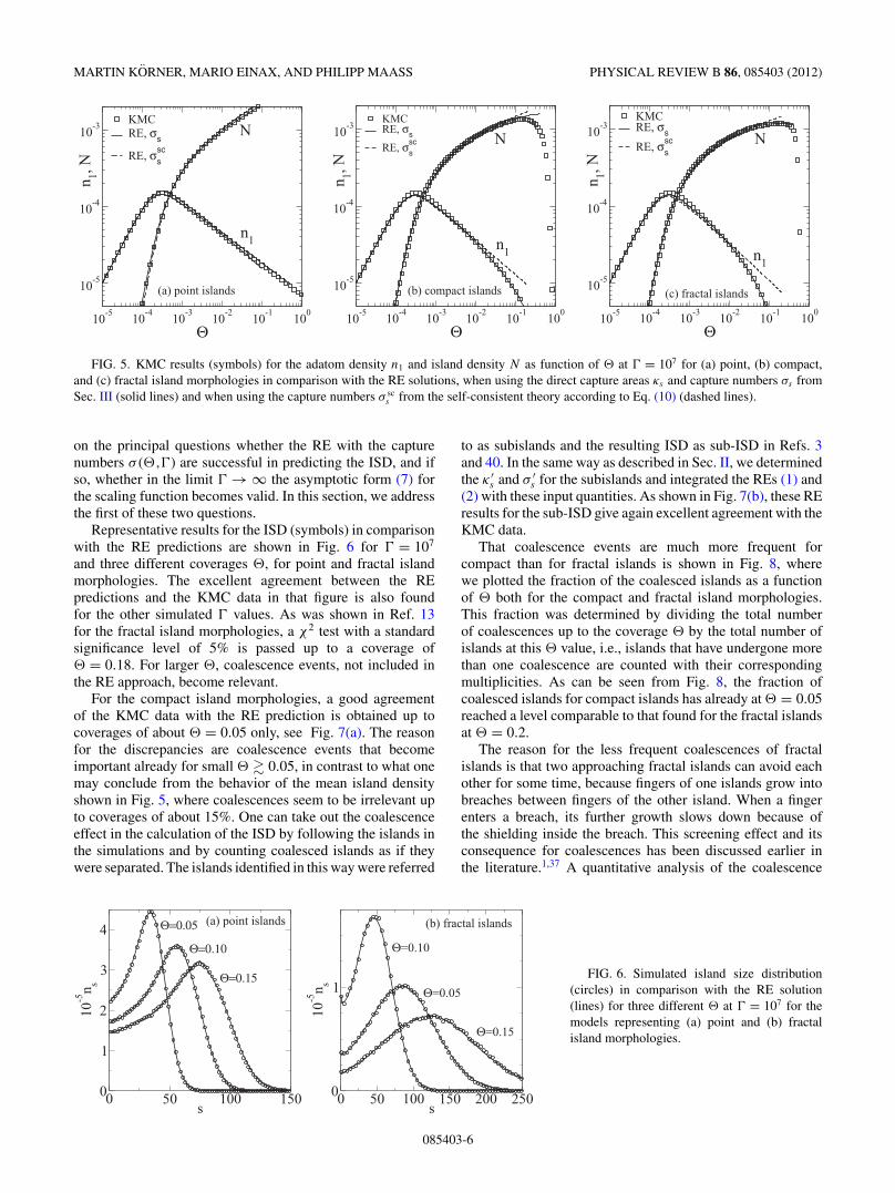
IV. ADATOM AND ISLAND DENSITIES

Numerical integration of the RE with the κs and σs fromSec. III gives an excellent description of the adatom densityn1 and of the island density N as a function of � and � forall island morphologies in the precoalescence regime. Thisis demonstrated in Fig. 5 where n1 and N from the KMCsimulation (open squares) and RE solution (solid lines) areplotted as a function of � for � = 107. For compact and fractalisland morphologies, the KMC data for N steeply fall forcoverages larger than 15% (compact islands) and 30% (fractalislands) because of island coalescences. Small deviations of theRE solution for n1 can be seen close to its maximum, where itslightly underestimates the adatom density. The agreement forthe other simulated � values is of the same quality. As knownfrom previous studies,1,11,14,45 the RE predict n1 and N quitewell also, when using the self-consistent capture numbers fromEq. (10). The corresponding solutions are drawn as dashedlines in Fig. 5. In view of the discrepancies discussed in Sec. III,this good predictive power of the RE under use of the self-consistent capture numbers σ sc

s is surprising.

V. ISLAND SIZE DISTRIBUTIONS

Since the σ scs (�,�) deviate strongly from the σs(�,�),

the RE with self-consistent capture numbers fail to predict theISD. This failure was reported already when the self-consistingtheory was developed.14 In the following, we therefore dono longer consider the self-consistent theory, but concentrate

0 0.2 0.4 0.6 0.8Rs/ξ

0

5

10

15

20

25

30

35

(1-Θ

)σs

Γ=105

Γ=106

Γ=107

Γ=108

0 1 2 3Rs/ξ

0

50

(1-Θ

)σs

compact islands

fractal islands (a)

0 0.2 0.4 0.6 0.8Rs/ξ

0

5

10

15

20

25

30

35

(1-Θ

)σs

Θ=0.02Θ=0.05Θ=0.10Θ=0.15

0 1 2 3Rs/ξ

0

50

(1-Θ

)σs

compact islands

fractal islands (b)

FIG. 4. Scaling plot of (1 − �)σs as a function of Rs/ξ for the model representing compact island morphologies, with both Rs andξ−2 = 2σ1n1 + ∑

s�2 σsns determined from the KMC simulations, (a) for various � and fixed � = 0.2 and (b) for various � and fixed� = 108. The insets in (a) and (b) show the corresponding results for the model representing fractal island morphologies. The solid linesrepresent the specific functional form in Eq. (10) predicted by the self-consistent theory.

085403-5

MARTIN KORNER, MARIO EINAX, AND PHILIPP MAASS PHYSICAL REVIEW B 86, 085403 (2012)

10-5

10-4

10-3

10-2

10-1

100

Θ

10-5

10-4

10-3

n 1, N

KMCRE, σs

RE, σssc N

n1

(b) compact islands

10-5

10-4

10-3

10-2

10-1

100

Θ

10-5

10-4

10-3

n 1, N

KMCRE, σs

RE, σssc N

n1

(c) fractal islands

10-5

10-4

10-3

10-2

10-1

100

Θ

10-5

10-4

10-3

n 1, N

KMCRE, σs

RE, σssc

N

n1

(a) point islands

FIG. 5. KMC results (symbols) for the adatom density n1 and island density N as function of � at � = 107 for (a) point, (b) compact,and (c) fractal island morphologies in comparison with the RE solutions, when using the direct capture areas κs and capture numbers σs fromSec. III (solid lines) and when using the capture numbers σ sc

s from the self-consistent theory according to Eq. (10) (dashed lines).

on the principal questions whether the RE with the capturenumbers σ (�,�) are successful in predicting the ISD, and ifso, whether in the limit � → ∞ the asymptotic form (7) forthe scaling function becomes valid. In this section, we addressthe first of these two questions.

Representative results for the ISD (symbols) in comparisonwith the RE predictions are shown in Fig. 6 for � = 107

and three different coverages �, for point and fractal islandmorphologies. The excellent agreement between the REpredictions and the KMC data in that figure is also foundfor the other simulated � values. As was shown in Ref. 13for the fractal island morphologies, a χ2 test with a standardsignificance level of 5% is passed up to a coverage of� = 0.18. For larger �, coalescence events, not included inthe RE approach, become relevant.

For the compact island morphologies, a good agreementof the KMC data with the RE prediction is obtained up tocoverages of about � = 0.05 only, see Fig. 7(a). The reasonfor the discrepancies are coalescence events that becomeimportant already for small � � 0.05, in contrast to what onemay conclude from the behavior of the mean island densityshown in Fig. 5, where coalescences seem to be irrelevant upto coverages of about 15%. One can take out the coalescenceeffect in the calculation of the ISD by following the islands inthe simulations and by counting coalesced islands as if theywere separated. The islands identified in this way were referred

to as subislands and the resulting ISD as sub-ISD in Refs. 3and 40. In the same way as described in Sec. II, we determinedthe κ ′

s and σ ′s for the subislands and integrated the REs (1) and

(2) with these input quantities. As shown in Fig. 7(b), these REresults for the sub-ISD give again excellent agreement with theKMC data.

That coalescence events are much more frequent forcompact than for fractal islands is shown in Fig. 8, wherewe plotted the fraction of the coalesced islands as a functionof � both for the compact and fractal island morphologies.This fraction was determined by dividing the total numberof coalescences up to the coverage � by the total number ofislands at this � value, i.e., islands that have undergone morethan one coalescence are counted with their correspondingmultiplicities. As can be seen from Fig. 8, the fraction ofcoalesced islands for compact islands has already at � = 0.05reached a level comparable to that found for the fractal islandsat � = 0.2.

The reason for the less frequent coalescences of fractalislands is that two approaching fractal islands can avoid eachother for some time, because fingers of one islands grow intobreaches between fingers of the other island. When a fingerenters a breach, its further growth slows down because ofthe shielding inside the breach. This screening effect and itsconsequence for coalescences has been discussed earlier inthe literature.1,37 A quantitative analysis of the coalescence

0 50 100 150s0

1

2

3

4

10-5

n s

Θ=0.05

Θ=0.10

Θ=0.15

(a) point islands

0 50 100 150 200 250s0

1

10-5

n s

Θ=0.05

Θ=0.10

Θ=0.15

(b) fractal islands

FIG. 6. Simulated island size distribution(circles) in comparison with the RE solution(lines) for three different � at � = 107 for themodels representing (a) point and (b) fractalisland morphologies.

085403-6

CAPTURE NUMBERS AND ISLAND SIZE DISTRIBUTIONS . . . PHYSICAL REVIEW B 86, 085403 (2012)

0 50 100 150 200s0

1

2

10-5

n s

(a) Θ=0.05

Θ=0.10

Θ=0.15

0 50 100 150 200s0

1

2

10-5

n s

(b) Θ=0.05

Θ=0.10

Θ=0.15

FIG. 7. (a) ISD and (b) sub-ISD for compactislands obtained from the KMC simulations(circles) in comparison with the RE solution(lines) for � = 107 and three different coverages�.

behavior of compact and fractal island morphologies is givenin Appendix B.

VI. LIMITING BEHAVIOR FOR � → ∞Based on our first key finding that for all morphologies and

for all coverages in the pre-coalescence regime, the ISDs fromthe KMC simulations are successfully predicted by the RE wenow turn to the question, whether the scaled ISDs approachthe asymptotic form (7) in the limit � → ∞.

To answer this question is not easy because of varioussubtleties, which let us revisit the derivation of the scalingfunction by Bartelt and Evans16,17 in Appendix A. Asmentioned in Introduction, Eq. (4) for the limiting curveof the scaled ISD f∞(x) should be valid if f∞(x,�)from Eq. (5) is independent of �. This is the case ifC∞(x,�) = lim�→∞ σxs(�,�)/σ (�,�) for the scaledcapture numbers and z∞(�) = lim�→∞ ∂ ln s(�,�)/∂ ln �

also have �-independent limits. A further requirement for thevalidity of Eq. (7) is that lim�→∞ κ(�,�)/s(�,�) = 0, whereκ = N−1 ∑

s>1 κsns is the mean direct capture area. Thiscondition can be expected to be fulfilled for compact and pointisland morphologies and is in fact the reason, why the scalingfunction of the direct capture areas should not enter the REprediction (7). If lim�→∞ κ(�,�)/s(�,�) > 0, f∞(x,�) canbe expected to depend on � and one would need to solve thesemi-linear partial differential equation (A6) for f∞(x,�).Note that the κs cannot increase stronger than linearly withs, and accordingly κ should not increase more than linearlywith s.

0 0.05 0.1 0.15 0.2Θ

10-4

10-3

10-2

10-1

frac

tion

of c

oale

sced

isla

nds compact islands

fractal islands

FIG. 8. Fraction of coalesced islands as a function of the coverage� for � = 107.

In interpreting numerical results for finite �, we have topay attention to the fact that for smaller � larger � valuesare needed to approach the limiting curves. This is becauses(�,�) must become large enough to reach the “continuumlimit” (and larger � are needed to obtain the same s at smaller�), and because the relation n1 ∼ (1 − �)/�σN , used in thederivation of Eq. (7), should be obeyed. This relation is usuallyreferred to as the quasistationary condition, since it followsfrom balancing the adatom attachment rate DσnN to islandswith the deposition rate F (1 − �). However, as was shownearlier,44 the relation is also valid for small � values in theregimes, where relative changes of N are still large and havenot leveled off. A refined scaling analysis yields that, for i = 1as relevant here, the relation holds for (�2�)1/3 � 1, implyingagain that for smaller � larger � are needed to identify thelimiting behavior.

Figure 9 shows ns s2/� as a function of s/s for � = 108 at

four different coverages for the (a) point and (b) fractal islandmorphologies. In the insets, the scaled ISDs are shown fora fixed coverage � = 0.2 and different �. In the case of thepoint island morphologies, the data suggest the existence ofa �-independent limiting curve, in agreement with previousfindings.3 For the fractal island morphologies, the scaled ISDfor different � show no clear signature of a �-independentlimiting curve. Based on the tendency of the simulated datafor different � and � to become slightly closer to eachother for larger � and �, one may conjecture that also inthis case a limiting curve would be reached at larger �

values. However, the fact that for each fixed �, the curvesat large � are almost overlapping suggests that these aregood estimates of f∞(x,�). Our conclusion is therefore thatit is not likely that a �-independent limiting curve existsfor the hit-and-stick model used here for the fractal islandmorphologies.

This conclusion is further corroborated by the fact thatthe scaled direct capture areas exhibit a nearly linear de-pendence on x for the fractal islands (not shown). Thus weencounter the case here, where the scaled direct capture areasκ(�,�)/s(�,�) appear to approach a non-vanishing limitfor � → ∞, which would mean that in a strict treatment,Eq. (7) can no longer be applied. If one considers f∞(x,�) todepend only very weakly on �, ∂f∞(x,�)/∂� � 0, we couldreplace C∞(x) by Ctot(x) = C∞(x) + ρ∞�K∞(x,�)/(1 −�), where K∞(x,�) = lim�→∞ κxs(�,�)/κ(�,�) is the lim-iting curve for the scaled direct capture areas and ρ∞ =lim�→∞ κ(�,�)/s(�,�) > 0.

085403-7

MARTIN KORNER, MARIO EINAX, AND PHILIPP MAASS PHYSICAL REVIEW B 86, 085403 (2012)

0 0.5 1 1.5 2 2.5s/s

10-2

10-1

100

n ss2 /Θ

Θ=0.02Θ=0.05Θ=0.10Θ=0.20

0 1 2s/s10-2

10-1

n ss2 /Θ

Γ=105

Γ=106

Γ=107

Γ=108

(a) point islands

Θ=0.2

Γ=108

0 0.5 1 1.5 2 2.5s/s

10-2

10-1

100

n ss2 /Θ

Θ=0.02Θ=0.05Θ=0.10Θ=0.20

0 1 2s/s10-2

10-1

n ss2 /Θ

Γ=105

Γ=106

Γ=107

Γ=108

(b) fractal islands

Γ=108

Θ=0.2

FIG. 9. Scaled island size distributions ns s2/� as function of the scaled island size x = s/s for fixed � = 108 and four coverages �, for

(a) point and (b) fractal island morphologies. The insets show the scaled ISDs at fixed � = 0.2 and the four simulated � values. The line in (a)is a fit to the data for � = 0.2 and � = 108 and agrees with the analytical result Eq. (7), when using the line in Fig. 10(a) as the estimate forC∞(x).

Our conclusions drawn with respect to the scaled ISDs ofthe point islands are consistent with the behavior of the scaledcapture numbers, which are shown in Fig. 10(a) for the same �

and � values as in Fig. 9(a). In this Fig. 10(a), an approach to a�-independent limiting curve C∞(x) can be seen. In the caseof the fractal island morphologies by contrast, an approach toa �-independent limiting curve cannot be clearly identified,which gives further evidence that the f∞(x,�) are dependenton �.

In order to test the validity of Eq. (7) for the point islands,we set z∞ = 2/3 (see Sec. III) and used a fit to the scaledISD for � = 108 and � = 0.2 in Fig. 9(a) as an estimate forf∞(x). The fit, which fulfills the constraints of normalizationand normalized first moment, is shown as line in this figure. Wethen estimated C∞(x) based on this fit by rewriting Eq. (A6)from Appendix A [for �-independent f∞(x)] in the form

dC∞(x)

dx= (2z∞ − 1) − [C∞(x) − z∞x]

d ln[f∞(x)]

dx. (11)

Since the solution of this differential equation is proportionalto 1/f∞(x), we preferred to integrate Eq. (11) with theinitial condition C∞(0) = f∞(0)/(1 − z∞) to achieve a stablenumerical results for large x also. The resulting estimate forC∞(x) is shown as line in Fig. 10(a). The line lies slightlyabove the data for the scaled capture numbers for � = 108 and

� = 0.2, indicating that indeed an estimate of a limiting curvefor the scaled capture numbers is obtained. In a cross check,we performed the integral in Eq. (7) with the estimated C∞(x)and recovered the line in Fig. 9(a).

For the compact island morphologies, Eq. (7) would beof limited practical use, because, as discussed in Sec. V, theREs (1) and (2) fail to predict the ISD correctly already atsmall � due to coalescences. Nevertheless, from a conceptualviewpoint, it is interesting to study the scaled ISD and theirrelation to the scaled capture numbers for the subislands. Thecorresponding data shown in Fig. 11 indicate a behavior similaras for the fractal island morphologies, where the limitingcurves are dependent on �.

VII. SUMMARY

The capture numbers entering the RE for the growth kineticsof thin films have been determined by KMC simulations intheir dependence on both the coverage � and the � = D/F

ratio for the point island model and for two simple growthmodels representative for islands with compact and fractalshapes. It was shown that the � dependence of the capturenumbers could not be accounted for by the ratio Rs/ξ ofthe mean island radius Rs and the effective adatom capturelength ξ of the RE. This suggests that the strong deviations

0 0.5 1 1.5 2 2.5s/s

0.8

1

1.2

1.4

1.6

1.8

σ s/σ

Θ=0.02Θ=0.05Θ=0.10Θ=0.20

0 1 2 3s/s

1

1.5

σ s/σ

Γ=105

Γ=106

Γ=107

Γ=108

(a) point islands

Θ=0.2

0 0.5 1 1.5 2 2.5 3s/s

0

0.5

1

1.5

2

2.5

3

σ s/σ

Θ=0.02Θ=0.05Θ=0.10Θ=0.20

0 1 2s/s0

1

2

3

σ s/σ

Γ=105

Γ=106

Γ=107

Γ=108

(b) fractal islands

Θ=0.2

Γ=108

FIG. 10. Scaled capture numbers σs/σ as function of the scaled island size s/s for fixed � = 108 and four coverages �, for (a) point and(b) fractal island morphologies. The insets show the scaled capture numbers at fixed � = 0.2 and the four simulated � values. The line in(a) marks the solution obtained from a numerical integration of Eq. (11) when using the fit (line) to the scaled ISDs curve for � = 108 and� = 0.2 in Fig. 9(a).

085403-8

CAPTURE NUMBERS AND ISLAND SIZE DISTRIBUTIONS . . . PHYSICAL REVIEW B 86, 085403 (2012)

0 0.5 1 1.5 2 2.5s/s

10-2

10-1

100

n ss2 /Θ

Θ=0.02Θ=0.05Θ=0.10Θ=0.20

0 1 2s/s10-2

10-1

n ss2 /Θ

Γ=105

Γ=106

Γ=107

Γ=108

Γ=108

Θ=0.2

(a)

Γ=108

Θ=0.2

0 0.5 1 1.5 2 2.5s/s

0

0.5

1

1.5

2

2.5

σ s/σ

Θ=0.02Θ=0.05Θ=0.10Θ=0.20

0 1 2s/s0

1

2

σ s/σ

Γ=105

Γ=106

Γ=107

Γ=108

(b)

Θ=0.2

Γ=108

FIG. 11. (a) Scaled island size distributions and (b) scaled capture numbers of subislands as function of the scaled island size in the case ofcompact island morphologies for fixed � = 108 and four coverages �. The inset shows the corresponding data at fixed � = 0.2 and the foursimulated � values.

between the capture numbers determined from the simulationsand the ones predicted by the self-consistent theory have theirorigin in the linearization step used in this theory. The REwith self-consistent capture numbers nevertheless provide agood quantitative account of the adatom and island density.The deviations to the correct capture numbers lead, however,to a failure for a description of the ISD.

Integration of the RE with the simulated capture numbersdetermined from the KMC simulations gives an excellentquantitative prediction of the ISDs. For the compact islandsmorphologies, it was found that coalescence events, notconsidered in the RE, become relevant already at small cover-ages well below � � 0.15, where coalescence events do notsignificantly affect the island density. Compared to the fractalisland morphologies, the coalescence rate for the compactmorphologies is much higher. The ISD is affected alreadyby a rather small number of coalescences, because these leadto a reshuffling of weights for different island sizes. The lowercoalescence rate for fractal morphologies is caused by thefact that fingers of two approaching fractal islands typicallyfirst avoid each other, which subsequently leads to a screeningeffect and a slowing down of further growth of these fingers.

Finally, we discussed the limiting curves for the scaledISDs when � → ∞. For the point islands the KMC dataprovide evidence that these limiting curves are independentof the coverage, which is given by the RE prediction (7). Thismeans that there exists a true scaling behavior in the � → ∞limit, where the dependence on � is fully accounted for bythe mean island size s. For the growth models representingcompact and fractal island morphologies, the results indicatethat the limiting curves are dependent on �. This impliesthat one needs to solve the partial differential equation(A6) [or Eq. (A10)] to calculate f∞(x,�) from C∞(x,�).Unfortunately, no successful theory exists so far to predict thelimiting curve C∞(x,�) for the scaled capture numbers.

The limiting curves are also different for different mor-phologies. Considering how sensitive the shape of the limitingcurves depends on the nonlinear behavior of the scaled capturenumbers as a function of the scaled island size, it is wellpossible that the shape will also vary with details of the growthmechanisms, even if the type of island morphology remainsessentially the same.

APPENDIX A: RATE EQUATION PREDICTIONOF THE LIMITING CURVES FOR THE SCALED

ISLAND SIZE DISTRIBUTION

For large �, s ∼ N−1 ∼ �1/3 and x = s/s becomes acontinuous variable, which allows one to derive a determiningequation for the scaled ISD in dependence of the scaled capturenumbers. The derivation was first presented by Bartelt andEvans.16,17 Replacing the variable s by x and using ∂/∂(F t) =(1 − �)∂/∂�, Eq. (2) can be written in the continuum limit as

∂nxs

∂�= − 1

(1 − �)s

[�n1

∂

∂x(σxsnxs) + ∂

∂x(κxsnxs)

]. (A1)

Defining f (x,�,�) = s2nxs/�, C(x,�,�) = σxs/σ , andK(x,�,�) = κxs/κ , one has

∂

∂x(σxsnxs) = �σ

s2

∂(Cf )

∂x, (A2)

∂

∂x(κxsnxs) = �κ

s2

∂(Kf )

∂x(A3)

∂nxs

∂�= −(2z − 1)f − zx

∂f

∂x+ �

∂f

∂�, (A4)

where z(�,�) = ∂ ln s/∂ ln �. The reduced RE moreoverpredict n1 ∼ (1 − �)/(�σN ) ∼ (1 − �)s/(��σ ) for large� and fixed � > �x ∼ �−1/2. Inserting this relation andEqs. (A2)–(A4) into Eq. (A1) gives

(2z − 1)f + zx∂f

∂x− �

∂f

∂�= ∂(Cf )

∂x+ �κ

(1 − �)s

∂(Kf )

∂x.

(A5)

Introducing the limits C∞(x,�) = lim�→∞ C(x,�,�),K∞(x,�) = lim�→∞ K(x,�,�) and z∞(�) = lim�→∞z(�,�), Eq. (A5) yields a determining equation forf∞(x,�) = lim�→∞ f (x,�,�).

For lim�→∞ κ/s = 0, one obtains

(2z∞ − 1)f∞ + z∞x∂f∞∂x

− �∂f∞∂�

= ∂(C∞f∞)

∂x. (A6)

The condition lim�→∞ κ/s = 0 is valid for point islands, and itcan be expected to hold also for compact island morphologiesunless atoms deposited on top of islands are essentially allattaching to the island edge in the first layer (a situationunlikely due to second layer nucleation on larger islands).

085403-9

MARTIN KORNER, MARIO EINAX, AND PHILIPP MAASS PHYSICAL REVIEW B 86, 085403 (2012)

When integrating Eq. (A6) over x from zero to infinity, thefirst, second, and third terms on the left-hand side yield (2z∞ −1), z∞ (after a partial integration) and zero, respectively,because of the normalization of f∞. The right-hand sidebecomes [−C∞(0,�)f∞(0,�)] (note that for large x, C∞ ∼ x,and f∞ must decrease faster than x to be normalizable—simulation results show that f∞ should in fact decay muchfaster). Accordingly, the relation

f∞(0,�) = 1 − z∞(�)

C∞(0,�)(A7)

must be fulfilled. A corresponding relation can be derived inthe same way already from Eq. (A5). Analogously, when firstmultiplying Eq. (A6) with x and then integrating, one obtains∫ ∞

0C∞(x,�)f∞(x,�) = 1 . (A8)

Integrating Eq. (A6) to a finite value x then yields

C∞(x,�) = z∞(�)x + 1 − z∞(�)

f∞(x,�)

∫ ∞

x

dx ′ f∞(x ′,�)

− �

f∞(x,�)

∂

∂�

∫ x

0dx ′ f∞(x ′,�) , (A9)

which expresses C∞(x,�) as a functional of f∞(x,�).When one further assumes that the limiting curve f∞ is

independent of �, one has ∂f∞/∂� = 0 and can neglect thecorresponding term in Eq. (A5). For self-consistency, thisrequires also C∞ and z∞ to become independent of �. In fact,one can conversely show that if C∞ and z∞ are independent of�, f∞ must by independent of � also. Under this assumptionEq. (A6) then reduces to a separable ordinary differentialequation, whose solution is given by Eq. (7), with Ctot(x)equal to C∞(x) and z equal to z∞.

If there exists a finite limit ρ∞(�) = lim�→∞ κ/s > 0, asit may be the case for fractal island morphologies (see thediscussion in Sec. VI), Eq. (A5) yields

(2z∞ − 1)f∞ + z∞x∂f∞∂x

− �∂f∞∂�

= ∂(C∞f∞)

∂x+ ρ∞

�

(1 − �)

∂(K∞f∞)

∂x(A10)

as determining equation for f∞(x,�). Strictly speaking, a�-independent f∞(x) should not exist then, and one needsto solve the semilinear partial differential equation (A10).If one nevertheless makes the approximation ∂f∞/∂� � 0in Eq. (A10) and considers C∞ and z∞ to be independent

of (or only weakly dependent on) �, one would obtainthe weakly �-dependent solution Eq. (7) with Ctot = C∞ +ρ∞�K∞/(1 − �).

APPENDIX B: QUANTITATIVE ANALYSIS OFCOALESCENCE EVENTS

For a quantitative analysis of the coalescence behavior, wedetermined the fraction of pair distance vectors of coalescingislands that before coalescence exhibit an antiparallel orien-tation to the vector connecting the center of masses of theislands. Let us denote by Ri,j the vector pointing from thecenter of mass of island i to the center of mass of island j , andby riα,jβ the vector pointing from atom α of island i to atom β

of island j . The fraction of distance vectors with antiparallelorientation then is

�ij = 1

sisj

∑α,β

H (−riα,jβ · Ri,j ) , (B1)

where H (.) is the Heaviside jump function with H (x) = 1for x > 0 and zero else. For a given time lag t beforecoalescence, the �ij were averaged over all coalescenceevents, yielding the mean fraction �(t) of distance vectorswith anti-parallel orientation. To obtain the correspondingdata, configurations generated by the KMC simulations wereanalyzed afterwards back in time, starting from the instantwhere islands first touched each other.

The mean fraction � obtained from this analysis isshown in Fig. 12(a) as a function of t for � = 107. Weassigned negative values to t to emphasize that �(t)was determined for lags before a coalescence event. That�(t) for fractal islands is by many orders of magnitudelarger than for compact islands demonstrates the partialinter-penetration of the fractal islands before coalescence.The value �(t) � 0.01 reached for the fractal islandmorphologies in the limit t → 0 means that on averageabout 10% of the atoms of each island in a coalescenceevent pass each other. That the partial inter-penetration isaccompanied by a slowing down of the approach of twoislands before coalescence can be seen in Fig. 12(b), where theaveraged minimal distance d(t) between coalescing islandsis shown, that means dij = minα,β(|riα,jβ |) averaged over allcoalescences of islands i and j for time lag t . The (negative)slope of d(t) is significantly smaller for the fractal islandmorphologies, giving evidence for the screening effect.1,37

-0.12 -0.09 -0.06 -0.03 0Δt

10-5

10-4

10-3

10-2

Φ

fractal islandscompact islands

(a)

-0.09 -0.06 -0.03 0Δt

2

3

4

5d

fractal islandscompact islands

(b)

FIG. 12. (a) Mean fraction � of distancevectors with antiparallel orientation (with re-spect to the center of mass distance vector)and (b) mean minimal distance d betweenislands as a function of the time lag t < 0before a coalescence event at zero time. Thetimes are given in units of F −1 and the datawere determined from the KMC simulations for� = 107.

085403-10

CAPTURE NUMBERS AND ISLAND SIZE DISTRIBUTIONS . . . PHYSICAL REVIEW B 86, 085403 (2012)

*mario.einax@uni-osnabrueck.de†philipp.maass@uni-osnabrueck.de;http://www.statphys.uni-osnabrueck.de1H. Brune, Surf. Sci. Rep. 31, 125 (1998).2T. Michely and J. Krug, Islands, Mounds and Atoms: Patterns andProcesses in Crystal Growth far from equilibrium (Springer, Berlin,2004).

3J. W. Evans, P. A. Thiel, and M. C. Bartelt, Surf. Sci. Rep. 61, 1(2006).

4W. Dieterich, M. Einax, and P. Maass, Eur. Phys. J. Special Topics161, 151 (2008).

5J. A. Venables, Phil. Mag. 27, 697 (1973).6G. Hlawacek, P. Puschnig, P. Frank, A. Winkler, C. Ambrosch-Draxl, and C. Teichert, Science 321, 108 (2008).

7F. Loske, J. Lubbe, J. Schutte, M. Reichling, and A. Kuhnle, Phys.Rev. B 82, 155428 (2010).

8A. Zangwill and D. D. Vvedensky, Nano Lett. 11, 2092 (2011).9T. Potocar, S. Lorbek, D. Nabok, Q. Shen, L. Tumbek, G. Hlawacek,P. Puschnig, C. Ambrosch-Draxl, C. Teichert, and A. Winkler, Phys.Rev. B 83, 075423 (2011).

10M. Korner, F. Loske, M. Einax, A. Kuhnle, M. Reichling, andP. Maass, Phys. Rev. Lett. 107, 016101 (2011).

11C. Ratsch and J. A. Venables, J. Vac. Sci. Technol. A 21, S96 (2003).12When starting from a many-particle master equation for the growth

kinetics of interacting adsorbate particles, the nonlinear terms inthe rate equations would arise from some mean-field treatment ofhigher order correlation functions of occupations numbers, see, forexample, J.-F. Gouyet et al., Adv. Phys. 52, 523 (2003).

13M. Korner, M. Einax, and P. Maass, Phys. Rev. B 82, 201401(2010).

14G. S. Bales and D. C. Chrzan, Phys. Rev. B 50, 6057 (1994).15G. S. Bales and A. Zangwill, Phys. Rev. B 55, R1973 (1997).16M. C. Bartelt and J. W. Evans, Phys. Rev. B 54, R17359 (1996).17J. W. Evans and M. C. Bartelt, Phys. Rev. B 63, 235408 (2001).18J. A. Venables, G. D. T. Spiller, and M. Hanbucken, Rep. Prog.

Phys. 47, 399 (1984).19J. A. Venables, Surf. Sci. 299–300, 798 (1994).20M. Einax, S. Ziehm, W. Dieterich, and P. Maass, Phys. Rev. Lett.

99, 016106 (2007).21M. Einax, W. Dieterich, and P. Maass, J. Appl. Phys. 105, 054312

(2009).22T. Vicsek and F. Family, Phys. Rev. Lett. 52, 1669 (1984).23D. D. Vvedensky, Phys. Rev. B 62, 15435 (2000).

24J. G. Amar and F. Family, Phys. Rev. Lett. 74, 2066 (1995).25R. Ruiz, B. Nickel, N. Koch, L. C. Feldman, R. F. Haglund, A. Kahn,

F. Family, and G. Scoles, Phys. Rev. Lett. 91, 136102 (2003).26J. M. Pomeroy and J. D. Brock, Phys. Rev. B 73, 245405 (2006).27A. Pimpinelli and T. L. Einstein, Phys. Rev. Lett. 99, 226102 (2007).28T. J. Oliveira and F. D. A. Aarao, Reis, Phys. Rev. B 83, 201405

(2011).29M. Li, Y. Han, and J. W. Evans, Phys. Rev. Lett. 104, 149601 (2010).30A. Pimpinelli and T. L. Einstein, Phys. Rev. Lett. 104, 149602

(2010).31F. G. Gibou, C. Ratsch, M. F. Gyure, S. Chen, and R. E. Caflisch,

Phys. Rev. B 63, 115401 (2001).32F. Gibou, C. Ratsch, and R. Caflisch, Phys. Rev. B 67, 155403

(2003).33M. F. Gyure, C. Ratsch, B. Merriman, R. E. Caflisch, S. Osher,

J. J. Zinck, and D. D. Vvedensky, Phys. Rev. E 58, R6927 (1998).34M. C. Bartelt, C. R. Stoldt, C. J. Jenks, P. A. Thiel, and J. W. Evans,

Phys. Rev. B 59, 3125 (1999).35M. C. Bartelt, A. K. Schmid, J. W. Evans, and R. Q. Hwang, Phys.

Rev. Lett. 81, 1901 (1998).36J. B. Hannon, M. C. Bartelt, N. C. Bartelt, and G. L. Kellogg, Phys.

Rev. Lett. 81, 4676 (1998).37H. Brune, G. S. Bales, J. Jacobsen, C. Boragno, and K. Kern, Phys.

Rev. B 60, 5991 (1999).38V. Holubec, P. Chvosta, M. Einax, and P. Maass, Europhys. Lett.

93, 40003 (2011).39D. T. Gillespie, J. Phys. Chem. 81, 2340 (1977).40M. C. Bartelt and J. W. Evans, Surf. Sci. 298, 421 (1993).41M. C. Bartelt, C. R. Stoldt, C. J. Jenks, P. A. Thiel, and J. W. Evans,

Phys. Rev. B 59, 3125 (1999).42J. G. Amar, M. N. Popescu, and F. Family, Phys. Rev. Lett. 86, 3092

(2001).43M. C. Bartelt and J. W. Evans, Phys. Rev. B 46, 12675 (1992).44W. Dieterich, M. Einax, S. Heinrichs, and P. Maass, Fluctuation

effects in kinetic thin film growth, in Anomalous FluctuationPhenomena in Complex Systems: Plasmas, Fluids, and FinancialMarkets, edited by C. Riccardi and H. E. Roman (TransworldResearch Network, Kerala, India, 2008), Chap. 8, pp. 211–244.

45M. N. Popescu, J. G. Amar, and F. Family, Phys. Rev. B 64, 205404(2001).

46P. A. Mulheran and D. A. Robbie, Europhys. Lett. 49, 617 (2000).47J. W. Evans and M. C. Bartelt, Phys. Rev. B 66, 235410 (2002).48P. A. Mulheran, Europhys. Lett. 65, 379 (2004).

085403-11