capital injection to banks versus debt relief to households · capital injection to banks versus...
TRANSCRIPT
Capital Injection to Banks versus DebtRelief to Households∗
Jinhyuk YooBank of Korea
I propose a dynamic stochastic general equilibrium modelin which the leverage of borrowers as well as banks and hous-ing finance play a crucial role in the model dynamics. Themodel is used to evaluate the relative effectiveness of a policyto inject capital into banks versus a policy to relieve house-holds of mortgage debt. In normal times, when the economyis near the steady state and policy rates are set according to aTaylor-type rule, capital injections to banks are more effectivein stimulating the economy in the long run. However, in themiddle of a housing debt crisis, when households are highlyleveraged, the short-run output effects of the debt relief aremore substantial. When the zero lower bound (ZLB) is addi-tionally considered, the debt relief policy can be much morepowerful in boosting the economy both in the short run andin the long run. Moreover, the output effects of the debt reliefbecome increasingly larger, the longer the ZLB is binding.
JEL Codes: E17, E44, E52, E62, G21, H12.
∗I thank Byoung Ho Bae, Robert Beyer, Bettina Bruggemann, Cheong-SeokChang, Albert Marcet, Baptiste Massenot, Atif Mian, Rafael Repullo, CtiradSlavık, Volker Wieland, and John Williams for instrumental comments and sug-gestions. I also thank participants of seminars at the Goethe University Frankfurt,the MACFINROBODS Second Consortium Scientific Workshop 2015, ResearchDepartment at the Bank of Korea, the 2016 Asia Meeting of the EconometricSociety, and the 2016 Conference of the International Journal of Central Banking,“Challenges to Financial Stability in a Low Interest World,” for useful feedback.I gratefully acknowledge support from the IMFS and the FP7 Research and Inno-vation Funding Program (grant FP7-SSH-2013-2). The views expressed in thispaper are those of the author and should not be attributed to the Bank of Korea.Author contact: [email protected]. Mailing address: Namdaemunno 39, Jung-gu,Seoul, 04531, Korea.
213

214 International Journal of Central Banking September 2017
1. Introduction
The Great Recession, which was the largest and longest economicdownturn in the postwar era of the United States, was triggered andintensified by the housing debt crisis known as the subprime mort-gage crisis.1 House prices adjusted by the GDP deflator reached apeak in the first quarter of 2006. At the same time, mortgage delin-quency rates started to rise from a historically low level. House pricesplummeted from the second quarter of 2007 onwards. Losses forfinancial institutions materialized and credit spreads began to rise.2Alongside these financial developments, private consumption sloweddown and became very weak from the fourth quarter of 2007, theofficial beginning of the Great Recession. Non-residential investmentstarted to decline from the next quarter. Finally, after the collapse ofLehman Brothers in September 2008, real GDP in the fourth quarterof 2008 fell drastically by 8.2 percent in annual terms.
It may not be surprising that a collapse in house prices can putthe economy into a severe recession through the interaction betweenthe real and financial sector. Housing finance has played a promi-nent role in advanced economies. According to recent empirical workby Jorda, Schularick, and Taylor (2014), bank loans backed by realestate consisted of roughly 60 percent of total bank lending in 2010,compared with around 30 percent in the 1950s.3 They find that arapid increase of home mortgages has mainly contributed to this sub-stantial change in the lending business of banking. In addition, mostof the banking crises in advanced economies were associated withboom-bust cycles in house prices. Reinhart and Rogoff (2009) showthat five major banking crises during the second half of the twentiethcentury shared a common pattern:4 a surge of house prices in the
1According to the NBER’s Business Cycle Dating Committee, the GreatRecession started at 2007:Q4 and ended at 2009:Q2. During the period, realGDP fell by 4.2 percent.
2In 2007:Q2, New Century Financial Corporation, a leading subprime mort-gage lender in the United States, filed for bankruptcy. Concurrently, the charge-offrate on home mortgages for all U.S. commercial banks started to rise rapidly.
3Jorda, Schularick, and Taylor (2014) construct a long-run data set on a widerange of private credit that includes credit to households and credit to firms bycommercial banks as well as by other financial institutions such as saving banks,credit unions, and building societies.
4Spain (1977), Norway (1987), Finland (1991), Sweden (1991), and Japan(1992).

Vol. 13 No. 3 Capital Injection to Banks vs. Debt Relief to HHs 215
run-up to a crisis is followed by a sharp decline in the crisis year andin subsequent years together with a prolonged deep recession.
As one of the policy measures to mitigate the severity of the hous-ing debt crisis and ensuing deep economic downturn, the U.S. gov-ernment promptly used about $500 billion, 3.4 percent of 2008 GDP,to support the U.S. financial sector. The government injected capitalworth $245 billion into the U.S. banking sector through the TroubledAsset Relief Program (TARP).5 It rescued American InternationalGroup (AIG), one of the world’s major insurance companies, with$67.8 billion of the TARP funds through Treasury purchase of AIGpreferred equity, aside from Federal Reserve loans to AIG of max-imum $116.8 billion.6 In addition to financial rescues through theTARP, the housing government-sponsored enterprises, Fannie Maeand Freddie Mac, were nationalized one week before the LehmanBrothers’ collapse. The U.S. government committed to putting upto $200 billion into each company and actually injected $187.5 billioncapital into the two companies to cover their losses.
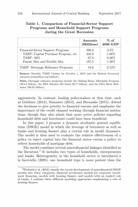
For households, the U.S. government pledged only $37.5 billionto refinance home mortgages of those who were in a negative equityposition due to the sharp decline in house prices. This amount wastiny compared with the funds to support the financial sector. Ontop of that, less than one-half of the pledged funds, $18 billion, havebeen actually spent. Table 1 reports this stark contrast between thetwo types of post-crisis government interventions.
Many prominent economists, such as Geanakoplos (2010),Stiglitz (2010), Shiller (2012), and Mian and Sufi (2014), criticizethe approach biased toward the rescue of financial institutions andargue that more grants for household debt reduction would have pro-vided a significant boost to the economy lacking aggregate demand.Mian and Sufi (2014) claim that the biggest policy mistake of theGreat Recession was not to push for mortgage write-downs more
5The Emergency Economic Stabilization Act authorized the U.S. Treasuryto purchase “troubled assets” worth $700 billion in October 2008. Part of theTARP funds, $245 billion, were used to increase banks’ capital. Most banksreceived funds through the Capital Purchase Program, while Bank of America andCitigroup additionally received $20 billion each under the Targeted InvestmentProgram.
6The Treasury purchased AIG preferred stock twice: the first purchase was$40 billion in November 2008 and the second was $27.8 billion in January 2009.
216 International Journal of Central Banking September 2017
Table 1. Comparison of Financial-Sector SupportPrograms and Household Support Programs
during the Great Recession
Amounts % of($Billions) 2008 GDP
Financial-Sector Support Programs 500.2 3.4%TARP: Capital Purchase Program, etc. 244.9 1.66%TARP: AIG 67.8 0.46%Fannie Mae and Freddie Mac 187.5 1.28%
TARP: Mortgage Refinance Programs 18.0 0.12%
Source: Monthly TARP Update for October 1, 2015 and the Bailout Scorecard(projects.propublica.org/bailout).
Note: Mortgage refinance programs include the Making Home Affordable Program($12.2 billion), the HFA Hardest Hit Fund ($5.7 billion), and the FHA Short Refi-nance ($0.02 billion).
aggressively. In contrast, leading policymakers at that time, suchas Geithner (2014), Summers (2014), and Bernanke (2015), defendthe decisions to give priority to financial rescues and emphasize theimportance of the credit channel working through financial institu-tions, though they also admit that more active policies regardinghousehold debt and foreclosure could have been beneficial.
In this paper, I propose a dynamic stochastic general equilib-rium (DSGE) model in which the leverage of borrowers as well asbanks and housing finance play a crucial role in model dynamics.The model is then used to evaluate the relative effectiveness of apolicy to inject capital into the financial sector versus a policy torelieve households of mortgage debt.
The model combines several macrofinancial linkages identified inthe literature.7 It includes two types of households, entrepreneursand banks. Heterogeneity in the household sector is introduced ala Iacoviello (2005): one household type is more patient than the
7Wieland et al. (2016) classify the recent development of macrofinancial DSGEmodels into three categories: financial accelerator models for corporate invest-ment financing, models with housing finance, and models with an explicit roleof banks. I combine three different modeling approaches emphasizing a role ofhousing finance.

Vol. 13 No. 3 Capital Injection to Banks vs. Debt Relief to HHs 217
other. In equilibrium, patient households become savers and ulti-mately supply funds to the economy, while impatient householdsare borrowers. The impatient households and entrepreneurs borrowfunds from banks using real estate as collateral. My model deviatesfrom the standard housing finance models in which borrowing isrestricted to a certain fraction of collateral and there is no default. Iintroduce an agency problem between borrowers and banks by usingthe costly state verification (CSV) setup of Gale and Hellwig (1985).It implies that the model allows for default in equilibrium. UnlikeBernanke, Gertler, and Gilchrist (1999), I assume that the contrac-tual interest rates are predetermined rather than state contingent.Accordingly, banks make zero expected profits in the perfectly com-petitive retail loan market, but ex post profits mostly differ fromzero. In my model, banks face a leverage constraint making thedeviation of the leverage ratio from its target costly as in Geraliet al. (2010). With this leverage constraint, realized profits or lossescan affect credit supply. The financial frictions described above areembedded into an otherwise standard New Keynesian model withprice and nominal wages rigidities.
The relationship between interest rate spreads and the relatedleverage ratios can describe key macrofinancial linkages in the model.The risky debt contracts imply that the interest rate spread ofeach contractual loan rate over the wholesale loan rate, the ratethat serves as a benchmark in the retail lending business, positivelydepends on the leverage of each borrower. Similarly, the bank’s opti-mal decision shows that the interest rate spread of the wholesale loanrate over the deposit rate positively varies with the bank’s leverageposition. For example, when the leverage of impatient householdsdecreases for some reason, the lending rate spread of home mort-gages also narrows, reflecting a decline in default. Faced with lowerfunding costs, borrower households increase consumption. Mean-while, realized bank profits due to lower default costs help expandingcredit availability. All other things being equal, it further boosts theexpenditure of credit-constrained agents, impatient households, andentrepreneurs.
Having in mind that most of the funds to support the financialsector presented in table 1 were injected or committed in one or twoquarters after the announcement, I model each policy as a one-timetransfer from credit-unconstrained (patient) households to either
218 International Journal of Central Banking September 2017
banks or credit-constrained (impatient) households in policy exper-iments. The capital injection to banks increases the current period’snet worth of banks, while the debt relief to credit-constrained house-holds reduces the outstanding home mortgages. The main findingsfrom the policy experiments are the following
When the economy is near the steady state and policy rates areset according to a Taylor-type rule, the capital injection to banksis more effective in stimulating the economy over the long run.Even though the debt relief to credit-constrained households has astronger effect on output for the first year, the capital injection policydominates from the second year onward. The capital injections leadinvestment to increase, which in turn expands production capacityand results in lower inflation. On the contrary, the debt relief is infla-tionary and calls for an increase of the policy rate, which reducesinvestment and the consumption of credit-unconstrained households.In the middle of the housing debt crisis, however, a debt relief policycan be more effective. This is because in such a highly leveraged sit-uation, this policy can reduce the default risk posed by high leverageto a greater extent, thereby resulting in a lower lending rate spreadof home mortgages, smaller wasteful foreclosure costs, and a greatershort-run stimulus for consumption.
When in addition the zero lower bound (ZLB) constraint is con-sidered, both policies give rise to larger effects on output and helpthe economy to escape from a liquidity trap earlier than it wouldwithout any policy.8 More interestingly, the effects of the debt reliefpolicy are magnified. The policy-induced inflation under the ZLBconstraint leads to a lower real interest rate. The decrease in thereal rate boosts investment as well as consumption, or at least signif-icantly weakens crowding-out effects. Therefore, in this environmentthe debt relief can be much more effective in stimulating the economyboth in the short run and in the long run. Moreover, the effects of thedebt relief policy on output become increasingly larger as the numberof periods that the policy rate is constrained at zero increases.
My model builds on a large literature incorporating financialfrictions into a DSGE model, including the prominent groundworksuch as Carlstrom and Fuerst (1997), Kiyotaki and Moore (1997),
8A liquidity trap is usually defined as the situation in which policy rates cannotfall below zero given that hoarding cash offers an alternative to holding deposit.

Vol. 13 No. 3 Capital Injection to Banks vs. Debt Relief to HHs 219
and Bernanke, Gertler, and Gilchrist (1999). This earlier work andmost of the subsequent research focus on an agency problem betweenfinancial intermediaries and their borrowers. These kinds of finan-cial frictions imply that the balance sheets of borrowers becomea key factor to explain macrofinancial linkages by affecting creditdemand. Recently, in particular after the recent global financialcrisis, there has been a growing literature focusing on the agencyproblem between financial intermediaries and their creditors (e.g.,Gertler and Karadi 2011, Christiano and Ikeda 2013, and Kiley andSim 2014). In those approaches, the balance sheets of financial insti-tutions play an important role in real economy by shifting creditsupply. This paper contributes to another growing literature thatconsiders financial frictions in both credit demand and credit sup-ply at the same time and puts an emphasis on their interactions. Itincludes Gerali et al. (2010), Benes and Kumhof (2011), Clerc et al.(2015), and Iacoviello (2015).
This paper is also related to recent work analyzing the macro-economic effects of housing prices during the Great Recession. Liu,Wang, and Zha (2013) and Guerrieri and Iacoviello (2015a) find thata collapse in housing prices can explain most of the sharp declinein aggregate demand, while Justiniano, Primiceri, and Tambalotti(2015) argue that such fall in housing prices was not enough to putthe economy into a deep recession. As for the modeling of homemortgage default, I follow recent approaches that model default as aput option and impose no direct foreclosure costs on borrower house-holds (for instance, Forlati and Lambertini 2011, Jeske, Krueger, andMitman 2013, Landvoigt 2014, and Quint and Rabanal 2014).
Regarding policy experiments, a number of papers analyze themacroeconomic consequences of injecting more capital into banksusing a DSGE model with a leverage constraint for banks (seeHirakata, Sudo, and Ueda 2013, Kollmann et al. 2013, Kiley andSim 2014, van der Kwaak and van Wijnbergen 2014, Guerrieri etal. 2015, etc.) Most of them find that the capital injection policyhas positive effects on output since it increases credit supply tothe productive but credit-constrained sector. In contrast, only a fewinvestigate the macroeconomic effects of reducing household debt.Guerrieri and Iacoviello (2015a) analyze the effects of a lump-sumtransfer from credit-unconstrained households to credit-constrainedhouseholds using a DSGE model with the presence of an occasionally

220 International Journal of Central Banking September 2017
binding constraint, and find that such a transfer can have sizableeffects on output when the borrowing constraint binds. Mian andSufi (2014) estimate the macroeconomic effects of the introductionof shared-responsibility mortgages, which in essence feature an auto-matic principal reduction when housing prices decline below thepurchasing level.9 They put into perspective several empirical stud-ies such as Mian, Rao, and Sufi (2013), Nakamura and Steinsson(2014), and Mian, Sufi, and Trebbi (2015). They argue that theoutput effects of new mortgage contracts would be large enough tosubstantially reduce the severity of the recession. Dogra (2014) usesa simple model in which the economy hits the ZLB by householddeleveraging and analyzes the effects of debt relief modeled as atargeted transfer. He finds that debt relief stimulates the economy,but the anticipation of debt relief leads to overborrowing. He shows,nevertheless, that optimal policy is still involved in the use of debtrelief up to a certain level.
My contributions to the literature are, first, to design a rigorouspolicy experiment to reduce households’ debt in a structural macromodel and to compare the relative effectiveness of this policy andthe policy to increase banking capital. Second, as an additional nov-elty, this paper evaluates those policies considering the zero lowerbound, following a new literature to assess fiscal stimulus with theassumption of monetary accommodation (see Cogan et al. 2010,Coenen et al. 2012, and Eggertsson and Krugman 2012). Lastly butnot least, the model proposed in this paper applies the financialaccelerator mechanism to business loan contracts collateralized bycommercial real estate. With this modeling device the model impliesthat a decline in housing prices leads to a decrease in non-residentialinvestment as well as a rise in default on business loans, which is con-sistent with the empirical evidence. If a standard modeling setup forhousing as in Iacoviello and Neri (2010) is simply combined with astandard risky debt contract for corporate financing as in Bernanke,Gertler, and Gilchrist (1999), then the model implies that a fall inhousing prices accompanies a business investment boom.
9Shared-responsibility mortgages have two important features that are dis-tinct from the existing ones: the bank offers the protection to borrowers whenhouse prices decline below the purchasing price, while the bank obtains 5 percentcapital gains when house prices increase over the purchasing level.

Vol. 13 No. 3 Capital Injection to Banks vs. Debt Relief to HHs 221
The remainder of this paper is organized as follows. Section 2describes the model economy and defines the competitive equilib-rium. Section 3 explains the calibration strategy and its results.Section 4 analyzes the results from a series of simulations, andsection 5 concludes.
2. The Model Economy
Time is discrete and quarterly. The economy is populated by a con-tinuum of two types of infinitely lived households. Each householdhas unit mass. They differ in their discount factors. One type ismore patient than the other. A household obtains utility from con-sumption and housing services and disutility from labor. Within thehousehold, perfect risk sharing is provided to its members. The nom-inal wages are set by each type’s monopolistic labor union. Each ofthe patient households has a large number of entrepreneurs, andowns banks, intermediate goods producing firms, retail firms, andcapital goods producing firms.
Banks channel funds from patient households (and the banks’own net worth) to impatient households and entrepreneurs. Eachbank consists of a wholesale branch and two retail branches. Oneretail branch deals with home mortgages, while the other handlesbusiness loans. The wholesale branch issues wholesale loans to thetwo retail branches subject to a leverage constraint such that it paysa pecuniary cost for the deviation of the bank net-worth-to-assetratio from its target. When it comes to the retail lending business,an agency problem arises because the return to the underlying assetsposted as collateral is subject to idiosyncratic risk and the realiza-tion of an individual shock can only be observed by the bank afterpaying some cost. Consequently, each retail branch makes an exante risky debt contract with its borrowers. Bank profits or lossesare accumulated into its net worth after a fraction of the net worthis transferred to patient households.
Entrepreneurs combine loans with their net worth to purchaseraw non-residential capital and new residential capital. Then theyprovide the composite capital services to intermediate goods pro-ducing firms that use them with two types of labor to produce inter-mediate goods. Retail firms operate under monopolistic competitionand are subject to implicit costs to adjust nominal prices following
222 International Journal of Central Banking September 2017
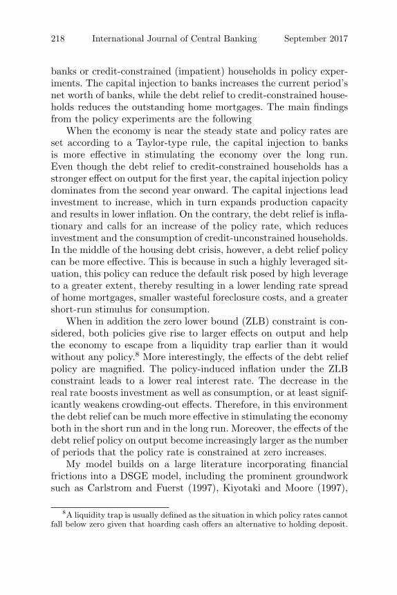
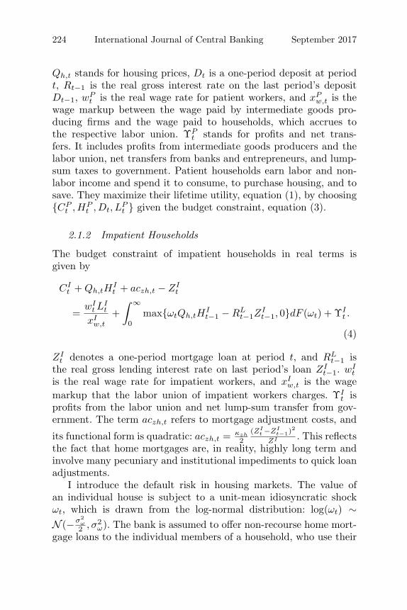
Figure 1. Model Structure
Calvo-style contracts. The constant-elasticity-of-substitution (CES)aggregates of these goods are converted into homogenous final goods.Capital goods producing firms purchase previously installed depre-ciated capital from entrepreneurs and investment goods from finalgood producing firms, and produce new installed capital subject toinvestment adjustment costs.
Aggregate housing supply is assumed to be fixed.10 The centralbank sets the nominal risk-free interest rate according to a Taylor-type rule. The government can collect lump-sum taxes from patienthouseholds and give them out to other agents. The structure of themodel is depicted in figure 1. In the following, I describe the decisionproblems of each agent and define the competitive equilibrium of themodel economy.
10Basically, I exclude residential investment and its spillover effects on thebroad economy from the analysis.

Vol. 13 No. 3 Capital Injection to Banks vs. Debt Relief to HHs 223
2.1 Households
The household sector is composed of two types of households. Thediscount factor of patient households is higher than that of impa-tient households (βP > βI). Each household (s ∈ {P, I}) maximizesthe expected discounted sum of per-period utility:
V sH = E0
∞∑
t=0
(βs)t
{Γs log(Cs
t − εCst−1) + χs
t log Hst − ψl
(Lst )
1+ϕ
1 + ϕ
}.
(1)
Cst denotes consumption, Hs
t refers to the housing stock owned byeach household, and Ls
t denotes labor supplied. I assume habit for-mation in consumption. As in Iacoviello (2005), utility from housingservices is proportionate to the housing stock, and utility is separablein consumption and housing. Γs is used for normalization such thatthe marginal utilities of consumption at the non-stochastic steadystate are the inverse of consumption: Γs = 1−ε
1−βsε . I allow for thepossibility that each type of household values one unit of housingservices differently. Housing preferences are subject to shocks. Adecrease in χs
t moves preferences away from housing and towardsconsumption and leisure, so that housing demand decreases and, inthe end, housing prices fall.11 The shock process for each type isgiven by
log(χst ) = (1 − ρχ) log(χs) + ρχ log(χs
t−1) + εχ,t s ∈ {P, I}. (2)
In equilibrium, patient households are savers and impatient house-holds are borrowers. For simplicity, I describe each type’s decisionproblem, taking these equilibrium outcomes into account.
2.1.1 Patient Households
The budget constraint of patient households in real terms is
CPt + Qh,t(HP
t − HPt−1) + Dt =
wPt LP
t
xPw,t
+ Rt−1Dt−1 + ΥPt . (3)
11For this reason, the shock on housing preferences is also called a housingdemand shock.
224 International Journal of Central Banking September 2017
Qh,t stands for housing prices, Dt is a one-period deposit at periodt, Rt−1 is the real gross interest rate on the last period’s depositDt−1, wP
t is the real wage rate for patient workers, and xPw,t is the
wage markup between the wage paid by intermediate goods pro-ducing firms and the wage paid to households, which accrues tothe respective labor union. ΥP
t stands for profits and net trans-fers. It includes profits from intermediate goods producers and thelabor union, net transfers from banks and entrepreneurs, and lump-sum taxes to government. Patient households earn labor and non-labor income and spend it to consume, to purchase housing, and tosave. They maximize their lifetime utility, equation (1), by choosing{CP
t , HPt , Dt, L
Pt } given the budget constraint, equation (3).
2.1.2 Impatient Households
The budget constraint of impatient households in real terms isgiven by
CIt + Qh,tH
It + aczh,t − ZI
t
=wI
t LIt
xIw,t
+∫ ∞
0max{ωtQh,tH
It−1 − RL
t−1ZIt−1, 0}dF (ωt) + ΥI
t .
(4)
ZIt denotes a one-period mortgage loan at period t, and RL
t−1 isthe real gross lending interest rate on last period’s loan ZI
t−1. wIt
is the real wage rate for impatient workers, and xIw,t is the wage
markup that the labor union of impatient workers charges. ΥIt is
profits from the labor union and net lump-sum transfer from gov-ernment. The term aczh,t refers to mortgage adjustment costs, and
its functional form is quadratic: aczh,t = κzh
2(ZI
t −ZIt−1)
2
ZI . This reflectsthe fact that home mortgages are, in reality, highly long term andinvolve many pecuniary and institutional impediments to quick loanadjustments.
I introduce the default risk in housing markets. The value ofan individual house is subject to a unit-mean idiosyncratic shockωt, which is drawn from the log-normal distribution: log(ωt) ∼N (−σ2
ω
2 , σ2ω). The bank is assumed to offer non-recourse home mort-
gage loans to the individual members of a household, who use their

Vol. 13 No. 3 Capital Injection to Banks vs. Debt Relief to HHs 225
individual housing as collateral. I further assume that there is nodirect cost for households who default. Default, namely, is modeledas a put option. Each member indexed by j decides whether or notto default based on the realization of an individual shock, with theaim to maximize the individual net worth.
max{ωtQh,tHIt−1(j) − RL
t−1ZIt−1(j)︸ ︷︷ ︸
No default
, 0︸︷︷︸Default
}
The optimal decision rule puts the default threshold ωt at
ωt =RL
t−1ZIt−1(j)
Qh,tHIt−1(j)
=RL
t−1ZIt−1
Qh,tHIt−1
=mt−1
Δh,t. (5)
The individual members will default on mortgages if mortgage repay-ment obligations are greater than their housing values. As each mem-ber’s holdings of mortgages are proportional to that of housing, theindex j can be dropped. ωt can be expressed in terms of the loan-to-value ratio of the previous period, mt−1 = RL
t−1ZIt−1
Qh,t−1HIt−1
, and the ex
post average return on housing, Δh,t = Qh,t
Qh,t−1. The default threshold
ωt increases in the household’s leverage and decreases in the real-ized return on housing. Using the default threshold ωt, the budgetconstraint can be rewritten as
CIt + Qh,tH
It + aczh,t − ZI
t ≤ wIt LI
t
xIw,t
+ [1 − Γ(ωt)]Qh,tHIt−1 + ΥI
t ,
(6)
where Γ(ωt) is the share of the housing value going to the bank.12
Due to an agency problem, the bank retail branch of home mort-gages incurs a cost proportional to the value of foreclosed houseswhen it forecloses on mortgages. Accordingly, such a risky debt con-tract must satisfy the following ex ante participation constraint ofthe bank:
Et{(Γ(ωt+1) − μBG(ωt+1))Qh,t+1HIt } ≥ Rr
t ZIt . (7)
12F (ωt) =∫ ωt
0 dF (ωjt ; σω) is the foreclosure rate; G(ωt) =
∫ ωt
0 ωjt dF (ωj
t ; σω)denotes a fraction of the foreclosed houses of impatient households; Γ(ωt) areexpressed by [1 − F (ωt)]ωt + G(ωt).
226 International Journal of Central Banking September 2017
μB is a foreclosure cost parameter, and Rrt is the wholesale real lend-
ing interest rate that serves as a benchmark rate in retail lending.13
This constraint states that the expected gain of the bank’s contribu-tion to housing investment net of foreclosure cost is at least as highas its funding cost. Finally, impatient households maximize theirlifetime utility, equation (1), with respect to {CI
t , HIt , ZI
t , mt, LIt }
subject to the budget constraint, equation (6), and the bank’s par-ticipation constraint, equation (7).
It is worth noting that the participation constraint of the bankholds with equality. It means that the retail branch would makeunexpected profits or losses in equilibrium depending on the realiza-tion of certain aggregate shocks. Such unexpected profits, εhb,t, are afunction of endogenous variables, including the default threshold ωt.
εhb,t = (Γ(ωt) − μBG(ωt))Qh,tHIt−1 − Rr
t−1ZIt−1 (8)
In addition, the binding participation constraint of the bank impliesthat the interest rate spread of the contractual lending rate onmortgages RL
t over the wholesale lending rate Rrt is a function of
the default threshold ωt+1 in expectation.14 As the right-hand sideof equation (9) is an increasing function of ωt+1, the interest ratespread rises when the leverage of borrowers increases.15
RLt
Rrt
= Et
{ωt+1
Γ(ωt+1) − μBG(ωt+1)
}(9)
2.1.3 Nominal Wage Decisions
Nominal wage stickiness is introduced in a way analogous to nom-inal price stickiness as in Smets and Wouters (2007) and Iacovielloand Neri (2010). Each type of household supplies its homogenouslabor services to the labor union that serves the interest of each
13Alternately, the wholesale lending rate can be thought of as the rate whichbanks would charge to notional zero-risk borrowers (see Benes and Kumhof 2011).
14Plugging equation (5) into equation (7) holding with the equality, we obtainequation (9).
15Suppose that Ω(x) = xΓ(x)−μBG(x) . Then Ω′(x) = (1−μB)G(x)+x2f(x)
(Γ(x)−μBG(x)6)2 > 0 forall x > 0. Here, f(x) is a density function of the log-normal distribution.
Vol. 13 No. 3 Capital Injection to Banks vs. Debt Relief to HHs 227
type.16 Each union differentiates labor services, sets nominal wagessubject to Calvo-style adjustment frictions, and offers labor servicesto the respective labor packer. Each representative and competi-tive labor packer aggregates the differentiated labor services intothe homogeneous labor services, which are hired by intermediategoods producing firms. The optimal wage rates set by each laborunion together with the evolution formula for real wages imply thefollowing wage Phillips curves:
log(
ΠwP ,t
Π
)= βP Et log
(ΠwP ,t+1
Π
)− κP
w log
(xP
w,t
xPw
)(10)
log(
ΠwI ,t
Π
)= βIEt log
(ΠwI ,t+1
Π
)− κI
w log
(xI
w,t
xIw
), (11)
where ΠwP ,t = wPt Πt/wP
t−1 and ΠwI ,t = wIt Πt/wI
t−1 refer towage inflation for patient and impatient households, respectively.κP
w = (1−θwP )(1−βP θwP )/θwP and κIw = (1−θwI )(1−βIθwI )/θwI
define the slope of each wage equation. Π denotes the non-stochasticsteady states of inflation. xP
w and xIw are the wage markup of the
patient and impatient households, each.
2.2 Entrepreneurs
Entrepreneurs are modeled in the same way as in Bernanke, Gertler,and Gilchrist (1999) and Christiano, Motto, and Rostagno (2014)with two exceptions. First, the contractual interest rates are pre-determined rather than being state contingent. Second, entrepre-neurs deal with two types of capital—residential capital and non-residential capital.17 Each patient household has a large number ofentrepreneurs indexed by j, whose state is summarized by their networth, NE
t (j). Each entrepreneur j obtains a loan ZEt (j) from the
bank’s retail branch for business loans and combines it with his net
16The essence of wage staggering is to give workers bargaining power to decidewages for a certain period. Equivalently, we can assume that each monopolisticcompetitive household supplies differentiated labor services to the labor packerand sets nominal wages in a Calvo-style staggering contract.
17In this paper, residential capital is used interchangeably with commercial realestate.

228 International Journal of Central Banking September 2017
worth NEt (j) to purchase raw non-residential capital Kt(j) at a price
of Qk,t and new residential capital HEt (j) − HE
t−1(j) at a price ofQh,t. The balance sheet of each entrepreneur at the end of time t isgiven by
Qk,tKt(j) + Qh,tHEt (j) = ZE
t (j) + NEt (j). (12)
At period t + 1, entrepreneurs provide composite capital ser-vices, Kt = HE
t (j)νkKt(j)1−νk , to intermediate goods produc-
ers. The return to the composite capital, ωe,t+1(Rkt+1Qk,tKt(j) +
Rht+1Qh,tH
Et (j)), is assumed to be sensitive to both idiosyncratic
and aggregate shocks. An idiosyncratic shock ωe,t is modeled tofollow a log-normal distribution: log ωe,t ∼ N(−σ2
eω
2 , σ2eω), with
Etωe,t = 1. The rates of return to non-residential and residentialcapital are given by
Rkt+1 =
rk,t+1 + (1 − δk)Qk,t+1
Qk,t, (13)
Rht+1 =
rh,t+1 + Qh,t+1
Qh,t. (14)
rk,t+1 and rh,t+1 are competitive market rental rates for non-residential and residential capital, respectively. Non-residential cap-ital depreciates at a quarterly rate of δk. As can be seen in equations(13) and (14), an aggregate shock can affect the return to compositecapital via either the rental rates or capital prices or both. Note thatRk
t+1 and Rkt+1 are equal across entrepreneurs indexed by j. Similarly
to the default threshold of impatient households, equation (5), thedecision rule for the entrepreneurs’ default threshold is expressed by
ωe,t+1 =RE
t ZEt (j)
Rkt+1Qk,tKt(j) + Rh
t+1Qh,tHEt (j)
. (15)
REt denotes the real gross lending rate on the business loan ZE
t .It is worth noting that ωe,t+1 is independent of the entrepreneur’snet worth and thus her net worth only matters for the size of acertain project. In what follows, I drop the index, j, for notationalconveniences. If the realized idiosyncratic shock is below the defaultthreshold, ωe,t+1 < ωe,t+1, then entrepreneurs default and hand over
Vol. 13 No. 3 Capital Injection to Banks vs. Debt Relief to HHs 229
all remaining resources to the bank. Meanwhile, the business loanbranch has to pay an auditing cost μE proportional to the assetsof the bankrupt entrepreneurs due to asymmetric information. Ifωe,t+1 ≥ ωe,t+1, entrepreneurs repay debt RE
t ZEt while keeping the
surplus return to investment. Therefore, the contractual terms ofsuch a risky debt must satisfy the following ex ante participationconstraint of the bank:
Et
{(1 − F (ωe,t+1))RE
t ZEt + (1 − μE)
∫ ωe,t+1
0ωe,t(Rk
t+1Qk,tKt
+ Rht+1Qh,tH
Et )f(ωe,t)dωe,t
}≥ Rr
t ZEt . (16)
Here, F (ωe,t+1) is the default rate for business loans.18 Finally, eachentrepreneur maximizes his share of the expected gross return ofcapital investment in period t + 1, Et{(1 − Γ(ωe,t+1)(Rk
t+1Qk,tKt +Rh
t+1Qh,tHEt )}, subject to equations (12) and (16). I define two vari-
ables for entrepreneurial leverage: φkt = Qk,tKt
NEt
, φht = Qh,tH
Et
NEt
. Bothleverage ratios increase when the entrepreneur’s net worth decreases.Each leverage variable also increases when the respective asset pricesdecline. After some algebra, the entrepreneur’s maximization prob-lem can be reformulated as
maxφk
t ,φht ,ωe,t+1
Et{(1 − Γ(ωe,t+1))(Rkt+1φ
kt + Rh
t+1φht )}NE
t (17)
subject to
Et{[Γ(ωe,t+1) −μEG(ωe,t+1)](Rkt+1φ
kt + Rh
t+1φht )} = Rr
t (φkt + φh
t − 1).
The default threshold can be rewritten in terms of leverage vari-ables: ωe,t+1 = RE
t (φkt +φh
t −1)Rk
t+1φkt +Rh
t+1φht. As the first-order conditions imply
that EtRk
t+1Rr
t= Et
Rht+1Rr
t, we find that the expectation of ωe,t+1
18In addition, Γ(ωe,t+1) denotes a fraction of gross return of capital investmentgoing to the banks, and G(ωe,t+1) refers to a fraction of the defaulted value ofcomposite capital. The mathematical expressions are the same as in footnote 12.

230 International Journal of Central Banking September 2017
increases with total leverage of entrepreneurs, φkt + φh
t .19 The retailbranch for business loans would make unexpected profits in equilib-rium according to the realization of a certain aggregate shock. Suchprofit surprises, εeb,t, are expressed by
εeb,t = (Γ(ωe,t) − μEG(ωe,t))(Rkt Qk,t−1Kt−1 + Rh
t Qh,t−1HEt−1)
− Rrt−1Z
Et−1. (18)
Also, reformulations of the participation constraint of banks usingthe default threshold ωe,t+1 show that the lending rate spread ofbusiness loans is a function of the default threshold ωe,t+1 in expecta-tion. As the right-hand side of equation (19) is an increasing functionof ωe,t+1, the lending rate spread increases when the entrepreneurialleverage goes up.20
REt
Rrt
= Et
{ωe,t+1
(Γ(ωe,t+1) − μEG(ωe,t+1))
}(19)
At the end of the period t + 1, a fraction (1 − γ) of each entre-preneur’s net worth is transferred to his own household and eachentrepreneur receives a lump-sum transfer W e from the household.Since the ex post net worth of an individual entrepreneur is linear, wecan simply integrate individual entrepreneurs’ net worth and derivethe evolution of total net worth of entrepreneurs as follows:
NEt = γ[(1 − Γ(ωe,t))(Rk
t φkt−1 + Rh
t φht−1)}NE
t−1] + W e. (20)
19The first-order conditions are given by
Et
{(1 − Γ(ωe,t+1))
Rkt+1
Rrt
+Γ′(ωe,t+1)
Γ′(ωe,t+1) − μEG′(ωe,t+1)
×[(Γ(ωe,t+1) − μEG(ωe,t+1))
Rkt+1
Rrt
− 1]}
= 0,
Et
{(1 − Γ(ωe,t+1))
Rht+1
Rrt
+Γ′(ωe,t+1)
Γ′(ωe,t+1) − μEG′(ωe,t+1)
×[(Γ(ωe,t+1) − μEG(ωe,t+1))
Rht+1
Rrt
− 1]}
= 0.
With EtRk
t+1Rr
t= Et
Rht+1Rr
tit holds that E{ωe,t+1} = RE
t (φkt +φh
t −1)Rk
t+1φkt +Rh
t+1φht
= 1 − 1φk
t +φht.
20Refer to footnote 15.
Vol. 13 No. 3 Capital Injection to Banks vs. Debt Relief to HHs 231
2.3 Banks
Following Gerali et al. (2010), I assume that there is a unit mass ofbanks and each bank consists of two retail branches and one whole-sale branch. The first retail branch is responsible for providing homemortgages ZI
t to impatient households. The second retail branchgives out business loans ZE
t to entrepreneurs. I also assume thatboth retail branches operate in perfect competition. They obtainwholesale loans at the wholesale rate Rr
t and sell them to final bor-rowers on the condition that the ex ante participation constraintof the bank holds. Therefore, each retail branch sets the contrac-tual lending rate according to equations (9) and (19), respectively.Then the retail branches pass over resulting profits or losses to thewholesale branch.
The wholesale branch has a net worth Nt, which is accumulatedout of retained profits, and collects deposits Dt from patient house-holds at the deposit rate Rt. With these funds the wholesale branchissues wholesale loans Wt at the wholesale rate Rr
t while paying alinear operating cost κwWt and a quadratic penalty cost when thebank net-worth-to-asset ratio Nt/Wt deviates from its target. Theproblem of the wholesale branch is to choose loans and depositsto maximize the discounted sum of expected profits subject to thebalance sheet constraint:
max{Wt,Dt}
E0
∞∑
t=0
(βP )t+1ΛP0,t+1Πwb,t+1, (21)
where
Πwb,t+1 = Rrt Wt + Πhb,t+1 + Πeb,t+1 − RtDt
− Nt − κwWt − φn
2
(Nt
Wt− νb
)2
Nt
subject to
Wt = ZIt + ZE
t = Nt + Dt.
Here, Πhb,t+1 denotes total profits of the home mortgage branch;Πeb,t+1 refers to those of the business loan branch. Due to the bind-ing participation constraints of the bank, profits or losses resulting

232 International Journal of Central Banking September 2017
from an ex ante risky debt contract, εhb,t and εeb,t, are an unex-pected surprise by construction.21 To improve empirical validity, Iassume that εhb,t and εeb,t have persistent effects on the bank’s networth with a decaying factor (ρh and ρe, respectively), albeit adhoc.22 Then Πhb,t and Πeb,t are expressed by
Πhb,t = εhb,t + ρhεhb,t−1 + ρ2hεhb,t−2 + ρ3
hεhb,t−3 + · · · ,
Πeb,t = εeb,t + ρeεeb,t−1 + ρ2eεeb,t−2 + ρ3
eεeb,t−3 + · · · .
The above equations can be reformulated in autoregressive form:
Πhb,t = εhb,t + ρhΠhb,t−1, (22)
Πeb,t = εeb,t + ρeΠeb,t−1. (23)
The first-order condition of the wholesale branch’s problem isgiven by
Rrt − Rt = κw − φn
(Nt
Wt− νb
) (Nt
Wt
)2
. (24)
Since the right-hand side of equation (24) is decreasing in the banknet-worth-to-asset ratio around the steady state, the interest ratespread between the wholesale loan rate and the deposit rate increases(up to the first-order approximation) when the bank’s leverage goesup. All bank profits are reinvested in banking activity and a frac-tion (δb) of the pre-profit bank net worth is transferred to its ownhousehold. Aggregate bank capital evolves according to
Nt = (1 − δb)Nt−1 + Πwb,t. (25)
21Et[εhb,t+1] = 0, Et[εeb,t+1] = 0.22I take an approach similar to Guerrieri et al. (2015) that employs an autore-
gressive process of order 1 for bank losses in their simulations based on an empir-ically relevant scenario used in the stress tests for the U.S. banking sector. Theintroduction of the ad hoc adjustment implies a stronger role of the bank’s networth in model dynamics than otherwise. It does not, however, change simulationresults qualitatively.
Vol. 13 No. 3 Capital Injection to Banks vs. Debt Relief to HHs 233
2.4 Production Sector and Nominal Rigidities
In order to introduce price rigidities, I differentiate between com-petitive intermediate goods producing firms and retail firms. Inter-mediate goods producing firms hire composite capital services fromentrepreneurs and two types of labor from households and solve thefollowing maximization problem given their production technology.
max{LP
t ,LIt ,Kt−1,HE
t−1}
{Yt
xp,t− wP
t LPt − wI
t LIt − rk,tKt−1 − rh,tH
Et−1
},
(26)
where
Yt = [HEt−1
νkKt−1
1−νk ]α[LPt
νlLI
t
(1−νl)](1−α).
xp,t is the price markup of final goods over intermediate goods.Retail firms operate in a regime of monopolistic competition andface Calvo-type nominal price frictions. Retailers buy intermedi-ate goods Yt at the price Pw
t in a competitive market, differenti-ate the goods, and sell them at price Pt, which includes a markupxp,t = Pt/Pw
t over the marginal cost Pwt . The CES aggregates of
these goods are converted into homogenous final goods, which arepurchased by households and capital good producing firms. In everyperiod, each retail firm sets optimal prices with probability 1 − θπ
or indexes prices to the steady-state inflation Π with probability θπ,regardless of the history of its price adjustments. These assumptionsdeliver the following price Phillips curve:
log(
Πt
Π
)= βP Et log
(Πt+1
Π
)− κπ log
(xp,t
xp
), (27)
where κπ = (1−θπ)(1−βP θπ)θπ
determines the sensitivity of inflation tochanges in the price markup xp,t relative to its steady-state value xp.
Capital goods producing firms purchase previously installeddepreciated capital from entrepreneurs and investment goods It fromfinal goods producing firms, and produce new installed capital sub-ject to investment adjustment costs. The capital goods producersolves
maxIτ
Et
∞∑
τ=t
Λt,τ
{Qk,τIτ −
[1 + sk
(Iτ
Iτ−1
)]Iτ
}, (28)
234 International Journal of Central Banking September 2017
where sk(x) = κk
2 (x − 1)2. The aggregate non-residential capitalevolves according to
Kt+1 = (1 − δk)Kt + It. (29)
2.5 Central Bank and Government
The central bank sets the risk-free nominal interest rate based onan interest rate feedback rule that allows for interest rate smoothingand reacts to annual inflation and output.
Rnt = max
{1, (Rn
t−1)γR
(ΠA
t
ΠA
)(1−γR)γπ (Yt
Y
)(1−γR)γy
(Rn)1−γR
},
(30)
where ΠAt is year-on-year inflation, which is expressed in quarterly
terms as ΠAt = (Pt/Pt−4)1/4. The link between nominal and real
interest rates is given by the Fisher equation: Rnt = Rt · EtΠt+1.
Government uses fiscal policy only for redistributive purposes:TrP
t + TrIt = 0. In the baseline model I ignore the redistributive
role of the government.
2.6 Competitive Equilibrium
The model is closed by market clearing conditions. As aggregatehousing supply is normalized to one, the housing market clears asbelow:
HPt + HI
t + HEt = 1. (31)
By Walras’s law, the good’s market clears:
Yt = CPt + CI
t +[1 + sk
(It
It−1
)]It + Adjt,
where Adjt = μBG(ωt; )Qh,tHIt−1 + μEG(ωe,t)(Rk
t Qk,t−1Kt−1 +Rh
t Qh,t−1HEt−1) + κwWt + φn
2 ( Nt
Wt− νb)2Nt + aczh,t.
The competitive equilibrium consists of a set of prices {Rt,RLt ,RE
t ,Rr
t , Rkt , Rh
t , Qh,t, Qk,t, rh,t, rk,t, wPt , wI
t , Πt, xp,t, xPw,t, x
Iw,t}∞
t=0 and
Vol. 13 No. 3 Capital Injection to Banks vs. Debt Relief to HHs 235
a set of real allocations {CPt , CI
t , LPt , LI
t , ΛPt , ΛI
t , HPt , HI
t , HEt , Dt,
ZIt , ZE
t , Kt, NEt , φk
t , φht , ωt, ωe,t, Nt, Πhb,t, Πeb,t, It, Yt}∞
t=0 for a givengovernment policy {Rn
t , T rPt , T rI
t }∞t=0, a realization of exogenous
variables {εχ,t}∞t=0 and initial conditions {HP
−1, HI−1, H
E−1, D−1, Z
I−1,
ZE−1, K−1, N
E−1, N−1} such that
• households of both types maximize the lifetime utility giventhe prices;
• each labor union maximizes its profits given the prices;• the entrepreneurs’ allocations solve the problem (17) given the
prices;• the banks’ allocations solve the problem (21) given the prices;• the intermediate goods firms solve the problem (26) given the
prices;• the retail firms maximize their profits given the prices;• the capital goods producing firms solve the problem (28) given
the prices;• the government budget constraint holds;• markets clear.
A set of equations describing the equilibrium of the model issummarized in the appendix of Yoo (2017).
3. Calibration
I divide the model parameters into two sets. For the first set ofparameters I choose values mostly from the relevant literature. Thesecond set of parameters is endogenously determined in the modelto ensure that the model’s steady state is consistent with the empir-ical features related to macro aggregates as well as debt and realestate owned by households and non-financial businesses for the U.S.economy during 1991–2006.
3.1 Exogenously Chosen Parameters
Exogenously chosen parameters are presented in table 2. The dis-count factor of patient households βP is set at 0.995, implying thatthe steady-state risk-free real interest rate is 2 percent. As for other

236 International Journal of Central Banking September 2017
Table 2. Exogenously Chosen Parameters
Description Parameter Value
Households, Production Sector, and Nominal Rigidities
Discount Factor, Patient Households βP 0.995Habit Formation in Consumption ε 0.65Inverse of the Frisch Elasticity ϕ 1.0Disutility Weight on Labor ψl 1.0Steady-State Price Markup xp 1.2Steady-State Wage Markup xw 1.2Probability of Keeping Prices Fixed θ 0.85Probability of Keeping Wages Fixed θw 0.9Investment Adjustment Cost κk 2.0Steady-State Inflation Π 1.005 (2%)Wage Share of Impatient Households 1 − vl 0.35
Financial Frictions
Foreclosure Cost μB 0.17Monitoring Cost μE 0.215Fraction of Entrepreneurial Net Worth 1 − γ 1–0.982
Transferred to HouseholdsTarget Capital-to-Asset Ratio vb 0.1Wholesale Funds Operating Cost κw 0.015/4Bank Capital Adjustment Cost φn 25Mortgage Adjustment Cost κzh 4.0Autocorrelation of Retail Profits, Home Mortgages ρh 0.9Autocorrelation of Retail Profits, Business Loans ρe 0.9
Others
Policy Smoothing Coefficient ρR 0.7Policy Reaction Coefficient on Inflation ρπ 2.0Policy Reaction Coefficient on Output ρy 0.5/4AR(1) Coefficient on Housing Preference Shock ρχ 0.97
conventional parameters, I choose standard values in the New Key-nesian literature. These include the consumption habit parameterε, the inverse Frisch elasticity of labor supply ϕ, the steady-stateprice markup xp, the steady-state wage markup xw, and the invest-ment adjustment cost parameter κk. The disutility weight on laborsteady ψl is normalized to 1. I set parameters governing the priceand wage rigidities, θ and θw, to 0.85 and 0.9, respectively. I choose
Vol. 13 No. 3 Capital Injection to Banks vs. Debt Relief to HHs 237
values from the mid-upper range found in the literature in order topartially compensate the absence of several real or nominal frictionssuch as variable capital utilization and partial indexation of pricesand wages to past inflation. The steady-state annual inflation is setto 2 percent. I set the steady-state wage share of impatient house-holds to 0.35, which is in the mid-range of the existing literature.23
The resulting income share of these households in aggregate incomeis 24 percent.
In choosing the parameters related to financial frictions, I relyon a number of previous studies. As in Chatterjee and Eyigungor(2015), the foreclosure cost parameter μB is set to 0.17, which meansthat banks lose 17 percent of the values of houses in case of foreclo-sure. The parameter for the monitoring cost of business loans μE istaken from Christiano, Motto, and Rostagno (2014), who estimate ittogether with other structural parameters. The parameter governingthe transfer from entrepreneurs to their respective households, 1−γ,is determined to be 1–0.982. This lies in between the 1–0.973 valueused by Bernanke, Gertler, and Gilchrist (1999) and the 1–0.985value used by Christiano, Motto, and Rostagno (2014).
Due to the binding participation constraint of the bank, themodel-implied profits and losses are unexpected and serially uncorre-lated. This implication conflicts with the data that show persistence.To improve the fit of the model, I introduce AR(1) processes (equa-tions (22) and (23)). I set the autocorrelation coefficients, ρh andρe, at 0.9, following Guerrieri et al. (2015) who conduct compar-ative exercises with regard to an exogenous shock to bank capitallosses with five structural macrofinancial models.
The parameter for the bank capital adjustment cost φn is set to25, which is roughly twice the estimated value of 11.5 in Gerali et al.(2010). It implies that the elasticity of the bank’s interest rate spreadwith respect to the bank net worth is approximately twice as big asthat in Gerali et al. (2010).24 The targeted capital-to-asset ratio νb isset to 10 percent. I consider not only the regulatory minimum capital
23The wage share of credit-constrained households used in other studies is asfollows: 0.36 in Iacoviello (2005), 0.21 in Iacoviello and Neri (2010), 0.42 in Guer-rieri and Iacoviello (2015a), etc. Using the Survey of Consumer Finances (SCF),Kaplan and Violante (2014) estimate that between 17.5 percent and 35 percentof U.S. households are liquidity constrained.
24Refer to equation (32) in footnote 37.

238 International Journal of Central Banking September 2017
requirement of 8 percent but also the additional requirement implic-itly enforced by market discipline, which seems to be consistent withU.S. data.25 The operating cost parameter at the wholesale branch ofbanks, κw, is put to 0.015/4, implying that the steady-state interestrate spread of the wholesale loan rate over the deposit rate is 1.5 per-cent in annual terms. The parameter governing mortgage adjustmentcosts is set to 4.26
As for the interest rate rule’s specification, I use 0.7 for interestrate smoothing, 2.0 for the reaction coefficient on inflation, and 0.5/4for the reaction coefficient on output. Lastly, I employ a fairly persis-tent AR(1) process for the housing preference shock as in Iacovielloand Neri (2010) and Liu, Wang, and Zha (2013).
3.2 Endogenously Determined Parameters
Endogenously determined parameters are reported in table 3together with empirical targets used for calibration. The steady-statedefault threshold for home mortgages ω and the standard deviationof an idiosyncratic shock in households’ housing σω are chosen suchthat the loan-to-value ratio of impatient households is 85 percent andthe annual foreclosure rate for home mortgages is 1.5 percent. Theformer is in line with the average loan-to-value ratios of first-timehomebuyers for the 1990s and early 2000s estimated by Duca, Muell-bauer, and Murphy (2011), and the latter is the average foreclosurerate for 1991–2006 reported by the Mortgage Bankers Association. Ina similar way, the steady-state default threshold for business loans ωe
and the standard deviation of an individual shock in entrepreneurs’capital services σωe
are calibrated to agree with both the averageof debt-to-net-worth ratio of non-financial business for 1991–2006,0.42, and the annual business default rate estimated by Christiano,Motto, and Rostagno (2014), 2.25 percent.27
25The average of the equity-to-asset ratios for the U.S. commercial banks during2004–06 is 9.9 percent.
26I conduct the sensitivity analysis in the appendix of Yoo (2017) since thereis no prior information.
27Debt of non-financial business is the sum of the credit market instruments ofboth non-financial corporate business and non-financial non-corporate business.Net worth is the sum of net worth of non-financial corporate business at marketprices and net worth of non-financial non-corporate business. All the data aretaken from tables B.102 and B.103 in Flow of Funds Accounts.

Vol. 13 No. 3 Capital Injection to Banks vs. Debt Relief to HHs 239
Table 3. Endogenously Determined Parameters andSelected Steady-State Ratios
Description Parameter Value
A. Endogenously Determined Parameters
Discount Factor, Impatient Households βI 0.9598Steady-State Housing Parameter, Patient Households χP 0.032Steady-State Housing Parameter, Impatient Households χI 0.190Capital Share in Production α 0.307Commercial Real Estate Share in Production 1 − νk 0.050Depreciation Rate δk 0.0226Steady-State Default Threshold, Home Mortgages ω 0.850Standard Deviation, Idiosyncratic Shock on Households’
Housingσω 0.060
Steady-State Default Threshold, Loans to Entrepreneurs ωe 0.316Standard Deviation, Idiosyncratic Shock on Entrepreneurs’
Capitalσωe 0.419
Bank Net Worth Transferred to Patient Households δb 0.005Transfer Received by Entrepreneurs W e 0.0093
Description Model Data
B. Steady-State Ratios
Targets:
Ratio of Home Real Estate to Output, Qh(HP +HI )Y (=C+I) 1.7 × 4 1.7 × 4
Share of Home Mortgages in Total Loans, ZI
ZI+ZE 0.47 0.45
Ratio of Non-residential Fixed Assets to Output, KY
6.5 6.5Ratio of Non-residential Investment to Output, I
Y0.147 0.146
Share of Business Residential Fixed Assets, HE 0.11 0.11Loan-to-Value Ratio of Credit-Constrained Households,
RLZI
QhHI
0.85 0.85
Entrepreneurs’ Debt-to-Net-Worth Ratio, ZE
NE 0.46 0.42Annual Foreclosure Rate, 400F (ω) 1.5% 1.5%Annual Business Default Rate, 400F (ωe) 2.24% 2.25%
Model-Implied Steady-State Ratios:
Capital-to-Output Ratio, K+QhHE
Y7.3 7.1
Charge-Off Rates, Households, 0.27 0.15400(F (ω)ZI − (1 − μB)G(ω)QhHI)/ZI
Charge-Off Rates, Entrepreneurs, 0.68 0.74400(F (ωe)ZE − (1 − μE)G(ωe)(RkK + RhQhHE))/ZE
Households’ Aggregate Loan-to-Value Ratio, RLZI
Qh(HP +HI )0.31 0.37
Interest Rate Spread of Home Mortgages in Annual Terms,RL − R
1.8%p 1.8%p
Interest Rate Spread of Business Loans in Annual Terms,RE − R
2.2%p 2.1%p
Nominal Risk-Free Rate in Annual Terms, Rn = R · Π 4.0% 4.1%Banks’ Interest Rate Spread in Annual Terms, Rr − R 1.5%p –

240 International Journal of Central Banking September 2017
The capital share in production α, the commercial real estateshare in production 1 − νk, and the depreciation rate δk are jointlycalibrated to match three sample averages for 1991–2006: the ratio ofnon-residential fixed assets to output (6.5), the share of business res-idential fixed assets in total residential fixed assets (11 percent), andthe ratio of non-residential investment to output (14.6 percent).28
The resulting α, 1−νk, and δk are equal to 0.307, 0.050, and 0.0226,respectively.
The parameters governing the steady-state housing weight inutility for the patient and impatient households, χP and χI , arejointly determined such that the ratio of home real estate to annualoutput is 1.7 and the share of home mortgages in total loans, homemortgages plus business loans, is 45 percent.29 The resulting χI is0.190, which is approximately six times as big as the calibrated χP
of 0.032. These calibration results imply that the impatient house-holds, as a whole, would exert more influence on housing prices thanthe case when χP = χI is assumed. Guerrieri and Iacoviello (2015a)find that in their housing finance model with the assumption ofχP = χI , housing services are primarily priced by patient house-holds. Geanakoplos (2010) argues, however, that houses are pricedby the most leveraged households because debt enables them toincrease their bidding power. The resulting calibration thus helpsto capture part of the claim of Geanakoplos (2010).
Lastly, the discount factor of impatient households βI , theparameter concerning dividends from banks to patient householdsδb, and the transfer received by entrepreneurs W e are endogenously
28To arrive at these numerical values, I first construct an output series, which isconsistent with the model definition—the sum of consumption and non-residentialinvestment—using the chain-aggregation methods outlined in Whelan (2002).Then I compute the ratio of non-residential fixed assets to output and the ratioof non-residential investment to output by dividing the respective variables bythe model-consistent output. Business residential fixed assets are defined as thesum of ones owned by corporate business and non-corporate business, such assole proprietorships and partnerships. I compute its share in all residential fixedassets. I use National Economic Accounts (tables 1.1.3, 1.1.5, and 1.1.6) andFixed Assets Accounts (tables 1.1, 1.2, 5.1, and 5.2) of the Bureau of EconomicAnalysis.
29The data on home real estate and home mortgages are obtained from tableB.100 in Flow of Funds Accounts. A model-implied share of home mortgages intotal loans ends up with 47 percent at the steady state.
Vol. 13 No. 3 Capital Injection to Banks vs. Debt Relief to HHs 241
determined to ensure that the related steady-state equations hold.The resulting βI is 0.9598.
The bottom panel of table 3 reports some selected model-impliedsteady-state ratios and their empirical counterparts, if they exist.The corresponding data are sample averages computed over theperiod of 1991–2006. Overall, the model matches quite well many ofthe empirical moments that are not targeted. They include financialvariables such as charge-off rates for home mortgages and businessloans, the interest rate spread of the mortgage lending rate over therisk-free rate, and the interest rate spread of the business loan rateover the risk-free rate.30 The resulting aggregate loan-to-value ratioof households (0.31) is a bit short of the empirical moment (0.37).It could reflect that part of home mortgages can be also issued topatient households, in reality.
4. Results
This section presents the findings of a series of simulation exer-cises. I begin with an impulse response analysis with two finan-cial shocks: a housing preference shock and a shock to bank losses.Both shocks were identified as critical during the Great Reces-sion. The simulations reveal the key mechanism of the baselinemodel. The subsequent analysis deals with policy experiments start-ing from the steady state, that is, policy experiments in non-crisistimes. The government levies lump-sum taxes on patient householdsand uses them either to increase banks’ capital or to reduce impa-tient households’ existing debt. Next, I conduct a crisis experiment
30Regarding charge-off rates, the corresponding empirical counterparts arecharge-off rates on single-family residential mortgages of all commercial banksand those on business loans of all commercial banks, respectively. Charge-off ratesare defined as loans removed from banks’ balance sheets and charged against lossreserves, net of recoveries as a percentage of average loans in annual terms. Idefine the mortgage rate spread as the yield on the thirty-year fixed-rate mort-gages minus the average yield on the five-year and ten-year Treasury bonds,following Walentin (2014). He proposes this definition based on the observationthat the duration of a thirty-year fixed-rate mortgages is, on average, seven toeight years. The interest rate spread of business loans is defined as the differencein the yield on Moody’s Baa-rated seasoned corporate bonds and the ten-yearTreasury bonds. All the date are obtained from the Federal Reserve EconomicData (FRED) database. More detailed data sources are presented in footnote 42.
242 International Journal of Central Banking September 2017
to mimic key features of the U.S. housing debt crisis. To be morespecific, I feed a sequence of negative housing preference shocks intothe model so that the model can replicate the observed decline inhousing prices, and take a look at the isolated effects of such a col-lapse in housing prices on other macro and financial variables. Then,such an environment is used as a laboratory for comparing the con-sequences of two policies, the capital injection to banks and the debtrelief to households. The magnitude and timing of each policy arechosen to be comparable to those of financial-sector support pro-grams that the U.S. government conducted during the recent crisis(see table 1). Last but not least, I analyze how the consideration ofthe zero lower bound (ZLB) can affect the relative effectiveness ofboth policies.
In simulating the model, I first compute the non-stochasticsteady state where all of the endogenous variables remain constantand the empirical targets are matched. Then I compute the approx-imated time path of endogenous variables in response to an exoge-nous shock (or shocks) by log-linearizing the model’s equilibriumconditions around the non-stochastic steady state.
4.1 Baseline Simulations
4.1.1 A Housing Preference Shock
Figure 2 presents dynamic responses to a negative housing prefer-ence shock that decreases the real housing price on impact by 1percent. In order to highlight the role of commercial real estate inthe model dynamics, figure 2 also contains simulation outcomes froma model without commercial real estate HE
t . Entrepreneurs in thisalternative model economy manage only non-residential capital as inthe standard financial accelerator model in Bernanke, Gertler, andGilchrist (1999).31 I first look at simulation results from the baselinemodel, the solid lines, and then compare them with those from themodel without HE
t , the dashed lines.As seen in panel D, housing prices fall immediately by 1 percent
and then very slowly return to the steady state. Given the outstand-ing debt, the decline in housing prices increases borrowers’ leverage.
31Technically, I set νk at 0.000001, while ignoring a share of business residentialcapital as a target.

Vol. 13 No. 3 Capital Injection to Banks vs. Debt Relief to HHs 243
Figure 2. Impulse Responses to a Negative HousingPreference Shock in the Models with and without
Commercial Real Estate
Notes: The horizontal axis represents quarters after the shock. The nominalinterest rate is annualized. The simulations show dynamic responses to a housingpreference shock that decreases housing prices on impact by 1 percent in bothmodels.
It implies that more members of impatient households and entre-preneurs default on their loans. The increased number of defaultsin turn causes losses for banks. In order to satisfy their participa-tion constraint, banks raise the contractual lending rates relative tothe wholesale lending rate. The interest rate spread of home mort-gages (in panel K) goes up by 12 annual basis points, while that ofbusiness loans (in panel L) increases by 2 annual basis points. Sincecommercial real estate is part of entrepreneurial assets, the effectsof housing prices on the entrepreneurial net worth are smaller thanthose on the net worth of impatient households. Facing higher bor-rowing costs, borrowers demand less credit. Meanwhile, a fall inhousing prices also tightens credit supply, as the bank net worth (in

244 International Journal of Central Banking September 2017
panel I) declines and the bank leverage rises. As a result, the inter-est rate spread of banks (in panel L) increases by 2 annual basispoints.
Given higher borrowing costs, the impatient households signif-icantly cut back on consumption, making aggregate consumptiondecrease by roughly 0.2 percent (in panel B).32 The entrepreneursalso reduce demand for non-residential capital, which leads to adecline in investment as well as in its price (see panels C and E).Interestingly, the decrease in housing prices has a persistent effect onnon-residential investment. The trough is reached in the third yearafter the shock. As shown in panel A, GDP, defined as the sum ofaggregate consumption and non-residential investment, decreases byabout 0.2 percent. In response to the decrease in output and infla-tion (not shown in figure 2), the central bank decreases its nominalinterest rate (in panel F).
Now I compare simulation outcomes from the baseline modelwith those from a model without residential capital HE
t . Noticeabledifferences are found in the dynamic responses of non-residentialinvestment, its prices, and the entrepreneurial net worth (in panelsC, E, and H). Since entrepreneurs do not deal with residential cap-ital in the alternative model, housing prices cannot directly affectthe entrepreneurs’ net worth. Rather, the reduction in the equilib-rium real interest rate, which is induced to compensate the reducedconsumption of impatient households, boosts investment demand,and thus raises the price of non-residential capital. Non-residentialinvestment and its prices increase for nearly two years beforethey fall below the steady-state mainly due to the halting creditsupply.
The simulation using the baseline model shows that a declinein housing prices leads to a decrease in non-residential investment,which is in line with the empirical evidence presented in Liu, Wang,and Zha (2013). In contrast, the simulation with the alternativemodel, where a standard modeling setup for housing services like inIacoviello (2005) or Iacoviello and Neri (2010) is simply combinedwith a financial accelerator mechanism for new business investmentlike in Bernanke, Gertler, and Gilchrist (1999), predicts the opposite
32The consumption of patient households increases due to a decline in theequilibrium real interest rate.

Vol. 13 No. 3 Capital Injection to Banks vs. Debt Relief to HHs 245
with respect to housing prices and non-residential investment.33 Dueto a similar logic, a decline in housing prices leads to a businessinvestment boom in a model where credit-constrained householdsborrow funds against housing collateral and unconstrained house-holds can only access investment technology.34
4.1.2 A Shock to Bank Losses
I investigate the effects of capital shortfalls in banks on the economy.Such a disturbance directly exacerbates credit supply conditions. Toevaluate the implications of bank capital losses in the baseline modelin contrast to those in other macrofinancial models, I conduct thesame simulation exercise with a shock to bank losses as in Guerrieriet al. (2015).
They model a shock to bank losses as a lump-sum transfer fromthe banking sector to households, who are the ultimate suppliers offunds in the economy, and assume that the shock follows an AR(1)process with an autocorrelation coefficient of 0.9. An exogenous dis-turbance is then fed into the model, so that the banking sector incurscumulated losses worth 7.5 percent of annual steady-state GDP fornine quarters.35 Guerrieri et al. (2015) carry out the described sim-ulation with five macroeconomic models, all of which consider anexplicit role of banks and have been developed by staff economistsat the Federal Reserve Board. They include the model of Iacoviello(2015), the model of Covas and Driscoll (2014), the model of Kileyand Sim (2015), Queralto’s model, and the model developed byGuerrieri and Jahan-Parvar. Each model takes a different approach
33Kollmann et al. (2013) and Clerc et al. (2015) simply combine the two macro-financial modeling devices. Regardless of whether or not they recognize theirmodel’s implications on housing prices and business investment, they rightlyexclude a housing preference shock from a list of exogenous shocks considered.
34In the models of Iacoviello and Neri (2010) and Justiniano, Primiceri, andTambalotti (2015), business investment increases in response to a negative hous-ing preference shock because of these modeling assumptions.
35This numerical reference is chosen based on the stress tests for the U.S.banking sector under a severely adverse scenario comparable to the Great Reces-sion, which were conducted for the Comprehensive Capital Analysis and Review(CCAR) of 2013. The amount of the cumulated losses, 7.5 percent of annualGDP, is used to pin down the magnitude of an initial disturbance.

246 International Journal of Central Banking September 2017
Figure 3. Impulse Responses to a Transfer Shock fromthe Banking Sector to Patient Households
Notes: The horizontal axis represents quarters after the shock. The exogenousshock to transfer resources from the banking sector to patient households is fedinto the model, so that the banking sector incurs cumulated losses worth 7.5percent of annual steady-state GDP for nine quarters. This figure is directlycomparable to figure 17 of Guerrieri et al. (2005).
to formulate macrofinancial linkages, but all of them are cali-brated or estimated on U.S. data. The authors therefore argue thatthe model comparison can offer a “model-based confidence inter-val” with respect to the shock which originated from the bankingsector.
Figure 3 presents the implications for a transfer shock from thebanking sector to patient households in my model.36 As the transfershock causes the bank’s net worth to decrease, the bank’s interest
36To make the direct comparison easier, figure 3 includes the same variables asin figure 17, page 48 of Guerrieri et al. (2015).

Vol. 13 No. 3 Capital Injection to Banks vs. Debt Relief to HHs 247
rate spread rises for any given level of credit to borrowers.37 As canbe seen in panel E, the bank net worth initially falls by about 10percent and then declines further by over 30 percent in six quartersdue to an endogenous decrease in the bank’s retained earnings aswell as the persistence of the shock process. Thereafter it graduallyreturns to the steady state. The bank’s interest rate spread showssymmetric dynamics. It increases to more than 2.0 percentage pointsin annual terms and then steadily returns to the long-run level. Withthe soaring funding costs, entrepreneurs reduce the demand for cap-ital and, as a result, non-residential investment decreases rapidly, asshown in panel C. For the same reason, impatient households reduceconsumption. However, patient households, who receive a persistentwealth transfer from the banking sector and face a lower interest rateon deposits, increase consumption enough to offset the decrease inthe consumption of impatient households. The aggregate consump-tion therefore goes up for the first two years (see panel B). To sumup, the aggregate demand, or GDP, decreases by nearly 1.4 percentin the two years after the initial shock occurs and then graduallyreturns to the steady-state level.
Compared with the output dynamics of the five macrofinan-cial models in Guerrieri et al. (2015), GDP in my model lies inthe mid-range. This comparison suggests that my model deliversquantitatively acceptable implications for the role of banking capital.
4.1.3 Policy Experiments in Normal Times
So far, I have analyzed dynamic responses to two financial shocksand have found that the leverage of both borrowers and banks playsan important role in the model dynamics. When the leverage ofimpatient households or entrepreneurs increases, the correspond-ing lending rate spread also goes up, reflecting a rise in default.Faced with higher funding costs, credit-constrained agents cutback on spending. Meanwhile, when the bank’s leverage increases,
37The log-linearized first-order condition of the bank around the steady stateshows this relationship:
Rrt − Rt =
φnν3b
RWt − φnν3
b
RNt. (32)

248 International Journal of Central Banking September 2017
the bank reduces loan supply, thereby increasing the wholesaleloan rate relative to the rate at which the bank borrows. Thisadverse credit supply leads credit-dependent agents to refrain fromspending.
Against the backdrop of these adverse disturbances, I carryout policy simulations to reduce the leverage of credit-constrainedagents. More specifically, I compare the effects of a policy to injectcapital into banks with those of a policy to reduce the outstandingdebt of impatient households. For simplicity, I model each policy asa one-time transfer worth 1 percent of the steady-state annual GDPfrom the patient households either to banks or to the impatienthouseholds.38 The transfer to banks simply increases the banks’ networth. The policy to reduce the debt of impatient households needsmore explanation. This policy involves two effects on the recipients.It increases their net worth like a simple transfer. On top of that, itscales down their leverage and thus reduces the likelihood of default.Thanks to the reduced foreclosure costs, banks make profits and willcharge a lower mortgage rate relative to the wholesale lending rate,
38In other words, the government earns funds by levying lump-sum taxes onpatient households and uses them to support the financially constrained agents.The mathematical expressions are given as follows. Let Trt = 0.04Y GDP . For atransfer to banks, Trt is simply added to the equation for bank capital accumu-lations at period t.
Nt = (1 − δb)Nt−1 + Πwb,t + Trt
Regarding debt relief to impatient households, I define an instrument for the debtrelief policy, τr
t , such that Trt = τ rt RL
t−1ZIt−1. The budget constraint of impatient
households is rewritten with τrt :
CIt + Qh,tH
It + aczh,t − ZI
t
= wIt LI
t +∫ ∞
0max{ωtQh,tH
It−1 − (1 − τ r
t )RLt−1Z
It−1, 0}dF (ωt) + ΥI
t . (33)
The default threshold, ωt is adjusted by the factor of τrt .
ωt =(1 − τ r
t )RLt−1Z
It−1
Qh,tHIt−1
(34)
As long as the policy is unexpected, other optimality conditions of impatienthouseholds do not change. A more detailed explanation is provided in the appen-dix of Yoo (2017).
Vol. 13 No. 3 Capital Injection to Banks vs. Debt Relief to HHs 249
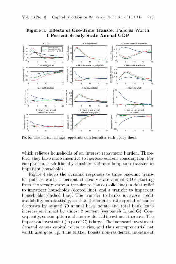
Figure 4. Effects of One-Time Transfer Policies Worth1 Percent Steady-State Annual GDP
Note: The horizontal axis represents quarters after each policy shock.
which relieves households of an interest repayment burden. There-fore, they have more incentive to increase current consumption. Forcomparison, I additionally consider a simple lump-sum transfer toimpatient households.
Figure 4 shows the dynamic responses to three one-time trans-fer policies worth 1 percent of steady-state annual GDP startingfrom the steady state: a transfer to banks (solid line), a debt reliefto impatient households (dotted line), and a transfer to impatienthouseholds (dashed line). The transfer to banks increases creditavailability substantially, so that the interest rate spread of banksdecreases by around 70 annual basis points and total bank loansincrease on impact by almost 2 percent (see panels L and G). Con-sequently, consumption and non-residential investment increase. Theimpact on investment (in panel C) is large. The increased investmentdemand causes capital prices to rise, and thus entrepreneurial networth also goes up. This further boosts non-residential investment

250 International Journal of Central Banking September 2017
in the subsequent periods. In contrast, the impact on aggregate con-sumption is fairly mild. The consumption of impatient householdsgradually increases partly due to mortgage adjustment costs andis mostly offset in the aggregate by a decrease in the consumptionof patient households. Housing prices decline as patient householdsreduce their demand for housing services due to negative wealtheffects. The effects on inflation are negligible and thus the centralbank raises the nominal rate only a little.
Overall, real GDP increases by 0.17 percent before slowly return-ing to its long-term level. The output effects are quite persistent:GDP increases by 0.14 percent for each of the first two years andby 0.08 percent for the third year. The cumulative output increaseafter ten years amounts to roughly 0.6 percent relative to the baselineannual GDP.
I now turn to evaluating a policy to reduce the debt of impatienthouseholds with funds raised from patient households. The marginalpropensity to consume of the impatient households is higher thanthat of the patient households due to a lower discounting factor, sothat a simple transfer, by itself, can lead to an increase in aggregateconsumption. The dashed line shows the simulation outcomes withthe lump-sum transfer to impatient households. Yet, the debt reliefhas an additional channel to increase consumption. The reductionin existing debt results in a lower funding cost for new home mort-gages through the decreased mortgage default risk. The lending ratespread of home mortgages decreases on impact by 20 annual basispoints, which is 2 basis points larger relative to those under thepolicy with a simple transfer. Consequently, aggregate consumptionincreases initially by 0.3 percent and then goes up by 0.43 percentin the next period, which is 0.05 percent higher than with the policyusing a simple transfer.
However, this sharp boost in consumption leads to a rise in infla-tion. In response to such an inflationary development, the centralbank raises the nominal interest rate, which translates into a rise inthe real interest rate due to price rigidities. A higher real rate causespatient households to cut back on consumption further, so that tenquarters after the policy is undertaken, aggregate consumption fallsbelow its steady state (see panel B). It also leads entrepreneurs torefrain from investment (in panel C) and thus non-residential capital

Vol. 13 No. 3 Capital Injection to Banks vs. Debt Relief to HHs 251
prices decline (in panel E). It is particularly interesting to see thathousing prices (in panel D) decline more under debt relief than undercapital injections to banks, even though debt relief increases theimpatient households’ appetite for housing services. This is becauseunder this policy, patient households reduce housing demand to agreater extent due to higher real interest rates in addition to negativewealth effects.
Overall, real GDP increases sharply by nearly 0.3 percent in thefirst year and then slows down to 0.1 percent in the second year.Then it falls below the steady state and turns negative in the thirdyear and thereafter returns to the non-policy path. In the case ofthe policy with a simple transfer, stimulative output effects are moreshort-lived. The cumulative increase in output after ten years reaches0.45 percent over baseline annual GDP.
To sum up, the output effects of a debt relief to credit-constrainedhouseholds are roughly twice as large as those after injectingresources to banks in the first year. However, the latter dominatesthe former from the second year onward, thereby making a trans-fer to banks more effective over the long run. It is because sucha transfer causes non-residential investment to increase, expand-ing production capacity and thereby resulting in lower inflation.On the contrary, household debt relief gives rise to higher infla-tion and therefore leads to the central bank’s reaction to raise theinterest rate, which significantly dampens investment as well as theconsumption of credit-unconstrained households.
4.2 An Application to the U.S. Housing Debt Crisis
4.2.1 The Effects of the Collapse in Housing Prices
In this subsection I analyze the effects of the sharp decline in houseprices observed in the U.S. subprime mortgage crisis. House pricesstarted to decline from the first half of 2006, long before the reces-sion began, and plummeted until the second quarter of 2009. Thenthey remained more or less flat until 2011 before they started torecover. Based on the S&P Case-Shiller U.S. National Home PriceIndex adjusted by the implicit GDP deflator, house prices droppedby around 30 percent from 2006:Q1 to 2009:Q2. If the stochastic

252 International Journal of Central Banking September 2017
trend is removed, house prices declined by nearly 37 percent relativeto the long-run trend over the same periods.39
To engineer such a fall in housing prices, I feed a series of negativehousing preference shocks into the model, similarly to the approachtaken by Justiniano, Primiceri, and Tambalotti (2015). This strat-egy to generate the decline in housing prices is based on severalstudies which, using an estimated structural model with housing,document that shocks on housing preferences are the primary deter-minant of fluctuations in housing prices. Liu, Wang, and Zha (2013)show that housing preference shocks explain around 90 percent offluctuations in housing prices at all the different forecasting hori-zons from one quarter to six years.40 Also, Guerrieri and Iacoviello(2015a) find that the decline in housing prices observed during theGreat Recession is almost exclusively explained by the realizationsof housing preference shocks.41 Therefore, this exercise allows usto quantify the isolated effects of the observed decline in housingprices on macroeconomic aggregates as well as the relevant financialvariables.
Figure 5 presents the model-simulated outcomes together withtheir analogous data observed from the first quarter of 2006 to thefourth quarter of 2014. The actual data include GDP, consumption,
39I use a one-sided Hodrick-Prescott (HP) filter with a value of λ = 100,000 todecompose a time series into a trend component and a cycle component. Guerrieriand Iacoviello (2015a) argue that choosing high λ produces plausible estimates formacroeconomic aggregates and financial variables during the Great Recession. Inaddition, the one-sided filter prevents the decomposition from being influenced bythe correlation between the current observation and the subsequent observations.
40The finding is based on variance decompositions reported in table 3 of Liu,Wang, and Zha (2013). Their model includes a representative patient house-hold and a representative impatient entrepreneur. The entrepreneur’s borrow-ing is tied to the value of collateral assets consisting of commercial real estateand non-residential capital. The model employs eight exogenous shock processes:an intertemporal preference shock, a housing preference shock, a labor supplyshock, permanent and transitory technology shocks, permanent and transitoryinvestment-specific shocks, and a collateral shock.
41The results are obtained from historical decompositions presented in figure 5of Guerrieri and Iacoviello (2015a). The model includes patient households andimpatient households. The debt of impatient households is occasionally tied totheir housing value. The model uses six exogenous shock processes: an intertem-poral preference shock, a housing preference shock, a price markup shock, a wagemarkup shock, an investment shock, and a monetary policy shock.
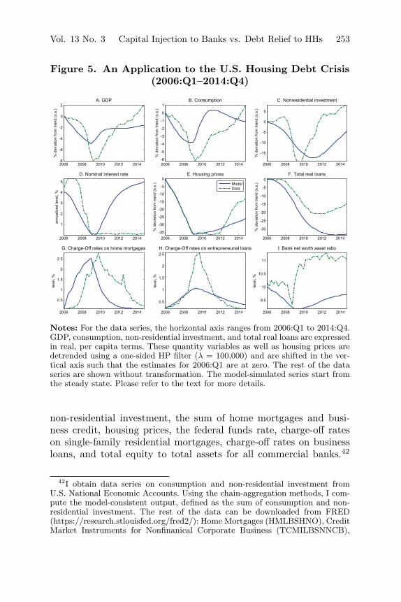
Vol. 13 No. 3 Capital Injection to Banks vs. Debt Relief to HHs 253
Figure 5. An Application to the U.S. Housing Debt Crisis(2006:Q1–2014:Q4)
Notes: For the data series, the horizontal axis ranges from 2006:Q1 to 2014:Q4.GDP, consumption, non-residential investment, and total real loans are expressedin real, per capita terms. These quantity variables as well as housing prices aredetrended using a one-sided HP filter (λ = 100,000) and are shifted in the ver-tical axis such that the estimates for 2006:Q1 are at zero. The rest of the dataseries are shown without transformation. The model-simulated series start fromthe steady state. Please refer to the text for more details.
non-residential investment, the sum of home mortgages and busi-ness credit, housing prices, the federal funds rate, charge-off rateson single-family residential mortgages, charge-off rates on businessloans, and total equity to total assets for all commercial banks.42
42I obtain data series on consumption and non-residential investment fromU.S. National Economic Accounts. Using the chain-aggregation methods, I com-pute the model-consistent output, defined as the sum of consumption and non-residential investment. The rest of the data can be downloaded from FRED(https://research.stlouisfed.org/fred2/): Home Mortgages (HMLBSHNO), CreditMarket Instruments for Nonfinanical Corporate Business (TCMILBSNNCB),
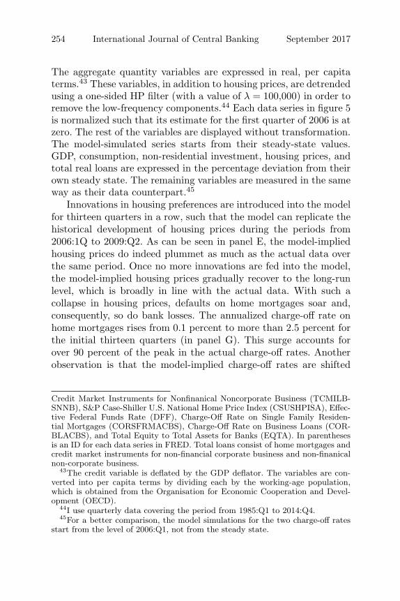
254 International Journal of Central Banking September 2017
The aggregate quantity variables are expressed in real, per capitaterms.43 These variables, in addition to housing prices, are detrendedusing a one-sided HP filter (with a value of λ = 100,000) in order toremove the low-frequency components.44 Each data series in figure 5is normalized such that its estimate for the first quarter of 2006 is atzero. The rest of the variables are displayed without transformation.The model-simulated series starts from their steady-state values.GDP, consumption, non-residential investment, housing prices, andtotal real loans are expressed in the percentage deviation from theirown steady state. The remaining variables are measured in the sameway as their data counterpart.45
Innovations in housing preferences are introduced into the modelfor thirteen quarters in a row, such that the model can replicate thehistorical development of housing prices during the periods from2006:1Q to 2009:Q2. As can be seen in panel E, the model-impliedhousing prices do indeed plummet as much as the actual data overthe same period. Once no more innovations are fed into the model,the model-implied housing prices gradually recover to the long-runlevel, which is broadly in line with the actual data. With such acollapse in housing prices, defaults on home mortgages soar and,consequently, so do bank losses. The annualized charge-off rate onhome mortgages rises from 0.1 percent to more than 2.5 percent forthe initial thirteen quarters (in panel G). This surge accounts forover 90 percent of the peak in the actual charge-off rates. Anotherobservation is that the model-implied charge-off rates are shifted
Credit Market Instruments for Nonfinanical Noncorporate Business (TCMILB-SNNB), S&P Case-Shiller U.S. National Home Price Index (CSUSHPISA), Effec-tive Federal Funds Rate (DFF), Charge-Off Rate on Single Family Residen-tial Mortgages (CORSFRMACBS), Charge-Off Rate on Business Loans (COR-BLACBS), and Total Equity to Total Assets for Banks (EQTA). In parenthesesis an ID for each data series in FRED. Total loans consist of home mortgages andcredit market instruments for non-financial corporate business and non-finanicalnon-corporate business.
43The credit variable is deflated by the GDP deflator. The variables are con-verted into per capita terms by dividing each by the working-age population,which is obtained from the Organisation for Economic Cooperation and Devel-opment (OECD).
44I use quarterly data covering the period from 1985:Q1 to 2014:Q4.45For a better comparison, the model simulations for the two charge-off rates
start from the level of 2006:Q1, not from the steady state.
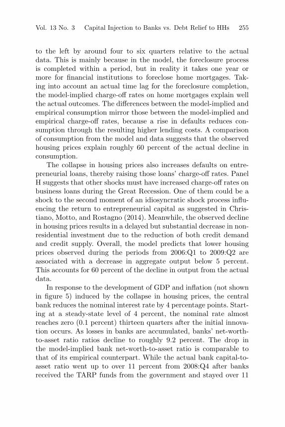
Vol. 13 No. 3 Capital Injection to Banks vs. Debt Relief to HHs 255
to the left by around four to six quarters relative to the actualdata. This is mainly because in the model, the foreclosure processis completed within a period, but in reality it takes one year ormore for financial institutions to foreclose home mortgages. Tak-ing into account an actual time lag for the foreclosure completion,the model-implied charge-off rates on home mortgages explain wellthe actual outcomes. The differences between the model-implied andempirical consumption mirror those between the model-implied andempirical charge-off rates, because a rise in defaults reduces con-sumption through the resulting higher lending costs. A comparisonof consumption from the model and data suggests that the observedhousing prices explain roughly 60 percent of the actual decline inconsumption.
The collapse in housing prices also increases defaults on entre-preneurial loans, thereby raising those loans’ charge-off rates. PanelH suggests that other shocks must have increased charge-off rates onbusiness loans during the Great Recession. One of them could be ashock to the second moment of an idiosyncratic shock process influ-encing the return to entrepreneurial capital as suggested in Chris-tiano, Motto, and Rostagno (2014). Meanwhile, the observed declinein housing prices results in a delayed but substantial decrease in non-residential investment due to the reduction of both credit demandand credit supply. Overall, the model predicts that lower housingprices observed during the periods from 2006:Q1 to 2009:Q2 areassociated with a decrease in aggregate output below 5 percent.This accounts for 60 percent of the decline in output from the actualdata.
In response to the development of GDP and inflation (not shownin figure 5) induced by the collapse in housing prices, the centralbank reduces the nominal interest rate by 4 percentage points. Start-ing at a steady-state level of 4 percent, the nominal rate almostreaches zero (0.1 percent) thirteen quarters after the initial innova-tion occurs. As losses in banks are accumulated, banks’ net-worth-to-asset ratio ratios decline to roughly 9.2 percent. The drop inthe model-implied bank net-worth-to-asset ratio is comparable tothat of its empirical counterpart. While the actual bank capital-to-asset ratio went up to over 11 percent from 2008:Q4 after banksreceived the TARP funds from the government and stayed over 11

256 International Journal of Central Banking September 2017
percent, the model predicts a fairly gradual returning to the long-runlevel. These differences occur mainly due to the model’s inability toaccount for the post-crisis government responses and their impacton the value of banks’ marketable assets. As for total real loans, wefind that the deleveraging implied by the model is much faster thanwhat had happened during the Great Recession.
4.2.2 Policy Experiments in the Middle of the U.S. HousingDebt Crisis
As presented in the introduction, the U.S. government used about$500 billion to recapitalize the U.S. financial system. This amountof funds corresponds to 4.2 percent of the sum of 2008 annual con-sumption and non-residential investment. In this subsection, I ana-lyze the effects of this recapitalization program and compare themwith those of a debt relief program providing the same amount offunds. With the observation that almost all of the funds to sup-port the financial sector were disbursed or committed in one ortwo quarters after the Troubled Assets Relief Program (TARP)was set up in September 2008, I model a policy intervention as aone-time unexpected shock, namely, a one-shot transfer worth 4.2percent of annual GDP (consumption + non-residential investment)from patient households to either banks or impatient households.46
To focus on the effects caused by the policies, I abstract from adistortionary fiscal policy and assume that Ricardian equivalenceholds.47
The results from the preceding policy exercises in normal times(in section 4.1.3) imply that the bank recapitalization of 4.2 percentof annual GDP would increase GDP by nearly 1.2 percent for thefirst two years, and by 1.3 percent for the next eight years. In thecase of the debt relief to impatient households, GDP would increase
46Ninety-nine percent of the TARP funds used to support the financial sectorwas disbursed or pledged from 2008:Q4 to 2009:Q1. The maximum commitmentto rescuing Fannie Mae and Freddie Mac was initially announced in 2008:Q4 andwas revised once in 2009:Q1.
47All lump-sum taxes are assumed to be paid by patient households. As theybehave according to the permanent income hypothesis, the timing of taxes isirrelevant for their consumption-saving decisions.

Vol. 13 No. 3 Capital Injection to Banks vs. Debt Relief to HHs 257
by 1.5 percent for the initial two years, followed by a mild increase(0.4 percentage points) for the next eight years.48
These policy effects are simulated as a deviation from the model’ssteady state. Obviously, the U.S. economy was in the midst ofsevere financial turbulence when government funds were injectedinto financial institutions. Since a log-linearized version of the modelis used for the simulation, a simple transfer policy would bring aboutidentical results regardless of where the simulation starts. However,the effects of a debt relief can be different even in a linear model dueto the introduction of default risk. The impatient households’ deci-sion whether to default or not depends on their outstanding debt.The amount of existing debt at any period during the simulation isnot necessarily the same because it is endogenously determined aspart of the equilibrium. On top of that, the federal fund rates haveremained near zero since 2008:Q4. Taking into account that the fed-eral fund rates are constrained at the zero lower bound (ZLB) cancreate additional non-linear effects on the economy. The subsequentexperiments deal with these two considerations.
I again use the previous crisis experiment for evaluating theeffects of the two policies. To measure policy effects I simulate themodel with and without a policy shock and compute the differencesin simulation outcomes. More precisely, I first compute the modelimplications only with a series of negative housing preference shocks,and then compute the model implications with an additional policyshock in 2009:Q1 (the twelfth quarter).
Figure 6 depicts the effects of bank recapitalization (solid line)versus household debt relief (dotted line) in the middle of the U.S.housing debt crisis. The left column shows the policy effects with-out the consideration of the ZLB. The vertical line indicates theperiod when the policy action is undertaken. The effects of house-hold debt relief on consumption are striking. The debt relief increasesconsumption more than 3 percentage points relative to the consump-tion level that would prevail without the policy. In the experimentstarting from the steady state, the same policy raises consumptionup to around 1.8 percentage points, which is far below 3 percentagepoints. As shown in panel G of figure 5, charge-off rates on home
48Policy effects are computed by just multiplying the simulation outcomes givenin figure 4 with the relative magnitude of the policy (4.2).

258 International Journal of Central Banking September 2017
Figure 6. Effects of Bank Recapitalization versusHoushold Debt Relief Worth 4.2 Percent of Annual GDP
in the Middle of the U.S. Housing Debt Crisis
Notes: The simulations start from the steady state. The vertical axis representsthe differences in model implications with a policy shock and those without apolicy shock. The vertical line in the twelfth quarter indicates the period when apolicy action is undertaken. Please refer to the text for more details.
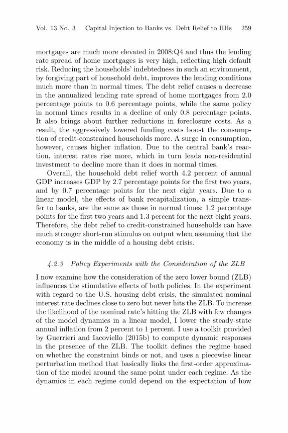
Vol. 13 No. 3 Capital Injection to Banks vs. Debt Relief to HHs 259
mortgages are much more elevated in 2008:Q4 and thus the lendingrate spread of home mortgages is very high, reflecting high defaultrisk. Reducing the households’ indebtedness in such an environment,by forgiving part of household debt, improves the lending conditionsmuch more than in normal times. The debt relief causes a decreasein the annualized lending rate spread of home mortgages from 2.0percentage points to 0.6 percentage points, while the same policyin normal times results in a decline of only 0.8 percentage points.It also brings about further reductions in foreclosure costs. As aresult, the aggressively lowered funding costs boost the consump-tion of credit-constrained households more. A surge in consumption,however, causes higher inflation. Due to the central bank’s reac-tion, interest rates rise more, which in turn leads non-residentialinvestment to decline more than it does in normal times.
Overall, the household debt relief worth 4.2 percent of annualGDP increases GDP by 2.7 percentage points for the first two years,and by 0.7 percentage points for the next eight years. Due to alinear model, the effects of bank recapitalization, a simple trans-fer to banks, are the same as those in normal times: 1.2 percentagepoints for the first two years and 1.3 percent for the next eight years.Therefore, the debt relief to credit-constrained households can havemuch stronger short-run stimulus on output when assuming that theeconomy is in the middle of a housing debt crisis.
4.2.3 Policy Experiments with the Consideration of the ZLB
I now examine how the consideration of the zero lower bound (ZLB)influences the stimulative effects of both policies. In the experimentwith regard to the U.S. housing debt crisis, the simulated nominalinterest rate declines close to zero but never hits the ZLB. To increasethe likelihood of the nominal rate’s hitting the ZLB with few changesof the model dynamics in a linear model, I lower the steady-stateannual inflation from 2 percent to 1 percent. I use a toolkit providedby Guerrieri and Iacoviello (2015b) to compute dynamic responsesin the presence of the ZLB. The toolkit defines the regime basedon whether the constraint binds or not, and uses a piecewise linearperturbation method that basically links the first-order approxima-tion of the model around the same point under each regime. As thedynamics in each regime could depend on the expectation of how
260 International Journal of Central Banking September 2017
long the economy stays in that regime, the simulation outcomes canbe highly non-linear.
As in the previous policy experiment, I feed in each policy shockin the twelfth quarter. Without any policy, the nominal interestrate would stay at zero for five quarters more until the sixteenthquarter.49 Figure 6 presents the simulation results for GDP, con-sumption, investment, and the nominal interest rate without theZLB on the left and with the ZLB on the right. First of all, theoutput effects of both policies are bigger when the nominal interestrate is constrained at zero than in the other case. The peak out-put effect of the transfer to banks under the ZLB is approximately1.0 percentage point, which is around 40 percent higher than thatwithout the ZLB (0.7 percentage point). The peak output effect ofthe debt relief to impatient households under the ZLB is roughly4.0 percentage points, which is nearly 70 percent higher than thatof normal times (2.4 percentage points). Second, each policy helpsthe economy to escape from a liquidity trap one quarter earlier. Thenominal interest rate is constrained at zero for one year until the fif-teenth quarter and thereafter it is set according to the interest raterule. Third, the stimulative effects of the debt relief are magnifiedunder the ZLB. The debt relief is inflationary, so that the real inter-est rate falls, when the nominal interest rate cannot go below zero.The decrease in real interest rates in turn boosts consumption ofboth households as well as non-residential investment, and at leastweakens crowding-out effects.
Overall, a debt relief worth 4.2 percent of annual GDP increasesannual GDP by 5.2 percentage points for the first two years. Theseoutput effects are far beyond those of bank recapitalization (1.6percentage points). For the next eight years, the debt relief wouldincrease GDP by 2.0 percent, whereas the bank capitalization boostsGDP by 1.5 percent. These results suggest that the debt relief pol-icy under the ZLB has far-reaching effects on the economy beyondthe periods during which the nominal interest rate is constrained at
49The nominal interest rate is endogenously kept at zero for two years fromthe ninth to the sixteenth quarter. Since the ZLB prevents the nominal interestrate from falling down to the level at which efficient intertemporal allocationscan be made, aggregate demand consisting of consumption and non-residentialinvestment decreases further than without the ZLB. The discussion and figuresare presented in Yoo (2017).
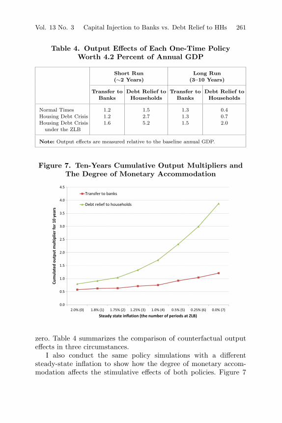
Vol. 13 No. 3 Capital Injection to Banks vs. Debt Relief to HHs 261
Table 4. Output Effects of Each One-Time PolicyWorth 4.2 Percent of Annual GDP
Short Run Long Run(∼2 Years) (3–10 Years)
Transfer to Debt Relief to Transfer to Debt Relief toBanks Households Banks Households
Normal Times 1.2 1.5 1.3 0.4Housing Debt Crisis 1.2 2.7 1.3 0.7Housing Debt Crisis 1.6 5.2 1.5 2.0
under the ZLB
Note: Output effects are measured relative to the baseline annual GDP.
Figure 7. Ten-Years Cumulative Output Multipliers andThe Degree of Monetary Accommodation
zero. Table 4 summarizes the comparison of counterfactual outputeffects in three circumstances.
I also conduct the same policy simulations with a differentsteady-state inflation to show how the degree of monetary accom-modation affects the stimulative effects of both policies. Figure 7
262 International Journal of Central Banking September 2017
presents the cumulative output multipliers of each policy for tenyears—the line with squares for the transfer to banks and the linewith triangles for the debt relief to households—at each steady-stateinflation. Following Uhlig (2010), the cumulative multiplier is definedas a ratio whose numerator equals the present values of policy-induced output effects relative to the steady state for ten years,and whose denominator equals the size of the policy measure, whichin this case is 4.2 percent of annual steady-state GDP. I assume zerodiscount rates, namely, making a simple sum of policy-induced out-put effects.50 The number in the parentheses on the x-axis indicateshow many quarters the nominal interest rates are stuck at zero fromthe period of the policy intervention. As can be seen, the longer thepolicy rates are constrained at the ZLB, the higher the cumulativeoutput multipliers are for both policies. The cumulative multiplierof capital injection policies is 0.6 when the ZLB is disregarded, butit doubles when the policy rate stays at zero for seven quarters.More interestingly, in the case of debt relief policies, the cumulativemultiplier accelerates as the number of periods that the economy isconstrained at the ZLB increases. The cumulative multiplier whenthe policy rate stays at zero for seven quarters is nearly 4.0, whichis nearly five times as big as that without the ZLB (0.8).
5. Conclusion
In this paper, I build a DSGE model having major macrofinanciallinkages identified in the literature with a particular focus on therole of housing finance. I use the model to analyze the macroeco-nomic effects of a collapse in house prices observed in the recentU.S. housing debt crisis. Then such a crisis environment is used as alaboratory for assessing the relative effectiveness of a policy to injectcapital into banks versus a policy to relieve households of mortgagedebt. The magnitude and timing of each policy are chosen to becomparable to those of financial-sector support programs that theU.S. government conducted during the crisis.
The policy simulation results suggest that policies to supportthe financial sector helped to ease the severity of the recession in
50This is equivalent to the assumption that the discount rates are the same asthe trend growth rates.
Vol. 13 No. 3 Capital Injection to Banks vs. Debt Relief to HHs 263
the aftermath of the housing debt crisis. The more important impli-cation is, however, that debt relief to households of the same amountof funds would have been much more effective to stimulate the econ-omy, given that the household sector was highly leveraged and thenominal interest rates were constrained at the ZLB. Therefore, thispaper supports the view of Mian and Sufi (2014) and others, whoargue for a more aggressive reduction of household debt.51
Despite the detailed model structure, several issues need to beaddressed in order to quantify the effects of household debt reliefmore precisely. First, it would take some time for government agen-cies to undertake the necessary steps to carry out a policy to reducehousehold debt, because such a policy involves a lot of parties unlikethe financial-sector support programs. In my policy experiments,however, the debt relief is modeled as a one-time policy interventionto facilitate a direct comparison with the capital injection to banks.As shown in Cogan et al. (2010), the significant implementation lagof fiscal policy can reduce its stimulative effects. Meanwhile, theanticipation of the scheduled debt relief policy can ameliorate thecurrent credit condition by loosening the participation constraintof banks. In the end, it is a quantitative issue as to which onedominates the other. Second, while the model partly accounts forsluggish mortgage dynamics by introducing loan adjustment costs,the introduction of explicitly defined long-term mortgage contractswould be more desirable. The recent papers by Elenev, Landvoigt,and Nieuwerburgh (2015) and Gelain, Lansing, and Natvik (2015)deal with an interesting modeling setup for long-term mortgage con-tracts. Third, the default decision could be modeled in more detail.For example, by introducing a direct penalty or cost on defaultedagents, an access to credit market would be restricted for a stochas-tic length of periods once borrowers declare default (see Chatterjeeand Eyigungor 2015).
Besides the evaluation of the post-crisis government policies, themodel can be used or extended for analyzing other interesting macro-economic policies. Areas for future research include the design of
51Note that throughout the policy simulations, I implicitly assume that themain driver of the recent housing debt crisis is a shock on house prices. If othershocks, such as a shock originating from the financial sector are considered to bedominant, the relative effectiveness of the policies can be different.
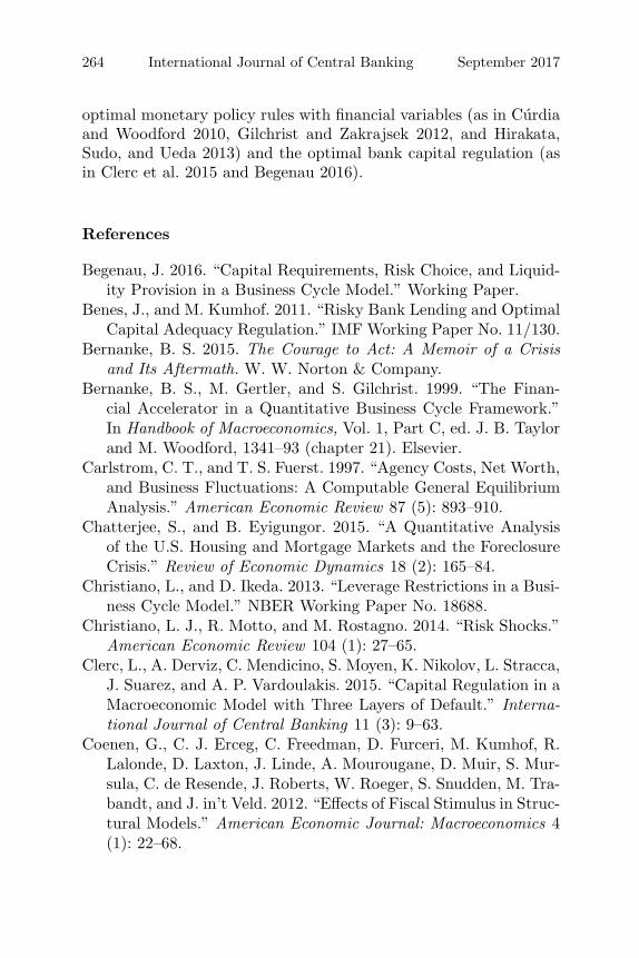
264 International Journal of Central Banking September 2017
optimal monetary policy rules with financial variables (as in Curdiaand Woodford 2010, Gilchrist and Zakrajsek 2012, and Hirakata,Sudo, and Ueda 2013) and the optimal bank capital regulation (asin Clerc et al. 2015 and Begenau 2016).
References
Begenau, J. 2016. “Capital Requirements, Risk Choice, and Liquid-ity Provision in a Business Cycle Model.” Working Paper.
Benes, J., and M. Kumhof. 2011. “Risky Bank Lending and OptimalCapital Adequacy Regulation.” IMF Working Paper No. 11/130.
Bernanke, B. S. 2015. The Courage to Act: A Memoir of a Crisisand Its Aftermath. W. W. Norton & Company.
Bernanke, B. S., M. Gertler, and S. Gilchrist. 1999. “The Finan-cial Accelerator in a Quantitative Business Cycle Framework.”In Handbook of Macroeconomics, Vol. 1, Part C, ed. J. B. Taylorand M. Woodford, 1341–93 (chapter 21). Elsevier.
Carlstrom, C. T., and T. S. Fuerst. 1997. “Agency Costs, Net Worth,and Business Fluctuations: A Computable General EquilibriumAnalysis.” American Economic Review 87 (5): 893–910.
Chatterjee, S., and B. Eyigungor. 2015. “A Quantitative Analysisof the U.S. Housing and Mortgage Markets and the ForeclosureCrisis.” Review of Economic Dynamics 18 (2): 165–84.
Christiano, L., and D. Ikeda. 2013. “Leverage Restrictions in a Busi-ness Cycle Model.” NBER Working Paper No. 18688.
Christiano, L. J., R. Motto, and M. Rostagno. 2014. “Risk Shocks.”American Economic Review 104 (1): 27–65.
Clerc, L., A. Derviz, C. Mendicino, S. Moyen, K. Nikolov, L. Stracca,J. Suarez, and A. P. Vardoulakis. 2015. “Capital Regulation in aMacroeconomic Model with Three Layers of Default.” Interna-tional Journal of Central Banking 11 (3): 9–63.
Coenen, G., C. J. Erceg, C. Freedman, D. Furceri, M. Kumhof, R.Lalonde, D. Laxton, J. Linde, A. Mourougane, D. Muir, S. Mur-sula, C. de Resende, J. Roberts, W. Roeger, S. Snudden, M. Tra-bandt, and J. in’t Veld. 2012. “Effects of Fiscal Stimulus in Struc-tural Models.” American Economic Journal: Macroeconomics 4(1): 22–68.

Vol. 13 No. 3 Capital Injection to Banks vs. Debt Relief to HHs 265
Cogan, J., T. Cwik, J. Taylor, and V. Wieland. 2010. “New Keyne-sian versus Old Keynesian Government Spending Multipliers.”Journal of Economic Dynamics and Control 34 (3): 281–95.
Covas, F., and J. C. Driscoll. 2014. “Bank Liquidity and CapitalRegulation in General Equilibrium.” Finance and Economics Dis-cussion Series No. 2014-85, Board of Governors of the FederalReserve System.
Curdia, V., and M. Woodford. 2010. “Credit Spreads and MonetaryPolicy.” Journal of Money, Credit and Banking 42 (s1): 3–35.
Dogra, K. 2014. “Liquidity Traps, Debt Relief, and MacroprudentialPolicy: A Mechanism Design Approach.” Working Paper.
Duca, J. V., J. Muellbauer, and A. Murphy. 2011. “House Pricesand Credit Constraints: Making Sense of the US Experience.”Economic Journal 121 (552): 533–51.
Eggertsson, G. B., and P. Krugman. 2012. “Debt, Deleveraging, andthe Liquidity Trap: A Fisher-Minsky-Koo Approach.” QuarterlyJournal of Economics 127 (3): 1469–1513.
Elenev, V., T. Landvoigt, and S. V. Nieuwerburgh. 2015. “PhasingOut the GSEs.” Working Paper.
Forlati, C., and L. Lambertini. 2011. “Risky Mortgages in a DSGEModel.” International Journal of Central Banking 7 (1): 285–335.
Gale, D., and M. Hellwig. 1985. “Incentive-Compatible Debt Con-tracts: The One-Period Problem.” Review of Economic Studies52 (4): 647–63.
Geanakoplos, J. 2010. “The Leverage Cycle.” In NBER Macroeco-nomics Annual 2009, Vol. 24, ed. D. Acemoglu, K. Rogoff, andM. Woodford, 1–65 (chapter 1). University of Chicago Press.
Geithner, T. F. 2014. Stress Test: Reflections on Financial Crises.Crown Publishers.
Gelain, P., K. J. Lansing, and G. J. Natvik. 2015. “Leaning againstthe Credit Cycle.” Working Paper No. 04/2015, Norges Bank.
Gerali, A., S. Neri, L. Sessa, and F. M. Signoretti. 2010. “Credit andBanking in a DSGE Model of the Euro Area.” Journal of Money,Credit and Banking 42 (s1): 107–41.
Gertler, M., and P. Karadi. 2011. “A Model of Unconventional Mon-etary Policy.” Journal of Monetary Economics 58 (1): 17–34.
Gilchrist, S., and E. Zakrajsek. 2012. “Credit Supply Shocksand Economic Activity in a Financial Accelerator Model.” In
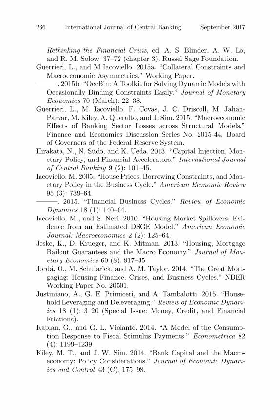
266 International Journal of Central Banking September 2017
Rethinking the Financial Crisis, ed. A. S. Blinder, A. W. Lo,and R. M. Solow, 37–72 (chapter 3). Russel Sage Foundation.
Guerrieri, L., and M Iacoviello. 2015a. “Collateral Constraints andMacroeconomic Asymmetries.” Working Paper.
———. 2015b. “OccBin: A Toolkit for Solving Dynamic Models withOccasionally Binding Constraints Easily.” Journal of MonetaryEconomics 70 (March): 22–38.
Guerrieri, L., M. Iacoviello, F. Covas, J. C. Driscoll, M. Jahan-Parvar, M. Kiley, A. Queralto, and J. Sim. 2015. “MacroeconomicEffects of Banking Sector Losses across Structural Models.”Finance and Economics Discussion Series No. 2015-44, Boardof Governors of the Federal Reserve System.
Hirakata, N., N. Sudo, and K. Ueda. 2013. “Capital Injection, Mon-etary Policy, and Financial Accelerators.” International Journalof Central Banking 9 (2): 101–45.
Iacoviello, M. 2005. “House Prices, Borrowing Constraints, and Mon-etary Policy in the Business Cycle.” American Economic Review95 (3): 739–64.
———. 2015. “Financial Business Cycles.” Review of EconomicDynamics 18 (1): 140–64.
Iacoviello, M., and S. Neri. 2010. “Housing Market Spillovers: Evi-dence from an Estimated DSGE Model.” American EconomicJournal: Macroeconomics 2 (2): 125–64.
Jeske, K., D. Krueger, and K. Mitman. 2013. “Housing, MortgageBailout Guarantees and the Macro Economy.” Journal of Mon-etary Economics 60 (8): 917–35.
Jorda, O., M. Schularick, and A. M. Taylor. 2014. “The Great Mort-gaging: Housing Finance, Crises, and Business Cycles.” NBERWorking Paper No. 20501.
Justiniano, A., G. E. Primiceri, and A. Tambalotti. 2015. “House-hold Leveraging and Deleveraging.” Review of Economic Dynam-ics 18 (1): 3–20 (Special Issue: Money, Credit, and FinancialFrictions).
Kaplan, G., and G. L. Violante. 2014. “A Model of the Consump-tion Response to Fiscal Stimulus Payments.” Econometrica 82(4): 1199–1239.
Kiley, M. T., and J. W. Sim. 2014. “Bank Capital and the Macro-economy: Policy Considerations.” Journal of Economic Dynam-ics and Control 43 (C): 175–98.

Vol. 13 No. 3 Capital Injection to Banks vs. Debt Relief to HHs 267
———. 2015. “Optimal Monetary and Macroprudential Policies:Gains and Pitfalls in a Model of Financial Intermediation.”Finance and Economics Discussion Series No. 2015-78, Boardof Governors of the Federal Reserve System.
Kiyotaki, N., and J. Moore. 1997. “Credit Cycles.” Journal of Polit-ical Economy 105 (2): 211–48.
Kollmann, R., M. Ratto, W. Roeger, and J. in’t Veld. 2013. “FiscalPolicy, Banks and the Financial Crisis.” Journal of EconomicDynamics and Control 37 (2): 387–403 (Special Issue: FiscalPolicy in the Aftermath of the Financial Crisis).
Landvoigt, T. 2014. “The Allocation and Pricing of Mortgage Risk.”Working Paper.
Liu, Z., P. Wang, and T. Zha. 2013. “Land-Price Dynamics andMacroeconomic Fluctuations.” Econometrica 81 (3): 1147–84.
Mian, A., K. Rao, and A. Sufi. 2013. “Household Balance Sheets,Consumption, and the Economic Slump.” Quarterly Journal ofEconomics 128 (4): 1687–1726.
Mian, A., and A. Sufi. 2014. House of Debt: How They (and You)Caused the Great Recession, and How We Can Prevent It fromHappening Again. University of Chicago Press.
Mian, A., A. Sufi, and F. Trebbi. 2015. “Foreclosures, House Prices,and the Real Economy.” Journal of Finance 70 (6): 2587–2634.
Nakamura, E., and J. Steinsson. 2014. “Fiscal Stimulus in a Mon-etary Union: Evidence from US Regions.” American EconomicReview 104 (3): 753–92.
Quint, D., and P. Rabanal. 2014. “Monetary and Macropruden-tial Policy in an Estimated DSGE Model of the Euro Area.”International Journal of Central Banking 10 (2): 169–236.
Reinhart, C., and K. Rogoff. 2009. This Time Is Different: EightCenturies of Financial Folly. Princeton University Press.
Shiller, R. 2012. “Reviving Real Estate Requires Collective Action.”New York Times, June 23.
Smets, F., and R. Wouters. 2007. “Shocks and Frictions in US Busi-ness Cycles: A Bayesian DSGE Approach.” American EconomicReview 97 (3): 586–606.
Stiglitz, J. 2010. “Foreclosures and Banks’ Debt to Society.” TheGuardian, November 5.
Summers, L. 2014. “Lawrence Summers on ‘House of Debt’: Didthe Response to the Financial Crisis Focus Too Much on Banks

268 International Journal of Central Banking September 2017
while Neglecting Over-indebted Homeowners?” Financial Times,June 6.
Uhlig, H. 2010. “Some Fiscal Calculus.” American Economic Review100 (2): 30–34.
van der Kwaak, C., and S. van Wijnbergen. 2014. “FinancialFragility, Sovereign Default Risk and the Limits to CommercialBank Bail-outs.” Journal of Economic Dynamics and Control 43(C): 218–40.
Walentin, K. 2014. “Business Cycle Implications of MortgageSpreads.” Journal of Monetary Economics 67 (C): 62–77.
Whelan, K. 2002. “A Guide to U.S. Chain Aggregated NIPA Data.”Review of Income and Wealth 48 (2): 217–33.
Wieland, V., E. Afanasyeva, M. Kuete, and J. Yoo. 2016. “NewMethods for Macro-Financial Model Comparison and PolicyAnalysis. In Handbook of Macroeconomics, Vol. 2, ed. J. B. Taylorand H. Uhlig, 1241–1319 (chapter 15). Elsevier.
Yoo, J. 2017. “Capital Injection to Banks versus Debt Relief toHouseholds.” IMFS Working Paper No. 111.