can climate-effective land management reduce regional warming? · can climate-effective land...

Can climate-effective land management reduceregional warming?A. L. Hirsch1 , M. Wilhelm1, E. L. Davin1, W. Thiery1,2 , and S. I. Seneviratne1

1Institute for Atmospheric and Climate Science, ETH Zurich, Zurich, Switzerland, 2Department of Hydrology and HydraulicEngineering, Vrije Universiteit Brussel, Brussels, Belgium

Abstract Limiting global warming to well below 2°C is an imminent challenge for humanity. However,even if this global target can be met, some regions are still likely to experience substantial warmingrelative to others. Using idealized global climate simulations, we examine the potential of landmanagement options in affecting regional climate, with a focus on crop albedo enhancement andirrigation (climate-effective land management). The implementation is performed over all crop regionsglobally to provide an upper bound. We find that the implementation of both crop albedo enhancementand irrigation can reduce hot temperature extremes by more than 2°C in North America, Eurasia, and Indiaover the 21st century relative to a scenario without management application. The efficacy of crop albedoenhancement scales with the magnitude, where a cooling response exceeding 0.5°C for hot temperatureextremes was achieved with a large (i.e., ≥0.08) change in crop albedo. Regional differences were attributedto the surface energy balance response with temperature changes mostly explained by latent heat fluxchanges for irrigation and net shortwave radiation changes for crop albedo enhancement. However,limitations do exist, where we identify warming over the winter months when climate-effective landmanagement is temporarily suspended. This was associated with persistent cloud cover that enhanceslongwave warming. It cannot be confirmed if the magnitude of this feedback is reproducible in other climatemodels. Our results overall demonstrate that regional warming of hot extremes in our climate model can bepartially mitigated when using an idealized treatment of climate-effective land management.

1. IntroductionRecent research illustrates that as a consequence of global anthropogenic climate change, some regionswill warm at an accelerated rate relative to the global mean temperature anomaly [Seneviratne et al.,2016]. Despite the recent global commitment to limit global warming to well below 2°C [United NationsFramework Convention on Climate Change, 2015] and to reduce greenhouse gas (GHG) emissions accordingly,some regions will still experience a substantially higher magnitude of warming even for this agreed globalwarming target [Seneviratne et al., 2016]. Consequently, this has severe implications on the ability of theseregions to adapt to climate change.

Climate engineering has been in the research discourse for more than 50 years (see reviews from Keith [2000],Crutzen [2006],Wigley [2006], and Caldeira and Bala [2016]) and is considered by some as a possible means toachieve this 2°C limit [e.g., Keith and Irvine, 2016]. Climate engineering involves the deliberate modification ofthe Earth’s climate system to counteract anthropogenic climate change [Intergovernmental Panel on ClimateChange (IPCC), 2013] and can be split between two paradigms: those that involve carbon dioxide removal orchanges in the Earth’s radiation balance. Most carbon dioxide removal concepts are also associated withconventional mitigation activities that can involve carbon sequestration from reforestation and afforestation[e.g., Sonntag et al., 2016]. Proposed schemes altering the radiation balance include, solar reduction geoen-gineering [Irvine et al., 2010; Schaller et al., 2014; Cao et al., 2016], stratospheric aerosol injection [Robock et al.,2008; Jones et al., 2010; Tjiputra et al., 2016], marine cloud brightening [Jones et al., 2009; Muri et al., 2015],cirrus cloud thinning [Kristjansson et al., 2015], desert albedo modification [Irvine et al., 2011; Crook et al.,2015], ocean albedo modification [Crook et al., 2016; Gabriel et al., 2017], and crop albedo modification[Singarayer et al., 2009; Davin et al., 2014; Wilhelm et al., 2015]. Using idealized simulations with EarthSystem Models (ESMs), the Geoengineering Model Intercomparison Project (GeoMIP) [Kravitz et al., 2011,2013a, 2013b, 2015] examines the efficacy of various climate engineering schemes to negate warminginduced by higher GHG concentrations. For example, the GeoMIP G1 experiment [Kravitz et al., 2011] illu-strated that climate engineering via solar reduction geoengineering can reverse the warming associated

HIRSCH ET AL. CLIMATE-EFFECTIVE LAND MANAGEMENT 1

PUBLICATIONSJournal of Geophysical Research: Atmospheres

RESEARCH ARTICLE10.1002/2016JD026125

Key Points:• Crop albedo enhancement andirrigation are more effective atreducing hot temperature extremesthan mean temperature

• Using irrigation with crop albedoenhancement produces the mostrobust cooling response

• Regional differences exist and are afunction of changes in the surfaceenergy balance triggered byclimate-effective land management

Supporting Information:• Supporting Information S1

Correspondence to:A. L. Hirsch and S. I. Seneviratne,[email protected];[email protected]

Citation:Hirsch, A. L., M. Wilhelm, E. L. Davin,W. Thiery, and S. I. Seneviratne (2017),Can climate-effective landmanagementreduce regional warming?, J. Geophys.Res. Atmos., 122, doi:10.1002/2016JD026125.

Received 21 OCT 2016Accepted 11 FEB 2017Accepted article online 14 FEB 2017

©2017. The Authors.This is an open access article under theterms of the Creative CommonsAttribution-NonCommercial-NoDerivsLicense, which permits use and distri-bution in any medium, provided theoriginal work is properly cited, the use isnon-commercial and no modificationsor adaptations are made.

http://orcid.org/0000-0002-5811-2465

http://orcid.org/0000-0002-5183-6145

http://orcid.org/0000-0001-9528-2917

http://publications.agu.org/journals/

http://onlinelibrary.wiley.com/journal/10.1002/(ISSN)2169-8996

http://dx.doi.org/10.1002/2016JD026125

http://dx.doi.org/10.1002/2016JD026125

http://dx.doi.org/10.1002/2016JD026125

http://dx.doi.org/10.1002/2016JD026125

http://dx.doi.org/10.1002/2016JD026125

mailto:[email protected]


with a quadrupling of carbon dioxide concentration; however, the corresponding response of the hydrologi-cal cycle suggests possible negative consequences for several regions [Kravitz et al., 2013b; Tilmes et al., 2013].

Comparisons across different climate engineering schemes are few [e.g., Lenton and Vaughan, 2009; Vaughanand Lenton, 2011; Irvine et al., 2011; Niemeier et al., 2013; Crook et al., 2015; Irvine et al., 2016]. However, Crooket al. [2015] examined the surface temperature and precipitation response of six climate engineeringschemes using single realizations from an ESM. They found that solar reduction geoengineering, marinecloud brightening, cirrus cloud thinning, and ocean albedo modification were the most effective at inducingglobal cooling of the planet of the order of 1°C. Desert albedo modification was found to induce substantialchanges in global circulation and the hydrological cycle, similar to results reported by Irvine et al. [2011].Crook et al. [2015] also examined the potential of crop albedo enhancement but found the effect on meantemperature to be negligible relative to the other climate engineering schemes that they evaluated. Theyalso identify a rapid warming at the termination of all climate engineering schemes except for crop albedoenhancement, as it has no strong cooling effect globally. This imposes an ethical constraint on climateengineering, where the commencement of most schemes requires the long-term commitment of future gen-erations to the continuation of climate engineering to avoid the consequences of sudden termination [e.g.,Jones et al., 2013]. This is particularly true if one adopts an “all or nothing” approach to climate engineering[Keith and Irvine, 2016]. Despite the comparatively limited efficacy of crop albedo enhancement in contrastto other climate engineering schemes reported in the literature, it has some advantages. This includes usingexisting agricultural management techniques and therefore can be considered as a supplement to existingland management practice.

Climate-effective land management (CeLM) considers more than just crop albedo enhancement and caninvolve a diverse range of existing land management practices including double cropping, crop dusting,conservation tillage, forest management, and irrigation [Lobell et al., 2006;Wilhelm et al., 2015]. Most of thesepractices are currently used in agricultural landscapes, with almost two thirds of the global land surfacealready under a substantial level of management [Luyssaert et al., 2014].

The impact of various land management practices on surface climate has been examined before [e.g., Lobellet al., 2006; Ridgwell et al., 2009; Doughty et al., 2011; Irvine et al., 2011; Davin et al., 2014;Wilhelm et al., 2015].Using idealized ESM simulations, Lobell et al. [2006] examine the mean temperature response to irrigation,no-till management, second-growing season, and double cropping under present-day GHG concentrations.All schemes were found to have a regional cooling effect, with irrigation having the largest global coolingeffect on mean temperature of 1.3°C over land. Ridgwell et al. [2009] extended this to consider the efficacyof different levels of crop albedo enhancement under elevated CO2 concentrations. They also find thatincreasing crop albedo can lead to more than 1°C cooling of mean summertime temperatures over agricul-tural landscapes. However, both studies focus on the potential of CeLM schemes to cool mean temperaturewith no examination of what this means for extreme temperatures.

Using a regional climate model to simulate present-day climate, Davin et al. [2014] examine the potential ofno tillage to cool surface climate over Europe. They find an amplified cooling effect on temperature extremesrelative to means. This approach was extended byWilhelm et al. [2015] to consider albedo enhancement overall vegetation types to mitigate temperature extremes for present and future climate. They find thatdecreases in daily maximum temperature (TMAX) scale linearly with the magnitude of albedo enhancementwith strong preferential cooling of hot extremes over the northern midlatitudes during boreal summer(June–August: JJA). Wilhelm et al. [2015] also show that the spatial extent of albedo enhancement is criticalfor the magnitude of cooling at the global scale. In particular, reducing the spatial extent of albedo enhance-ment to agricultural regions and the temporal extent to boreal summer showed smaller changes in TMAX.

In this paper we use idealized ESM simulations to examine the efficacy of CeLM to reduce regional warmingof hot extremes associated with future anthropogenic climate change. By considering the impact of differentCeLM schemes on projected changes in temperature extremes with anthropogenic climate change, wedifferentiate our research from that of Lobell et al. [2006] and Ridgwell et al. [2009]. We extend the approachof Davin et al. [2014] andWilhelm et al. [2015] to compare the efficacy of crop albedo enhancement, irrigation,and the application of both schemes. To our knowledge we are the first study to examine the combinedeffect of crop albedo enhancement and irrigation. We note that the experiments are idealized and that theyare a global implementation of crop albedo enhancement and irrigation. In reality, such modifications are

Journal of Geophysical Research: Atmospheres 10.1002/2016JD026125


more likely to occur at a regional scale, and therefore, our experiment provides an upper bound on what ispossible with CeLM. Finally, we aim to identify regions where particular CeLM schemes are more effectiveand determine whether differences in regional responses are associated with how CeLM affects the surfaceenergy balance.

2. Methods2.1. Model Description

We use the Community Earth System Model version 1.2 [Hurrell et al., 2013], a state-of-the-art climate modelthat consists of component models representing the atmosphere, land, ocean, sea ice, land ice, and theirinteractions. This climate model has been extensively evaluated [e.g., Gent et al., 2011; Hurrell et al., 2013;Meehl et al., 2013] and has been used to examine research questions on climate engineering [e.g., Lobellet al., 2006; Wilhelm et al., 2015; Xia et al., 2016], climate extremes [e.g., Fischer et al., 2013; Perkins andFischer, 2013], and irrigation [e.g., Sacks et al., 2009; Thiery et al., 2017].

The Community Earth System Model can be configured with different versions of the component models.We use the component set B20TRC5CN for the historical period 1850 to 2005 and BRCP85C5CN for the pro-jections starting in 2006. More specifically, we use the Community Atmosphere Model version 5 [Neale et al.,2012] with 48 vertical levels, a time step of 1800s, and a horizontal resolution of 1.9° × 2.5°. The CommunityAtmosphere Model uses a finite volume dynamical core with terrain following hybrid sigma-pressure coordi-nates. Both ozone and volcanic aerosols are prescribed. Transient GHG emissions are used for all simulations,using historical emissions up to 2005 (atmospheric CO2: 285 ppm to 379 ppm) and follow the RepresentativeConcentration Pathway (RCP) 8.5 from 2006 onward (atmospheric CO2: 380 ppm to 936 ppm). The ParallelOcean Program version 2 is used to simulate ocean dynamics with 60 vertical levels and an hourly time stepon a 1° × 1° Greenland-displaced polar grid. By using a fully coupled ESM, we are able to evaluate the effect ofCeLM to counteract global warming.

The Community Land Model version 4 [Oleson et al., 2010; Lawrence et al., 2011] is used with the prognosticcarbon-nitrogen biogeochemical model [Thornton et al., 2007] to represent the terrestrial processes thataffect and are affected by climate through the exchange of energy andmoisture between the land and atmo-spheric components of the Community Earth System Model. With the carbon-nitrogen submodel, the leafand stem area indices and vegetation heights are calculated prognostically, and therefore, vegetation phe-nology is dynamic. Plant functional type (PFT) specific leaf growth and litterfall are a function of the daylength and on the growing degree days exceeding critical temperature and moisture thresholds. There are15 soil layers with increasing layer thicknesses from 0.018m at the surface to 13.9m for the deepest layer.Only the upper 10 layers are hydrologically active using a modified Richard’s equation, while the bottom fivelayers are thermal slabs. To resolve the land surface heterogeneity, a subgrid tiling approach is used, whereeach grid cell is split into different land units to represent vegetated, urban, lake, wetland, and glacial sur-faces. For vegetated surfaces, a single soil column is used, where up to 15 PFTs can coexist, each with theirown set of parameters describing the optical, morphological, and photosynthetic properties of the vegeta-tion class. The same atmospheric conditions are used to drive the land surface model for each land unitand PFT within the grid cell. The surface turbulent energy fluxes, radiative temperature, and albedo variablesare calculated for each PFT and land unit independently before being aggregated to the grid cell level usingthe percent coverage of the grid cell to calculate a weighted average. In all simulations we use historical andprojected transient land cover with land use change descriptions from Hurtt et al. [2006]. We do not use theprognostic crop model to limit computational costs. Furthermore, we do not use the dynamic vegetationmode as this only considers grass and tree PFTs [Lawrence et al., 2011].

The surface albedo is calculated for each PFT at the subgrid level for canopy and soil surfaces separately,which are then aggregated to a total surface albedo estimate as a weighted combination of snow-free andsnow-covered albedos, where the weighting is determined by the snow cover fraction. All albedo termsare modeled using a two-stream approximation for radiative transfer to determine the direct and diffuseradiation contributions. There is also an irrigation parameterization enabled for a generic C3 crop PFT onits own soil column where all parameters are identical to the generic C3 crop PFT [Oleson et al., 2013].Irrigation is only triggered during the growing season and when water is limiting for evapotranspiration.The irrigation rate is calculated as the total water deficit across the topmost unfrozen soil layers. This is



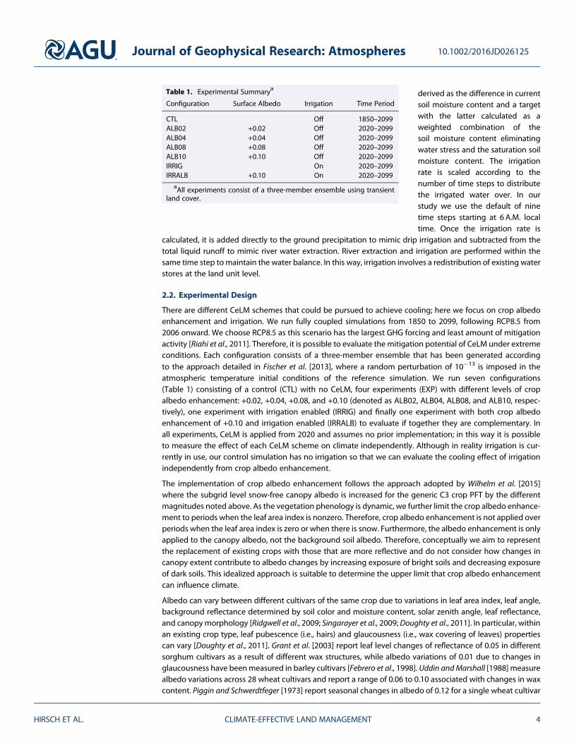
derived as the difference in currentsoil moisture content and a targetwith the latter calculated as aweighted combination of thesoil moisture content eliminatingwater stress and the saturation soilmoisture content. The irrigationrate is scaled according to thenumber of time steps to distributethe irrigated water over. In ourstudy we use the default of ninetime steps starting at 6 A.M. localtime. Once the irrigation rate is

calculated, it is added directly to the ground precipitation to mimic drip irrigation and subtracted from thetotal liquid runoff to mimic river water extraction. River extraction and irrigation are performed within thesame time step tomaintain the water balance. In this way, irrigation involves a redistribution of existing waterstores at the land unit level.

2.2. Experimental Design

There are different CeLM schemes that could be pursued to achieve cooling; here we focus on crop albedoenhancement and irrigation. We run fully coupled simulations from 1850 to 2099, following RCP8.5 from2006 onward. We choose RCP8.5 as this scenario has the largest GHG forcing and least amount of mitigationactivity [Riahi et al., 2011]. Therefore, it is possible to evaluate the mitigation potential of CeLM under extremeconditions. Each configuration consists of a three-member ensemble that has been generated accordingto the approach detailed in Fischer et al. [2013], where a random perturbation of 10�13 is imposed in theatmospheric temperature initial conditions of the reference simulation. We run seven configurations(Table 1) consisting of a control (CTL) with no CeLM, four experiments (EXP) with different levels of cropalbedo enhancement: +0.02, +0.04, +0.08, and +0.10 (denoted as ALB02, ALB04, ALB08, and ALB10, respec-tively), one experiment with irrigation enabled (IRRIG) and finally one experiment with both crop albedoenhancement of +0.10 and irrigation enabled (IRRALB) to evaluate if together they are complementary. Inall experiments, CeLM is applied from 2020 and assumes no prior implementation; in this way it is possibleto measure the effect of each CeLM scheme on climate independently. Although in reality irrigation is cur-rently in use, our control simulation has no irrigation so that we can evaluate the cooling effect of irrigationindependently from crop albedo enhancement.

The implementation of crop albedo enhancement follows the approach adopted by Wilhelm et al. [2015]where the subgrid level snow-free canopy albedo is increased for the generic C3 crop PFT by the differentmagnitudes noted above. As the vegetation phenology is dynamic, we further limit the crop albedo enhance-ment to periods when the leaf area index is nonzero. Therefore, crop albedo enhancement is not applied overperiods when the leaf area index is zero or when there is snow. Furthermore, the albedo enhancement is onlyapplied to the canopy albedo, not the background soil albedo. Therefore, conceptually we aim to representthe replacement of existing crops with those that are more reflective and do not consider how changes incanopy extent contribute to albedo changes by increasing exposure of bright soils and decreasing exposureof dark soils. This idealized approach is suitable to determine the upper limit that crop albedo enhancementcan influence climate.

Albedo can vary between different cultivars of the same crop due to variations in leaf area index, leaf angle,background reflectance determined by soil color and moisture content, solar zenith angle, leaf reflectance,and canopy morphology [Ridgwell et al., 2009; Singarayer et al., 2009; Doughty et al., 2011]. In particular, withinan existing crop type, leaf pubescence (i.e., hairs) and glaucousness (i.e., wax covering of leaves) propertiescan vary [Doughty et al., 2011]. Grant et al. [2003] report leaf level changes of reflectance of 0.05 in differentsorghum cultivars as a result of different wax structures, while albedo variations of 0.01 due to changes inglaucousness have beenmeasured in barley cultivars [Febrero et al., 1998]. Uddin andMarshall [1988] measurealbedo variations across 28 wheat cultivars and report a range of 0.06 to 0.10 associated with changes in waxcontent. Piggin and Schwerdtfeger [1973] report seasonal changes in albedo of 0.12 for a single wheat cultivar

Table 1. Experimental Summarya

Configuration Surface Albedo Irrigation Time Period

CTL Off 1850–2099ALB02 +0.02 Off 2020–2099ALB04 +0.04 Off 2020–2099ALB08 +0.08 Off 2020–2099ALB10 +0.10 Off 2020–2099IRRIG On 2020–2099IRRALB +0.10 On 2020–2099

aAll experiments consist of a three-member ensemble using transientland cover.



and 0.22 for a single barley cultivar that were attributed to changes in leaf area index and soil moisture. Thesehigher estimates in albedo variation are likely to include the effects of changes in background soil reflectance.Further, canopy morphology has been shown to vary albedo by 0.08 for maize cultivars [Hatfield and Carlson,1979]. Breuer et al. [2003] provide a comprehensive review of the literature of plant parameters includingalbedo. Typical albedo values for barley are 0.20–0.26, 0.16–0.26 for corn, 0.16–0.25 for oats, 0.11–0.25 forrye, 0.20–0.22 for soybean, 0.21–0.29 for sunflower, and 0.15–0.26 for wheat [Breuer et al., 2003]. Therefore,albedo variations within the same crop type can range from 0.01 to more than 0.10. However, lower valuesare more plausible as these observed plant scale albedo changes between cultivars may translate into differ-ent estimates at an ecosystem level due to differences in solar angle, background soil albedo, and direct anddiffuse scattering of radiation. Therefore, we evaluate crop albedo enhancement values of +0.02, +0.04,+0.08, and +0.10 to reflect the plausible changes of albedo by changing cultivars within the same crop type.Changes in albedo across crop types can be larger; however, we advocate changing varieties within the samecrop type to avoid significant disruption to food production. Observed changes in soil albedo of 0.10 asso-ciated with no till for a winter wheat crop [Davin et al., 2014] suggest another way to augment croplandalbedo in addition to changing crop varieties. Therefore, we also consider albedo enhancement of +0.10as the maximum possible albedo change for existing crops. Although changes in albedo are possible bychanging the crop cultivars, there is limited knowledge on what this means for crop yield. However, new cropcultivars that are brighter and have better water use efficiency without compromising on crop yield are cur-rently in development [e.g., Drewry et al., 2014; Zamft and Conrado, 2015]. In contrast, for no-till farming ametaanalysis from Pittelkow et al. [2015] suggests that although no till is more effective over dry climates withpotential crop yield increases, decreases in crop yield are possible over more humid climates.

In the Community Land Model version 4.0, irrigation is only possible for fixed land cover of the year 2000. Thisis due to challenges in conserving water in the soil column with changing land cover and also associated withexisting observations of the spatial extent to which irrigation is currently in use. As we use transient simula-tions, we had to make modifications to the PFT distributions to enable irrigation in transient land cover simu-lations. Here we use the transient distributions of the standard generic C3 crop PFT rather than the irrigatedcrop PFT commonly used in the fixed land cover configuration. The generic C3 crop PFT shares the same soilcolumn as other PFTs, and therefore, all PFTs on this soil column can potentially benefit from the water addedthrough irrigation when it is triggered. To limit the effect of irrigation on the noncrop PFTs we use a thresholdof 50% cover of the C3 crop PFT. In this way irrigation is applied to the entire crop fraction but only whencrops are the dominant vegetation cover and when the conditions for triggering irrigation (i.e., growing sea-son and water stress) are met. Consequently, all simulated experiments are highly idealized and present ahypothetical scenario for the future implementation of CeLM over global agricultural regions. Therefore,we compare the relative impact of each approach: crop albedo enhancement or irrigation, on surface climateover the period 2020 to 2099 and leave issues relating to the plausible large-scale implementation of CeLM tothe discussion section.

2.3. Analysis

Our analysis uses the ensemble average daily output from our climate model to examine changes in theextremes indices as defined by the Expert Team on Climate Change Detection and Indices [Zhang et al.,2011]. These indices include the annual maximum daytime temperature (TXx), the annual minimumnighttime temperature (TNn), the largest number of consecutive dry days (CDD) with precipitation below1mm, the maximum 1day precipitation rate (R×1day) and the maximum 5day precipitation (R×5day). Wealso examine changes in the monthly mean daytimemaximum (TMAX) and nighttimeminimum temperatures(TMIN) over the period 2020 to 2099 to evaluate changes in the temperature distribution. Unless noted, allanalyses use the ensemble mean.

To examine changes in surface temperature (Tsfc) in response to CeLM we use a surface energy balancedecomposition method adapted from Luyssaert et al. [2014]. Here we express the surface energy balance as

εσT4sfc ¼ SWN þ LWD þ QE þ QH þ Residual (1)

Where ε is the surface emissivity, σ is the Stefan-Boltzmann constant (5.67 × 10�8Wm�2 K�4), SWN is the netshortwave radiation, LWD is the downward longwave radiation,QE is the latent heat flux andQH is the sensible



heat flux. The residual term includes the ground heat flux and changes in subsurface heat storage. The changein Tsfc can be calculated by taking the derivative of equation (1) with respect to Tsfc and solving for ΔT sfc:

ΔT sfc ¼ 1

4εσT3sfc;CTL

ΔSWN þ ΔLWD � ΔQE � ΔQH � ΔResidualð Þ; (2)

where Δ denotes the change between the experiment and the control (EXP minus CTL).

To examine regional changes we focus our analysis on the regions defined in the IPCC Special Report onManaging the Risks of Extreme Events (SREX) [IPCC, 2012; Seneviratne et al., 2012]. Of these SREX regions,we present the results for Central Europe (CEU), Central North America (CNA), North Asia (NAS), and SouthAsia (SAS) (Figure 1a). CEU, CNA, and SAS were selected on the basis that they have intense agricultural activ-ity and also coincide with regions where land-atmosphere coupling is strong [e.g., Seneviratne et al., 2010].NAS is included to provide an example of regions where the agricultural intensity, and thus the potentialfor CeLM, is comparatively low.

3. Results3.1. Global Scale Response

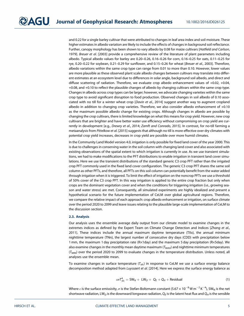
We first present the applied forcing of each of the experiments in terms of the mean change (EXP minus CTL)in the grid-scale surface albedo (α= SWU/SWD; Figures 1a–1f) and the irrigation amount (Figures 1g–1h) over

Figure 1. Contour map showing themean applied forcing (EXPminus CTL) over 2020–2099: (a–f) the grid-scale surface albedo (α = 100 × SWU/SWD; %) and (g–h) theirrigation amount (QIRR; mm yr�1). For experiments: ALB02 (Figure 1a), ALB04 (Figure 1b), ALB08 (Figure 1c), ALB10 (Figure 1d), IRRIG (Figures 1e and 1g), andIRRALB (Figures 1f and 1h). All maps are derived using the three-member ensemble mean of each configuration. Note that changes over the oceans have beenmasked. The red boxes in Figure 1a denote the four SREX regions presented in subsequent figures: Central North America (CNA), Central Europe (CEU), North Asia(NAS), and South Asia (SAS).



2020–2099. The grid-scale surface albedo increases with the scale of crop albedo enhancement over themajor agricultural regions in all experiments where it is applied (i.e., ALB02, ALB04, ALB08, ALB10, andIRRALB). Indeed, there is a slight decrease (~2–4%) in the grid-scale surface albedo in IRRIG (Figure 1e)coincident with regions where irrigation is applied (e.g., Figures 1g–1h). This is likely due to how the soilalbedo is calculated in the Community Land Model, where it is a function of the soil color and soilmoisture content [Oleson et al., 2013]. The irrigation amounts applied over 2020–2099 show that irrigationis triggered over Central North America, Argentina, the Sahel, Eurasia, India, and Southeast Australia. Themean global irrigation amount is 2430 km3 yr�1 (±143 km3 yr�1) for IRRIG and 2222 km3 yr�1 (±143 km3 yr�1)for IRRALB. In the context of the observed quantity applied today of 2664 km3 yr�1 [Sacks et al., 2009], theamounts of irrigation applied in our simulations are comparable to the present-day irrigation rates and fallwithin the range of observational uncertainty. However, the spatial extent is less than the present day spatialdistribution [e.g., Sacks et al., 2009] due to the constraint we impose in our simulations to limit irrigation towhere crops are the dominant vegetation cover. Therefore, it is possible that the mitigation potential of irri-gation is underestimated by not including all regions where irrigation is currently practiced or the potentialexpansion of irrigation to regions where crops are currently rainfed.

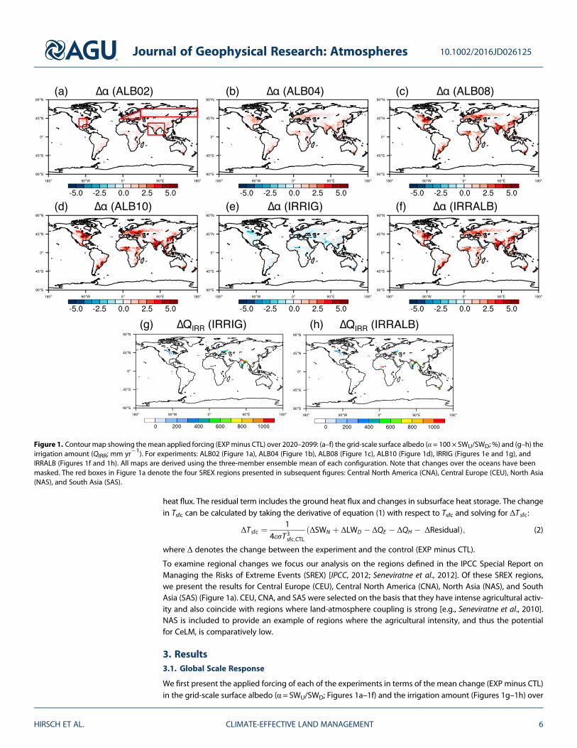
Although the forcing is similar between the ensemble members of a given experiment, estimates of thechange in the annual maximum daytime temperature (TXx) over 2020–2099 from individual simulations werenoisy (not shown). These were substantially improved when examining changes in TXx from the ensemblemean, particularly over regions where the forcing is greatest (Figure 2). More specifically, the magnitude ofthe crop albedo enhancement (Figures 2a–2d) is critical for obtaining a robust cooling response. For example,ALB02 (Figure 2a) tends to experience more warming than cooling; however, most TXx changes are within±0.3°C and generally not statistically significant. For ALB04 (Figure 2b), TXx decreases by ~1°C over NorthAmerica and between 0.5°C and 1°C over Eurasia. These regions expand in ALB08 (Figure 2c) and ALB10(Figure 2d) with a decrease in TXx of 1–2°C. While the application of crop albedo enhancement can bespatially constrained, the effects on climate are not entirely bounded to those regions, with some nonzerochanges occurring over regions where limited or no albedo changes were applied. For IRRIG (Figure 2e) thereis cooling of more than 2°C over North America, Eurasia, and India, but warming of ~1°C over SoutheastAsia and Southern China. This warming of TXx is symptomatic of changes in monsoon precipitation (see

Figure 2. Contour map showing the mean change (EXP minus CTL) in the annual maximum daytime temperature (TXx; °C) over 2020–2099. For experiments:(a) ALB02, (b) ALB04, (c) ALB08, (d) ALB10, (e) IRRIG, and (f) IRRALB. All maps are derived using the three-member ensemble mean of each configuration. Notethat changes over the oceans have been masked. Stippling indicates regions where the change is statistically significant at the 95% confidence level (determinedfrom a 1000 bootstrap sampling procedure with a two-sided test of the paired difference between two means).



Figures S1 to S4 in the supporting information). The cooling over North America, Eurasia, and India increasesand expands further in IRRALB (Figure 2f), where TXx decreases by more than 2°C. Therefore, IRRALB appearsto have the most robust cooling response of all the experiments.

3.2. Regional Scale Response

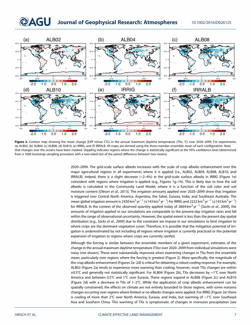
Between all the experiments, the regional differences are subtle and best illustrated by examining the regio-nal trend in the TXx anomaly relative to 1850–1870 as a function of the CO2 concentration (Figure 3). Wefocus on four different IPCC SREX regions: Central Europe (CEU), Central North America (CNA), North Asia(NAS), and South Asia (SAS) and examine changes across the land surface encompassed by each region.All panels in Figure 3 include the change in the global mean temperature anomaly (ΔTGM ; dashed lines)for each configuration. The change in ΔTGM between all experiments is negligible (i.e., dashed lines overlap),demonstrating that the changes in temperature induced by the CeLM schemes examined here do not sub-stantially change the global mean temperature but do affect temperature at regional scales. Figure 3 illus-trates the importance of the magnitude of the crop albedo enhancement, complementing the results ofFigures 2a–2d. In particular, for CEU (Figure 3a) ALB02 and ALB04 are barely distinguishable from the CTLensemble range, while ALB08 and ALB10 have comparable decreases in the TXx anomaly. Similarly for CNA

Figure 3. Regional temperature scaling with CO2 concentration (ppm) over 1850 to 2099 for four different SREX regions: (a)CEU, (b) CNA, (c) NAS, and (d) SAS. Solid lines correspond to the regional average annual maximum daytime temperature(TXx) anomaly, and dashed lines correspond to the global mean temperature anomaly, where all temperature anomaliesare relative to 1850–1870 and units are in °C. The black line in all panels denotes the three-member control ensemblemean with the grey-shaded regions corresponding to the ensemble range. The colored lines correspond to the three-member ensemble means of ALB02 (cyan), ALB04 (purple), ALB08 (orange), ALB10 (red), IRRIG (blue), and IRRALB (green).



(Figure 3b), larger increases in albedo are necessary to distinguish the cooling potential of crop albedoenhancement from the CTL ensemble range. For NAS and SAS (Figures 3c and 3d), all levels of crop albedoenhancement are barely distinguishable from the CTL ensemble range, although there is a subtle decreasein the TXx anomaly with increased crop albedo enhancement.

Comparing between the different CeLM schemes: crop albedo enhancement (ALB10), irrigation (IRRIG), andboth (IRRALB) illustrate that there are differences in the cooling potential of TXx. For CEU (Figure 3a), ALB10contributes a ~1°C decrease in the TXx anomaly over 2020–2099, IRRIG contributes a ~2°C decrease, and

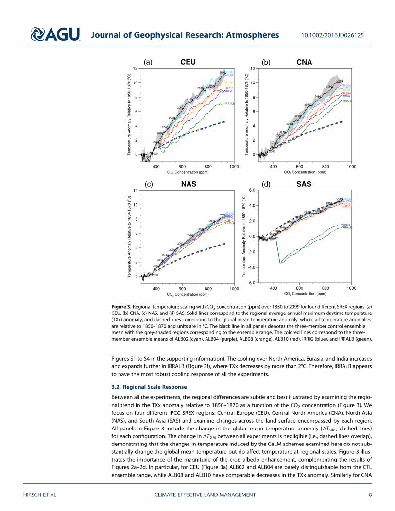
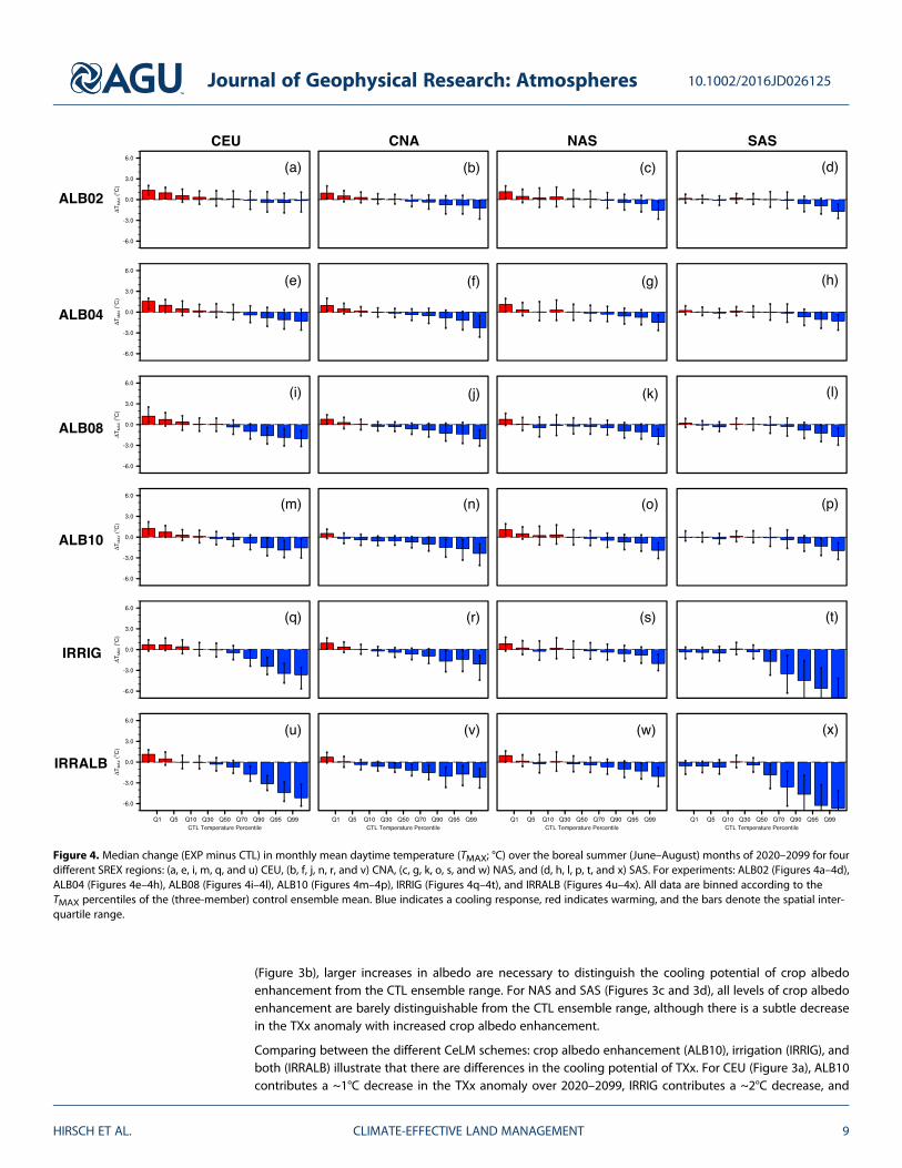
Figure 4. Median change (EXP minus CTL) in monthly mean daytime temperature (TMAX; °C) over the boreal summer (June–August) months of 2020–2099 for fourdifferent SREX regions: (a, e, i, m, q, and u) CEU, (b, f, j, n, r, and v) CNA, (c, g, k, o, s, and w) NAS, and (d, h, l, p, t, and x) SAS. For experiments: ALB02 (Figures 4a–4d),ALB04 (Figures 4e–4h), ALB08 (Figures 4i–4l), ALB10 (Figures 4m–4p), IRRIG (Figures 4q–4t), and IRRALB (Figures 4u–4x). All data are binned according to theTMAX percentiles of the (three-member) control ensemble mean. Blue indicates a cooling response, red indicates warming, and the bars denote the spatial inter-quartile range.



IRRALB contributes a ~3°C decrease in the TXx anomaly. Indeed, for IRRALB the trajectory of the TXx anomalyis below ΔTGM up until 2060. For CNA (Figure 3b) both ALB10 and IRRIG show comparable decreases in theTXx anomaly of ~1.5°C until 2070. The TXx anomaly for IRRALB also follows ΔTGM until 2060. For NAS(Figure 3c), the change in the TXx anomaly is limited, although decreases achieved in ALB10 are marginallygreater than IRRIG, and changes by ~�0.5°C for IRRALB. In contrast, for SAS (Figure 3d) the change in TXxfrom irrigation is considerable, with a decrease of the TXx anomaly of ~3°C for IRRIG and IRRALB. Figure 3demonstrates that the efficacy of CeLM is region dependent and that no scheme can maintain regionaltemperature extremes within the global mean temperature anomaly over the entire period 2020–2099.Therefore, CeLM cannot offset global warming. Finally, the application of both crop albedo enhancementand irrigation (IRRALB) generally achieves the largest decrease in the TXx anomaly across all regions shownhere, despite their respective different mechanisms for achieving cooling (see section 3.4).

3.3. Changes in Temperature Distribution

Given the changes in TXx shown in Figures 2 and 3, it is anticipated that the impact of CeLM is notconstrained to changing the upper tail of the temperature distribution. Using monthly mean daytime tem-peratures (TMAX) we examine the change (EXP minus CTL) in the daytime temperature distribution overthe summer months when CeLM is active in all experiments (Figure 4). Here all data are binned accordingto different percentiles with the bin edges at the 1st, 5th, 10th, 30th, 50th (median), 70th, 90th, 95th, and99th percentiles of the CTL ensemble mean. All data points (through space and time) within a region areranked to determine the median and interquartile range of the change for each bin. Again, we focus onthe same SREX regions as in Figure 3: CEU, CNA, NAS, and SAS (corresponding to the columns) and the dif-ferent experiments (corresponding to the rows). Generally, the cooling response in most experiments (parti-cularly in Figures 4i–4x) is greatest for the hot temperature extremes (i.e., Q90, Q95, and Q99) than themedian (i.e., Q50). For example, cooling over CEU for ALB10 (Figure 4m) increases in magnitude from�0.5°C at the median (Q50) to �2°C for the highest percentile (Q99); however, there is also a warmingresponse for the lowest percentile of +1.5°C (Q1). In fact this is generally true in most panels of Figure 4,except for those corresponding to SAS. In particular, for small levels of crop albedo enhancement (e.g.,ALB02 and ALB04; Figures 4a–4c and 4e–4g), the warming of the lower percentiles (Q1, Q5, and Q10) oftenoffsets any cooling achieved in the upper percentiles (Q90, Q95, and Q99). This is consistent with the resultsof Figures 3 where ALB02 and ALB04 were rarely distinguishable from the CTL ensemble range. This suggeststhat small levels of crop albedo enhancement are unlikely to achieve a robust cooling effect.

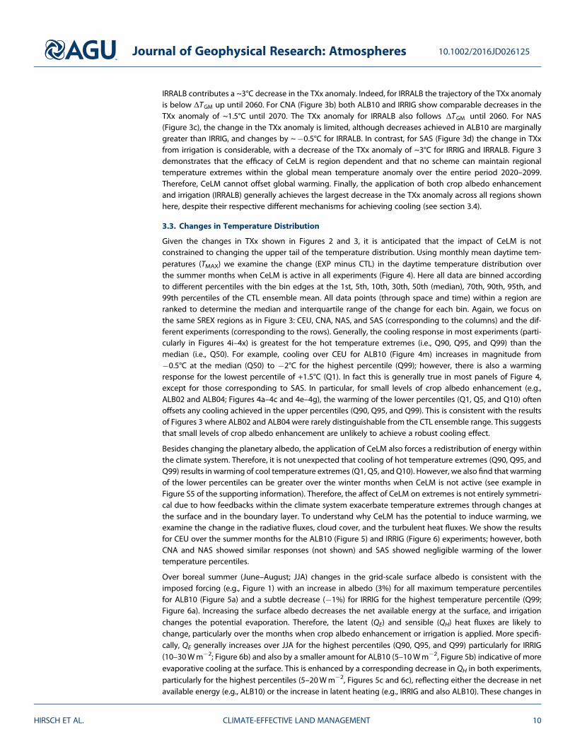
Besides changing the planetary albedo, the application of CeLM also forces a redistribution of energy withinthe climate system. Therefore, it is not unexpected that cooling of hot temperature extremes (Q90, Q95, andQ99) results in warming of cool temperature extremes (Q1, Q5, and Q10). However, we also find that warmingof the lower percentiles can be greater over the winter months when CeLM is not active (see example inFigure S5 of the supporting information). Therefore, the affect of CeLM on extremes is not entirely symmetri-cal due to how feedbacks within the climate system exacerbate temperature extremes through changes atthe surface and in the boundary layer. To understand why CeLM has the potential to induce warming, weexamine the change in the radiative fluxes, cloud cover, and the turbulent heat fluxes. We show the resultsfor CEU over the summer months for the ALB10 (Figure 5) and IRRIG (Figure 6) experiments; however, bothCNA and NAS showed similar responses (not shown) and SAS showed negligible warming of the lowertemperature percentiles.

Over boreal summer (June–August; JJA) changes in the grid-scale surface albedo is consistent with theimposed forcing (e.g., Figure 1) with an increase in albedo (3%) for all maximum temperature percentilesfor ALB10 (Figure 5a) and a subtle decrease (�1%) for IRRIG for the highest temperature percentile (Q99;Figure 6a). Increasing the surface albedo decreases the net available energy at the surface, and irrigationchanges the potential evaporation. Therefore, the latent (QE) and sensible (QH) heat fluxes are likely tochange, particularly over the months when crop albedo enhancement or irrigation is applied. More specifi-cally, QE generally increases over JJA for the highest percentiles (Q90, Q95, and Q99) particularly for IRRIG(10–30Wm�2; Figure 6b) and also by a smaller amount for ALB10 (5–10Wm�2, Figure 5b) indicative of moreevaporative cooling at the surface. This is enhanced by a corresponding decrease in QH in both experiments,particularly for the highest percentiles (5–20Wm�2, Figures 5c and 6c), reflecting either the decrease in netavailable energy (e.g., ALB10) or the increase in latent heating (e.g., IRRIG and also ALB10). These changes in



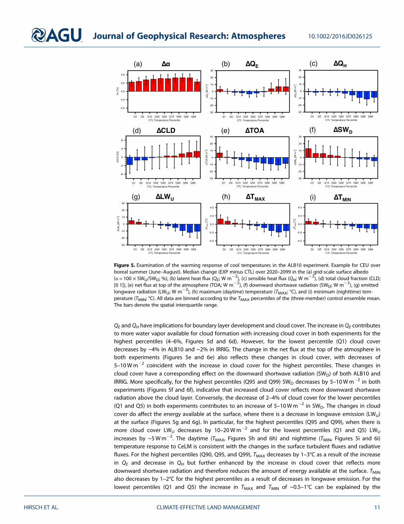
QE and QH have implications for boundary layer development and cloud cover. The increase in QE contributesto more water vapor available for cloud formation with increasing cloud cover in both experiments for thehighest percentiles (4–6%, Figures 5d and 6d). However, for the lowest percentile (Q1) cloud coverdecreases by ~4% in ALB10 and ~2% in IRRIG. The change in the net flux at the top of the atmosphere inboth experiments (Figures 5e and 6e) also reflects these changes in cloud cover, with decreases of5–10Wm�2 coincident with the increase in cloud cover for the highest percentiles. These changes incloud cover have a corresponding effect on the downward shortwave radiation (SWD) of both ALB10 andIRRIG. More specifically, for the highest percentiles (Q95 and Q99) SWD decreases by 5–10Wm�2 in bothexperiments (Figures 5f and 6f), indicative that increased cloud cover reflects more downward shortwaveradiation above the cloud layer. Conversely, the decrease of 2–4% of cloud cover for the lower percentiles(Q1 and Q5) in both experiments contributes to an increase of 5–10Wm�2 in SWD. The changes in cloudcover do affect the energy available at the surface, where there is a decrease in longwave emission (LWU)at the surface (Figures 5g and 6g). In particular, for the highest percentiles (Q95 and Q99), when there ismore cloud cover LWU decreases by 10–20Wm�2 and for the lowest percentiles (Q1 and Q5) LWU

increases by ~5Wm�2. The daytime (TMAX, Figures 5h and 6h) and nighttime (TMIN, Figures 5i and 6i)temperature response to CeLM is consistent with the changes in the surface turbulent fluxes and radiativefluxes. For the highest percentiles (Q90, Q95, and Q99), TMAX decreases by 1–3°C as a result of the increasein QE and decrease in QH but further enhanced by the increase in cloud cover that reflects moredownward shortwave radiation and therefore reduces the amount of energy available at the surface. TMIN

also decreases by 1–2°C for the highest percentiles as a result of decreases in longwave emission. For thelowest percentiles (Q1 and Q5) the increase in TMAX and TMIN of ~0.5–1°C can be explained by the

Figure 5. Examination of the warming response of cool temperatures in the ALB10 experiment. Example for CEU overboreal summer (June–August). Median change (EXP minus CTL) over 2020–2099 in the (a) grid-scale surface albedo(α = 100 × SWU/SWD; %), (b) latent heat flux (QE; W m�2), (c) sensible heat flux (QH; W m�2), (d) total cloud fraction (CLD;[0 1]), (e) net flux at top of the atmosphere (TOA; W m�2), (f) downward shortwave radiation (SWD; W m�2), (g) emittedlongwave radiation (LWU; W m�2), (h) maximum (daytime) temperature (TMAX; °C), and (i) minimum (nighttime) tem-perature (TMIN; °C). All data are binned according to the TMAX percentiles of the (three-member) control ensemble mean.The bars denote the spatial interquartile range.



decrease in cloud cover which enables more shortwave radiation to reach the surface. Therefore, changes inthe temperature distribution reflect changes in available energy that are at first an immediate response todirect changes in the surface energy balance from CeLM that then evolve to influence cloud cover.

We note here that the increase in cloud cover over the summer months does not dissipate at the end of thegrowing season when CeLM ceases. Rather, the increased cloud cover persists over the winter months. Overthe winter months the climate system does not fully return to an unperturbed state due the changes in thehydrological cycle that are initiated over the period when CeLM is active. The hydrological response takeslonger relative to the instantaneous changes in available energy through albedo change upon the cessationof CeLM. Increased cloud cover during winter thus leads to additional warming through increased LWD

(Figure S5).

We also checked the change in minimum temperature (TMIN) and the annual minimum nighttime tempera-ture (TNn; Figures S6 and S7 in the supporting information). Generally, TMIN decreases between �0.2°C and�1°C over the same regions of North America, Eurasia, and India where TXx (and TMAX; Figure S8) decreases.However, TMIN increases of more than +0.5°C are found in ALB02 and also in IRRIG over regions where irriga-tion was not enabled. Similar spatial patterns are found with TNn, although the decreases and increases aregenerally larger in magnitude than those for TMIN. The decrease in TMAX is generally larger than the decreasein TMIN and therefore there is a narrowing of the diurnal temperature range of ~1°C over North America,Europe, and India for the ALB10, IRRIG, and IRRALB experiments (Figure S9). Over Southeast Asia in IRRIGand IRRALB the diurnal range increases by more than 1°C where changes in monsoon precipitation wereevident (Figure S2 to S4).

3.4. Mechanisms for Regional Differences

Figure 3 demonstrated that the CeLM schemes lead to different magnitudes of TXx cooling where either irri-gation (e.g., CEU, Figure 3a) or crop albedo enhancement (e.g., NAS, Figure 3c) was more effective at reducingTXx, or both were comparable for part of the period 2020–2099 (e.g., CNA, Figure 3b). A similar pattern

Figure 6. As is Figure 5 but for the IRRIG experiment.



emerges when comparing the changes in the TMAX distribution between ALB10 and IRRIG (Figures 4m–4t).To understand why these regional differences exist, we consider how each CeLM scheme, crop albedoenhancement, and irrigation changes the surface energy balance. Crop albedo enhancement achievescooling initially by decreasing the amount of energy available at the surface (e.g., Figure 5a), contributingto a decrease in QH (Figure 5c) and partly in QE (Figure 5b). However, changes in the partitioning betweenQH and QE also occur and lead to an increase QE, particularly for the higher percentiles (Q90, Q95, and Q99,Figure 5b). This in turn leads to enhanced water vapor in the lower atmosphere that triggers an increasein cloud cover (Figure 5d). The increase in cloud cover further limits downward shortwave radiation(Figure 5f), thus acting as a positive feedback for surface cooling. Irrigation achieves cooling by increasingthe evaporative fraction (Figure 6b). This change in the partitioning between QH and QE also triggers anincrease in cloud cover (Figure 6d) and associated decrease in downward shortwave radiation (Figure 6f),again leading to further cooling. Therefore, crop albedo enhancement triggers the change in the surfaceenergy balance by altering the net energy available at the surface through albedo and irrigation changesthe partitioning between QE and QH through increased soil moisture. To determine which flux triggers thelargest change (EXP minus CTL) in surface temperature, we use the surface energy balance decompositionapproach explained in section 2.3.

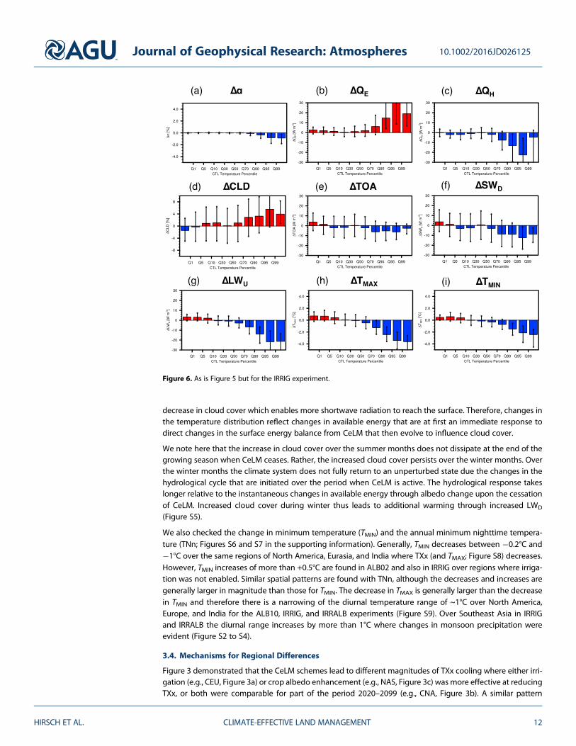
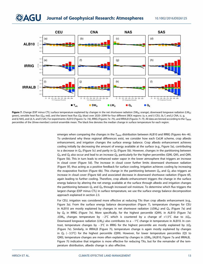
For CEU, irrigation was considered more effective at reducing TXx than crop albedo enhancement (e.g.,Figure 3a). From the surface energy balance decomposition (Figure 7), temperature changes for CEUin ALB10 are mostly explained by changes in net shortwave radiation (ΔSWN) and QH (Figure 7a) andby QE in IRRIG (Figure 7e). More specifically, for the highest percentile (Q99), in ALB10 (Figure 7a)ΔSWN changes temperature by �2°C which is countered by a change of +1.5°C due to ΔQH.Downward longwave radiation (LWD) also contributes to a �1°C change in temperature in ALB10. In con-trast, temperature changes by �3°C in IRRIG for the highest percentile are mostly explained by ΔQE

(Figure 7e). Similarly, in IRRALB (Figure 7i), temperature change is again mostly explained by changesin QE (�3.5°C) for the highest percentile (Q99). However, for lower temperature percentiles (Q5 toQ90), temperature changes are more often explained by changes in ΔSWN (ALB10, Figure 7a and IRRALB,Figure 7i) indicative that irrigation is more effective for reducing TXx, but for the remainder of the tem-perature distribution, albedo change is also effective.

Figure 7. Change (EXP minus CTL) surface temperature explained by changes in the net shortwave radiation (SWN; orange), downward longwave radiation (LWD;green), sensible heat flux (QH; red), and the latent heat flux (QE; blue) over 2020–2099 for four different SREX regions: (a, e, and i) CEU, (b, f, and j) CNA, (c, g,and k) NAS, and (d, h, and l) SAS. For experiments: ALB10 (Figures 7a–7d), IRRIG (Figures 7e–7h), and IRRALB (Figures 7i–7l). All data are binned according to the TMAXpercentiles of the (three-member) control ensemble mean. The black line denotes the median change in surface temperature for each region.



For CNA both crop albedo enhance-ment and irrigation are comparablein their effect on reducing TXx over2020–2070 (e.g., Figure 3b). For thehighest percentile (Q99), tempera-ture changes of �4°C in both ALB10(Figure 7b) and IRRIG (Figure 7f) aredue to ΔQE . However, ΔQH contri-butes a +4°C change in temperaturein ALB10 and +3.5°C in IRRIG. ForIRRALB (Figure 7j), temperaturechange of the highest percentileis also mostly attributed to ΔQH.Consequently, the actual change intemperature over CNA for the high-est percentile is similar betweenALB10, IRRIG, and IRRALB (�2.5°C)suggesting that of the CeLM schemes

examined here, none has a substantial advantage above the others. As in CEU, CNA temperature changes ofthe lower percentiles (Q5 to Q90) tend to be explained by ΔSWN (ALB10, Figure 7b and IRRALB, Figure 7j).

For NAS crop albedo, enhancement was often more effective at reducing TXx than irrigation (e.g., Figure 3c)in part because irrigation was rarely triggered over this region (e.g., Figure 1g). For ALB10 (Figure 7c) andIRRALB (Figure 7k) temperature change over NAS is mostly associated with ΔSWN and ΔLWD particularlyfor the tails of the temperature distribution (Q1, Q5, Q95, and Q99). For the highest percentile (Q99), ΔQH

also contributes to +1°C in all experiments over NAS (Figures 7c, 7g, and 7k). Therefore, over NAS, changesin available energy are the critical driver of temperature change and these were largely determined byalbedo change.

For SAS, irrigation has a substantial effect on TXx (e.g., Figure 3d) that is associated with the higher ratesapplied over the region (e.g., Figure 1g). In ALB10 (Figure 7d), IRRIG (Figure 7h) and IRRALB (Figure 7l),temperature change of the highest percentile (Q99) is dominated by changes in the partitioning betweenQE and QH. The actual temperature change in IRRIG and IRRALB is substantially larger than ALB10 (�6°Ccompared to �2°C) reflecting the larger changes in QE and QH.

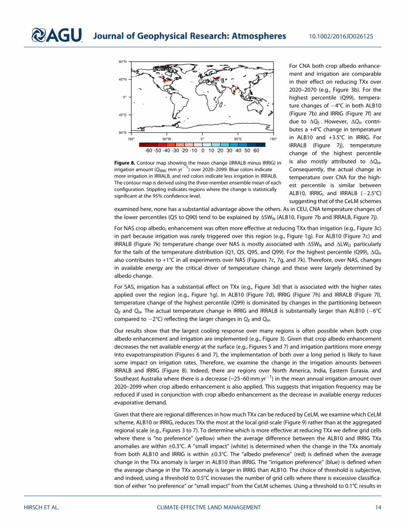
Our results show that the largest cooling response over many regions is often possible when both cropalbedo enhancement and irrigation are implemented (e.g., Figure 3). Given that crop albedo enhancementdecreases the net available energy at the surface (e.g., Figures 5 and 7) and irrigation partitions more energyinto evapotranspiration (Figures 6 and 7), the implementation of both over a long period is likely to havesome impact on irrigation rates. Therefore, we examine the change in the irrigation amounts betweenIRRALB and IRRIG (Figure 8). Indeed, there are regions over North America, India, Eastern Eurasia, andSoutheast Australia where there is a decrease (~25–60mmyr�1) in the mean annual irrigation amount over2020–2099 when crop albedo enhancement is also applied. This suggests that irrigation frequency may bereduced if used in conjunction with crop albedo enhancement as the decrease in available energy reducesevaporative demand.

Given that there are regional differences in howmuch TXx can be reduced by CeLM, we examine which CeLMscheme, ALB10 or IRRIG, reduces TXx the most at the local grid-scale (Figure 9) rather than at the aggregatedregional scale (e.g., Figures 3 to 7). To determine which is more effective at reducing TXx we define grid cellswhere there is “no preference” (yellow) when the average difference between the ALB10 and IRRIG TXxanomalies are within ±0.3°C. A “small impact” (white) is determined when the change in the TXx anomalyfrom both ALB10 and IRRIG is within ±0.3°C. The “albedo preference” (red) is defined when the averagechange in the TXx anomaly is larger in ALB10 than IRRIG. The “irrigation preference” (blue) is defined whenthe average change in the TXx anomaly is larger in IRRIG than ALB10. The choice of threshold is subjective,and indeed, using a threshold to 0.5°C increases the number of grid cells where there is excessive classifica-tion of either “no preference” or “small impact” from the CeLM schemes. Using a threshold to 0.1°C results in

Figure 8. Contour map showing the mean change (IRRALB minus IRRIG) inirrigation amount (QIRR; mm yr�1) over 2020–2099. Blue colors indicatemore irrigation in IRRALB, and red colors indicate less irrigation in IRRALB.The contour map is derived using the three-member ensemble mean of eachconfiguration. Stippling indicates regions where the change is statisticallysignificant at the 95% confidence level.



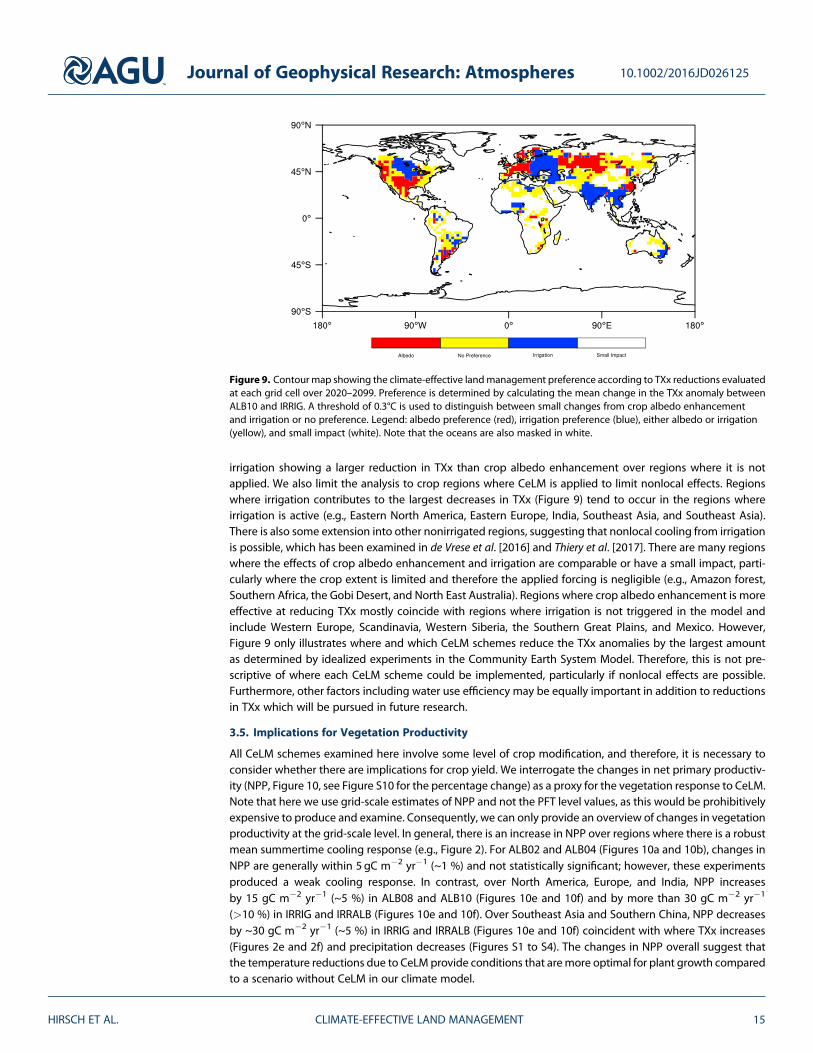
irrigation showing a larger reduction in TXx than crop albedo enhancement over regions where it is notapplied. We also limit the analysis to crop regions where CeLM is applied to limit nonlocal effects. Regionswhere irrigation contributes to the largest decreases in TXx (Figure 9) tend to occur in the regions whereirrigation is active (e.g., Eastern North America, Eastern Europe, India, Southeast Asia, and Southeast Asia).There is also some extension into other nonirrigated regions, suggesting that nonlocal cooling from irrigationis possible, which has been examined in de Vrese et al. [2016] and Thiery et al. [2017]. There are many regionswhere the effects of crop albedo enhancement and irrigation are comparable or have a small impact, parti-cularly where the crop extent is limited and therefore the applied forcing is negligible (e.g., Amazon forest,Southern Africa, the Gobi Desert, and North East Australia). Regions where crop albedo enhancement is moreeffective at reducing TXx mostly coincide with regions where irrigation is not triggered in the model andinclude Western Europe, Scandinavia, Western Siberia, the Southern Great Plains, and Mexico. However,Figure 9 only illustrates where and which CeLM schemes reduce the TXx anomalies by the largest amountas determined by idealized experiments in the Community Earth System Model. Therefore, this is not pre-scriptive of where each CeLM scheme could be implemented, particularly if nonlocal effects are possible.Furthermore, other factors including water use efficiency may be equally important in addition to reductionsin TXx which will be pursued in future research.

3.5. Implications for Vegetation Productivity

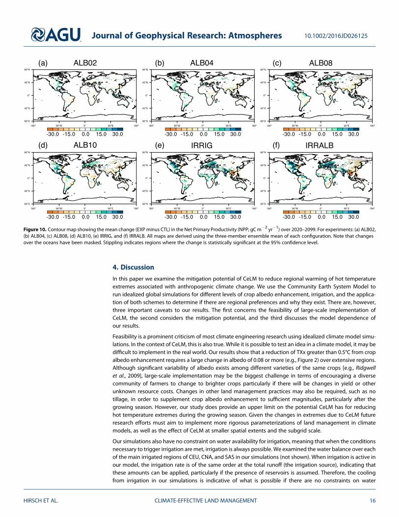
All CeLM schemes examined here involve some level of crop modification, and therefore, it is necessary toconsider whether there are implications for crop yield. We interrogate the changes in net primary productiv-ity (NPP, Figure 10, see Figure S10 for the percentage change) as a proxy for the vegetation response to CeLM.Note that here we use grid-scale estimates of NPP and not the PFT level values, as this would be prohibitivelyexpensive to produce and examine. Consequently, we can only provide an overview of changes in vegetationproductivity at the grid-scale level. In general, there is an increase in NPP over regions where there is a robustmean summertime cooling response (e.g., Figure 2). For ALB02 and ALB04 (Figures 10a and 10b), changes inNPP are generally within 5 gC m�2 yr�1 (~1 %) and not statistically significant; however, these experimentsproduced a weak cooling response. In contrast, over North America, Europe, and India, NPP increasesby 15 gC m�2 yr�1 (~5 %) in ALB08 and ALB10 (Figures 10e and 10f) and by more than 30 gC m�2 yr�1

(>10 %) in IRRIG and IRRALB (Figures 10e and 10f). Over Southeast Asia and Southern China, NPP decreasesby ~30 gC m�2 yr�1 (~5 %) in IRRIG and IRRALB (Figures 10e and 10f) coincident with where TXx increases(Figures 2e and 2f) and precipitation decreases (Figures S1 to S4). The changes in NPP overall suggest thatthe temperature reductions due to CeLM provide conditions that aremore optimal for plant growth comparedto a scenario without CeLM in our climate model.

Figure 9. Contour map showing the climate-effective landmanagement preference according to TXx reductions evaluatedat each grid cell over 2020–2099. Preference is determined by calculating the mean change in the TXx anomaly betweenALB10 and IRRIG. A threshold of 0.3°C is used to distinguish between small changes from crop albedo enhancementand irrigation or no preference. Legend: albedo preference (red), irrigation preference (blue), either albedo or irrigation(yellow), and small impact (white). Note that the oceans are also masked in white.



4. Discussion

In this paper we examine the mitigation potential of CeLM to reduce regional warming of hot temperatureextremes associated with anthropogenic climate change. We use the Community Earth System Model torun idealized global simulations for different levels of crop albedo enhancement, irrigation, and the applica-tion of both schemes to determine if there are regional preferences and why they exist. There are, however,three important caveats to our results. The first concerns the feasibility of large-scale implementation ofCeLM, the second considers the mitigation potential, and the third discusses the model dependence ofour results.

Feasibility is a prominent criticism of most climate engineering research using idealized climate model simu-lations. In the context of CeLM, this is also true. While it is possible to test an idea in a climate model, it may bedifficult to implement in the real world. Our results show that a reduction of TXx greater than 0.5°C from cropalbedo enhancement requires a large change in albedo of 0.08 or more (e.g., Figure 2) over extensive regions.Although significant variability of albedo exists among different varieties of the same crops [e.g., Ridgwellet al., 2009], large-scale implementation may be the biggest challenge in terms of encouraging a diversecommunity of farmers to change to brighter crops particularly if there will be changes in yield or otherunknown resource costs. Changes in other land management practices may also be required, such as notillage, in order to supplement crop albedo enhancement to sufficient magnitudes, particularly after thegrowing season. However, our study does provide an upper limit on the potential CeLM has for reducinghot temperature extremes during the growing season. Given the changes in extremes due to CeLM futureresearch efforts must aim to implement more rigorous parameterizations of land management in climatemodels, as well as the effect of CeLM at smaller spatial extents and the subgrid scale.

Our simulations also have no constraint on water availability for irrigation, meaning that when the conditionsnecessary to trigger irrigation aremet, irrigation is always possible. We examined the water balance over eachof the main irrigated regions of CEU, CNA, and SAS in our simulations (not shown). When irrigation is active inour model, the irrigation rate is of the same order at the total runoff (the irrigation source), indicating thatthese amounts can be applied, particularly if the presence of reservoirs is assumed. Therefore, the coolingfrom irrigation in our simulations is indicative of what is possible if there are no constraints on water

Figure 10. Contour map showing themean change (EXPminus CTL) in the Net Primary Productivity (NPP; gCm�2 yr�1) over 2020–2099. For experiments: (a) ALB02,(b) ALB04, (c) ALB08, (d) ALB10, (e) IRRIG, and (f) IRRALB. All maps are derived using the three-member ensemble mean of each configuration. Note that changesover the oceans have been masked. Stippling indicates regions where the change is statistically significant at the 95% confidence level.



resources. However, in the real world water limitations associated with droughts, like the millennium droughtexperienced in Australia [van Dijk et al., 2013], impose limits on the ability to irrigate sustainably. Furthermore,Feng et al. [2016] find that the revegetation program of the Loess Plateau of China is actually contributing toan additional constraint on water availability due to increases in evapotranspiration reducing runoff intoreservoirs. Therefore, water constraints on irrigation are likely to be exacerbated with climate change, wherefurther changes in the hydrological cycle could affect the future distribution of water resources available forirrigation [IPCC, 2013]. Future research is planned to implement such constraints on irrigation to examine thelong-term potential of irrigation in a 2°C (or more) world.

Our results focus on themitigation potential of CeLM on hot temperature extremes and not cold temperatureextremes or precipitation. However, the identification of a positive feedback on cloud development that con-tributes to temperature warming during the winter months when CeLM is temporarily suspended requiresconfirmation in other ESMs. In particular, the benefits of CeLM are perhaps negligible for regions wherethe summertime cooling from CeLM is offset by warming of comparable magnitudes in winter. Changes intemperature due to cloud cover over months when CeLM is not active may be resolved if no till is employedafter the growing season to minimize the change in albedo between seasons; however, this hypothesisrequires further investigation. Termination effects in other climate engineering schemes have been identi-fied, with the most severe consequences associated with stratospheric aerosol injection [e.g., Aswathyet al., 2015; Curry et al., 2014; Crook et al., 2015]. However, to our knowledge our study is the first to considerthe impacts of temporary cessation of CeLM. Before any real-world application of CeLM can be considered,more research is required to quantify the risk of negative impacts from temporary suspension or completecessation of CeLM.

Further limitations on the mitigation potential of CeLM pertain to the experimental design where wecompare all experiments to a control where there is no irrigation, despite the fact that irrigation alreadyexists now. Therefore, the mitigation potential from irrigation is perhaps already realized in the past andcan only be increased by expanding to regions where irrigation is currently not employed. However, thisexpansion will depend critically on the sustainable use of future water resources. Another unknown con-sequence of CeLM is whether there will be changes in crop yield. Although we find increases in NPPsuggesting more productive vegetation, we cannot state if this means yields will also increase. The effectof stratospheric aerosol injection on vegetation has been examined in Xia et al. [2016] and Glienke et al.[2015] who find an increase in NPP due to increases in diffuse radiation and cooling associated with stra-tospheric aerosol injection. However, in the context of CeLM, not enough is known on whether brightercrops yield bigger harvests.

Finally, we cannot exclude the model dependence of our results. Previous studies examining the potential ofcrop albedo enhancement using the same model have found similar cooling responses to those reportedhere [e.g., Lobell et al., 2006; Wilhelm et al., 2015]. We find that the potential of land-based schemes relativeto climate engineering schemes has been understated in previous research due to the focus on climatemeans rather than extremes. Furthermore, we are not the first to examine the impact of climate engineeringon extremes or identify an asymmetric response of temperature extremes to climate engineering [e.g., Curryet al., 2014; Davin et al., 2014; Aswathy et al., 2015; Wilhelm et al., 2015]. In particular, analysis of multimodelsimulations by Aswathy et al. [2015] report that both stratospheric aerosol injection and marine cloud bright-ening are able to decrease hot temperature extremes more thanmean temperature, but provide limited miti-gation potential for cold temperature extremes. This was also found in Curry et al. [2014], who examine theimpact of solar reduction geoengineering on climate extremes in the GeoMIP G1 multimodel experiment,where warming of cold temperature extremes could not be avoided. This increase in minimum temperaturesassociated with stratospheric aerosol injection, marine cloud brightening, and solar reduction geoengineer-ing in other studies is likely associated with the fact that these schemes are “active” during the daytime byreducing shortwave radiation and not reducing GHG concentrations. Similarly, in our experiments, we foundsome regional decrease of cool temperature extremes, particularly for low levels of crop albedo enhance-ment (e.g., Figures 4 and S5). Given that our single-model experiment finds similar warming of cold tempera-ture extremes as multimodel experiments [e.g., Curry et al., 2014; Aswathy et al., 2015] it is perhaps anindication that most climate engineering is generally targeted at reducing hot extremes and not resolvingall the challenges associated with future anthropogenic climate change. Therefore, although we only use asingle model, we do find similarities between our results and those of previous studies. Resolving model



dependence can perhaps only be achieved by running coordinated CeLM experiments with several ESMs,which could involve the GeoMIP testbed [Kravitz et al., 2015].

5. Conclusions

Using idealized global simulations in an ESM, we have examined the potential of climate-effective land man-agement (CeLM), consisting of crop albedo enhancement and irrigation, to reduce regional warming of hotextremes associated with future anthropogenic climate change. We note that the approach applied here isdone globally while in reality the spatial extent may be less and therefore our results present the upper limit.We find that the considered CeLM implementations tend to be more effective at reducing hot temperatureextremes by more than 2°C, while the effect onmean or cold temperature extremes is much less. We also findthat implementing both irrigation and crop albedo enhancement is the most effective CeLM scheme that isexamined here, which also has the potential to reduce water use from irrigation through decreases inevaporative demand. To our knowledge we are the first to demonstrate this potential. Furthermore, regionaldifferences between irrigation and crop albedo enhancement were identified using a surface energy balancedecomposition method. The regional differences were linked to how they respectively change the surfaceenergy balance through changes in available energy and partitioning between QE and QH.

We find that a large albedo perturbation in our ESM is required to obtain a robust cooling response from cropalbedo enhancement. This may present challenges on the feasibility of real-world implementation; however,our results are valid for globally applied scenarios. Other climate engineering schemes are known to have asignificant termination effect. We find that over the winter months when CeLM is temporarily suspended,warming is possible due to persistent cloud cover that develops during the months when CeLM is active.Whether this is unique to the Community Earth System Model can only be confirmed by running similarexperiments in other ESMs. Finally, the mitigation potential of CeLM is often underappreciated in the litera-ture on idealized ESM experiments of climate engineering. However, our results demonstrate that perhapsthis is due to the historical focus on examining how climate engineering will affect mean climate, whereCeLM has limited influence, rather than the extremes where CeLM can have a substantial impact.

ReferencesAswathy, V. N., O. Boucher, M. Quaas, U. Niemeier, H. Muri, and J. Quaas (2015), Climate extremes in multi-model simulations of

stratospheric aerosol and marine cloud brightening climate engineering, Atmos. Chem. Phys., 15, 9593–9610, doi:10.5194/acp-15-9593-2015.

Breuer, L., K. Eckhardt, and H. G. Frede (2003), Plant parameter values for models in temperate climates, Ecol. Modell., 169, 237–293,doi:10.1016/S0304-3800(03)00274-6.

Caldeira, K., and G. Bala (2016), Reflecting on 50 years of geoengineering research, Earths Future, 4, 1–19, doi:10.1002/2016EF000454.Cao, L., L. Duan, G. Bala, and K. Caldeira (2016), Simulated long-term climate response to idealized solar geoengineering, Geophys. Res. Lett.,

43, 2209–2217, doi:10.1002/2016GL068079.Crook, J. A., L. S. Jackson, S. M. Osprey, and P. M. Forster (2015), A comparison of temperature and precipitation responses to different Earth

radiation management geoengineering schemes, J. Geophys. Res. Atmos., 120, 9352–9373, doi:10.1002/2015JD023269.Crook, J. A., L. S. Jackson, and P. M. Forster (2016), Can increasing albedo of existing ship wakes reduce climate change?, J. Geophys. Res.

Atmos., 121, 1545–1558, doi:10.1002/2015JD024201.Crutzen, P. J. (2006), Albedo enhancement by stratospheric sulfur injections: A contribution to resolve a policy dilemma?, Clim. Change, 77,

211–220, doi:10.1007/s10584-006-9101-y.Curry, C. L., et al. (2014), A multi-model examination of climate extremes in an idealized geoengineering experiment, J. Geophys. Res. Atmos.,

119, 3900–3923, doi:10.1002/2013JD020648.Davin, E. L., S. I. Seneviratne, P. Ciais, A. Olioso, and T. Wang (2014), Preferential cooling of hot extremes from cropland albedo management,

Proc. Natl. Acad. Sci. U.S.A., 111(27), 9757–9761, doi:10.1073/pnas.1317323111.de Vrese, P., S. Hagemann, and M. Claussen (2016), Asian irrigation, African rain: Remote impacts of irrigation, Geophys. Res. Lett., 43,

3737–3745, doi:10.1002/2016GL068146.Doughty, C. E., C. B. Field, and A. M. S. McMillan (2011), Can crop albedo be increased through the modification of leaf trichomes, and could

this cool regional climate?, Clim. Change, 104, 379–387, doi:10.1007/s10584-010-9936-0.Drewry, D. T., P. Kumar, and S. P. Long (2014), Simultaneous improvement in productivity, water use, and albedo through crop structural

modification, Global Change Biol., 20, 1955–1967, doi:10.1111/gcb.12567.Febrero, A., S. Fernandez, J. L. Molina-Cano, and J. L. Araus (1998), Yield, carbon isotope discrimination, canopy reflectance and cuticular

conductance of barley isolines of differing glaucousness, J. Exp. Bot., 49, 1575–1581, doi:10.1093/jxb/49.326.1575.Feng, X., et al. (2016), Revegetation in China’s Loess Plateau is approaching sustainable water resource limits, Nat. Clim. Change, 6,

1019–1022, doi:10.1038/nclimate3092.Fischer, E. M., U. Beyerle, and R. Knutti (2013), Robust spatially aggregated projections of climate extremes, Nat. Clim. Change, 3(12),

1033–1038, doi:10.1038/nclimate2051.Gabriel, C. J., A. Robock, L. Xia, B. Zambri, and B. Kravitz (2017), The G4Foam experiment: Global climate impacts of regional ocean albedo

modification, Atmos. Chem. Phys., 17, 595–613, doi:10.5194/acp-17-595-2017.



AcknowledgmentsWe thank National Center forAtmospheric Research (NCAR) for thedevelopment and access to theCommunity Earth System Model. Wegreatly thank the ETH Euler cluster forsupport with the computing resourcesof all climate model simulations. Theauthors would like to thank UrsBeyerle for providing the controlensemble simulations that were usedas initial conditions of all idealizedexperiments. All authors acknowledgethe European Research Council (ERC)“DROUGHT-HEAT” project funded bythe European Community’s SeventhFramework Programme (grant agree-ment FP7-IDEAS-ERC-617518). Allmaterials that have contributed to thereported results are available uponrequest, including 10 TB of model out-put. All requests for data and analysisscripts should be directed to the corre-sponding authors A.L. Hirsch ([email protected]) and S.I. Seneviratne([email protected]).

http://doi.org/10.5194/acp-15-9593-2015

http://doi.org/10.5194/acp-15-9593-2015

http://doi.org/10.1016/S0304-3800(03)00274-6

http://doi.org/10.1002/2016EF000454

http://doi.org/10.1002/2016GL068079

http://doi.org/10.1002/2015JD023269

http://doi.org/10.1002/2015JD024201

http://doi.org/10.1007/s10584-006-9101-y

http://doi.org/10.1002/2013JD020648

http://doi.org/10.1073/pnas.1317323111

http://doi.org/10.1002/2016GL068146

http://doi.org/10.1007/s10584-010-9936-0

http://doi.org/10.1111/gcb.12567

http://doi.org/10.1093/jxb/49.326.1575

http://doi.org/10.1038/nclimate3092


http://doi.org/10.5194/acp-17-595-2017




Gent, P. R., et al. (2011), The community climate system model version 4, J. Clim., 24, 4973–4991, doi:10.1175/2011JCLI4083.1.Glienke, S., P. J. Irvine, and M. G. Lawrence (2015), The impact of geoengineering on vegetation in experiment G1 of the GeoMIP, J. Geophys.

Res. Atmos., 120, 10,196–10,213, doi:10.1002/2015JD024202.Grant, R. H., G. M. Heisler, W. Gao, and M. Jenks (2003), Ultraviolet leaf reflectance of common urban trees and the prediction of reflectance

from leaf characteristics, Agric. For. Meteorol., 120, 127–139, doi:10.1016/j.ag1formet.2003.08.025.Hatfield, J. L., and R. E. Carlson (1979), Light quality distributions and spectral albedo of three maize canopies, Agric. Meteorol., 20, 215–226,

doi:10.1016/0002-1571(79)90022-0.Hurrell, J. W., et al. (2013), The community earth system model: A framework for collaborative research, Bull. Am. Meteorol. Soc., 94(9),

1339–1360, doi:10.1175/BAMS-D-12-00121.1.Hurtt, G. C., S. Frolking, M. G. Fearon, B. Moore, E. Sheviliakova, S. Malyshev, S. W. Pacala, and R. A. Houghton (2006), The underpinnings of

land-use history: Three centuries of global gridded land-use transitions, wood-harvest activity, and resulting secondary lands,Global Change Biol., 12, 1208–1229, doi:10.1111/j.1365-2486.2006.01150.x.

Intergovernmental Panel on Climate Change (IPCC) (2012), Managing the Risks of Extreme Events and Disasters to Advance ClimateChange Adaptation. A Special Report of Working Groups I and II of the Intergovernmental Panel on Climate Change, edited by C. B. Field et al.,582 pp., Cambridge Univ. Press, Cambridge, U. K., and New York.

Intergovernmental Panel on Climate Change (IPCC) (2013), Climate Change 2013: The Physical Science Basis. Contribution of Working Group I tothe Fifth Assessment Report of the Intergovernmental Panel on Climate Change, edited by T. F. Stocker et al., 1535 pp., Cambridge Univ.Press, Cambridge, U. K., and New York.

Irvine, P. J., A. Ridgwell, and D. J. Lunt (2010), Assessing the regional disparities in geoengineering impacts, Geophys. Res. Lett., 37, L18702,doi:10.1029/2010GL044447.

Irvine, P. J., A. Ridgwell, and D. J. Lunt (2011), Climatic effects of surface albedo geoengineering, J. Geophys. Res., 116, D24112, doi:10.1029/2011JD016281.

Irvine, P. J., B. Kravitz, M. G. Lawrence, and H. Muri (2016), An overview of the Earth system science of solar geoengineering, WIREs Clim.Change, 1–19, doi:10.1002/wcc.423.

Jones, A., J. Haywood, and O. Boucher (2009), Climate impacts of geoengineering marine stratocumulus clouds, J. Geophys. Res., 114, D10106,doi:10.1029/2008JD011450.

Jones, A., J. Haywood, O. Boucher, B. Kravitz, and A. Robock (2010), Geoengineering by stratospheric SO2 injection: Results from the MetOffice HadGEM2 climate model and comparison with the Goddard Institute for Space Studies ModelE, Atmos. Chem. Phys., 10, 5999–6006,doi:10.5194/acp-10-5999-2010.

Jones, A., et al. (2013), The impact of abrupt suspension of solar radiation management (termination effect) in experiment G2 of theGeoengineering Model Intercomparison Project (GeoMIP), J. Geophys. Res. Atmos., 118, 9743–9752, doi:10.1002/jgrd.50762.

Keith, D. (2000), Geoengineering the climate: History and prospect, Annu. Rev. Energy Environ., 25, 245–284.Keith, D. W., and P. J. Irvine (2016), Solar geoengineering could substantially reduce climate risks—A research hypothesis for the next decade,

Earths Future, 1–14, doi:10.1002/2016EF000465.Kravitz, B., A. Robock, O. Boucher, H. Schmidt, K. E. Taylor, G. Stenchikov, and M. Schulz (2011), The Geoengineering Model Intercomparison

Project (GeoMIP), Atmos. Sci. Lett., 12(2), 162–167, doi:10.1002/asl.316.Kravitz, B., et al. (2013a), Climate model response from the Geoengineering Model Intercomparison Project (GeoMIP), J. Geophys. Res. Atmos.,

118, 8320–8332, doi:10.1002/jgrd.50646.Kravitz, B., et al. (2013b), An energetic perspective on hydrological cycle changes in the Geoengineering Model Intercomparison Project,

J. Geophys. Res. Atmos., 118, 13,087–13,102, doi:10.1002/2013JD020502.Kravitz, B., et al. (2015), The Geoengineering Model Intercomparison Project Phase 6 (GeoMIP6): Simulation design and preliminary results,

Geosci. Model Dev. Discuss., 8, 4697–4736, doi:10.5194/gmd-8-3379-2015.Kristjansson, J. E., H. Muri, and H. Schmidt (2015), The hydrological cycle response to cirrus cloud thinning, Geophys. Res. Lett., 42,

10,807–10,815, doi:10.1002/2015GL066795.Lawrence, D. M., et al. (2011), Parameterization improvements and functional and structural advances in Version 4 of the Community Land

Model, J. Adv. Model. Earth Syst., 3, M03001, doi:10.1029/2011MS000045.Lenton, T. M., and N. E. Vaughan (2009), The radiative forcing potential of different climate geoengineering options, Atmos. Chem. Phys., 9,

5539–5561, doi:10.5194/acp-9-5539-2009.Lobell, D. B., G. Bala, and P. B. Duffy (2006), Biogeophysical impacts of cropland management changes on climate, Geophys. Res. Lett., 33,

L06708, doi:10.1029/2005GL025492.Luyssaert, S., et al. (2014), Land management and land-cover change have impacts of similar magnitude on surface temperature, Nat. Clim.

Change, 4(5), 389–393, doi:10.1038/nclimate2196.Meehl, G. A., et al. (2013), Climate change projections in CESM1 (CAM5) compared to CCSM4, J. Clim., 26(17), 6287–6308, doi:10.1175/

JCLI-D-12-00572.1.Muri, H., U. Niemeier, and J. E. Kristjansson (2015), Tropical rainforest response to marine sky brightening climate engineering, Geophys. Res.

Lett., 42, 2951–2960, doi:10.1002/2015GL063363.Neale, R. B., et al. (2012), Description of the NCAR Community Atmosphere Model (CAM 5.0), NCAR Tech. Note TN-486, 274 pp.Niemeier, U., H. Schmidt, K. Alterskjaer, and J. E. Kristjánsson (2013), Solar irradiance reduction via climate engineering: Impact of

different techniques on the energy balance and the hydrological cycle, J. Geophys. Res. Atmos., 118, 11, 905–11, 917, doi:10.1002/2013JD020445.

Oleson, K., et al. (2013), Technical description of version 4.5 of the Community Land Model (CLM) (No. TN-503+STR), pp. 1–434, NationalCenter for Atmospheric Research, Boulder, Colo.

Oleson, K. W., et al. (2010), Technical description of version 4.0 of the Community Land Model (CLM) (No. NCAR/TN-478+STR), pp. 1–266,National Center for Atmospheric Research, Boulder, Colo.

Perkins, S. E., and E. M. Fischer (2013), The usefulness of different realizations for the model evaluation of regional trends in heat waves,Geophys. Res. Lett., 40, 5793–5797, doi:10.1002/2013GL057833.

Piggin, I., and P. Schwerdtfeger (1973), Variations in the albedo of wheat and barley crops, Archive Meteorol. Geophys. Bioclimatol., 21,365–391, doi:10.1007/BF02253314.

Pittelkow, C. M., et al. (2015), Productivity limits and potentials of the principles of conservation agriculture, Nature, 517, 365–368,doi:10.1038/nature13809.

Riahi, K., et al. (2011), RCP 8.5—A scenario of comparatively high greenhouse gas emissions, Clim. Change, 109(1–2), 33–57, doi:10.1007/s10584-011-0149-y.



http://doi.org/10.1175/2011JCLI4083.1

http://doi.org/10.1002/2015JD024202

http://doi.org/10.1016/j.ag1formet.2003.08.025

http://doi.org/10.1016/0002-1571(79)90022-0

http://doi.org/10.1175/BAMS-D-12-00121.1

http://doi.org/10.1111/j.1365-2486.2006.01150.x

http://doi.org/10.1029/2010GL044447

http://doi.org/10.1029/2011JD016281

http://doi.org/10.1029/2011JD016281

http://doi.org/10.1002/wcc.423

http://doi.org/10.1029/2008JD011450

http://doi.org/10.5194/acp-10-5999-2010

http://doi.org/10.1002/jgrd.50762

http://doi.org/10.1002/2016EF000465

http://doi.org/10.1002/asl.316


http://doi.org/10.1002/2013JD020502

http://doi.org/10.5194/gmd-8-3379-2015

http://doi.org/10.1002/2015GL066795

http://doi.org/10.1029/2011MS000045

http://doi.org/10.5194/acp-9-5539-2009

http://doi.org/10.1029/2005GL025492


http://doi.org/10.1175/JCLI-D-12-00572.1

http://doi.org/10.1175/JCLI-D-12-00572.1

http://doi.org/10.1002/2015GL063363

http://doi.org/10.1002/2013JD020445

http://doi.org/10.1002/2013JD020445

http://doi.org/10.1002/2013GL057833

http://doi.org/10.1007/BF02253314

http://doi.org/10.1038/nature13809

http://doi.org/10.1007/s10584-011-0149-y

http://doi.org/10.1007/s10584-011-0149-y

Ridgwell, A., J. S. Singarayer, A. M. Hetherington, and P. J. Valdes (2009), Tackling regional climate change by leaf albedo bio-geoengineering,Curr. Biol., 19(2), 146–150, doi:10.1016/j.cub.2008.12.025.

Robock, A., L. Oman, and G. Stenchikov (2008), Regional climate responses to geoengineering with tropical and Arctic SO2 injections,J. Geophys. Res., 113, D16101, doi:10.1029/2008JD010050.

Sacks, W. J., B. I. Cook, N. Buenning, S. Levis, and J. H. Helkowski (2009), Effects of global irrigation on the near-surface climate, Clim. Dyn., 33,159–175, doi:10.1007/s00382-008-0445-z.

Schaller, N., J. Sadlácek, and R. Knutti (2014), The asymmetry of the climate system’s response to solar forcing changes and its implications forgeoengineering scenarios, J. Geophys. Res. Atmos., 119, 5171–5184, doi:10.1002/2013JD021258.

Seneviratne, S. I., T. Corti, E. L. Davin, M. Hirschi, E. B. Jaeger, I. Lehner, B. Orlowsky, and A. J. Teuling (2010), Investigating soil moisture-climateinteractions in a changing climate: A review, Earth Sci. Rev., 99, 125–161, doi:10.1016/j.earscirev.2010.02.004.

Seneviratne, S. I., et al. (2012), Changes in climate extremes and their impacts on the natural physical environment, in Managing the Risks ofExtreme Events and Disasters to Advance Climate Change Adaptation, A Special Report of Working Groups I and II of the IntergovernmentalPanel on Climate Change (IPCC), edited by C. B. Field et al., pp. 109–230, Cambridge Univ. Press, Cambridge, U. K., and New York.

Seneviratne, S. I., M. G. Donat, A. J. Pitman, R. Knutti, and R. L. Wilby (2016), Allowable CO2 emissions based on regional and impact-relatedclimate targets, Nature, 529, 477–483, doi:10.1038/nature16542.

Singarayer, J. S., A. Ridgwell, and P. Irvine (2009), Assessing the benefits of crop albedo bio-geoengineering, Environ. Res. Lett., 4, 045110,doi:10.1088/1748-9326/4/4/045110.

Sonntag, S., J. Pongratz, C. H. Reick, and H. Schmidt (2016), Reforestation in a high-CO2 world—Higher mitigation potential than expected,lower adaptation potential than hoped for, Geophys. Res. Lett., 43, 1–8, doi:10.1002/2016GL068824.

Thiery, W., E. L. Davin, D. M. Lawrence, A. L. Hirsch, M. Hauser, and S. I. Seneviratne (2017), Present-day irrigation mitigates heat extremes,J. Geophys. Res. Atmos., doi:10.1002/2016JD025740.

Thornton, P. E., J.-F. Lamarque, N. A. Rosenbloom, and N. M. Mahowald (2007), Influence of carbon-nitrogen cycle coupling on land modelresponse to CO2 fertilization and climate variability, Global Biogeochem. Cycles, 21, GB4018, doi:10.1029/2006GB002868.

Tilmes, S., et al. (2013), The hydrological impact of geoengineering in the Geoengineering Model Intercomparison Project (GeoMIP),J. Geophys. Res. Atmos., 118, 11,036–11,058, doi:10.1002/jgrd.50868.

Tjiputra, J. F., A. Grini, and H. Lee (2016), Impact of idealized future stratospheric aerosol injection on the large-scale ocean and land carboncycles, J. Geophys. Res. Biogeosci., 120, 2–27, doi:10.1002/2015JG003045.

Uddin, M. N., and D. R. Marshall (1988), Variation in epicuticular wax content in wheat, Euphytica, 38, 3–9, doi:10.1007/BF00024805.United Nations Framework Convention on Climate Change (2015), Adoption of the Paris Agreement. Report No. FCCC/CP/2015/L.9/Rev.1.

[Available at http://unfccc.int/resource/docs/2015/cop21/eng/l09r01.pdf.]van Dijk, A. I. J. M., et al. (2013), The millennium drought in southeast Australia (2001–2009): Natural and human causes and implications for

water resources, ecosystems, economy, and society, Water Resour. Res., 49, 1040–1057, doi:10.1002/wrcr.20123.Vaughan, N. E., and T. M. Lenton (2011), A review of climate geoengineering proposals, Clim. Change, 109, 745–790, doi:10.1007/

s10584-011-0027-7.Wigley, T. M. L. (2006), A combined mitigation/geoengineering approach to climate stabilization, Science, 314, 452–454, doi:10.1126/

science.1131728.Wilhelm, M., E. L. Davin, and S. I. Seneviratne (2015), Climate engineering of vegetated land for hot extremes mitigation: An Earth system

model sensitivity study, J. Geophys. Res. Atmos., 120, 2612–2623, doi:10.1002/2014JD022293.Xia, L., A. Robock, S. Tilmes, and R. R. Neely (2016), Stratospheric sulfate geoengineering could enhance the terrestrial photosynthesis rate,

Atmos. Chem. Phys., 16, 1479–1489, doi:10.5194/acp-16-1479-2016.Zamft, B. M., and R. J. Conrado (2015), Engineering plants to reflect light: Strategies for engineering water-efficient plants to adapt to a

changing climate, Plant Biotechnol. J., 13, 867–874, doi:10.1111/pbi.12382.Zhang, X., L. Alexander, G. C. Hegerl, P. Jones, A. Klein Tank, T. C. Peterson, B. Trewin, and F. W. Zwiers (2011), Indices for monitoring changes

in extremes based on daily temperature and precipitation data, Wiley Interdiscip. Rev. Clim. Change, 2, 851–870, doi:10.1002/wcc.147.



http://doi.org/10.1016/j.cub.2008.12.025

http://doi.org/10.1029/2008JD010050

http://doi.org/10.1007/s00382-008-0445-z

http://doi.org/10.1002/2013JD021258

http://doi.org/10.1016/j.earscirev.2010.02.004

http://doi.org/10.1038/nature16542

http://doi.org/10.1088/1748-9326/4/4/045110

http://doi.org/10.1002/2016GL068824

http://doi.org/10.1002/2016JD025740

http://doi.org/10.1029/2006GB002868


http://doi.org/10.1002/2015JG003045

http://doi.org/10.1007/BF00024805

http://unfccc.int/resource/docs/2015/cop21/eng/l09r01.pdf

http://doi.org/10.1002/wrcr.20123

http://doi.org/10.1007/s10584-011-0027-7

http://doi.org/10.1007/s10584-011-0027-7

http://doi.org/10.1126/science.1131728

http://doi.org/10.1126/science.1131728

http://doi.org/10.1002/2014JD022293

http://doi.org/10.5194/acp-16-1479-2016

http://doi.org/10.1111/pbi.12382

http://doi.org/10.1002/wcc.147

can climate-effective land management reduce regional warming? · can climate-effective land...

Documents