Cambridge Centre forComputational Chemical

Engineering

University of CambridgeDepartment of Chemical Engineering

Preprint ISSN 1473 – 4273

A New Computational Model for Simulating

Direct Injection HCCI Engines

Haiyun Su, Alexander Vikhansky, Sebastian Mosbach, Markus Kraft 1, Amit Bhave2,Fabian Mauss 3 and Kyoung-Oh Kim 4

submitted: October 14, 2005

1 Department of Chemical EngineeringUniversity of CambridgePembroke StreetCambridge CB2 3RAUKE-mail: mk306@cam.ac.uk

2 Reaction Engineering Solutions Ltd.61 Canterbury StreetCambridge CB4 3QGUKE-mail: amitbhave@resolutionsltd.com

3 Division of Combustion PhysicsLund Institute of TechnologyBox 118, S-221 00 LundSwedenE-mail: fabian.mauss@forbrf.lth.se

4 Higashifuji Technical CenterTOYOTA Motor CorporationMishuku 1200, Susono, ShizuokaJAPAN, 480-1193E-mail: kim@k.tec.toyota.co.jp

Preprint No. 31

c4eKey words and phrases. HCCI, SRM, direct injection.

Edited byCambridge Centre for Computational Chemical EngineeringDepartment of Chemical EngineeringUniversity of CambridgeCambridge CB2 3RAUnited Kingdom.

Fax: + 44 (0)1223 334796E-Mail: c4e@cheng.cam.ac.ukWorld Wide Web: http://www.cheng.cam.ac.uk/c4e/

Abstract

We present a new probability density function (PDF) based computationalmodel to simulate a direct injection (DI) homogeneous charge compression ig-nition (HCCI) engine. This stochastic reactor model (SRM) accounts for theengine breathing process in addition to the closed-volume HCCI engine oper-ation. A weighted-particle Monte Carlo method is used to solve the resultingPDF transport equation. While simulating the gas exchange, it is necessary toadd a large number of stochastic particles to the ensemble due to the intake airand EGR streams as well as fuel injection, resulting in an increased computa-tional expense. Therefore, in this work we apply a down-sampling techniquein order to reduce the number of stochastic particles, while conserving thestatistical properties of the ensemble. In this method some of the most im-portant statistical moments (e.g., concentration of the main chemical speciesand enthalpy) are conserved exactly, while other moments are conserved ina statistical sense. Detailed analysis demonstrates that the statistical errorassociated with the down-sampling algorithm is more sensitive to the numberof particles than to the number of conserved species for the given operatingconditions. For a full-cycle simulation this down-sampling procedure was ob-served to reduce the computational time by a factor of eight as compared tothe simulation without this strategy, whilst still maintaining the error withinan acceptable limit. Furthermore, the new model is applied to qualitativelyestimate the influence of engine parameters such as the relative air-fuel ratioand injection timing on HCCI combustion and emissions.

1

Contents

1 Introduction 6

2 SRM for Direct Injection HCCI 8

3 Numerical method 9

3.1 Implementation of SRM-DI . . . . . . . . . . . . . . . . . . . . . . . 10

3.2 Implementation of inflow and outflow . . . . . . . . . . . . . . . . . . 11

3.3 Down-sampling algorithm . . . . . . . . . . . . . . . . . . . . . . . . 12

4 Numerical Properties of the Algorithm 13

4.1 Influence of the number of inflowing fuel particles . . . . . . . . . . . 13

4.2 Determination of down-sampling parameters . . . . . . . . . . . . . . 14

4.3 Multiple cycle simulation . . . . . . . . . . . . . . . . . . . . . . . . . 19

4.4 Down-sampling: efficiency gains . . . . . . . . . . . . . . . . . . . . . 24

5 Effects of Relative Air-fuel Ratio and Injection Timing on Com-bustion 27

5.1 Relative air-fuel ratio . . . . . . . . . . . . . . . . . . . . . . . . . . . 27

5.2 Direct injection timing . . . . . . . . . . . . . . . . . . . . . . . . . . 29

6 Conclusions 29

A Appendix 31

2

Nomenclature

Abbreviations

BDC Bottom Dead Centre

CAD Crank Angle Degree

CFD Computational Fluid Dynamics

DI Direct Injection

EOI End of Injection

EVC Exhaust Valve Closing

EVO Exhaust Valve Opening

HCCI Homogeneous Charge Compression Ignition

IEM Interaction by Exchange with the Mean model

IVC Intake Valve Closing

IVO Intake Valve Opening

MDF Mass Density Function

PDF Probability Density Function

PaSR Partially Stirred Reactor

SOI Start of Injection

SRM Stochastic Reactor Model

SRM-DI Stochastic Reactor Model for Direct Injection

TDC Top Dead Centre

TRG Trapped Residual Gas

FP Number of inflowing fuel particles per time step

LB Lower Bound

RS Random Seed

UB Upper Bound

c Engine cycle index

3

Roman Symbols

Cφ Proportionality constant of the IEM model

Cstat Statistical error

Csys Systematic error

F (t) Reference solution

Ip Confidence interval

L Number of simulation repetitions

M Down-sampling factor, M = Nn

Mtot Total mass

N Number of particles before down-sampling

Na Number of air particles added to the ensemble per step

Nf Number of fuel particles added to the ensemble per step

W (i) Statistical weight of particle

Wmax Maximum statistical weight

Z A linear functional of mass density function

m Mass flow rate

g A uniformly distributed unit vector

n Number of particles after down-sampling

ns Number of conserved species

s Number of species

t Time

z An integrable function

F Mass density function

Greek Symbols

Πji Matrix of particle weights

4

αp Confidence coefficient

δ Delta function

ψ Scalar variables

τa, τe, τf Air, exhaust and fuel residence times

τm Mixing time

ζn,l(t) Macroscopic properties

ηn,L1 Empirical mean value of macroscopic properties for L repetitions

ηn1 Empirical mean value of scalar variables for n particles

ηn,L2 Empirical variance of macroscopic properties for L repetitions

ηn2 Empirical variance of scalar variables for n particles

Subscripts/Superscripts

in Inflow

out Outflow

a Air

e Exhaust gas

f Fuel

m Mixing

5

1 Introduction

The development of efficient internal combustion engines with ultra-low emissionsis necessitated by strict regulations on exhaust gas composition and fuel economy.Homogeneous charge compression ignition (HCCI) technology, incorporating the ad-vantages of both spark ignition and compression ignition, is a potential candidatefor future ultra-low emission engine strategies. There are, however, technical hur-dles to overcome before large scale production and application of HCCI engines canbe achieved. Further research and development needs to be conducted in orderto control HCCI combustion and expand the engine operating window. Variousapproaches such as multiple direct injections, variable valve timing, dual fuels, vari-able compression ratio and intake charge heating have shown potential to tackle theabove mentioned issues (Zhao et al., 2003).

In particular, direct injection (DI) has been widely investigated to control the spon-taneous combustion as well as to expand the engine operating region. Optimumvalues for single direct injection timings have been demonstrated under differentoperating load conditions, and have been shown to be capable of expanding thelean limit by promoting better fuel ignitability (Urushihara et al., 2003; Standinget al., 2005). Early injection timing results in a more homogeneous mixture, and itcan lead to thermodynamically unfavorable advanced combustion timing under highload (Guenthner et al., 2004; Leach et al., 2005). To help control ignition timingand combustion duration, a dual-injection strategy has been investigated (Guenth-ner et al., 2004; Hasegawa and Yanagihara, 2003). The second fuel injection canfunction as an ignition trigger and can help to limit pressure rise rates caused bytoo rapid combustion. Elsewhere, in order to increase the mixing efficiency andexpand operation limit, a number of methods were studied to control the directinjection procedure such as varying injection pressure, spray angle, spray shape andusing impingement spray (Tao et al., 2005; Ra and Reitz, 2005; Lechner et al., 2005;Nishijima et al., 2002; Tomoda et al., 2001). Furthermore, Su et al. (Su et al.,2005) have evaluated the effects of pulse injection modes on the suppression of wallwetting.

To evaluate these strategies, computational modelling tools can provide significantinsight in a cost- and time-effective manner. A combined single zone and multi-zonebased engine cycle model has been introduced for modelling early DI HCCI operation(Narayanaswamy and Rutland, 2004). In their subsequent study, this approach wasfurther improved by incorporating a refined grid to resolve the early spray evolutionand a coarse grid when chemical kinetics became prominent (Narayanaswamy et al.,2005). In another study, the influence of air-fuel distribution and temperature dis-tribution on the ignition dwell in an early DI HCCI engine has been modelled usinga KIVA 3V code (Jhavar and Christopher, 2005). It was demonstrated that, at theend of fuel injection, the ignition dwell duration was more sensitive to the in-cylindertemperature distribution than the air-fuel distribution. However, these modellingapproaches have been limited to early direct injection, and further development formodelling multiple injection and late direct injection HCCI is required.

6

Probability density function (PDF) based models provide a sophisticated approachwhile including detailed chemistry and accounting for inhomogeneities in compo-sition and temperature. As special cases, stochastic reactor models (SRMs) arederived from the PDF transport equations assuming statistical homogeneity. Theclosed volume SRM has been demonstrated to accurately predict auto-ignition tim-ing, in-cylinder pressure and emissions in HCCI engines (Kraft et al., 2000; Maigaardet al., 2003; Bhave et al., 2004a). The model has also been coupled with a com-mercial code to enable multiple engine cycle simulation (Bhave et al., 2004b, 2005).In previous works, the SRM has been applied to simulate port fuel injected HCCIengines. The present work is the first step of development of an advanced SRM-DImodel capable of simulating multiple direct injection HCCI combustion and emis-sions. This advancement entails the modelling of the engine breathing processesin the existing SRM framework, thus accounting for the detailed chemical kineticsparticularly during multiple and late direct injections.

The aims of this paper are the following:

1. To develop a new SRM-DI to account for gas exchange and compression-combustion-expansion in a direct injection HCCI engine, such that detailedchemistry can be accounted for during the direct injection process.

2. To formulate a weighted-particle Monte Carlo method in order to solve thetransport equation including the gas exchange terms. As compared to theequi-weighted method used in previous works (Bhave et al., 2004a,b, 2005),a weighted-particle method requires fewer particles to account for the gasexchange process.

3. To incorporate a novel down-sampling algorithm to reduce the number ofparticles in the ensemble (Vikhansky and Kraft, 2005). A number of newparticles are added into the system during the air intake and fuel injection,which results in a dramatic increase in the computational cost for the followingcycle. In this work, a down-sampling algorithm is employed to reduce thenumber of particles while conserving the most important statistical propertiesof the ensemble.

4. To apply the new SRM-DI to predict the qualitative trends, associated withsome engine parametric variation, such as varying air-fuel ratio and early DItiming to test the capability of the model to simulate early DI HCCI engines.

This paper is organized as follows. In the second section, the sub-models for theDI HCCI engine are described. In section 3, the numerical method and its imple-mentation are presented. In section 4, an error analysis is conducted to determineappropriate down-sampling parameters, by studying the statistical errors associatedwith the procedure. Then, multiple cycle simulations were performed to test if theerror due to down-sampling was accumulated in subsequent engine cycles. Further-more, the effect of the down-sampling procedure in terms of computational gains

7

and accuracy are evaluated by comparing the in-cylinder temperature and chemicalspecies obtained with and without this technique. Two cases, ”well-mixed” and”partially mixed”, are investigated. In section 5, the SRM-DI is applied to studythe effects of air-fuel ratio and early direct injection timing on the combustion andemissions in a DI HCCI engine. Conclusions are drawn in the final section andfuture work is discussed.

2 SRM for Direct Injection HCCI

The partially stirred reactor (PaSR) model has been widely used as a test bed forevaluating chemical mechanisms and mixing schemes in the field of combustion (Cor-rea and Braaten, 1993; Chen, 1997; Bhave and Kraft, 2004). This model assumesstatistical homogeneity of the mixture in the reactor. It accounts for mixing and iscomputationally efficient for large coupled chemical reaction mechanisms.

In this study, we develop a stochastic reactor model on the basis of the PaSR tosimulate a direct injection HCCI engine. DI HCCI involves an early injection offuel into a mixture of air and trapped residual gas (TRG) followed by compressionand auto-ignition. This model is denoted as to stochastic reactor model for directinjection (SRM-DI), and can be written as

∂∂tF(ψ, t) +

1

V

dV

dtF(ψ, t)

︸ ︷︷ ︸piston movement

+s+1∑i=1

∂

∂ψi

[Gi(ψ)F(ψ, t)]

︸ ︷︷ ︸chemical kinetics

+1

h[U(ψs+1 + h)F(ψ1, ..., ψs, ψs+1 + h, t)− U(ψs+1)F(ψ, t)]

︸ ︷︷ ︸convective heat transfer

=s+1∑i=1

∂

∂ψi

[Cφ

2τm

(ψ(t)− 〈ψi〉)F(ψ, t)

]

︸ ︷︷ ︸mixing

+aFin(ψ, t)

τa

− F(ψ, t)

τe

+fFin(ψ, t)

τf︸ ︷︷ ︸gas exchange and fuel injection

(1)

with the initial conditionF(ψ, 0) = F0(ψ), (2)

where F is the mass density function (MDF), ψ stands for scalar variables suchas mass fractions of chemical species and temperature, i.e. ψ = (ψ1, ..., ψs, ψs+1) =(Y1, ..., Ys, T ). The five terms accounting for piston movement, chemical kinetics andvolume change, convective heat transfer, mixing, gas exchange and fuel injectionrespectively (as indicated in eqn. (1)) are now described in more detail.

The second term on the left hand side (LHS) of eqn. (1) denotes the effect of thepiston movement on the MDF. The chemical kinetics and the energy associated withthe change in volume is represented by the third term on the LHS where,

Gi =Miωi

ρ, i = 1, . . . , s, (3)

8

Gs+1 = − 1

ρcv

s∑i=1

eiMiωi − p

mcv

dV

dt. (4)

Here, Mi is the molar mass of species i, ρ is the density of the mixture, ωi is the molarproduction rate of the ith species, V is the volume, m is the mass and ei representsthe specific internal energy of species i. In this paper, a deterministic solver basedon a backward differentiation formula method was implemented to solve the set ofstiff ordinary differential equations.

The fourth term on the LHS of eqn. (1) represents the heat transfer model, whereh denotes the fluctuation (the implementation is discussed in section 3.1),

U(T ) = − hgA

cvMtot

(T − TW), (5)

and hg is the Woschni heat transfer coefficient, A is the heat transfer area, Mtot isthe total mass, cv is the specific heat capacity at constant volume and TW denotesthe wall temperature. Heat transfer occurs between the fluid and the wall due toconvection. It is modelled as a stochastic jump process based on the Woschni heattransfer coefficient (Bhave et al., 2004a, 2005).

For mixing, the interaction by exchange with the mean (IEM) model, represented bythe first term on the right hand side (RHS) of eqn. (1), was used. The IEM model(also known as linear mean square estimation (LMSE) model) is a deterministicmodel whose main features are simplicity and low computational effort. The modelworks on the principle that the scalar value at a point approaches the mean scalarvalue over the entire volume with a characteristic time τm. For a single scalar, theIEM model is given by:

dψ(t)

dt= − Cφ

2τm

(ψ(t)− 〈φ〉) (6)

where Cφ is a model constant. In this paper, Cφ is set to 2.0 as suggested by Pope(1985).

On the RHS of eqn. (1), last three terms account for the gas exchange process inDI HCCI (air intake, exhaust and fuel injection). τa, τe, τf denote the characteristicresidence times of air, exhaust gas and fuel respectively. aFin, fFin stand for massdensity function associated with the intake air and fuel streams.

3 Numerical method

In this section, the numerical method employed for the solution of eqn. (1) isdiscussed in detail. A weighted-particle Monte Carlo method with an operatorsplitting procedure has been implemented in this work.

9

The particle method involves representation of the reactive system by a notionalensemble of N particles. Thus the approximation for the mass density function Freads:

F(ψ, t) = ρ(ψ, t)f(ψ, t) ≈ ρ(ψ, t)N∑

i=1

W (i)

N∑i=1

W (i)δ(ψ − ψ(i)(t)) =1

V (t)

N∑i=1

W (i)δ(ψ − ψ(i)(t)).

(7)where Wi is the weight of the ith particle.

Therefore,

〈ρ(t)〉 =

∫ρ(ψ, t)f(ψ, t)dψ =

∫F(ψ, t)dψ =

1

V (t)

N∑i=1

W (i) =Mtot

V (t)(8)

Following this approximation F0(ψ) ≈ 1V0

N∑i=1

W(i)0 δ(ψ − ψ

(i)0 ), each particle is moved

according to the evolution of the mass density function eqn. (1).

The operator splitting technique is used to simplify an evolution equation by splittingthe complex equation into a set of equations. The advantage is that the splittedequations can be treated separately at the expense of introducing a splitting error.The operator splitting technique was discussed in detail by (Strang, 1968), and hasbeen applied to the PDF transport equation by Pope (Pope, 1985). It has beendemonstrated that the splitting is first order accurate (Yang and Pope, 1998).

In the previous work (Bhave et al., 2004a,b, 2005), equi-weighted particle methodwas used. In this work, a weighted-particle method is employed so that it canbe directly coupled with the down-sampling procedure. The implementation ofthe chemical kinetics, mixing and heat transfer models are readily generalized toweighted-particle systems since they are independent of the statistical weight.

3.1 Implementation of SRM-DI

Based on the numerical method described above, the SRM-DI was implemented asfollows:

1: Initialize t = 0, tstop, ∆t, CAD (Crank Angle Degree) = IVC (Intake Valve Clos-ing). Determine the state of the particle system at time t = 0.

2: Progress in time with a time step, t 7→ t + ∆t. If t > tstop, then stop. Else, ifCAD < EVO (Exhaust Valve Opening) go to step 3, otherwise go to step 8.

3: Perform the mixing step: the particle ensemble is updated according to eqn. (6).

4: Perform the reaction step.

5: Perform the mixing step.

10

6: Choose particles uniformly and perform the heat transfer step T (i) 7→ T (i) − h(i),

where the fluctuation h(i) = T (i)−TW

Chand Ch is a parameter in the model which

determines the magnitude of the fluctuation.

7: Go to step 2.

8: Perform the inflow-outflow step, as it is described below.

9: If CAD = IVC perform the down-sampling.

10: Go to step 2.

The inflow-outflow step as given in point 8 above is a new sub-model and is discussedin detail in the next sub-section.

3.2 Implementation of inflow and outflow

In this study, the inflow-outflow model accounts for the following events - intake offresh air, fuel injection and exhaust.

In an inflow event, fresh air and fuel particles are added to the system, N 7→ N+Nin,where Nin denotes the number of new particles added per step (∆t). The weight ofa new particle equals its mass, leading to

W (i) =min ×∆t

Nin

, i = N + 1, . . . , N + Nin. (9)

Here, min denotes the mass flow rate of the inflow stream.

For outflow we note that the mass to be removed during the time interval ∆t is givenby ∆t mout

e , where moute denotes the mass flow rate of the exhaust stream. Hence, the

fraction of mass to be removed equals moute /Mtot. Due to the overlap of the exhaust

process and fuel injection, a stochastic method can result in the fluctuation of fuelconcentration from cycle to cycle. To tackle this issue, a deterministic method isimplemented. We now assume that every mass element has the same probability tobe removed (i.e. flowing out of the cylinder), and obtain

W (i) 7→ W (i) × (1−∆tmout

e

Mtot

), i = 1, . . . , N. (10)

For simplicity, we assume constant inflow and outflow rates throughout. Within atime step t 6 CAD 6 t + ∆t the algorithm is implemented as follows:

1: Given the state at CAD = EVO, initialize W (i) = W(i)0 .

2: For EVO < CAD 6 EVC (Exhaust Valve Closing), perform an outflow event,i.e., reduce the particle weight W (i) proportionally according to (10).

3: For IVO (Intake Valve Opening) < CAD 6 IVC, perform the inflow of fresh airi.e., add Na particles to the ensemble according to eqn. (9), where min = min

air andNin = Na. min

air denotes the mass flow rate of inflowing air.

11

4: For SOI (Start of Injection) < CAD 6 EOI (End of Injection), perform the inflowevent for fuel streams according to eqn. (9) with min = min

fuel and Nin = Nf . minfuel

denotes the mass flow rate of injected fuel.

Adding particles to the ensemble causes a significant increase in computational ex-pense. It is necessary to reduce the number of the particles without affecting thestatistics of the ensemble. This procedure, called down-sampling, is discussed in thenext sub-section.

3.3 Down-sampling algorithm

The simplest method which removes particles chosen according to the uniform distri-bution from the ensemble, leads to large spurious fluctuations of energy and mass ofthe chemical species. In this study we apply the method introduced by (Vikhanskyand Kraft, 2005) which randomly redistributes the statistical weights between theparticles in such a way that the weight of some particles becomes 0 (i.e., the parti-cles are removed), while the most important statistical moments of the ensemble areconserved and overall the ensemble remains statistically unaffected (a more detaileddescription of the method is given in the Appendix). In the present investigation wechose ns species which, due to their high significance, have to be conserved exactlyin addition to conserving the enthalpy of the mixture. The algorithm is implementedas follows:

1: Determine the state of the particle system at time IVC

ψ(i)j , W (i), t = IVC, i = 1, . . . , N, j = 1, . . . , s + 1.

2: Calculate the average values of all properties 〈ψj〉, and sort them in descendingorder, where

〈ψj〉 =

N∑i=1

ψ(i)j ×W (i)

N∑i=1

W (i)

, i = 1 . . . N, j = 1, . . . , s + 1.

3: Choose the first ns species according to 〈ψj〉 and the enthalpy, then calculate the(N × (ns + 1)) matrix Π, where

Πji = ψ(i)j , i = 1, . . . , N, j = 1, . . . , ns + 1.

4: Set maximum weight Wmax, and perform the reduction (for reduction algorithmsee the Appendix) with parameters Π and Wmax. Calculate the new statistical weightW (i).

5: Remove all particles satisfying the condition W (i) <∑

W (i)× 10−5. The number

of remaining particles n lies in the interval (P

W (i)

Wmax,P

W (i)

Wmax+ ns + 1).

12

4 Numerical Properties of the Algorithm

The SRM-DI discussed above was implemented to simulate a two-stroke, iso-octanefuelled HCCI test engine. The description of the engine and its operating parametersis given in Table 1. In the study, the temperature and the mass fractions of OH, CO,

Table 1: Engine operating parameters.

Description Value Units

Displaced Volume 1500 cm3

Bore 86 mmStroke 86 mm

Connection rod 154 mmSpeed 1200 RPMFuel iso-octane –

Compression ratio 13.5 –EVO/EVC 140/180 ATDC CADIVO/IVC 155/215 ATDC CADSOI/EOI 165/175 ATDC CAD

and NOx were considered to represent the scalar variables to be studied for dataanalysis. Two cases of turbulent mixing, one partially mixed (τm = 2.0×10−2 s) andthe other well-mixed (τm = 2.0×10−4 s) were chosen to represent the extremes of thecharacteristic mixing times during gas exchange. The mixing time for compression-combustion-expansion is set to τm = 2.0 × 10−2 s. For the well-mixed case even avery simple down-sampling method, for example, obtaining the scalar properties byaveraging the properties of all the particles at IVC, matched well with the solution(Bhave et al., 2004b). It is the partially mixed case for which a sophisticated down-sampling method is required. Before investigating the numerical properties of thedown-sampling algorithm, the influence of the number of fuel particles added to thesystem during every step of the direct injection phase is studied in section 4.1. Forthis sub-section, no down-sampling algorithm was involved, and the partially mixedcase was employed for the simulation.

4.1 Influence of the number of inflowing fuel particles

The influence of the number of fuel particles injected into the chamber during everytime step (0.3 CAD) on the prediction of combustion parameters and chemicalspecies was investigated in this section. The in-cylinder temperature and massfractions of CO, nitrogen oxides (NOx) and OH, were obtained with the number offuel entering particles being set at 1, 2, 4 and 8. A confidence band, with respect

13

to the number of particles, for the simulation with one repetition was employed fordata analysis.

The empirical mean value of scalar variables, in a single-run simulation, is

ηn1 (t) =

n∑i=1

ψ(i)(t)W (i)

n∑i=1

W (i)

, (11)

where n represents the number of particles after down-sampling.

The empirical variance is

ηn2 (t) =

n∑i=1

[ψ(i)(t)]2W (i)

n∑i=1

W (i)

− [ηn1 (t)]2. (12)

We use as an estimate for the variation of the empirical mean the following confidenceinterval Ip,

Ip =

[ηn

1 (t)− 3.0

√ηn

2 (t)

n, ηn

1 (t) + 3.0

√ηn

2 (t)

n

]. (13)

The results are summarised in Figure 1. Here, LB and UB denote lower bound andupper bound respectively, and FP denotes the number of inflowing fuel particles pertime step.

Figure 1 shows that the simulated results with different numbers of fuel particlesadded during every step are all within the confidence band, determined based onthe situation that the fuel particle number was equal to one. This indicates that thestatistical error associated with the scalars (the temperature and mass fractions)with change in numbers of inflowing fuel particles does not influence the modelpredictions significantly. However, increasing the number of fuel particles addedevery step leads to an increase in the total number of particles within the systemand consequently a higher computational cost. Therefore, in the following numericalsimulation, the number of fuel particles added per time step during fuel injectionNf was set to 1. Since the quantity of fresh air is always more than it required (forlean operation), the number of fresh air particles added every step, Na, was set to 1as well (the weight of fresh air particle equals its mass).

Next, we evaluate the sensitivity of the model prediction to the parameters associ-ated with the down-sampling technique.

4.2 Determination of down-sampling parameters

The down-sampling algorithm contains two parameters, the number of conservedscalars ns + 1 and the number of particles n. In this section, the influence of

14

600

800

1000

1200

1400

1600

-150 -100 -50 0 50 100 150

LB - 1FPUB - 1FP2FP4FP8FP

Tem

pera

ture

[K]

CAD

(a)

1

2

3

4

5

-10 -5 0 5 10

LB - 1FPUB - 1FP2FP4FP8FP

OH

Mas

s F

ract

ion

x 10

6

CAD

(b)

0

4

8

12

-150 -100 -50 0 50 100 150

LB - 1FPUB - 1FP2FP4FP8FP

CO

Mas

s F

ract

ion

x 1

03

CAD

(c)

0

4

8

12

-150 -100 -50 0 50 100 150

LB - 1FPUB - 1FP2FP4FP8FP

NO

x M

ass

Fra

ctio

n x

108

CAD

(d)

Figure 1: Effect of the number of fuel particles added during inflow-outflow on theproperties of the mixture in the partially mixed case (τm = 2.0× 10−2s):(a) temperature, (b) OH mass fraction, (c) CO mass fraction, (d) NOx

mass fraction. Here, LB and UB denote lower bound and upper boundrespectively, and FP denotes the number of inflowing fuel particles pertime step.

15

these parameters on the statistical and systematic errors is studied and then theappropriate down-sampling parameters are determined. In order to study the errorincurred exclusively by the down-sampling process, the stochastic heat transfer sub-model was switched off. Thus, the down-sampling procedure is the sole source ofthe statistical error. Furthermore, the partially mixed case was studied particularlydue to its high standard deviation.

In the particle method, the macroscopic properties are calculated by averaging overall particles at each point in time. In order to estimate the random fluctuationsof the down-sampling algorithm, L repetitions were performed. The correspondingvalues of the macroscopic properties are denoted by ζ(n,1)(t), ..., ζ(n,L)(t), where n isthe number of particles after down-sampling.

The empirical mean value of the macroscopic properties is

η(n,L)1 (t) =

1

L

L∑

l=1

ζ(n,l)(t),

and the empirical variance of the macroscopic properties is

η(n,L)2 (t) =

1

L

L∑

l=1

[ζ(n,l)(t)

]2 −[η

(n,L)1 (t)

]2

.

The statistical error is the difference between the empirical mean value and theexpected value of the macroscopic properties. The statistical error is defined as

Cstat = maxi

αp

√η

(n,L)2 (ti)

L

, ti 6 tstop, ti = i∆t, i > 0,

where αp = 3.29 is used for a confidence level of p = 0.999.

The systematic error is the difference between the expectation of the macroscopicproperties and the exact value of the functional. In this study, the base case, i.e.the simulation without down-sampling, is used as the reference solution F (t). Thus,a measure of the systematic error is defined as

Csys = maxi

{∣∣∣η(n,L)1 (ti)− F (ti)

∣∣∣}

.

Asymptotically (i.e. for L → ∞), the statistical error is inversely proportional to√L. To determine an appropriate number of repetitions, two set of simulations, one

with 10 and the other with 80 repetitions, were compared. For these two cases 10species were conserved. A detailed comparison is given in Table 2.

From Table 2, it can be observed that the statistical error scales inversely to√

Land the error is sufficiently small at L = 10 to keep the number of repetitions atthat value in the remainder of this section.

In Table 3, the systematic and the statistical errors for the number of particles,n = 32 and n = 213 are provided.

16

Table 2: Comparison of statistical errors between the sets of simulation (L=10 andL=80)

OH CO NOx T [K]L1 = 10 6.16×10−8 2.45×10−4 1.29×10−9 6.36L2 = 80 2.21×10−8 8.62×10−5 5.58×10−10 2.22

CL1stat

CL2stat

×√

L1√L2

0.985 1.0 0.817 1.01

Table 3: Comparison of statistical errors and systematic errors

ns=10, n=32

OH CO NOx T [K]Cstat 8.98×10−8 3.31×10−4 2.14×10−9 9.22Csys 6.55×10−8 7.49×10−5 1.25×10−9 2.53

ns=10, n=213

OH CO NOx T [K]Cstat 1.01×10−8 1.09×10−4 3.56×10−10 1.62Csys 7.15×10−9 2.31×10−5 3.82×10−10 0.66

These data indicate that the statistical error is generally larger than the systematicerror. Therefore, in the next part we will only focus on the statistical error.

Next, we conducted a series of six simulations: Case (a) to Case (d) where 9, 19,39, and 79 species were conserved respectively. Case (e) denotes the simulation runconserving just the four elements (C, H, O, N). In all the cases the total enthalpywas conserved, while the number of particles after down-sampling varied from 13 to233. Case (f) was performed without conserving any properties and the number ofparticles was varied as 10, 20, 45, 95 and 200. The comparison of statistical errorsassociated with the species OH, CO, NOx, and the temperature, T between thesesimulations is shown in Figure 2. It can be observed that the statistical error forOH, NOx, and T scales inversely with the number of particles, whereas that for COis inversely proportional to

√n. This difference could arise from the correlation of

the scalar properties for different particles. Furthermore, the number of conservedspecies were not found to influence the error significantly. However, without con-serving any species a significant error was incurred. Based on this study, it can beconcluded that for the engine simulation with the given conditions, the Case (a)conserving 9 species with 50 particles retains adequate accuracy. Having studiedthe down-sampling parameters, we now consider multiple engine cycle simulations.Cycle simulations help in better understanding cyclic variation of the scalar proper-ties and thereby devising variable control strategies for optimal engine performanceand emissions.

17

1

10

100

10 100

Case aCase bCase cCase dCase eCase f

Sta

tistic

al E

rror

of T

[K]

Number of Particles

Slope=-1.0

(a)

10-9

10-8

10-7

10-6

10-5

10-4

10 100

Case aCase bCase cCase dCase eCase f

Sta

tistic

al E

rror

of O

H

Number of Particles

Slope=-1.0

(b)

10-4

10-3

10-2

10 100

Case aCase bCase cCase dCase eCase f

Sta

tistic

al E

rror

of C

O

Number of Particles

Slope=-0.5

(c)

10-10

10-9

10-8

10-7

10-6

10 100

Case aCase bCase cCase dCase eCase f

Sta

tistic

al E

rror

of N

Ox

Number of Particles

Slope=-1.0

(d)

Figure 2: Effect of the number of conserved species and the number of particlesafter down-sampling on the statistical errors of the mixture’s propertiesin the partially mixed case: (a) temperature, (b) OH mass fraction, (c)CO mass fraction, (d) NOx mass fraction.

18

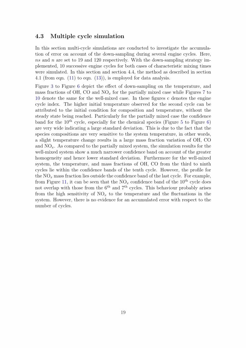
4.3 Multiple cycle simulation

In this section multi-cycle simulations are conducted to investigate the accumula-tion of error on account of the down-sampling during several engine cycles. Here,ns and n are set to 19 and 120 respectively. With the down-sampling strategy im-plemented, 10 successive engine cycles for both cases of characteristic mixing timeswere simulated. In this section and section 4.4, the method as described in section4.1 (from eqn. (11) to eqn. (13)), is employed for data analysis.

Figure 3 to Figure 6 depict the effect of down-sampling on the temperature, andmass fractions of OH, CO and NOx for the partially mixed case while Figures 7 to10 denote the same for the well-mixed case. In these figures c denotes the enginecycle index. The higher initial temperature observed for the second cycle can beattributed to the initial condition for composition and temperature, without thesteady state being reached. Particularly for the partially mixed case the confidenceband for the 10th cycle, especially for the chemical species (Figure 5 to Figure 6)are very wide indicating a large standard deviation. This is due to the fact that thespecies compositions are very sensitive to the system temperature, in other words,a slight temperature change results in a large mass fraction variation of OH, COand NOx. As compared to the partially mixed system, the simulation results for thewell-mixed system show a much narrower confidence band on account of the greaterhomogeneity and hence lower standard deviation. Furthermore for the well-mixedsystem, the temperature, and mass fractions of OH, CO from the third to ninthcycles lie within the confidence bands of the tenth cycle. However, the profile forthe NOx mass fraction lies outside the confidence band of the last cycle. For example,from Figure 11, it can be seen that the NOx confidence band of the 10th cycle doesnot overlap with those from the 6th and 7th cycles. This behaviour probably arisesfrom the high sensitivity of NOx to the temperature and the fluctuations in thesystem. However, there is no evidence for an accumulated error with respect to thenumber of cycles.

19

0

5

10

15

-150 -100 -50 0 50 100 150

LB - c10UB - c10c3c5c8c9

CO

Mas

s F

ract

ion

x 1

03

CAD

Figure 4: Mean CO mass fraction for several engine cycles (Confidence bands plot-ted for the 10th cycle) in the partially mixed case.

1100

1200

1300

1400

1500

1600

-10 0 10 20 30 40

LB - c10UB - c10c2c3c5c8c9

Tem

pera

ture

[K]

CAD

Figure 3: Mean in-cylinder temperature for several engine cycles (Confidence bandsplotted for the 10th cycle) in the partially mixed case. c denotes theengine cycle index.

In conclusion, for both the well-mixed and partially-mixed case, the down-samplingdid not accumulate noticeable errors for the multi-cycle simulations.

20

0

1

2

3

-150 -100 -50 0 50 100 150

LB - c10UB - c10c3c5c8c9

OH

Mas

s F

ract

ion

x 1

05

CAD

Figure 5: Mean OH mass fraction for several engine cycles (Confidence bands plot-ted for the 10th cycle) in the partially mixed case.

0

2

4

6

8

-150 -100 -50 0 50 100 150

LB - c10UB - c10c3c5c8c9

NO

x M

ass

Fra

ctio

n x

105

CAD

Figure 6: Mean NOx mass fraction for several engine cycles (Confidence bandsplotted for the 10th cycle) in the partially mixed case.

21

1500

1550

1600

1650

1700

-10 -5 0 5 10 15

LB - c10UB - c10c2c3c5c8c9

Tem

pera

ture

[K]

CAD

Figure 7: Mean in-cylinder temperature for several engine cycles (Confidence bandsplotted for the 10th cycle) in the well-mixed case.

6

8

10

12

-12 -11 -10 -9 -8 -7 -6 -5

LB - c10UB - c10c3c5c8c9

CO

Mas

s F

ract

ion

x 1

03

CAD

Figure 8: Mean CO mass fraction for several engine cycles (Confidence bands plot-ted for the 10th cycle) in the well-mixed case.

22

2

2.5

3

3.5

-5 0 5 10

LB - c10UB - c10c3c5c8c9

OH

Mas

s F

ract

ion

x 1

05

CAD

Figure 9: Mean OH mass fraction for several engine cycles (Confidence bands plot-ted for the 10th cycle) in the well-mixed case.

0

0.5

1

1.5

-50 0 50 100 150

LB - c10UB - c10c3c5c8c9

NO

x M

ass

Fra

ctio

n x

107

CAD

Figure 10: Mean NOx mass fraction for several engine cycles (Confidence bandsplotted for the 10th cycle) in the well-mixed case.

23

0

0.5

1

1.5

-100 -50 0 50 100 150

LB - c6UB - c6LB - c7UB - c7LB - c10UB - c10

NO

x M

ass

Fra

ctio

n x

107

CAD

Figure 11: The confidence band of the tenth-cycle NOx mass fraction versus the6th and 7th cycles in the well-mixed case.

4.4 Down-sampling: efficiency gains

In order to evaluate the effect of the introduction of the down-sampling algorithminto the SRM-DI model the simulation results obtained with and without the down-sampling algorithm implemented were compared. Influence on the computationalexpense and the error caused by down-sampling for the partially mixed and well-mixed systems were also studied. We define the down-sampling factor M as theparticle reduction ratio, i.e. M := N/n, where N and n are the number of particlesbefore and after down-sampling respectively.

Figure 12 and Figure 13 summarize the simulated results for the partially mixed andwell-mixed systems respectively. The results in both figures demonstrate that intro-ducing the down-sampling strategy into the SRM-DI did not constitute a significantcompromise of the accuracy of the simulation. The simulated results obtained withthe down-sampling factor, 3 and 5 were nearly within the confidence band deter-mined with M = 1 ( i.e. base case). However, when M was increased, e.g. 9.3,the profiles of scalar variables overlapped with the confidence bands of the corre-sponding variables for the base case. Therefore, overall it can be concluded that thedown-sampling procedure is acceptable in the simulation of a HCCI engine undergiven conditions, although larger down-sampling factors led to higher error.

Furthermore, the computational costs with and without down-sampling are com-pared and the results are listed in Table 4. It can be seen from Table 4 that withinan acceptable error, the introduction of the down-sampling strategy can speed up thesimulation approximately 8 times for both partially mixed and well-mixed systems.

24

1500

1600

1700

-10 -5 0 5 10 15 20

LB - Base caseUB - Base caseM=3M=5M=9.3

Tem

pera

ture

[K]

CAD

(a)

2

3

4

-10 -5 0 5 10 15

LB - Base caseUB - Base caseM=3M=5M=9.3

OH

Mas

s F

ract

ion

x 10

5

CAD

(b)

0

4

8

12

-50 0 50 100 150

LB - Base caseUB - Base caseM=3M=5M=9.3

CO

Mas

s F

ract

ion

x 1

03

CAD

(c)

0

0.5

1

1.5

2

-50 0 50 100 150

LB - Base caseUB - Base caseM=3M=5M=9.3

NO

x M

ass

Fra

ctio

n x

107

CAD

(d)

Figure 12: Effect of the down-sampling on the simulated properties of the gas mix-ture in the well-mixed case (τm = 2.0 × 10−4s) : (a) temperature, (b)OH mass fraction, (c) CO mass fraction, (d) NOx mass fraction.

25

1300

1400

1500

1600

-10 -5 0 5 10 15 20

LB - Base caseUB - Base caseM=3M=5M=9.3

Tem

pera

ture

[K]

CAD

(a)

1

2

3

4

5

-10 -5 0 5 10

LB - Base caseUB - Base caseM=3M=5M=9.3

OH

Mas

s F

ract

ion

x 1

06

CAD

(b)

0

4

8

12

-50 0 50 100 150

LB - Base caseUB - Base caseM=3M=5M=9.3

CO

Mas

s F

ract

ion

x 1

03

CAD

(c)

0

4

8

12

-150 -100 -50 0 50 100 150

LB - Base caseUB - Base caseM=3M=5M=9.3

NO

x M

ass

Fra

ctio

n x

108

CAD

(d)

Figure 13: Effect of the down-sampling on the simulated properties of the gas mix-ture in the partially mixed case ( τm = 2.0× 10−2s) : (a) temperature,(b) OH mass fraction, (c) CO mass fraction, (d) NOx mass fraction.

26

Table 4: The comparison of computational time for well-mixed and partially mixedsystems

CPU Time (mins)Simulation Case Factor M τm = 2× 10−2s τm = 2× 10−4s

Base Case(N = n = 334) 1 705 252Down-sampling(n = 111) 3 237 86Down-sampling(n = 66) 5 138 47Down-sampling(n = 36) 9.3 83 30

In the next section, the model is used to predict the effect of engine parameters onHCCI combustion and emissions.

5 Effects of Relative Air-fuel Ratio and Injection

Timing on Combustion

In order to control HCCI engine operation, several approaches have been investi-gated, for example, changing relative air-fuel ratio, injection timing, IVO timing,EVC timing, engine speed, boost pressure, intake gas temperature etc. as well ashybrid methods involving the integration of these strategies. With the current de-velopment of the SRM-DI model, not all mentioned strategies can be investigated inthis work. We focus on evaluating the effect of two specific engine strategies, namely,varying relative air-fuel ratio and direct injection timing. For studying these twoparameters, the model predictions will be compared with the experiment data qual-itatively. As compared to the partially mixed case, the well-mixed case providesa better representation of the volume averaged mixing time (obtained from CFDcalculations) for the two-stroke engine operation considered here. Hence, the wellmixed case is chosen for the engine parametric studies in the next section.

5.1 Relative air-fuel ratio

HCCI combustion ignition is influenced by the temperature, the pressure and thespecies mass fractions of the mixture in the cylinder. The strategies of varyingrelative air-fuel ratio (λ) influence the fuel concentration directly. Generally, thistechnique is integrated with injection timing, injection method, EGR valve timing,engine speed etc. to operate the HCCI engine.

In this section, HCCI combustion with early single-stage injection was investigatedwhile relative air-fuel ratio was varied from 2.3 to 5.6. The results are shown inFigure 14.

It can be observed that as λ decreases, the peak temperature, the peak pressure, themass fraction of NOx increase while CO mass fraction decreases. When λ reaches

27

1000

1200

1400

1600

1800

2000

-20 -10 0 10 20 30

λ = 5.6λ = 4.7λ = 3.5λ = 2.8λ = 2.3

T [

K]

CAD

(a)

4

5

6

7

8

9

-16 -14 -12 -10 -8 -6

λ = 5.6λ = 4.7λ = 3.5λ = 2.8λ = 2.3

p [

106 N

/m2 ]

CAD

(b)

4

5

6

7

8

9

-16 -14 -12 -10 -8 -6

λ = 5.6λ = 4.7λ = 3.5λ = 2.8λ = 2.3

p [

106 N

/m2 ]

CAD

(c)

10-12

10-11

10-10

10-9

10-8

10-7

10-6

10-5

10-4

-50 0 50 100 150

λ = 5.6λ = 4.7λ = 3.5λ = 2.8λ = 2.3

NO

x Mas

s F

ract

ion

CAD

(d)

Figure 14: Effect of the air-fuel ratio on the mixture’s properties in the well-mixedcase: (a) temperature, (b) pressure, (c) CO mass fraction, (d) NOx

mass fraction.

28

to 2.3, the maximum pressure gradient is higher than 15 bar/CAD, this could causeengine knock and high NOx emissions. On the other hand, when λ is too high, i.e.fuel is too lean, and hence, the mixture can not be burnt completely. It leads tohigh CO concentration. These trends match well with the experimental data in ref.(Urushihara et al., 2003; Wang et al., 2005).

5.2 Direct injection timing

In this section, the effect of varying SOI is studied. As the injection is well beforeTDC the mixture is almost homogeneous before the ignition is triggered.

Figure 15 shows that for the range of injection timings chosen the properties of themixture do not vary significantly. For example, for the cases with SOI 170 CADand 180 CAD, the profiles for the scalar properties overlap. This is due to greaterhomogeneity for these two cases. Later injection (SOI equals 190 CAD and 200CAD) causes relatively more inhomogeneity and results in a slightly higher peaktemperatures and NOx mass fraction. This predicted trend matches the experimen-tal observations by Sjoberg et al. (Sjoberg et al., 2002).

To study the effect of late direct injection, a more sophisticated treatment of themixing than what the IEM model provides is necessary. In particular localness of thescalars needs to be accounted for. However, the new SRM-DI model qualitativelypredicted the effects of variation in the relative air-fuel ratio and the early directinjection timing on HCCI combustion and emissions.

6 Conclusions

A novel SRM-DI model based on the probability density function (PDF) approachwas formulated to simulate a direct injection HCCI engine operation. With theincorporation of the gas exchange processes, the computational expense increasedrapidly. Hence, a conservative down-sampling procedure combined with a weighted-particle Monte Carlo method was developed to reduce the number of particles whileconserving the statistical properties of the ensemble.

A systematic numerical investigation of the model performance with respect to thevarious numerical parameters was carried out. It was observed that the algorithmwas more sensitive to the number of particles than the number of conserved chemicalspecies. Furthermore, multiple cycle simulation studies demonstrated that the errordue to down-sampling was not accumulated with respect to the number of enginecycles. Additionally, implementing the down-sampling technique in an engine cyclesimulation resulted in a speed-up by a factor of 8, without incurring significant errorin the numerical solution.

Model predictions for the effects of varying the relative air-fuel ratio and directinjection timing on HCCI combustion and emissions agreed with the qualitative

29

600

900

1200

1500

1800

-50 0 50 100

SOI - 170SOI - 180SOI - 190SOI - 200

T [

K]

CAD

(a)

7.5

8.0

8.5

-10 -8 -6 -4 -2 0 2

SOI - 170SOI - 180SOI - 190SOI - 200

p [

106 N

/m2 ]

CAD

(b)

5

10

15

-14 -13 -12 -11 -10 -9 -8

SOI - 170SOI - 180SOI - 190SOI - 200

CO

Mas

s F

ract

ion

x 1

03

CAD

(c)

0

2

4

6

8

10

12

0 50 100 150 200 250

SOI - 170SOI - 180SOI - 190SOI - 200

NO

x mas

s fr

acti

on

x 1

07

CAD

(d)

Figure 15: Effect of the early direct injection timing on the mixture’s propertiesin the well-mixed case: (a) temperature, (b) pressure, (c) CO massfraction, (d) NOx mass fraction.

30

trends observed in measurements elsewhere.

The framework built here can now be used to formulate an advanced model for simu-lating multiple and late direct injection HCCI combustion. Currently the efforts arebeing focussed at developing detailed sub-models for spray injection and turbulentmixing to improve the predictive power of the model.

A Appendix

Consider an ensemble of particles which are characterized by the s+1−dimensionalvector of internal parameters ψ = (ψ(1), ψ(2), ..., ψ(s+1)), where ψ(i) can be mass,momentum or energy of the particle or mass of a chemical component which theparticle contains. The ensemble is described by the mass density function F(ψ) =ρ(ψ)f(ψ). Throughout this section, we drop the time dependencies from all thenotations.

The main idea of the Monte Carlo method is the representation of the ensemble ofa large number of the physical particles by an ensemble of relatively small numberN of the computational particles such that a group of W identical molecules orparticles in the physical system is substituted by one computational particle. Theparameter W (i) is the statistical weight of the ith computational particle. In otherwords the function F(ψ) is replaced by a weighted sum of delta function as givenin eqn. (7)

Usually, the Monte Carlo method is used for estimation of the following linear func-tionals

Z(F(ψ)) =

∫F(ψ)z(ψ)dψ ≈

N∑i=1

W (i)z(ψ(i)), (14)

where z(ψ) is an integrable function. Generally speaking, the estimation (14) is arandom variable and varies from one run of the Monte Carlo algorithm to other,but some of them such as mass, momentum and energy are conserved variables andremain constant. If a Monte Carlo algorithm does not conserve these values it suf-fers from large unphysical oscillations. The proposed algorithm aims to avoid thissituation.As the number of particles in the system becomes too large, some of them have tobe removed and their statistical weights to be redistributed over the remaining par-ticles. Our purpose is to construct an algorithm that keeps the distribution function(eqn. (7)) statistically intact and also conserves physically important statisticalmoments. Below we describe the restrictions which have to be imposed on suchtransformations.First of all, the statistical weights are always non-negative:

W (i) > 0. (15)

In order to formulate the second condition define ns statistically important func-tionals Zj(F(ψ)) =

∫ F(ψ)zj(ψ)dψ, where j = 1, . . . , ns. Any redistribution of the

31

W1

W2

W3

O

A

B

β

α

C D

E

Figure 16: Schematic view of the down-sampling algorithm, the dimension of thespace N = 3 and the number of the constraints (16) is ns = 1.

statistical weights cannot affect the estimation (14). Thus W (i) satisfy the systemof linear equalities:

N∑i=1

zj(ψ(i))W (i) =

N∑i=1

ΠjiW(i) = Zj (16)

We also require that the statistical weights are bounded from above:

W (i) 6 Wmax. (17)

This condition is not necessary for the method described below, but the presence offew particles with large statistical weights means that the estimation (14) is based onthese particles mainly, while the contribution of the rest of the particles is negligible.In this case the Monte Carlo method suffers from large statistical error.Eqs. (15)-(17) imply that the vector W of the statistical weights belongs to a(N − ns)-dimensional convex polygon as it schematically shown on Fig. 16. If0 < W (i) < Wmax then W belongs to the interior of the polygon, while the edgesof the polygon correspond either to W (i) = 0 or W (i) = Wmax. An interior point ofthe convex polygon O can be represented as a linear combination of two points thatbelong to the edges:

O = pA + (1− p)B, 0 < p < 1.

Interpretation of p in the above equation as a probability yields the algorithm forthe reduction of the number of particles:

32

1. Generate a uniformly distributed unit vector g.

2. We want to replace the vector W by W = W + bg, where b is a scalar. Thus,in order to satisfy Eq. (16) the vector g has to be orthogonal to the subspaceformed by the columns of the matrix Π. Thus we recalculate g as

g := g − Π(ΠT Π)−1ΠT g.

Direct calculation shows that after this transformation ΠT g = 0.

3. Find

α = min

{ming(i)<0

{−W (i)

g(i)}, min

g(i)>0{Wmax −W (i)

g(i)}}

.

4. Find

β = min

{ming(i)>0

{W (i)

g(i)}, min

g(i)<0{W (i) −Wmax

g(i)}}

.

5. With probability β/(α + β) choose the point A, i.e., replace the vector W byW = W + αg.

6. Otherwise choose the point B: W = W − βg.

After one iteration of the above algorithm, Eq. (14) becomes:

Z1(F(ψ)) ≈N∑

i=1

(W (i) + αg(i))z(ψ(i)),

with probability β/(α + β), or

Z2(F(ψ)) ≈N∑

i=1

(Wi − βgi)z(ψ(i))

with probability α/(α + β). Direct calculation shows that

〈Z(F(ψ))〉 =β

α + βZ1(F(ψ)) +

α

α + βZ2(F(ψ)) = Z(F(ψ))

and the estimation (14) remains statistically intact for arbitrary z(ψ), while thestatistical weights of one of the particles is either 0 or Wmax.

We repeat this procedure N − ns times until the algorithm reaches a corner pointof the polygon, i.e., if we choose the point A then at the next iteration we chooserandomly between the points C and E, while if we choose the point B then wehave to choose between the points C and D. The performance of the proposedalgorithm is illustrated on Fig. 17. We randomly generated an ensemble of N = 100particles which consist of 6 components, the masses of the components in a particleare uniformly distributed from 0 to 1. As one can see, only 6 particles have weightsbetween 0 and 5 that corresponds to the number of the conserved scalars. Creationof a particle with weight Wmax has to be balanced by removal of Wmax − 1 otherparticles, since in the present case Wmax = 5, the number of the particles with weightWmax is to the number of the particles with weight 0 as 17/77 ≈ 1/5.

33

0 20 40 60 80 1000

1

2

3

4

5

i

Wi

Figure 17: Statistical weights of an ensemble of N = 100 particles after the down-

sampling. Initial statistical weights are W (i) = 1, i = 1, . . . , N , Wmax =5 and the number of the constraints (16) is ns = 6.

References

A. Bhave, M. Balthasar, M. Kraft, and F. Mauss. Analysis of a natural gas fuelledhomogeneous charge compression ignition engine with exhaust gas recirculationusing a stochastic reactor model. Int. J. Engine Res., 5(1):93–103, 2004a.

A. Bhave and M. Kraft. Partially stirred reactor model: Analytical solutions andnumerical convergence study of a PDF/Monte Carlo method. SIAM J. Sci. Com-put., 25(5):1798–1823, 2004.

A. Bhave, M. Kraft, F. Mauss, A. Oakley, and H. Zhao. Evaluating the EGR-AFRoperating range of a HCCI engine. SAE paper, No. 2005-01-0161, 2005.

A. Bhave, M. Kraft, L. Montorsi, and F. Mauss. Modelling a dual-fuelled multi-cylinder HCCI engine using a PDF-based engine cycle simulator. SAE paper, No.2004-01-0561, 2004b.

J. Y. Chen. Stochastic modeling of partially stirred reactors. Combust. Sci. andTech., 122:63–94, 1997.

S. M. Correa and M. E. Braaten. Parallel simulations of partially stirred methanecombustion. Combust. Flame, 94:469–486, 1993.

34

M. Guenthner, W. Sauter, F. Schwarz, A. Velji, and U. Spicher. A study of theignition and combustion process in a gasoline HCCI engine using port and directfuel injection. 6th International Symposium on Diagnostics and Modeling of Com-bustion in Internal Combustion Engines (COMODIA) 2004, Yokohama, Japan,2004.

R. Hasegawa and H. Yanagihara. Development of ignition control in HCCI DI dieselengine. SAE paper, No. 2003-01-0745, 2003.

R. Jhavar and J. Christopher. Effects of mixing on early injection diesel combustion.SAE paper, No. 2003-01-0154, 2005.

M. Kraft, P. Maigaard, F. Mauss, M. Christensen, and B. Johansson. Invesiti-gation of comubstion emissions in a homogeneous charge compression injectionengine: Measurements and a new computational model. Proc. Combust. Inst., 28:11951201, 2000.

B. Leach, H. Zhao, Y. Li, and T. Ma. Control of CAI combustion through injectiontiming in a GDI engine with an air-assisted injector. SAE paper, No. 2005-01-0134, 2005.

G. Lechner, T. Jacobs, C. Chryssakis, D. Assanis, and R. Siewert. Evaluation of anarrow spray cone angle, advanced injection timing strategy to achieve partiallypremixed compression ignition combustion in a diesel engine. SAE paper, No.2005-01-0167, 2005.

P. Maigaard, F. Mauss, and M. Kraft. Homogeneous charge compression ignitionengine: A simulation study on the effects of inhomogeneities. J. Eng. Gas TurbinesPower, 125:466–471, 2003.

K. Narayanaswamy, R.P Hessel, and C. J. Rutland. A new approach to modelDI-diesel HCCI combustion for use in cycle simulation studies. SAE paper, No.2005-01-3743, 2005.

K. Narayanaswamy and C. J. Rutland. Cycle simulation diesel HCCI modellingstudies and control. SAE paper, No. 2004-01-2997, 2004.

Y. Nishijima, Y. Asaumi, and Y. Aoyagi. Impingement spray system with directwater injection for premixed lean diesel combustion control. SAE paper, No.2002-01-0109, 2002.

S. B. Pope. PDF methods for turbulent reactive flows. Prog. Energy Combust. Sci.,11:119–192, 1985.

Y. Ra and R. D. Reitz. The use of variable geometry sprays with low pressureinjection for optimization of diesel HCCI engine combustion. SAE paper, No.2005-01-0148, 2005.

35

M. Sjoberg, L. Edling, T. Eliassen, L. Magnusson, and H. Angstrom. GDI HCCI:Effects of injection timing and air swirl on fuel stratification, combustion andemissions formation. SAE paper, No. 2002-01-0106, 2002.

R. Standing, N. Kalian, T. Ma, H. Zhao, M. Wirth, and A. Schamel. Effects of in-jection timing and valve timings on CAI operation in a multi-cylinder DI gasolineengine. SAE paper, No. 2005-01-0132, 2005.

G. Strang. On the construction and comparison of difference schemes. SIAM J.Numer. Anal., 5(3):506–517, 1968.

W. Su, H. Wang, and B. Liu. Injection mode modulation for HCCI diesel combus-tion. SAE paper, No. 2005-01-0117, 2005.

F. Tao, Y. Liu, B. RempelEwert, D. Foster, R. Reitz, D. Choi, and P. Miles. Mod-eling the effects of EGR and injection pressure on soot formation in a high-speeddirect-injection (HSDI) diesel engine using a multi-step phenomenological sootmodel. SAE paper, No. 2005-01-0121, 2005.

T. Tomoda, M. Kubota, R. Shimizu, and Y. Nomura. Numerical analysis of mixtureformation of a direct injection gasoline engine. 5th International Symposium onDiagnostics and Modeling of Combustion in Internal Combustion Engines (CO-MODIA) 2001, Nagoya, Japan, 2001.

T. Urushihara, K. Hiraya, A. Kakuhou, and T. Itoh. Expansion of HCCI operatingregion by the combination of direct fuel injection, negative valve overlap andinternal fuel reformation. SAE paper, No. 2003-01-0749, 2003.

A. Vikhansky and M. Kraft. Conservative method for the reduction of the number ofparticles in the Monte Carlo simulation method for kinetic equations. J. Comput.Phys., (203):371–378, 2005.

Z. Wang, J. Wang, S. Shuai, and Q. Ma. Effects of spark ignition and stratifiedcharge on gasoline HCCI combustion with direct injection. SAE paper, No. 2005-01-0137, 2005.

B. Yang and S. B. Pope. An investigation of the accuracy of manifold methods andsplitting schemes in the computational implementation of combustion chemistry.Combust. Flame, 112:16–32, 1998.

F. Zhao, T. Asmus, D. Assanis, J. Dec, J. Eng, and P. Najt. Homogeneous ChargeCompression Ignition (HCCI) Engines Key Research and Development Issues.Society of Automotive Engineers,U.S., 2003. ISBN 076801123X.

36

Acknowledgement

We express our sincere thanks to Toyota Motor Co. Japan for providing the financialsupport for the research work. Authors (HS and AB) would also like to thank theCentre for Scientific Enterprise Limited (CSEL) for the fellowship-funding. Thanksare due to our colleagues at the Computational Modelling Group, University ofCambridge for their help with the manuscript.

37