calibration and data elaboration procedure for sky irradiance measurements

Calibration and data elaborationprocedure for sky irradiance measurements

Paolo Boi, Glauco Tonna, Giuseppe Dalu, Teruyuki Nakajima, Bruno Olivieri,Alberto Pompei, Monica Campanelli, and R. Rao

The problems encountered in the elaboration of measurements of direct and sky diffuse solar irradianceare the following: ~1! to carry out the calibration for the direct irradiance, which consists in determiningthe direct irradiance at the upper limit of the atmosphere; ~2! to carry out the calibration for the diffuseirradiance, which consists in determining the solid viewing angle of the sky radiometer; ~3! to determinethe input parameters, namely, ground albedo, real and imaginary parts of the aerosol refractive index,and aerosol radius range; and ~4! to determine from the optical data the columnar aerosol optical depthand volume radius distribution. With experimental data and numerical simulations a procedure isshown that enables one to carry out the two calibrations needed for the sky radiometer, to determine abest estimate of the input parameters, and, finally, to obtain the average features of the atmosphericaerosols. An interesting finding is that inversion of only data of diffuse irradiance yields the sameaccuracy of result as data of both diffuse and direct irradiance; in this case, only calibration of the solidviewing angle of the sky radiometer is needed, thus shortening the elaboration procedure. Measure-ments were carried out in the Western Mediterranean Sea ~Italy!, in Tokyo ~Japan!, and in Ushuaia~Tierra del Fuego, Argentina!; data were elaborated with a new software package, the Skyrad code, basedon an efficient radiative transfer scheme. © 1999 Optical Society of America

OCIS codes: 010.1110, 010.1290.

rTcttMasl

tt

msmna

1. Introduction

Retrieval algorithms set up to determine atmosphericaerosol characteristics from satellite data need vali-dation so they can be tested and improved; ground-based measurements of solar radiation are the mostappropriate for such a task.1

The parameters that characterize the optical prop-erties of the atmospheric aerosol ~volume radius dis-

P. Boi and A. Pompei are with the Department of Physics, Uni-versity of Cagliari, via Ospedale 72, 09124 Cagliari, Italy. G.Tonna, B. Olivieri, and M. Campanelli are with the Institute forAtmospheric Physics, Italian National Research Council, Tor Ver-gata Research Area, via Fosso del Cavaliere 100, 00133 Rome,Italy. The email address for M. Campanelli is [email protected]. G. Dalu is with the Area della Ricerca di Cagliari,Consiglio Nazionale delle Ricerche, via V. Bottego 7, 09125 Cagli-ari, Italy. T. Nakajima is with the Center for Climate SystemsResearch, University of Tokyo, 4-6-1 Komaba, Maguro-ku, Tokyo153, Japan. R. Rao is with the Anhui Institute of Optics and FineMechanics, Chinese Academy of Sciences, Hefei, Anhui 230031,China.

Received 27 October 1997; revised manuscript received 12 No-vember 1998.

0003-6935y99y060896-12$15.00y0© 1999 Optical Society of America

896 APPLIED OPTICS y Vol. 38, No. 6 y 20 February 1999

tribution, optical depth, and complex refractiveindex! can be determined from measurements of di-ect and diffuse solar irradiance from the ground.he sky radiometer used for such measurementsomprises a telescope with annexed interferential fil-ers for the selection of the operating wavelengths inhe relevant range from l 5 0.30 to l 5 1.05 mm.easurements are usually carried out in the solar

lmucantar, that is, pointing the sky along a conicalurface with the same zenith angle as the Sun andetting the azimuthal angle vary.

The optical quantities considered in our scheme arehe direct solar irradiance F and the ratio R betweenhe sky’s diffuse irradiance, E, and F. The connec-

tion between the optical measurements and the aero-sol features occurs through the radiative transferequation in a multiple-scattering scheme. A new ef-ficient software for analyzing the data, the Skyrad~sky radiation! code, was presented by Nakajima etal.2; it permits elaboration of data on both R and F

easurements ~mode INDM 5 0, where INDMtands for index M! as well as of data on R measure-ents only ~mode INDM 5 2!. Input parameterseeded before the inversion begins are the minimumnd maximum radii of the aerosol, rm and rM, respec-

tively; the complex refractive index of the aerosol, m

b

K

Ssvmafw

wemat

uPkwafaa0

r

5 m 2 ik; and the spectral ground albedo, A. Twocalibration parameters for F and R have to be deter-mined when the mode INDM 5 0 is used; only cali-ration for R is needed with mode INDM 5 2.The Skyrad code was used in previous research.aufman et al.3 carried out measurements in several

geographical regions with a sky radiometer operatingat eight spectral bands for direct irradiance measure-ments ~from 0.44 to 1.03 mm! and at three spectralbands ~0.44, 0.62, and 0.87 mm! for sky irradiancemeasurements in the almucantar. R data for scat-tering angles in the range 2° # Q # 40° were used toretrieve ~INDM 5 2! the aerosol volume radius dis-tribution in the radius interval 0.06 , r , 10 mm;bimodal and trimodal spectra were found. The aero-sol optical depth tA was determined both from only Fdata by use of a normal Langley plot and from only Rdata. In the elaboration of data, characteristic val-ues were assumed for the m, k, and A input param-eters; fixed values were taken for rm and rM. Dalu etal.4 carried out measurements in Sardinia, Italy,within the wavelength range from 0.369 to 1.048 mm.Optical R data were elaborated with mode INDM 5 2in the 3° # Q # 35° interval. The aerosol volumespectra obtained indicated a trimodal distribution,with mode radii located at ;0.15, ;0.5, and ;2 mm;the diurnal behavior of tA was also determined. Forrm and rM the fixed values 0.01 and 10 mm were used.

everal values for input parameters m, k, and A wereelected for the computations, and an optimal set ofalues was determined at each hour from the mini-um shown by e#~R!, a residual of the retrieved R data

veraged over wavelength. The parameter e#~R! wasound to depend rather strongly on m and onlyeakly on k and A. Tonna et al.5 demonstrated,

with numerical simulations for mode INDM 5 2, thatinaccurate values of the input parameters can causelarge errors in the results, whereas at the same timethe parameter e#~R! changes only slightly. Nakajimaet al.2 anticipated a possible procedure for determin-ing the calibration constants and the input parame-ters from the optical data rather than from additionalmeasurements.

In this paper we use measurements, as well asnumerical simulations, to present the elaborationprocedure that was set up during the past four yearsand used by our research group for elaborating opti-cal data taken in Italy, Japan, and Argentina.

2. Measured Quantities and Data Inversion

The quantities measured in a cloudless sky, with so-lar radiation as the source, are direct and sky diffuseirradiances. The direct solar spectral irradiance F~W m22 mm21! is given by6

F 5 F0 exp~2m0t!, (1)

where F0 is the irradiance at the upper limit of theatmosphere, t is the total optical depth; u0 is the Sun’szenith angle; and m0 is the relative optical air mass,which is expressed approximately as m0 5 1ycos u0for u0 , 60° ~more-accurate values are given in Ref. 7

for any u0 value!. The total optical depth t is thesum of the optical depths for aerosol ~tA! and mole-cules ~tm!. The sky’s diffuse irradiance E ~W m22

mm21! is assumed here as normalized by direct irra-diance; this ratio, for a one-layer plane-parallel at-mosphere in the almucantar, is given by6

R~Q! ;E~Q!

Fm0DV5 vtP~Q! 1 r~Q! ; b~Q! 1 r~Q!, (2)

here DV is the solid view angle of the sky radiom-ter, v is the single-scattering albedo of the whole airass, P~Q! is the total phase function at scattering

ngle Q, b~Q! [ vtP~Q! is the total differential scat-ering coefficient, and r~Q! is the total multiple-

scattering contribution. Scattering coefficient b isthe sum of the scattering coefficients for aerosol ~bA 5vAtAPA! and for molecules ~bm 5 vmtmPm!, wherevA, PA and vm, Pm are the single-scattering albedoand phase function for aerosol and molecules, respec-tively. The connection between Q and the zenithand azimuth angles of observation u0 and f is ex-pressed as cos Q 5 cos2 u0 1 sin2 u0 cos f in thealmucantar; the limit for Q is 0° # Q # 2u0.

The two types of sky radiometer ~aureolemeter!sed in our research program, models Pom-01 andom-01L manufactured by the Prede Company, To-yo, measure the F and E irradiances at six and fouravelengths, respectively, selected within the maintmospheric windows in the visible and the near in-rared. The wavelengths for the Pom-01 radiometerre 0.369, 0.500, 0.675, 0.776, 0.862 and 1.048 mm,nd those for the Pom-01L instrument are l 5 0.400,.500, 0.870, 1.040 mm, hereafter denoted l1, l2, . . . .

Actually, the 0.500- and 0.675-mm wavelengths haveozone extinction components and the 1.040- and1.048-mm wavelengths are contaminated by thewater-vapor absorption continuum. On the otherhand, as the aerosol extinction dominates in our mea-surements and our analysis is based mainly on nor-malized radiance R, which numerical simulationshave shown is insensitive to small gaseous absorp-tion, we have deemed it reasonable at present to treatthe radiative transfer problem as a pure scatteringproblem ~see Section 5 below!. The field of view ofthe radiometers is ;1°; the minimum angle for scat-tering measurements is assumed to be 3°, because forQ $ 3° the contamination by stray light is not signif-icant for our application.

If the voltage outputs for F, F0, and E are given byV, V0, and VE, respectively, Eqs. ~1! and ~2! can beewritten as

V 5 V0 exp~2m0t!, (3)

R~Q! ;VE

Vm0DV5 b~Q! 1 r~Q!. (4)

Equations ~1!–~4! are strictly monochromatic andhave to be used for small bandpass. HereafterR~l1!, R~l2!, . . . will be denoted as R1, R2, . . . , re-spectively.

20 February 1999 y Vol. 38, No. 6 y APPLIED OPTICS 897

i

ddt~

o

ss0iI3f

s3r

ampt

8

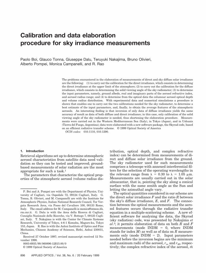
The inversion of the measured optical data is car-ried out with the REDML ~reduced multiple scatter-ng! program ~Fig. 1!, included in the Skyrad code,

whose main subroutine is RTRN1 ~radiative transfercode!, based on the improved multiple–single scatter-ing method2 for handling the radiative transfer equa-tion in a plane-parallel atmosphere. From R~Q!data the multiple-scattering component is removedby an iterative regression and the scattering coeffi-cient b~Q! is obtained. From b~Q! and possibly fromt data, the aerosol volume radius distribution v~r! isrecovered by the AEINV ~aureole-extinction inver-sion code! subroutine as a histogram.

The REDML program minimizes the parametere~R!, whose final value indicates the accuracyachieved in the retrieval process, defined as the rmsrelative deviation ~in percent! between the measuredR data and those reconstructed through the retrievedvolume radius distribution, averaged over the mea-surement scattering angles. Henceforth, when it isfurther averaged over wavelength, e~R! will be de-noted e#~R!.

We note that, before t and R in Eqs. ~3! and ~4!

Fig. 1. Flow chart of the REDML program for inverting data ofdirect and diffuse solar irradiance.


become available for inversion, the two calibrationparameters V0 and DV have to be determined. In-put parameters to the REDML program are rm andrM, m, k, and A; m and k are assumed to be indepen-

ent of wavelength and are averaged over the wholeay. The ground albedo A is assumed to depend onime and wavelength, so A stands for the vector A [A1, A2, . . . !; when A1 5 A2 5 . . . we speak of a single

value of A.The REDML program ~Fig. 1! can work in either of

two modes, selected by INDM:

• INDM 5 0, where t data are available and re-liable; in this case they are used together with theR~Q! data in the retrieval of v~r!. The two calibra-tion parameters V0 and DV have to be determined.

• INDM 5 2, t data are not available; in this casethe inversion relies only on R~Q! data, which we in-vert to determine v~r! and tA. In this case the cali-bration determines only the parameter DV.

The REDML program proved5 to be able to retrievethe optical and microphysical features of the colum-nar aerosol with accuracy ~within 1% of the measuredptical quantities! and efficiency ~within 10 s on the

Sun workstation Solaris 2.6! in several different sit-uations, provided that the pertinent calibration con-stants and input parameters were given. From thebehavior with r of several kernels5 concerning tA andbA, at refractive indices typical of the atmosphericaerosol it was found that the radius interval of reli-able information content is 0.03–3 mm for extinctiondata and 0.06–10 mm for scattering data in the 3° #Q # 30° interval; when measurements of normalizedky irradiance are used together with extinction mea-urements ~INDM 5 0!, this radius interval is.03–10 mm. It is seen that the information contents almost the same for the two modes, INDM 5 0 andNDM 5 2, because the kernel for scattering at Q 50° has almost the same behavior with r as the kernelor extinction.

As to the input parameters, both experimental andimulated5 data demonstrated ~INDM 5 2, 3° # Q #0°! that inaccurate values cause large errors in theesults of the inversion ~v and tA!, whereas, at the

same time, e~R! does not change; only for incorrectvalues of m does e~R! rise rapidly.

The procedure described here ~Section 3! and dem-onstrated ~Section 4! with experimental and simu-lated data allows us to determine DV, V0, m, k and A,v, and tA, mainly on the basis of mode INDM 5 2 andof only optical data, without the need for additionalmeasurements. For rm and rM we simply assumethe fixed values rm 5 0.01 mm and rM 5 10 mm.

3. Data-Elaboration Procedure

The combination of measurements of direct and dif-fuse irradiance ~INDM 5 0! is in principle the bestrrangement with respect to the number of measure-ents made and the kind of information on aerosol

articles that can be obtained. On the other hand,he determination of t from measurements of V ~t [

2 iepdo

r

tdir! according to Eq. ~3! requires determining thespectral behavior of V0, which is usually done withthe Langley plot method,8 which for each wavelengthlocates V0 on a V–m0 graph for m0 3 0 under thehypothesis that t is a constant during the calibration.This procedure omits from Eq. ~3! the dependence ofV on optical variable t and retains the dependence ongeometrical variable m0; during the measurementsthe above hypothesis cannot be fulfilled, so particularcare must be taken in implementing the Langley plot.Alternatively, one can use only R data ~INDM 5 2!and find tA accordingly ~tA [ tA

diff!.Let us suppose that we have carried out measure-

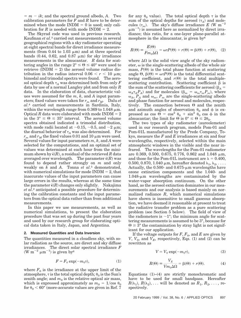
ments of both direct and diffuse irradiance for a dayat a 15-min intervals so we have approximately 30complete sets of data. The proposed procedure ~Fig.! consists of the following steps:

A. Determination of the Solid Viewing Angle

One can assume that the value of solid viewing angleDV ~Fig. 2, step 1! comes from the geometry of the

Fig. 2. Block diagram showing the procedure for data elaboration.In step 1 DV is a function of wavelength; in step 2 the R~li, Qj! dataepresent all the available sets of data; ind., indicative value of.

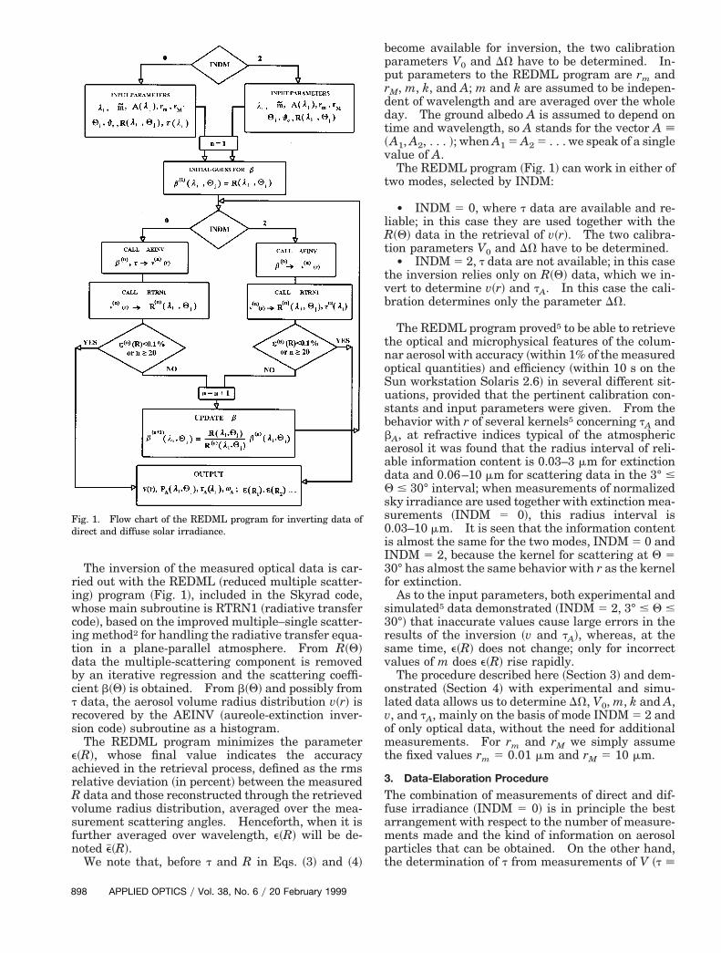
telescope. Several factors contribute to this value:color aberration of the lens, diffraction at the edges,misalignment of the optical axis, and surface nonuni-formity of filters and sensor. As a consequence, weset up a method to determine DV directly from opticaldata on the scanning of the irradiance field about theSun centered at the origin of a local system of rect-angular coordinates; the solid viewing angle is givenby

DV 5 **DA

E~x, y!

E~0, 0!dxdy, (5)

where x and y ~in radians! are polar coordinates thatdetermine the position of the optical axis with respectto the position of the Sun. Figure 3 shows the ge-ometry of the disk-scanning method. We estimatethe solid viewing angle by measuring the irradianceat 21 3 21 gridded points in zenithal and azimuthalplanes about the solar disk, with an angular resolu-tion of 0.1° and a scanning domain DA of 2° by 2°;measurements are made for all the channels of theradiometer. After correction for the movement ofthe solar disk during the scanning procedure, thesignals are registered as a function of the ~x, y! coor-dinates. Finally, to obtain the integral in Eq. ~5!, weintroduce an elliptical system of coordinates centeredat ~0, 0! and find the needed parameters by fitting themeasurements; the response function f ~x, y! 5 E~x,y!yE~0, 0! is ultimately expressed as a function of theellipse’s major semiaxis s as f ~x, y! [ f ~s!, and Eq. ~5!becomes

DV 5 2pb * f ~s!sds, (6)

where b is the ellipticity.

B. Determination of m*

An optimal value m* for m can be determined ~Fig. 2,step 2! from the minimum exhibited by e#~R! versus mn the 3° # Q # 30° interval, where the dependence of

#~R! on m is strong because of the variation of aerosolhase function PA, and hence of bA, with m, while theependence on k and A is weak. To this end each setf data is elaborated with INDM 5 2 for several val-

Fig. 3. Geometry of the solar disk scanning method.


Ao

amp

4e

i

aw

t

w

c

n

wal

At

ldam

spgtomw

mJ~n

~6

9

ues of m and for indicative values of k and A. Forconsistency with a value of k to be determined later,e#~R! versus m is further averaged, ^e#~R!&, over all thesets of data to yield one m* value for the entire day.

The real part of m is assumed to be independent ofl because e~Ri! versus the corresponding mi does notshow a clear minimum that is suitable for locating anoptimal mi* value, whereas e#~R! as a function of mdoes. Also, e~R1!, e~R2!, . . . depend simultaneouslyon m1, m2, . . . through the retrieved values of v andtA

diff and are used for reconstructing R1, R2, . . . .

C. Determination of k*

An optimal value k* for k is determined ~Fig. 2, step3! by means of a modified version9 of the Langley plot~called the direct-diffuse Langley plot!, which in Eq.~3! uses tdiff instead of the unknown tdir. To this endeach set of data is elaborated with INDM 5 2 in theinterval 3° # Q # 30° with m*, an indicative value for

, and several values of k. With the tdiff values sobtained the scatter diagram of the ~ln V, m0tdiff!

points is set up, and slope c of the straight line

ln V 5 ln V0 2 cm0tdiff (7)

is determined for each couple ~k, A!. The coefficientc depends strongly on k and only weakly on A.When the value of k is correct, coefficient c is close tounity, so an optimal value k* can be determined fromthe minimum exhibited by e#c, a rms of ~c 2 1!, aver-ged over wavelength, versus k; k* so obtained is aean of wavelength and of the entire day. By com-

aring Eqs. ~7! and ~3! we get c [ tdirytdiff, so thismethod of determining k ultimately amounts to tun-ing between measurements of direct and diffuse ir-radiance and recalls the previous method of King andHerman.10 Also, it exploits the information contentof the direct irradiance.

D. Determination of A*

An optimal value A* for A is determined ~Fig. 2, step! for each set of data from the behavior of each e~R1!,~R2!, . . . versus A in the interval 60° # Q # 90°,

because within this interval R has a strong depen-dence on A. To this end we start ~n 5 0! to recon-struct the ratios R1, R2, . . . with the results obtainedin steps 2 and 3 ~v0, tA

0 ! and several single values of A.From the minimum exhibited by each e~R1!, e~R2!, . . .versus A we find A0, the optimal value of A at the firstteration. With m*, k*, and A0 we compute

~INDM 5 2, 3° # Q # 30°! updated v and t ~v1 and t1!,nd start a new cycle. The procedure is stoppedhen for each ith component of A the difference ~Ai

n

2 Ain21! at the nth and ~n 2 1!st iterations is less

han or equal to 3%. The convergence of An towardA* usually occurs within a few cycles.

The ground albedo A was assumed to depend onavelength because only seldom does e#~R! versus A

show a behavior that is suitable for finding a uniqueA. In addition, the procedure that one uses to find A~Fig. 2, step 4! allows each e~Ri! to depend only on theorresponding mi. The determination of A* is iter-


ative in nature because, for each A , the values of vand tA are updated.

E. Determination of V*0Once we have determined m*, k*, and A* we assumethat v* [ vn11 and t*A [ tA

n11 are optimal estimates ofv~r! and tA

diff for each set of data ~Fig. 2, step 5!. Nowe can go directly to the end ~switch 1 off !, or set updirect-diffuse Langley plot ~switch 1 on!, which al-

ows us ~Fig. 2, step 6! to determine V*0 correctly alonga fitted line given by Eq. ~3! and finally to derive tA

dir.s a check on the quality of measurements, calibra-

ions, and inversion procedure we can compare tAdir

with tAdiff.

We can now go to the end ~switch 2 off ! or ~switch2 on! to assume that t is the same as tdir ~Fig. 2, step7! and to invert R and tdir data with mode INDM 5 0with input data m*, k*, and A*, and to obtain v**,which is possibly a better estimate of v than v*.

The last two steps ~Fig. 2, steps 6 and 7! proved notto be strictly necessary to the procedure, as they donot actually improve the results previously obtainedin step 5; this is so because we have already used theinformation content included in the data of directirradiance when we derived the direct-diffuse Lan-gley plot to find k*. As a consequence, the procedurecan be stopped after step 5 ~switch 1 off !. In thiscase the only needed calibration is to determine DV;we use the direct-diffuse Langley plot only to deter-mine k* and do not use it further to determine V*0.

This procedure was used by us with both experi-mental and simulated data, and some of the resultsare given in Section 4.

4. Results from Experimental and Simulated Data

The procedure outlined above was used by us for theelaboration of measurements carried out at two sites~Carloforte and Cagliari! in the south Sardinia ~Ita-y!, a large island in the western Mediterranean Sea,uring three summers ~1994, 1995, 1996!, as part ofEuropean project and in conjunction with measure-ents carried out in Tokyo ~Japan! and in Ushuaia

~Tierra del Fuego, Argentina!.Measurements were carried out every 15 min,

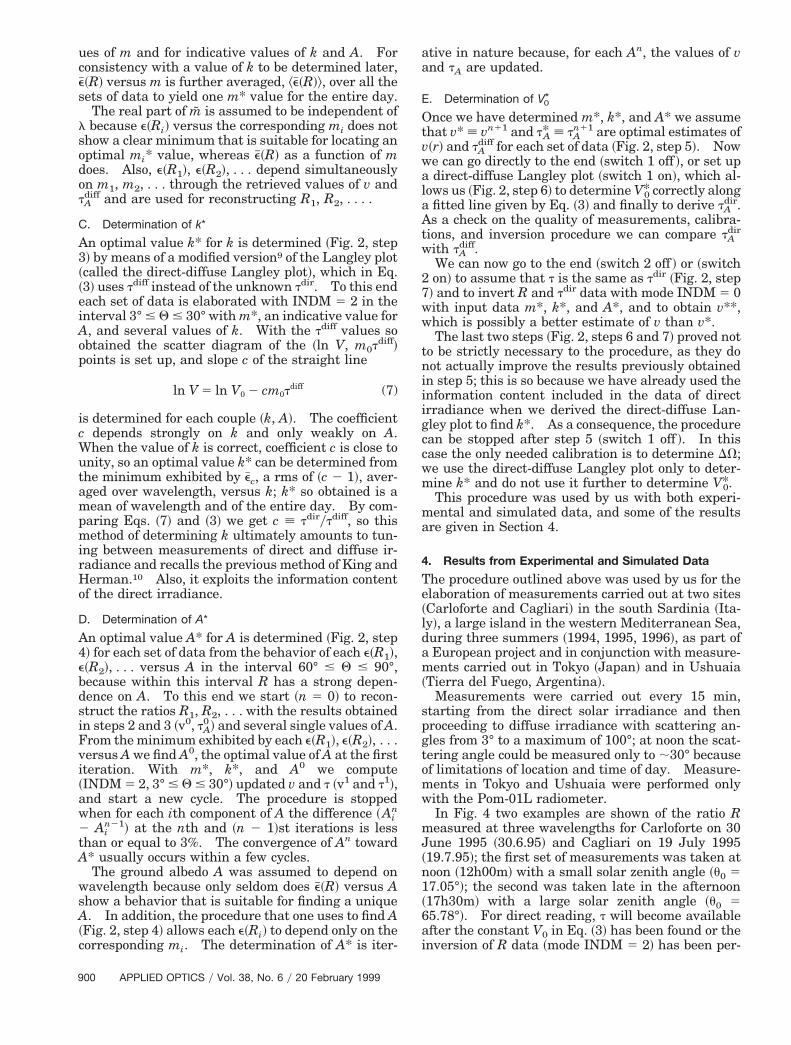
tarting from the direct solar irradiance and thenroceeding to diffuse irradiance with scattering an-les from 3° to a maximum of 100°; at noon the scat-ering angle could be measured only to ;30° becausef limitations of location and time of day. Measure-ents in Tokyo and Ushuaia were performed onlyith the Pom-01L radiometer.In Fig. 4 two examples are shown of the ratio Reasured at three wavelengths for Carloforte on 30

une 1995 ~30.6.95! and Cagliari on 19 July 199519.7.95!; the first set of measurements was taken atoon ~12h00m! with a small solar zenith angle ~u0 5

17.05°!; the second was taken late in the afternoon17h30m! with a large solar zenith angle ~u0 55.78°!. For direct reading, t will become available

after the constant V0 in Eq. ~3! has been found or theinversion of R data ~mode INDM 5 2! has been per-

riiTa

t

a35dvd5

tvs

a

c

formed; the behavior of t with wavelength will de-pend mainly on the size distribution.11

At the same time we simulated four days of mea-surements and carried out the relevant inversions.The aerosol volume radius distribution assumed forthe simulations is the sum of two log normals. Theindex of refraction was assumed as m 5 1.45 20.005i; rm and rM were taken as 0.01 and 10 mm,espectively. V and R data were simulated at timentervals of 15 min from 12h00m to 18h15m, whichmplies m0 from 1.05 to 3.5; V0 was taken as V0 [ 1.he four days were characterized as follows: firstnd fourth days, tA variable with time, A [ ~5, 5, 5, 5,

5, 5!%; second and third days, tA and A variable withime.

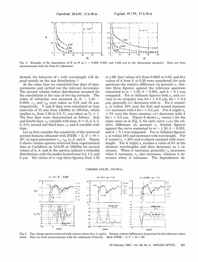
Let us first consider the sensitivity of the retrievederosol features obtained with INDM 5 2, 3° # Q #0°, to input parameters rm, rM, m, k, and A. Figureshows volume spectra retrieved from experimentalata at Carloforte on 18.6.95 at 10h00m for severalalues of m, k, and A; the spectra indicate a trimodalistribution, with the modes located near 0.2, 1.5, andmm. Six values of m ~top three figures! from 1.35

Fig. 4. Example of the dependence of R on Q at l 5 0.369,measurements with the Pom-01 radiometer.

Fig. 5. Top, volume spectra retrieved with various values of m, k, alisted. Data are from measurements with the radiometer Pom-0

o 1.60, four values of k from 0.0005 to 0.02, and fivealues of A from 0. to 0.20 were considered; for eachpectrum the relative difference ~in percent! ev ~bot-

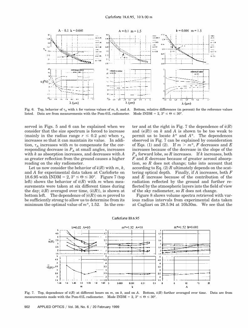
tom three figures! against the reference spectrumconnected to m 5 1.50, k 5 0.001, and A 5 0.1 wascomputed. For m ~leftmost figures! both ev and v~r!vary in an irregular way for r $ 0.2 mm; for r # 0.2mm, generally v~r! decreases with m. For k ~center!ev is within 10% near the first and second maxima;v~r! increases with k for r # 0.2 mm. For A ~right! ev# 5% near the three maxima; v~r! decreases with Afor r # 0.2 mm. Figure 6 shows tA versus l for thesame cases as in Fig. 5; for each curve tA~l! the rel-ative difference ~in percent! et ~bottom figures!gainst the curve connected to m 5 1.50, k 5 0.001,

and A 5 0.1 was computed. For m ~leftmost figures!et is within 16% and increases with wavelength. Fork ~center! et # 20% and is almost constant with wave-length. For A ~right! et reaches a value of 8% at theshortest wavelengths and then decreases as l in-reases. When m increases, generally tA increases;

when k increases, tA also increases, whereas it de-creases when A increases. The dependences ob-

, and 1.048 mm in the almucantar geometry. Data are from

. Bottom, relative differences ~in percent! for the reference valuesMode INDM 5 2, 3° # Q # 30°.

0.500

nd A1L.


r

tarflo

ia

9

served in Figs. 5 and 6 can be explained when weconsider that the size spectrum is forced to increase~mainly in the radius range r # 0.2 mm! when tAincreases so that it can maintain its value. In addi-tion, tA increases with m to compensate for the cor-esponding decrease in PA at small angles, increases

with k as absorption increases, and decreases with Aas greater reflection from the ground causes a higherreading on the sky radiometer.

Let us now consider the behavior of e#~R! with m, k,and A for experimental data taken at Carloforte on18.6.95 with INDM 5 2, 3° # Q # 30°. Figure 7 ~topleft! shows the behavior of e#~R! with m when mea-surements were taken at six different times duringthe day; e#~R! averaged over time, ê#~R!&, is shown atbottom left. The dependence of ê#~R!& on m proved tobe sufficiently strong to allow us to determine from itsminimum the optimal value of m*, 1.52. In the cen-

Fig. 6. Top, behavior of tA with l for various values of m, k, andlisted. Data are from measurements with the Pom-01L radiome

Fig. 7. Top, dependence of e#~R! at different hours on m, on k, ameasurements made with the Pom-01L radiometer. Mode INDM


ter and at the right in Fig. 7 the dependence of e#~R!and ê~R!& on k and A is shown to be too weak topermit us to locate k* and A*. The dependencesobserved in Fig. 7 can be explained by considerationof Eqs. ~1! and ~2!. If m . m*, F decreases and Eincreases because of the decrease in the slope of thePA forward lobe, so R increases. If k increases, bothF and E decrease because of greater aerosol absorp-tion, so R does not change; take into account thataccording to Eq. ~2! R ultimately depends on the scat-ering optical depth. Finally, if A increases, both Fnd E increase because of the contribution of theadiation reflected by the ground and further re-ected by the atmospheric layers into the field of viewf the sky radiometer, so R does not change.Figure 8 shows volume spectra retrieved with var-

ous radius intervals from experimental data takent Cagliari on 28.5.94 at 10h30m. We see that the

Bottom, relative differences ~in percent! for the reference valuesMode INDM 5 2, 3° # Q # 30°.

n A. Bottom, e#~R! further averaged over time. Data are from, 3° # Q # 30°.

A.ter.

nd o5 2

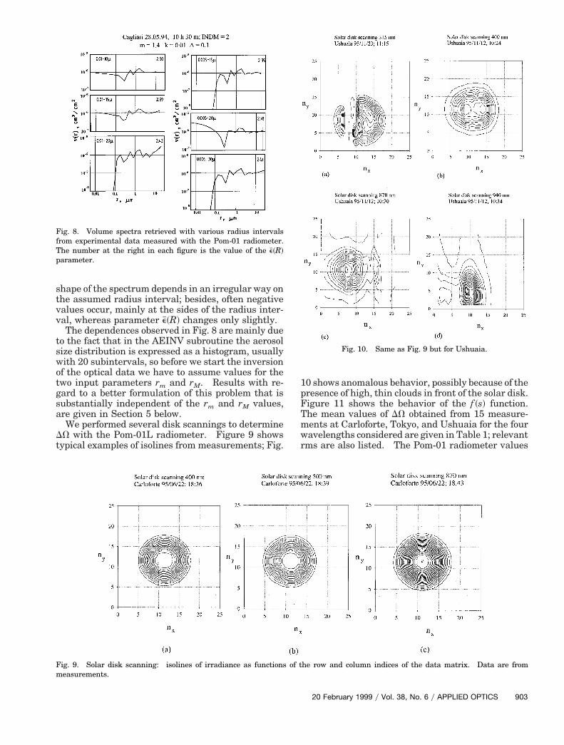
shape of the spectrum depends in an irregular way onthe assumed radius interval; besides, often negativevalues occur, mainly at the sides of the radius inter-val, whereas parameter e#~R! changes only slightly.

The dependences observed in Fig. 8 are mainly dueto the fact that in the AEINV subroutine the aerosolsize distribution is expressed as a histogram, usuallywith 20 subintervals, so before we start the inversionof the optical data we have to assume values for thetwo input parameters rm and rM. Results with re-gard to a better formulation of this problem that issubstantially independent of the rm and rM values,are given in Section 5 below.

We performed several disk scannings to determineDV with the Pom-01L radiometer. Figure 9 showstypical examples of isolines from measurements; Fig.

Fig. 8. Volume spectra retrieved with various radius intervalsfrom experimental data measured with the Pom-01 radiometer.The number at the right in each figure is the value of the e#~R!parameter.

Fig. 9. Solar disk scanning: isolines of irradiance as functionsmeasurements.

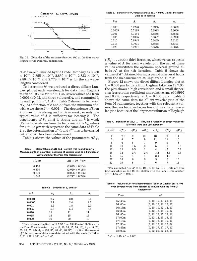
10 shows anomalous behavior, possibly because of thepresence of high, thin clouds in front of the solar disk.Figure 11 shows the behavior of the f ~s! function.The mean values of DV obtained from 15 measure-ments at Carloforte, Tokyo, and Ushuaia for the fourwavelengths considered are given in Table 1; relevantrms are also listed. The Pom-01 radiometer values

he row and column indices of the data matrix. Data are from

Fig. 10. Same as Fig. 9 but for Ushuaia.

of t


2

~

v

tsasPul

2

Table 3. Behavior of V versus k and A at l 5 0.500 mm for the Same

9

of DV were furnished by the Prede Company as 3.2303 1024, 2.855 3 1024, 2.830 3 1024, 2.833 3 1024,.804 3 1024, and 2.778 3 1024 sr for the six wave-

lengths considered.To determine k* we produced a direct-diffuse Lan-

gley plot at each wavelength for data from Cagliaritaken on 19.7.95 for m* 5 1.45, seven values of k from0.0001 to 0.02, and three values of A, and computed e#cfor each point ~m*, k, A!. Table 2 shows the behaviorof e#c as a function of k and A; from the minimum of e#cwith k we chose k* 5 0.001. The dependence of e#c onk proves to be strong and on A is weak, so only onetypical value of A is sufficient for locating k. Thedependence of V0 on A is strong and on k is weakTable 3!, as shown from the behavior of the V0 values

for l 5 0.5 mm with respect to the same data of Table2, so the determination of V0 and tdir has to be carriedout after A* has been determined.

Table 4 shows the values of the parameters e~R1!,

Fig. 11. Behavior of the response function f ~s! at the four wave-lengths of the Pom-01L radiometer.

Table 1. Mean Values of DV and Relevant rms Found from 15Measurements of Solar Disk Scanning at Various Sites as a Function of

Wavelength for the Pom-01L Radiometer

l ~mm! DV 3 1024 ~sr!

0.400 ~2.029 6 0.134!0.500 ~2.020 6 0.168!0.870 ~2.096 6 0.135!1.040 ~2.247 6 0.225!

Table 2. Behavior of e#c with Aa

k\A A1 A2 A3

0.0001 2.7 3.0 3.40.0005 2.1 2.4 2.70.001 1.7 1.8 2.00.005 5.6 5.4 5.40.010 11 11 110.015 15 15 150.020 19 20 19

aData taken at Cagliari on 19.7.95 from 13h30m to 18h00m withthe Pom-01 radiometer. A1 5 ~0, 10, 15, 15, 15, 10!, A2 5 ~5, 20,5, 25, 25, 20!, A3 5 ~10, 35, 40, 40, 40, 35!. Optical thicknesses

tAdiff for each set of data were determined with the mode INDM 5

2, 3° # Q # 30°, m* 5 1.45.


e~R2!, . . . at the third iteration, which we use to locatea value of A for each wavelength; the set of thesevalues constitutes the optimum spectral ground al-bedo An at the nth iteration. Table 5 shows thealues of A* obtained during a period of several hours

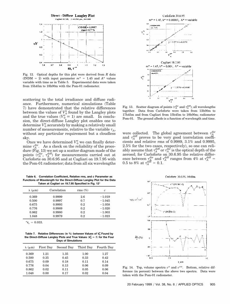
from the measurements at Cagliari on 19.7.95.Figure 12 shows the direct-diffuse Langley plot at

l 5 0.500 mm for data from Cagliari taken on 19.7.95;he plot shows a high correlation and a small disper-ion ~correlation coefficient and relative rms of 0.9997nd 0.7%, respectively, at l 5 0.500 mm!. Table 6hows the same data for all six wavelengths of theom-01 radiometer, together with the relevant c val-es; the rms becomes larger toward the shorter wave-

engths because of the larger contribution of Rayleigh

0

Data as in Table 2

k\A A1 A2 A3

0.0001 5.7226 5.6955 5.66320.0005 5.7195 5.6923 5.66060.001 5.7154 5.6885 5.65520.005 5.6995 5.6697 5.62200.010 5.6943 5.6469 5.61620.015 5.7001 5.6548 5.63030.020 5.7201 5.6545 5.6375

Table 4. Behavior of e~R1!, . . . , e~R6! as a Function of Single Values forA for the Third and Last Iterationa

A ~%! e~R1! e~R2! e~R3! e~R4! e~R5! e~R6!

0 2.6 9 10 13 13 112 4 7 9 11 11 105 6 5 7 9 9 8

10 10 1.5 3 5 6 6.812 11 0.5 2 4 5 6.815 14 2.4 2.4 3.2 4.3 7.517 15 4 4 3.4 4.5 820 18 6 6 5 6 1022 19 8 7 6 7 11

aThe estimated A is A* [ ~0, 12, 12, 15, 15, 12!. Data are fromCagliari taken at 19.7.95 at 16h30m with the Pom-01 radiometer.m* 5 1.45, k* 5 0.001.

Table 5. Values of A* for Measurements Taken at Cagliari on 19.7.95over Several Hours from 15h45m to 18h00m with the Pom-01

Radiometera

Time A*

15h45m ~0, 10, 15, 17, 20, 15!16h00m ~0, 10, 10, 12, 12, 10!16h15m ~0, 10, 10, 12, 12, 10!16h30m ~0, 12, 12, 15, 15, 12!16h45m ~0, 12, 12, 15, 15, 12!17h00m ~0, 12, 12, 15, 15, 15!17h15m ~0, 12, 12, 15, 15, 10!17h30m ~0, 12, 12, 12, 12, 5!17h45m ~0, 20, 17, 17, 17, 10!18h00m ~0, 22, 20, 22, 22, 15!

am* 5 1.45, k* 5 0.001.

7

Ct

w

t1P

scattering to the total irradiance and diffuse radi-ance. Furthermore, numerical simulations ~Table! have demonstrated that the relative differences

between the values of V*0 found by the Langley plotsand the true values ~V*0 [ 1! are small. In conclu-sion, the direct-diffuse Langley plot enables one todetermine V*0 accurately by making a relatively smallnumber of measurements, relative to the variable tA,without any particular requirement but a cloudlesssky.

Once we have determined V*0 we can finally deter-mine tA

dir. As a check on the reliability of the proce-dure ~Fig. 13! we set up a scatter diagram made of thepoints ~tA

dir, tAdiff! for measurements carried out at

arloforte on 30.6.95 and at Cagliari on 19.7.95 withhe Pom-01 radiometer; data from all six wavelengths

Fig. 12. Optical depths for this plot were derived from R data~INDM 5 2! with input parameter m* 5 1.45 and A* valuesvariable with time as in Table 5. Experimental data were takenfrom 15h45m to 18h00m with the Pom-01 radiometer.

Table 6. Correlation Coefficient, Relative rms, and c Parameter asFunctions of Wavelength for the Direct-Diffuse Langley Plot for the Data

Taken at Cagliari on 19.7.95 Specified in Fig. 12a

l ~mm! Correlation rms ~%! c

0.369 0.9999 2.6 21.0190.500 0.9997 0.7 21.0450.675 0.9993 0.2 21.0580.776 0.9989 0.2 21.0200.862 0.9980 0.2 21.0031.048 0.9979 0.2 21.023

ae#c 5 0.033.

Table 7. Relative Differences ~in %! between Values of V*0 Found bythe Direct-Diffuse Langley Plots and True Values ~V*0 [ 1! for the Four

Days of Simulations

l ~mm! First Day Second Day Third Day Fourth Day

0.369 1.21 1.35 1.00 1.270.500 0.35 0.45 0.33 0.420.675 0.09 0.18 0.11 0.140.776 0.04 0.13 0.06 0.090.862 0.02 0.11 0.05 0.061.048 0.00 0.17 0.02 0.04

ere collected. The global agreement between tAdir

and tAdiff proves to be very good ~correlation coeffi-

cients and relative rms of 0.9989, 3.1% and 0.9995,2.5% for the two cases, respectively!, so one can reli-ably assume that tA

diff or tAdir is the optical depth of the

aerosol; for Carloforte on 30.6.95 the relative differ-ence between tA

dir and tAdiff ranges from 4% at tA

diff 50.5 to 8% at tA

diff 5 0.1.

Fig. 13. Scatter diagram of points ~tAdir and tA

diff!; all wavelengthsogether. Data from Carloforte were taken from 13h00m to7h45m and from Cagliari from 15h45m to 18h00m; radiometerom-01. The ground albedo is a function of wavelength and time.

Fig. 14. Top, volume spectra v* and v**. Bottom, relative dif-ference ~in percent! between the above two spectra. Data weretaken with the Pom-01 radiometer.


iptsssdrdmdb~m

bpipmt

r

r

9

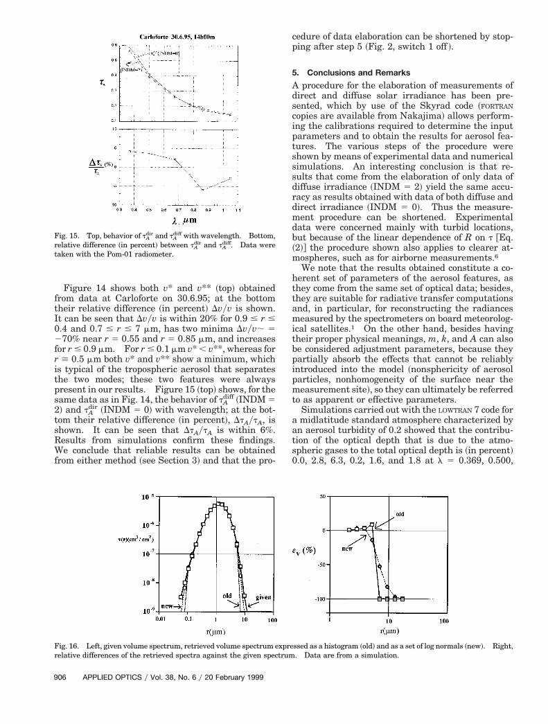
Figure 14 shows both v* and v** ~top! obtainedfrom data at Carloforte on 30.6.95; at the bottomtheir relative difference ~in percent! Dvyv is shown.It can be seen that Dvyv is within 20% for 0.9 # r #0.4 and 0.7 # r # 7 mm, has two minima Dvyv; 5270% near r 5 0.55 and r 5 0.85 mm, and increasesfor r # 0.9 mm. For r # 0.1 mm v* , v**, whereas forr > 0.5 mm both v* and v** show a minimum, whichis typical of the tropospheric aerosol that separatesthe two modes; these two features were alwayspresent in our results. Figure 15 ~top! shows, for thesame data as in Fig. 14, the behavior of tA

diff ~INDM 52! and tA

dir ~INDM 5 0! with wavelength; at the bot-tom their relative difference ~in percent!, DtAytA, isshown. It can be seen that DtAytA is within 6%.Results from simulations confirm these findings.We conclude that reliable results can be obtainedfrom either method ~see Section 3! and that the pro-

Fig. 16. Left, given volume spectrum, retrieved volume spectrum eelative differences of the retrieved spectra against the given spec

Fig. 15. Top, behavior of tAdir and tA

diff with wavelength. Bottom,elative difference ~in percent! between tA

dir and tAdiff. Data were

taken with the Pom-01 radiometer.


cedure of data elaboration can be shortened by stop-ping after step 5 ~Fig. 2, switch 1 off !.

5. Conclusions and Remarks

A procedure for the elaboration of measurements ofdirect and diffuse solar irradiance has been pre-sented, which by use of the Skyrad code ~FORTRAN

copies are available from Nakajima! allows perform-ng the calibrations required to determine the inputarameters and to obtain the results for aerosol fea-ures. The various steps of the procedure werehown by means of experimental data and numericalimulations. An interesting conclusion is that re-ults that come from the elaboration of only data ofiffuse irradiance ~INDM 5 2! yield the same accu-acy as results obtained with data of both diffuse andirect irradiance ~INDM 5 0!. Thus the measure-ent procedure can be shortened. Experimental

ata were concerned mainly with turbid locations,ut because of the linear dependence of R on t @Eq.2!# the procedure shown also applies to clearer at-ospheres, such as for airborne measurements.6We note that the results obtained constitute a co-

herent set of parameters of the aerosol features, asthey come from the same set of optical data; besides,they are suitable for radiative transfer computationsand, in particular, for reconstructing the radiancesmeasured by the spectrometers on board meteorolog-ical satellites.1 On the other hand, besides havingtheir proper physical meanings, m, k, and A can alsoe considered adjustment parameters, because theyartially absorb the effects that cannot be reliablyntroduced into the model ~nonsphericity of aerosolarticles, nonhomogeneity of the surface near theeasurement site!, so they can ultimately be referred

o as apparent or effective parameters.Simulations carried out with the LOWTRAN 7 code for

a midlatitude standard atmosphere characterized byan aerosol turbidity of 0.2 showed that the contribu-tion of the optical depth that is due to the atmo-spheric gases to the total optical depth is ~in percent!0.0, 2.8, 6.3, 0.2, 1.6, and 1.8 at l 5 0.369, 0.500,

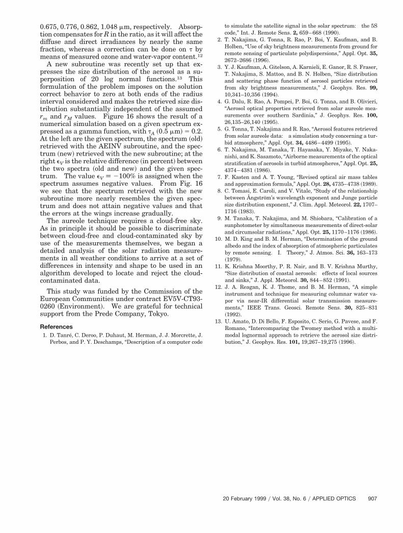
ssed as a histogram ~old! and as a set of log normals ~new!. Right,. Data are from a simulation.

xpretrum

swstt

Abudmdac

E0s

to simulate the satellite signal in the solar spectrum: the 5S
0.675, 0.776, 0.862, 1.048 mm, respectively. Absorp-tion compensates for R in the ratio, as it will affect thediffuse and direct irradiances by nearly the samefraction, whereas a correction can be done on t bymeans of measured ozone and water-vapor content.12
A new subroutine was recently set up that ex-presses the size distribution of the aerosol as a su-perposition of 20 log normal functions.13 Thisformulation of the problem imposes on the solutioncorrect behavior to zero at both ends of the radiusinterval considered and makes the retrieved size dis-tribution substantially independent of the assumedrm and rM values. Figure 16 shows the result of anumerical simulation based on a given spectrum ex-pressed as a gamma function, with tA ~0.5 mm! 5 0.2.At the left are the given spectrum, the spectrum ~old!retrieved with the AEINV subroutine, and the spec-trum ~new! retrieved with the new subroutine; at theright eV is the relative difference ~in percent! betweenthe two spectra ~old and new! and the given spec-trum. The value eV [ 2100% is assigned when thepectrum assumes negative values. From Fig. 16e see that the spectrum retrieved with the new

ubroutine more nearly resembles the given spec-rum and does not attain negative values and thathe errors at the wings increase gradually.

The aureole technique requires a cloud-free sky.s in principle it should be possible to discriminateetween cloud-free and cloud-contaminated sky byse of the measurements themselves, we began aetailed analysis of the solar radiation measure-ents in all weather conditions to arrive at a set of

ifferences in intensity and shape to be used in anlgorithm developed to locate and reject the cloud-ontaminated data.

This study was funded by the Commission of theuropean Communities under contract EV5V-CT93-260 ~Environment!. We are grateful for technicalupport from the Prede Company, Tokyo.

References1. D. Tanre, C. Deroo, P. Duhaut, M. Herman, J. J. Morcrette, J.

Perbos, and P. Y. Deschamps, “Description of a computer code

code,” Int. J. Remote Sens. 2, 659–668 ~1990!.2. T. Nakajima, G. Tonna, R. Rao, P. Boi, Y. Kaufman, and B.

Holben, “Use of sky brightness measurements from ground forremote sensing of particulate polydispersions,” Appl. Opt. 35,2672–2686 ~1996!.

3. Y. J. Kaufman, A. Gitelson, A. Karnieli, E. Ganor, R. S. Fraser,T. Nakajima, S. Mattoo, and B. N. Holben, “Size distributionand scattering phase function of aerosol particles retrievedfrom sky brightness measurements,” J. Geophys. Res. 99,10,341–10,356 ~1994!.

4. G. Dalu, R. Rao, A. Pompei, P. Boi, G. Tonna, and B. Olivieri,“Aerosol optical properties retrieved from solar aureole mea-surements over southern Sardinia,” J. Geophys. Res. 100,26,135–26,140 ~1995!.

5. G. Tonna, T. Nakajima and R. Rao, “Aerosol features retrievedfrom solar aureole data: a simulation study concerning a tur-bid atmosphere,” Appl. Opt. 34, 4486–4499 ~1995!.

6. T. Nakajima, M. Tanaka, T. Hayasaka, Y. Miyake, Y. Naka-nishi, and K. Sasamoto, “Airborne measurements of the opticalstratification of aerosols in turbid atmospheres,” Appl. Opt. 25,4374–4381 ~1986!.

7. F. Kasten and A. T. Young, “Revised optical air mass tablesand approximation formula,” Appl. Opt. 28, 4735–4738 ~1989!.

8. C. Tomasi, E. Caroli, and V. Vitale, “Study of the relationshipbetween Ångstrom’s wavelength exponent and Junge particlesize distribution exponent,” J. Clim. Appl. Meteorol. 22, 1707–1716 ~1983!.

9. M. Tanaka, T. Nakajima, and M. Shiobara, “Calibration of asunphotometer by simultaneous measurements of direct-solarand circumsolar radiations,” Appl. Opt. 25, 1170–1176 ~1986!.

10. M. D. King and B. M. Herman, “Determination of the groundalbedo and the index of absorption of atmospheric particulatesby remote sensing. I. Theory,” J. Atmos. Sci. 36, 163–173~1979!.

11. K. Krishna Moorthy, P. R. Nair, and B. V. Krishna Murthy,“Size distribution of coastal aerosols: effects of local sourcesand sinks,” J. Appl. Meteorol. 30, 844–852 ~1991!.

12. J. A. Reagan, K. J. Thome, and B. M. Herman, “A simpleinstrument and technique for measuring columnar water va-por via near-IR differential solar transmission measure-ments,” IEEE Trans. Geosci. Remote Sens. 30, 825–831~1992!.

13. U. Amato, D. Di Bello, F. Esposito, C. Serio, G. Pavese, and F.Romano, “Intercomparing the Twomey method with a multi-modal lognormal approach to retrieve the aerosol size distri-bution,” J. Geophys. Res. 101, 19,267–19,275 ~1996!.


calibration and data elaboration procedure for sky irradiance measurements

Documents