Temididiscussionedel Servizio Studi

Emu Fiscal Rules: is There a Gap?

by F. Balassone and D. Monacelli

Number 375 - July 2000

The purpose of the “Temi di discussione” series is to promote the circulation ofworkingpapers prepared within the Bank of Italy or presented in Bank seminars by outsideeconomists with the aim of stimulating comments and suggestions.

The views expressed in the articles are those of the authors and do not involve theresponsibility of the Bank.

Editorial Board:MASSIMO ROCCAS, FABRIZIO BALASSONE, GIUSEPPE PARIGI, DANIELE TERLIZZESE, PAOLOZAFFARONI; RAFFAELA BISCEGLIA (Editorial Assistant).

SINTESI

Il contenuto di questo lavoro esprime solamente le opinioni degli autori; pertanto

non rappresenta la posizione ufficiale della Banca d’Italia

Il Patto di stabilità e crescita del giugno del 1997 impegna i paesi dell’Unione europeaa raggiungere una posizione di bilancio prossima al pareggio o in avanzo nel medio termine.Questa integrazione alla regola stabilita nel Trattato di Maastricht, che prevede che idisavanzi non possano superare il tre per cento del PIL, se non in circostanze eccezionali,tende a conciliare la solidità delle finanze pubbliche con la disponibilità di margini adeguatiper la conduzione di politiche di stabilizzazione. Tuttavia, poiché la regola del Trattatorelativa al debito non è stata corrispondentemente integrata, esiste il rischio che talericonciliazione non sia completa. Per utilizzare il bilancio a fini di stabilizzazione,garantendo nel contempo la riduzione del rapporto tra debito e prodotto (come richiesto dalTrattato per valori di tale rapporto superiori al 60 per cento), può essere necessarioconseguire un elevato avanzo del saldo di bilancio corretto per il ciclo. Per tassi di crescitadel PIL positivi in termini nominali, l’avanzo richiesto cresce al diminuire del debito. I paesiche si prefiggano obiettivi di bilancio poco ambiziosi potrebbero trovarsi costretti adadottare politiche procicliche nelle fasi congiunturali meno favorevoli. L’interazione tra laregola relativa al disavanzo e quella relativa al debito è resa complessa dal fatto che ledefinizioni di tali variabili adottate nella Procedura dei disavanzi eccessivi non fannoriferimento allo stesso insieme di transazioni e alle stesse regole contabili.

EMU FISCAL RULES: IS THERE A GAP?

di Fabrizio Balassone* e Daniela Monacelli*

Abstract

The Stability and Growth Pact sets a medium-term target for fiscal policy of abudgetary position “close to balance or in surplus”. This addition to the deficit rule definedby the Maastricht Treaty has been interpreted as an attempt to reconcile the objective ofsound public finances with the availability of adequate margins for stabilisation. However,with the debt rule set in the Treaty unchanged, there is a risk that the Pact will not fullyachieve the desired reconciliation. Using the budget to implement stabilisation policy whilestill ensuring a reduction in the debt-to-GDP ratio during cyclical downturns, as required bythe Treaty, is likely to require large structural surpluses. Assuming positive nominal growthrates, the closer the debt ratio is to 60 per cent the larger are the surpluses needed. Ifcountries with debt ratios higher than 60 per cent set insufficiently ambitious deficit targets,they will not be able to make full use of the margins allowed by the 3 per cent threshold.During cyclical downturns such countries may have to adopt a pro-cyclical budgetary stance.The regulation of the interaction between deficit and debt rules is complicated by the EUdefinitions of debt and deficit, as they refer to different groups of transactions and are basedon different accounting conventions.

JEL Classification: E61, H6

Keywords: fiscal rules; stabilisation policy

Contents

1. Introduction.......................................................................................................................... 72. The fiscal rules in the Treaty: the actual budget constraint ................................................. 93. The risk of pro-cyclical fiscal policy ................................................................................. 124. The Stability and Growth Pact........................................................................................... 185. Possible solutions............................................................................................................... 23

5.1 Exceptions to the debt rule ......................................................................................... 245.2 The abolition of the debt rule and the adoption of a different deficit definition ........ 255.3 “Rainy-day funds” ...................................................................................................... 28

References……………………………………………………………………………………30

* Bank of Italy, Research Department.

1. Introduction1

According to the EMU fiscal rules laid down in the Treaty of Maastricht, the general

government deficit should not exceed 3 per cent of GDP and the ratio of general government

gross debt to GDP should be lower than 60 per cent or, if higher, diminishing “sufficiently”

and approaching that threshold “at a satisfactory pace”. The maximum deficit level

consistent with a diminishing debt ratio may be lower or higher than 3 per cent of GDP

depending on the debt level and the GDP growth rate. The objective of the rules was to

ensure that the fiscal behaviour of prospective EMU members was sound2.

As the initial deficit and debt ratios differed widely among the EU countries, so did the

effort demanded to achieve convergence towards the thresholds set in the Treaty.

Accordingly, the fact that the interaction between the deficit and debt rules implied different

constraints depending on the debt level and the GDP growth rate was not deemed to be a

problem.

Monetary policy is no longer available to individual EMU countries as a counter-

cyclical instrument. As regards use of the budget as a stabilisation tool, the Treaty allows a

deficit higher than 3 per cent of GDP during severe recessions. No exceptions are made to

the debt rule, the application of which may result in the budget having a pro-cyclical stance.

In general, the Treaty leaves it up to member states to make sure that compliance with the

EMU fiscal rules is consistent with any other target they assign to budgetary policy3.

1 We wish to thank Marco Buti, Daniele Franco and Stefania Zotteri for helpful comments. The views

expressed in the article are those of the authors and do not involve the responsibility of the Bank of Italy.E-mail: balassone.fabrizio@insedia.interbusiness.it and monacelli.daniela@insedia.interbusiness.it

2 The Treaty refers to the ratio of gross debt to GDP and requires it to be decreasing. We do not tackle theissue of whether this is an appropriate measure for assessing fiscal sustainability. For a discussion of theeconomic rationale of the EMU fiscal rules, see Eichengreen and Von Hagen (1996). For a discussion of theconditions for fiscal sustainability, see Balassone and Franco (2000a).

3 For an overview of the role of fiscal policy in the EMU, see European Commission (1997).

8

The Stability and Growth Pact makes the link between fiscal rules and stabilisation

policy explicit. It is intended to provide a self-disciplinary mechanism serving to reconcile

sound fiscal stances with adequate margins for counter-cyclical policies4.

To this end, the Pact supplements the deficit rule by introducing a medium-term target

of a position “close to balance or in surplus”. The Ecofin Council subsequently clarified that

the target was to be achieved “over the cycle”; in other words it can be interpreted as

applying to structural balances, i.e. balances net of cyclical effects5.

The debt rule was not similarly supplemented by the Stability and Growth Pact.

In this paper we argue that, with the debt rule unchanged, the innovation introduced by

the Pact may not be sufficient to avoid the risk that the EMU fiscal rules will call for pro-

cyclical policies. Even if they run a balanced structural budget, countries with debt-to-GDP

ratios greater than or close to 60 per cent will not be able to make full use of the margin

allowed by the 3 per cent threshold if they have to comply with the debt rule. Moreover, the

debt rule can be shown to produce tighter constraints for countries which are closer to the 60

per cent threshold than for those which are further away from it.

We also argue that there are three ways to make the EMU rules fully consistent with

the double target of flexibility and soundness in fiscal stances: a) exceptions to the debt rule

can be explicitly allowed while leaving the deficit rule unaltered; b) the debt rule can be

abolished and the deficit rule applied to a different definition of budget balance, closer to the

first difference in gross debt; c) “rainy-day funds” can be introduced to protect against the

effects of the cycle on the debt ratio.

The structure of the paper is as follows: the next section shows how the Treaty’s deficit

and debt rules interact; section 3 analyses the implications for stabilisation policies; section 4

extends the argument to the changes introduced by the Stability and Growth Pact; section 5

concludes by discussing possible solutions.

4 On the targets and the interpretation of the Stability and Growth Pact, see Artis and Winkler (1997),

Buti et al. (1997; 1998), Eichengreen and Wyplosz (1998).5 This interpretation finds support in Council Resolution of 16-17 June 1997, in Council Regulation of 7

July 1997 No. 1466/97, in the Opinion of the Monetary Committee of 12 October 1998 endorsed by theCouncil.

9

2. The fiscal rules in the Treaty: the actual budget constraint

The dynamics of the debt-to-GDP ratio (d) can be approximated by:

(1) dt = [1/(1+gt )] dt-1 + bt

where gt is the nominal growth rate of GDP and bt is the budget balance (bt>0

indicates a deficit)6.

The Treaty rules can be expressed as follows:

(2) deficit rule bt ≤ 3.0

(3a) debt rule dt ≤ 60 for d t-1 ≤ 60

(3b) ∆dt < 0 for d t-1 > 60

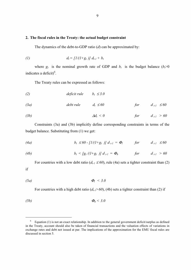
Constraints (3a) and (3b) implicitly define corresponding constraints in terms of the

budget balance. Substituting from (1) we get:

(4a) bt ≤ 60 - [1/(1+gt )] d t-1 = Φl for d t-1 ≤ 60

(4b) bt < [gt /(1+gt )] d t-1 = Φh for d t-1 > 60

For countries with a low debt ratio (dt-1 ≤ 60), rule (4a) sets a tighter constraint than (2)

if

(5a) Φl < 3.0

For countries with a high debt ratio (dt-1>60), (4b) sets a tighter constraint than (2) if

(5b) Φh < 3.0

6 Equation (1) is not an exact relationship. In addition to the general government deficit/surplus as defined

in the Treaty, account should also be taken of financial transactions and the valuation effects of variations inexchange rates and debt not issued at par. The implications of the approximation for the EMU fiscal rules arediscussed in section 5.

10

For given values of gt and dt-1, Φl and Φh define the maximum deficit level consistent

with debt constraints (3a) and (3b). Equations (5a) and (5b) define the set of combinations

[gt , dt-1 ] for which a deficit ratio lower than 3 per cent is required in order, respectively, to

prevent the debt ratio from exceeding the 60 per cent threshold and ensure that it decreases.

The budget constraint for each country thus does not depend only on whether the debt

ratio is above or below 60 per cent but is also affected by the ratio’s actual value and by the

nominal GDP growth rate.

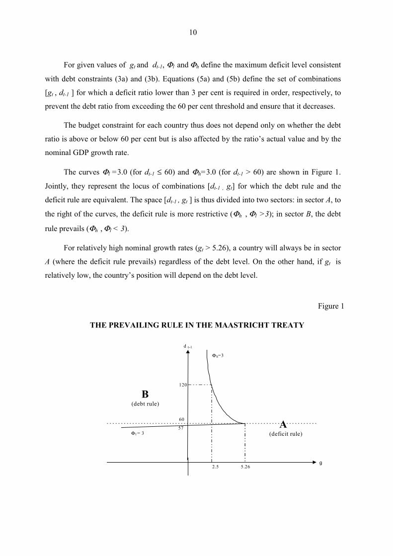
The curves Φl =3.0 (for dt-1 ≤ 60) and Φh=3.0 (for dt-1 > 60) are shown in Figure 1.

Jointly, they represent the locus of combinations [dt-1 , gt] for which the debt rule and the

deficit rule are equivalent. The space [dt-1 , gt ] is thus divided into two sectors: in sector A, to

the right of the curves, the deficit rule is more restrictive (Φh , Φl >3); in sector B, the debt

rule prevails (Φh , Φl < 3).

For relatively high nominal growth rates (gt > 5.26), a country will always be in sector

A (where the deficit rule prevails) regardless of the debt level. On the other hand, if gt is

relatively low, the country’s position will depend on the debt level.

60

d t-1

g5.26

57

120

2.5

B(debt rule)

A(deficit rule)

Φh=3

Φ l = 3

Figure 1

THE PREVAILING RULE IN THE MAASTRICHT TREATY

11

Given the shape of the Φ=curves, countries with a debt ratio close to 60 per cent may

fall in sector B (where the debt rule prevails and the maximum deficit allowed is lower than

3 per cent of GDP) even if gt is just below 5.26 per cent. As dt moves further away from the

60 per cent threshold, the nominal growth rate below which a country falls in sector B

decreases.

In other words, the range of debt ratios over which the debt rule prevails widens as the

growth rate decreases: approximately, if g≅4 the debt rule prevails for 59<dt-1<78 per cent; if

g≅1 the debt rule prevails for 58<dt-1<300 per cent. The widening is not symmetric: it is

extremely unlikely for the debt rule to prevail for countries whose debt ratio is well below 60

per cent (for dt-1≅55, g ≤-3 would be needed). Table 1 gives examples of the values of Φh

and Φl for different values of the debt ratio and the GDP growth rate (equations 4a and 4b).

The figures in bold correspond to the cases in which the debt rule prevails (the values are

lower than 3 per cent). Perversely, for high-debt countries with positive growth rates, the

lower the debt ratio the tighter the budget constraint imposed by the debt rule7.

7 This point has been made by several authors; see e.g. Pasinetti (1997).

Table 1

THE PREVAILING RULE FOR GIVEN DEBT AND GDP GROWTH VALUES

H ig h d e b t c o u n tr ie s ( v a lu e s o f

ΦΦΦΦ

h

)g d

6 5 7 0 8 0 9 0 1 0 0 1 1 0 1 2 0 1 3 0 1 4 0 1 5 0 1 6 0

- 4

- 2 .7 - 2 .9 - 3 .3 - 3 .8 - 4 .2 - 4 .6 - 5 .0 - 5 .4 - 5 .8 - 6 .3 - 6 .7

- 2

- 1 .3 - 1 .4 - 1 .6 - 1 .8 - 2 .0 - 2 .2 - 2 .4 - 2 .7 - 2 .9 - 3 .1 - 3 .3

0

0 .0 0 .0 0 .0 0 .0 0 .0 0 .0 0 .0 0 .0 0 .0 0 .0 0 .0

2

1 .3 1 .4 1 .6 1 .8 2 .0 2 .2 2 .4 2 .5 2 .7 2 .9 3 .1

4

2 .5 2 .7 3 .1 3 .5 3 .8 4 .2 4 .6 5 .0 5 .4 5 .8 6 .2

L o w d e b t c o u n tr ie s ( v a lu e s o f

ΦΦΦΦ

l

)

g d

1 0 1 5 2 0 2 5 3 0 3 5 4 0 4 5 5 0 5 5 6 0

- 4

4 9 .6 4 4 .4 3 9 .2 3 4 .0 2 8 .8 2 3 .5 1 8 .3 1 3 .1 7 .9 2 .7 - 2 .5

- 2

4 9 .8 4 4 .7 3 9 .6 3 4 .5 2 9 .4 2 4 .3 1 9 .2 1 4 .1 9 .0 3 .9 - 1 .2

0

5 0 .0 4 5 .0 4 0 .0 3 5 .0 3 0 .0 2 5 .0 2 0 .0 1 5 .0 1 0 .0 5 .0 0 .0

2

5 0 .2 4 5 .3 4 0 .4 3 5 .5 3 0 .6 2 5 .7 2 0 .8 1 5 .9 1 1 .0 6 .1 1 .2

4

5 0 .4 4 5 .6 4 0 .8 3 6 .0 3 1 .2 2 6 .3 2 1 .5 1 6 .7 1 1 .9 7 .1 2 .3

12

3. The risk of pro-cyclical fiscal policy

The Treaty leaves it up to each member country to ensure that compliance with the

EMU fiscal rules is consistent with any other target assigned to budgetary policy.

If a country wants to avoid being forced to adopt a pro-cyclical stance during

unfavourable cyclical phases, it is its own responsibility to evaluate the budget response to

cyclical developments and choose a structural balance sufficiently below the 3 per cent

threshold.

The Treaty foresees exceptions to the deficit rule only in the event of severe recessions

and provided that the deficit remains close to the threshold and exceeds it for a limited

period only8 (see Box 1). However, the absence of exceptions to the debt rule can still

Box 1: Flexibility in the EMU fiscal rules

Article 104C(2a) of the Treaty states that the deficit-to-GDP ratio should not exceed “a referencevalue, unless: either the ratio has declined substantially and continuously and reached a level thatcomes close to the reference value; or, alternatively, the excess over the reference value is onlyexceptional and temporary and the ratio remains close to the reference value”.Article 104C(2b) states that the debt-to-GDP ratio should not exceed “a reference value, unless theratio is sufficiently diminishing and approaching the reference value at a satisfactory pace”.The Protocol on excessive deficits sets the reference values at, respectively, 3 and 60 per cent.The Stability and Growth Pact has subsequently made clear that the excess over the referencevalue concerning the deficit is deemed exceptional, and thus in line with EU rules, if it derives froma severe recession causing a reduction in real GDP of at least 2 per cent (the Council can extendthe definition to reductions in GDP of at least 0.75 per cent).This exception only applies to a breach of the 3 per cent threshold (not to an interruption of thetrend reduction required for deficits already above 3 per cent); it does not apply to the debt rule.It can be argued that while the Treaty explicitly adds a continuity clause for deficit reduction, itdoes not do so for debt reduction, so that EU rules do not always require a reduction in the debtratio. However, if this is the case, there would still be a problem of interpretation:

a) when is an increase in debt allowed?b) the debt rule requires the debt to be “sufficiently diminishing and approaching the

reference value”, which seems to imply a continuous process; the need for high-debtcountries to achieve a steady decline in their debt ratio has been often highlighted.

8 The three conditions make the 3 per cent threshold extremely binding (see Buti et al., 1997).

13

make pro-cyclical action necessary: a country where the debt rule prevails may be forced to

take pro-cyclical action even when a recession qualifies as severe, notwithstanding the

efforts made to build up adequate margins for the deficit rule.

To analyse the implications of the “Maastricht rules” for stabilisation policy, the deficit

ratio can be split into its “structural” (bs) and “cyclical” (bc) components. Given the inflation

rate (π), the first component is the value the deficit would have if real GDP growth (γ) were

at its trend value (γs). The second component is the effect of cyclical fluctuations on the

budget, given by the product of the output gap (defined here as the difference between the

trend and actual real GDP growth rates: γ=s-γ=t ) 9 and the elasticity of the budget with respect

to GDP (η):

(6) bt = bs + bc = bs + (γ=s - γ=t ) η

Defining gs =γ=s + π=t , and taking into account that gt = γ=t +π=t 10, (6) can also be

written using nominal rates as:

(6’) bt = bs + (gs - gt ) η

The deficit ratio equals its structural component when real GDP growth is at its trend

value (γs -γt =0); it is higher than the structural component when γ=s>γ=t (i.e. in unfavourable

cyclical phases); it is lower than the structural component when γ=s<γ=t (in favourable

cyclical phases).

Substituting (6) into (2) gives:

(7) bs ≤ 3.0 - (γ=s - γ=t ) η

If this condition is met by a narrow margin when growth is at its trend value , i.e. if

bs ≅ 3.0, it may be necessary to reduce bs in order to make room for the increase in the

cyclical component of the deficit during a cyclical downturn. In other words, pro-cyclical

14

measures may be called for during recessions. In general, (7) shows that this occurs

whenever a worsening of the deficit induced by the cycle, as given by (γ=s - γ=t )η, is larger

than the difference between the 3 per cent threshold and the structural balance.

A similar problem arises with the debt rule. Substituting (6) into (4a) and (4b) gives:

(8a) bs ≤ 60 - [1/(1+gt )] d t-1 - (γ=s - γ=t ) η for d t-1 ≤ 60

(8b) bs < [gt /(1+gt )] d t-1 - (γ=s - γ=t ) η for d t-1 > 60

If these constraints are met by a narrow margin when growth is at its trend value, i.e.

if bs ≅ 60-[1/(1+gs)]dt-1 and bs ≅ [gs/(1+gs )]dt-1 respectively, it may be necessary to reduce

bs during downturns.

The need for pro-cyclical action will depend not only on the effect of the cycle on the

budget, but also on the effect of the cycle on the debt ratio.

In the case of low-debt countries, (8a) shows that pro-cyclical action is necessary if the

cyclical effect on the budget determines an actual deficit, bt=bs+(γs-γt )η, higher than the

difference between the 60 per cent threshold and the debt-to-GDP ratio that would be

reached due to the cyclical effect alone, i.e. 60-[1/(1+gt )]dt-1.

For high-debt countries, (8b) shows that pro-cyclical action is necessary if the cyclical

effect on the budget determines an actual deficit higher than the change in the debt ratio

determined by the cycle alone, i.e. [gt /(1+gt )]dt-1. It should be noted that the cyclical effect

on the debt ratio decreases as dt-1 decreases, so that, for given positive growth rates,

countries whose debt ratio is closer to the 60 per cent threshold are more at risk.

Constraints (7) and (8) are binding under different circumstances. Starting from a

condition of compliance with the “Maastricht rules”, a country may have to take pro-cyclical

9 Note that this is different from the usual definition of the output gap, which is the difference between

actual and trend (or potential) GDP as a percentage of the latter. The two definitions are essentially equivalentunder the assumption that GDP at time t-1 is at its trend value. The definition adopted here simplifies thealgebra without affecting the qualitative results of the analysis.

10 To keep things simple, we leave out the second-order term γπ.

15

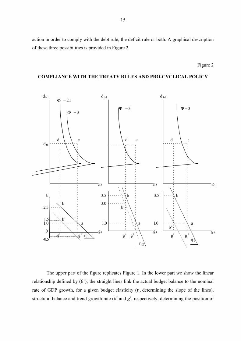
action in order to comply with the debt rule, the deficit rule or both. A graphical description

of these three possibilities is provided in Figure 2.

Figure 2

COMPLIANCE WITH THE TREATY RULES AND PRO-CYCLICAL POLICY

Φ = 2.5

Φ = 3

dt-1

bt

g t

g tη=1

1.0

2.5

a

b

d d

g’

d 0

0

b’

3.5

1.0

Φ = 3

dt-1

cc

a

b

g t

g t

3.0

d t-1

g t

g t

a

b3.5

cd

Φ = 3

1.0

b’

b’

η=2

1.5

-0.5g s g s g s

η=3g’ g’

The upper part of the figure replicates Figure 1. In the lower part we show the linear

relationship defined by (6’); the straight lines link the actual budget balance to the nominal

rate of GDP growth, for a given budget elasticity (η,=determining the slope of the lines),

structural balance and trend growth rate (bs and gs, respectively, determining the position of

16

the lines in the [b, g] space). The structural balance corresponding to each line is equal to the

value of bt along that line for gt=gs : for the solid lines, for example, the corresponding

structural deficit is equal to 1.0 per cent.

Points a (in the lower part) and c (in the upper part) describe a high-debt country

where growth is at its trend value, (gt=gs), the structural deficit is equal to 1.0 per cent of

GDP and the debt ratio is d0 . As c lies to the right of the curve Φ=3, for such a country the

deficit rule prevails.

Assuming a cyclical downturn causing the nominal growth rate to fall from gs to g’, in

the graph on the left the country moves from a to b and the deficit grows from 1.0 to 2.5 per

cent, staying below the 3 per cent threshold. The move from a to b in the lower part of the

figure corresponds to a move from c to d in the upper part: the country moves to the left of

Φ=3, where the debt rule prevails: as d is also to the left of Φ=2.5, compliance with the debt

rule calls for a deficit lower than 2.5 per cent of GDP. The actual deficit reduction the

country is required to achieve implies the adoption of pro-cyclical discretionary measures to

reduce the structural deficit. Assuming that the deficit needed for debt rule compliance at

point d is 1.5 per cent, the country would have to move to the dotted line in the lower part of

the graph, from b to b’, where the structural balance records a 0.5 per cent surplus.

The graph in the middle assumes a smaller reduction in the growth rate and a higher

budget elasticity (η2>η1). The country does not move into the sector where the debt rule

prevails, but the actual deficit exceeds the 3.0 per cent threshold. In this case, discretionary

pro-cyclical measures are only needed to comply with the deficit rule.

Lastly, the graph on the right-hand side shows the case in which the reductions in the

growth rate and the budget elasticity cause both rules to be breached: point d is to the left of

Φ=3 and b implies an actual deficit exceeding the 3.0 per cent limit.

Tables 2 and 3 give some numerical examples of the working of the deficit and debt

rule respectively, and show the cases in which the debt rule is tighter than the deficit rule.

In both tables we assume a structural deficit equal to 1.0 per cent of GDP; a trend

growth rate of real GDP of 2.5 per cent and a budget elasticity of 0.5 (the two latter

assumptions are in line with the European Commission’s estimates for EU countries in

17

Table 2

PRO-CYCLICAL MEASURES AND THE DEFICIT RULE

E f f e c t o f t h e N e e d f o r

b s γγγγ s γγγγ t ηηηη =

==

=

c y c l e o n p r o - c y c l i c a lt h e b u d g e t m e a s u r e s

( γ s- γ t

) η 3 . 0 - b s

( 7 ) b s < = 3 . 0 - ( γ s - γ t ) η

1 2 . 5 - 4 0 . 5 3 . 2 5 2 y e s1 2 . 5 - 3 . 5 0 . 5 3 2 y e s1 2 . 5 - 3 0 . 5 2 . 7 5 2 y e s1 2 . 5 - 2 . 5 0 . 5 2 . 5 2 y e s1 2 . 5 - 2 0 . 5 2 . 2 5 2 y e s1 2 . 5 - 1 . 5 0 . 5 2 2 n o1 2 . 5 - 1 0 . 5 1 . 7 5 2 n o1 2 . 5 - 0 . 5 0 . 5 1 . 5 2 n o1 2 . 5 0 0 . 5 1 . 2 5 2 n o1 2 . 5 0 . 5 0 . 5 1 2 n o

Table 3

PRO-CYCLICAL MEASURES AND THE DEBT RULE (ππππ=1.5)

Effect of the Effect of the Need forb s γγγγs γγγγt ηηηη ==== d t-1 cycle on cycle on Correction pro-cyclical

the budget the debt action(a)=b s +( γs -γt ) η (b)=[g t /(1+g t)]d t-1 (a) - (b)

(8b) b s <[g t /(1+g t)]d t-1 - ( γs - γt ) η

1 2.5 0 0.5 120 2.25 1.77 0.48 yes1 2.5 0 0.5 110 2.25 1.63 0.62 yes1 2.5 0 0.5 100 2.25 1.48 0.77 yes1 2.5 0 0.5 90 2.25 1.33 0.92 yes1 2.5 0 0.5 80 2.25 1.18 1.07 yes1 2.5 0 0.5 70 2.25 1.03 1.22 yes

Effect of the Effect of the Need forb s γγγγs γγγγt ηηηη d t-1 cycle on cycle on Correction pro-cyclical

the budget the debt needed actionl(a) = b s +( γs -γt ) η (b)=60-[1/(1+g t )]dt-1 (a) - (b)

(8a) b s <=60-[1/(1+g t )]d t-1 - (γs - γt ) η

1 2.5 0 0.5 60 2.25 0.89 1.36 yes1 2.5 0 0.5 50 2.25 10.74 -8.49 no1 2.5 0 0.5 40 2.25 20.59 -18.29 no1 2.5 0 0.5 30 2.25 30.44 -28.19 no

needed

18

1998). In order to compute the dynamics of the debt ratio, in Table 3 an inflation rate of 1.5

per cent is assumed, in line with ECB’s institutional target.

As regards the deficit rule (Table 2), pro-cyclical action is only necessary for relatively

large output gaps (more than 4 percentage points11); moreover, most of these cases would

qualify for the exception allowed by the Treaty as γt≤-2. As for the debt rule (Table 3), an

output gap of 2.5 points is sufficient to trigger pro-cyclical action for debt ratios exceeding

the 60 per cent threshold or close to it. The size of the necessary correction may be

substantial: it ranges from 0.5 per cent of GDP for a 120 per cent debt ratio to 1.4 per cent

for a 60 per cent ratio.

4. The Stability and Growth Pact

By adopting the Stability and Growth Pact, the EU member states have introduced a

self-disciplinary mechanism which obliges them to build up margins for stabilisation.

The Pact sets a medium-term target of a budget position “close to balance or in

surplus”. According to the Ecofin Council’s subsequent interpretation, this target is to be met

“over the cycle”. The Pact’s provisions can thus be interpreted as imposing a ceiling on

structural deficits and setting it far enough from the 3 per cent threshold (which continues to

apply to actual deficits) to reduce the risk that pro-cyclical action will be needed to avoid

breaching the deficit rule during downturns.12 In Figure 2 the Pact’s provisions correspond to

imposing a constraint on the position of the straight lines in the lower part of the graphs: they

must cross the horizontal axis where growth is at its trend value (g=gs) or to the left of that

point.

However, since the debt rule has not been changed, the Pact has no effect in situations

where the debt rule prevails.

In Figure 3, the situation of a country with a balanced structural budget is examined

(bt=0 when gt =gs). The figure assumes an inflation rate of 1.5 per cent and a trend growth

11 According to European Commission estimates, the average of the maximum output gaps recorded in EU

countries between 1960 and 1997 is 4 percentage points (see Buti et al., 1997).12 See Buti et al. (1997) for some simulations based on historical data.

19

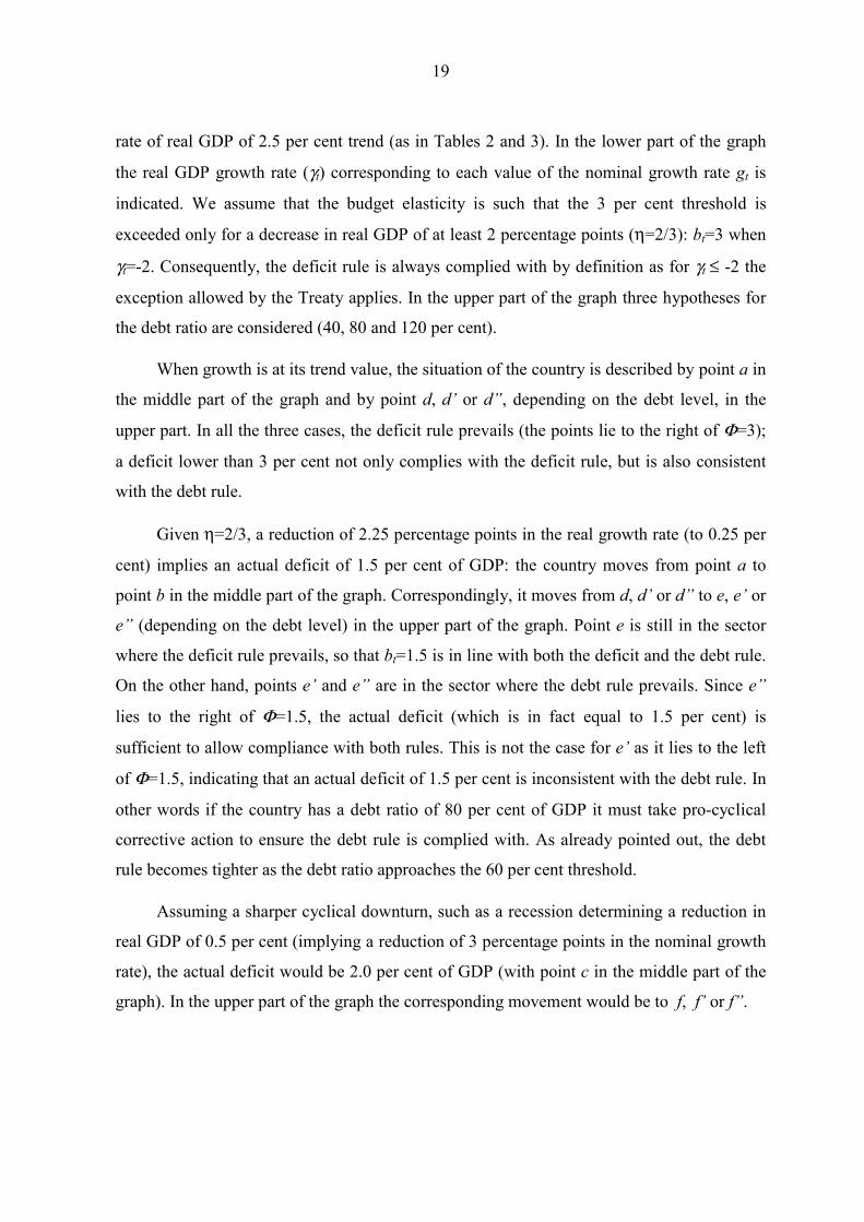
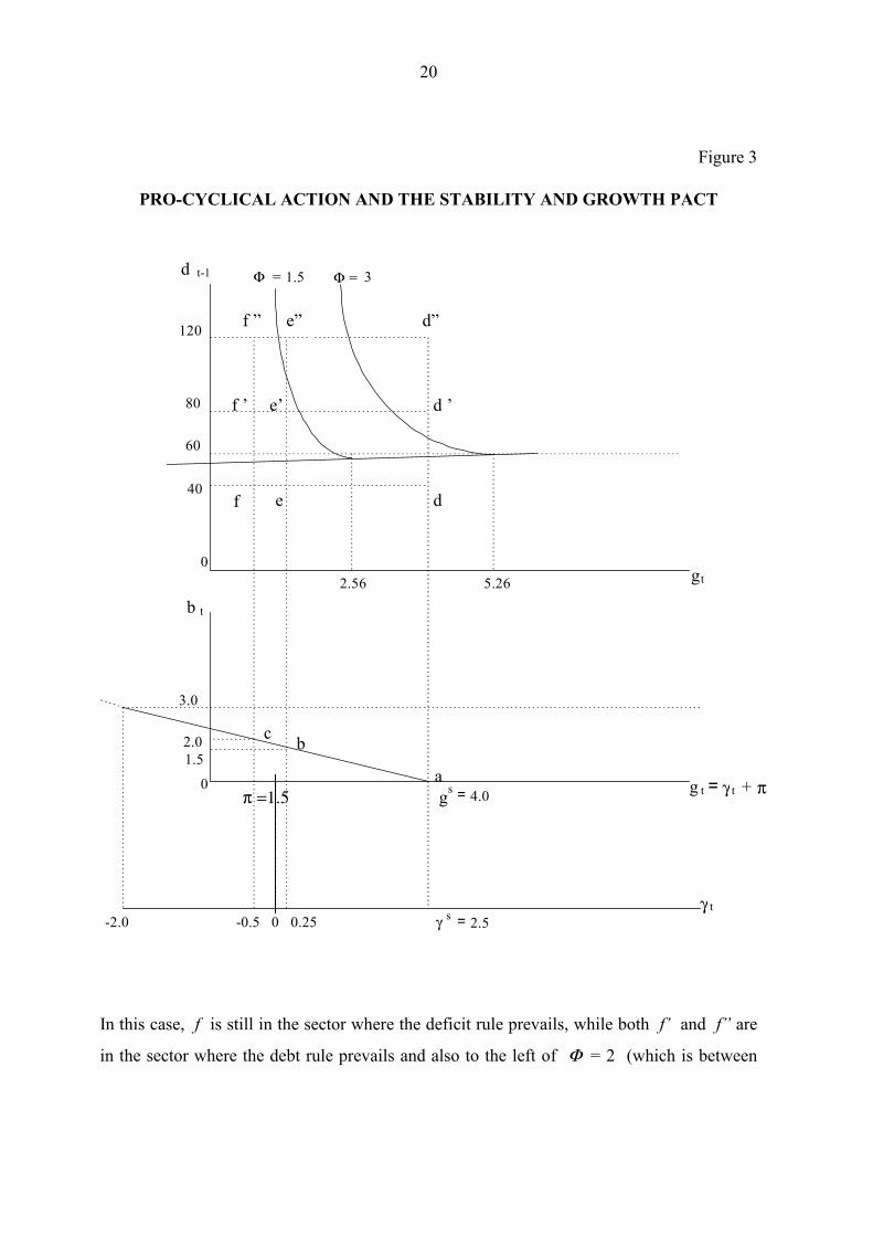
rate of real GDP of 2.5 per cent trend (as in Tables 2 and 3). In the lower part of the graph

the real GDP growth rate (γt) corresponding to each value of the nominal growth rate gt is

indicated. We assume that the budget elasticity is such that the 3 per cent threshold is

exceeded only for a decrease in real GDP of at least 2 percentage points (η=2/3): bt=3 when

γt=-2. Consequently, the deficit rule is always complied with by definition as for γt ≤ -2 the

exception allowed by the Treaty applies. In the upper part of the graph three hypotheses for

the debt ratio are considered (40, 80 and 120 per cent).

When growth is at its trend value, the situation of the country is described by point a in

the middle part of the graph and by point d, d’ or d”, depending on the debt level, in the

upper part. In all the three cases, the deficit rule prevails (the points lie to the right of Φ=3);

a deficit lower than 3 per cent not only complies with the deficit rule, but is also consistent

with the debt rule.

Given η=2/3, a reduction of 2.25 percentage points in the real growth rate (to 0.25 per

cent) implies an actual deficit of 1.5 per cent of GDP: the country moves from point a to

point b in the middle part of the graph. Correspondingly, it moves from d, d’ or d” to e, e’ or

e” (depending on the debt level) in the upper part of the graph. Point e is still in the sector

where the deficit rule prevails, so that bt=1.5 is in line with both the deficit and the debt rule.

On the other hand, points e’ and e” are in the sector where the debt rule prevails. Since e”

lies to the right of Φ=1.5, the actual deficit (which is in fact equal to 1.5 per cent) is

sufficient to allow compliance with both rules. This is not the case for e’ as it lies to the left

of Φ=1.5, indicating that an actual deficit of 1.5 per cent is inconsistent with the debt rule. In

other words if the country has a debt ratio of 80 per cent of GDP it must take pro-cyclical

corrective action to ensure the debt rule is complied with. As already pointed out, the debt

rule becomes tighter as the debt ratio approaches the 60 per cent threshold.

Assuming a sharper cyclical downturn, such as a recession determining a reduction in

real GDP of 0.5 per cent (implying a reduction of 3 percentage points in the nominal growth

rate), the actual deficit would be 2.0 per cent of GDP (with point c in the middle part of the

graph). In the upper part of the graph the corresponding movement would be to f, f’ or f”.

20

Figure 3

PRO-CYCLICAL ACTION AND THE STABILITY AND GROWTH PACT

d t-1

gt

60

Φ=== 1.5 Φ== 3

5.26

g t = γ t + π

3.0

γ t

π==1.5

-0.5 0 0.25 -2.0

�gs = 4.0

==γ s = 2.5

80

120

2.0 1.5

a

b c

d

d ’

d”

e

e’

e”

f

f ’

f ”

40

2.56 b t

0

0

In this case, f is still in the sector where the deficit rule prevails, while both f’ and f” are

in the sector where the debt rule prevails and also to the left of Φ=== 2 (which is between

21

Φ=== 1.5 and Φ== 3.0). In this case compliance with the debt rule requires pro-cyclical

action both when the debt ratio is 80 per cent and when it is 120 per cent.

The situation described in Figure 3 assumes a balanced structural budget. It can easily

be shown that even relatively high structural surpluses13 are not a sufficient condition to

avoid the risk that compliance with the debt rule will call for the adoption of pro-cyclical

measures. Higher (lower) budget elasticities would, ceteris paribus, worsen (better) the

situation as they would determine higher (lower) actual deficits14.

In conclusion, only countries with debt ratios well below 60 per cent can take full

advantage of the flexibility allowed by the 3 per cent threshold for the actual deficit: unless

an extraordinary reduction in real GDP growth occurs, these countries will never be in a

situation where the debt rule prevails. Countries with a debt ratio only just below 60 per cent

may find themselves to the left of the Φ curve even during non-severe recessions: for dt<60,

the slope of Φ, although small, is positive. The same applies to high debt countries. As noted

earlier, where growth rates are positive, deficit values consistent with a stable debt ratio

decrease as the ratio decreases, so that the scope for stabilisation policies decreases as the

debt ratio approaches the 60 per cent threshold.

In order to evaluate the potential relevance of the problem, Table 4 shows some

numerical simulations for EU countries. We assume a balanced structural budget, an

inflation rate of 1.5 per cent and two alternative hypotheses for real growth: in case (1) the

rate is set to zero; in case (2) each country’s worse result in the 1970-1998 period is used.

The computations are based on 1998 debt ratios (ESA79 figures) and the European

Commission’s estimates of trend growth rates and budget elasticities.

In case (1), γt=0, the debt rule would not be met by Sweden, the Netherlands, Spain,

Austria or Germany (∆dt>0, in bold in the table), that is high debt countries not too far away

from the 60 per cent threshold. Ireland, while complying with the debt rule, would breach the

deficit threshold (bt>3.0).

13 Whether a permanently restrictive fiscal stance is desirable is an entirely different issue which we do not

tackle here.14 With higher budget elasticities the risk of breaching the deficit rule increases as well.

22

Table 4

THE EFFECT OF POSITIVE OUTPUT GAPS ON THE DEBT-TO-GDP RATIOCase (1) Case (2)

High-debt countries π d t-1 η γ s γ t b t ∆d t γt b t ∆d t

Italy 1.5 118.7 0.5 1.7 0.0 0.9 -0.9 -2.1 1.9 2.6 Belgium 1.5 117.3 0.6 2.2 0.0 1.3 -0.4 -1.5 2.2 2.2 Greece 1.5 106.1 0.4 2.6 0.0 1.0 -0.5 -3.6 2.5 4.8 Sweden 1.5 73.1 0.9 2.1 0.0 1.9 0.8 -2.2 3.9 4.4 Netherlands 1.5 67.7 0.8 3.0 0.0 2.4 1.4 -1.2 3.4 3.2 Spain 1.5 65.6 0.6 3.0 0.0 1.8 0.8 -1.2 2.5 2.3 Austria 1.5 63.3 0.5 2.6 0.0 1.3 0.4 -0.4 1.5 0.8 Germany 1.5 61.1 0.5 2.2 0.0 1.1 0.2 -1.3 1.8 1.6Low-debt countries d t d t

France 1.5 58.5 0.5 2.2 0.0 1.1 58.7 -1.3 1.8 60.1 Denmark 1.5 58.1 0.7 2.5 0.0 1.8 59.0 -0.9 2.4 60.1 Portugal 1.5 57.8 0.5 3.2 0.0 1.6 58.5 -4.3 3.8 63.2 Ireland 1.5 52.1 0.5 8.9 0.0 4.5 55.8 -0.2 4.6 56.0 UK 1.5 49.4 0.6 2.3 0.0 1.4 50.0 -2.0 2.6 52.2 Finland 1.5 49.1 0.6 3.2 0.0 1.9 50.3 -7.1 6.2 58.2

In case (2), none of the countries with a debt ratio above 60 per cent would comply

with the debt rule (∆dt>0); the Netherlands and Sweden would also breach the deficit

threshold (bt>3.0), although Sweden would qualify for an exception (γt <-2.0)15. Among the

low-debt countries, France, Denmark and Portugal, i.e. the countries whose debt ratio is

closest to 60 per cent, would not comply with the debt rule (dt>60). Portugal would not

comply with the deficit rule either but, as in the case of Sweden, the exception would apply.

Ireland and Finland would comply with the debt rule but not with the deficit rule; only

Finland would qualify for an exception.

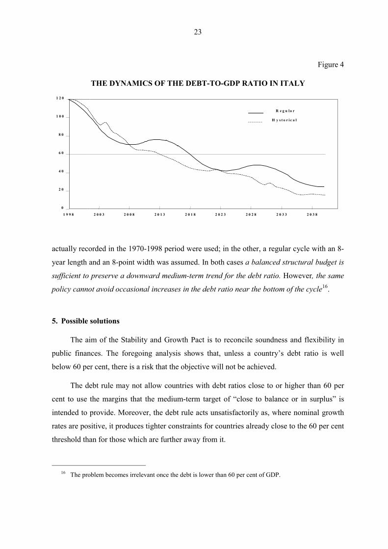
Finally, Figure 4 gives the results of two simulations run for Italy. Both are based upon

the debt ratio (ESA79 figures) recorded in 1998, a balanced structural budget, an inflation

rate of 1.5 per cent and the European Commission’s estimates of trend growth (1.7 per cent)

15 Note that γt <-2,0 for Italy and Greece as well, but this is not relevant to the debt rule.

23

Figure 4

THE DYNAMICS OF THE DEBT-TO-GDP RATIO IN ITALY

0

2 0

4 0

6 0

8 0

1 0 0

1 2 0

1 9 9 8 2 0 0 3 2 0 0 8 2 0 1 3 2 0 1 8 2 0 2 3 2 0 2 8 2 0 3 3 2 0 3 8

R e g u la r

H y s t o r i c a l

actually recorded in the 1970-1998 period were used; in the other, a regular cycle with an 8-

year length and an 8-point width was assumed. In both cases a balanced structural budget is

sufficient to preserve a downward medium-term trend for the debt ratio. However, the same

policy cannot avoid occasional increases in the debt ratio near the bottom of the cycle16.

5. Possible solutions

The aim of the Stability and Growth Pact is to reconcile soundness and flexibility in

public finances. The foregoing analysis shows that, unless a country’s debt ratio is well

below 60 per cent, there is a risk that the objective will not be achieved.

The debt rule may not allow countries with debt ratios close to or higher than 60 per

cent to use the margins that the medium-term target of “close to balance or in surplus” is

intended to provide. Moreover, the debt rule acts unsatisfactorily as, where nominal growth

rates are positive, it produces tighter constraints for countries already close to the 60 per cent

threshold than for those which are further away from it.

16 The problem becomes irrelevant once the debt is lower than 60 per cent of GDP.

24

Does this call for a modification of the EMU fiscal rules? If so, what changes can be

envisaged?

Three possible solutions can be examined: a) the explicit provision of exceptions to the

debt rule in connection with cyclical downturns; b) the outright abolition of the debt rule and

the application of the deficit rule to a different definition of the budget balance, closer to the

first difference in gross debt; c) the accumulation of financial assets to be used to buy back

debt during cyclical downturns (“rainy-day funds”). While the first two solutions imply the

acceptance of occasional increases in the debt ratios, the third aims at avoiding this. A full

analysis of the pros and cons of each option is beyond the scope of this paper. In what

follows only the main issues are explored. Each of the three solutions has its shortcomings;

perhaps the first one is easier to implement both technically and politically: it does not

require a major amendment of the present rules or any change in budgetary and debt

management practices.

5.1 Exceptions to the debt rule

As shown by the numerical simulations carried out for Italy, interruptions in the

process of reduction in the debt ratio due to higher deficits in low-growth phases would only

last for short periods and would have a relatively small effect if the structural balance is kept

close to balance or in surplus.

It thus follows that a sensible implementation of the rules should not call for the

declaration of an “excessive deficit” when an occasional increase in the debt-to-GDP ratio

occurs exclusively as a result of cyclical factors.

Indeed, some flexibility seems to be allowed: in 1997 Germany’s debt-to-GDP ratio

rose from 60.4 to 61.3 per cent but this did not trigger the declaration of an “excessive

deficit”.

However, since this is a discretionary exception to the general rule, it is questionable

whether a similar increase in a much higher debt-to-GDP ratio would receive the same

treatment.

25

In general, if the requirement of a decreasing debt ratio is not to be interpreted strictly,

some clarification concerning the circumstances under which exceptions are allowed would

be beneficial.

Discretion in the interpretation of a rule has a cost in terms of both potential disputes

and credibility of the target assigned to the rules (in this case, fiscal soundness). Linking it

explicitly to one observable variable (say GDP growth) would reduce these costs. After all,

this would be similar to the solution adopted for the deficit rule (see Box 1).

5.2 The abolition of the debt rule and the adoption of a different deficit definition

Another, far reaching, amendment of the EMU fiscal rules can be envisaged, but it is

rather problematic: on the basis of the reasoning set out above, it is possible to envisage the

complete abolition of the debt rule since compliance with the deficit rule ensures a medium-

term downward trend for the debt ratio.

Two main problems need to be addressed. First, the debt rule does not simply call for

the debt-to-GDP ratio to decrease when it is above 60 per cent but also requires it to decrease

“sufficiently” and approach the threshold “at a satisfactory pace”. Second, as already pointed

out, equation (1) – which is used in our simulations of debt dynamics - is only an

approximation of the actual relationship between deficits and debts as defined in the

Excessive Deficit Procedure based on the EMU fiscal rules.

This latter point deserves some explanation. The definitions of debt and deficit adopted

for the EMU fiscal rules were designed to permit comparison of national statistics and a

regular surveillance process. Methodological choices were made with a certain amount of

pragmatism.

Debt is defined as the total of gross general government liabilities at nominal (face)

value and deficit as the balance of general government non-financial transactions. The public

bodies to be included in general government, the non financial transactions to be counted in

26

calculating the deficit and the financial instruments to be considered in computing debt are

defined with reference to the European System of Accounts (ESA)17.

Reference to a common protocol is obviously helpful for international comparison and

the adoption of definitions in line with those used by National Statistical Offices makes past

data immediately available and allows forecasts to be based on the most detailed databases.

However, the choice of a gross measure of debt was also influenced by data

availability, since data on assets are not always available and their quality is often poor.

Even though this choice facilitates data collection and monitoring, it introduces an

inconsistency between debt and deficit statistics. In fact, from the point of view of its

financing, the ESA deficit is the difference between transactions in assets and transactions in

liabilities; conceptually it corresponds to changes in net, not gross, measures of debt.

Moreover, deficit statistics are computed on an accrual basis while those for debt

reflect actual outstanding liabilities. Consequently, there can be significant differences

between the deficit and the change in debt owing, for example, to settlements of past debt or

debt assumptions.

Finally, “valuation effects” associated with the treatment of debt denominated in

foreign currency and of debt instruments not issued at par introduce a further discrepancy

between ESA deficit statistics and changes in gross debt.

In other words, equation (1) should be rewritten as

(9) ∆dt = -[gt /(1+gt )] dt-1 + bt + ret

where ret is the ratio to GDP of all the factors not included in the “Maastricht deficit”

(bt) that affect the dynamics of “Maastricht debt” (∆dt). It is therefore clear that a rule for bt

alone does not guarantee the sign or the magnitude of ∆dt, even with a “Maastricht deficit”

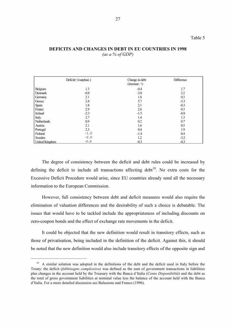
surplus (bt<0 ). Table 5 compares deficits and changes in debt in the EU countries in 1998

(ESA79 figures); as can be seen, the differences are by no means negligible.

17 See Eurostat (1979) and (1995).

27

Table 5

DEFICITS AND CHANGES IN DEBT IN EU COUNTRIES IN 1998(as a % of GDP)

Deficit(+)/surplus(-) Change in debt Difference(increase: +)

Belgium 1.3 -0.4 1.7Denmark -0.8 -3.0 2.2Germany 2.1 1.8 0.3Greece 2.4 5.7 -3.3Spain 1.8 2.1 -0.3France 2.9 2.6 0.3Ireland -2.3 -1.5 -0.8Italy 2.7 1.4 1.3Netherlands 0.9 0.2 0.7Austria 2.1 1.6 0.5Portugal 2.3 0.4 1.9Finland -1.0 -1.4 0.4Sweden -2.0 1.2 -3.2United Kingdom -0.6 -0.3 -0.3

The degree of consistency between the deficit and debt rules could be increased by

defining the deficit to include all transactions affecting debt18. No extra costs for the

Excessive Deficit Procedure would arise, since EU countries already send all the necessary

information to the European Commission.

However, full consistency between debt and deficit measures would also require the

elimination of valuation differences and the desirability of such a choice is debatable. The

issues that would have to be tackled include the appropriateness of including discounts on

zero-coupon bonds and the effect of exchange rate movements in the deficit.

It could be objected that the new definition would result in transitory effects, such as

those of privatisation, being included in the definition of the deficit. Against this, it should

be noted that the new definition would also include transitory effects of the opposite sign and

18 A similar solution was adopted in the definitions of the debt and the deficit used in Italy before the

Treaty: the deficit (fabbisogno complessivo) was defined as the sum of government transactions in liabilitiesplus changes in the account held by the Treasury with the Banca d’Italia (Conto Disponibilità) and the debt asthe total of gross government liabilities at nominal value less the balance of the account held with the Bancad’Italia. For a more detailed discussion see Balassone and Franco (1996).

28

that the present definition already includes some transitory items. Controlling for this type of

measures seems appropriate in any case and is not a trivial problem as can be seen from the

large number of “Eurostat decisions” in the run-up to EMU concerning the proper statistical

treatment of unusual transactions, often carried out to help bring deficit-to-GDP ratios below

the threshold set in the Treaty.

Most importantly, a change in the definition of deficit would have a bearing on the

conceptual framework for stabilisation policy in the EMU. The overall deficit would include

both financial and non-financial transactions. The quantitative effects on economic activity

of transactions belonging to the two sets are presumably different and not always easy to

rank19. Fiscal policy would gain a degree of freedom as its stance would also come to depend

on changes in the relative weights of the two sets of transactions, which could be used

asymmetrically over the cycle. The issue raises the question whether such an outcome would

be desirable or whether stabilisation policy should be restricted to non-financial transactions.

5.3 “Rainy-day funds”

The discussion on the content of “Maastricht” debt and deficit statistics suggests the

third possibility: the introduction of “rainy-day funds” from which resources can be drawn

during cyclical downturns to avoid debt increases.

The use of resources accumulated in this way to reduce gross debt would be fully

consistent with the EMU fiscal rules. Indeed, it is no different from the use of privatisation

receipts or withdrawals from bank deposits, and would be subject to the same rules: rainy-

day funds would not be included in the deficit and would be another component of the ret

term in equation (9)20.

Problems could arise in the build-up of the funds. EMU tax rates are already high by

international standards. Significant expenditure cuts are already needed in order to complete

19 The difference between financial and non-financial transactions is somewhat hazy. For example, it is not

easy to determine unambiguously whether a transfer of resources to a public enterprise is a capital injection (afinancial transaction) or a production/investment subsidy (a non-financial transaction).

20 Rainy-day funds are used by some American States as a shelter against the effects of the cycle on thedeficit in order to comply with balanced budget clauses. This use is not possible under the present EMU rules(see Balassone and Franco, 2000b).

29

the transition towards a balanced structural budget. Raising the funds by borrowing in the

market would clearly not be a solution as it would translate into an increase in gross debt

(unless specific exceptions were agreed upon by the EMU countries).

One possibility would be to use privatisation receipts to build up the funds rather than

using them to reduce outstanding gross liabilities regardless of cyclical conditions.

Obviously, once they had been accumulated, the funds would still have to be

replenished from a “renewable” source of revenue. Here a problem of incentives arises,

similar to the one concerning the budget surpluses that the proper working of the Stability

and Growth Pact requires in favourable cyclical phases.

References

Artis, M.J. and B. Winkler (1997), “The Stability Pact: safeguarding the credibility of theEuropean Central Bank”, CEPR Discussion Papers, No. 1688.

Balassone, F. and D. Franco (1996), “Il fabbisogno finanziario pubblico”, Banca d’Italia,Temi di discussione, No. 277.

_______________________ (2000a), “Assessing fiscal sustainability: a review of methodswith a view to EMU”, in Banca d’Italia (ed.), Fiscal Sustainability – essays presentedat the Bank of Italy workshop, Perugia, 20-22 January 2000, forthcoming.

_______________________ (2000b), “Il federalismo fiscale e il rispetto del Patto distabilità”, proceedings of the conference I controlli delle gestioni pubbliche, Bancad’Italia - Perugia, 2-3 December 1999, forthcoming.

Buti, M., D. Franco and H. Ongena (1997), “Budgetary policies during recessions -Retrospective application of the Stability and Growth Pact to the post-war period”, inRecherches Economiques de Louvain, Vol. 63, No. 4, pp. 321-66.

___________________________ (1998), “Fiscal discipline and flexibility in EMU: theimplementation of the Stability and Growth Pact”, in Oxford Review of EconomicPolicy, Vol. 14, No. 3, pp. 81-97.

Eichengreen, B. and J. Von Hagen (1996), “Fiscal policy and monetary union: federalism,fiscal restrictions, and the no-bailout rule”, in H. Siebert (ed.), Monetary Policy in anIntegrated World Economy - Symposium 1995, Tubingen - Mohr, pp. 212-31.

Eichengreen, B. and C. Wyplosz (1998), “Stability Pact: more than a minor nuisance?”, inEconomic Policy, April, pp. 67-104.

European Commission (1997), “Economic Policy in EMU”, Economic Papers, pp. 124-25.

Eurostat (1979), European System of Accounts, Luxembourg.

_______ (1995), European System of Accounts, Luxembourg.

Pasinetti, L. (1997), European Union at the end of 1997: who is within the public finance“sustainability” zone?, Lezione Lincea “Luigi Einaudi”.

RECENTLY PUBLISHED “TEMI” (*)

No. 351 — Median Voter Preferences, Central Bank Independence and Conservatism, by F.LIPPI (April 1999).

No. 352 — Errori e omissioni nella bilancia dei pagamenti, esportazioni di capitali e aperturafinanziaria dell’Italia, by M. COMMITTERI (June 1999).

No. 353 — Is There an Equity Premium Puzzle in Italy? A Look at Asset Returns, Consumptionand Financial Structure Data over the Last Century, by F. PANETTA and R. VIOLI(June 1999).

No. 354 — How Deep Are the Deep Parameters?, by F. ALTISSIMO, S. SIVIERO andD. TERLIZZESE (June 1999).

No. 355 — The Economic Policy of Fiscal Consolidations: The European Experience, byA. ZAGHINI (June 1999).

No. 356 — What Is the Optimal Institutional Arrangement for a Monetary Union?, byL. GAMBACORTA (June 1999).

No. 357 — Are Model-Based Inflation Forecasts Used in Monetary Policymaking? A CaseStudy, by S. SIVIERO, D. TERLIZZESE and I. VISCO (September 1999).

No. 358 — The Impact of News on the Exchange Rate of the Lira and Long-Term Interest Rates,by F. FORNARI, C. MONTICELLI, M. PERICOLI and M. TIVEGNA (October 1999).

No. 359 — Does Market Transparency Matter? a Case Study, by A. SCALIA and V. VACCA(October 1999).

No. 360 — Costo e disponibilità del credito per le imprese neidistretti industriali, by P. FINALDIRUSSO and P. ROSSI (December 1999).

No. 361 — Why Do Banks Merge?, by D. FOCARELLI, F. PANETTA and C. SALLEO (December1999).

No. 362 — Markup and the Business Cycle: Evidence from Italian Manufacturing Branches,by D. J. MARCHETTI (December 1999).

No. 363 — The Transmission of Monetary Policy Shocks in Italy, 1967-1997, by E. GAIOTTI(December 1999).

No. 364 — Rigidità nel mercato del lavoro, disoccupazione e crescita, by F. SCHIVARDI(December 1999).

No. 365 — Labor Markets and Monetary Union: A Strategic Analysis, by A. CUKIERMAN andF. LIPPI (February 2000).

No. 366 — On the Mechanics of Migration Decisions: Skill Complementarities andEndogenous Price Differentials, by M. GIANNETTI (February 2000).

No. 367 — An Investment-Function-Based Measure of Capacity Utilisation. Potential Outputand Utilised Capacity in the Bank of Italy’s Quarterly Model, by G. PARIGI andS. SIVIERO (February 2000).

No. 368 — Information Spillovers and Factor Adjustment, by L. GUISO and F. SCHIVARDI(February 2000).

No. 369 — Banking System, International Investors and Central Bank Policy in EmergingMarkets, by M. GIANNETTI (March 2000).

No. 370 — Forecasting Industrial Production in the Euro Area, by G. BODO, R. GOLINELLIand G. PARIGI (March 2000).

No. 371 — The Seasonal Adjustment of the Harmonised Index of Consumer Prices for the EuroArea: a Comparison of Direct and Indirect Methods, by R. CRISTADORO andR. SABBATINI (March 2000).

No. 372 — Investment and Growth in Europe and in the United States in the Nineties, byP. CASELLI, P. PAGANO and F. SCHIVARDI (March 2000).

No. 373 — Tassazione e costo del lavoro nei paesi industriali, by M. R. MARINO andR. RINALDI (June 2000).

No. 374 — StrategicMonetaryPolicywithNon-AtomisticWage-SettersbyF.LIPPI(June2000).

(*) Requests for copies should be sent to:Banca d’Italia - Servizio Studi - Divisione Biblioteca e pubblicazioni - Via Nazionale, 91 - 00184 Rome(fax 0039 06 47922059). They are available on the Internet at www.bancaditalia.it