BUYBACK AND TARGET REBATECONTRACTS WHEN THE

MANUFACTURER OPERATES UNDERCARBON CAP AND TRADE MECHANISM

a thesis

submitted to the department of industrial engineering

and the graduate school of engineering and science

of bilkent university

in partial fulfillment of the requirements

for the degree of

master of science

By

Malek Ebadi

July, 2014

I certify that I have read this thesis and that in my opinion it is fully adequate,

in scope and in quality, as a thesis for the degree of Master of Science.

Prof. Dr. Ulku Gurler (Advisor)

I certify that I have read this thesis and that in my opinion it is fully adequate,

in scope and in quality, as a thesis for the degree of Master of Science.

Asst. Prof. Ayse Selin Kocaman

I certify that I have read this thesis and that in my opinion it is fully adequate,

in scope and in quality, as a thesis for the degree of Master of Science.

Asst. Prof. Deniz Yenigun

Approved for the Graduate School of Engineering and Science:

Prof. Dr. Levent OnuralDirector of the Graduate School

ii

ABSTRACT

BUYBACK AND TARGET REBATE CONTRACTSWHEN THE MANUFACTURER OPERATES UNDER

CARBON CAP AND TRADE MECHANISM

Malek Ebadi

M.S. in Industrial Engineering

Supervisor: Prof. Dr. Ulku Gurler

July, 2014

In this study, the coordination of a manufacturer and a retailer in a supply chain

is considered, in a single period environment where the manufacturer has carbon

emission restriction with trade option. The customer demand over a period is

assumed to be a random variable with an arbitrary distribution. Two types of

contracts, namely the buyback and the target rebate contracts are considered. For

each type, the contract parameters which achieve channel coordination have been

studied. The models show that for both contract types, under specific parameter

settings coordination is achievable. In particular, we show that under a buyback

contract with a carbon trader manufacturer, coordination can be achieved, even

if no returns are allowed, contrary to the findings of Pasternack, who first stud-

ied a buyback contract in a setting where carbon emissions are not taken into

consideration. The results are illustrated by numerical examples.

Keywords: Contracts, Newsvendor, Emission Restriction, Cap and Trade, Buy-

back, Target Rebate.

iii

OZET

KARBON TICARETI MEKANIZMASI ALTINDACALISAN BIR URETICI ILE GERI ALMA VE HEDEF

SATIS INDIRIMI KONTRATLARIN ANALIZI

Malek Ebadi

Endustri Muhendisligi, Yuksek Lisans

Tez Yoneticisi: Prof. Dr. Ulku Gurler

Temmuz, 2014

Bu calısmada ureticinin karbon emisyon kısıtı ve karbon ticareti opsiyonu oldugu

bir ticaret zinciri ureticisi ve perakendeci arasındaki tek donemlik koordinasyon

ele alınmıstır. Bir donem icindeki talebin tesadufi degisken oldugu varsayılmıstır.

Geri alma ve hedef satıs olmak uzere iki kontrat tipi incelenmistir. Her kon-

trat tipi icin koordinasyon saglayan sistem parametreleri arastırılmıstır ve belli

kosullar altında koordinasyonun saglandıgı gosterilmistir. Geri alma kontratı

altında, Pasternack’ın bulgularının tersine, geri almaya izin vermeyen ozel du-

rumlarda koordinasyon oldugu gosterilmistir. Sonuclara iliskin numerik ornekler

sunulmustur.

Anahtar sozcukler : Kontratlar, Emisyon Kısıtı, Kota ve Ticaret, Geri Alım, Hedef

Satıs.

iv

Acknowledgement

I would like to take this opportunity to acknowledge the people who have helped

and supported me during the progression of this thesis.

I would like to extend my sincere gratitude to Professor Ulku Gurler and the

other members of the graduate committee, for trusting my ability and offering

me the opportunity to be a part of the Bilkent University. My first memories of

Industrial Engineering department was during the interview session which I will

always carry and enjoy them for the rest of my life. I wish to thank interviewers

for all those friendly faces during that interview. It was a great pleasure to be a

member of the IE department.

I am greatly indebted to Prof. Ulku Gurler, my supervisor, who has helped

me in many ways during these years. She offered her expertise in scientific work

and her kindness in personal contacts. The advice she gave me during the writing

of this thesis was invaluable. She was always available to help with good advice

and suggestions about the thesis. I very much appreciate all her contributions

to this thesis. I am also grateful to the jury members of the thesis, Asst. Prof.

Deniz Yenigun and Asst. Prof. Ayse Selin Kocaman, for their valuable comments

on my thesis manuscript.

All the current and previous members of the IE department deserve thanks

for making the department such a pleasant place for study and creating such a

friendly atmosphere. Further, I thank Ramez Kian and Aysegul Onat for their

support.

Finally, I thank my family, for all the joy and encouragement they have given

me. Special thanks goes to Maryam, for the love, happiness and everything she

did bring and continues to bring into my life.

v

vi

This research is partially supported by TUBITAK grant 110M307.

Contents

1 Introduction 1

1.1 Supply Chain Coordination . . . . . . . . . . . . . . . . . . . . . 1

2 Related Literature 7

2.1 Supply Chain Coordination and Contracts . . . . . . . . . . . . . 7

2.2 Green Supply Chains and Coordination . . . . . . . . . . . . . . . 11

3 Problem Setting and Preliminaries 17

3.1 Buyback Contract . . . . . . . . . . . . . . . . . . . . . . . . . . . 19

3.2 Target Rebate . . . . . . . . . . . . . . . . . . . . . . . . . . . . . 20

3.3 Integrated channel when manufacturer acts as his own retailer . . 21

4 Coordination Under Return Contract 25

4.1 Independent Retailer with Returns . . . . . . . . . . . . . . . . . 26

4.2 Channel Coordination . . . . . . . . . . . . . . . . . . . . . . . . 26

4.2.1 Coordination when Manufacturer Sells Emission Allowance 27

vii

CONTENTS viii

4.2.2 Coordination when Manufacturer Buys Emission Allowance 30

4.2.3 Coordination when Optimal Order is κ/β . . . . . . . . . 32

4.3 Numerical Analysis . . . . . . . . . . . . . . . . . . . . . . . . . . 37

5 Coordination Under Rebate Contract 49

5.1 Independent Retailer With Rebate . . . . . . . . . . . . . . . . . 50

5.2 Channel Coordination . . . . . . . . . . . . . . . . . . . . . . . . 53

5.2.1 Coordination when Manufacturer Sells Emission Allowance 53

5.2.2 Coordination when Manufacturer Buys Emission Allowance 55

5.2.3 Coordination when Manufacturer Produces κ/β Units . . . 56

5.3 Numerical Analysis . . . . . . . . . . . . . . . . . . . . . . . . . . 58

6 Extensions and Conclusion 61

A Appendix 68

List of Figures

1.1 Supply Chain . . . . . . . . . . . . . . . . . . . . . . . . . . . . . 2

3.1 The Optimal Policy for The Channel . . . . . . . . . . . . . . . . 24

4.1 The Scenario Without Returns . . . . . . . . . . . . . . . . . . . 38

4.2 The Optimal Policy at Buying Region with κ < Q∗R . . . . . . . . 38

4.3 The Optimal Policy at Buying Region with Q∗R < κ . . . . . . . . 40

4.4 The Optimal Policy at Selling Region . . . . . . . . . . . . . . . . 41

4.5 The Optimal Policy at ”Do Nothing” Region . . . . . . . . . . . . 44

4.6 Profit of The Retialer Before and After Coordination . . . . . . . 47

4.7 Profit of The Manufacturer Before and After Coordination . . . . 48

5.1 The Scenario Without Rebate . . . . . . . . . . . . . . . . . . . . 58

5.2 Profit of The Manufacturer and Retailer Before and After Coordi-

nation when Manufacturer Sells Extra Allowance . . . . . . . . . 60

ix

List of Tables

4.1 The optimality of the policy for different settings of return rate . 35

4.2 Input Data for The Return Contract . . . . . . . . . . . . . . . . 37

5.1 Input Data for The Rebate Contract . . . . . . . . . . . . . . . . 58

x

Chapter 1

Introduction

1.1 Supply Chain Coordination

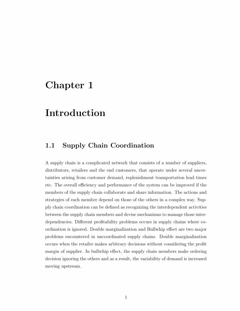
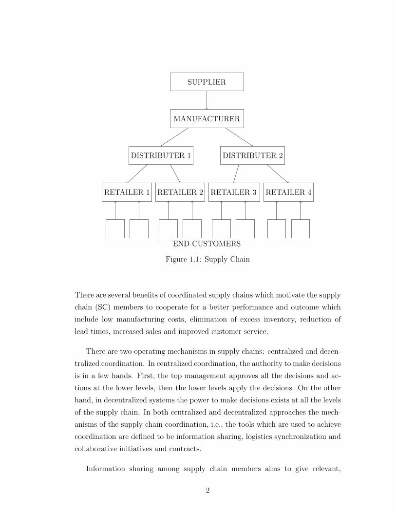
A supply chain is a complicated network that consists of a number of suppliers,

distributors, retailers and the end customers, that operate under several uncer-

tainties arising from customer demand, replenishment transportation lead times

etc. The overall efficiency and performance of the system can be improved if the

members of the supply chain collaborate and share information. The actions and

strategies of each member depend on those of the others in a complex way. Sup-

ply chain coordination can be defined as recognizing the interdependent activities

between the supply chain members and devise mechanisms to manage those inter-

dependencies. Different profitability problems occurs in supply chains where co-

ordination is ignored. Double marginalization and Bullwhip effect are two major

problems encountered in uncoordinated supply chains. Double marginalization

occurs when the retailer makes arbitrary decisions without considering the profit

margin of supplier. In bullwhip effect, the supply chain members make ordering

decision ignoring the others and as a result, the variability of demand is increased

moving upstream.

1

SUPPLIER

MANUFACTURER

DISTRIBUTER 1 DISTRIBUTER 2

RETAILER 2 RETAILER 3RETAILER 1 RETAILER 4

END CUSTOMERS

Figure 1.1: Supply Chain

There are several benefits of coordinated supply chains which motivate the supply

chain (SC) members to cooperate for a better performance and outcome which

include low manufacturing costs, elimination of excess inventory, reduction of

lead times, increased sales and improved customer service.

There are two operating mechanisms in supply chains: centralized and decen-

tralized coordination. In centralized coordination, the authority to make decisions

is in a few hands. First, the top management approves all the decisions and ac-

tions at the lower levels, then the lower levels apply the decisions. On the other

hand, in decentralized systems the power to make decisions exists at all the levels

of the supply chain. In both centralized and decentralized approaches the mech-

anisms of the supply chain coordination, i.e., the tools which are used to achieve

coordination are defined to be information sharing, logistics synchronization and

collaborative initiatives and contracts.

Information sharing among supply chain members aims to give relevant,

2

timely, and accurate information available for decision makers. Information pro-

cessing in organizations includes the gathering of data, the transformation of data

into information, and the communication and storage of information [1].

Logistics synchronization refers to organizing the supply chain according to

the market: to mediate customer demand and to adjust inventory management,

production, and transportation to meet the demand. The synchronizing logistics

processes is also called physical flow coordination. [2].

Among coordination mechanisms, contracts are valuable tools used in both

theory and practice to coordinate various supply chains. According to Tsay [3],

the supply chain contract is a coordination mechanism that provides incentives

to all of its members so that the decentralized supply chain behaves nearly or

exactly the same as the centralized one. By specifying contract parameters such

as quantity, price and lead times, contracts are designed to improve supplier and

buyer relationship. These contracts, based on their type, serve to the different

objectives which include maximizing the total supply chain profit, minimizing the

inventory related costs (overstock and understock) and fair risk sharing between

the members.

Examples of contract types that can be used to achieve coordination, are

returns (buyback), rebate, quantity discounts, quantity flexibility and the use of

subsidies or penalties.

In the next chapter we will discuss each contract type with examples in literature.

In this thesis, we will consider two specific contract types, namely the buyback

contract and target rebate contract in a two echelon supply chain consisting

of a manufacturer and a retailer when the manufacturer has carbon emission

restrictions with trade option. Our research has been motivated by the fact that

1. global warming is becoming a real threat to the world, for which the green-

house gases and especially CO2 are the most significant contributors.

2. There is a global attempt to reduce carbon emissions via several interna-

tional regulations which lead to carbon trading.

3

3. As a result of the above two points new paradigms have been introduced

to the classical problems in the IE/OR context.

To further motivate our problem we provide below some basic information

regarding the international environmental activities to reduce carbon emissions.

Greenhouse gases from human activities are the most significant driver of cli-

mate change since the mid-20th century. As greenhouse gas emissions increase,

they build up in the atmosphere and warm the climate, leading to many other

changes around the world. The Kyoto Protocol to the United Nations Framework

Convention on Climate Change (UNFCCC), agreed in 1997, is an amendment to

the international treaty on climate change, assigning mandatory targets for the

reduction of greenhouse gas. The UNFCCCs Kyoto Protocol authorizes three co-

operative implementation mechanisms: emissions trading, joint implementation

and the clean development mechanism (CDM).

The provision on emissions trading, allows trading of the assigned amounts

of emission. Three distinct trading possibilities emerge from this authorization:

trading among countries with domestic emissions trading systems, trading among

countries without domestic trading systems, and trading among countries with

and without domestic emission trading systems.

The mechanism known as ”joint implementation,” allows a country with an

emission reduction or limitation commitment under the Kyoto Protocol to earn

emission reduction units (ERUs) from an emission-reduction or emission removal

project, each equivalent to one tonne of CO2, which can be counted towards

meeting its Kyoto target.

The clean development mechanism (CDM) allows emission-reduction projects

in developing countries to earn certified emission reduction (CER) credits, each

equivalent to one tonne of CO2. These CERs can be traded and sold, and used

by industrialized countries to a meet a part of their emission reduction targets

under the Kyoto Protocol.

4

EU Emissions Trading System (EU ETS), is the largest multi-country, multi-

sector greenhouse gas emissions trading system in the world. The EU ETS scheme

started in 2005 in order to help the EU meet its targets under the Kyoto Protocol

(8% reduction in greenhouse gas emissions from 1990 levels). The EU ETS works

on the ’cap and trade’ principle. It puts a cap on the carbon dioxide (CO2)

emitted by business and creates a market and price for carbon allowances. It

covers 45% of EU emissions, including energy intensive sectors and approximately

12, 000 installations. The ’Cap’ was converted into allowances, known as EUAs

(1 tonne of Carbon Dioxide = 1 EUA). The carbon price signifies the amount

participants in the EU ETS are willing to pay per EU allowance (1 allowance

(EUA) equals 1 tonne of CO2 or its equivalent) given demand and supply. In

addition, EU Aviation allowances (EUAAs) have been created to be used for

compliance by airline operators.

The trading price differs with programs and the countries which apply the

emission reduction program. Gangadharan [4] studies the Regional Clean Air

Incentives Market (RECLAIM), which is a program implemented in the Los An-

geles to use emissions trading to reduce pollutants in the Los Angeles basin. The

trading price in this program is ranging between $160 and $2220 per ton. In

2008, the European Commission released legislative proposals to cut emissions of

greenhouse gases by 20% and increase the share of renewable energy to 20% of

final energy consumption.

With progression of new developments in the strategies and regulations of

emission reduction, the industries and production companies will also capture

the effects of greening policies in their production and distribution policies and

will be forced into a more competing environment under emission restrictions.

Consumer awareness together with legislation dictated by the government has

also pushed the environmental considerations of a supply chain into spotlight

of the firms, making it mandatory for the organizations to have greening plans.

With regard to the rising global awareness of environmental protection, operations

management researchers started to deal with this problem within a new stream

of research, which is called green supply chain management.

5

Green supply chain management can be defined as the integration of environ-

mental consideration into supply chain management, including material sourcing,

supplier selection, product design, manufacturing processes, packaging, transship-

ment and delivery to the end consumers [5]. The OR researchers have considered

green supply chain management from different perspectives. In the next chapter,

we will present examples of literature work related to the inventory management

problems considering greening policies.

In compliance with the emission reduction considerations, we have build our

model based on a supply chain with carbon restricted manufacturer. The model is

constructed under two contract types, namely buyback(return) and target rebate

contracts. For the return contract, in which a proportion of unsold items is

allowed to be returned, we found that even if the manufacturer allows no returns,

under special conditions the channel may be coordinated. For the case of no

returns, we derived the optimal wholesale price and the conditions for return

rate and price which are required for coordination in each of the order range.

We showed that when full return is allowed, if the return price is lower than the

wholesale price, there are pricing schemes which leads to overall channel benefit

and coordination in particular.

For the rebate contract, in which the retailer gets a certain credit for the sales

beyond a target, we have derived the optimal state of each contract parameter.

We have performed this analysis for each case corresponding to the assigned

emission cap. The results show that a properly designed target rebate achieves

coordination and a win-win outcome.

This thesis is organized as follows: In chapter 2, we presents an overview of

the literature related to this research. In Chapter 3, the two models are discussed

and the preliminaries are presented. In Chapter 4, we deal with the model, in

which we focus on the coordination of a manufacturer and a retailer under return

contract. In Chapter 5, the model with rebate contract is developed. Finally, in

chapter 6, we summarize the findings, draw conclusions, and point out avenues

for future research.

6

Chapter 2

Related Literature

2.1 Supply Chain Coordination and Contracts

In this chapter we classified the current literature relevant to the core concepts

in this work and, based on the gap in the literature, our motivation behind this

study is explained.

An example of a coordinating contract for the newsvendor setting is the buy-

back or markdown contract. In this contract, the manufacturer reduces the risk

of overage for the retailer by offering to buy back a part of the stock that is not

sold at a certain price . In this way, the buyer’s full order quantity is partially

protected against not selling. The cost per item due to overage decreases and the

retailer orders more.

Pasternack [6], in a newsvendor structure described in paragraph one of chapter

three , for a commodity with short shelf or demand life develops a hierarchical

model for deciding the optimal pricing policy for the manufacturer. In his model,

manufacturer has the control of channel and is free to set the pricing policy.

Goodwill cost is incurred by both the retailer and the manufacturer. He shows

that the pricing policy with full credit for all unsold items as well as the pol-

icy with no returns could not achieve coordination. He concludes that under a

properly chosen wholesale price, full credit for partial returns in a single retailer

7

and partial credit for unlimited returns in a multi retailer environment is channel

coordinated. However, in the case of multi retailer environment all retailers are

not affected equally.

Lariviere and Porteus [7] discuss a return policy in a single manufacturer

and retailer channel using the newsvendor-type demand. Results show that the

unrestricted return quantity policy is independent of the demand distribution.

They do not consider supply chain coordination in their model.

Wu [8] studies the impact of buyback policy on retail price, order quantity

and wholesale price in a duopoly of two manufacturer-retailer supply chains using

newsvendor model. He assumes a competing supply chain in which the manu-

facturer maximizes its profit under its own optimal choice of a wholesale price.

Given the wholesale price, the retailer makes the procurement determination and

obtain the purchasing items from the manufacturer and resells them at the retail

level with a self-determined price. He examines both buyback and non-buyback

policies for two competing supply chains using vertical integration (VI) and man-

ufacturer Stackelberg (MS) game methods. The results show that in the VI case

with buyback policy, the manufacturer and retailer act as the same agent to set

up a return policy and decide on ordering quantity and retail price.

Xiao et.al. [9] Consider coordination of a supply chain consisting of one manu-

facturer and one retailer facing consumer return. They integrate consumer returns

policy and manufacturer buyback policy within a modeling framework. They de-

sign a buyback/markdown money contract to coordinate the supply chain under

partial refund policy. They show that the refund amount plays an important role

in the decisions and profitability of the players. In the coordinated setting with

given buyback price, the refund amount first increases the players’ expected prof-

its/quantity, and then decreases them. When the risk of the consumer’s return

increases, the manufacturer may increase the unit wholesale price to achieve a

higher unit profit. They show that the supply chain is better off using full refund

policy if the risk is very small; otherwise, the supply chain prefers no returns

policy.

In the case of a sales-rebate contract, the manufacturer provides an incentive

8

for each item that is sold above a certain threshold.

Taylor [10] considers a contract with time restricted rebates in which manufac-

turer specifies wholesale price and a rebate value and then, the retailer chooses

the order quantity. In his model wholesale price is linear in order quantity. Selling

price, manufacturing cost and salvage value are exogenous and wholesale price,

rebate value and sale threshold are endogenous. In the attempt to explore the

role of rebates in a one period model, two different structure is analyzed. The

model in which retailer deals only with order quantity issue and the model with

order quantity plus sales effort effect. His findings show that when demand is not

influenced by sales effort, properly designed target rebate achieves channel coor-

dination. However if sales effort affects retailers demand, then properly designed

target rebate plus returns contract achieves channel coordination.

Wong et al. [11] develop a model in the context of a two-echelon supply

chain with a single supplier serving multiple retailers in vendor-managed inven-

tory (VMI) partnership. In their model retailers are considered in two scenarios:

independent retailers with a demand function sensitive only to their own price

and competing retailers with a demand function depending on all retailers’ prices.

Their proposed model demonstrates that the supplier gains more profit with com-

peting retailers than without as competition among the retailers lowers the prices

and thus stimulates demand.

Another, closely related agreement is the revenue sharing contract. In this

case, the retailer pays the manufacturer a wholesale price per unit plus a per-

centage of the revenue the retailer generates. In the video cassette rental industry,

such contracts are commonly used.

Cachon and Lariviere [12] showed that under a revenue-sharing contract, the man-

ufacturer will set a wholesale price below production cost if manufacturer and re-

tailer agree to share the total revenue of the supply chain. They also showed that

buyback contracts and revenue-sharing contracts are equivalent in the fixed-price

newsvendor model; for any buyback contract, there exists a revenue-sharing con-

tract that generates the same cash flows for any realization of demand. However,

this is not the case when demand is price-dependent. They study the impact

9

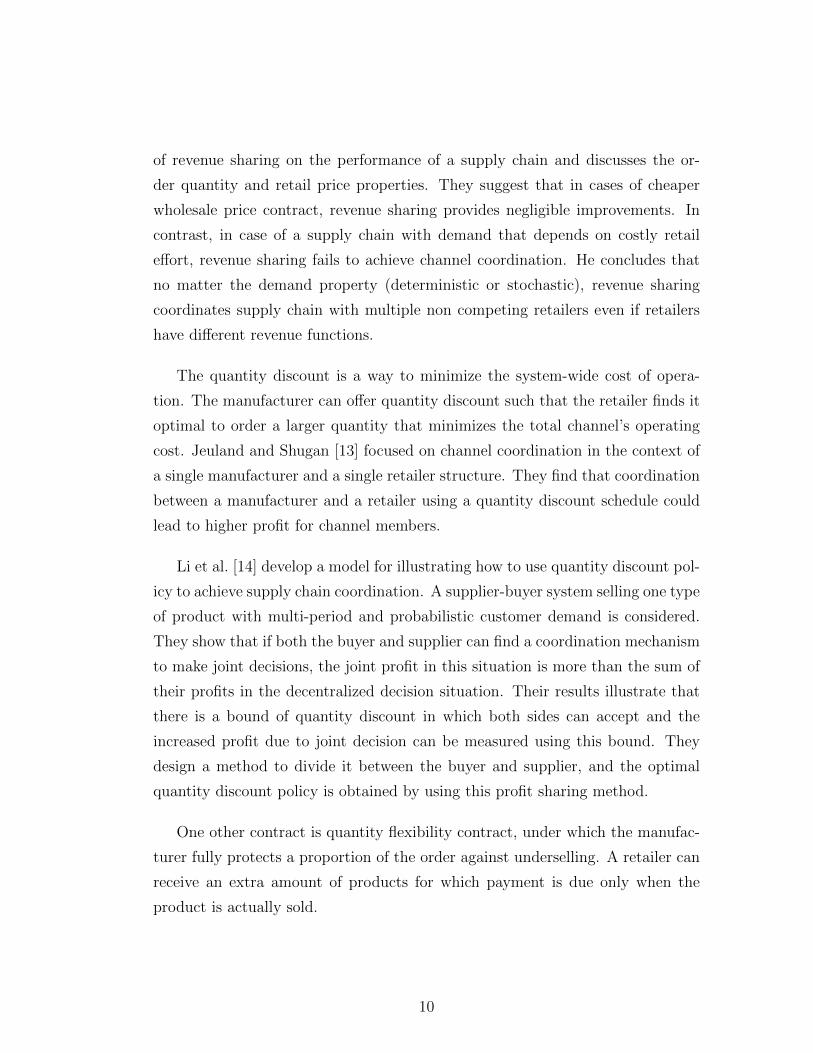
of revenue sharing on the performance of a supply chain and discusses the or-

der quantity and retail price properties. They suggest that in cases of cheaper

wholesale price contract, revenue sharing provides negligible improvements. In

contrast, in case of a supply chain with demand that depends on costly retail

effort, revenue sharing fails to achieve channel coordination. He concludes that

no matter the demand property (deterministic or stochastic), revenue sharing

coordinates supply chain with multiple non competing retailers even if retailers

have different revenue functions.

The quantity discount is a way to minimize the system-wide cost of opera-

tion. The manufacturer can offer quantity discount such that the retailer finds it

optimal to order a larger quantity that minimizes the total channel’s operating

cost. Jeuland and Shugan [13] focused on channel coordination in the context of

a single manufacturer and a single retailer structure. They find that coordination

between a manufacturer and a retailer using a quantity discount schedule could

lead to higher profit for channel members.

Li et al. [14] develop a model for illustrating how to use quantity discount pol-

icy to achieve supply chain coordination. A supplier-buyer system selling one type

of product with multi-period and probabilistic customer demand is considered.

They show that if both the buyer and supplier can find a coordination mechanism

to make joint decisions, the joint profit in this situation is more than the sum of

their profits in the decentralized decision situation. Their results illustrate that

there is a bound of quantity discount in which both sides can accept and the

increased profit due to joint decision can be measured using this bound. They

design a method to divide it between the buyer and supplier, and the optimal

quantity discount policy is obtained by using this profit sharing method.

One other contract is quantity flexibility contract, under which the manufac-

turer fully protects a proportion of the order against underselling. A retailer can

receive an extra amount of products for which payment is due only when the

product is actually sold.

10

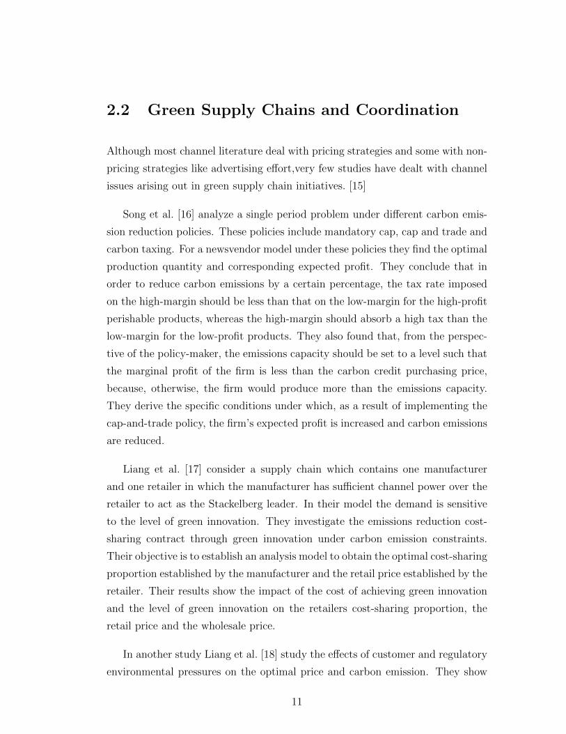
2.2 Green Supply Chains and Coordination

Although most channel literature deal with pricing strategies and some with non-

pricing strategies like advertising effort,very few studies have dealt with channel

issues arising out in green supply chain initiatives. [15]

Song et al. [16] analyze a single period problem under different carbon emis-

sion reduction policies. These policies include mandatory cap, cap and trade and

carbon taxing. For a newsvendor model under these policies they find the optimal

production quantity and corresponding expected profit. They conclude that in

order to reduce carbon emissions by a certain percentage, the tax rate imposed

on the high-margin should be less than that on the low-margin for the high-profit

perishable products, whereas the high-margin should absorb a high tax than the

low-margin for the low-profit products. They also found that, from the perspec-

tive of the policy-maker, the emissions capacity should be set to a level such that

the marginal profit of the firm is less than the carbon credit purchasing price,

because, otherwise, the firm would produce more than the emissions capacity.

They derive the specific conditions under which, as a result of implementing the

cap-and-trade policy, the firm’s expected profit is increased and carbon emissions

are reduced.

Liang et al. [17] consider a supply chain which contains one manufacturer

and one retailer in which the manufacturer has sufficient channel power over the

retailer to act as the Stackelberg leader. In their model the demand is sensitive

to the level of green innovation. They investigate the emissions reduction cost-

sharing contract through green innovation under carbon emission constraints.

Their objective is to establish an analysis model to obtain the optimal cost-sharing

proportion established by the manufacturer and the retail price established by the

retailer. Their results show the impact of the cost of achieving green innovation

and the level of green innovation on the retailers cost-sharing proportion, the

retail price and the wholesale price.

In another study Liang et al. [18] study the effects of customer and regulatory

environmental pressures on the optimal price and carbon emission. They show

11

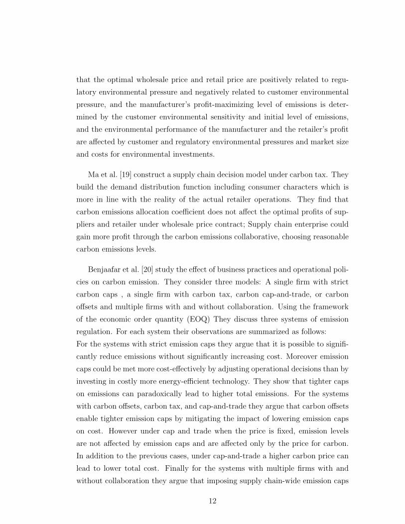
that the optimal wholesale price and retail price are positively related to regu-

latory environmental pressure and negatively related to customer environmental

pressure, and the manufacturer’s profit-maximizing level of emissions is deter-

mined by the customer environmental sensitivity and initial level of emissions,

and the environmental performance of the manufacturer and the retailer’s profit

are affected by customer and regulatory environmental pressures and market size

and costs for environmental investments.

Ma et al. [19] construct a supply chain decision model under carbon tax. They

build the demand distribution function including consumer characters which is

more in line with the reality of the actual retailer operations. They find that

carbon emissions allocation coefficient does not affect the optimal profits of sup-

pliers and retailer under wholesale price contract; Supply chain enterprise could

gain more profit through the carbon emissions collaborative, choosing reasonable

carbon emissions levels.

Benjaafar et al. [20] study the effect of business practices and operational poli-

cies on carbon emission. They consider three models: A single firm with strict

carbon caps , a single firm with carbon tax, carbon cap-and-trade, or carbon

offsets and multiple firms with and without collaboration. Using the framework

of the economic order quantity (EOQ) They discuss three systems of emission

regulation. For each system their observations are summarized as follows:

For the systems with strict emission caps they argue that it is possible to signifi-

cantly reduce emissions without significantly increasing cost. Moreover emission

caps could be met more cost-effectively by adjusting operational decisions than by

investing in costly more energy-efficient technology. They show that tighter caps

on emissions can paradoxically lead to higher total emissions. For the systems

with carbon offsets, carbon tax, and cap-and-trade they argue that carbon offsets

enable tighter emission caps by mitigating the impact of lowering emission caps

on cost. However under cap and trade when the price is fixed, emission levels

are not affected by emission caps and are affected only by the price for carbon.

In addition to the previous cases, under cap-and-trade a higher carbon price can

lead to lower total cost. Finally for the systems with multiple firms with and

without collaboration they argue that imposing supply chain-wide emission caps

12

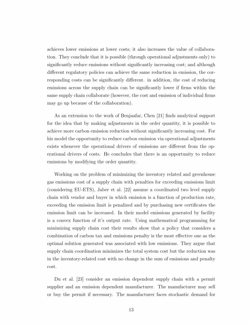
achieves lower emissions at lower costs; it also increases the value of collabora-

tion. They conclude that it is possible (through operational adjustments only) to

significantly reduce emissions without significantly increasing cost; and although

different regulatory policies can achieve the same reduction in emission, the cor-

responding costs can be significantly different. in addition, the cost of reducing

emissions across the supply chain can be significantly lower if firms within the

same supply chain collaborate (however, the cost and emission of individual firms

may go up because of the collaboration).

As an extension to the work of Benjaafar, Chen [21] finds analytical support

for the idea that by making adjustments in the order quantity, it is possible to

achieve more carbon emission reduction without significantly increasing cost. For

his model the opportunity to reduce carbon emission via operational adjustments

exists whenever the operational drivers of emissions are different from the op-

erational drivers of costs. He concludes that there is an opportunity to reduce

emissions by modifying the order quantity.

Working on the problem of minimizing the inventory related and greenhouse

gas emissions cost of a supply chain with penalties for exceeding emissions limit

(considering EU-ETS), Jaber et al. [22] assume a coordinated two level supply

chain with vendor and buyer in which emission is a function of production rate,

exceeding the emission limit is penalized and by purchasing new certificates the

emission limit can be increased. In their model emissions generated by facility

is a convex function of it’s output rate. Using mathematical programming for

minimizing supply chain cost their results show that a policy that considers a

combination of carbon tax and emissions penalty is the most effective one as the

optimal solution generated was associated with low emissions. They argue that

supply chain coordination minimizes the total system cost but the reduction was

in the inventory-related cost with no change in the sum of emissions and penalty

cost.

Du et al. [23] consider an emission dependent supply chain with a permit

supplier and an emission dependent manufacturer. The manufacturer may sell

or buy the permit if necessary. The manufacturer faces stochastic demand for

13

a single product. No return, salvage and inventory holding costs are assumed.

They game theoretically analyze the optimal decisions in a cap and trade system.

They argue that in the modeling of Stackelberg game there is a Nash equilibrium

where both parties achieve the maximum profit. The manufacturer’s profit as well

as the system-wide profit increase as the cap increase but the permit supplier’s

profit decrease. In their model under special conditions there will be room for the

emission dependent manufacturer and permit supplier to coordinate to get more

profit per production. They also employed Bernoulli-Nash social welfare function

to analyze the optimal cap. Based on their findings the system wide and the

manufacturer’s profit increase with the emission cap while the permit supplier’s

decrease.

Ghosh and Shah [15] examine an apparel serial supply chain whose players

initiate product greening. They consider situations in which the players cooper-

ate or act individually. Their study is based on the clothing industry with short

shelf/demand life. Using game theoretic models they build a two-part tariff con-

tract to coordinate the green channel made of one manufacturer and one retailer.

The demand is a linear function of retail price and the level of green innova-

tion. They argue that cooperation between players does lead to higher greening

levels as seen in market structures, manufacturer Stackelberg cooperative policy

(MSCP) and vertical Nash cooperative policy (VNCP), however greening leads

to higher retail prices of the apparel. The findings necessitate support from gov-

ernments and policy making bodies which need to provide suitable incentives to

companies going green in order to lower the prices of green apparels. Further,

contrary to expectations, although cooperation through bargaining is advanta-

geous to the overall supply chain and the retailer in certain market structures,

the manufacturer does not benefit through cooperation and there is a need for the

retailer to provide suitable incentives to the manufacturer for him to participate

in the bargaining process.

Hua et al. [24] studied how firms manage carbon footprints in inventory man-

agement under the cap-and-trade mechanism. Their research focuses on the car-

bon emissions caused by logistics and warehousing activities. They assume that

the carbon emissions from logistics per order is linear in the order quantity and the

14

carbon emissions from warehouse is linear in the inventory and the carbon price

is not affected by the carbon cap allocated to a single retailer. They compared

the optimal decision under cap and trade with that for the classical EOQ model,

and examined the impacts of carbon cap and carbon price on order size, carbon

emissions, and total cost. They argue that the optimal order size is between the

optimal EOQ order size and the order size that minimizes carbon emissions. They

show that compared with the classical EOQ model, the cap-and-trade mechanism

induces the retailer to reduce carbon emissions, which may result in an increase

in the total cost. However, the retailer may reduce carbon footprints and total

cost simultaneously under some conditions. Carbon cap and carbon price have a

great impact on the retailers order decisions, carbon footprints, and total cost. In

their model whether the retailer should buy carbon credit depends on the carbon

cap as follows: when the cap is less (higher) than a threshold, the retailer should

buy (sell) carbon credit, whereas when the cap equals the threshold, he should

neither buy nor sell. With increasing carbon price, the retailer may order more

or fewer products, which depends on the cost and carbon emissions from logistics

and warehouse. With increasing carbon price, the total cost may increase or de-

crease, depending on the carbon cap. When the cap is lower than one threshold,

the total cost will increase; when the cap is higher than another higher threshold,

the total cost will decrease; and when the cap is between the two thresholds, the

cost will initially increase and then decrease.

Zhang et al. [25] study a supply chain with a permission dependent manufac-

turer and a retailer. The manufacturer has an emission quota predetermined by

the government. Beside the permission for carbon trading under cap and trade

regulation, they consider single and multi time purification in their model. Within

such a structure they aim to maximize the expected profit with appropriate pro-

duction scale. In other words, for each purification case they find the optimal

production quantity to balance the trade-off between purchase and purification.

Zanoni et al. [26] developed a joint economic lot sizing model for coordinated

inventory replenishment decisions for price and environmentally sensitive demand.

In their model two parameters are associated with the environmental performance

and sensitivity of the demand to the environmental considerations. Using (Q,R)

15

model they deal with the vendor’s production lot size, selling price and the capital

invested to improve product quality.

Toptal et al. [27] study a retailer’s joint decisions on inventory replenishment

and carbon emission reduction investment under three carbon emission regulation

policies. They extend the economic order quantity model to consider carbon

emissions reduction investment availability under carbon cap, tax and cap-and-

trade policies. They analytically show that carbon emission reduction investment

opportunities, additional to reducing emissions as per regulations, further reduce

carbon emissions while reducing costs. They provide an analytical comparison

between various investment opportunities and compare different carbon emission

regulation policies in terms of costs and emissions.

Swami et al. [28] discusses the problem of coordination of a manufacturer

and a retailer in a vertical supply chain, who consider greening actions in their

operations. They address some pertinent questions in this regard such as extent

of effort in greening of operations by manufacturer or retailer, level of cooperation

between the two parties, and how to coordinate their operations in a supply chain.

The greening efforts by the manufacturer and retailer result in demand expansion

at the retail end. The decision variables of the manufacturer are wholesale price

and greening effort, while those of the retailer are retail price and its greening

effort. They show that the ratio of the optimal greening efforts put in by the

manufacturer and retailer is equal to the ratio of their green sensitivity ratios

and greening cost ratios. Further, profits and efforts are higher in the integrated

channel as compared to the case of the decentralized channel. Finally, they define

a two-part tariff contract to produce channel coordination.

From the above review we observe that there is a gap in the literature re-

garding different contracts under carbon restrictions and trading. We therefore

attempt to fill in this gap by considering two alternative contracts. In particular,

we obtain the parameter settings under which the supply chain coordinates both

with buy-back and target rebate contracts.

16

Chapter 3

Problem Setting and

Preliminaries

One of the classical problems in the inventory management literature is the

newsvendor problem. Consider a retailer who places an order for a single product

at the beginning of each period. The quantity procured is used solely to satisfy

demand during the current period. No inventory is kept from one period to the

next. The demand for this product during the current period is not known in

advance. Instead, it is represented by a non-negative random variable X. The

probability density function is f(X) and the cumulative distribution function of

X is F, i.e., F (X) = P (X ≤ x). The retailer must determine the order quantity

Q which minimizes the expected cost at the end of the period. There are two

cost components associated with the newsvendor problem, overstock cost Co and

understock cost Cu. The objective of the newsvendor problem is to find the op-

timal order quantity which minimizes the expected total cost. The newsvendor

problem is suitable for the inventory management systems of perishable goods

which can not be carried from one period to another. Newspaper, grocery items

like milk, food and any other item with short shelf or demand life that can be pur-

chased only once in a selling season are examples of perishable goods. Whitin [29]

first presented the newsvendor problem. Since then, there has been a growing

17

interest in the model with it’s various versions in the literature of inventory man-

agement. Many extension has been proposed to the newsvendor problem. Lau

and Lau [30], Khouja [31] and Shore [32] have considered the newsvendor prob-

lem from different perspectives and extended the results to different settings of

supply chain.

In this research we have considered two problems, referring to two contracts

under the newsvendor setting. The decentralized objective functions of the man-

ufacturer and retailer are expected profits. The aim of the study is to find the

contract parameters to harmonize their manufacturing and ordering quantities

and maximizing their expected profit. Such parameters are said to coordinate

the channel. For each contract the optimal ordering quantities of the manufac-

turer and the retailer is found, then the contract parameters are set such that

these quantities are equal. After coordinating the orders, we look for the special

set of parameters which result in a win-win outcome in terms of expected profit

for both retailer and manufacturer.

In our model, under the newsvendor setting, the manufacturer produces an

item with short life cycle for sale to the retailer. Each unit of production emits

β units of carbon dioxide. The manufacturer has an emission allowance (cap)

κ in each production period. However the carbon trading regulation enables

the manufacturer to compensate deficiency and sufficiency of carbon through

the carbon market. The κ value can be considered as a cap imposed by the

government or the environmental organizations. Selling and buying prices of the

carbon in the carbon market are assumed to be ps and pb respectively. The

conventional relation between selling and buying prices is such that, the buying

price is costly than the selling price to the carbon market. Let Q represent the

production quantity of the manufacturer. We assumed that unit item production

emits β units of carbon dioxide. As a result Qβ units of carbon will be emitted

if Q items are produced. If the specified κ by the government is greater than

Qβ , then selling of the remaining (κ − Qβ) with ps to the carbon market will

add (κ − Qβ)ps to the channel profit. In return, a κ value less than Qβ pushes

the manufacturer to compensate the shortcoming of (Qβ − κ) from the carbon

market with a price of pb. This will reduce the channel profit by (Qβ − κ)pb.

18

The manufacturer has to decide on the wholesale price to the retailer. The

wholesale price to charge for the product depends on the cost function and market

bear in terms of price. Once the price is set, retailer decides on the amount of

order quantity. Retailer places the orders once in a selling period and sells during

the selling period. The lead time is assumed to be negligible.

Under two contract types between manufacturer and retailer, namely return

and rebate we set the contract parameters in such a way that the manufacturer

and retailer have the same production and order quantity.

3.1 Buyback Contract

For the contract with returns of the unsold items, the scenario is as follows:

The retailer places an order of size Q at the beginning of a selling season. The

manufacturer sells the finished item to the retailer with wholesale price c1 and

allows the retailer to return some or all of the unsold items at the end of selling sea-

son. Before the procurement of the order quantity, the manufacturer announces

the price c2 which he pays to the retailer for the unsold items. Considering his

expected profit margin, the retailer decides on the end-customer selling price p.

Beside the order amount one other important decision to make is whether to let

the retailer to return some or all of the remained items at the end of a selling

season. That is, the retailer in return of a certain credit returns a proportion

0 ≤ R ≤ 1 of inventory on hand to the manufacturer for the disposal with sal-

vage value c3 and the target is achieving coordination by letting such a return

policy.

The following relations are assumed to hold: A1) c3 < c < c1 < p and A2)

c3 < c2 ≤ c1 < p.

The goodwill cost associated with the end customer’s unsatisfied demand is

partially incurred by retailer g and partially by the manufacturer g1. The total

goodwill cost is g2 = g + g1. The order quantity affects the total profit of the

19

manufacturer. The contract parameters which need to be optimized in order to

set coordination are:

i) The price charged to the retailer per unit product, i.e., c1.

ii) The per unit credit for returned items paid by manufacturer to retailer, i.e.,

c2.

iii) The percentage of unsold allowed to be returned, i.e., R.

Pasternack [6] was the first researcher who considered coordination with buy-

back contract. In his model, when the manufacturer permits no return, the

channel turns out to be uncoordinated. This is true for the case of full returns

with full credit as well. However, for a single retailer when full return is allowed

and the return price is smaller than the wholesale price, then under a specific

relation between wholesale and return price, coordination is achievable.

3.2 Target Rebate

In addition to return contracts, channel rebates are also common mechanisms

for manufacturers to entice retailers to increase their order quantities and sales

ultimately. Rebate is different from discount. Rebate is the money paid by

manufacturer to the retailer for the units sold. This could be linear rebate or

target rebate. In linear rebate manufacturer pays retailer a rebate for each unit

sold. Target rebate is the money paid by manufacturer to the retailer for the

sales beyond a target T . Linear rebate is a converse contract type of revenue

sharing contract in the sense that in revenue sharing retailer pays manufacturer

a portion of retail price for each unit sold to the customer.

Manufacturer sells the items to the retailer with wholesale price c1. Based

on the target rebate contract, the manufacturer pays the rebate amount u to the

retailer for the sales beyond a specific target T . These three values are the system

or contract parameters which we studied to find the optimal values which lead to

coordination.

Selling, manufacturing and salvage prices are assumed to be exogenous and

20

wholesale price;c1, rebate value; u and target sale; T are assumed to be endoge-

nous. No lump sum side payment is allowed. The order quantity is chosen by the

retailer after the manufacturer specifies the rebate amount. The followings are

assumed: B1) 0 < c < c1 < p and B2) c3 < c, u > 0, T > 0

Furthermore we assume that the goodwill cost corresponding to the lost demand

is negligible, g = g1 = 0 as in Taylor.

According to the structure of the rebate contract no returns is allowed. That

is, for the rebate contract R = 0 and c2 = 0. The contract parameters which

need to be optimized in order to set coordination are:

i) The price charged to the retailer per unit product, i.e., c1.

ii) The target sales, i.e., T .

iii) The rebate for the sales beyond target, i.e., u.

All the notations used in the thesis is given in Appendix.

3.3 Integrated channel when manufacturer acts

as his own retailer

When the manufacturer directly sells to the market without any retailer, then

the expected channel’s profit is given by:

EPT (Q) = −cQ+

∫ Q

0

[xp+ (Q− x)c3]f(x)dx+

∫ ∞Q

[pQ− g2(x−Q)]f(x)dx

+[m(κ−Qβ)ps] + [(1−m)(κ−Qβ)pb] (3.1)

where m = 1 if κ > Qβ, zero otherwise.

The newsvendor model with resource constraints have been studied earlier

by Sozuer [33] and Korkmaz [34] in their thesis. However we provide below the

21

optimization results for the sake of completeness.

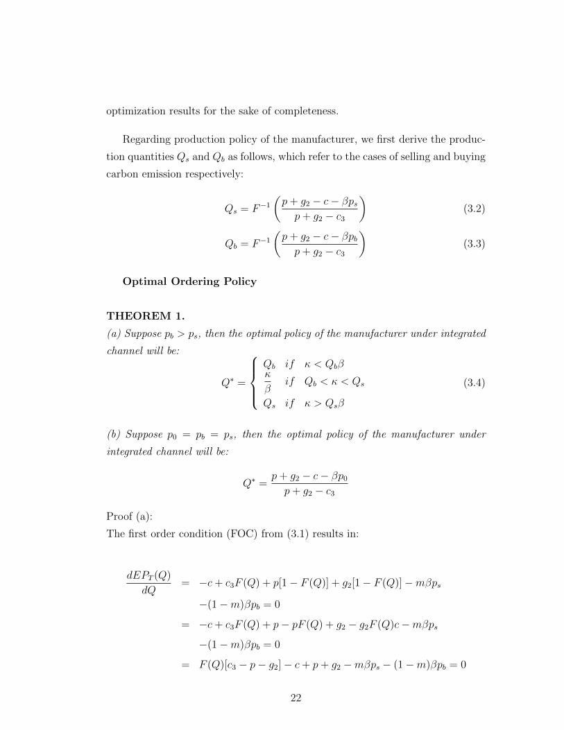
Regarding production policy of the manufacturer, we first derive the produc-

tion quantities Qs and Qb as follows, which refer to the cases of selling and buying

carbon emission respectively:

Qs = F−1(p+ g2 − c− βpsp+ g2 − c3

)(3.2)

Qb = F−1(p+ g2 − c− βpbp+ g2 − c3

)(3.3)

Optimal Ordering Policy

THEOREM 1.

(a) Suppose pb > ps, then the optimal policy of the manufacturer under integrated

channel will be:

Q∗ =

Qb if κ < Qbβκ

βif Qb < κ < Qs

Qs if κ > Qsβ

(3.4)

(b) Suppose p0 = pb = ps, then the optimal policy of the manufacturer under

integrated channel will be:

Q∗ =p+ g2 − c− βp0p+ g2 − c3

Proof (a):

The first order condition (FOC) from (3.1) results in:

dEPT (Q)

dQ= −c+ c3F (Q) + p[1− F (Q)] + g2[1− F (Q)]−mβps

−(1−m)βpb = 0

= −c+ c3F (Q) + p− pF (Q) + g2 − g2F (Q)c−mβps−(1−m)βpb = 0

= F (Q)[c3 − p− g2]− c+ p+ g2 −mβps − (1−m)βpb = 0

22

which implies:

F (Q) =c− p− g2 +mβps + (1−m)βpb

c3 − p− g2Qs is the optimal production quantity if the excess carbon is sold in the carbon

market and Qb is the optimal production quantity if additional carbon emission

allowance is purchased from the carbon market. Then

F (Qs) =c− p− g2 + βpsc3 − p− g2

=p+ g2 − c− βpsp+ g2 − c3

F (Qb) =c− p− g2 + βpbc3 − p− g2

=p+ g2 − c− βpbp+ g2 − c3

and we get

Qs = F−1(p+ g2 − c− βpsp+ g2 − c3

)Qb = F−1

(p+ g2 − c− βpbp+ g2 − c3

)

Assuming pb > ps we have

c− p− g2 + βpsc3 − p− g2

>c− p− g2 + βpbc3 − p− g2

p+ g2 − c− βpsp+ g2 − c3

>p+ g2 − c− βpbp+ g2 − c3

Since F is a one to one and increasing function, we have

F−1(p+ g2 − c− βpsp+ g2 − c3

)> F−1

(p+ g2 − c− βpbp+ g2 − c3

)which implies Qs > Qb.

The first and second order conditions of the expected profit function of the inte-

grated channel for two cases of buying and selling will be:

dEPT (Q)

dQ=

−c+ c3F (Q) + p[1− F (Q)] + g2[1− F (Q)]− βps

−c+ c3F (Q) + p[1− F (Q)] + g2[1− F (Q)]− βpb

23

d2EPT (Q)

dQ2=

c3f(Q)− pf(Q)− g2f(Q) = −f(Q) (p+ g2 − c3) < 0

c3f(Q)− pf(Q)− g2f(Q) = −f(Q) (p+ g2 − c3) < 0

Obviously either κ > Qβ or κ < Qβ , the second derivative is negative. Con-

sequently the Qs and Qb values are the extreme values. Based on this we can

define the optimal policy of the channel for different ranges of κ; The important

issue to be considered is that, what the policy must be when the κ ; is between

Qb/β and Qs/β. Note that in this case the optimal order quantity will be κ/β;

therefore the manufacturer needs nor to sell neither to buy any carbon emission

limit. Based on these results, the policy is as given.

Proof (b): Result follows from part (a) when we let ps = pb.

Remark:

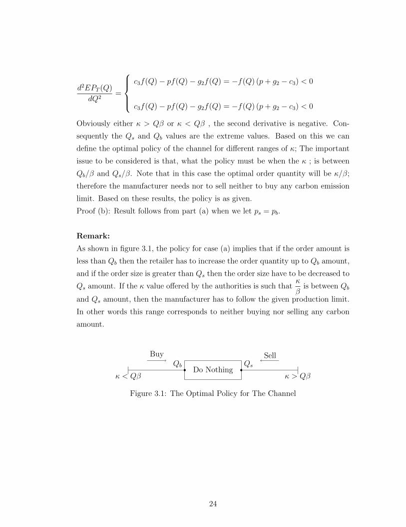
As shown in figure 3.1, the policy for case (a) implies that if the order amount is

less than Qb then the retailer has to increase the order quantity up to Qb amount,

and if the order size is greater than Qs then the order size have to be decreased to

Qs amount. If the κ value offered by the authorities is such thatκ

βis between Qb

and Qs amount, then the manufacturer has to follow the given production limit.

In other words this range corresponds to neither buying nor selling any carbon

amount.

Do Nothing

Buy SellQb Qs

κ > Qβκ < Qβ

Figure 3.1: The Optimal Policy for The Channel

24

Chapter 4

Coordination Under Return

Contract

Introduction

This chapter considers the pricing decision faced by the manufacturer. According

to the return contract, the retailer may return some or all the unsold items at

the end of the selling season. This percentage is denoted by R.

The manufacturer’s policy involves three decision variables, namely the whole-

sale price c1, return price c2 and the return percentage R. Recall that we assume

c2 ≤ c1. In the remaining part of this chapter, the setting which results in coor-

dination in terms of the expected profit between manufacturer and retailer will

be discussed.

25

4.1 Independent Retailer with Returns

Expected profit function of the independent retailer with returns:

EPR(Q) = −c1Q+

∫ (1−R)Q

0

[xp+RQc2 + ((1−R)Q− x) c3]f(x)dx

+

∫ Q

(1−R)Q

[xp+ (Q− x)c2]f(x)dx+

∫ ∞Q

[pQ− (x−Q)g]f(x)dx

(4.1)

Using the first order condition (FOC):dEPR(Q)

dQ= 0

−c1 + p+ g − F (Q)[p+ g − c2]− [(1−R)(c2 − c3)]F ((1−R)Q) = 0

which implies that optimal ordering quantity must satisfy the following

F (Q)[p+ g − c2] + [(1−R)(c2 − c3)]F ((1−R)Q) = p+ g − c1 (4.2)

4.2 Channel Coordination

To achieve channel coordination the retailer’s order amount must be equal to

the optimal production amount of integrated channel. In other words, we search

for the parameter setting that will result in the same optimal quantity of the

integrated channel and the retailer. Since the manufacturer’s optimal policy has

three regions where optimal production quantities are given by Qs, Qb andκ

β, we

will consider coordination in these three regions separately. In the remaining of

this section we used coordination and optimal in the same meaning.

26

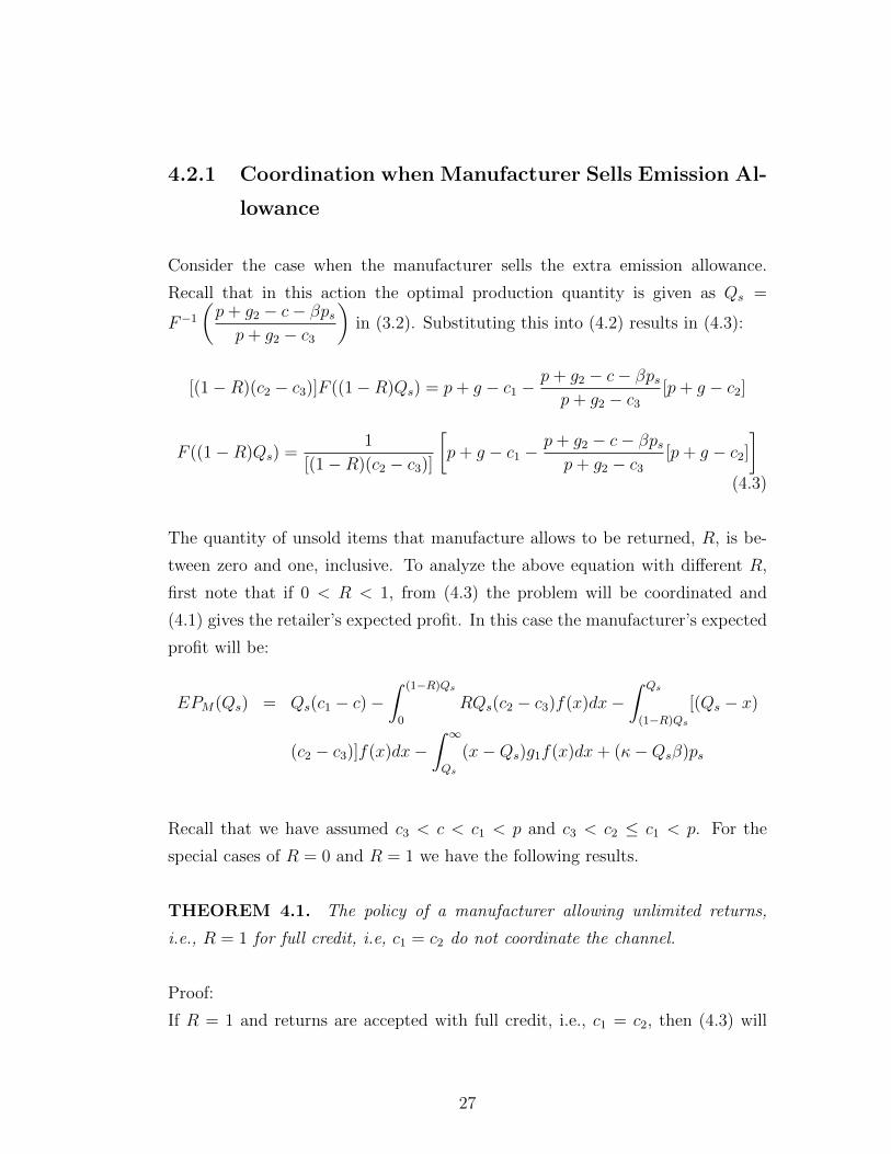
4.2.1 Coordination when Manufacturer Sells Emission Al-

lowance

Consider the case when the manufacturer sells the extra emission allowance.

Recall that in this action the optimal production quantity is given as Qs =

F−1(p+ g2 − c− βpsp+ g2 − c3

)in (3.2). Substituting this into (4.2) results in (4.3):

[(1−R)(c2 − c3)]F ((1−R)Qs) = p+ g − c1 −p+ g2 − c− βpsp+ g2 − c3

[p+ g − c2]

F ((1−R)Qs) =1

[(1−R)(c2 − c3)]

[p+ g − c1 −

p+ g2 − c− βpsp+ g2 − c3

[p+ g − c2]]

(4.3)

The quantity of unsold items that manufacture allows to be returned, R, is be-

tween zero and one, inclusive. To analyze the above equation with different R,

first note that if 0 < R < 1, from (4.3) the problem will be coordinated and

(4.1) gives the retailer’s expected profit. In this case the manufacturer’s expected

profit will be:

EPM(Qs) = Qs(c1 − c)−∫ (1−R)Qs

0

RQs(c2 − c3)f(x)dx−∫ Qs

(1−R)Qs

[(Qs − x)

(c2 − c3)]f(x)dx−∫ ∞Qs

(x−Qs)g1f(x)dx+ (κ−Qsβ)ps

Recall that we have assumed c3 < c < c1 < p and c3 < c2 ≤ c1 < p. For the

special cases of R = 0 and R = 1 we have the following results.

THEOREM 4.1. The policy of a manufacturer allowing unlimited returns,

i.e., R = 1 for full credit, i.e, c1 = c2 do not coordinate the channel.

Proof:

If R = 1 and returns are accepted with full credit, i.e., c1 = c2, then (4.3) will

27

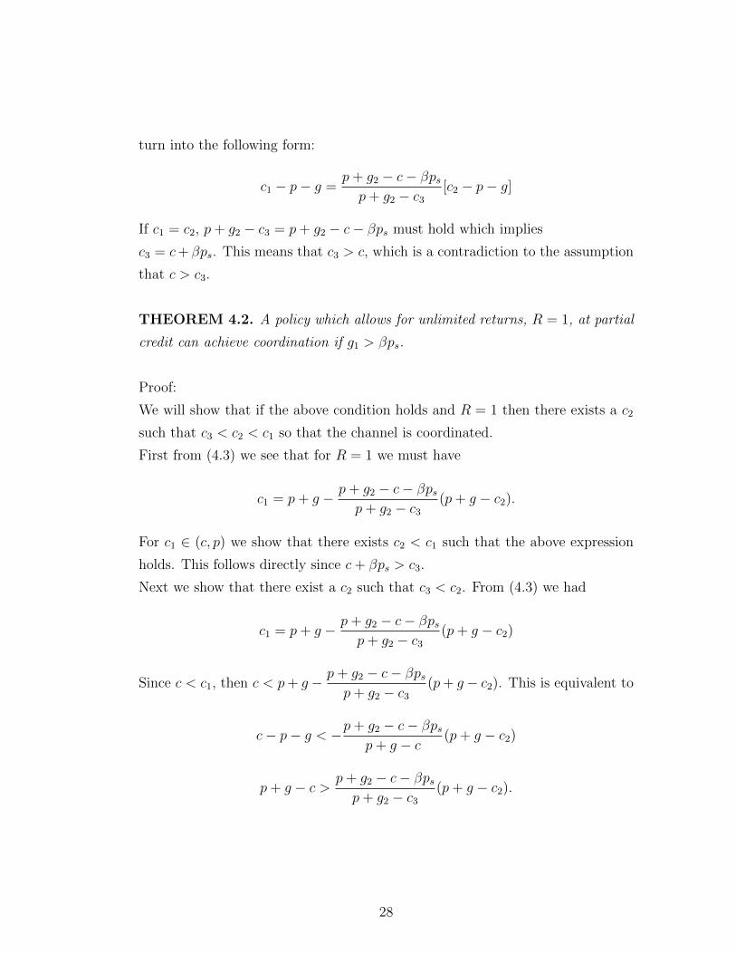
turn into the following form:

c1 − p− g =p+ g2 − c− βpsp+ g2 − c3

[c2 − p− g]

If c1 = c2, p+ g2 − c3 = p+ g2 − c− βps must hold which implies

c3 = c+ βps. This means that c3 > c, which is a contradiction to the assumption

that c > c3.

THEOREM 4.2. A policy which allows for unlimited returns, R = 1, at partial

credit can achieve coordination if g1 > βps.

Proof:

We will show that if the above condition holds and R = 1 then there exists a c2

such that c3 < c2 < c1 so that the channel is coordinated.

First from (4.3) we see that for R = 1 we must have

c1 = p+ g − p+ g2 − c− βpsp+ g2 − c3

(p+ g − c2).

For c1 ∈ (c, p) we show that there exists c2 < c1 such that the above expression

holds. This follows directly since c+ βps > c3.

Next we show that there exist a c2 such that c3 < c2. From (4.3) we had

c1 = p+ g − p+ g2 − c− βpsp+ g2 − c3

(p+ g − c2)

Since c < c1, then c < p+ g− p+ g2 − c− βpsp+ g2 − c3

(p+ g− c2). This is equivalent to

c− p− g < −p+ g2 − c− βpsp+ g − c

(p+ g − c2)

p+ g − c > p+ g2 − c− βpsp+ g2 − c3

(p+ g − c2).

28

If we assumep+ g2 − c− βps

p+ g − c> 1, then the following relation between both sides

of the equation must hold:

p+ g2 − c− βps > p+ g − c

g + g1 − c− βps > g − c

which is satisfied according to g1 > βps.

So assuming that g1 > βps appropriately chosen c1 and c2 for the following ex-

pression can achieve channel coordination.

THEOREM 4.3. The policy of a manufacturer allowing no returns, i.e., R = 0

coordinates the channel ifg1(c1 − c3)p+ g − c3

< βps holds.

Proof:

With R = 0, (4.3) will be

c1 = p+ g − p+ g2 − c− βpsp+ g2 − c3

[p+ g − c2]− (c2 − c3)F (Qs).

Substituting Qs given by (3.2) in the above formulation, we have

c1 = p+ g − p+ g2 − c− βpsp+ g2 − c3

[p+ g − c2]− (c2 − c3)p+ g2 − c− βpsp+ g2 − c3

(c1 − p− g)(p+ g2 − c3) = −(p+ g2 − c− βps)(p+ g − c3)

Given that g2 = g + g1, rewrite the above equation:

(c1 − p− g)(p+ g + g1 − c3) = −(p+ g + g1 − c− βps)(p+ g − c3)

Simplifying and rewriting this equation leads to the following steps:

(c1 − c) =g1(c1 − c3)(c3 − p− g)

+βps(c3 − p− g)

(c3 − p− g)

c1 = c−[g1(c1 − c3)p+ g − c3

− βps].

29

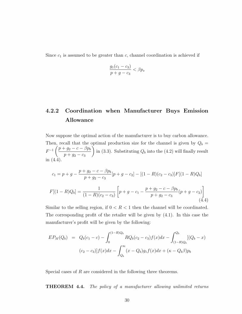
Since c1 is assumed to be greater than c, channel coordination is achieved if

g1(c1 − c3)p+ g − c3

< βps

4.2.2 Coordination when Manufacturer Buys Emission

Allowance

Now suppose the optimal action of the manufacturer is to buy carbon allowance.

Then, recall that the optimal production size for the channel is given by Qb =

F−1(p+ g2 − c− βpbp+ g2 − c3

)in (3.3). Substituting Qb into the (4.2) will finally result

in (4.4).

c1 = p+ g − p+ g2 − c− βpbp+ g2 − c3

[p+ g − c2]− [(1−R)(c2 − c3)]F [(1−R)Qb]

F [(1−R)Qb] =1

(1−R)(c2 − c3)

[p+ g − c1 −

p+ g2 − c− βpbp+ g2 − c3

(p+ g − c2)]

(4.4)

Similar to the selling region, if 0 < R < 1 then the channel will be coordinated.

The corresponding profit of the retailer will be given by (4.1). In this case the

manufacturer’s profit will be given by the following:

EPM(Qb) = Qb(c1 − c)−∫ (1−R)Qb

0

RQb(c2 − c3)f(x)dx−∫ Qb

(1−R)Qb

[(Qb − x)

(c2 − c3)]f(x)dx−∫ ∞Qb

(x−Qb)g1f(x)dx+ (κ−Qbβ)pb

Special cases of R are considered in the following three theorems.

THEOREM 4.4. The policy of a manufacturer allowing unlimited returns

30

(R = 1) for full credit (c1 = c2) is not optimal.

Proof: If R = 1 and return policy is full credit c1 = c2, then from (4.4) we

have

c1 − p− g =p+ g2 − c− βpbp+ g2 − c3

[c2 − p− g]

Since c1 = c2, then p + g2 − c3 = p + g2 − c− βpb. However this requires c3 > c,

which is a contradiction to the assumption that c > c3.

THEOREM 4.5. A policy which allows for unlimited returns at partial credit

is system optimal if g1 > βpb.

Proof:

We will show that if the above condition holds and R = 1, then there exists a c2

such that c3 < c2 < c1 so that the channel is coordinated.

First Substituting R = 1 into (4.4) will result in

c1 = p+ g − p+ g2 − c− βpbp+ g2 − c3

(p+ g − c2)

For c1 ∈ (c, p) we show that there exists c2 < c1 such that the above expression

holds. This follows directly since c+ βpb > c3.

Now we need to show that there exist a c2 such that c3 < c2. Since c < c1, then

c < p+ g − p+ g2 − c− βpbp+ g2 − c3

(p+ g − c2).

Or p+g−c > p+ g2 − c− βpbp+ g2 − c3

(p+g−c2), which is satisfied according to g1 > βpb.

THEOREM 4.6. The policy of a manufacturer allowing no returns i.e R = 0

is optimal ifg1(c1 − c3)p+ g − c3

< βpb

Proof:

31

From (4.4) we have

c1 − p− g = −p+ g2 − c− βpbp+ g2 − c3

[p+ g − c3]

Given that g2 = g + g1

(c1 − p− g)(c3 − p− g − g1) = (c+ βpb − p− g − g1)(c3 − p− g)

Rewriting the above equation results in

c1 = c−[g1(c1 − c3)p+ g − c3

− βpb]

Which implies that in order to achieve channel coordination the following condi-

tion must be satisfied.g1(c1 − c3)p+ g − c3

< βpb

4.2.3 Coordination when Optimal Order is κ/β

Substituting F

(κ

β

)into (4.2) results in

−c1 + p+ g − F(κ

β

)[p+ g − c2]− [(1−R)(c2 − c3)]F

[(1−R)

κ

β

]= 0

Rewriting it

[(1−R)(c2 − c3)]F[(1−R)

κ

β

]= p+ g − c1 − F

(κ

β

)[p+ g − c2]

= (p+ g)(1− F(κ

β

))− c1(1− F

(κ

β

)c2)

(4.5)

32

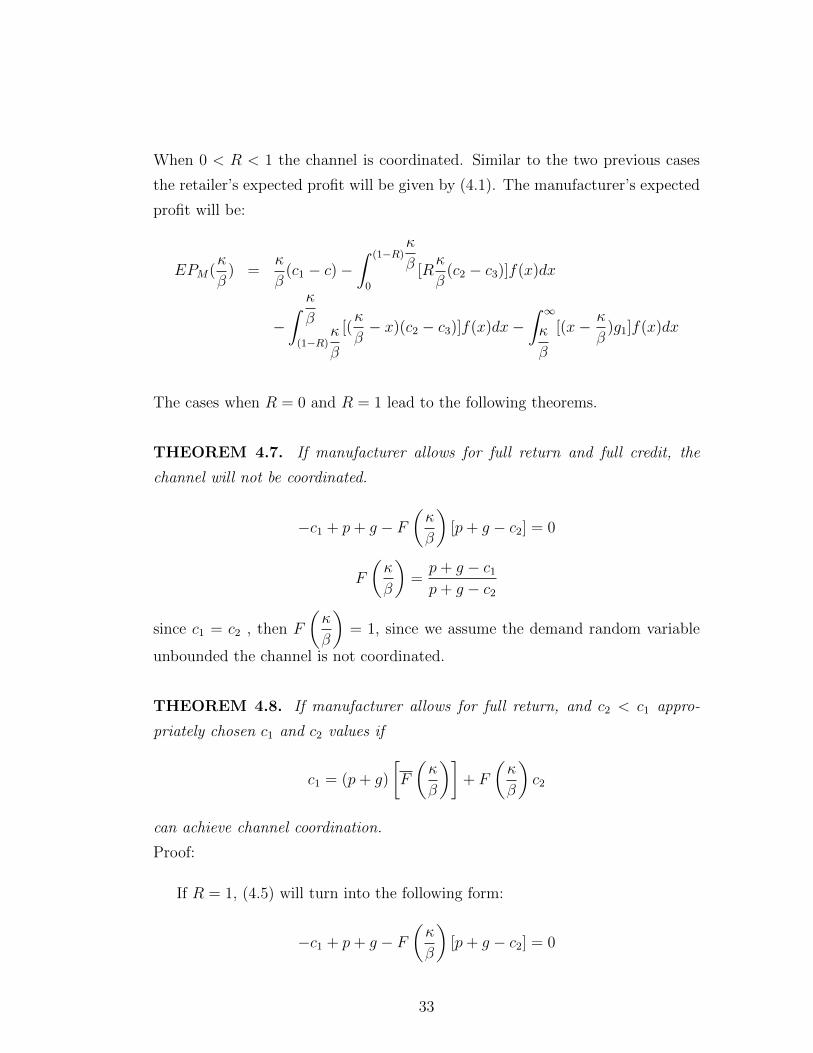
When 0 < R < 1 the channel is coordinated. Similar to the two previous cases

the retailer’s expected profit will be given by (4.1). The manufacturer’s expected

profit will be:

EPM(κ

β) =

κ

β(c1 − c)−

∫ (1−R)κ

β

0

[Rκ

β(c2 − c3)]f(x)dx

−∫ κ

β

(1−R)κ

β

[(κ

β− x)(c2 − c3)]f(x)dx−

∫ ∞κ

β

[(x− κ

β)g1]f(x)dx

The cases when R = 0 and R = 1 lead to the following theorems.

THEOREM 4.7. If manufacturer allows for full return and full credit, the

channel will not be coordinated.

−c1 + p+ g − F(κ

β

)[p+ g − c2] = 0

F

(κ

β

)=p+ g − c1p+ g − c2

since c1 = c2 , then F

(κ

β

)= 1, since we assume the demand random variable

unbounded the channel is not coordinated.

THEOREM 4.8. If manufacturer allows for full return, and c2 < c1 appro-

priately chosen c1 and c2 values if

c1 = (p+ g)

[F

(κ

β

)]+ F

(κ

β

)c2

can achieve channel coordination.

Proof:

If R = 1, (4.5) will turn into the following form:

−c1 + p+ g − F(κ

β

)[p+ g − c2] = 0

33

rewriting it will lead to

c1 = (p+ g)

[F

(κ

β

)]+ F

(κ

β

)c2

THEOREM 4.9. If manufacturer allows for no returns, channel is coordinated

if c1 = p+ g − (p+ g − c3)F(κ

β

)Proof:

If R = 0, (4.5) will turn to:

c1 = (p+ g)

[F

(κ

β

)]+ c3F

(κ

β

)From the above derivation, it is possible to check the retail pricing policy c1 for

the given κ.

F

(κ

β

)=p+ g − c1p+ g − c3

34

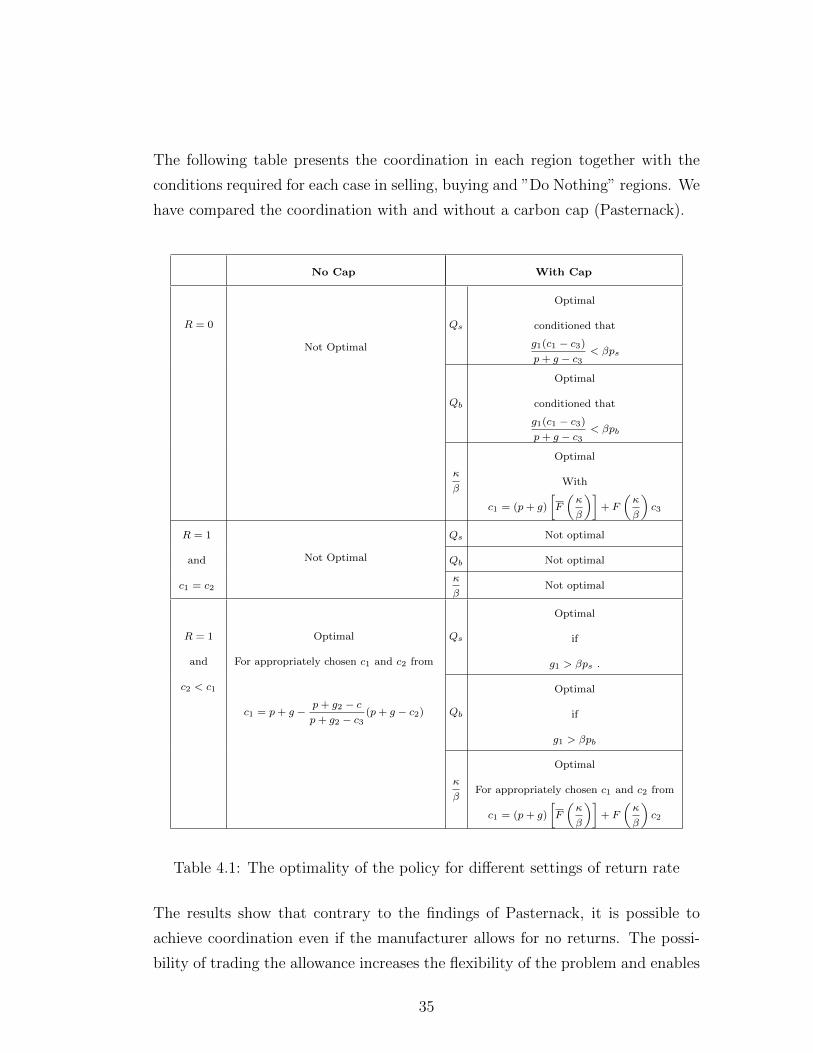
The following table presents the coordination in each region together with the

conditions required for each case in selling, buying and ”Do Nothing” regions. We

have compared the coordination with and without a carbon cap (Pasternack).

No Cap With Cap

R = 0

Not Optimal

Qs

Optimal

conditioned that

g1(c1 − c3)p+ g − c3

< βps

Qb

Optimal

conditioned that

g1(c1 − c3)p+ g − c3

< βpb

κ

β

Optimal

With

c1 = (p+ g)

[F

(κ

β

)]+ F

(κ

β

)c3

R = 1

and

c1 = c2

Not Optimal

Qs Not optimal

Qb Not optimal

κ

βNot optimal

R = 1

and

c2 < c1

Optimal

For appropriately chosen c1 and c2 from

c1 = p+ g −p+ g2 − cp+ g2 − c3

(p+ g − c2)

Qs

Optimal

if

g1 > βps .

Qb

Optimal

if

g1 > βpb

κ

β

Optimal

For appropriately chosen c1 and c2 from

c1 = (p+ g)

[F

(κ

β

)]+ F

(κ

β

)c2

Table 4.1: The optimality of the policy for different settings of return rate

The results show that contrary to the findings of Pasternack, it is possible to

achieve coordination even if the manufacturer allows for no returns. The possi-

bility of trading the allowance increases the flexibility of the problem and enables

35

the manufacturer to have more options in pricing policies, in the sense that while

the manufacturer allows for no returns, he can reduce the wholesale price in or-

der to motivate the retailer for the channel optimal ordering policy. Our findings

show that for the special cases of wholesale price the corresponding profit of both

parties can be increase after the coordination practice. This can be seen in our

numerical results.

When full returns for full credit is allowed, manufacturer is always the losing

part. In this case for the finite number of order quantities the coordination is not

achievable.

Similar to the results of Pasternack, when full returns with a return price less

than the wholesale price is allowed the manufacturer and retailer can have the

same order size. For the selling and buying cases of emission allowance, the con-

dition on the goodwill cost of manufacturer implies that for one unit of emission

per production, the cost of one unit of unsatisfied demand is larger than the

profit/cost of selling/buying one unit of emission allowance.

36

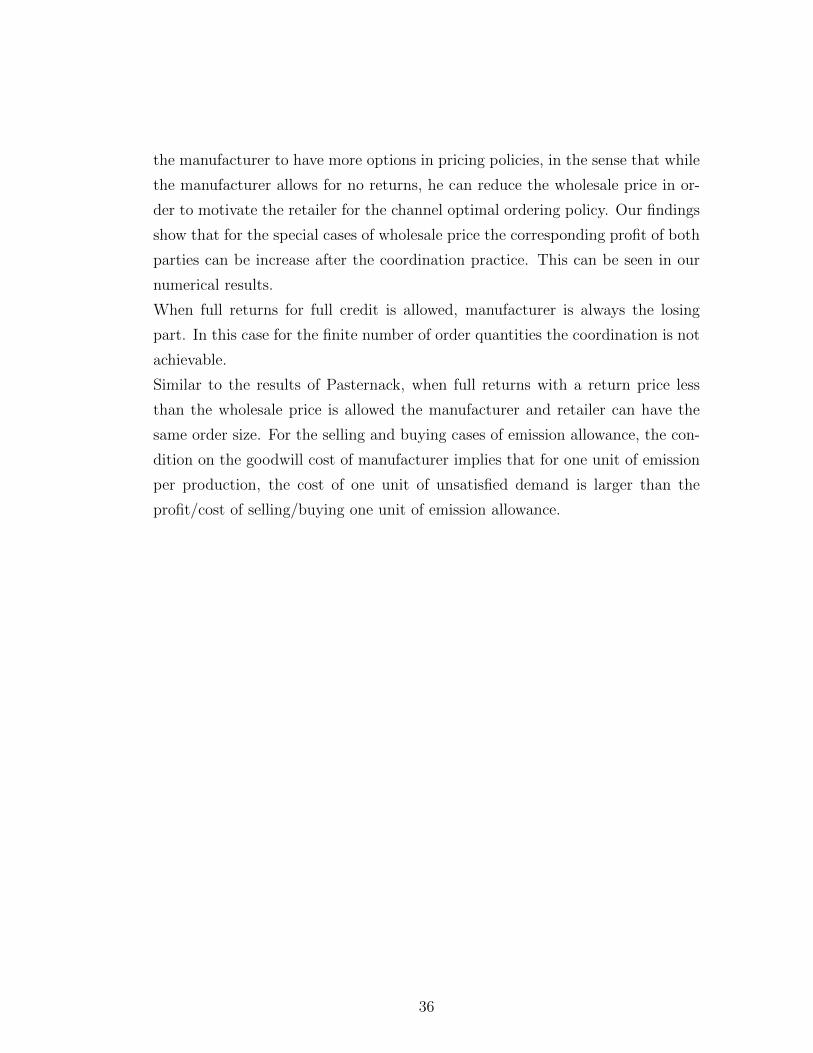
4.3 Numerical Analysis

In this chapter, we present a set of computational experiments in which we eval-

uate the optimal policies for the return contract and discuss the sensitivity of the

optimal policy parameters with respect to various system parameters. Suppose

that the end customer demand follows a normal distribution with mean 400 and

standard deviation of 100 units.

c = 1.5 g = 1.2 N(µ, σ) = N(400, 100) p = 4.5c1 = 3 g1 = 1.1 R = 0, 1 pb = 1c3 = 0.5 g2 = 2.3 β = 1 ps = 0.7

Table 4.2: Input Data for The Return Contract

When R = 0 and the retailer is profit maximizer (before coordination), we can

find the retailer’s optimal production quantity: Q∗R

−c1 + p+ g − F (Q∗R)(p+ g − c2)− F ((1−R)Q∗R)[(1−R)(c2 − c3)] = 0

which results in F (Q∗R) = 0.519., and the corresponding z value will be z = 0.05.

z =Q∗R − µ

σ. Therefore Q∗R = 405. The expected profit of the retailer with his

optimal order quantity will be: EPR(405) = 392.78. To specify the expected

profit of the manufacturer when retailer orders 405, first the κ value must be de-

clared. Because if the assigned cap is less than the retailer’s order, 405 units, then

the manufacturer must purchase the shortage from the market. Obviously β = 1

means that one unit of κ corresponds to one unit production. Suppose there

is no cap on the emission amount by manufacturer. That is, the manufacturer

can produce any order quantity which is placed by the retailer(In this case 405).

Then, regardless of the loss or profit incurred due to the cap, the manufacturer’s

expected profit will be: EPM(405) = 566.3.

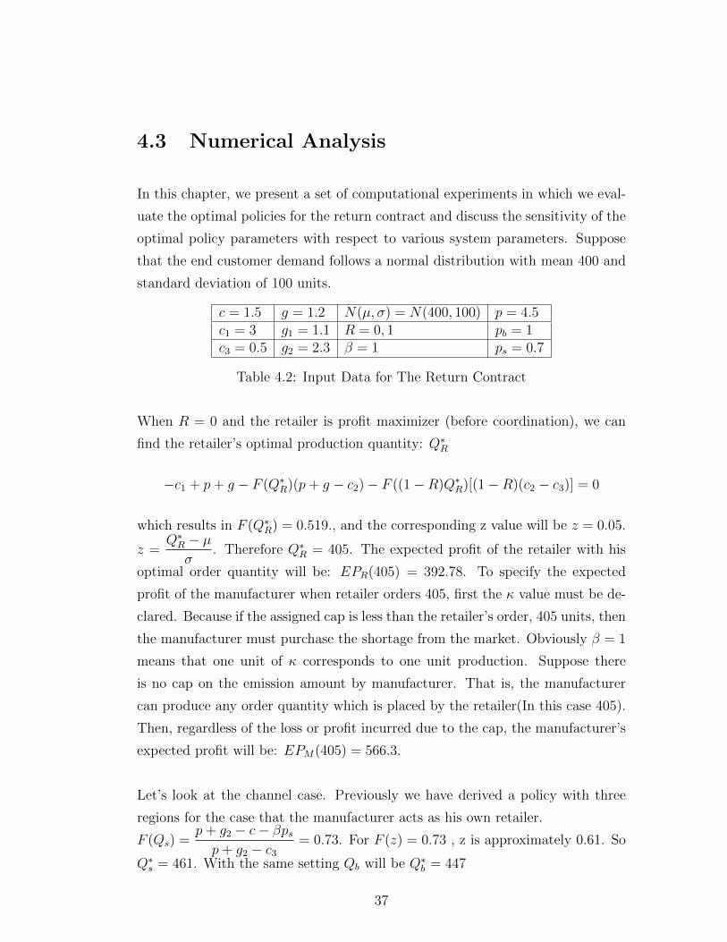
Let’s look at the channel case. Previously we have derived a policy with three

regions for the case that the manufacturer acts as his own retailer.

F (Qs) =p+ g2 − c− βpsp+ g2 − c3

= 0.73. For F (z) = 0.73 , z is approximately 0.61. So

Q∗s = 461. With the same setting Qb will be Q∗b = 447

37

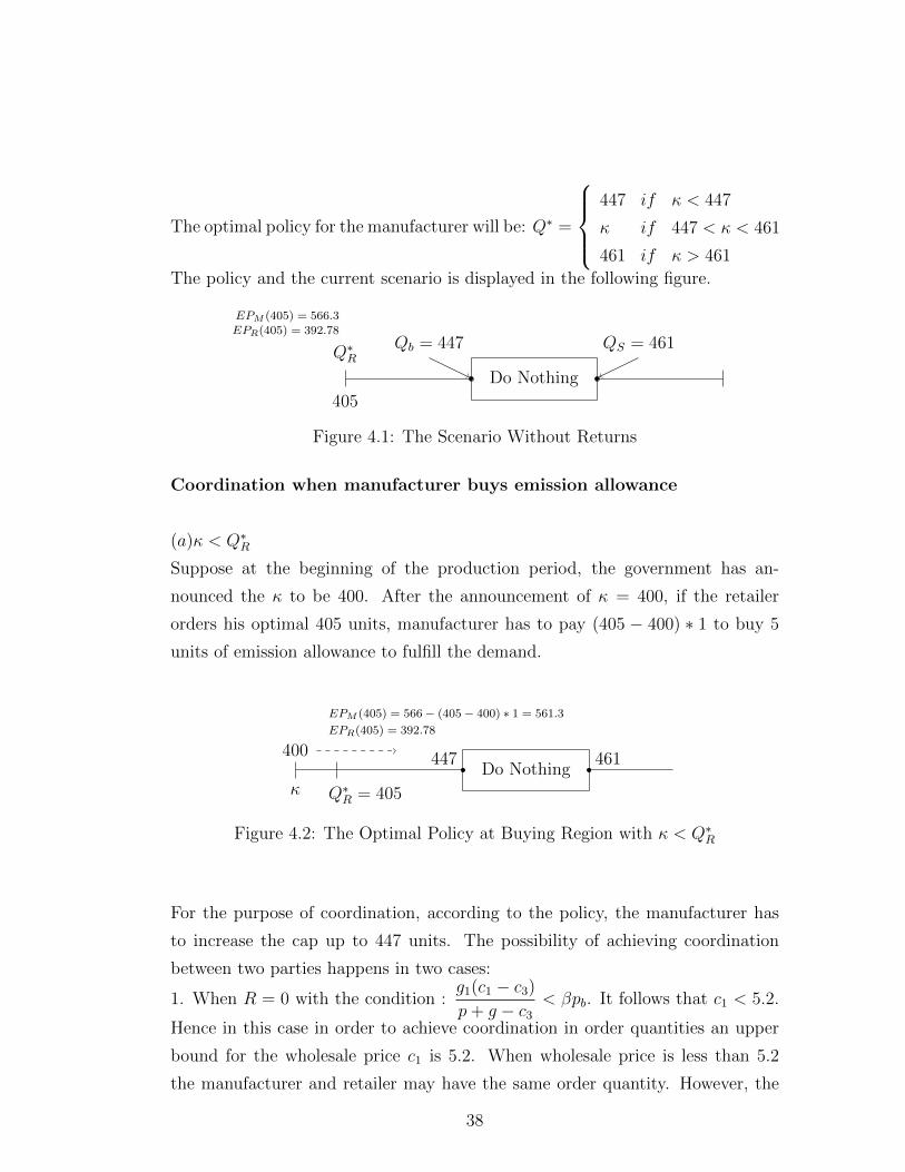
The optimal policy for the manufacturer will be: Q∗ =

447 if κ < 447

κ if 447 < κ < 461

461 if κ > 461

The policy and the current scenario is displayed in the following figure.

Do Nothing

Qb = 447 QS = 461Q∗R

405

EPR(405) = 392.78EPM (405) = 566.3

Figure 4.1: The Scenario Without Returns

Coordination when manufacturer buys emission allowance

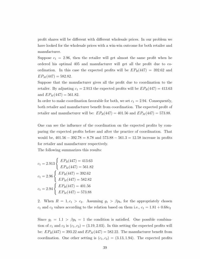
(a)κ < Q∗R

Suppose at the beginning of the production period, the government has an-

nounced the κ to be 400. After the announcement of κ = 400, if the retailer

orders his optimal 405 units, manufacturer has to pay (405 − 400) ∗ 1 to buy 5

units of emission allowance to fulfill the demand.

Do Nothing447 461

κ

400

Q∗R = 405

EPR(405) = 392.78

EPM (405) = 566− (405− 400) ∗ 1 = 561.3

Figure 4.2: The Optimal Policy at Buying Region with κ < Q∗R

For the purpose of coordination, according to the policy, the manufacturer has

to increase the cap up to 447 units. The possibility of achieving coordination

between two parties happens in two cases:

1. When R = 0 with the condition :g1(c1 − c3)p+ g − c3

< βpb. It follows that c1 < 5.2.

Hence in this case in order to achieve coordination in order quantities an upper

bound for the wholesale price c1 is 5.2. When wholesale price is less than 5.2

the manufacturer and retailer may have the same order quantity. However, the

38

profit shares will be different with different wholesale prices. In our problem we

have looked for the wholesale prices with a win-win outcome for both retailer and

manufacturer.

Suppose c1 = 2.96, then the retailer will get almost the same profit when he

ordered his optimal 405 and manufacturer will get all the profit due to co-

ordination. In this case the expected profits will be EPR(447) = 392.62 and

EPM(447) = 582.82.

Suppose that the manufacturer gives all the profit due to coordination to the

retailer. By adjusting c1 = 2.913 the expected profits will be EPR(447) = 413.63

and EPM(447) = 561.82.

In order to make coordination favorable for both, we set c1 = 2.94. Consequently,

both retailer and manufacturer benefit from coordination. The expected profit of

retailer and manufacturer will be: EPR(447) = 401.56 and EPM(447) = 573.88.

One can see the influence of the coordination on the expected profits by com-

paring the expected profits before and after the practice of coordination. That

would be, 401.56 − 392.78 = 8.78 and 573.88 − 561.3 = 12.58 increase in profits

for retailer and manufacturer respectively.

The following summarizes this results:

c1 = 2.913

{EPR(447) = 413.63

EPM(447) = 561.82

c1 = 2.96

{EPR(447) = 392.62

EPM(447) = 582.82

c1 = 2.94

{EPR(447) = 401.56

EPM(447) = 573.88

2. When R = 1, c1 > c2. Assuming g1 > βpb, for the appropriately chosen

c1 and c2 values according to the relation based on them i.e., c1 = 1.81 + 0.68c2

Since g1 = 1.1 > βpb = 1 the condition is satisfied. One possible combina-

tion of c1 and c2 is (c1, c2) = (3.19, 2.03). In this setting the expected profits will

be: EPR(447) = 393.22 and EPM(447) = 582.22. The manufacturer benefit from

coordination. One other setting is (c1, c2) = (3.13, 1.94). The expected profits

39

will be: EPR(447) = 414.13 and EPM(447) = 561.32. In which the retailer takes

all the profit of coordination. To make them both benefit from coordination, con-

sider (c1, c2) = (3.1632, 1.99). The expected profits will be: EPR(447) = 402.67

and EPM(447) = 572.77. The increase in expected profits compared to the un-

coordinated case will be 9.89 and 11.47 for retailer and manufacturer respectively.

The results are summarized as follows(after rounding to two digit decimals):

(c1, c2) = (3.13, 1.94)

{EPR(447) = 414.13

EPM(447) = 561.32

(c1, c2) = (3.19, 2.03)

{EPR(447) = 393.22

EPM(447) = 582.22

(c1, c2) = (3.16, 1.99)

{EPR(447) = 402.67

EPM(447) = 572.77

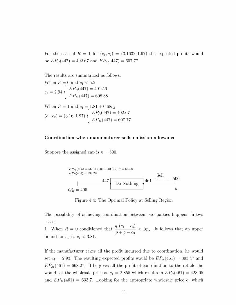
(b) Q∗R < κ

The carbon cap κ could also be larger than 405, say 435 units. In this case,

the retailer’s profit does not change. However, when the independent retailer

orders his optimal 405 units, the manufacturer could sell the extra (435 − 405)

units with ps = 0.7 and produce retailer’s optimal order. This case refers to

uncoordinated system and the expected profits will be: EPR(447) = 392.78 and

EPm(447) = 566.3 + 21 = 587.3.

Do Nothing447 461

Q∗R = 405

435

κ

EPR(405) = 392.78

EPM (405) = 566 + (435− 405) ∗ 0.7 = 587.3

Figure 4.3: The Optimal Policy at Buying Region with Q∗R < κ

When coordination is applied, the objective of both manufacturer and retailer

would be 447 units. For the case of R = 0 if c1 = 2.94 is accepted, the expected

profits would be EPR(447) = 401.56 and EPm(447) = 608.88. Again an increase

in both of the expected profits compared to the uncoordinated model is observed.

40

For the case of R = 1 for (c1, c2) = (3.1632, 1.97) the expected profits would

be EPR(447) = 402.67 and EPM(447) = 607.77.

The results are summarized as follows:

When R = 0 and c1 < 5.2

c1 = 2.94

{EPR(447) = 401.56

EPM(447) = 608.88

When R = 1 and c1 = 1.81 + 0.68c2

(c1, c2) = (3.16, 1.97)

{EPR(447) = 402.67

EPM(447) = 607.77

Coordination when manufacturer sells emission allowance

Suppose the assigned cap is κ = 500,

Do Nothing

Sell447 461 500

κQ∗R = 405

EPR(405) = 392.78

EPM (405) = 566 + (500− 405) ∗ 0.7 = 632.8

Figure 4.4: The Optimal Policy at Selling Region

The possibility of achieving coordination between two parties happens in two

cases:

1. When R = 0 conditioned thatg1(c1 − c3)p+ g − c3

< βps. It follows that an upper

bound for c1 is: c1 < 3.81.

If the manufacturer takes all the profit incurred due to coordination, he would

set c1 = 2.93. The resulting expected profits would be EPR(461) = 393.47 and

EPM(461) = 668.27. If he gives all the profit of coordination to the retailer he

would set the wholesale price as c1 = 2.855 which results in EPR(461) = 428.05

and EPM(461) = 633.7. Looking for the appropriate wholesale price c1 which

41

could benefit both parties, we found: c1 = 2.88. The expected profit of retailer

and manufacturer will be: EPR(461) = 416.5 and EPM(461) = 645.22. The

additional profits after the coordination would be 645.22− 632.8 = 12.42 for the

manufacturer and 416.5− 392.78 = 23.72 for retailer.

Special cases which result in increase in profits are summarized as follows:

c1 = 2.93

{EPR(461) = 393.47

EPM(461) = 668.27

c1 = 2.85

{EPR(461) = 428

EPM(461) = 633.7

c1 = 2.88

{EPR(461) = 416.5

EPM(461) = 645.22

2. When R = 1, c1 > c2, assuming g1 > βps, then for the appropriately chosen c1

and c2 values according to the relation based on them i.e. c1 = 1.54 + 0.73c2 The

condition is satisfied since g1 = 1.1 > βps = 0.7

Suppose c2 = 2.326 and c1 = 3.24. The expected profits will be: EPR(461) =

393.1 and EPM(461) = 668.6. If c2 = 2.188 and c1 = 3.137, the expected profits

will be: EPR(461) = 429 and EPM(461) = 632.75.

Letting c2 = 2.25, then c1 = 3.182. In this setting the expected profits will be:

EPR(461) = 412.83 and EPM(461) = 648.9 . The additional profit due to coor-

dination will be 20.05 and 16.1 respectively.

The results are summarized as follows(after rounding to two digit decimals):

(c1, c2) = (3.24, 2.32)

{EPR(461) = 393.1

EPM(461) = 668.6

(c1, c2) = (3.13, 2.19)

{EPR(461) = 429

EPM(461) = 632.75

(c1, c2) = (3.18, 2.25)

{EPR(461) = 412.83

EPM(461) = 648.9

Remark: What if the parties do not act as what policy suggests? to answer

42

this question we consider the above case. With κ = 500 they have to accept

Qs = 461 as the optimal. Suppose they agree on Qb = 447 which is the optimal

for the channel but in buying region. Intuitively we can find a c1 which results in

coordination with increase in expected profits with respect to the retailer’s opti-

mal order Q∗R. However the increase would be less than the case when they accept

461. To see this case in details, we proceed with a coordinating c1 = 2.91. For 447

units the expected profits will be EPR(447) = 414.97 and EPM(447) = 644.57.

c1 = 2.91

{EPR(447) = 414.97

EPM(447) = 644.57

for which the overall profit is EPR(447) + EPM(447) = 1059.55. However the

overall profit with 461 units is 416.5 + 645.22 = 1061.72.

If they act based on a order size even less than 447 units, the overall channel

profit will decrease accordingly. For instance, ordering 420 units will result in

1042.64 overall channel profit for c1 = 2.96

c1 = 2.96

{EPR(420) = 407.21

EPM(420) = 635.44

If they agree on 500 units, with c1 = 2.8, expected profits will be EPR(500) =

406.67 and EPM(500) = 640.83. The overall profit will be 406.67 + 640.83 =

1047.5.

c1 = 2.8

{EPR(500) = 406.67

EPM(500) = 640.83

Coordination when quantity ordered is in κ/β region

Suppose the assigned κ is 455.

43

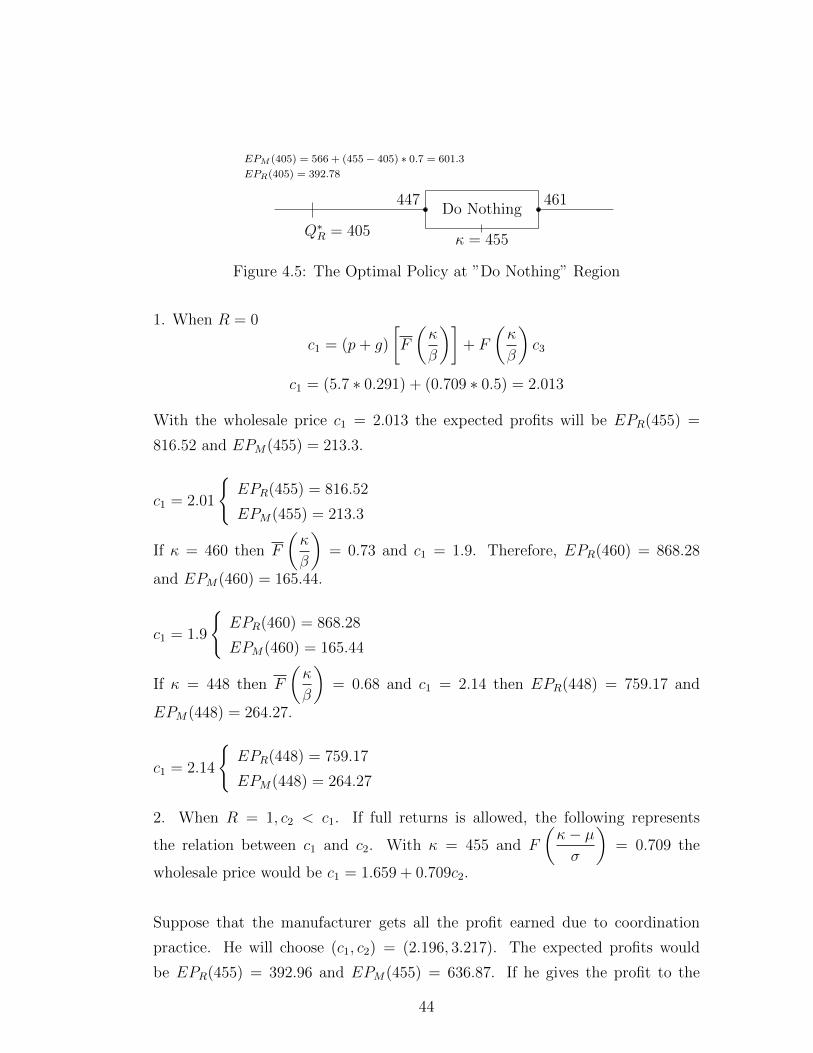
Do Nothing447 461

κ = 455Q∗R = 405

EPR(405) = 392.78

EPM (405) = 566 + (455− 405) ∗ 0.7 = 601.3

Figure 4.5: The Optimal Policy at ”Do Nothing” Region

1. When R = 0

c1 = (p+ g)

[F

(κ

β

)]+ F

(κ

β

)c3

c1 = (5.7 ∗ 0.291) + (0.709 ∗ 0.5) = 2.013

With the wholesale price c1 = 2.013 the expected profits will be EPR(455) =

816.52 and EPM(455) = 213.3.

c1 = 2.01

{EPR(455) = 816.52

EPM(455) = 213.3

If κ = 460 then F

(κ

β

)= 0.73 and c1 = 1.9. Therefore, EPR(460) = 868.28

and EPM(460) = 165.44.

c1 = 1.9

{EPR(460) = 868.28

EPM(460) = 165.44

If κ = 448 then F

(κ

β

)= 0.68 and c1 = 2.14 then EPR(448) = 759.17 and

EPM(448) = 264.27.

c1 = 2.14

{EPR(448) = 759.17

EPM(448) = 264.27

2. When R = 1, c2 < c1. If full returns is allowed, the following represents

the relation between c1 and c2. With κ = 455 and F

(κ− µσ

)= 0.709 the

wholesale price would be c1 = 1.659 + 0.709c2.

Suppose that the manufacturer gets all the profit earned due to coordination

practice. He will choose (c1, c2) = (2.196, 3.217). The expected profits would

be EPR(455) = 392.96 and EPM(455) = 636.87. If he gives the profit to the

44

retailer, then (c1, c2) = (2.055, 3.117). Therefore, the expected profits would be

EPR(455) = 428.13 and EPM(455) = 601.7

One middle road strategy is to choose c1 and c2 such that both will benefit from

coordination. For this purpose, the manufacturer sets (c1, c2) = (2.125, 3.166) .

Then EPR(455) = 410.96 and EPM(455) = 618.86

The results are summarized as follows(after rounding to two digit decimals):

(c1, c2) = (3.21, 2.19)

{EPR(455) = 392.96

EPM(455) = 636.87

(c1, c2) = (3.12, 2.05)

{EPR(455) = 428.13

EPM(455) = 601.7

(c1, c2) = (3.17, 2.12)

{EPR(455) = 410.96

EPM(455) = 618.86

Profit Shares Of the Manufacturer and the Retailer

Let

PSb =EPR(447)

EPR(447) + EPM(447)

PSs =EPR(461)

EPR(461) + EPM(461)

PSn =EPR(455)

EPR(455) + EPM(455)

represent the profit share of retailer from the total channel profit when the order

quantity falls within Qb, Qs and ”Do Nothing” regions respectively.

When R = 0,

PSb =401.56

401.56 + 573.88=

401.56

975.44= 0.411

PSs =416.5

416.5 + 645.22=

416.5

1061.72= 0.392

45

PSn =816.52

816.52 + 213.3=

816.52

1029.82= 0.793

When R = 1,

PSb =402.67

402.67 + 572.77=

402.67

975.44= 0.413

PSs =412.83

412.83 + 648.9=

412.83

1061.73= 0.389

PSn =410.96

410.96 + 618.86=

410.96

1029.82= 0.399

It is observed that in every case except when in ”Do Nothing” region the man-

ufacturer allows no returns, the profit share of retailer would be approximately

40%. It is also interesting to make a comparison with the case when the retailer

orders his optimal. In buying region for instance, the proportion of profit incurred

by retailer is 0.411. Coordination increased his profit but no changes happened

in the profit share. In selling region this would be 0.383. In case when κ is in

between, the proportion of retailer’s profit to the total under retailer’s optimal

is 0.395. So the majority of the cases suggest that it is favorable for retailer to

accept coordination.

46

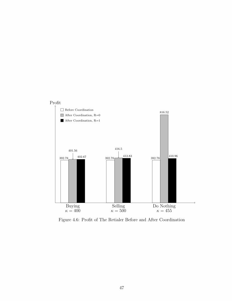
Buyingκ = 400

392.78 402.67

401.56

Sellingκ = 500

392.78412.83

416.5

Do Nothingκ = 455

392.78

816.52

410.96

Before Coordination

After Coordination, R=0

After Coordination, R=1

Profit

Figure 4.6: Profit of The Retialer Before and After Coordination

47

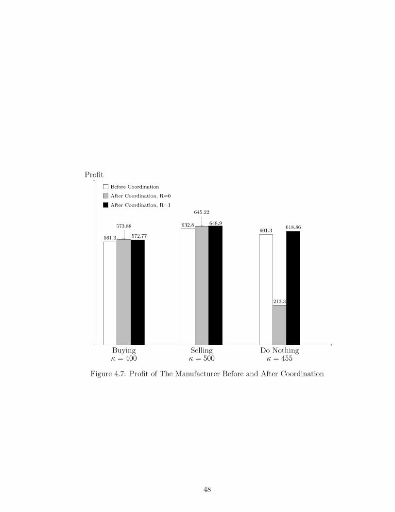
Profit

Buyingκ = 400

561.3 572.77

573.88

Sellingκ = 500

632.8 648.9

645.22

Do Nothingκ = 455

601.3

213.3

618.86

Before Coordination

After Coordination, R=0

After Coordination, R=1

Figure 4.7: Profit of The Manufacturer Before and After Coordination

48

Chapter 5

Coordination Under Rebate

Contract

Introduction

In this chapter, we show that a policy that combines the use of wholesale price

and channel rebate for the sales beyond a pre-determined amount coordinates a

channel composed of a retailer and a manufacturer where the manufacturer is

exposed to restrictions on the amount of carbon emission with trading option.

According to the rebate contract, the manufacturer pays the retailer a predeter-

mined credit u for the sales beyond a predetermined target quantity of T . We

assume that the goodwill cost associated with unsatisfied demand is negligible.

Therefore the order quantities in each case of buying and selling carbon allowance

will have the following form:

Qb = F−1(p− c− βpbp− c3

)(5.1)

Qs = F−1(p− c− βpsp− c3

)(5.2)

The Independent Retailer Without Rebate:

49

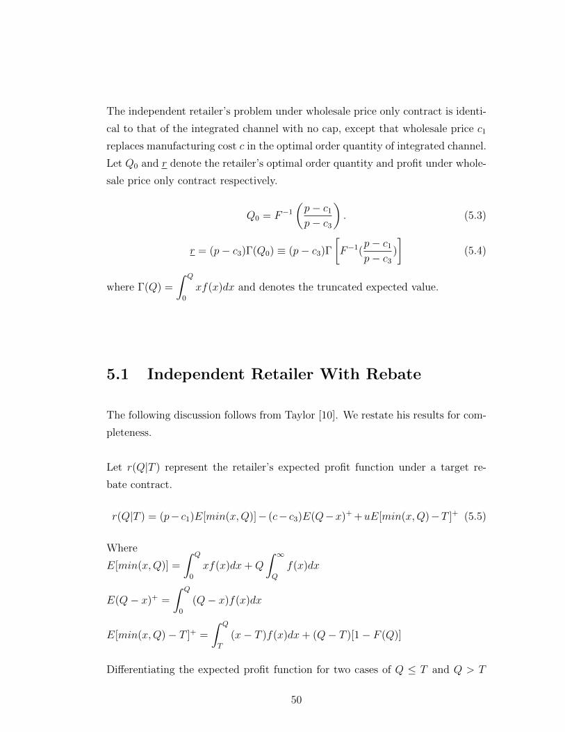
The independent retailer’s problem under wholesale price only contract is identi-

cal to that of the integrated channel with no cap, except that wholesale price c1

replaces manufacturing cost c in the optimal order quantity of integrated channel.

Let Q0 and r denote the retailer’s optimal order quantity and profit under whole-

sale price only contract respectively.

Q0 = F−1(p− c1p− c3

). (5.3)

r = (p− c3)Γ(Q0) ≡ (p− c3)Γ[F−1(

p− c1p− c3

)

](5.4)

where Γ(Q) =

∫ Q

0

xf(x)dx and denotes the truncated expected value.

5.1 Independent Retailer With Rebate

The following discussion follows from Taylor [10]. We restate his results for com-

pleteness.

Let r(Q|T ) represent the retailer’s expected profit function under a target re-

bate contract.

r(Q|T ) = (p− c1)E[min(x,Q)]− (c− c3)E(Q−x)+ +uE[min(x,Q)−T ]+ (5.5)

Where

E[min(x,Q)] =

∫ Q

0

xf(x)dx+Q

∫ ∞Q

f(x)dx

E(Q− x)+ =

∫ Q

0

(Q− x)f(x)dx

E[min(x,Q)− T ]+ =

∫ Q

T

(x− T )f(x)dx+ (Q− T )[1− F (Q)]

Differentiating the expected profit function for two cases of Q ≤ T and Q > T

50

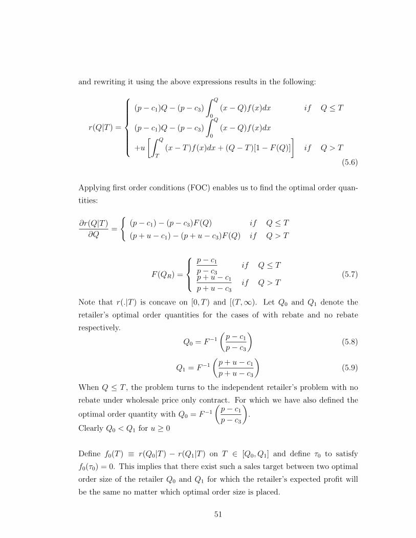
and rewriting it using the above expressions results in the following:

r(Q|T ) =

(p− c1)Q− (p− c3)∫ Q

0

(x−Q)f(x)dx if Q ≤ T

(p− c1)Q− (p− c3)∫ Q

0

(x−Q)f(x)dx

+u

[∫ Q

T

(x− T )f(x)dx+ (Q− T )[1− F (Q)]

]if Q > T

(5.6)

Applying first order conditions (FOC) enables us to find the optimal order quan-

tities:

∂r(Q|T )

∂Q=

{(p− c1)− (p− c3)F (Q) if Q ≤ T

(p+ u− c1)− (p+ u− c3)F (Q) if Q > T

F (QR) =

p− c1p− c3

if Q ≤ T

p+ u− c1p+ u− c3

if Q > T(5.7)

Note that r(.|T ) is concave on [0, T ) and [(T,∞). Let Q0 and Q1 denote the

retailer’s optimal order quantities for the cases of with rebate and no rebate

respectively.

Q0 = F−1(p− c1p− c3

)(5.8)

Q1 = F−1(p+ u− c1p+ u− c3

)(5.9)

When Q ≤ T , the problem turns to the independent retailer’s problem with no

rebate under wholesale price only contract. For which we have also defined the

optimal order quantity with Q0 = F−1(p− c1p− c3

).

Clearly Q0 < Q1 for u ≥ 0

Define f0(T ) ≡ r(Q0|T ) − r(Q1|T ) on T ∈ [Q0, Q1] and define τ0 to satisfy

f0(τ0) = 0. This implies that there exist such a sales target between two optimal

order size of the retailer Q0 and Q1 for which the retailer’s expected profit will

be the same no matter which optimal order size is placed.

51

Theorem 5.1. (a) τ0 exists, is unique, and satisfies τ0 ∈ (Q0, Q1)

(b) The optimal ordering policy for the retailer under a target rebate, Q∗R, is given

by the following:

Q∗R =

Q1 if T < τ0

Q0 if T > τ0

{Q0, Q1} if T = τ0

(5.10)

Proof from Taylor [10]:

It is straightforward to show that if T ≤ Q0, then Q1 maximizes r(.|T ) and if

T ≥ Q1, then Q0 maximizes the r(.|T ).

If Q0 ≤ T ≤ Q1, then r(Q0|T ) = (p− c3)Γ(Q0) and r(Q1|T ) = (p+u−s)Γ(Q1)−u[Γ(T ) + T (1 − F (T ))]. Because f0(Q0) < 0 < f0(Q1), and f0(.) is continuous

and increasing, there exist a singled valued inverse function f−10 and a unique

τ0; further, τ0 ∈ (Q0, Q1). If Q0 < T < Q1, then limQ→T−(∂/∂Q)r(Q|T ) < 0 <

limQ→T+(∂/∂Q)r(Q|T ). Because Q0 maximizes r(.|T ) on [0, T ) and Q1 maxi-

mizes r(.|T ) on (T,∞), then Q∗R = arg maxQ∈[Q0,Q1]r(Q|T ). If T < τ0, then

f0(T ) < 0 and r(Q1|T ) > r(Q0|T ). If T > τ0, then f0(T ) > 0.

Regarding the above theorem we have the following interpretations.

The retailer’s optimal order quantity Q∗R is decreasing in T. Consider the extreme

values of T. If T is extremely large, then the probability of selling units beyond

T is very small. To receive rebate, the retailer’s order size must be larger than T .

However, in such a case the resulting overage cost exceeds the expected revenue

from the rebate. As a consequent, the retailer behaves as if there exists no rebate

and orders the same quantity in the no rebate case. In other words he will order

Q0. If T = 0, then the the retailer receives p + u for each unit sell. However, in

this case the manufacturer will increase the retail price to compensate the loss.

Hence the optimal order quantity for the retailer will be the newsvendor quantity

where the retail price is p+ u, which is denoted by Q1.

For intermediate values of T, the retailer has to choose whether wants the rebate

i.e., orders more than T or not. In either case, the retailer’s optimal order quan-

tity is a function of expected cost and marginal revenue from an incremental sale.

52

If the retailer orders more than T, the marginal revenue is p + u; if he orders

less than T, the marginal revenue will be p. As T increases, the attractiveness

of going for the rebate decreases. At the threshold τ0 the retailer is indifferent

between ordering Q0 and Q1. (See Taylor [10])

The retailer profit under a target rebate is

r =

{(p+ u− s)Γ(Q1)− u[Γ(T ) + T (1− F (T ))] if T < τ0

(p− c3)Γ(Q0) if T ≥ τ0(5.11)

5.2 Channel Coordination

Recall that in order to achieve channel coordination the order quantity of two

parties must be equal. That is, the order quantity when the manufacturer acts

as there exists no retailer (with Qs, Qb and κ/β) with the case when there exists

an independent retailer (Q∗R) must be equal. In this part, we study the settings

for each of contract parameters, i.e., wholesale price c1, rebate u and target sales

T , that may lead to achieve coordination. Similar to the return contract we

have three cases: selling, buying the emission allowance and using all available

allowance that is ”Do Nothing” region.

5.2.1 Coordination when Manufacturer Sells Emission Al-

lowance

Let πs denote the channel’s profit corresponding to the optimal order quantity Qs.

Proposition 5.1. Let u∗s(c1) denote the optimal rebate amount in the selling

53

region. For any δ ∈ (0, πs), u∗s(c1) is set such that:

u∗s(c1) =(p− c3)(c1 − c− βps)

c+ βps − c3

Proof:

It follows from the first order condition for the case of Q > T , using F (Qs) =p− c− βpsp− c3

.

∂r(Q|T )

∂Q= (p+ u− c1)− (p+ u− c3)F (Qs) = 0

The optimal rebate amount is a function of wholesale price c1.

us(c1)− us(c1)F (Qs) = c1 − p+ (p− c3)F (Qs)

us(c1)[1− F (Qs)] = c1 − p+ (p− c3)F (Qs)

us(c1) =(c1 − p) + (p− c3)F (Qs)

F (Qs)

u∗s(c1) =(p− c3)(c1 − c− βps)

c+ βps − c3(5.12)

Remark.

The equation above represents the relation of two of the contract parameters,

namely wholesale price c1 and target rebate u. As the equation displays, the

target rebate is a function of the wholesale price. The equation, however does

not result in a single combination of c1 and u∗s(c1). Suppose the manufacturer

and retailer agree on a profit sharing structure. When the retailer is a profit

maximizer, he orders his optimal Q∗R, which amounts to the expected profit of

r. Suppose by adding ε to the retailer’s profit, the manufacturer increases the

retailer’s profit from the current value r to the agreed amount δ. Then (5.12) will

lead to a single c1, u∗s(c1) pair which will result in the above profit sharing.

Proposition 5.2. For any δ ∈ (0, πs), (a). The optimal wholesale price c∗1

54

is set such that:

(p− c3)Γ[F−1(

p− c1p− c3

)

]= δ − ε (5.13)

(b). The optimaal sales target is set such that:

(p+ u∗s − c3)Γ(Qs)− u∗s(Γ(T ∗) + T ∗(1− F (T ∗))) = δ (5.14)

Proof (a): It is straightforward. In order to realize δ as the new expected profit

of the retailer, c1 is the only contract parameter which influences the retailer’s

profit margin. Intuitively, one expects ca to be decreased if an increase in re-

tailer’s profit is expected.

Proof (b): It is straightforward. We mentioned that the manufacturer convinced

the retailer to set the channel optimal order quantity as his optimal. The re-

tailer agreed to the channel optimal Qs in return of an increase equal to ε in his

expected profit. With increase in profit his new expected profit will reach to δ.

As a consequent, T will be set such that the retailers profit under target rebate

will be δ. The left hand side of the equality sign refers to the expected profit of

retailer after rebate is realized from (5.11).

Corollary 5.1.

Under the coordinating contract parameters, the resulting profit to the manufac-

turer and retailer will be m∗s = πs − δ and r∗s = δ respectively.

5.2.2 Coordination when Manufacturer Buys Emission

Allowance

Let πb denote the channel’s profit with the optimal order quantity Qb.

Proposition 5.4. Let u∗b(c1) denote the optimal rebate amount in the buying

region. For any δ ∈ (0, πb), u∗b(c1) is set such that:

ub(c1) =(p− c3)(c1 − c− βpb)

c+ βpb − c3(5.15)

55

Proof is similar to the same case in selling region.

Proposition 5.5. For any δ ∈ (0, πb), (a). The optimal wholesale price c∗1

is set such that:

r = δ − ε (5.16)

(b). The optimal sales target is set such that:

(p+ u∗b − c3)Γ(Qb)− u∗b(Γ(T ∗) + T ∗(1− F (T ∗))) = δ (5.17)

Proofs are similar to the same case in selling region.

Corollary 5.2.

Under the coordinating contract parameters, the profit of manufacturer and re-

tailer will be m∗b = πb − δ and r∗b = δ Respectively.

5.2.3 Coordination when Manufacturer Produces κ/β

Units

Let πn denote the channel’s profit with the optimal order quantity κ/β.

Proposition 5.7. Let u∗n(c1) denote the optimal rebate amount in ”Do Noth-

ing” region. For any δ ∈ (0, πn), u∗n(c1) is set such that:

un(c1) =(p− c3)F (κ/β)(c1 − p)

F (κ/β)(5.18)

Proof is similar to the same case in selling region.

Proposition 5.8. For any δ ∈ (0, πn), (a). The optimal wholesale price c∗1

56

is set such that:

r = δ − ε (5.19)

(b). The optimal sales target is set such that:

(p+ u∗n − c3)Γ(κ/β)− u∗n(Γ(T ∗) + T ∗(1− F (T ∗))) = δ (5.20)

Proof is similar to the same case in selling region.

Corollary 5.3.

Under the coordinating contract parameters, the profit of manufacturer and re-

tailer will be m∗n = πn − δ and r∗n = δ respectively.

57

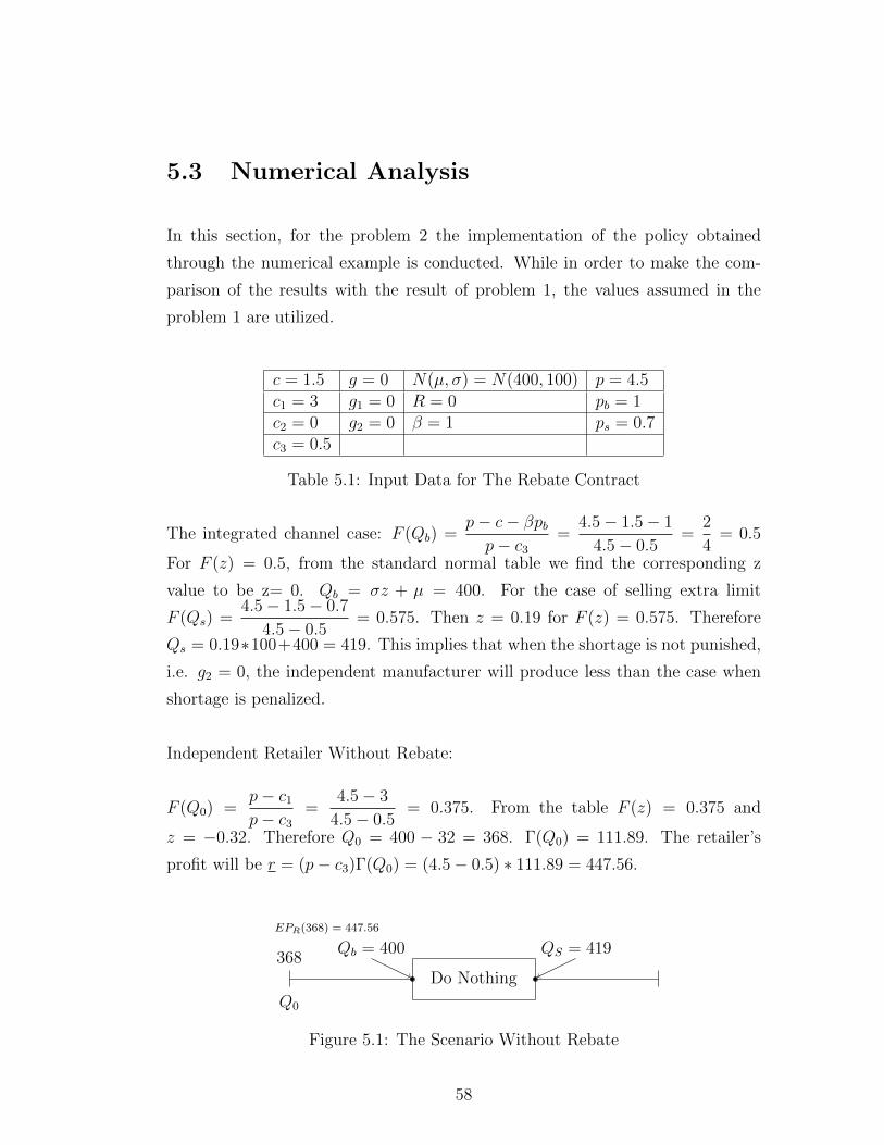
5.3 Numerical Analysis

In this section, for the problem 2 the implementation of the policy obtained

through the numerical example is conducted. While in order to make the com-

parison of the results with the result of problem 1, the values assumed in the

problem 1 are utilized.

c = 1.5 g = 0 N(µ, σ) = N(400, 100) p = 4.5c1 = 3 g1 = 0 R = 0 pb = 1c2 = 0 g2 = 0 β = 1 ps = 0.7c3 = 0.5

Table 5.1: Input Data for The Rebate Contract

The integrated channel case: F (Qb) =p− c− βpbp− c3

=4.5− 1.5− 1

4.5− 0.5=

2

4= 0.5

For F (z) = 0.5, from the standard normal table we find the corresponding z

value to be z= 0. Qb = σz + µ = 400. For the case of selling extra limit

F (Qs) =4.5− 1.5− 0.7

4.5− 0.5= 0.575. Then z = 0.19 for F (z) = 0.575. Therefore

Qs = 0.19∗100+400 = 419. This implies that when the shortage is not punished,

i.e. g2 = 0, the independent manufacturer will produce less than the case when

shortage is penalized.

Independent Retailer Without Rebate:

F (Q0) =p− c1p− c3

=4.5− 3

4.5− 0.5= 0.375. From the table F (z) = 0.375 and

z = −0.32. Therefore Q0 = 400 − 32 = 368. Γ(Q0) = 111.89. The retailer’s

profit will be r = (p− c3)Γ(Q0) = (4.5− 0.5) ∗ 111.89 = 447.56.

Do Nothing

Qb = 400 QS = 419368

Q0

EPR(368) = 447.56

Figure 5.1: The Scenario Without Rebate

58

Independent Retailer With Rebate:

Channel coordination requires the optimal order sizes of integrated channel and

independent retailer to be equal. Suppose the given κ = 450. Since κ > Qsβ. We

have to reduce the order quantity to 419 units. , We proceed to find the optimal

values for system parameters.

us(c1) =(p− c3)(c1 − c− βps)

c+ βps − c3=

(4.5− 0.5)(c1 − 1.5− 0.7)

1.5 + 0.7− 0.5= 2.35c1 − 5.17

Target rebate is a function of wholesale price c1 and independent of target sales

T . The retailer will accept the channel optimal order size Qs only if the above

relation holds. However, there exists no single solution for it with respect to the

c1. To crack down the problem, we need a measure to decide on the c1. As men-

tioned before, we assume that the concept of coordination is in such a way that the

manufacturer increases the profit of the retailer to 600 from the current amount

447.56. That means, δ = 600, and r = 447.56, and ε = 600− 447.56 = 152.44.

Suppose c∗1 is set in such a way that r = 600

(p− c3)Γ[F−1

(p− c∗1p− c3

)]= 600

Γ

[F−1

(p− c∗1p− c3

)]=

600

4= 150

Γ(Q) = 150 =⇒∫ Q0xf(x)dx = 150

Solving this integral with MATLAB, gives Q = F−1(p− c∗1p− c3

)= 394

F (394) =p− c∗1p− c3

=⇒ p(D ≤ 394) =p− c∗1p− c3

p

(D − 400

100≤ 394− 400

100

)=p− c∗1p− c3

=⇒ F (−0.06) =p− c∗1p− s

p− c∗1p− s

= 0.476 =⇒ c∗1 = 4.5− 4 ∗ 0.474 = 2.6

59

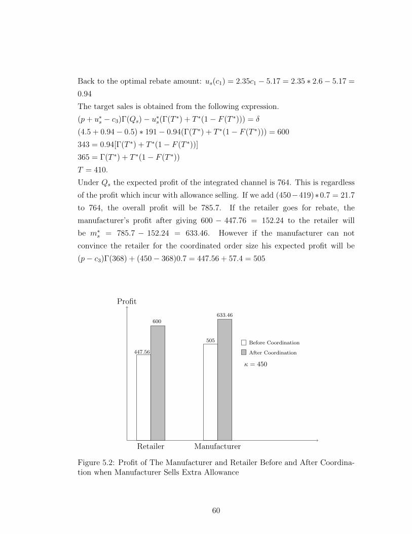
Back to the optimal rebate amount: us(c1) = 2.35c1 − 5.17 = 2.35 ∗ 2.6− 5.17 =

0.94

The target sales is obtained from the following expression.

(p+ u∗s − c3)Γ(Qs)− u∗s(Γ(T ∗) + T ∗(1− F (T ∗))) = δ

(4.5 + 0.94− 0.5) ∗ 191− 0.94(Γ(T ∗) + T ∗(1− F (T ∗))) = 600

343 = 0.94[Γ(T ∗) + T ∗(1− F (T ∗))]

365 = Γ(T ∗) + T ∗(1− F (T ∗))

T = 410.

Under Qs the expected profit of the integrated channel is 764. This is regardless

of the profit which incur with allowance selling. If we add (450−419)∗0.7 = 21.7

to 764, the overall profit will be 785.7. If the retailer goes for rebate, the

manufacturer’s profit after giving 600 − 447.76 = 152.24 to the retailer will

be m∗s = 785.7 − 152.24 = 633.46. However if the manufacturer can not

convince the retailer for the coordinated order size his expected profit will be

(p− c3)Γ(368) + (450− 368)0.7 = 447.56 + 57.4 = 505

Profit

Retailer

447.56

600

Manufacturer

505

633.46

Before Coordination

After Coordination

κ = 450

Figure 5.2: Profit of The Manufacturer and Retailer Before and After Coordina-tion when Manufacturer Sells Extra Allowance

60

Chapter 6

Extensions and Conclusion

In this chapter, we review how the findings contribute to the objective of the

thesis. We have studied the coordination of a manufacturer and a retailer under

the cap and trade regulation of carbon emission. To this end, the conditions of

optimality for the parameters of different contract types are uncovered. We have

created a conceptual model of each contract type. Return and rebate contracts

have been investigated in detail. We have demonstrated how contracting param-

eters can be derived based on the profit share in order to achieve coordination.

We have explored and analyzed supply chain coordination where the drivers of

each contract type are discussed and the optimal values are found.

Our results for the return contract show that when no returns is allowed, the

manufacturer and retailer may achieve coordination. In this case, the wholesale

price is set such that the revenue or loss due to the selling and buying the limit is

shared between the members. Besides, when the manufacturer allows for full re-

turns, the channel may be coordinated as well. We looked for such combinations

of wholesale price and the return price which increased the expected profit of both

manufacturer and retailer compared to the uncoordinated channel and a win-win

outcome. The results show that, instead of selling the extra emission allowance

to the market, the manufacturer stimulates the retailer to order channel optimal

order size rather than retailer’s optimal. This way, an increase in the manufac-

turer’s profit margin is observed which exceeds the profit from the selling of extra

61

allowance to the market directly. In the buying region the intuition is straightfor-

ward. The manufacturer benefits from selling the product to the retailer; even if

he incurs the cost of buying the required emission allowance. The profit from the

unit production is larger than the unit emission cost. Consequently, whatever the

retailer’s optimal order is, the manufacturer offers the retailer to order channel

optimal. Due to the increase in the retailer’s expected profit, he will accept the

offer. Finally in ”Do Nothing” region, the manufacturer neither buys nor sells

any allowance. Based on our numerical results, an increase to the expected profits

of both parties after the practice of coordination was incurred. However in ”Do

Nothing” region, the case of no returns was costly for the manufacturing part.

In fact, the retailer accepts the channel optimal order size with a wholesale price

which is not interesting for the manufacturer.

In short the results of the return contract is as follows:

1. Coordination is achievable even if no returns is allowed.

2. If full returns with full credit is allowed, the channel could not be coordi-

nated.

3. If full returns with partial credit is allowed, the channel could be coordi-

nated.

4. Coordination can be a profit maximizing action in all cases considered,

except in κ/β region with no returns permission.

5. If selling and buying prices are close together, the Qs and Qb will approach

together. This leads to a single ordering policy for the manufacturer.

6. The more larger the assigned cap is, the more profit will be incured for

both manufacturer and retailer. Similarly small vales of cap decreases the

corresponding profits of manufacturer and retailer.

7. If the assigned cap converges to zero, the manufacturer will accept the

retailer’s optimal instead of motivating him for channel optimal.

62

For the rebate contract the results are summarized as follows:

1. Coordination is achievable with appropriate choices of target sales, rebate

and wholesale price.

2. Manufacturer has to sacrifice a proportion of his expected revenue due to

coordination practice in order to motivate the retailer for channel optimal

order quantity.

3. As the assigned κ increases, the manufacturer will be able to offer larger

increases to retailer’s profit by reducing the wholesale price and reducing

target sales.

4. Small values of κ restricts the manufacturer to offer more profit to the

retailer in order to motivate him for the channel optimal order quantity.

Other directions for future research include the coordination issue with the supply

chain composed of a manufacturer, a distributor and a retailer. How to determine

the coordination method when the incentive factor for less emission is incorpo-

rated, can also be a future work. The competing retailers and manufacturers

case could also be an extension for this research. It would also be interesting to

extend our single-period setting into a multi-period one, with consideration of or-

dering and production policies of the retailer and the manufacturer over multiple

planning horizons.

63

Bibliography

[1] W. G. Egelhoff, “Information-processing theory and the multinational en-

terprise,” Journal of international business studies, pp. 341–368, 1991.

[2] F. Sahin and E. P. Robinson, “Flow coordination and information sharing

in supply chains: review, implications, and directions for future research,”

Decision Sciences, vol. 33, no. 4, pp. 505–536, 2002.

[3] A. A. Tsay, “The quantity flexibility contract and supplier-customer incen-

tives,” Management science, vol. 45, no. 10, pp. 1339–1358, 1999.

[4] L. Gangadharan, “Analysis of prices in tradable emission markets: an empir-

ical study of the regional clean air incentives market in los angeles,” Applied

Economics, vol. 36, no. 14, pp. 1569–1582, 2004.

[5] S. K. Srivastava, “Green supply-chain management: a state-of-the-art liter-

ature review,” International journal of management reviews, vol. 9, no. 1,

pp. 53–80, 2007.

[6] B. A. Pasternack, “Optimal pricing and return policies for perishable com-

modities,” Marketing science, vol. 27, no. 1, pp. 133–140, 2008.

[7] M. A. Lariviere and E. L. Porteus, “Selling to the newsvendor: An analysis

of price-only contracts,” Manufacturing & service operations management,

vol. 3, no. 4, pp. 293–305, 2001.

[8] D. Wu, “Coordination of competing supply chains with news-vendor and

buyback contract,” International Journal of Production Economics, vol. 144,

no. 1, pp. 1–13, 2013.

64

[9] T. Xiao, K. Shi, and D. Yang, “Coordination of a supply chain with consumer

return under demand uncertainty,” International Journal of Production Eco-

nomics, vol. 124, no. 1, pp. 171–180, 2010.

[10] T. A. Taylor, “Supply chain coordination under channel rebates with sales

effort effects,” Management science, vol. 48, no. 8, pp. 992–1007, 2002.

[11] W.-K. Wong, J. Qi, and S. Leung, “Coordinating supply chains with sales

rebate contracts and vendor-managed inventory,” International Journal of

Production Economics, vol. 120, no. 1, pp. 151–161, 2009.

[12] G. P. Cachon and M. A. Lariviere, “Supply chain coordination with revenue-

sharing contracts: strengths and limitations,” Management science, vol. 51,

no. 1, pp. 30–44, 2005.

[13] A. P. Jeuland and S. M. Shugan, “Managing channel profits,” Marketing

science, vol. 2, no. 3, pp. 239–272, 1983.

[14] J. Li and L. Liu, “Supply chain coordination with quantity discount policy,”

International Journal of Production Economics, vol. 101, no. 1, pp. 89–98,

2006.

[15] D. Ghosh and J. Shah, “A comparative analysis of greening policies across

supply chain structures,” International Journal of Production Economics,

vol. 135, no. 2, pp. 568–583, 2012.

[16] J. Song and M. Leng, “Analysis of the single-period problem under car-

bon emissions policies,” in Handbook of Newsvendor Problems, pp. 297–313,

Springer, 2012.

[17] X. Liang and Y. Xiong, “Emissions reduction cost-sharing contract through

green innovation under carbon emission constraints,” Key Engineering Ma-

terials, vol. 572, pp. 663–667, 2014.

[18] X. Liang, Y. Xiong, Y. Z. Hou, and S. M. Xia, “Pricing and emission reduc-

tion strategy of manufacturer with carbon emission constraints in low carbon

supply chain,” Key Engineering Materials, vol. 572, pp. 659–662, 2014.

65

[19] N. Ma and X. L. Gao, “Supply chain contract arrangements of carbon abate-

ment with consumer preferences,” Applied Mechanics and Materials, vol. 260,

pp. 759–764, 2013.

[20] S. Benjaafar, Y. Li, and M. Daskin, “Carbon footprint and the management

of supply chains: Insights from simple models,” Automation Science and

Engineering, IEEE Transactions on, vol. 10, no. 1, pp. 99–116, 2013.

[21] X. Chen, S. Benjaafar, and A. Elomri, “The carbon-constrained eoq,” Op-

erations Research Letters, vol. 41, no. 2, pp. 172–179, 2013.

[22] M. Y. Jaber, C. H. Glock, and A. M. El Saadany, “Supply chain coordination

with emissions reduction incentives,” International Journal of Production

Research, vol. 51, no. 1, pp. 69–82, 2013.

[23] S. Du, L. Zhu, L. Liang, and F. Ma, “Emission-dependent supply chain

and environment-policy-making in the cap-and-tradesystem,” Energy Policy,

vol. 57, pp. 61–67, 2013.

[24] G. Hua, T. Cheng, and S. Wang, “Managing carbon footprints in inven-

tory management,” International Journal of Production Economics, vol. 132,

no. 2, pp. 178–185, 2011.

[25] J.-J. Zhang, T.-F. Nie, and S.-F. Du, “Optimal emission-dependent pro-

duction policy with stochastic demand,” International Journal of Society

Systems Science, vol. 3, no. 1, pp. 21–39, 2011.

[26] S. Zanoni, L. Mazzoldi, L. E. Zavanella, and M. Y. Jaber, “A joint economic

lot size model with price and environmentally sensitive demand,” Production

& Manufacturing Research, vol. 2, no. 1, pp. 341–354, 2014.

[27] A. Toptal, H. Ozlu, and D. Konur, “Joint decisions on inventory replen-

ishment and emission reduction investment under different emission regula-

tions,” International Journal of Production Research, vol. 52, no. 1, pp. 243–

269, 2014.

66

[28] S. Swami and J. Shah, “Channel coordination in green supply chain manage-

ment,” Journal of the Operational Research Society, vol. 64, no. 3, pp. 336–

351, 2012.

[29] T. M. Whitin, “Inventory control and price theory,” Management science,

vol. 2, no. 1, pp. 61–68, 1955.

[30] H. Lau and A.-L. Lau, “A semi-analytical solution for a newsboy problem

with mid-period replenishment,” Journal of the Operational Research Soci-

ety, vol. 48, no. 12, pp. 1245–1259, 1997.

[31] M. Khouja, “The single-period (news-vendor) problem: literature review and

suggestions for future research,” Omega, vol. 27, no. 5, pp. 537–553, 1999.

[32] H. Shore, “A general solution for the newsboy model with random order size

and possibly a cutoff transaction size,” Journal of the Operational Research

Society, vol. 55, no. 11, pp. 1218–1228, 2004.

[33] S. Sozuer, “On the newsvendor problem with multiple inputs under a carbon

emission constraint,” Master’s thesis, Bilkent University, 2012.

[34] O. Korkmaz, “Carbon restricted newsvendor problem under cvar objective

and resource constraints,” Master’s thesis, Bilkent University, 2014.

67

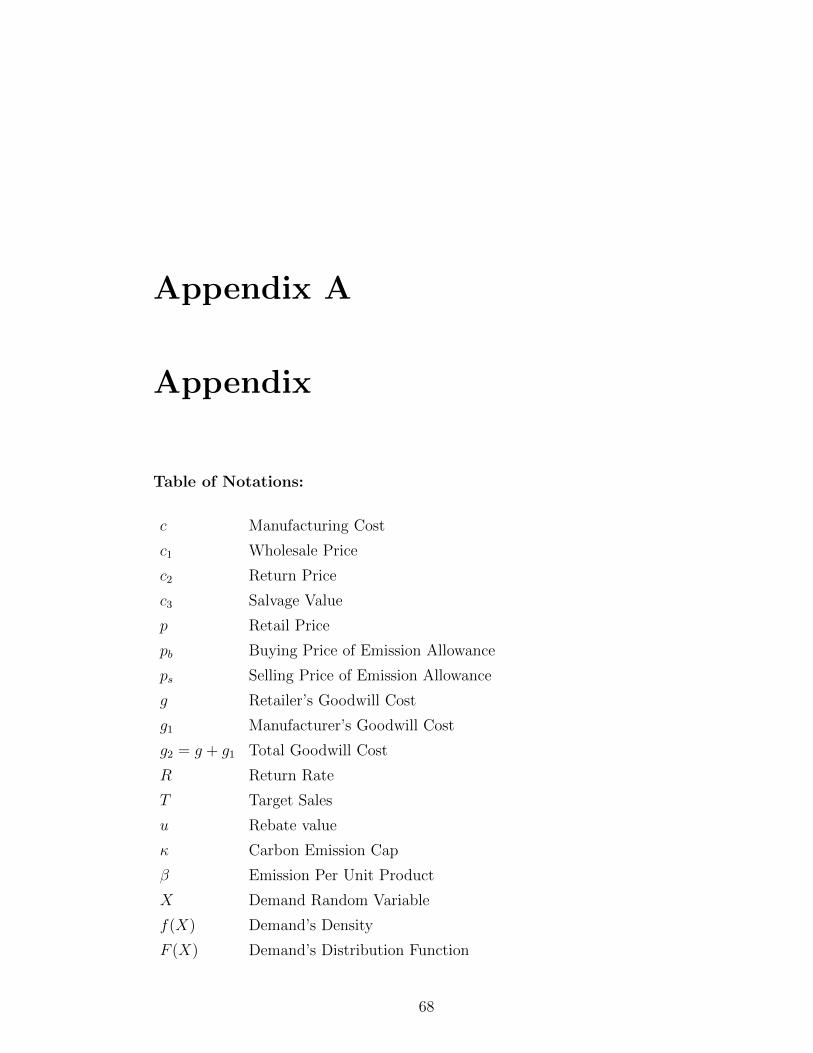
Appendix A

Appendix

Table of Notations:

c Manufacturing Cost

c1 Wholesale Price

c2 Return Price

c3 Salvage Value

p Retail Price

pb Buying Price of Emission Allowance

ps Selling Price of Emission Allowance

g Retailer’s Goodwill Cost

g1 Manufacturer’s Goodwill Cost

g2 = g + g1 Total Goodwill Cost

R Return Rate

T Target Sales

u Rebate value

κ Carbon Emission Cap

β Emission Per Unit Product

X Demand Random Variable

f(X) Demand’s Density

F (X) Demand’s Distribution Function

68