brown university, may 1999.cs.brown.edu/research/pubs/theses/phd/1999/cherniack.pdf · brown...
TRANSCRIPT

Abstract of “Building Query Optimizers with Combinators” by Mitch Cherniack, Ph.D.,
Brown University, May 1999.
Query optimizers generate plans to retrieve data requested by queries. Optimizers are hard
to build because for any given query, there can be a prohibitively large number of plans to
choose from. Typically, the complexity of optimization is handled by dividing optimization
into two phases: a heuristic phase (called query rewriting) that narrows the space of plans
to consider, and a cost-based phase that compares the relative merits of plans that lie in the
narrowed space.
The goal of query rewriting is to transform queries into equivalent queries that are
more amenable to plan generation. This process has proven to be error-prone. Rewrites
over nested queries and queries returning duplicates have been especially problematic, as
evidenced by the well-known COUNT bug of the unnesting rewrites of Kim. The advent of
object-oriented and object-relational databases only exacerbates this issue by introducing
more complex data and by implication, more complex queries and query rewrites.
This thesis addresses the correctness issue for query rewriting. We introduce a novel
framework (COKO-KOLA) for expressing query rewrites that can be verified with an au-
tomated theorem prover. At its foundation lies KOLA: our combinator-based query algebra
that permits expression of simple query rewrites (rewrite rules) without imperative code.
While rewrite rules are easily verified, they lack the expressivity to capture many query
rewrites used in practice. We address this issue in two ways:
• We introduce a language (COKO) to express complex query transformations using
KOLA rule sets and an algorithm to control rule firing. COKO supports expression
of query rewrites that are too general to be expressed with rewrite rules alone.
• We extend KOLA to permit expression of rewrite rules whose firing requires inferring
semantic conditions. This extension permits expression of query rewrites that are too
specific to be expressed with rewrite rules alone.
The recurring theme of this work is that all of the proposed techniques are made possible
by a combinator-based representation of queries.

Building Query Optimizers with Combinators
by
Mitch Cherniack
B. Ed., McGill University, Montreal, Canada, 1984
Dip. Ed., McGill University, Montreal, Canada, 1985
Dip. Comp. Sci., Concordia University, Montreal, Canada, 1990
M. Comp. Sci., Concordia University, Montreal, Canada, 1992
A dissertation submitted in partial fulfillment of the
requirements for the Degree of Doctor of Philosophy
in the Department of Computer Science at Brown University
Providence, Rhode Island
May 1999

c© Copyright 1995, 1996, 1998, 1999 by Mitch Cherniack

This dissertation by Mitch Cherniack is accepted in its present form by
the Department of Computer Science as satisfying the dissertation requirement
for the degree of Doctor of Philosophy.
DateStan Zdonik, Director
Recommended to the Graduate Council
DatePascal Van Hentenryck, Reader
DateDave Maier, Reader
Oregon Graduate Institute
DateJoe Hellerstein, Reader
University of California, Berkeley
Approved by the Graduate Council
DatePeder J. Estrup
Dean of the Graduate School and Research
ii

Vita
Mitch Cherniack was born on August 18th, 1963 in Winnipeg, Canada. He completed
secondary school in Denver, Colorado, and then attended McGill University in Montreal,
Canada, where he received his Bachelor of Education degree (Elementary) in 1984, and a
Diploma of Education degree (Secondary) in 1985. He taught in the far north of Canada for
a time in 1984, and then taught high school Computer Science and Mathematics in Montreal
from 1985–1989. He returned to school at Concordia University in Montreal in 1989, and
subsequently earned a Diploma in Computer Science in 1990, and a Masters degree in
Computer Science in 1992. He then joined the doctoral program at Brown University in
the fall of 1992.
iii

Acknowledgements
This thesis work could not have been completed without the help and support of colleagues,
friends and family. I have been lucky in my time at Brown to be surrounded by so many
talented people. I would first like to thank my fellow graduate students in Computer Science
departments here at Brown and elsewhere, with whom I drank late night coffees while
sharing thoughts about our work and our lives. Swarup Acharya was my contemporary
in the database group at Brown. Swarup was an endless source of information, support
and good humor. Among the database students who preceded me, I would especially
like to thank Ted Leung and Bharathi Subramanian for showing me the ropes, and Misty
Nodine who took me under her wing upon my arrival at Brown. Michael Littman and Tony
Cassandra, though not members of the database group, provided invaluable feedback on
ideas that I presented to them and became close friends. Outside of Brown, Bennet Vance
of Oregon Graduate Institute (and now at IBM, Almaden) has been an invaluable source
of advice on all things mathematical. My apologies, Bennet, for keeping you up so late at
SIGMOD every year. I also benefited from many fruitful discussions with Leo Fegaras (now
at the University of Texas, Arlington), Eui-Suk Chung (of Ericsson), Torsten Grust of the
University of Konstanz, and Joachim Kroger of the University of Rostock.
I would like to thank the students who worked on the implementations of this work.
Blossom Sumulong worked on the dynamic query rewriting implementation presented in
Chapter 7 as part of her Masters thesis. Kee Eung Kim and Joon Suk Lee built the initial
COKO compiler described in Chapter 4 as a class project for a graduate seminar. I am
especially grateful to Joon who maintained the compiler implementation in the face of many
requests for revisions, and who added the semantic extensions to the compiler described in
Chapter 5 as part of the work for his Masters thesis.
The administrative and technical staffs of the Computer Science at Brown went far
beyond the call of duty in answering my many requests for assistance. For this help, I
would especially like to acknowledge the help of Mary Andrade, Kathy Kirman, Max Salvas
iv
and Jeff Coady.
Working at Brown gave me the opportunity to meet many members of the database
and formal methods research communities. I owe my initial interest in formal methods to
discussions held with John Guttag of MIT. Steve Garland of MIT was an endless provider
of knowledge and advice on using Larch. While designing KOLA, we had many useful
discussions with Barbara Liskov and her programming methodology group at MIT. Catriel
Beeri of Hebrew University was most generous with his time providing suggestions and
criticisms, as was Tamer Oszu of the University of Alberta who also provided personal and
professional guidance to me during his visits here and my visit to Alberta. Ashok Malhotra
of the T.J. Watson Research Division of IBM was an early supporter of this work, and
was instrumental in our successful efforts to receive a Partnership Grant from IBM. The
database reading group of the Oregon Graduate Institute provided much useful feedback
during the early development of KOLA, as did Gail Mitchell of GTE who doubly served as
a reader for each of our conference submissions.
Each of the members of my thesis committee provided extremely valuable advice long
before we asked them to serve on my committee. Joe Hellerstein, whom I met when he
visited here, pushed us to explore the Starburst query rewrites (especially the Magic Sets
rewrites) as an expressivity challenge for COKO. I am indebted to Joe for our many lengthy
discussions held at the various SIGMOD and VLDB conferences where we met. Dave Maier
also provided early advice and was the one who encouraged study of work done by the
functional programming community on combinators. Finally, Pascal Van Hentenryck proved
to be a tremendous resource for the functional programming and programming language
design components of this work, and also proved to be especially helpful during my job
search.
I would like to thank all of my friends who were so supportive of me during some of the
personally difficult years during my time here. My friends in Montreal provided an oasis to
escape to when times were especially difficult. I would like to thank Leslie Silverstein and
Helene Brunet, Nicole Allard and Paul Duarte, Peggy Hoffman, Peter Grogono and Sharon
Nelson, Elizabeth Wiener, Diane Bouwman, Jeff Karp and Daniel Nonen for their support
and friendship. I’d also like to thank my close friends here in New England: Sonia Leach,
Kathy Kirman, Grace Ashton, Adrienne Suvajian, Rob Netzer and Carol Collins, and Gail
Mitchell and Stan Zdonik.
My family has been a wonderful source of support, love and strength. My sister Karen
has been a source of encouragement from the onset, providing me with computer equipment
when I couldn’t afford my own and providing sisterly advice along the way. My brother
v

Mark is my closest friend, and has always been there for me whenever I have needed him
to be. And my parents, Edith and Reuben Cherniack have helped me out in every possible
way. In my last few months at Brown when circumstances forced me to leave Rhode Island,
they welcomed me back home and reminded me through their generosity and kindness of
all that they have done for me throughout my life. Mom and Dad, this thesis would not
have happened if not for you.
Finally, I would like to thank my two mentors who are primarily responsible for my
development as a researcher. Peter Grogono, my Masters degree supervisor at Concordia
University, is quite simply the best teacher I have ever known. I aspire to teach and write
as well as he does, and I know that I have a lifelong challenge ahead of me in trying to
meet this goal. I also owe Peter thanks for exposing me to the excitement of research and
to the elegance of mathematics; neither of which I knew before enrolling at Concordia over
10 years ago.
Lastly, I cannot possibly express the depth of gratitude I feel for my Ph.D. supervisor,
Stan Zdonik. Stan has been an ideal supervisor. He helped me to see the big picture in
research when I got lost in details. He taught me how to communicate my ideas effectively,
both in writing and in presentation. He gave me confidence by being a constant source of
moral support, and by maintaining excitement about my work. Perhaps most importantly
to me, Stan has been a close friend. He and Gail took me into their home when I had
nowhere else to go — for this and so much more, I will always be grateful.
vi

Credits
Some of these chapters are adapted from our papers. Chapter 3 is based on our 1996
SIGMOD paper [22] and our 1995 DBPL paper [23]. Chapter 4 is based on our 1998
SIGMOD paper [20]. Chapter 5 is based on our 1998 VLDB paper [21]. Chapter 6 is based
on a recent conference submission [19]. Chapter 7 forms the basis of a paper currently in
preparation. All of these papers were written jointly with Stan Zdonik. As well, [23] was
written jointly with Marian H. Nodine and [19] was written jointly with Ashok Malhotra.
Joon Suk Lee and Kee-Eung Kim were primarily responsible for the implementation
of the compiler described in Chapter 4. Joon Suk Lee implemented the semantic exten-
sions described in Chapter 5. Blossom Sumulong is building the prototype implementation
described in Chapter 7.
I was supported by numerous grants during my time at Brown, including ONR grant
number N00014-91-J-4052 under ARPA order number 8225 and contract DAAB-07-91-C-
Q518 under subcontract F41100, NSF grant IRI 9632629, and a gift from the IBM corpo-
ration. I gratefully acknowledge this support.
vii

Contents
List of Tables xiii
List of Figures xiv
1 Introduction 1
1.1 Preliminaries . . . . . . . . . . . . . . . . . . . . . . . . . . . . . . . . . . . 1
1.1.1 Query Optimization . . . . . . . . . . . . . . . . . . . . . . . . . . . 3
1.1.2 Query Rewriting . . . . . . . . . . . . . . . . . . . . . . . . . . . . . 3
1.1.3 Rule-Based Query Optimizers and Query Rewriters . . . . . . . . . 4
1.2 Issues in Query Rewriting . . . . . . . . . . . . . . . . . . . . . . . . . . . . 5
1.2.1 The Correctness Issue . . . . . . . . . . . . . . . . . . . . . . . . . . 5
1.2.2 The Expressivity Issue . . . . . . . . . . . . . . . . . . . . . . . . . . 6
1.3 Contributions . . . . . . . . . . . . . . . . . . . . . . . . . . . . . . . . . . . 6
1.3.1 Conceptual Contributions . . . . . . . . . . . . . . . . . . . . . . . . 6
1.3.2 Implementations . . . . . . . . . . . . . . . . . . . . . . . . . . . . . 7
1.3.3 High-Level Contributions . . . . . . . . . . . . . . . . . . . . . . . . 7
1.4 Outline . . . . . . . . . . . . . . . . . . . . . . . . . . . . . . . . . . . . . . 8
2 Motivation 10
2.1 The Thomas Website . . . . . . . . . . . . . . . . . . . . . . . . . . . . . . . 10
2.2 An Object Database Schema for Thomas . . . . . . . . . . . . . . . . . . . 11
2.3 The “Conflict of Interests” Queries (COI) . . . . . . . . . . . . . . . . . . . 13
2.3.1 Naive Evaluation of COI1 . . . . . . . . . . . . . . . . . . . . . . . . 14
2.3.2 A Complex Query Rewrite for COI1 . . . . . . . . . . . . . . . . . . 15
2.3.3 Correctness . . . . . . . . . . . . . . . . . . . . . . . . . . . . . . . . 16
2.4 The “NSF” Queries (NSF) . . . . . . . . . . . . . . . . . . . . . . . . . . . 17
2.4.1 Naive Evaluation of NSF1 . . . . . . . . . . . . . . . . . . . . . . . . 18
viii

2.4.2 A Semantic Query Rewrite for NSF1 . . . . . . . . . . . . . . . . . . 18
2.4.3 Dynamic Query Rewriting . . . . . . . . . . . . . . . . . . . . . . . . 20
2.5 Chapter Summary . . . . . . . . . . . . . . . . . . . . . . . . . . . . . . . . 21
3 KOLA: Correct Query Rewrites 22
3.1 The Need for a Combinator-Based Query Algebra . . . . . . . . . . . . . . . 22
3.1.1 Variables Considered Harmful . . . . . . . . . . . . . . . . . . . . . 23
3.1.2 The Need for a Combinator-Based Query Algebra: Summary . . . . 29
3.2 KOLA . . . . . . . . . . . . . . . . . . . . . . . . . . . . . . . . . . . . . . 30
3.2.1 An OQL Query Expressed in KOLA . . . . . . . . . . . . . . . . . . 30
3.2.2 The KOLA Data Model . . . . . . . . . . . . . . . . . . . . . . . . . 33
3.2.3 KOLA Primitives and Formers . . . . . . . . . . . . . . . . . . . . . 37
3.3 Using a Theorem Prover to Verify KOLA Rewrites . . . . . . . . . . . . . . 44
3.3.1 A Formal Specification of KOLA Using LSL . . . . . . . . . . . . . . 44
3.3.2 Proving KOLA Rewrite Rules Using LP . . . . . . . . . . . . . . . . 46
3.4 Revisiting the “Conflict of Interests” Queries . . . . . . . . . . . . . . . . . 50
3.4.1 KOLA Translations of the COI Queries . . . . . . . . . . . . . . . . 50
3.4.2 A Rule Set for Rewriting the COI Queries . . . . . . . . . . . . . . 62
3.5 Discussion . . . . . . . . . . . . . . . . . . . . . . . . . . . . . . . . . . . . . 66
3.5.1 The Expressive Power of KOLA . . . . . . . . . . . . . . . . . . . . 66
3.5.2 Addressing the Downsides of KOLA . . . . . . . . . . . . . . . . . . 67
3.6 Chapter Summary . . . . . . . . . . . . . . . . . . . . . . . . . . . . . . . . 68
4 COKO: Complex Query Rewrites 70
4.1 Why COKO? . . . . . . . . . . . . . . . . . . . . . . . . . . . . . . . . . . . 71
4.2 Example 1: CNF . . . . . . . . . . . . . . . . . . . . . . . . . . . . . . . . . 72
4.2.1 CNF for KOLA Predicates . . . . . . . . . . . . . . . . . . . . . . . 72
4.2.2 An Exhaustive Firing Algorithm . . . . . . . . . . . . . . . . . . . . 73
4.2.3 A Non-Exhaustive Firing Algorithm for CNF . . . . . . . . . . . . . 77
4.3 The Language of COKO Firing Algorithms . . . . . . . . . . . . . . . . . . 83
4.3.1 The COKO Language . . . . . . . . . . . . . . . . . . . . . . . . . . 84
4.3.2 TRUE, FALSE and SKIP . . . . . . . . . . . . . . . . . . . . . . . . . . 87
4.3.3 The COKO Compiler . . . . . . . . . . . . . . . . . . . . . . . . . . 87
4.4 Example 2: “Separated Normal Form” (SNF) . . . . . . . . . . . . . . . . 88
4.4.1 Definitions . . . . . . . . . . . . . . . . . . . . . . . . . . . . . . . . 89
ix

4.4.2 A COKO Transformation for SNF . . . . . . . . . . . . . . . . . . . 91
4.5 Example Applications of SNF . . . . . . . . . . . . . . . . . . . . . . . . . . 107
4.5.1 Example 3: Predicate-Pushdown . . . . . . . . . . . . . . . . . . . . 107
4.5.2 Example 4: Join-Reordering . . . . . . . . . . . . . . . . . . . . . . 107
4.6 Example 5: Magic-Sets . . . . . . . . . . . . . . . . . . . . . . . . . . . . . 109
4.6.1 An Example Magic-Sets Rewrite . . . . . . . . . . . . . . . . . . . . 110
4.6.2 Expressing Magic-Sets in COKO . . . . . . . . . . . . . . . . . . . . 114
4.7 Discussion . . . . . . . . . . . . . . . . . . . . . . . . . . . . . . . . . . . . 121
4.7.1 The Expressivity of COKO . . . . . . . . . . . . . . . . . . . . . . . 121
4.7.2 The Need for Normalization . . . . . . . . . . . . . . . . . . . . . . . 122
4.8 Chapter Summary . . . . . . . . . . . . . . . . . . . . . . . . . . . . . . . . 123
5 Semantic Query Rewrites 125
5.1 Example 1: Injectivity . . . . . . . . . . . . . . . . . . . . . . . . . . . . . . 127
5.1.1 Expressing Semantic Query Rewrites in COKO-KOLA . . . . . . . . 130
5.1.2 Correctness . . . . . . . . . . . . . . . . . . . . . . . . . . . . . . . . 133
5.1.3 Revisiting the “NSF” Query of Chapter 2 . . . . . . . . . . . . . . . 134
5.1.4 More Uses for Injectivity . . . . . . . . . . . . . . . . . . . . . . . . 135
5.2 Example 2: Predicate Strength . . . . . . . . . . . . . . . . . . . . . . . . . 136
5.2.1 Some Rewrite Rules Conditioned on Predicate Strength . . . . . . . 136
5.2.2 A COKO Property for Predicate Strength . . . . . . . . . . . . . . . 137
5.2.3 Example Uses of Predicate Strength . . . . . . . . . . . . . . . . . . 138
5.3 Implementation . . . . . . . . . . . . . . . . . . . . . . . . . . . . . . . . . 141
5.3.1 Implementation Overview . . . . . . . . . . . . . . . . . . . . . . . . 141
5.3.2 Performing Inference . . . . . . . . . . . . . . . . . . . . . . . . . . 142
5.3.3 Integrating Inference and Rule Firing . . . . . . . . . . . . . . . . . 144
5.4 Discussion . . . . . . . . . . . . . . . . . . . . . . . . . . . . . . . . . . . . 145
5.4.1 Benefits to this Approach . . . . . . . . . . . . . . . . . . . . . . . . 145
5.4.2 The Advantage of KOLA . . . . . . . . . . . . . . . . . . . . . . . . 147
5.5 Chapter Summary . . . . . . . . . . . . . . . . . . . . . . . . . . . . . . . . 148
6 Experiences With COKO-KOLA 149
6.1 Background . . . . . . . . . . . . . . . . . . . . . . . . . . . . . . . . . . . 150
6.1.1 San Francisco Object Model . . . . . . . . . . . . . . . . . . . . . . . 150
6.1.2 Relational Implementation of the Object Model . . . . . . . . . . . . 151
x

6.1.3 Querying . . . . . . . . . . . . . . . . . . . . . . . . . . . . . . . . . 152
6.1.4 Our Contribution . . . . . . . . . . . . . . . . . . . . . . . . . . . . . 153
6.2 Translating Query Lite Queries into KOLA . . . . . . . . . . . . . . . . . . 153
6.2.1 Translation Strategies . . . . . . . . . . . . . . . . . . . . . . . . . . 156
6.2.2 T: The Query Lite → KOLA Translation Function Described . . . . 160
6.2.3 Sample Traces of Translation . . . . . . . . . . . . . . . . . . . . . . 167
6.2.4 Translator Implementation . . . . . . . . . . . . . . . . . . . . . . . 171
6.3 Query Rewriting . . . . . . . . . . . . . . . . . . . . . . . . . . . . . . . . . 172
6.3.1 A Library of General-Purpose COKO Transformations . . . . . . . 172
6.3.2 Normalizing the Results of Translation . . . . . . . . . . . . . . . . 183
6.3.3 Transforming Path Expressions to Joins . . . . . . . . . . . . . . . . 200
6.4 Translating KOLA into SQL . . . . . . . . . . . . . . . . . . . . . . . . . . 210
6.5 Discussion . . . . . . . . . . . . . . . . . . . . . . . . . . . . . . . . . . . . 214
6.5.1 Integration Capabilities of COKO-KOLA . . . . . . . . . . . . . . . 214
6.5.2 Ease-Of-Use of COKO-KOLA . . . . . . . . . . . . . . . . . . . . . . 217
6.6 Chapter Summary . . . . . . . . . . . . . . . . . . . . . . . . . . . . . . . . 221
7 Dynamic Query Rewriting 223
7.1 A Dynamic Query Rewriter for ObjectStore . . . . . . . . . . . . . . . . . 224
7.1.1 Making ObjectStore Objects Queryable . . . . . . . . . . . . . . . . 225
7.1.2 Iterators . . . . . . . . . . . . . . . . . . . . . . . . . . . . . . . . . 227
7.1.3 Combining Rewriting With Evaluation . . . . . . . . . . . . . . . . . 229
7.2 Putting It All Together: The NSF Query . . . . . . . . . . . . . . . . . . . 236
7.2.1 Initial Rewriting and Evaluation . . . . . . . . . . . . . . . . . . . . 236
7.2.2 Dynamic Query Rewriting: Extracting Elements from the Result . . 236
7.2.3 Extracting Results from the Nested Query . . . . . . . . . . . . . . . 242
7.3 Discussion . . . . . . . . . . . . . . . . . . . . . . . . . . . . . . . . . . . . 248
7.3.1 Cost Considerations . . . . . . . . . . . . . . . . . . . . . . . . . . . 248
7.3.2 The Advantage of KOLA . . . . . . . . . . . . . . . . . . . . . . . . 250
7.4 Chapter Summary . . . . . . . . . . . . . . . . . . . . . . . . . . . . . . . . 250
8 Related Work 252
8.1 KOLA . . . . . . . . . . . . . . . . . . . . . . . . . . . . . . . . . . . . . . . 252
8.1.1 KOLA and Query Algebras . . . . . . . . . . . . . . . . . . . . . . . 253
8.1.2 KOLA and Combinators . . . . . . . . . . . . . . . . . . . . . . . . . 256
xi

8.1.3 KOLA and Query Calculii . . . . . . . . . . . . . . . . . . . . . . . . 258
8.2 COKO . . . . . . . . . . . . . . . . . . . . . . . . . . . . . . . . . . . . . . . 259
8.2.1 Systems that Express Complex Query Rewrites With Single Rules . 259
8.2.2 Systems that Express Complex Query Rewrites With Rule Groups . 261
8.2.3 Theorem Provers . . . . . . . . . . . . . . . . . . . . . . . . . . . . . 262
8.3 Semantic Query Rewriting . . . . . . . . . . . . . . . . . . . . . . . . . . . . 263
8.3.1 Semantic Optimization Strategies . . . . . . . . . . . . . . . . . . . . 263
8.3.2 Semantic Optimization Frameworks . . . . . . . . . . . . . . . . . . 264
8.4 Dynamic Query Rewriting . . . . . . . . . . . . . . . . . . . . . . . . . . . . 268
8.4.1 Dynamic Plan Selection . . . . . . . . . . . . . . . . . . . . . . . . . 269
8.4.2 Adaptive Query Optimization . . . . . . . . . . . . . . . . . . . . . 271
8.4.3 Partial Evaluation . . . . . . . . . . . . . . . . . . . . . . . . . . . . 272
9 Conclusions and Future Work 274
9.1 Future Directions . . . . . . . . . . . . . . . . . . . . . . . . . . . . . . . . . 277
9.2 Conclusions . . . . . . . . . . . . . . . . . . . . . . . . . . . . . . . . . . . . 280
A A Larch Specification of KOLA 281
A.1 Functions and Predicates . . . . . . . . . . . . . . . . . . . . . . . . . . . . 281
A.2 Objects . . . . . . . . . . . . . . . . . . . . . . . . . . . . . . . . . . . . . . 282
A.3 Primitives (Table 3.1) . . . . . . . . . . . . . . . . . . . . . . . . . . . . . . 287
A.4 Basic Formers (Table 3.2) . . . . . . . . . . . . . . . . . . . . . . . . . . . . 303
A.5 Query Formers (Table 3.3) . . . . . . . . . . . . . . . . . . . . . . . . . . . . 314
B LP Proof Scripts 329
B.1 Proof Scripts for CNF . . . . . . . . . . . . . . . . . . . . . . . . . . . . . . 329
B.2 Proof Scripts for SNF . . . . . . . . . . . . . . . . . . . . . . . . . . . . . . 329
B.3 Proof Scripts for Predicate Pushdown . . . . . . . . . . . . . . . . . . . . . 329
B.4 Proof Scripts for Magic Sets . . . . . . . . . . . . . . . . . . . . . . . . . . 329
B.5 Proof Scripts for Rules of Chapter 5 . . . . . . . . . . . . . . . . . . . . . . 329
B.6 Proof Scripts for Rules of Chapter 6 . . . . . . . . . . . . . . . . . . . . . . 329
Bibliography 330
xii

List of Tables
2.1 A Database Schema for Thomas . . . . . . . . . . . . . . . . . . . . . . . . 12
3.1 KOLA Primitives . . . . . . . . . . . . . . . . . . . . . . . . . . . . . . . . 39
3.2 Basic KOLA Formers . . . . . . . . . . . . . . . . . . . . . . . . . . . . . . 40
3.3 KOLA Query Formers . . . . . . . . . . . . . . . . . . . . . . . . . . . . . . 41
4.1 Average Times (in seconds) for CNF-TD and CNF-BU . . . . . . . . . . . . . 77
4.2 Average Times (in seconds) for CNF-TD and CNF . . . . . . . . . . . . . . . 79
4.3 Rewrite Rules Used In SimplifyJoin . . . . . . . . . . . . . . . . . . . . . 120
6.1 The Syntax of Query Lite . . . . . . . . . . . . . . . . . . . . . . . . . . . . 155
6.2 T: The Query Lite → KOLA Translation Function . . . . . . . . . . . . . . 161
6.3 Analysis of the General-Purpose COKO Transformations . . . . . . . . . . 183
6.4 Analysis of the COKO Normalization Transformations . . . . . . . . . . . 195
6.5 Analysis of the Query Lite → SQL Transformations . . . . . . . . . . . . . 210
6.6 T−1: Applied to KOLA Primitives . . . . . . . . . . . . . . . . . . . . . . . 211
6.7 T−1: Applied to KOLA Formers . . . . . . . . . . . . . . . . . . . . . . . . 215
7.1 Mappings of KOLA Operators to their Parse Tree Representations . . . . . 231
7.2 Results of Partially Evaluating and Rewriting KOLA Queries . . . . . . . . 234
7.3 Results of Evaluating KOLA Queries . . . . . . . . . . . . . . . . . . . . . 235
xiii

List of Figures
1.1 A Traditional Architecture for Query Processors . . . . . . . . . . . . . . . 2
2.1 COI1: Find all committees whose chairs belong to a subcommittee chaired by
someone from the same party. . . . . . . . . . . . . . . . . . . . . . . . . . 14
2.2 Rewriting COI1 → COI1 . . . . . . . . . . . . . . . . . . . . . . . . . . . . 15
2.3 An Incorrect Query Rewrite . . . . . . . . . . . . . . . . . . . . . . . . . . 16
2.4 NSF1: Find all House resolutions relating to the NSF and associate them with
the set of cities that are largest in districts that the bills’ sponsors represent 17
2.5 Rewriting NSF1 → NSF1 . . . . . . . . . . . . . . . . . . . . . . . . . . . . 19
2.6 NSF2: Find all Bills (Senate and House resolutions) relating to the NSF and
associate them with the set of cities that are largest in regions that the bills’
sponsors represent . . . . . . . . . . . . . . . . . . . . . . . . . . . . . . . . 20
3.1 COI2: Find all committees whose chairs belong to a party that includes some-
one that both chairs and is a member of the same subcommittee. . . . . . . 24
3.2 Transforming COI2 → COI2 → COI2 . . . . . . . . . . . . . . . . . . . . . 26
3.3 A Rewrite Rule Justifying COI2 → COI2 . . . . . . . . . . . . . . . . . . . 27
3.4 COI1∗ → COI1 (a) and a Rule to Justify It (b) . . . . . . . . . . . . . . . 28
3.5 A Simple OQL Query (a) and its KOLA Equivalent (b): Name All Subcom-
mittees Chaired by Republicans . . . . . . . . . . . . . . . . . . . . . . . . . 31
3.6 An Example LP Proof Script . . . . . . . . . . . . . . . . . . . . . . . . . . 47
3.7 Some LP Rewrite Rules Generated from Specification Axioms . . . . . . . 48
3.8 KOLA Translations of the Conflict of Interests Queries . . . . . . . . . . . 51
3.9 Rewrite Rules For the Query Rewrites of the “Conflict of Interests” Queries 63
3.10 Transforming COIK2 → COIK
2 → COIK2 . . . . . . . . . . . . . . . . . . . 64
4.1 A KOLA Predicate Before (a) and After (b) its Transformable into CNF . 74
4.2 Exhaustive CNF Transformations Expressed in COKO . . . . . . . . . . . 74
xiv

4.3 Illustrating CNF-BU on the KOLA Predicate of Figure 4.1a . . . . . . . . . 75
4.4 An Efficient CNF Transformation . . . . . . . . . . . . . . . . . . . . . . . 78
4.5 Illustrating the CNF Firing Algorithm on the KOLA Predicate of Figure 4.1a 79
4.6 The Full CNF Transformation Expressed in COKO . . . . . . . . . . . . . 82
4.7 The Effects of a GIVEN Statement on Environments . . . . . . . . . . . . . 86
4.8 The SQL/KOLA Predicates of Figure 4.1 in SNF . . . . . . . . . . . . . . 91
4.9 The SNF Normalization Expressed in COKO . . . . . . . . . . . . . . . . . 92
4.10 Auxiliary Transformations Used by SNF . . . . . . . . . . . . . . . . . . . . 93
4.11 Tracing the effects of SNF on the Predicate p of Fig 4.1a (Part 1) . . . . . . 96
4.12 Tracing the effects of SNF on the Predicate p of Fig 4.1a (Part 2) . . . . . . 97
4.13 Pushdown: A COKO Transformation to Push Predicates Past Joins . . . . 108
4.14 Join-Associate: A COKO Transformation to Reassociate a Join . . . . . 109
4.15 OQL (a) and KOLA (b) queries to find all committees whose chair is a Demo-
crat and has served more than the average number of terms of the members
of his/her chaired committees. . . . . . . . . . . . . . . . . . . . . . . . . . 110
4.16 The queries of Figure 4.15 after rewriting by Magic-Sets . . . . . . . . . . . 111
4.17 The Magic-Sets Rewrite Expressed in COKO . . . . . . . . . . . . . . . . . 114
4.18 Transformation SimpLits2 and its Auxiliary Transformation Pr2Times . . 117
5.1 The “Major Cities” (a) and “Mayors” (b) Queries Before and After Rewriting 128
5.2 KOLA Translations of Figures 5.1a and 5.1b . . . . . . . . . . . . . . . . . 129
5.3 Conditional Rewrite Rules to Eliminate Redundant Duplicate Elimination 131
5.4 Properties Defining Inference Rules for Injective Functions (a) and Sets (b) 133
5.5 NSF1k: The “NSF” Query of Figure 2.4 expressed in KOLA . . . . . . . . 134
5.6 Rewrite Rules Conditioned on Predicate Strength . . . . . . . . . . . . . . 137
5.7 A COKO Property for Predicate Strength . . . . . . . . . . . . . . . . . . 137
5.8 A Conditional Rewrite Rule Firer . . . . . . . . . . . . . . . . . . . . . . . 141
6.1 An Architecture for the Query Lite Query Rewriter . . . . . . . . . . . . . 154
6.2 OQL Queries that make Translation into KOLA Difficult . . . . . . . . . . 157
6.3 A Query Lite Query (a), its Translation (b) and its Normalization (c) . . . 158
6.4 A Prototypical OQL Query . . . . . . . . . . . . . . . . . . . . . . . . . . . 163
6.5 The Query of Figure 6.2b After deBruijn Conversion . . . . . . . . . . . . . 164
6.6 Results of Translating the OQL queries of Figure 6.2 . . . . . . . . . . . . 168
6.7 Transformation LBComp . . . . . . . . . . . . . . . . . . . . . . . . . . . . . 173
xv

6.8 Transformations LBJoin and LBJAux . . . . . . . . . . . . . . . . . . . . . . 175
6.9 Transformations LBJAyx2 and PullFP Auxiliary Transformations . . . . . . 176
6.10 Transformation SimpFunc and Its Auxiliary Transformations . . . . . . . . 177
6.11 Transformation SimpPred and Its Auxiliary Transformations . . . . . . . . 179
6.12 An Input KOLA Parse Tree to PCFAux . . . . . . . . . . . . . . . . . . . . 180
6.13 Transformation PullComFunc and Its Auxiliary Transformation . . . . . . . 182
6.14 The KOLA Query of Figure 6.6a After Normalization . . . . . . . . . . . . 184
6.15 Transformation NormTrans . . . . . . . . . . . . . . . . . . . . . . . . . . . 185
6.16 Transformation OrdUnnests . . . . . . . . . . . . . . . . . . . . . . . . . . 186
6.17 An OQL Join Query (a) and Its Translation into KOLA (b) . . . . . . . . 187
6.18 Rewrite Rules in PullP2SHRF . . . . . . . . . . . . . . . . . . . . . . . . . . 190
6.19 Translated OQL Queries Following Rewriting of their Data Functions . . . 191
6.20 Rewrite Rules in FactorK and FKAux . . . . . . . . . . . . . . . . . . . . . 192
6.21 Query 1 (a), Normalization (b), Rewrite by PEWhere (c) In SQL (d) . . . . 196
6.22 Query 2 (a), Normalization (b), Rewrite by PEWhere (c) In SQL (d) . . . . 197
6.23 Query 3 (a), Normalization (b), . . . . . . . . . . . . . . . . . . . . . . . . . 198
6.24 Query 3 (cont.) . . ., Rewrite by PEWhere (c) In SQL (d) . . . . . . . . . . . 199
6.25 Transformation PEWhere and its Auxiliary Transformation . . . . . . . . . 204
6.26 Scope Facts Assumed Known for these Examples . . . . . . . . . . . . . . 206
6.27 Property Scope and Sample Metadata Infomation Regarding Scope . . . . 207
7.1 An Alternative Architecture for Object Database Query Processors . . . . 225
7.2 The ObjectStore Queryable Class Hierarchy . . . . . . . . . . . . . . . . . . 226
7.3 The KOLA Representation Class Hierarchy . . . . . . . . . . . . . . . . . . 230
7.4 NSF2k: The KOLA Translation of Query NSF2 of Figure 2.6 . . . . . . . . 236
7.5 The Parse Tree Representation of NSF2k . . . . . . . . . . . . . . . . . . . 243
7.6 The result of calling obj and res on the “NSF Query” . . . . . . . . . . . . 244
7.7 Calling query NSF2k’s predicate on a bill, b . . . . . . . . . . . . . . . . . . 245
7.8 Calling NSF2f ’s data function on a House resolution, b . . . . . . . . . . . 246
7.9 Calling NSF2k’s inner query function on a House Representative, l . . . . . 247
xvi

Chapter 1
Introduction
Query optimizers produce plans to retrieve data specified by queries. Optimizers are inher-
ently difficult to build because for any given query, there can be a prohibitively large space
of candidate evaluation plans to consider. Further, the difficulty of formulating estimates
of plan costs makes the comparisons of plans within this space difficult. As a result, op-
timizers invariably forego searches for “best plans” and instead are considered effective if
they usually produce good plans and rarely produce poor ones.
Query optimizers are perhaps the most complex and error-prone components of databases.
In describing software testing methodology developed at Microsoft, Bill Gates reported that
hundreds of randomly generated queries were processed incorrectly by Microsoft’s SQL
Server [41]. The problem is not unique to Microsoft. Even research literature for query
optimization has been susceptible to bugs, as in the notorious “COUNT bug” revealed of
the optimization strategies proposed by Kim [63].
Software engineering has introduced formal methods for the development of correct
software. This thesis applies software engineering methodology to the development of one
error-prone component of query optimizers: the query rewriter [79].
1.1 Preliminaries
We begin by defining terms that appear throughout this thesis: query optimization, query
rewriting and rule-based query optimization and query rewriting.
1

2
Query
Query Representation
Query Representation
Query Plan
Data
Translator
Query Rewriter
Plan Generator
Query Evaluator
Figure 1.1: A Traditional Architecture for Query Processors

3
1.1.1 Query Optimization
Query optimizers typically follow an “assembly line” approach to processing queries, as
illustrated in Figure 1.1:
1. Translation first maps a query posed in a standard query language such as SQL (for
relational databases) or OQL [14] (for object-oriented databases), into an internal
representation (or algebra) manipulated by the optimizer. Example internal represen-
tations include the Query Graph Model (or QGM) which is used in Starburst [79] and
DB2, and Excess which is used in Exodus [13].
2. Query Rewriting uses heuristics to rewrite queries (more accurately, query represen-
tations) into equivalent queries that are more amenable to plan generation.1
3. Plan Generation generates alternative execution plans that retrieve the data specified
by the represented query, estimates the execution costs of each and then chooses the
one it considers “best”.
4. Plan Evaluation can immediately follow plan generation (in the case of ad hoc queries)
or can occur later if queries are compiled (as with embedded queries).
This architecture is by no means fixed. For example, Cascades [42] generates multiple
queries during query rewriting, and generates plans for each before choosing one that is
best.
1.1.2 Query Rewriting
Query rewriting has its roots in early relational databases such as System R [85] and Ingres
[92] which supported view merging: the rewriting of a query over a view into a query over the
data underlying the view. Kim [63] proposed query unnesting strategies that rewrite nested
queries (queries containing other queries) into join queries, thereby giving plan generators
more alternatives to consider. (Kim’s ideas were later refined by many, including Ganski
and Wong [39], Dayal [29] and Muralikrishnan [75, 76].) What is common to these early
proposals is that they were intended as ad hoc extensions of query optimizers.
Starburst [79] elevates these ad hoc extensions to a distinct phase of query optimization
known as query rewriting. Rewrites applied during this phase include view merging and
query unnesting, as well as other rewrites that accomplish one of the following objectives:1Some (e.g., [95]) call the heuristic preprocessing optimization stage algebraic optimization, because this
stage involves manipulation of expressions of a query algebra. The term query rewriting was introduced byStarburst [79].
4
• Normalization: Queries sometimes get posed in ways that force optimizers to choose
poor evaluation plans. For example, because query optimizers build plans incremen-
tally (i.e., by composing plans for subqueries to build full execution plans), nested
queries tend to get evaluated using nested loop algorithms. By rewriting nested
queries to join queries, optimizers are able to consider alternative algorithms such
as sort-merge joins, hash joins etc. Therefore, one goal of query rewriting is to nor-
malize a query into a form that allows a query optimizer to consider a greater number
of alternative plans.
• Improvement: Query rewriting might also apply heuristics that are likely to lead to
better plans, regardless of the contents or physical representation of the collections
being queried. An example of this is a rewrite of a query that performs duplicate
elimination into a query that does not. This rewrite is valid when duplicate elimination
is performed on a collection that is already free of duplicates (for example, a collection
resulting from projecting on a key attribute of a relation). Duplicate elimination is
costly, requiring an initial sort or grouping of the elements of a collection. Therefore,
rewriting a query to avoid duplicate elimination is always worthwhile.
1.1.3 Rule-Based Query Optimizers and Query Rewriters
With the emergence of alternative data models in the 1980’s (e.g., object-oriented) came
the need for extensible query optimizers that could adjust to variations in data. Optimizers
are extensible if they can be easily modified to account for new data models or data retrieval
techniques. Rule-based optimizers (proposed concurrently by Freytag [38] and Graefe and
DeWitt [13]) were the first optimizers introduced for this purpose.
Rule-based optimizers express the mapping of queries to plans (or queries to queries
in the case of rule-based query rewriters) incrementally in terms of rules. Rules might be
executed (fired) directly (as in Starburst, where rules are programmed in C), or used to
generate an optimizer, as with Exodus/Volcano [13, 43] which express rules as rewrite rules
supplemented with code. Rules make optimizers extensible because the behavior of the
optimizer can be modified simply by modifying its rule set. Example rule-based systems
aside from Starburst and Exodus/Volcano include Gral [6], Cascades [42] and Croque [50].
For query rewriters, rules offer a second potential benefit as formal specifications of query
rewriting behavior, making it possible for query rewriters to be formally verified. This thesis
shows how query rewrite rules can be expressed to enable their formal verification.

5
1.2 Issues in Query Rewriting
1.2.1 The Correctness Issue
As with other aspects of query optimization, query rewriting is complex and error-prone.
Definition 1.2.1 (Correctness) A query rewriter is correct if rewriting always produces
an semantically equivalent query (i.e., a query that is guaranteed to produce the same result
over all database states as the original query).
Many of Kim’s nested query rewrites were revealed to be incorrect by Kiessling [62]. Among
the errors revealed was the “COUNT bug” which adversely affected unnesting rewrites of
queries with aggregates (such as COUNT).2 Developers of Starburst have pointed out that
aside from nested queries, queries involving duplicates and NULL’s are also problematic for
ensuring correctness [49]. The correctness problem is only getting worse with the emergence
of object databases (i.e., object-relational and object-oriented databases). Object databases
relax the flatness restrictions imposed by relational databases, and therefore allow queries
to be nested to a far greater degree than was possible with relations. (For example, an OQL
query can be nested in its SELECT clause and not just in its FROM and WHERE clauses.)
This thesis addresses the correctness issue for query rewriters. It is not enough to
supplement rewrite strategies that appear in the literature with handwritten proofs. (Kim’s
rewrites were accompanied by formal correctness proofs that had bugs like the rewrites
they were intended to verify.) Our goal is to instead make query rewriters verifiable with an
automated theorem prover. Theorem provers were developed within the artificial intelligence
community to assist with the development and error-checking of logic proofs [51]. They have
since been adopted by the software engineering community as a means of verifying software
relative to their formal specifications [90]. Theorem provers have proven to be especially
valuable in verifying complex software (such as concurrent systems [54]) and safety-critical
systems [77]. Verification of query rewriting is another natural application of this technology.
Automated theorem provers vary greatly in their complexity. Many higher-order provers
(such as Isabelle [78]) are powerful but hard to use. As such, they are tools for logicians
rather than software engineers. As our goal is to influence the work of systems builders, we
have chosen a simple first-order theorem prover (LP [46]) that is straightforward to learn
and use. Automated theorem provers are also software, and as such are fallible. For this2To this day, the “COUNT bug” has inspired numerous remedies. The most recent work we foundto address the “COUNT bug” is Steenhagen’s 1994 work [91]. More comprehensive studies of queryunnesting have since appeared, such as Fegaras’ 1998 work [32].

6
reason, absolute guarantees of software correctness are unrealistic. But correctness can be
viewed as a relative measure of confidence rather than an absolute truth. Our inclination
is to have more confidence in systems that have been verified with an established theorem
prover than those that have not.
1.2.2 The Expressivity Issue
Query rewrites can be quite complex. Rewrites that unnest nested queries must be able to
do so for any degree of nesting. Rewrites that eliminate the need for duplicate elimination
must have semantic knowledge of the data being queried (e.g., knowledge about keys).
The inherent complexity of many query rewrites is another reason that in practice, query
rewrites get expressed with code.
As with correctness, object databases exacerbate the expressivity issue. Unnesting
rewrites for object queries must account for more kinds of nesting (e.g., nesting in SELECT
clauses, nesting resulting from methods or attributes returning collections) than do rewrites
for relational queries. Object queries can also invoke user-defined methods that dominate
the cost of query processing, and about which the optimizer knows nothing. Such methods
make semantic reasoning more difficult and more crucial. In short, correctness gains in
query rewriting cannot come at the expense of expressivity. This thesis attempts to balance
these two concerns.
1.3 Contributions
1.3.1 Conceptual Contributions
This thesis addresses the correctness and expressivity issues for query rewriting. To address
the former, it proposes a framework for the expression, verification and implementation of
rule-based query rewriters. The foundation of this work is our query algebra, KOLA. KOLA
is a combinator-based algebra (i.e., an algebra that does not use variables). Combinators
make simple rewrites of KOLA queries expressible with rewrite rules whose correctness can
be verified with the theorem prover, LP [46].
Not all query rewrites are simple. The other conceptual contributions of this work ad-
dress the expressivity issue for query rewriters. First, we address the expression of complex
query rewrites that are too general to be expressed as rewrite rules. To express rewrites
such as these, we developed a language (COKO) that permits the association of multiple

7
KOLA rewrite rules with a firing algorithm that controls their firing. Expressivity is ad-
dressed without compromising correctness. As with KOLA rewrite rules, rewrites expressed
in COKO are verifiable with LP.
Whereas COKO rewrites are too general to be expressed as rewrite rules, other rewrites
are too specific to be expressed as rewrite rules. (That is, these rewrites depend on
semantic, and not just syntactic properties of the queries they rewrite.) We have extended
COKO and KOLA to permit the expression of such rewrites and the procedures that decide if
semantic conditions hold. Again, this gain in expressivity does not compromise correctness;
both semantic rewrites and condition checking are verifiable with LP.
1.3.2 Implementations
The conceptual contributions described above are complemented by the following more
tangible contributions that serve as proofs of concept:
• a formal specification of KOLA using the Larch specification tool, LSL [46],
• scripts for the Larch theorem prover, LP [46] that verify several hundred query
rewrites,
• a translator to translate set and bag queries from the object query language OQL [14]
into KOLA,
• a compiler to translate COKO specifications (including those with semantic rewrites)
into executable query rewriting components, and
• a query rewriter generated using the software and methodology presented in this thesis,
for an object-oriented database presently under development at IBM.
1.3.3 High-Level Contributions
The high-level contribution of this work is the recognition of the impact of query representa-
tion on query optimizer design. The key to making query rewrites verifiable with a theorem
prover is to express them declaratively (i.e., without supplemental code) as in the rewrite
rules of term rewriting systems. In practice, query rewrites are not expressed declaratively
and instead get expressed with code that performs the rewriting. This code is difficult to
verify.
Query representations affect whether or not rewrites need to be expressed with code,
and hence whether or not rewrites can be verified with a theorem prover. A query rewrite

8
will typically (1) identify one or more subexpressions in a given query (subexpression iden-
tification) and (2) formulate a new query expression by recomposing these subexpressions
(query formulation). Both subexpression identification and query formulation are difficult
to express declaratively over variable-based query representations (i.e., query representa-
tions that use variables to denote arbitrary elements of queried collections) such as QGM.
The problem is that query subexpressions can include free variables, making their mean-
ing dependent on context. Subexpression identification then requires code to examine the
context of subexpressions to ensure that the correct ones are identified. Query formulation
requires code to ensure that subexpressions that are used in new contexts have their mean-
ings preserved. Combinator-based algebras, by eliminating variables, eliminate the need for
this kind of code.
In short, the combinator-based representation of KOLA queries makes it possible to ex-
press simple, complex and semantic query rewrites in a manner facilitating their verification
with a theorem prover. Further, combinator-based query algebras also make it possible to
consider alternative query processing architectures that vary when query rewriting occurs.
We are presently studying the potential benefits of dynamic query rewriting: query rewrit-
ing that occurs during a query’s evaluation. Dynamic query rewriting could potentially
affect the processing of queries over collections whose contents and characteristics are not
known until run-time, such as object queries (which might query embedded collections)
or heterogeneous database queries (which might query collections known only to the local
databases they oversee). Dynamic query rewriting also uses subexpression identification
and query formulation, and therefore it too benefits from the combinator-based approach.
1.4 Outline
The thesis is structured as follows. In Chapter 2, we motivate the work presented in this
thesis by describing an example object database schema, some example queries over this
database and some query rewrites that would be useful to express. Chapter 3 describes
KOLA; our combinator-based query algebra that makes it possible to use a theorem prover
to verify rewrites. Chapter 4 describes COKO; our language for expressing complex query
rewrites in terms of sets of KOLA rewrite rules. Chapter 5 describes extensions to COKO
and KOLA that permit the expression of semantic rewrites. Chapter 6 assesses the prac-
ticality of the COKO-KOLA approach in light of experiences building a query rewriting
component for an object-oriented database being developed at IBM. Chapter 7 describes
ongoing work in dynamic query rewriting. Chapter 8 describes related work conclusions

9
and future work follow in Chapter 9.

Chapter 2
Motivation
In this chapter, a potential application of the thesis work is described. We have chosen an
object database example to motivate this work, as the potential complexity of object queries
illustrates the need for expressive query rewriting for which correctness can be assured.
The application is based on the Thomas web site [97], which describes the activities of
the United States Congress. After describing how Thomas could be modeled with an object
database, two example sets of queries are presented to illustrate correctness and expressivity
challenges for query rewriting. The first set of queries (the “Conflict of Interests” queries)
demonstrates the potential complexity of object query rewrites and why correctness is a
concern. The second set of queries (the “NSF” queries) demonstrates the need for semantic
rewrites, and motivates our ongoing work in dynamic query rewriting.
2.1 The Thomas Website
The United States Congress maintains the web site Thomas [97] to describe its daily activi-
ties. Thomas maintains information about each Congressional bill (both Senate resolutions
and House resolutions) such as its name, topic and set of sponsors. Additionally, Thomas
maintains information about every legislator (Senator and House Representative) such as
his or her name, the region (state or Congressional district) he or she represents, his or
her party affiliation, the city in which he or she was born, and the number of terms he or
she has served. Every Congressional committee is represented with such information as its
topic, chair and members. Thomas also includes links to related sites such as the United
States Census Bureau [96], which maintains information about represented regions (states
and Congressional districts) and cities. Regional information includes the name of the re-
gion, the set of major cities contained in the region, the largest city in the region and the
10

11
population of the region. Information about cities includes the name of the city, its mayor
and its population. Information about mayors include their name, the city they represent,
their party affiliation, the city in which they were born and the number of terms they have
served.
Thomas is not a database but a file system with hyperlinks. As a result, querying
of Thomas (as with most web sites) is restricted to navigational queries (i.e., following
links) and keyword searches. There is no support for associative access to data, as in
a query that identifies committees whose chairs have potential conflict of interests due
to their membership in other subcommittees (Figure 2.1), or a query that identifies the
cities that potentally had influence in the formulation of policies regarding research funding
(Figure 2.4). To support queries such as this, Thomas would have to be provided with a
database backbone.
2.2 An Object Database Schema for Thomas
An object database would be ideal for maintaining the data accessible from Thomas. En-
tities such as legislators, committees and bills are naturally modeled as objects. And be-
cause both object-oriented and object-relational databases support complex data (object
attributes that name other objects or collections), a committee can have an attribute de-
noting its set of members, a bill can have an attribute denoting its set of sponsors, and a
region can have an attribute denoting its set of major cities.
A schema for Thomas is shown in Table 2.1 and includes types: Bill (with subtypes
Senate Resolution and House Resolution), Legislator (with subtypes Senator and Representative),
Mayor, Committee, Region (with subtypes State and District) and City. The interface for
these types is summarized below:
• Type Bill includes a name1 attribute denoting the name of the bill, a topic attribute
denoting the topic of the bill, and a spons attribute denoting the set of legislators who
are the bill’s sponsors. Subtypes Senate Resolution and House Resolution specialize
their sets of sponsors to sets of Senators and House Representatives respectively.
• Type Legislator includes a name attribute denoting the name of the legislator, a
reps attribute denoting the region of the country that the legislator represents, a1This proposal adopts the notational convention that all names of attributes are written in typewriter
font (e.g., name).

12
Type Supertype Attributes Collectionsname String
Bill topic String Bills∗
spons {Legislator}Senate Resolution Bill spons {Senator} SenRes∗
House Resolution Bill spons {Representative} HouseRes∗
name Stringreps Region
Legislator pty Stringbornin Cityterms Int
Senator Legislator reps State Sens∗
Representative Legislator reps District HReps∗
topic StringCommittee chair Legislator Coms, SComs
mems {Legislator}name String
Region cities {City}lgst cit Citypopn Integer
State Region – Sts∗
District Region – Dists∗
name StringCity mayor Mayor Cits∗
popn Integername Stringcity City
Mayor pty String Mays∗
bornin Cityterms Integer
Table 2.1: A Database Schema for Thomas

13
pty attribute denoting the name of the political party that the legislator is affili-
ated with, a bornin attribute denoting the city where the legislator was born, and a
terms attribute denoting the number of terms that the legislator has served. Subtypes
Senator and Representative specialize the type of object denoted by attribute reps to
State and District respectively.
• Type Committee includes a topic attribute naming the topic being investigated by
the committee, a chair attribute denoting the legislator who is chair of the committee,
and a mems attribute denoting a set of legislators who are members of the committee.
• Type Region includes a name attribute denoting the name of the region, a cities at-
tribute denoting the set of major cities located in the region, a lgst cit attribute
denoting the largest city contained in the region, and a popn attribute denoting the
region’s population. Subtypes State and District do not specialize these attributes in
any way.
• Like Region, City also has name and popn attributes. But unlike Region, City also has
a mayor attribute denoting the mayor of the city.
• Type Mayor has the same attributes as Legislator, but with a city attribute (denoting
the city represented by the mayor) instead of a reps attrubute..
Collections of objects of each type are listed in the right most column of Table 2.1. Those
with an asterisk denote the extents of the type (i.e., the collection of all objects of that
type). For example, Sens is the extent of type Senator. The only collections that are not
extents listed are Coms and SComs, that are collections of Congressional committees and
subcommittees respectively. The union of these disjoint collections is the extent of type
Committee.
2.3 The “Conflict of Interests” Queries (COI)
Figure 2.1 shows an OQL [14] query over the Thomas database (hereafter, this query will
be referred to as COI1 (COI is short for “Conflict of Interests”) that finds committees that
are chaired by a member of a subcommittee chaired by someone from the same party. This
query might be posed to identify those committees whose integrity could be called into
question.2
2We deviate from OQL syntax in using ‘‘==’’ to denote an equality operator. We reserve “=” for reasoningabout the meaning of query expressions throughout this thesis.

14
SELECT DISTINCT xFROM x IN Coms
WHERE EXISTS y IN
SELECT c
FROM c IN SComsWHERE x.chair.pty == c.chair.pty
: (x.chair IN y.mems)
Figure 2.1: COI1: Find all committees whose chairs belong to a subcommittee chaired bysomeone from the same party.
As in SQL, OQL queries have SELECT, FROM and WHERE clauses. The FROM clause of
this query indicates that objects are drawn from the set of committees, Coms. The WHERE
clause filters committees (x) by a complex predicate that determines whether a collection
of committees returned by a subquery contains one (y) whose members (y.mems) include
x’s chair (x.chair). The subquery is another SELECT-FROM-WHERE query that returns the
subset of SComs whose chair belongs to the same party as x’s chair. The subset of commit-
tees in Coms that satisfy this predicate are returned free of duplicates (as directed by the
“DISTINCT” qualifier in the SELECT clause).
2.3.1 Naive Evaluation of COI1
A naive plan to evaluate COI1 might perform the following steps:
1. For each x in Coms:
(a) Extract the values x.chair and x.chair.pty
(b) Scan collection SComs. For each object c in SComs, extract the value c.chair.pty
and compare this value to x.chair.pty. If the values are the same, then add c
to a temporary collection.
(c) For each object y in the collection generated in (b), extract the collection y.mems.
Scan y.mems comparing each object to x.chair.
(d) If x.chair is found in y.mems for some object y then add x to a temporary
collection.
2. Remove duplicates from the temporary collection of legislators generated in 1d.
The naive evaluation plan is wasteful. First, it requires duplicates to be removed from
a collection of committees that is guaranteed to be free of duplicates already. (A selection

15
SELECT DISTINCT xFROM x IN Coms
WHERE EXISTS y IN
SELECT c
FROM c IN SComsWHERE x.chair.pty == c.chair.pty
: (x.chair IN y.mems)
→
Temp = SELECT p, S : partitionFROM c IN SComsGROUP BY p : c.chair.pty
SELECT DISTINCT x
FROM x IN Coms, t IN TempWHERE (x.chair.pty == t.p) AND (EXISTS y IN t.S : (x.chair IN y.mems))
Figure 2.2: Rewriting COI1 → COI1
of a set is a set.) Duplicate elimination is costly, requiring sorting or grouping of the col-
lection. A more subtle problem with this plan is that it requires processing the collection
SComs (Step 1b) more times than necessary. In particular, the collection of all subcom-
mittees chaired by a Democrat (Republican) will be regenerated as the inner query result
for each Democratic (Republican) chair of a committee in Coms. Below, a query rewrite to
address this inefficiency is considered.
2.3.2 A Complex Query Rewrite for COI1
Figure 2.2 shows how query COI1 could be rewritten during query rewriting to an equivalent
query for which plan generation is likely to be more effective. This figure shows the two
queries, COI1 and COI1 separated by the “rewrites to” symbol, “→”. Straightforward
evaluation of COI1 would require first preprocessing the collection SComs, and producing a
new collection, Temp. OQL’s “GROUP BY” operator partitions SComs on the equivalence of
party affiliations of subcommittee chairs. The result of this partition (Temp) is a collection of
pairs that associate a political party (p) with the set of subcommittees chaired by someone
in that party (S), for each party affiliated with some subcommittee’s chair. (For each party
p, the OQL keyword partition names the collection of subcommittees chaired by someone
whose party is p.) Temp is then used as an input to a join with Coms to find those committees
whose chair is a member of some subcommittee chaired by someone from the same party.

16
SELECT DISTINCT xFROM x IN Coms
WHERE FOR ALL y IN
SELECT c
FROM c IN SComsWHERE x.chair.pty == c.chair.pty
: (x.chair IN y.mems)
6→
Temp = SELECT p, S : partitionFROM c IN SComsGROUP BY p : c.chair.pty
SELECT DISTINCT x
FROM x IN Coms, t IN TempWHERE (x.chair.pty == t.p) AND (FOR ALL y IN t.S : (x.chair IN y.mems))
Figure 2.3: An Incorrect Query Rewrite
A better plan is likely to be generated for COI1 than for COI1 for two reasons:
1. Plans for COI1 will generate the collection of subcommittees whose chairs are from
the same party just once per party, rather than once per committee in Coms chaired
by someone from that party.
2. Plans for COI1 will perform a join of Coms and Temp rather than scanning all of
SComs for each object in Coms. The conversion to a join query is advantageous for
two reasons. First, join queries offer more algorithmic choice (e.g., sort-merge join,
hash join, nested-loop join etc.) than do nested queries, which tend to get evaluated
using nested loops. Secondly, even if a nested loop algorithm is chosen for the join,
Temp will likely have fewer objects than SComs, having one entry per political party
rather than one entry per subcommittee.
2.3.3 Correctness
The unnesting query rewrite demonstrated in Figure 2.2 is useful, but under what circum-
stances is it correct? Clearly, it is correct if it is applied to queries that differ from COI1only in trivial ways such as the choice of attributes. But what about queries that differ in
more substantial ways? For example, what about a query for which the existential quantifier
exists is replaced by the universal quantifier, for all as shown in Figure 2.3?

17
SELECT STRUCT
bill: r.name
cities:
(SELECT DISTINCT x.reps.lgst citFROM x IN r.spons
)
FROM r IN HouseResWHERE r.topic == ‘‘NSF’’
Figure 2.4: NSF1: Find all House resolutions relating to the NSF and associate them withthe set of cities that are largest in districts that the bills’ sponsors represent
Such a subtle change results in an incorrect query rewrite. To see why, suppose there
exists a committee in Coms chaired by Representative Bernie Sanders of Vermont, the sole
independent in Congress, and suppose that Sanders is not the chair of any subcommittee
in SComs. In this case, the initial query of Figure 2.3 will include the committee chaired by
Sanders in the query result, but the rewritten (second) query of this figure will not. This
is because no subcommittees are chaired by Sanders, and therefore independents are not
represented in the preprocessed collection, Temp. Thus, Sanders will fail to satisfy the join
predicate with all entries in Temp and will be excluded from the second query’s result.
This discrepancy in query results is very similar to that which was symptomatic of the
“COUNT bug” of Kim [63]. In fact, the query rewrite demonstrated in Figure 2.3 generalizes
the Type JA rewrite that contains the bug. The subtlety of this bug illustrates the difficulty
of determining correctness conditions for query rewrites. This particular rewrite is correct
if it is applied only to queries with predicates that are not true of empty collections. COI1is such a query because an existentially quantified predicate cannot be true of an empty
collection. On the other hand, a universally quantified predicate is always true of an empty
collection and therefore the effect of rewriting the initial query of Figure 2.3 is to produce
a query with a different semantics.
2.4 The “NSF” Queries (NSF)
Figure 2.4 shows an OQL query (hereafter referred to as NSF1) that associates every House
resolution concerning the National Science Foundation (NSF) with the set of cities that are
largest in the districts represented by the bill’s sponsors. This query finds the cities that
potentially have the most influence on research funding policies. Unlike COI1, this query
is nested in its SELECT clause and not its WHERE clause. Additionally, this query includes a

18
chain of attribute selections (a path expression),
x.reps.lgst cit
that returns the largest city located in the district represented by legislator x. Path expres-
sions can only be posed over object databases, as they require that all but the last attribute
return a complex object.
2.4.1 Naive Evaluation of NSF1
A naive plan for NSF1 might perform the following steps:
For each r in HouseRes:
1. Extract the value r.topic. If this value is “NSF”, proceed to step 2.
2. Extract the collection attribute, r.spons. For each x in r.spons, extract the value
x.reps.lgst cit.
3. Collect the extracted names of all cities identified in 2, and store in a new collection.
Eliminate duplicates from this new collection.
4. Extract the value r.name. Add the tuple consisting of r.name and the set resulting
from the previous step to the result collection.
2.4.2 A Semantic Query Rewrite for NSF1
The naive evaluation plan for the NSF1 includes costly duplicate elimination (in Step 3) from
collections of cities. Duplicate elimination from these collections is unnecessary because:
• a House resolution has a set of House Representatives as its sponsors,
• each House Representative represents a unique district (i.e., the reps attribute of type
Representative is an injective function), and
• each district’s largest city is uniquely situated in that district (i.e., the lgst cit at-
tribute of type Region is an injective function.)3
3We make the simplifying assumption that every city is located in exactly one district. We can enforcethis assumption by assigning a city to the district where the largest number of its residents reside.

19
SELECT STRUCT
bill: r.name,
cities:
(SELECT DISTINCT x.reps.lgst citFROM x IN r.spons
)
FROM r IN HouseResWHERE r.topic == ‘‘NSF’’
→
SELECT STRUCT
bill: r.name,
cities:
(SELECT x.reps.lgst citFROM x IN r.spons
)
FROM r IN HouseResWHERE r.topic == ‘‘NSF’’
Figure 2.5: Rewriting NSF1 → NSF1
Because each attribute in its chain is injective,
x.reps.lgst cit
is also injective over type Representative. An injective function that is applied to all ele-
ments of a set generates another set. Therefore, the collection of largest cities situated in
the represented districts is guaranteed to be free of duplicates, and duplicate elimination
is unnecessary. Figure 2.5 shows the NSF query before and after the application of the
semantic rewrite that exploits semantic knowledge about keys and duplicates to produce a
query that avoids duplicate elimination.
This example motivates the need to express semantic rewrites. But note that injective
path expressions can be of any length, as in
x.reps.lgst cit.mayor
which finds the mayor of the largest city of the district represented by x, or even
x.reps.lgst cit.mayor.city.lgst cit
which returns the same result but in a more roundabout way. It is unrealistic to expect
that any metadata file could list all injective path expressions, for there may be too many to
list.4 Therefore, a query rewriting facility must provide some way for an optimizer to infer
the semantic properties (such as injectivity) on which semantic rewrites are conditioned.4Because the Thomas schema has mutually recursive references (e.g., a city has a mayor (mayor) and amayor is born in a city (bornin)), the number of injective path expressions over this schema is infinite.

20
SELECT STRUCT
bill: b.name,
cities:
(SELECT DISTINCT x.reps.lgst citFROM x IN b.spons
)
FROM b IN BillsWHERE b.topic == ‘‘NSF’’
Figure 2.6: NSF2: Find all Bills (Senate and House resolutions) relating to the NSF and as-sociate them with the set of cities that are largest in regions that the bills’ sponsors represent
2.4.3 Dynamic Query Rewriting
Consider the second NSF query (NSF2) shown in Figure 2.6. This query is similar to NSF1,
but queries a collection (Bills) of House and Senate resolutions, and not just a collection
of House resolutions.
As was stated previously, the application of the path expression,
x.reps.lgst cit
over any set of House Representatives is guaranteed to return a set because reps is a key
for type House Representative and lgst cit is a key over type Region. However,
x.reps.lgst cit
is not an injective function over type Senator because reps is not a key over type Senator.
Rather, there are two Senators for every state represented by a Senator. Because Bills can
include a Senate resolution b, b.spons can be a set of Senators. Therefore, the query rewrite
described in the previous section cannot be applied to this query.
On the other hand, query NSF2 could be evaluated in the following way:
• For bills that are Senate resolutions, perform duplicate elimination on the collection
of cities associated with the bill’s sponsors.
• For bills that are House resolutions, do not perform duplicate elimination on the
collection of cities associated with the bill’s sponsors.
In other words, the semantic rewrite described in the previous section could be applied
dynamically to rewrite subqueries applied to House resolutions and to leave alone subqueries
applied to Senate resolutions. Because of its potential for avoiding duplicate elimination
at least for some bills, this evaluation strategy offers potentially large savings in evaluation

21
cost. But this strategy requires the query rewriting to take place dynamically during a
query’s evaluation and not just during its optimization. Examples such as this motivate
our ongoing work on dynamic query rewriting.
2.5 Chapter Summary
The schema presented in this Chapter will serve as the schema underlying all example
queries in this thesis. The two sets of queries presented in this Chapter motivate the work
described in the thesis. The “Conflict of Interests” queries presented in Section 2.3 demon-
strate the potential complexity of query rewrites and the subtlety of ensuring correctness.
Query COI1 is a nested query that can be transformed into a join query in the spirit of
Kim’s unnesting rewrites [63]. Query COI2 is syntactically very similar to COI1 but for
the choice of quantifier appearing in the WHERE clause. This subtle difference is enough to
distinguish a query that can be rewritten into a join query (COI1) from one that cannot
(COI2). Being able to pinpoint with confidence the exact conditions that make unnesting
rewrites correct is one of the benefits that arises from the work presented in this thesis.
The “NSF” queries presented in Section 2.4 motivate our work on semantic rewrites, and
our ongoing work studying dynamic query rewriting. Query NSF1 shows an object query for
which an appropriate query rewrite (that makes duplicate elimination unnecessary) depends
upon the semantics of the underlying data (i.e., key information and knowledge about the
lack of duplicates in collections). This example also motivates the need for query rewriters
to infer the conditions that guard semantic rewrites. Query NSF2 differs from NSF1 in that
the collection it queries can contain both Senate and House resolutions. For this query, the
semantic rewrite that makes duplicate elimination unnecessary can only be applied when
House resolutions are processed. Selective application of semantic query rewrites motivated
our ongoing work on dynamic query rewriting which allows query rewrites to be performed
in the midst of a query’s evaluation (e.g., as each bill is retrieved).

Chapter 3
KOLA: Correct Query Rewrites
This chapter motivates and describes KOLA, a novel combinator-based (variable-free) repre-
sentation and query algebra. KOLA is intended to be a query representation for rule-based
query rewriters, and thus is an alternative to query representations such as QGM [79],
and query algebras such as Excess [13]. We chose to define a representation for a rule-
based query rewriter because query rewrites expressed as rules offer the best opportunity
for verification with a theorem prover. We chose to define a new representation because
representations used in existing query optimizers, being variable-based, impede verification
with a theorem prover.1
3.1 The Need for a Combinator-Based Query Algebra
The firing of a query rewrite consists of two steps:
• Step 1: Subexpression Identification
During this initial step, the query rewrite identifies relevant subexpressions of the
query on which it is fired. If some specified subexpression cannot be identified, the
query is not rewritten. (This case is a failed firing.) The second step of the rewrite is
performed only if all specified subexpressions are identified.
• Step 2: Query Formulation
During this step, a new query expression is formulated using the subexpressions iden-
tified in the previous step. This new query is returned as the result of the rewrite.1KOLA was developed in response to difficulties faced attempting to formulate declarative rules over thevariable-based algebra, AQUA [70].
22

23
Different rule-based systems express subexpression identification and query formulation
in different ways. Starburst [79] expresses both steps algorithmically with C code. Exodus
and Volcano [13, 43] also use code, but as supplements to rewrite rules.
Rewrite rules consist of pairs of patterns and are fired using standard pattern matching.
Firing first matches the pattern of the left-hand side of a rule (the head pattern) with the
query on which the rule is fired. Patterns can include pattern variables that match arbitrary
subexpressions. Therefore, successful matching creates a set of bindings (an environment)
of subexpressions to pattern variables. Firing then proceeds to use this environment to
substitute for pattern variables appearing in the pattern of the right-hand side of the rule
(the body pattern). The resulting expression is returned as the result of firing.
The two steps of rule firing correspond to subexpression identification and query for-
mulation. But unlike query rewrites that are expressed with code, query rewrites that are
expressed with rewrite rules describe the effects of the rewrite without saying how the rewrite
takes place. (The latter is instead described by the pattern matching algorithm.) There-
fore, rewrite rules are declarative specifications of query rewrites. Declarative query rewrites
are much easier to verify than query rewrites expressed with code because verification of
the former simply requires proving the equivalence of the two expressions characterized by
the head and body patterns of the rule. On the other hand, verification of query rewrites
expressed with code requires reasoning about the state of the rewrite computation after
each statement in the code is executed. Verification with a theorem prover is similarly
far simpler when query rewrites are expressed with rewrite rules. This is because theorem
provers are special-purpose term rewriting systems [51] that have natural application to
proofs establishing that two expressions are equivalent.
3.1.1 Variables Considered Harmful
Exodus/Volcano and Starburst must express query rewrites with code because both systems
use variable-based query representations. Variables make it difficult to express subexpres-
sion identification and query formulation with rewrite rules, as we show below.
Variables Complicate Subexpression Identification
Two queries represented in a variable-based representation can have syntactically identical
parse trees and yet be semantically distinct and subject to different query rewrites. This
is due to the nature of variables which typically are represented uniformly in a parse tree

24
SELECT DISTINCT xFROM x IN Coms
WHERE EXISTS y IN
SELECT c
FROM c IN SComsWHERE x.chair.pty == c.chair.pty
: y.chair IN y.mems
Figure 3.1: COI2: Find all committees whose chairs belong to a party that includes someonethat both chairs and is a member of the same subcommittee.
representation regardless of the variable name. Pattern matching relies on syntactic dis-
tinctions recognized during subexpression identification to determine when rewrite rules can
fire. Therefore, query rewrites over variable-based query representations must be at least
partially expressed with code to make the distinctions that pattern matching cannot.
We illustrate this point with an example. Figure 3.1 shows an OQL query (COI2) that
is syntactically identical to query COI1 of Figure 2.1. The only difference between these
two queries is the variable that appears in the existentially quantified expression in the
WHERE clause: for query COI1 this variable is x (x.chair IN y.mems) and for query COI2this variable is y (y.chair IN y.mems).
Queries COI1 and COI2 differ only by this variable and therefore are syntactically iden-
tical. But these queries have very different semantics. Whereas COI1 finds committees
whose chairs belong to subcommittees chaired by someone from the same party, COI2 finds
committees whose chairs belong to parties that include members who are both chairs and
members of the same subcommittees. COI1 and COI2 are also subject to different query
rewrites. We showed in Section 2 that query COI1 can be rewritten into the equivalent join
query, COI1 (Figure 2.2). COI2 can similarly be rewritten to COI2 as demonstrated by
the first rewrite of Figure 3.2. But this query can be further rewritten into COI2 as shown
in the second query rewrite of Figure 3.2.2 A rewrite rule for this query rewrite is shown in
Figure 3.3. The rule separates two OQL patterns with the “rewrites to” symbol, →=.3 These
patterns include pattern variables:
A1, . . . , A6, V1, . . .V4, C1, . . . , C3, and Op1.
2The second rewrite returns a query that uses OQL’s HAVING clause to filter Temp. This clause excludesentries for parties with which some subcommittee chair is affiliated, but with which no subcommit-tee chair who is also a member of his subcommittee is affiliated. This rewrite is useful because themems collection for a given subcommittee will be scanned once, rather than once for every committee inComs whose chair is from the same party.
3→= should not be confused with →, which separates two queries rather than two patterns.

25
COI2 matches the head pattern of this rule by making the following bindings of subexpres-
sions to pattern variables:
A1 = p V1 = c C1 = Coms
A2 = S V2 = x C2 = SComs
A3 = chair.pty V3 = t C3 = Temp
A4 = chair.pty V4 = y Op1 = IN
A5 = chair
A6 = mems
Substituting for the pattern variables appearing in the body pattern of the rule leaves COI2.
The rule of Figure 3.3 appropriately expresses the transformation in such a way that
COI2 will be rewritten and COI1 will not be. This discrimination is guaranteed by the use
of the same pattern variable (V4) in both operands of the operator (Op1) that appears in
the WHERE clause. But this discrimination comes at a cost of making this predicate pattern
overly specific. This rule should transform queries whose quantified predicate includes no
variables other than y (i.e., the variable bound by the quantifier). For example, queries that
substitute any of the following expressions for
y.chair IN y.mems
should be rewritten according to this rule, but will not be given its expression in Figure 3.3:
• y.chair == ‘‘Newt Gingrich’’,
• ‘‘Newt Gingrich’’ IN y.mems
• y.chair.pty == ‘‘GOP’’.
The condition that an expression contain only one particular free variable cannot be
expressed with a head pattern alone. Instead a head pattern would have to match all
expressions, and supplemental code would have to analyze matched expressions to see if
variables other than y occur free. Code supplements to rules could be defined perhaps by
the writers of rules, or could be provided by way of a library available to rule designers.
Regardless, the actions of code supplements (such as checking for the existence of free
variables) are meta-level actions and as such complicate verification, making it necessary
to use complicated (higher-order) theorem prover tools for which performance and ease-
of-use become issues. This example illustrates the need for code to perform subexpression
identification for rules expressed over variable-based query representations.
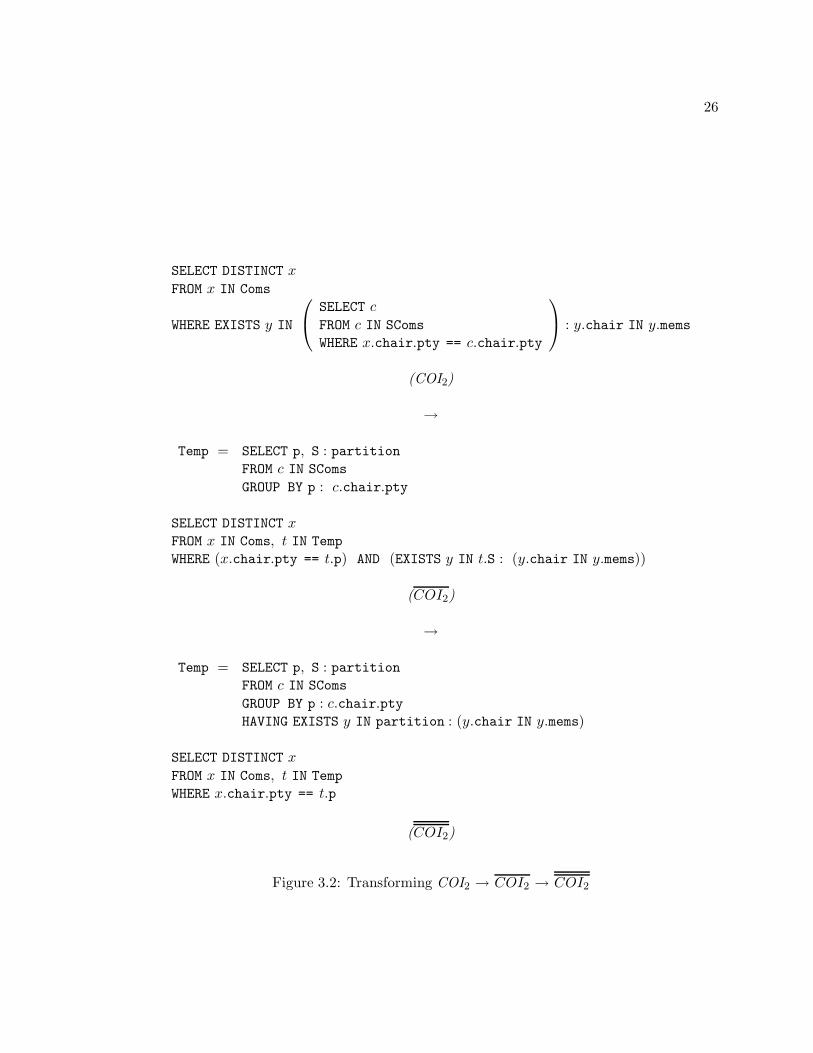
26
SELECT DISTINCT x
FROM x IN Coms
WHERE EXISTS y IN
SELECT c
FROM c IN SComsWHERE x.chair.pty == c.chair.pty
: y.chair IN y.mems
(COI2)
→
Temp = SELECT p, S : partitionFROM c IN SComsGROUP BY p : c.chair.pty
SELECT DISTINCT xFROM x IN Coms, t IN TempWHERE (x.chair.pty == t.p) AND (EXISTS y IN t.S : (y.chair IN y.mems))
(COI2)
→
Temp = SELECT p, S : partitionFROM c IN SComsGROUP BY p : c.chair.ptyHAVING EXISTS y IN partition : (y.chair IN y.mems)
SELECT DISTINCT x
FROM x IN Coms, t IN TempWHERE x.chair.pty == t.p
(COI2)
Figure 3.2: Transforming COI2 → COI2 → COI2

27
C1 = SELECT A1, A2 : partitionFROM V1 IN C2GROUP BY A1 : V1.A3
SELECT DISTINCT V2.A7FROM V2 IN C1, V3 IN C3WHERE (V2.A4 == V3.A1) AND (EXISTS V4 IN V3.A2 : (V4.A5 Op1 V4.A6)
→=
C1 = SELECT A1, A2 : partitionFROM V1 IN C2GROUP BY A1 : V1.A3HAVING EXISTS V4 IN partition : (V4.A5 Op1 V4.A6)
SELECT DISTINCT V2.A7FROM V2 IN C1, V3 IN C3WHERE V2.A4 == V3.A1
Figure 3.3: A Rewrite Rule Justifying COI2 → COI2
To summarize, queries COI1 and COI2 are syntactically similar but semantically distinct.
Further, these two queries are subject to different query rewrites. Query rewrites perform
subexpression identification in part to determine if rewriting can occur. As pattern matching
can only make syntactic distinctions between expressions, code must be used by any non-
trivial query rewrite that rewrites COI2 to COI2 to ensure that COI1 is not affected.
Variables Complicate Query Formulation
In formulating new queries, query rewrites can reuse subexpressions identified in the original
query. But if these subexpressions include free variables, the meanings of these subexpres-
sions may change as a result of their use in a different context. Code is required under these
circumstances to massage subexpressions to ensure that their semantics are preserved.
We illustrate this again with an example. Figure 3.4a shows an equivalent query to COI1(COI1∗) and its rewrite into COI1. This rewrite uses a quantified predicate expression,
x.chair.pty == y.chair.pty

28
SELECT DISTINCT xFROM x IN ComsWHERE EXISTS y IN SComs : ((x.chair IN y.mems) AND (x.chair.pty == y.chair.pty))
(COI1∗)
→
SELECT DISTINCT x
FROM x IN Coms
WHERE EXISTS y IN
SELECT c
FROM c IN SComsWHERE x.chair.pty == c.chair.pty
: x.chair IN y.mems
(COI1)
(a)
SELECT DISTINCT V1FROM V1 IN C1WHERE EXISTS V2 IN C2 : (E1 AND (V3.A1 Op1 V2.A2))
→=
SELECT DISTINCT V1FROM V1 IN C1
WHERE EXISTS V2 IN
SELECT V4
FROM V4 IN C2WHERE V3.A1 Op1 V4.A2
: E1
(b)
Figure 3.4: COI1∗ → COI1 (a) and a Rule to Justify It (b)

29
as a filter condition for a new (inner) subquery:
SELECT c
FROM c IN SComs
WHERE x.chair.pty == c.chair.pty.
This rewrite is useful as it enables COI1∗ to be subsequently rewritten into COI1.
Figure 3.4b shows a rewrite rule expressing this rewrite. Again, this rewrite rule is
overly specific. Any predicate expression can be moved out of a quantifier and into an inner
query; predicate expressions need not be of the form,
V3.A1 Op1 V2.A2
as stipulated by the rule of Figure 3.4b. But if any predicate that is moved includes
occurences of the quantified variable V2 (y), then all occurences of this variables must be
renamed. In this case, y is renamed to c, changing the expression
x.chair.pty == y.chair.pty
to
x.chair.pty == c.chair.pty.
Thus, code is necessary to rename variables appearing in subexpressions used to formu-
late new queries, and more generally, to substitute any expressions (not just variables) for
variables appearing in other expressions.
3.1.2 The Need for a Combinator-Based Query Algebra: Summary
Query rewrites perform two steps in rewriting a query: (1) subexpression identification,
and (2) query formulation. For query rewrites to be expressed as rewrite rules, a query
representation must ensure that subexpressions of the query:
1. can be identified on the basis of their structure (syntax), and
2. have context-independent semantics so that they can be reused without modification
when new queries are formulated.
Variable-based query representations fail to satisfy both criteria. Therefore, query rewrites
expressed over variable-based representations must be fully or partially expressed with code
that analyzes or manipulates the variables appearing in subexpressions. Combinator-based
representations eliminate variables, and in so doing, eliminate the need for this supplemen-
tary code. In the next section, we illustrate this by revisiting the examples presented in
this section in the context of our combinator-based query algebra, KOLA.

30
3.2 KOLA
Variable-based query representations impede the formulation of query rewrites with rewrite
rules. Therefore, we designed the query algebra, KOLA, which is variable-free (combinator-
based).4 More accurately, KOLA is an algebra of functions and predicates, of which query
operators are simply those that apply to or return collections.
KOLA functions and predicates are expressed using combinator primitives whose seman-
tics are predefined, and combinator formers (second-order functions) that produce complex
functions and predicates from simpler ones. Because combinators have no variables, KOLA
avoids the problems that variables introduce. The semantics of a KOLA expression is tied
to its structure and not to the context in which it appears. Therefore KOLA rewrite rules
need no code to assist with subexpression identification or query formulation.
It should be noted that KOLA is a language for optimizers and not users, and KOLA
queries are far more difficult to read than OQL queries. As best as possible, we will assist
the reader in decomposing KOLA queries referring to the definitions that appear in the
coming sections. The reader is advised to trace reductions of KOLA queries as we do in the
next section, until becoming comfortable with the notation and combinator style.
3.2.1 An OQL Query Expressed in KOLA
KOLA is a language for expressing functions and predicates invokable on objects. Invoca-
tion is explicit, with “f ! x” denoting the invocation of function f on object x (returning
an object of any type) and “p ? x” denoting the invocation of predicate p on object x (re-
turning a Bool). The KOLA style of querying is illustrated with a simple query shown in
Figure 3.5. Figure 3.5a shows an OQL query that finds all subcommittees in SComs chaired
by Republicans. Figure 3.5b shows its KOLA equivalent.
The KOLA query of Figure 3.5b includes:
• the primitive identity function, id, which maps every object to itself,
• the complex predicate,
Cp (eq, ‘‘GOP’’) ⊕ (pty ◦ chair)
which is true of a committee if its chair is Republican, and4KOLA resembles AQUA but for its combinator foundation and some other language differences describedin our 1995 DBPL paper [23]. Thus, the name KOLA was coined from the acronym, [K]ind [O]f [L]ike[A]QUA.

31
SELECT cFROM c IN SComsWHERE c.chair.pty == ‘‘GOP’’
(a)
iterate (Cp (eq, ‘‘GOP’’) ⊕ (pty ◦ chair), id) ! SComs
(b)
Figure 3.5: A Simple OQL Query (a) and its KOLA Equivalent (b): Name All Subcommit-tees Chaired by Republicans
• the complex query function,
iterate (Cp (eq, ‘‘GOP’’) ⊕ (pty ◦ chair), id)
which filters a bags of committees for those whose chair is Republican.
We can break these query components down even further as follows.
• pty and chair are primitive functions named for attributes of the Thomas schema
(Table 2.1). For any legislator l,
pty ! l = l.pty
and for any committee c,
chair ! c = c.chair.
Therefore, the semantics of attribute-based primitives such as these depend on the
values of the corresponding attributes for objects populating the database.
• eq is a primitive equality predicate invoked on pairs (denoted by [ , ]) of objects
of the same type. The definition of eq is depends on each type’s definition of equality
(==).
• ◦ is a function composition former that builds a new function that invokes two
other functions in succession. That is, given functions f and g the function f ◦ g has
an operational semantics defined in terms of invocation on an object x:
(f ◦ g) ! x = f ! (g ! x).

32
For example, given a committee x, the semantics of (pty ◦ chair) ! x is revealed by
the reduction below:
(pty ◦ chair) ! x = pty ! (chair ! x)
= pty ! (x.chair)
= x.chair.pty
• Cp ( , ) is a currying predicate former that builds a unary predicate from a binary
predicate by binding the first argument. The semantics of this predicate can be
expressed in terms of any binary predicate p and objects x and y by the equation,
Cp (p, x) ? y = p ? [x, y].
For example, given some string, x, (Cp (eq, ‘‘GOP’’) ? x) has semantics revealed by
the reduction below:
Cp (eq, ‘‘GOP’’) ? x = eq ? [‘‘GOP’’, x]
= ‘‘GOP’’ == x
= x == ‘‘GOP’’
• ⊕ is a combination predicate former that builds a predicate from another predi-
cate and function. Much like function composition, ⊕ first applies the function
to its argument and then tests the predicate on the result. That is, given predicate p
and function f , the predicate (p ⊕ f) has semantics expressible in terms of invocation
on an object x:
(p ⊕ f) ? x = p ? (f ! x).
For example, when invoked on a committee, x,
Cp (eq, ‘‘GOP’’) ⊕ (pty ◦ chair)
has semantics revealed by the reduction below:
(Cp (eq, ‘‘GOP’’) ⊕ (pty ◦ chair)) ? x
= Cp (eq, ‘‘GOP’’) ? ((pty ◦ chair) ! x)
= Cp (eq, ‘‘GOP’’) ? (x.chair.pty)
= x.chair.pty == ‘‘GOP’’

33
• iterate ( , ) is a querying function former that builds a function on bags given a
predicate and a function as inputs. Given any predicate p, function f and bag A, we
have
iterate (p, f) ! A = {|(f ! x)i | xi ∈ A, p ? x|},
such that the expression on the right hand side describes a bag (delimited by “{|”and “|}”) that contains the result of invoking f on all objects in A that satisfy p.
The expression, xi ∈ A indicates that there are i copies of x in A and that i > 0.5
Therefore, the number of elements, x that are in A determines the number of elements,
f ! x that are inserted into the result.
Given these definitions, we can reduce the query expression,
iterate (Cp (eq, ‘‘GOP’’) ⊕ (pty ◦ chair), id) ! SComs
as follows:
iterate (Cp (eq, ‘‘GOP’’) ⊕ (pty ◦ chair), id) ! SComs
= {|(id ! x)i | xi ∈ SComs, (Cp (eq, ‘‘GOP’’) ⊕ (pty ◦ chair)) ? x|}(By the definition of iterate)
= {|xi | xi ∈ SComs, (Cp (eq, ‘‘GOP’’) ⊕ (pty ◦ chair)) ? x|}(By the definition of id)
= {|xi | xi ∈ SComs, x.chair.pty == ‘‘GOP’’|}(By the definitions of Cp, eq, ⊕, ◦, pty and chair.)
Thus, this query returns those committees in SComs whose chair is Republican.
3.2.2 The KOLA Data Model
The KOLA data model assumes a universe of objects, each associated with a type that
defines its interface. A type’s interface can include operators that construct the object, or
observe or mutate its state. A type which includes operators that can mutate an object’s5To keep our notation similar to set comprehension notation, we write x /∈ A when there are no copies
of x in A rather than x0 ∈ A.

34
state is called a mutable type and its objects are mutable objects. Conversely, a type or
object upon which no mutating operations are defined is immutable.
Immutable objects have immutable state, and hence their state reveals their identity.
That is, the integer object 3 has an identity that is inseparable from its value (i.e., all
instances of objects representing the value 3 are equal). On the other hand, mutable objects
should not be compared on the basis of their mutable states as this makes their identities
ephemeral and provokes unintuitive behaviors in any collections that contain them [23].
Rather, mutable objects are assumed to be implemented with immutable, unique object
identifiers (OID’s) that are used by the run-time system to decide if two objects are equal.
In short, KOLA supports both mutable and immutable objects, but mutable objects are
assumed to be compared for equality on the basis of their immutable object identifiers while
immutable objects are compared on the basis of keys.
An informal description of the object types supported by the KOLA data model follows.
Appendix A includes a formal specification of the data model expressed in Larch [46].
• Base Types
The base types supported in KOLA are the immutable types Bool (booleans), Int
(integers), Char (characters), Float (floats) and String (strings). A standard interface
for these types is assumed. Constants of these types have the usual form. As well,
NULL is assumed to be a constant belonging to all types.
• Class Types
KOLA permits queries over collections of objects that are instances of class types. It
is assumed that a class definition defines an interface to which queries have access. In
particular, we assume that queries can invoke the observer operators of objects but
not their mutators or constructors, as queries are assumed to be free of side-effects.6
Finally, it is assumed that observers are unary (attributes).
• Pair Types
A pair type is any type of the form
(t1 × t2)6This is one way that KOLA is less expressive than OQL, as OQL queries can return collections of new
mutable objects. This confuses the issue of optimizer correctness which must then be based on similarityrather than equality of results. We discuss this issue at length elsewhere [18], but have yet to modify KOLAin light of our analysis.

35
such that t1 and t2 are types. Given object x of type t1 (x : t1) and y of type t2
(y : t2), [x, y] is a pair object of type (t1 × t2) ([x, y] : (t1 × t2)). (For example,
the type of [3, Joe] is (Int × Person) assuming that 3 is of type Int and Joe is of
type Person.) Pairs are used to express relationships between objects of potentially
differing types.
• Collection (Bag and Set) Types
For any type t, {|t|} denotes the type of bags whose elements are all of type t. Formally,
a bag A : {|t|} is a function, t → Z such that for any object x : t, A(x) is the number of
occurences of x in A. It is easier to formalize bags and bag operators when bags are
defined in terms of their characteristic functions rather than as collections containing
elements. But sometimes it is more intuitive to use comprehension notation (as used,
for example, in Fegaras and Maier’s work [33]) to reason about the “contents” of a
bag. Therefore, this proposal uses the following shorthand notation:
– for any bag A : {|t|} and expression e : t,
e ∈ A
is shorthand for A(e) > 0 and
ei ∈ A
(for i > 0) is shorthand for A(e) = i.
– for any x1, . . . , xn : t, and positive integers i1, . . . , in,
{|(x1)i1, . . . , (xn)in |}
denotes a bag B : {|t|} containing elements x1, . . . , xn whose count of any element,
y (B(y)) is ∑1≤j≤n, y == xj
ij.
For example, {|(3)1, (−3)2, (2)2, (−3)1|} denotes the bag B such that:
B(−3) = 3,
B(2) = 2,
B(3) = 1,
and for any i not equal to −3, 2 or 3, B(i) = 0. As a further shorthand, we write
{|x1, . . . , xn|}

36
when the element “counts” are implicitly 1. That is,
{|x1, . . . , xn|} = {|(x1)1, . . . , (xn)1|}
– for any bag, A : {|t|}, variable x : t, and expressions, f(x) : u, g(x) : Int and
p(x) : Bool,
{|f(x)g(i) | xi ∈ A, p(x)|}
denotes a bag B : {|u|} containing elements f(x) (for each x ∈ A) whose count of
any element y : u (B(y)) is:
∑xi∈A, y == f(x), p(x)
g(i)
For example, if A = {|3,−3, 2,−3|}. Then
{|(x ∗ x)i | xi ∈ A|}
denotes the bag, B such that
B(4) = 1,
B(9) = 3,
and for any e not equal to 4 or 9, B(e) = 0.
More generally, for bags A1 : {|t1|} . . . An : {|tn|}, variables x1 : t1, . . . xn : tn,
positive integers i1, . . . , in and g(i1, . . . , in), and expressions f(x1, . . . , xn) : u,
p(x1, . . . , xn) : Bool,, and y : u:
{|f(x1, . . . , xn)g(i1,...,in) | (x1)i1 ∈ A1, . . ., (xn)in ∈ An, p(x1, . . . , xn)|}
denotes B : {|u|} such that for all y : u:
B(y) =∑
(x1)i1∈A1,...,(xn)in∈An, y == f(x1,...,xn), p(x1,...,xn)
g(i1, . . . , in)
As an example, suppose that A is defined as above and A′ = {|5, 11, 5, 6|}, then
{|(x + y)ij | xi ∈ A, yj ∈ A′|}

37
denotes the bag, B such that
B(2) = 4,
B(3) = 2,
B(7) = 2,
B(8) = 5,
B(9) = 1,
B(13) = 1,
B(14) = 1,
and for any i not equal to 2, 3, 7, 8, 9, 13 or 14, B(i) = 0.
A set is a special kind of bag whose element counts are either 0 or 1. That is, A is a
set of elements of t if it is a bag of t’s and for all x of type t, A(x) = 1 or A(x) = 0. We
use set comprehension notation in discussing sets. That is, for any x : t, p(x) : Bool
and f(x) : u
{f(x) | x ∈ A, p(x)}is equivalent to
{|(f(x))1 | x ∈ A, p(x)|}
For simplicity, we assume a namespace of identifiers that refer exclusively to stored
collections. All named bags and sets (e.g., Coms, SComs, Lgs etc.) are assumed to be
mutable. However, all bags and sets constructed by KOLA operators are assumed to be
immutable (as in OQL). For queries, the mutable vs. immutable distinction only makes a
difference when deciding if two bags (sets) are equal. Two mutable bags (sets) are equal if
they are the same object (i.e., they have the same object identifier). Two immutable bags
(sets) are equal if they have the same members (modulo equality definitions for the type of
objects they contain). An immutable bag (set) is never equal to a mutable bag (set). Thus,
a query rewrite that rewrites the OQL query,
SELECT x
FROM x IN Coms
to “Coms” is incorrect, as this rewrites a query returning an immutable collection into one
that returns a mutable collection.
3.2.3 KOLA Primitives and Formers
The operators of KOLA are listed in Tables 3.1 (primitives), 3.2 (formers) and 3.3 (query
formers). Each primitive or former is named in the left columns of these tables, and given

38
an operational semantics in the right columns of these tables. These tables are intended
to provide a brief summary of KOLA, and therefore express KOLA’s semantics somewhat
informally. A formal semantics of KOLA expressed in Larch [46] is presented in Appendix A.
Table 3.1: KOLA’s Primitives
KOLA’s primitives functions and predicates are listed in Table 3.1. The operational se-
mantics of these primitives are defined by showing the result of invoking these primitives
on arbitrary objects (x, y and z), integers or floats (i and j), bags (A and B) and bags
containing bags (X).
Primitive functions include the identity function (id) defined over all types, and projec-
tion functions (π1 and π2) and shifting functions (shl and shr) defined over pairs. Integer
and float primitives include an absolute value function (abs) and basic arithmetic operations
(add, sub, mul, and div). The remainder function, mod is also a primitive defined on pairs
of integers only. String functions include an indexing function on (string× integer) pairs to
isolate a character in the string (at) and a string concatenation function on pairs of strings
(concat). Bag primitives include a singleton constructor (single), an element extraction
function (elt), a duplicate removal function (set), a nested bag flattening function (flat),
bag union (uni), intersection (int) and difference (dif) operators over pairs of bags, an
insertion function (ins), and aggregate operators max, min, cnt, sum and avg. KOLA’s
aggregate operators are defined with the same semantics as their corresponding SQL/OQL
aggregates as defined in [28]. Therefore, some of these aggregates (e.g., MAX) return NULL
when invoked on empty collections.
Basic predicate primitives include equality (eq) and inequality (neq) predicates on pairs
of objects of the same type. String, float and integer predicate primitives include the
ordering relations (lt, leq, gt and geq) on pairs of integers and pairs of strings. Not
listed but assumed are schema-dependent functions and predicates based on unary methods
or attributes of objects such as pty and chair. The semantics of such primitives are
determined by the population of the underlying database.
Table 3.2: KOLA’s Basic Formers
KOLA’s basic function and predicate formers are listed in Table 3.2. The operational
semantics of functions and predicates formed with these formers are given in terms of
arbitrary functions (f and g), predicates (p and q), objects (x and y) and bools (b).

39
Description SemanticsBasic Function Primitives
identity id ! x = xprojection (1) π1 ! [x, y] = x
projection (2) π2 ! [x, y] = yshift left shl ! [x, [y, z]] = [[x, y], z]shift right shr ! [[x, y], z] = [x, [y, z]]
Int and Float Function Primitives (i, j integers or floats)absolute value abs ! i = |i|
addition add ! [i, j] = i + j
subtraction sub ! [i, j] = i− jmultiplication mul ! [i, j] = i ∗ j
division div ! [i, j] = i/jmodulus mod ! [i, j] = i mod j (for integers i and j only)
String Function Primitives (s, t strings (arrays of chars))string indexing at ! [s, i] = s[i]
string concatenation concat ! [s, t] = s ‖ t
Bag Function Primitives (A, B bags, X a bag of bags)singleton single ! x = {|x|}
element extraction elt ! {|x|} = xduplicate removal set ! A = {x | x ∈ A}
bag flattening flat ! X = {|xij | xi ∈ A, Aj ∈ X|}bag union uni ! [A, B] = {|x(i+j) | xi ∈ A, xj ∈ B|}
bag intersection int ! [A, B] = {|xmin (i,j) | xi ∈ A, xj ∈ B|}bag difference dif ! [A, B] = {|x(i−j) | xi ∈ A, xj ∈ B, i > j|}
insertion ins ! [x, A] = uni ! [{|x|}, A]Aggregate Primitives (A a bag of integers or floats, u, v integers or floats)maximum max ! A = v s.t. (vi ∈ A ∧ ∀u(uj ∈ A ⇒ v ≥ u))minimum min ! A = v s.t. (vi ∈ A ∧ ∀u(uj ∈ A ⇒ v ≤ u))
count cnt ! A =∑
vi ∈ A(i)
sum sum ! A =∑
vi ∈ A(vi)
average avg ! A = (sum ! A) / (cnt ! A)Basic Predicate Primitives (x and y of type T )
equality eq ? [x, y] = x == y
inequality neq ? [x, y] = x 6= y
String, Float and Int Predicate Primitives (x and y strings or integers)less than lt ? [x, y] = x < y
less than or equal leq ? [x, y] = x ≤ ygreater than gt ? [x, y] = x > y
greater than or equal geq ? [x, y] = x ≥ y
Table 3.1: KOLA Primitives

40
Description SemanticsBasic Function Formers
composition (f ◦ g) ! x = f ! (g ! x)pairing 〈f, g〉 ! x = [f ! x, g ! x]products (f × g) ! [x, y] = [f ! x, g ! y]
constant function Kf (x) ! y = xcurried function Cf (f, x) ! y = f ! [x, y]
conditional function con (p, f, g) ! x ={
f ! x, if p ? x
g ! x, elseBasic Predicate Formers
combination (p ⊕ f) ? x = p ? (f ! x)conjunction (p & q) ? x = (p ? x) ∧ (q ? x)disjunction (p | q) ? x = (p ? x) ∨ (q ? x)negation ∼ (p) ? x = ¬ (p ? x)inverse p−1 ? [x, y] = p ? [y, x]products (p × q) ? [x, y] = (p ? x) ∧ (q ? y)
constant predicate Kp (b) ? x = bcurried predicate Cp (p, x) ? y = p ? [x, y]
Table 3.2: Basic KOLA Formers
Function formers include the function composition former (◦), the function pairing for-
mer (〈 〉) that produces functions that construct pairs, the pairwise product function former
(×) that applies separate functions to separate members of a pair to produce another pair,
the constant function former (Kf) that builds a function that always returns the same result,
the currying function former (Cf) that fixes one argument of a binary (pair) function to
produce a unary function and a conditional function former (con) that applies one of two
functions to its arguments depending on whether a given predicate holds.
KOLA’s predicate formers include the predicate/function combination former (⊕) that
acts much like function composition but producing a predicate, the logic-inspired conjunc-
tion, disjunction and negation predicate formers (&, | and ∼), the predicate inverse former
(−1) that flips its pair argument before applying a given predicate, a pairwise predicate
former (×) that applies distinct predicates to each element of a pair, a constant predicate
former (Kp) that always returns true or always returns false, and a currying predicate former
(Cp) that fixes one of the arguments of a binary predicate to produce a unary predicate.

41
Description SemanticsQuery Function Formers
iteration iterate (p, f) ! A = {|(f ! x)i | xi ∈ A, p ? x|}iteration2 iter (p, f) ! [x, B] = {|(f ! [x, y])j | yj ∈ B, p ? [x, y]|}unnest unnest (f, g) ! A = {|(f ! [x, y])ij | xi ∈ A, yj ∈ (g ! x)|}join join (p, f) ! [A, B] =
{|(f ! [x, y])ij | xi ∈ A, yj ∈ B, p ? [x, y]|}left semijoin lsjoin (p, f) ! [A, B] = {|(f ! x)i | xi ∈ A, p ? [x, B]|}right semijoin rsjoin (p, f) ! [A, B] = {|(f ! y)j | yj ∈ B, p ? [y, A]|}nested join njoin (p, f, g) ! [A, B] =
{[x, g ! {|(f ! y)j | yj ∈ B, p ? [x, y]|}] | x ∈ A}Query Predicate Formers
∃ exists (p) ? A = ∃x (x ∈ A ∧ p ? x)∀ forall (p) ? A = ∀x (x ∈ A ⇒ p ? x)∃ 2 ex (p) ? [x, B] = ∃y (y ∈ B ∧ p ? [x, y])∀ 2 fa (p) ? [x, B] = ∀y (y ∈ B ⇒ p ? [x, y])
Table 3.3: KOLA Query Formers
Table 3.3: KOLA’s Query Formers
A query former is simply a former that constructs a function or predicate on bags. KOLA’s
query formers are listed in Table 3.3. As with tables 3.2, p and q denote predicates, f , g
and h denote functions, and x and y denote function and predicate arguments. As well,
A and B denote bags, X denotes a bag of bags and i and j are integers denoting element
counts.
KOLA’s Function Formers: KOLA’s function query formers include the following:
• iterate (p, f) forms a function on bags, A that behaves much like SQL/OQL’s
SELECT-FROM-WHERE in that it invokes a function (f) on every element of A that
satisfies a predicate (p).
• iter (p, f) forms a function on object, bag pairs, [x, B] that behaves much like
iterate but absorbs the constant x into binary predicate p and binary function f .
• unnest (f, g) forms a function on bags A that returns a bag of elements, f ! [x, y]
for each x drawn from A and each y drawn from (g ! x).

42
• join (p, f) forms a function on pairs of bags, [A, B] that applies f to every pair of
elements, [x, y] such that x is in A, y is in B and the pair [x, y] satisfies p.
• lsjoin (p, f) (short for left semijoin) forms a function on pairs of bags, [A, B] that
applies f to every element of A, x for which [x, B] satisfies p.
• rsjoin (p, f) (short for right semijoin) forms a function on pairs of bags, [A, B] that
applies f to every element of B, y for which [y, A] satisfies p.
• njoin (p, f, g) (short for nested join) forms a function on pairs of bags, [A, B] that
returns a set of pairs, [x, Sx] for each x ∈ A. For a given x, Sx is the result of
invoking g on the collection of (f ! y)’s such that y ∈ B and [x, y] satisfies p. For
example, the SQL query,
SELECT T .c1, agg (T .c2)
FROM T
GROUP BY T .c1
would be translated into the KOLA query,
njoin (eq ⊕ (id × c1), c2, agg) ! [iterate (Kp (true), c1) ! T , T]
such that agg is the KOLA equivalent of SQL aggregate, agg (e.g., COUNT = cnt,
SUM = sum).
Nested joins formed by njoin can also express groupings resulting from joins and
outerjoins. For example, the SQL join query,
SELECT T1.c1, agg (T2.c2)
FROM T1, T2
WHERE T1.c3 == T2.c3
GROUP BY T1.c1
is equivalent to the KOLA query,
njoin (eq ⊕ (π1 × (c1 ◦ π1)), π2, agg) ! [iterate (Kp (true), c1 ◦ π1) ! A, A]
such that
A = join (eq ⊕ (c3 × c3), id × c2) ! [T1, T2].

43
The SQL outerjoin query,
SELECT T1.c1, agg (T .c2)
FROM T1 LEFT JOIN T2 ON T1.c1 == T2.c1
GROUP BY T1.c1
is expressed in similar fashion to GROUP BY queries:
njoin (eq ⊕ (id × c1), c2, agg) ! [iterate (Kp (true), c1) ! T1, T2].
Note that if for some element of t1 ∈ T1 there are no elements t2 ∈ T2 such that
t1.c1 == t2.c2,
then t1.c1 will be paired with (agg ! �) in the result. If agg is an aggregate that
returns NULL when applied to an empty collection (such as MAX), then (agg ! �) is
also NULL and t1.c1 is paired with NULL in the result.
The OQL query below partitions a bag on the basis of predicates p1, . . . pn.
SELECT ∗FROM t IN T
GROUP BY label1 : p1, . . . , labeln : pn.
The result of this query is a set of tuples consisting of n + 1 fields. The first n fields
contain the truth values for the n predicates for a given partition of elements of T
that agree on these values. The (n + 1)th field contains the associated partition of T .
The KOLA version of this query uses functions of the form,
fi = con (pi, Kf (1), Kf (0)),
that when invoked on some object, x, return a 1 or 0 depending on whether predicate
pi (the KOLA translation of pi) is satisfied by x. The partition of T is then based on
equivalence of the bitstring formed by applying functions fi for each 1 ≤ i ≤ n. That
is, given
f = 〈f1, 〈f2, . . . 〈fn−1, fn〉 . . .〉〉,
the KOLA equivalent to the OQL query above is:
njoin (eq ⊕ (id × f), id, id) ! [iterate (Kp (true), f) ! T, T].

44
KOLA’s Predicate Formers: KOLA’s query predicate formers include the following.
• Formers exists (p) and forall (p) form existential and universal quantifier predicates
on bags A that return true if some (all) elements of A satisfy p.
• Formers ex and fa are to exists and forall as iter is to iterate. Like functions
formed with iter, ex (p) and fa (p) are invoked on pairs of the form [x, B], such
that x is absorbed into the predicate, p. The result of invocation depends on whether
any (ex) or all (fa) elements y in B are such that (p ? [x, y]) holds.
3.3 Using a Theorem Prover to Verify KOLA Rewrites
3.3.1 A Formal Specification of KOLA Using LSL
Appendix A contains a formal specification of the KOLA data model and algebra. The
specification is expressed in the Larch algebraic specification language, LSL. LSL permits
the definition of traits, which roughly correspond to abstract data types [72]. LSL includes
a library of basic traits such as Int, Bool, FloatingPoint and String, which are assumed
by the KOLA specification.
KOLA bags (bag [T]) are defined by two traits: BagBasics (which defines bag con-
structors, {} and insert and unary operators on bags) and Bag which defines binary bag
operators (such as union and intersection) These traits introduce the bag constructors,
empty bag: {} : → bag [T],
singleton bag: { } : T → bag [T], and
bag insertion: insert : T, bag [T] → bag [T],
as well as operators,
membership: ∈ : T, bag [T] → Bool,
element difference: − : bag [T], T → bag [T],
bag union: ∪ : bag [T], bag [T] → bag [T],
bag intersection: ∩ : bag [T], bag [T] → bag [T], and
bag difference: − : bag [T], bag [T] → bag [T].
The axioms for these operators assume universally quantified variables A and B of type bag
[T] and x and y of type T. Membership is defined by the axioms:
x ∈ {} = false, and
x ∈ insert (y, A) = (x == y) ∨ (x ∈ A).7

45
Element difference is defined by axioms:
{} − x = {}, and
¬ (x == y) ⇒ (insert (x, A) − y == insert (x, A − y)).
Bag union, intersection and difference are defined by axioms:
(1) {} ∪ B = B,
(2) insert (x, A) ∪ B = insert (x, A ∪ B),
(3) {} ∩ B = {},(4) x ∈ B ⇒ (insert (x, A) ∩ B == insert (x, A ∩ (B − x))) ,
(5) ¬ (x ∈ B) ⇒ (insert (x, A) ∩ B == A ∩ B)
(6) {} − B = {},(7) x ∈ B ⇒ (insert (x, A) − B == A − (B − x)), and
(8) ¬ (x ∈ B) ⇒ (insert (x, A) − B == insert (x, A − B)).
These axioms are typical of algebraic specifications, in that they define each operator over
each constructor. Note that the use of the element difference operator “−” in axioms (4)
and (7) distinguishes the definition of bags from sets. The corresponding axioms for sets
would be:
(4b) x ∈ B ⇒ (insert (x, A) ∩ B == insert (x, A ∩ B)), and
(7b) x ∈ B ⇒ (insert (x, A) − B == A − B).
Note also that the axiom defining the singleton bag, {x}, establishes it as shorthand for
insert (x, {}). Therefore, this constructor does not need to be accounted for in these
axioms.
All function primitives and formers “inherit” the generic Function specification, which
introduces invocation ( ! : fun [T, U], T → U) (for domain type T and range type
U), and function equality ( == : fun [T, U], fun [T, U] → Bool), which is defined
universally for functions f and g (fun [T, U]) by the axiom,
f == g = ∀ x:T (f ! x == g ! x).
Similarly, predicate primitives and formers “inherit” the generic Predicate specification,
which introduces invocation ( ? : pred [T], T → Bool) (for domain type T), and
predicate equality ( == : pred [T], pred [T]→ Bool) which is defined universally
for predicates p and q (pred [T]) by the axiom,
p == q = ∀ x : T (p ? x == q ? x).

46
The axioms defining all KOLA predicate and function primitives and formers are given
in Appendix A. Axioms defining basic primitives and formers (i.e., defining functions and
predicates on arguments that are not collections) resemble the equations shown in Tables 3.1
and 3.2. Query primitives and formers are defined inductively over bag constructors {} and
insert, as in the axioms for
iterate : pred [T], fun [T, U] → fun [bag [T], bag [U]]
shown below:
iterate (p, f) ! {} = {},p ? x ⇒(iterate (p, f) ! insert (x, A) == insert (f ! x, iterate (p, f) ! A)), and
¬ (p ? x) ⇒ (iterate (p, f) ! insert (x, A) == iterate (p, f) ! A).
3.3.2 Proving KOLA Rewrite Rules Using LP
Theorem provers are term rewriters that apply rewrite rules to simplify terms. The LP
theorem prover interprets notation that resembles the notation of logic proofs as operations
to the term rewriting system. LP then gives the following operational interpretations to
these elements of logical proofs:
• the operational interpretation of a conjecture, goal or subgoal is a term,
• the operational interpretation of an axiom is a rewrite rule, and
• the operational interpretation of a proof is a rewrite of a term (conjecture) to the
built-in term true.8
To illustrate the operation of LP, we demonstrate a proof of the KOLA rewrite rule that
pushes projections and selections past unions::
iterate (p, f) ! (A ∪ B) →= (iterate (p, f ) ! A) ∪ (iterate (p, f) ! B).8Larch uses a number of built-in rewrite rules to supplement those that are generated from formal
specifications. For example, Larch has a rewrite rule that rewrites any term of the form
e == e
for some expression e into the term true. Therefore, rewrites of conjectures into the term true are possibleeven when true does not appear as a term in a formal specification, as in the specification of KOLA.

47
%%%%%%%%%%%%%%%%%%%%%%%%%%%%%%%%%%%%%%%%%%%%%%%%%%%%%%%%%%%%proveiterate (p, f) ! (A \U B) =(iterate (p, f) ! A) \U (iterate (p, f) ! B)
..
resume by induction on A % Step 1
% Base Case: Trivial% Trivial Case
resume by induction on B % Step 2
% Base Case: Trivial% Trivial Case
resume by cases p ? u1 % Step 3
% Case 1resume by cases pc ? u % Step 4a
% Case 2resume by cases pc ? u % Step 4b
qed%%%%%%%%%%%%%%%%%%%%%%%%%%%%%%%%%%%%%%%%%%%%%%%%%%%%%%%%%%%%
Figure 3.6: An Example LP Proof Script
As with OQL rules, KOLA rules are expressed with patterns (KOLA queries supplemented
with pattern variables) separated by “→=”. Verification of this rule requires proving the LP
conjecture
iterate (p, f) ! (A \U B) = (iterate (p, f) ! A) \U (iterate (p, f) ! B)
Verification of this conjecture proceeds according to the the proof script shown in Figure 3.69.
To facilitate the tracing of this script, we have numbered the steps that appear in the script
in comments (delimited by %) to the right of each executable statement. Below we trace
the logic behind the proof, and the mechanics of the theorem prover as it processes each
step’s instruction.9We use ASCII notation in presenting inputs to LP (e.g., \U is used instead of ∪, p is used instead of petc.) to emphasize their executable flavor.

48
1. {} \U B --> B2. insert (x, A) \U B --> insert (x, A \U B)3. iterate (p, f) ! {} --> {}4. (p ? x) ::
iterate (p, f) ! insert (x, A) --> insert (f ! x, iterate (p, f) ! A)5. ~(p ? x) ::
iterate (p, f) ! insert (x, A) --> iterate (p, f) ! A
Figure 3.7: Some LP Rewrite Rules Generated from Specification Axioms
The proof begins with the generation of a bank of rewrite rules from the axioms defining
the operators appearing in the proof. For this proof, these axioms generate a bank of rewrite
rules that include those shown in Figure 3.7. As with KOLA’s rewrite rules, LP’s rewrite
rules consist of pairs of patterns (separated by “-->” rather than →= to distinguish them
from KOLA rules). As well, LP’s rules can be conditional — an idea inspiring extensions
to KOLA presented in Chapter 5. Rules 4 and 5 can fire only if the conditions, (p ? x)
and ∼ (p ? x) are respectively satisfied.
Step 1: The proof begins by induction on the collection A. The theorem prover interprets
this instruction by first creating the basis subgoal,
iterate (p, f) ! ({} \U B) ==
(iterate (p, f) ! {}) \U (iterate (p, f) ! B).
This subgoal trivially reduces to true (i.e., is proven) by LP rewrite rules 1 and 3 of
Figure 3.7.
Successful proof of the basis subgoal initiates the addition of a new rewrite rule (corre-
sponding to the induction hypothesis) and the attempted proof of a second subgoal (corre-
sponding to the induction subgoal). For this proof, the induction hypothesis is the rewrite
rule,
iterate (p, f) ! (Ac \U B) -->
(iterate (p, f) ! Ac) \U (iterate (p, f) ! B)
and the induction subgoal is,
iterate (p, f) ! (insert (u, Ac) \U B) ==
(iterate (p, f) ! insert (u, Ac)) \U (iterate (p, f) ! B)

49
Step 2: Induction is again initiated, this time on the collection B in order to prove the
induction subgoal remaining after step 1. The basis subgoal,
iterate (p, f) ! (insert (u, Ac) \U {}) ==
(iterate (p, f) ! insert (u, Ac)) \U (iterate (p, f) ! {})
again reduces to true by rewrite rules 1 and 3 of Figure 3.7. Again, a rewrite rule corre-
sponding to a induction hypothesis is added:
iterate (p, f) ! insert (u, Ac \U Bc) ==
(iterate (p, f) ! insert (u, Ac)) \U (iterate (p, f) ! Bc)
and a new induction subgoal is generated:
iterate (p, f) ! insert (u, Ac \U insert (u1, Bc)) ==
(iterate (p, f) ! insert (u, Ac)) \U (iterate (p, f) ! insert (u1, Bc))
Step 3: The rest of the proof proceeds by cases. A proof by cases requires proving
the current subgoal assuming each case in turn. The assumption of a case is captured
operationally by adding the rewrite rule, p --> true (such that p is the term corresponding
to the case) to the bank of rewrite rules available to the rest of the proof. Step 3 first adds
the rewrite rule,
p ? u1 --> true
to the bank of rewrite rules.
Step 4a: A second case is assumed, adding
p ? u --> true
to the bank of rewrite rules. This rule, taken with the rule generated in step 3 and rule 4 of
Figure 3.7 is sufficient to prove the induction subgoal. Then the converse case is considered,
with
p ? u --> false
added to the bank of rewrite rules in place of the previously added rule. Again, the induction
subgoal is proved using this rule, the rule added in step 3 and rule 5 of Figure 3.7.

50
Step 4b: Having proven the conjecture assuming the case, p ? u1 (Step 3), the converse
case is assumed and
p ? u1 --> false
is added to the bank of rewrite rules replacing the rule added in Step 3. As in Step 4a, a
second case adds
p ? u --> true
and
p ? u --> false
successively to the bank of rewrite rules. The induction subgoal is proven in both cases with
the rewrite rules generated from the case assumptions, and rules 4 and 5 of Figure 3.7. �Proofs such as that for the rewrite rule shown above have been completed for well over
300 KOLA rules. LP proof scripts that execute the operational versions of some of these
proofs are available electronically from the addresses listed in Appendix B.
3.4 Revisiting the “Conflict of Interests” Queries
In this section, we revisit the “Conflict of Interests” queries presented earlier in this chapter
and in Chapter 2. In Section 3.4.1, we show how each OQL query, COI1 (Figure 2.1),
COI1∗ (Figure 3.4), COI1 (Figure 2.2), and COI2, COI2 and COI2 (Figure 3.2), would get
expressed in KOLA. Then in Section 3.4.2, we show how the same set of rules and sequence
of rule applications rewrites KOLA translations of COI1, COI2, and COI1∗ into their final
forms. The point of this section is to show that these rewrites, when expressed over KOLA
query representations, can be expressed without code.
3.4.1 KOLA Translations of the COI Queries
Figure 3.8 shows KOLA translations of the Conflicts of Interests queries of Chapter 2 and
Section 3.1.1. Queries 1–3 in this figure are translations of COI1, COI1∗ and COI1 from
Figures 2.1, 3.4a and 2.2 respectively. Queries 4–6 are translations of queries COI2, COI2,
and COI2 from Figure 3.2. As before, we begin this section begins by tracing the reductions
of these queries to show that they are valid translations of their OQL equivalents.
Queries 1, 2 and 3 of Figure 3.8 are the KOLA translations of OQL queries COI1,
COI1∗ and COI1 (from Figures 2.1, 3.4a and 2.2) respectively. Therefore, each of these

51
1. set ! (iterate (ex (p) ⊕ 〈id, f〉, id) ! Coms)
COIK1 : A KOLA Translation of COI1 (Figure 2.1)
2. set ! (iterate (ex (p & q) ⊕ 〈id, Kf (SComs)〉, id) ! Coms)
COIK1∗: A KOLA Translation of COI1∗ (Figure 3.4a)
3. set ! (join (r & (ex (p) ⊕ (id × π2)), π1) ! [Coms, TempK])
COIK1 : A KOLA Translation of COI1 (Figure 2.2)
4. set ! (iterate (ex (p2) ⊕ 〈id, f〉, id) ! Coms)
COIK2 : A KOLA Translation of COI2 (Figure 3.2)
5. set ! (join (r & (ex (p2) ⊕ (id × π2)), π1) ! [Coms, TempK])
COIK2 : A KOLA Translation of COI2 (Figure 3.2)
6. set ! (join (r, π1) ! [Coms, iterate (p3, id) ! TempK])
COIK2 : A KOLA Translation of COI2 (Figure 3.2)
such that
p ≡ ex (eq) ⊕ 〈chair ◦ π1, mems ◦ π2〉p2 ≡ ex (eq) ⊕ 〈chair ◦ π2, mems ◦ π2〉p3 ≡ exists (ex (eq) ⊕ 〈chair, mems〉) ⊕ π2
q ≡ eq ⊕ ((pty ◦ chair) × (pty ◦ chair))r ≡ eq ⊕ ((pty ◦ chair) × π1)f ≡ iter (q, π2) ◦ 〈id, Kf (SComs)〉
TempK ≡ njoin (eq ⊕ (id × (pty ◦ chair)), id, id) ![iterate (Kf (true), pty ◦ chair) ! SComs, SComs]
Figure 3.8: KOLA Translations of the Conflict of Interests Queries

52
queries returns a set consisting of committees whose chairs are members of a subcommittee
whose chair is from the same party. Queries 4, 5 and 6 of Figure 3.8 translate OQL queries
COI2, COI2 and COI2 from Figure 3.2. Therefore, each of these queries returns a set of
committees whose chairs who belong to a party that includes someone who both chairs
and is a member of the same subcommittee. All of these queries remove duplicates from
intermediate subquery results generated with iterate or join.
These queries are fairly complex, and are easiest to understand when decomposed.
Therefore, we begin by examining some of the common subexpressions that appear in these
queries.
1. The predicate p,
ex (eq) ⊕ 〈chair ◦ π1, mems ◦ π2〉
appears in queries 1, 2 and 3, and is a predicate on committee, subcommittee pairs,
[x, y]. The expression, p ? [x, y] reduces as follows:
(ex (eq) ⊕ 〈chair ◦ π1, mems ◦ π2〉) ? [x, y]
= ex (eq) ? (〈chair ◦ π1, mems ◦ π2〉 ! [x, y])
= ex (eq) ? [(chair ◦ π1) ! [x, y], (mems ◦ π2) ! [x, y]]
= ex (eq) ? [(chair ◦ π1) ! [x, y], mems ! (π2 ! [x, y])]
= ex (eq) ? [chair ! x, mems ! y]
= ex (eq) ? [x.chair, y.mems]
= ∃z : Legislator (z ∈ y.mems ∧ eq ? [x.chair, z])
= ∃z : Legislator (z ∈ y.mems ∧ x.chair == z)
= x.chair ∈ y.mems
Therefore, p ? [x, y] is equivalent to the OQL boolean expression,
x.chair IN y.mems.
2. The predicate p2,
ex (eq) ⊕ 〈chair ◦ π2, mems ◦ π2〉
appears in queries 4 and 5, and is similar to p in that it too is a predicate on committee,
subcommittee pairs, [x, y]. However, p2 ignores x as shown in the reduction below.
(ex (eq) ⊕ 〈chair ◦ π2, mems ◦ π2〉) ? [x, y]

53
= ex (eq) ? (〈chair ◦ π2, mems ◦ π2〉 ! [x, y])
= ex (eq) ? [(chair ◦ π2) ! [x, y], (mems ◦ π2) ! [x, y]]
= ex (eq) ? [(chair ◦ π2) ! [x, y], mems ! (π2 ! [x, y])]
= ex (eq) ? [chair ! y, mems ! y]
= ex (eq) ? [y.chair, y.mems]
= ∃z : Legislator (z ∈ y.mems ∧ eq ? [y.chair, z])
= ∃z : Legislator (z ∈ y.mems ∧ y.chair == z)
= y.chair ∈ y.mems
Therefore, p2 ? [x, y] is equivalent to the OQL boolean expression,
y.chair IN y.mems.
3. The predicate p3,
exists (ex (eq) ⊕ 〈chair, mems〉) ⊕ π2
appears in query 6, and is a predicate on pairs, [p, S], such that p is the name of a
party and S is a set of subcommittees. Reducing p3 ? [p, S], we get:
(exists (ex (eq) ⊕ 〈chair, mems〉) ⊕ π2) ? [p, S]
= exists (ex (eq) ⊕ 〈chair, mems〉) ? (π2 ! [p, S])
= exists (ex (eq) ⊕ 〈chair, mems〉) ? S
= ∃y (y ∈ S ∧ (ex (eq) ⊕ 〈chair, mems〉) ? y)
= ∃y (y ∈ S ∧ ex (eq) ? (〈chair, mems〉 ! y))
= ∃y (y ∈ S ∧ ex (eq) ? [y.chair, y.mems])
= ∃y (y ∈ S ∧ ∃z (z ∈ y.mems ∧ eq ? [y.chair, z]))
= ∃y (y ∈ S ∧ ∃z (z ∈ y.mems ∧ y.chair == z))
= ∃y (y ∈ S ∧ (y.chair ∈ y.mems)).
Thus, p3 ? [p, S], is equivalent to the OQL boolean expression,
EXISTS y IN S : (y.chair IN y.mems).
4. The predicate q,
eq ⊕ ((pty ◦ chair) × (pty ◦ chair))

54
appears in every query in Figure 3.8, and is a predicate on committee, subcommittee
pairs, [x, y]. Reducing q ? [x, y], we get:
(eq ⊕ ((pty ◦ chair) × (pty ◦ chair))) ? [x, y]
= eq ? [(pty ◦ chair) ! x, (pty ◦ chair) ! y]
= eq ? [pty ! (chair ! x), pty ! (chair ! y)]
= eq ? [pty ! (x.chair), pty ! (y.chair)]
= eq ? [x.chair.pty, y.chair.pty]
= x.chair.pty == y.chair.pty
Thus, q ? [x, y], is equivalent to the OQL boolean expression,
x.chair.pty == y.chair.pty.
5. The predicate r,
eq ⊕ ((pty ◦ chair) × π1)
of queries 3, 5 and 6 is similar to q, but is a predicate on nested pairs, [x, [p, S]]
such that x is a committee in Coms, p is the name of a political party and S is a bag
of subcommittees. Reducing r ? [x, [p, S]], we get:
(eq ⊕ ((pty ◦ chair) × π1)) ? [x, [p, S]]
= eq ? (((pty ◦ chair) × π1) ! [x, [p, S]])
= eq ? [(pty ◦ chair) ! x, π1 ! [p, S]]
= eq ? [pty ! (x.chair), p]
= eq ? [x.chair.pty, p]
= x.chair.pty == p
Thus, r ? [x, [p, S]], is equivalent to the OQL boolean expression,
x.chair.pty == p.
6. The function f,
iter (q, π2) ◦ 〈id, Kf (SComs)〉appears in queries 1 and 4, and is a function on committees, x. Reducing f ! x, we
get:
(iter (q, π2) ◦ 〈id, Kf (SComs)〉) ! x

55
= iter (q, π2) ! (〈id, Kf (SComs)〉 ! x)
= iter (q, π2) ! [id ! x, Kf (SComs) ! x]
= iter (q, π2) ! [x, SComs]
= {|(π2 ! [x, c])j | cj ∈ SComs, q ? [x, c]|}= {|cj | cj ∈ SComs, q ? [x, c]|}= {|cj | cj ∈ SComs, x.chair.pty == c.chair.pty|}
Thus, f ! x is equivalent to the OQL query expression,
SELECT c
FROM c IN SComs
WHERE x.chair.pty == c.chair.pty.
7. TempK is a subquery of queries 3, 5 and 6. TempK uses iterate and njoin to generate
the KOLA equivalent of subquery Temp of Figure 2.2. This is illustrated by the
derivation below:
njoin (eq ⊕ (id × (pty ◦ chair)), id, id) !
[iterate (Kp (true), pty ◦ chair) ! SComs, SComs]
= njoin (eq ⊕ (id × (pty ◦ chair)), id, id) !
[{|((pty ◦ chair) ! c)i | ci ∈ SComs, Kp (true) ? c|}, SComs]
= njoin (eq ⊕ (id × (pty ◦ chair)), id, id) !
[{|(pty ! (chair ! c))i | ci ∈ SComs, Kp (true) ? c|}, SComs]
= njoin (eq ⊕ (id × (pty ◦ chair)), id, id) !
[{|(pty ! (c.chair))i | ci ∈ SComs|}, SComs]
= njoin (eq ⊕ (id × (pty ◦ chair)), id, id) !
[{|(c.chair.pty)i | ci ∈ SComs|}, SComs]
= {[c.chair.pty, Sc] | c.chair.pty ∈ {|(c.chair.pty)i | ci ∈ SComs|}} s.t.
Sc = id ! {|(id ! s)j | sj ∈ SComs, (eq ⊕ (id × pty ◦ chair)) ? [p, s]|}

56
= {|sj | sj ∈ SComs, (eq ⊕ (id × (pty ◦ chair))) ? [p, s]|}= {|sj | sj ∈ SComs, eq ? ((id × (pty ◦ chair)) ! [p, s])|}= {|sj | sj ∈ SComs, eq ? [id ! p, (pty ◦ chair) ! s]|}= {|sj | sj ∈ SComs, eq ? [id ! p, pty ! (chair ! s)]|}= {|sj | sj ∈ SComs, eq ? [p, s.chair.pty]|}= {|sj | sj ∈ SComs, p == s.chair.pty|}
= {[c.chair.pty, Sc] | ci ∈ SComs}s.t. Sc = {|sj | sj ∈ SComs, c.chair.pty == s.chair.pty|}
Therefore, this subquery returns a set of pairs, [p, S], such that p is the name of a
party affiliated with some subcommittee’s chair and S is the bag of all subcommittees
chaired by someone from that party. In other words, TempK is equivalent to the OQL
query,SELECT p, S : partition
FROM c IN SComs
GROUP BY p : c.chair.pty
Using the subexpressions above, a description of each of the queries of Figure 3.8 follows.
COIK1 (1):
Predicates p, q and f are all subexpressions of COIK1 ’s subpredicate, (ex (p) ⊕ 〈id, f〉),
which when invoked on a committee x ∈ Coms is equivalent to the OQL expression,
EXISTS y IN
SELECT c
FROM c IN SComs
WHERE x.chair.pty == c.chair.pty
: (x.chair IN y.mems).
as is demonstrated by the derivation below:
(ex (p) ⊕ 〈id, f〉) ? x = ex (p) ? (〈id, f〉 ! x)
= ex (p) ? [x, f ! x]
= ex (p) ? [x, Sx]
s.t. Sx = {|cj | cj ∈ SComs, x.chair.pty == c.chair.pty|}= ∃y (y ∈ Sx ∧ p ? [x, y])
= ∃y (y ∈ Sx ∧ x.chair ∈ y.mems)

57
Therefore, the iterate subquery generates the collection derived below,
iterate (ex (p) ⊕ 〈id, f〉, id) ! Coms
= {|(id ! x)i | xi ∈ Coms, (ex (p) ⊕ 〈id, f〉) ? x|}= {|xi | xi ∈ Coms, (ex (p) ⊕ 〈id, f〉) ? x|}= {|xi | xi ∈ Coms, ∃y (y ∈ Sx ∧ x.chair ∈ y.mems)|}
Removing duplicates from this result leaves,
{x | x ∈ Coms, ∃y (y ∈ Sx ∧ x.chair ∈ y.mems)}
which is the same result returned by the OQL query, COI1.
COIK1∗ (2):
COIK1∗ is similar to COIK
1 in that it performs duplicate elimination on the result of an
iterate subquery, and contains the same subpredicates, p and q. But this query differs
from COIK1 in that it does not generate an intermediate collection (Sx) for each x ∈ Coms.
Instead, the existential predicate (ex (p & q)) searches SComs for some subcommittee y
that with x satisfies both p and q. Therefore, when invoked on a committee x ∈ Coms, this
predicate is equivalent to the OQL expression,
EXISTS y IN SComs : ((x.chair IN y.mems) AND (x.chair.pty == y.chair.pty)),
as shown by the derivation below:
(ex (p & q) ⊕ 〈id, Kf (SComs)〉) ? x
= ex (p & q) ? (〈id, Kf (SComs)〉 ! x)
= ex (p & q) ? [id ! x, Kf (SComs) ! x]
= ex (p & q) ? [x, SComs]
= ∃y (y ∈ SComs ∧ (p & q) ? [x, y])
= ∃y (y ∈ SComs ∧ p ? [x, y] ∧ q ? [x, y])
= ∃y (y ∈ SComs ∧ x.chair ∈ y.mems ∧ x.chair.pty == y.chair.pty)
Thus, the iterate subquery of COIK1∗ returns:
iterate (ex (p & q) ⊕ 〈id, Kf (SComs)〉, id) ! Coms

58
= {|(id ! x)i | xi ∈ Coms, (ex (p & q) ⊕ 〈id, Kf (SComs)〉) ? x|}= {|xi | xi ∈ Coms, (ex (p & q) ⊕ 〈id, Kf (SComs)〉) ? x|}
={|xi | xi ∈ Coms
∃y (y ∈ SComs ∧ x.chair ∈ y.mems ∧ x.chair.pty == y.chair.pty)|}.
Removing duplicates from this result leaves,
{x | x ∈ Coms, ∃y (y ∈ SComs ∧ x.chair ∈ y.mems ∧ x.chair.pty == y.chair.pty)},
which is also the result of the OQL query, COI1∗.
COIK1 (3):
COIK1 computes the same result as COIK
1 and COIK1∗, but using join in its sub-
query rather than iterate. The join is of Coms and TempK , and uses predicates r and
(ex (p) ⊕ (id × π2)). The latter complex predicate is a predicate on nested pairs
[x, [p, S]]
(such that x ∈ Coms and [p, S] ∈ TempK) that is equivalent to the OQL boolean expression,
EXISTS y IN S : (x.chair IN y.mems)
as illustrated by the derivation below:
(ex (p) ⊕ (id × π2)) ? [x, [p, S]] = ex (p) ? ((id × π2) ! [x, [p, S]])
= ex (p) ? [id ! x, π2 ! [p, S]]
= ex (p) ? [x, S]
= ∃y (y ∈ S ∧ p ? [x, y])
= ∃y (y ∈ S ∧ x.chair ∈ y.mems)
Therefore, the result of the join is a collection of committees whose chairs are members of
a subcommitee chaired by someone from the same party, as illustrated by the derivation:
join (r & (ex (p) ⊕ (id × π2)), π1) ! [Coms, TempK]
={|(π1 ! [x, [p, S]])ij |
xi ∈ Coms, [p, S]j ∈ TempK, (r & (ex (p) ⊕ (id × π2))) ? [x, [p, S]]|}
= {|xij | xi ∈ Coms, [p, S]j ∈ TempK, (r & (ex (p) ⊕ (id × π2))) ? [x, [p, S]]|}

59
= {|xi | xi ∈ Coms, [p, S] ∈ TempK , (r & (ex (p) ⊕ (id × π2))) ? [x, [p, S]]|}
={|xi | xi ∈ Coms, [p, S] ∈ TempK ,
r ? [x, [p, S]], (ex (p) ⊕ (id × π2)) ? [x, [p, S]]|}After duplicate elimination, this becomes,
{x | x ∈ Coms, [p, S] ∈ TempK , r ? [x, [p, S]], (ex (p) ⊕ (id × π2)) ? [x, [p, S]]}.
Because r ? [x, [p, S]] is true if
x.chair.pty == p
and (ex (p) ⊕ (id × π2)) ? [x, [p, S]] is true if
∃y (y ∈ S ∧ x.chair ∈ y.mems),
this expression reduces to
{x | x ∈ Coms, [p, S] ∈ TempK , x.chair.pty == p, ∃y (y ∈ S ∧ x.chair ∈ y.mems)}
which is also what is returned by the OQL query, COI1.
COIK2 (4):
Query COIK2 (4) is almost identical to query COIK
1 (1) but using the predicate p2 rather
than p. Given a committee x ∈ Coms, ((ex (p2) ⊕ 〈id, f〉) ? x) is equivalent to the OQL
expression,
EXISTS y IN
SELECT c
FROM c IN SComs
WHERE x.chair.pty == c.chair.pty
: y.chair IN y.mems
as is revealed by the derivation below:
(ex (p2) ⊕ 〈id, f〉) ? x
= ex (p2) ? [id ! x, f ! x]
= ex (p2) ? [x, Sx]
such that Sx = {|ci | ci ∈ SComs, x.chair.pty == c.chair.pty|}= ∃y (y ∈ Sx ∧ p2 ? [x, y])
= ∃y (y ∈ Sx ∧ y.chair ∈ y.mems)

60
Therefore, the iterate subquery of this query generates the collection,
{|xi | xi ∈ Coms, ∃y (y ∈ Sx ∧ y.chair ∈ y.mems)|}.
Removing duplicates from this result leaves,
{x | x ∈ Coms, ∃y (y ∈ Sx ∧ y.chair ∈ y.mems)},
which is the same result returned by the OQL query, COI2.
COIK2 (5):
Query COIK2 (5) is almost identical to query COIK
1 (3) but for its use of p2 rather than
p. The join predicate for this query consists of r and (ex (p2) ⊕ (id × π2)). The latter
predicate on nested pairs [x, [p, S]] (such that x is in Coms and [p, S] is in TempK) is
equivalent to the OQL expression
EXISTS y IN S : (y.chair IN y.mems),
as is revealed by the derivation below:
(ex (p2) ⊕ (id × π2)) ? [x, [p, S]] = ex (p2) ? ((id × π2) ! [x, [p, S]])
= ex (p2) ? [id ! x, π2 ! [p, S]]
= ex (p2) ? [x, S]
= ∃y (y ∈ S ∧ p2 ? [x, y])
= ∃y (y ∈ S ∧ y.chair ∈ y.mems).
Therefore, the result of the join is a collection of committees whose chairs belong to a party
which also includes someone who both chairs and is a member of some subcommitee:
join (r & (ex (p2) ⊕ (id × π2)), π1) ! [Coms, TempK]
= {|xij | xi ∈ Coms, [p, S]j ∈ TempK , (r & (ex (p2) ⊕ (id × π2))) ? [x, [p, S]]|}= {|xi | xi ∈ Coms, [p, S] ∈ TempK, (r & (ex (p2) ⊕ (id × π2))) ? [x, [p, S]]|}
={|xi | xi ∈ Coms, [p, S] ∈ TempK ,
r ? [x, [p, S]], (ex (p2) ⊕ (id × π2)) ? [x, [p, S]]|}
After duplicate elimination, this becomes,
{x | x ∈ Coms, [p, S] ∈ TempK , r ? [x, [p, S]], (ex (p2) ⊕ (id × π2)) ? [x, [p, S]]}.

61
Because r ? [x, [p, S]] is true if
x.chair.pty == p
and (ex (p2) ⊕ (id × π2)) ? [x, [p, S]] is true if
∃y (y ∈ S ∧ y.chair ∈ y.mems),
this expression reduces to
{x | x ∈ Coms, [p, S] ∈ TempK, x.chair.pty == p, ∃y (y ∈ S ∧ y.chair ∈ y.mems)},
which is what is also returned by the OQL query, COI2.
COIK2 (6):
Query COIK2 (6) generates TempK as a subquery result as in COIK
2 , but then filters this
result before proceeding with the join. The filtering subquery uses the predicate p3 which is
a predicate on pairs from TempK [p, S] that is equivalent to the OQL boolean expression,
EXISTS y IN S : (y.chair IN y.mems)
as illustrated by the derivation below:
(exists (ex (eq) ⊕ 〈chair, mems〉) ⊕ π2) ? [p, S]
= exists (ex (eq) ⊕ 〈chair, mems〉) ? (π2 ! [p, S])
= exists (ex (eq) ⊕ 〈chair, mems〉) ? S
= ∃y (y ∈ S ∧ (ex (eq) ⊕ 〈chair, mems〉) ? y)
= ∃y (y ∈ S ∧ ex (eq) ? (〈chair, mems〉 ! y))
= ∃y (y ∈ S ∧ ex (eq) ? [y.chair, y.mems])
= ∃y (y ∈ S ∧ ∃z (z ∈ y.mems ∧ eq ? [y.chair, z]))
= ∃y (y ∈ S ∧ ∃z (z ∈ y.mems ∧ y.chair == z))
= ∃y (y ∈ S ∧ (y.chair ∈ y.mems)).
Therefore, the result of filtering TempK is the set of party, subcommittee collection pairs
([p, S]) such that for some subcommittee in c ∈ S, c’s chair is also a member of c. The
intermediate result returned as a result of join is therefore:
join (r, π1) ! [Coms, iterate (p3, id) ! TempK]

62
= join (r, π1) ! [Coms, {|(id ! [p, S])j | [p, S]j ∈ TempK, p3 ? [p, S]|}]= join (r, π1) ! [Coms, {[p, S] | [p, S] ∈ TempK , p3 ? [p, S]}]= {|(π1 ! [x, [p, S]])i | xi ∈ Coms, [p, S] ∈ TempK , p3 ? [p, S], r ? [x, [p, S]]|}= {|xi | xi ∈ Coms, [p, S] ∈ TempK , p3 ? [p, S], r ? [x, [p, S]]|}.
Because r ? [x, [p, S]] is true if
x.chair.pty == p
and p3 ? [p, S] is true if
∃y (y ∈ S ∧ (y.chair ∈ y.mems)),
this expression reduces to,
{|xi | xi ∈ Coms, [p, S] ∈ TempK, ∃y (y ∈ S ∧ (y.chair ∈ y.mems)), x.chair.pty == p|},
which is also what is returned by the OQL query, COI2.
3.4.2 A Rule Set for Rewriting the COI Queries
Figure 3.9 shows a set of KOLA rewrite rules that can be fired in the same sequence to
rewrite:
• COIK1 → COIK
1∗ → COIK1 , and
• COIK2 → COIK
2 → COIK2 .
(The KOLA transformation chain is slightly different than that presented for the OQL
versions of these queries in that COIK1 is transformed into COIK
1∗ rather than vice-versa.)
The sequence used for these rules is:
1, 2, 3, 4, 5, 6, 5−1, 7, 5, 8, 9
such that 5−1 indicates that rule 5 is fired in right-to-left fashion. For the purposes of
discussion, this sequence can be broken down into four subsequences.10 To show the effects of
firing these rules, we illustrate by tracing the rewrite of query COIK2 (Query 4 of Figure 3.8)
first into query COIK2 (5) and then into COIK
2 (6). The steps of this query rewrite are
shown in Figure 3.10 and summarized below.10These rewrites could instead be expressed with four rules (one for each subsequence), but these four
rules would be very complex and would make the specification of the rewrite harder to understand andverify. Such complex rules also hide the fact that the simpler rules have general applicability (rules 4, 5and 7 being the most obvious in this example). Thus, it was decided to keep rules as simple as possibleand to group rules into complex rewrites using COKO, as will be discussed in Section 4.

63
(1) ex (p) ⊕ 〈id, iter (q, π2) ◦ 〈id, Kf (B)〉〉 →= ex (q & p) ⊕ 〈id, Kf (B)〉(2) set ! (iterate (ex (p) ⊕ 〈id, Kf (B)〉, f) ! A) →= set ! (join (p, f ◦ π1) ! [A, B])
(3) set ! (join (q & p, h ◦ π1) ! [A, B]) →=set ! (join (r & (ex (p) ⊕ (id × π2)), h ◦ π1) ! [A, T])
such thatq = eq ⊕ (f × g)r = eq ⊕ (f × π1)T = njoin (eq ⊕ (id × g), id, id) ! [iterate (Kp (true), g) ! B, B]
(4) 〈f ◦ h, g ◦ h〉 →= 〈f, g〉 ◦ h
(5) p ⊕ (f ◦ g) →= (p ⊕ f) ⊕ g
(6) ex (p ⊕ π2)→= exists (p) ⊕ π2
(7) π2 ◦ (f × g) →= g ◦ π2
(8) join (p & (q ⊕ π2), f) ! [A, B]→= join (p, f) ! [A, iterate (q, id) ! B]
(9) id ◦ f→= f
Figure 3.9: Rewrite Rules For the Query Rewrites of the “Conflict of Interests” Queries
Firing Rule 1: Rule 1 pulls a predicate (q) out of an inner query (iter (q, π2)) and into
the existential quantifier, ex. Matching rule 1 with COIK2 binds pattern variables p and q
to KOLA predicates p2 and q. Rewriting then absorbs the predicate q in iter (q, π2) into
the existentially quantified predicate, resulting in ex (q & p2). In short, the result of firing
this rule on COIK2 is a KOLA query equivalent to the OQL query,
SELECT DISTINCT x.chair
FROM x IN Coms
WHERE EXISTS y IN SComs : ((y.chair ∈ y.mems) AND (x.chair.pty == y.chair.pty)).
Firing Rules 2 and 3: Rules 2 and 3 together transform the query resulting from the
previous step into COIK2 . Rule 2 fires on queries matching the head pattern
set ! (iterate (ex (p) ⊕ 〈id, Kf (B)〉, f ) ! A).
This pattern characterizes nested OQL and SQL queries whose WHERE clause contains a
correlated membership or existence predicate (p). Once fired, Rule 2 transforms such queries
into the form,
set ! (join (p, f ◦ π1) ! [A, B]),

64
set ! (iterate (ex (p2) ⊕ 〈id, f〉, id) ! Coms)
p2 ≡ ex (eq) ⊕ 〈chair ◦ π2, mems ◦ π2〉q ≡ eq ⊕ ((pty ◦ chair) × (pty ◦ chair))f ≡ iter (q, π2) ◦ 〈id, Kf (SComs)〉
1→ set ! (iterate (ex (q & p2) ⊕ 〈id, Kf (SComs)〉, id) ! Coms)
2→ set ! (join (q & p2, id ◦ π1) ! [Coms, SComs])
3→ set ! (join (q & p2, id ◦ π1) ! [Coms, TempK])
TempK ≡ njoin (eq ⊕ (id × (pty ◦ chair)), id, id) ![iterate (Kp (true), pty ◦ chair) ! SComs, SComs]
p2 ≡ ex (ex (eq) ⊕ 〈chair ◦ π2, mems ◦ π2〉) ⊕ (id × π2)q ≡ eq ⊕ ((pty ◦ chair) × π1)
(a) The first transformation of COIK2 to COIK
2
4→ set ! (join (q & p2, id ◦ π1) ! [Coms, TempK])p2 ≡ ex (ex (eq) ⊕ (〈chair, mems〉 ◦ π2)) ⊕ (id × π2)
5→ set ! (join (q & p2, id ◦ π1) ! [Coms, TempK])p2 ≡ ex (ex (eq) ⊕ 〈chair, mems〉 ⊕ π2) ⊕ (id × π2)
6,5−1
→ set ! (join (q & p2, id ◦ π1) ! [Coms, TempK])p2 ≡ exists (ex (eq) ⊕ 〈chair, mems〉) ⊕ (π2 ◦ (id × π2))
7,5→ set ! (join (q & p2, id ◦ π1) ! [Coms, TempK])p2 ≡ exists (ex (eq) ⊕ 〈chair, mems〉) ⊕ π2 ⊕ π2
8→ set ! (join (q, id ◦ π1) ! [Coms, iterate (p3, id) ! TempK])
TempK ≡ njoin (eq ⊕ (id × (pty ◦ chair)), id, id) ![iterate (Kp (true), pty ◦ chair) ! SComs, SComs]
p3 ≡ exists (ex (eq) ⊕ 〈chair, mems〉) ⊕ π2
q ≡ eq ⊕ ((pty ◦ chair) × π1)
9→ set ! (join (q, π1) ! [Coms, iterate (p3, id) ! TempK])
(b) The second transformation of COIK2 to COIK
2
Figure 3.10: Transforming COIK2 → COIK
2 → COIK2

65
thus eliminating the nesting by eliminating the existential predicate former, ex, and replac-
ing it with a join. Thus, this rule generalizes the Type N and Type J query transformations
of Kim [63].
Rule 3 is the most complex rule in this rule set. It fires on queries matching the head
pattern,
set ! (join (q & p, h ◦ π1) ! [A, B])
such that q = eq ⊕ (f × g). Queries matching this pattern return
{h ! a | a ∈ A, b ∈ B, f ! a == g ! b, p ? [a, b]}
as their result. What is noteworthy is that an element, (h ! a) only figures into the result
if there exists some b ∈ B such that f ! a == g ! b and p ? [a, b]. The idea behind rule
3 is to group elements of B by their values for (g ! b) so that the comparison,
f ! a == g ! b
need not be made for each b ∈ B but instead for each unique value of (g ! b). This grouping
is expressed with the body pattern subexpression,
T = njoin (eq ⊕ (id × g), id, id) ! [iterate (Kp (true), g) ! B, B]
that returns the grouped result,
{[g ! b, Sb] | b ∈ B}
such that
Sb = {|(b2)i | (b2)i ∈ B, g ! b == g ! b2|}.That is, this subquery produces a set of pairs, [g ! b, Sb] such that Sb is the subcollection
of B whose elements have the same value for g as b.
The entire body pattern of rule 3 is:
set ! (join (r & (ex (p) ⊕ (id × π2)), h ◦ π1) ! [A, T])
such that r = eq ⊕ (f × π1). Queries rewritten to this form perform a join of A and T ,
and for each pair [a, [g ! b, Sb]] such that a ∈ A and [g ! b, Sb] ∈ T : determines if:
• f ! a == g ! b, and
• ∃ b2 ∈ Sb (p ? [a, b2]).
Finally, duplicates are removed from the result of this join. The result of firing these two
rules on COIK2 is COIK
2 .

66
Firing Rules 4, 5, 6, 5−1, 7 and 5: These rules are fired on the predicate p2 of COIK2 .
The effect is to normalize the predicate to make it of the form, p ⊕ π2 for some predicate
p. This sequence prepares it for the predicate pushdown rule, 8b.
When applied to COIK2 , rule 4 factors the function π2 from the pair function,
〈chair ◦ π2, mems ◦ π2〉,
leaving
〈chair, mems〉 ◦ π2.
Rules 5, 6, 5−1, 7 and 5 again continue to factor π2 from p2, leaving a predicate, p2 ⊕ π2
such that
p2 = exists (ex (eq) ⊕ 〈chair, mems〉) ⊕ π2.
On the other hand, rule 4 fails to fire on COIK1 ’s corresponding subfunction,
〈chair ◦ π1, mems ◦ π2〉.
The other rules that continue to factor π2 out of p (6 and 7) fail to fire also.
Firing Rule 8: This rule identifies the join predicate (p) that is a predicate on the second
argument to the join, and pushes this predicate onto a selection over this second argument.
Thus, the firing of this rule after the normalizing steps of the previous subsequence of rules
transforms COIK2 into COIK
2 . This rule has no effect on COIK1 because this query was not
normalized by the previous set of rule firings,
Firing Rule 9: Finally, rule 9 simplifies the data function of the join, rewriting id ◦ π1
to π1.
3.5 Discussion
3.5.1 The Expressive Power of KOLA
There are downsides to using KOLA as a query representation, but a lack of expressive
power for denoting queries is not one of them. Combinators can appear to lack expressivity
to those who first use them, but the right set of combinators can have rich expressive power.
For example, Schonfinkel [82] established that three combinators (S, K and I) were all that
were required as an alphabet for a free algebra over which one could translate all of the
lambda calculus. (It even was shown later that I was unnecessary.) Within the context of

67
querying, the rich expressivity of KOLA has been established via the design, correctness
proof and implementation of a translator from a set and bag based subset of OQL to KOLA.
This translator is described in Chapter 6.
3.5.2 Addressing the Downsides of KOLA
KOLA Query Representations Are Large
KOLA query representations tend to be larger than their variable-based counterparts (as
measured in parse tree nodes). The size increase is up to a factor of m where m is a
measure of how nested the query is.11 Intuitively, combinator representations are bigger
because functions can require expression with several parse tree nodes, whereas variable
referencces (which they replace) always require just one node. Deeply nested queries can
be especially problematic because variables that are used long after they are declared will
be replaced by functions that are long compositions of projection functions (π1 and π2)
that probe the nested pair data structures that replace the variable’s implicitly constructed
environment.
The representation size issue has been a major concern to the functional programming
community’s effort to use combinators internally to represent functional programs within a
compiler. One solution applied to this problem is to add combinators to the representation
language at the expense of redundancy. Also, a solution has been proposed that has special-
purpose combinators (supercombinators) generated on-the-fly [52].
The supercombinator approach has little practical benefit for querying given that query
rewriting relies on the existence of a fixed set of query operators. But queries tend to be
smaller than programs, and thus such drastic solutions may not be required. We could
get around the problem of having large representations for deeply nested queries by adding
special purpose environment accessing combinators (e.g., π3, π4, . . .) to make the increase in
representation size effectively linear in the size of the original query. But as yet, we haven’t
come across queries that have produced representations that were too large for our system.
The potential modification of KOLA brings up another philosophical issue, which is that
this thesis does not argue for KOLA as the ideal query algebra, but rather for the benefits of
(any) well-designed combinator-based query algebra. KOLA has been and continues to be
plastic – operators are added, removed and modified regularly as new insights are gleaned
into the optimization process. Thus, the potential addition of combinators (such as π3) will11More precisely, m is the maximum number of variables that ever appear in an environment at one time
while evaluating the variable-based query.

68
not compromise our position. We fully expect KOLA to live and grow.
KOLA Requires More Rules than Variable-Based Representations
The other downside to KOLA specifically, and combinator-based query algebras in general,
is the apparent need for multiple rules to express desired transformations. In some ways, this
problem is self-induced. KOLA rules are purposely kept as small as possible to make them
more likely to be reused and understood. But optimizers that are left on their own to choose
a sequence in which to apply multiple rules to perform a single complex transformation are
greatly handicapped when there is an explosion in the number of rules to consider.
As we saw in Section 3.4.2, a fixed sequence of rule applications (perhaps with some rules
applied conditionally) can express a complex transformation for a large class of queries. This
makes a specific sequence of rule firings resemble a theorem prover script that guides normal-
ization of one expression into another to establish that the two expressions are equivalent.
This similarity reveals a serendipitous detail of this thesis work. Theorem prover verifiabil-
ity inspired KOLA, but actually working with a theorem prover and seeing how it operated
motivated COKO, our language for “programming” KOLA rule firing scripts. COKO is
discussed in the next section.
3.6 Chapter Summary
In order to use a theorem prover to verify query rewrites, rewrites must be expressed
declaratively, as in rewrite rules of term rewriting systems. In practice however, query
rewrites get expressed with code, or with rewrite rules supplemented with code.
Query rewrites perform two tasks: (1) subexpression identification identifies relevant
subexpressions of a query, and (2) query formulation constructs new query expressions
from the identified subexpressions. These two steps are captured within standard pattern
matching by actions that use head and body patterns of a rule respectively. But pattern
matching is insufficient for expressing query rewrites when the underlying query represen-
tation is variable-based. The problem is that an expression can contain free variables, which
make its semantics dependent on the context in which it appears. Context-dependent se-
mantics makes subexpression identification require context analysis, and query formulation
require massaging of subexpressions to ensure that their semantics are preserved when used
in a new query. Neither of these actions can be expressed with rule patterns, and therefore
in practice, they get expressed with code.

69
As variables are the problem, our solution was to remove the variables. We have intro-
duced the combinator-based query algebra, KOLA, which expresses functions and predicates
as primitives or as the result of instantiating formers with other functions and predicates.
This approach made it possible to express query rewrites that had been problematic to
express over variable-based representations, in a purely declarative fashion.
Chapter 4
COKO: Complex Query Rewrites
Our KOLA work only partially explains the reason why, in practice, query rewrites get
expressed with code. Rewrite rules are inherently “small” in their operation. They are
well-suited for expressing simple rewrites, such as ones that change the order of arguments
to a join or push selections past joins. But some query rewrites are too complex to be
expressed with rewrite rules, regardless of the underlying query representation. For exam-
ple, a rewrite to convert Boolean expressions to conjunctive normal form (CNF) cannot be
expressed with a rewrite rule because patterns are too constraining to capture its general-
ity. (All boolean expressions can be transformed into CNF.) Instead, this rewrite is more
appropriately described algorithmically. In this chapter, we introduce a language, COKO,1)
for specifying complex query rewrites such as CNF, in a manner that permits verification
with a theorem prover.
A COKO specification of a query rewrite (a transformation) consists of two parts:
1. a set of KOLA rewrite rules, and
2. a firing algorithm that specifies how the KOLA rewrite rules are to be fired.
Code is confined to firing algorithms that specify the order in which KOLA rewrite rules
are fired, the query subexpressions on which rules are fired and the conditions that must
be satisfied for firing to occur. Code is not used to rewrite queries. Instead, rewriting
occurs only by firing KOLA rewrite rules. Therefore, a COKO transformation is correct if
each of the KOLA rewrite rules it fires is correct. We showed in Chapter 3 that a theorem
prover can verify KOLA rewrite rules. By implication, a theorem prover can verify COKO
transformations also.1COKO is an acronym for [C]ontrol [O]f [K]OLA [O]ptimizations.
70

71
This work generalizes and extends KOLA. COKO transformations behave like rewrite
rules in that they can be fired and can succeed or fail as a result. Therefore, the set of
“rules” maintained by a rule-based optimizer could include KOLA rules to express simple
query rewrites, and COKO transformations to express complex query rewrites. COKO
transformations are also built from KOLA rules. By grouping sets of KOLA rewrite rules
into COKO transformations, one can control the number of derivations produced by a rule-
based optimizer. Further, the modular approach of expressing complex transformations in
terms of simpler rewrite rules simplifies reasoning about the meanings of rewrites, just as
expressing complex KOLA queries in terms of simpler functions simplified reasoning about
the meanings of queries.
We begin this chapter in Section 4.1 by describing why COKO is necessary, and why
general purpose programming languages such as C do not satisfy our goal of expressing com-
plex query rewrites in a manner permitting verification with a theorem prover. We then
introduce COKO in Section 4.2 with three example transformations that convert KOLA
predicates into CNF. These examples also show how firing algorithms can determine the
performance of query rewriting.2 We discuss COKO’s language of firing algorithms fully
in Section 4.3. Then in Sections 4.4, 4.5, and 4.6 we demonstrate the expressive power
of COKO by showing how we were able to specify a number of complex, yet useful query
rewrites. These rewrites include a normalization (SNF) to identify subpredicates of a bi-
nary predicate that are effectively unary (Section 4.4), and some common rewrites such
as predicate-pushdown (Section 4.5.1), join-reordering (Section 4.5.2) and the magic-sets
rewrites of Mumick et al. [74] (Section 4.6).
4.1 Why COKO?
A complex query rewrite such as CNF cannot be expressed with a rewrite rule. Such
rewrites are best described algorithmically. But why invent a new language for expressing
these query rewrites? Why not use a general purpose programming language (such as C)
to express rewrites as in Starburst?
What COKO provides that general purpose programming languages do not is disciplined
query rewriting. COKO transformations are expressed algorithmically, but modifications
of queries can only occur as a result of firing rewrite rules. This restriction ensures that
COKO transformations are correct if the KOLA rewrite rules they fire are correct. Given2Note that the performance of query rewriting differs from the performance of queries produced as theresult of rewriting.
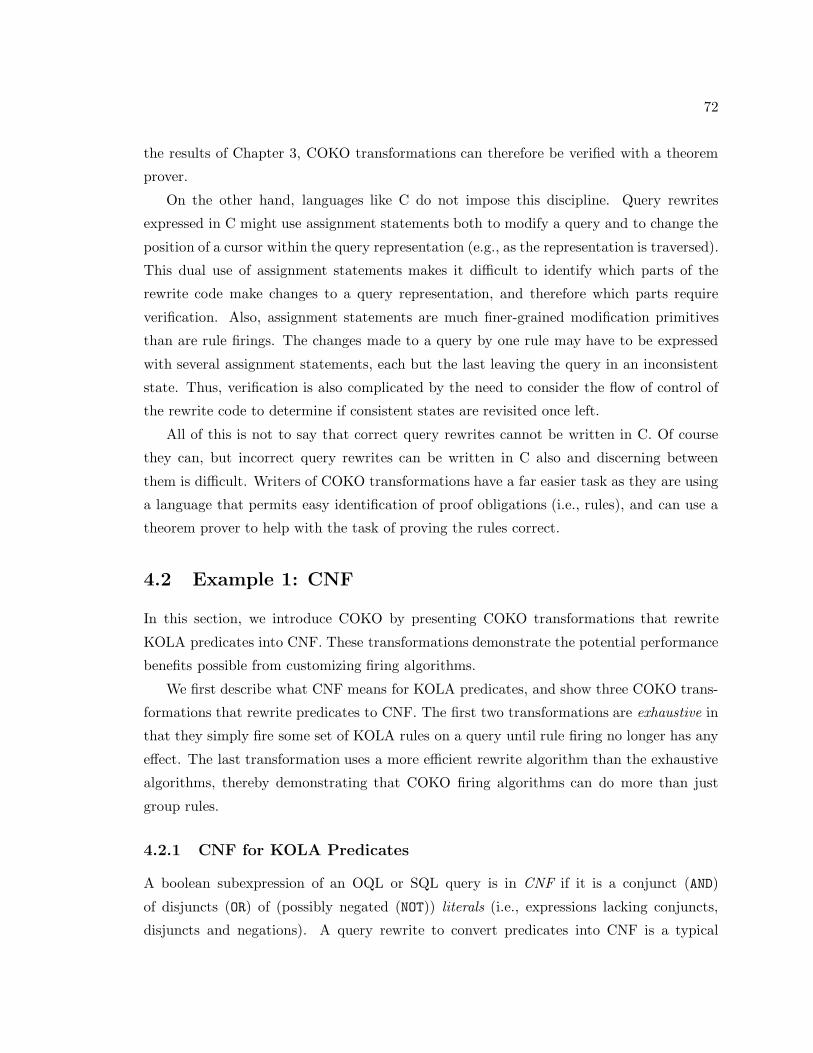
72
the results of Chapter 3, COKO transformations can therefore be verified with a theorem
prover.
On the other hand, languages like C do not impose this discipline. Query rewrites
expressed in C might use assignment statements both to modify a query and to change the
position of a cursor within the query representation (e.g., as the representation is traversed).
This dual use of assignment statements makes it difficult to identify which parts of the
rewrite code make changes to a query representation, and therefore which parts require
verification. Also, assignment statements are much finer-grained modification primitives
than are rule firings. The changes made to a query by one rule may have to be expressed
with several assignment statements, each but the last leaving the query in an inconsistent
state. Thus, verification is also complicated by the need to consider the flow of control of
the rewrite code to determine if consistent states are revisited once left.
All of this is not to say that correct query rewrites cannot be written in C. Of course
they can, but incorrect query rewrites can be written in C also and discerning between
them is difficult. Writers of COKO transformations have a far easier task as they are using
a language that permits easy identification of proof obligations (i.e., rules), and can use a
theorem prover to help with the task of proving the rules correct.
4.2 Example 1: CNF
In this section, we introduce COKO by presenting COKO transformations that rewrite
KOLA predicates into CNF. These transformations demonstrate the potential performance
benefits possible from customizing firing algorithms.
We first describe what CNF means for KOLA predicates, and show three COKO trans-
formations that rewrite predicates to CNF. The first two transformations are exhaustive in
that they simply fire some set of KOLA rules on a query until rule firing no longer has any
effect. The last transformation uses a more efficient rewrite algorithm than the exhaustive
algorithms, thereby demonstrating that COKO firing algorithms can do more than just
group rules.
4.2.1 CNF for KOLA Predicates
A boolean subexpression of an OQL or SQL query is in CNF if it is a conjunct (AND)
of disjuncts (OR) of (possibly negated (NOT)) literals (i.e., expressions lacking conjuncts,
disjuncts and negations). A query rewrite to convert predicates into CNF is a typical

73
preprocessing step in the course of rewriting. For example, this rewrite might be fired
before selection predicates are reordered.
A KOLA predicate p is in CNF if for any argument x, p ? x reduces by the definitions
of Tables 3.1, 3.2, and 3.3 to a boolean expression that is in CNF. Put another way, p is
in CNF if it is a conjunction (&) of disjunctions (|) of (possibly negated (∼)) literals (i.e.,
predicates lacking subpredicates of forms, (q & r), (q | r) or (∼ (q))).
Figures 4.1a and 4.1b shows example KOLA predicates over the Thomas schema of
Table 2.1. Both queries contain subpredicates (literals) over pairs of committees ([x, y])
• Pk: which when invoked on a pair, [x, y] is equivalent to the OQL expresssion,
x.chair.pty == y.chair.pty,
• Qk: which when invoked on a pair, [x, y] is equivalent to the OQL expresssion,
x.chair.terms > y.chair.terms,
• Rk: which when invoked on a pair, [x, y] is equivalent to the OQL expresssion,
x.topic == ‘‘NSF’’, and
• Sk: which when invoked on a pair, [x, y] is equivalent to the OQL expresssion,
(x.chair.terms + SUM
(SELECT y.terms
FROM y IN x.mems
)) > 100
The query of Figure 4.1b is equivalent to that of Figure 4.1a, but is in CNF.
4.2.2 An Exhaustive Firing Algorithm
Figure 4.2 shows two COKO transformations that convert KOLA predicates lacking nega-
tions (i.e., subpredicates of the form, ∼ (p)) into CNF. A COKO transformation begins
with the keyword, TRANSFORMATION, followed by the name of the transformation. The rest
of the transformation consists of two parts:
• a rule section (introduced by the keyword, USES) that lists the KOLA rewrite rules
and other COKO transformations fired by the transformation, and
• a firing algorithm (delimited by keywords BEGIN and END).

74
(Pk & Qk & Rk) | Sk (Pk | Sk) & (Qk | Sk) & (Rk | Sk)(a) (b)
such that
Pk = eq ⊕ 〈f ◦ π1, f ◦ π2〉,Qk = gt ⊕ 〈g ◦ π1, g ◦ π2〉,Rk = eq ⊕ 〈topic ◦ π1, Kf (‘‘NSF’’)〉,Sk = gt ⊕ 〈add ◦ 〈g ◦ π1, sum ◦ h ◦ mems ◦ π1〉, Kf (100)〉
f = pty ◦ chairg = terms ◦ chairh = iterate (Kp (true), terms)
Figure 4.1: A KOLA Predicate Before (a) and After (b) its Transformable into CNF
TRANSFORMATION CNF-BUUSES
d1: (p & q) | r →= (p | r) & (q | r)d2: r | (p & q) →= (p | r) & (q | r)
BEGINBU {d1 || d2} → CNF-BU
END
TRANSFORMATION CNF-TDUSES
d1: (p & q) | r →= (p | r) & (q | r)d2: r | (p & q) →= (p | r) & (q | r)
BEGINTD {d1 || d2} → CNF-TD
END
(a) (b)
Figure 4.2: Exhaustive CNF Transformations Expressed in COKO
A COKO transformation can be fired on any KOLA parse tree (example KOLA parse
trees are shown in Figure 4.3), and may transform this tree as a result. In describing the
transformations of Figure 4.4, we will assume that they have been fired on the parse tree
for some KOLA predicate p. Hereafter, we will use p to name the KOLA predicate and its
parse tree and rely on context to differentiate between the two.
CNF-BU
CNF-BU uses two KOLA rewrite rules that distribute disjunctions over conjunctions:
d1 : (p & q) | r →= (p | r) & (q | r)d2 : r | (p & q) →= (p | r) & (q | r)

75
1
2 3
4
6
7
5
21
(a) (b)
Fires d1
Pk
&
|
&
&
| |
&
Fires d1
Qk Rk
Sk
Pk Sk Sk
Qk Rk
3
4 5
6 7
8
9
21
(c)
&
& &
| |Sk
Sk Sk
Pk
Qk Rk
3
4 5
6
7 8
9
10
11
Figure 4.3: Illustrating CNF-BU on the KOLA Predicate of Figure 4.1a
In relation to a KOLA parse tree, the effect of either rule is to “push down” a disjunction
(|) past a conjunction (&). Fired exhaustively on an unnegated predicate, these rules “push
down” all disjuncts past all conjuncts, thereby leaving the predicate in CNF.
The firing algorithm for CNF-BU consists of the single complex COKO statement,
BU {d1 || d2} → CNF-BU.
This statement can be broken down as follows:
• d1 and d2 are rule firing statements. That is, by referencing these rules in the firing
algorithm (and provided each was defined in the rule section), these rules get fired.
Each rule succeeds in firing if, as a result of pattern matching, its head pattern matches
with the KOLA predicate on which it is fired.
• BU {d1 || d2} instructs the transformation to perform a bottom-up (or more accurately,
a preorder) traversal of predicate p, executing the statement,
{d1 || d2}
on each visited subtree, s. The effect of executing this statement on s is to first fire
d1 on s. If d1 succeeds in firing, then the statement is finished executing. If d1 fails
to fire, then d2 is fired on s. This statement succeeds if either d1 or d2 successfully
fires, and fails if both rules fail. The full statement
BU {d1 || d2}
succeeds if the statement,
{d1 || d2}

76
succeeds when executed on any subtree. Therefore, the effect of this statement as a
whole is to perform a bottom-up pass of p, firing d1 and d2 on each visited subtree
and succeeding if one of these rules successfully fires once.
• BU {d1 || d2} → CNF-BU executes the statement,
BU {d1 || d2},
and if it succeeds, fires CNF-BU recursively. Therefore, the effect of this statement (and
the transformation as a whole) is to perform successive bottom-up passes of p, firing
rules d1 and d2, and continuing with new passes until a pass of p is completed where
no rules have successfully fired. Put another way, this transformation fires rules d1
and d2 exhaustively in bottom-up fashion.
Figure 4.3 illustrates the effect of firing CNF-BU on the KOLA predicate of Figure 4.1a.
Figure 4.3a shows the parse tree representation of this predicate before it is transformed.
The bottom-up pass visits the subtrees rooted at shaded nodes of the initial tree in the
order indicated beneath each. Attempts to fire d1 and d2 on each proper subtree fail. But
d1 successfully fires on the root, resulting in the predicate tree of Figure 4.3b. Because
d1 successfully fired, another bottom-up pass is initiated on the tree resulting from firing
(Figure 4.3b). Rule d1 fires successfully on the 8th subtree visited during this pass, resulting
in the parse tree of Figure 4.3c. A final pass is performed over this parse tree where no
rules successfully fire. Therefore, the tree of Figure 4.3c is returned as the final result of
the transformation.
CNF-TD
Transformation CNF-TD (Figure 4.2b) is also an exhaustive algorithm for CNF. Unlike
CNF-BU, CNF-TD fires rules in top-down (i.e., inorder) fashion during each pass, as indi-
cated by the COKO operator TD. For CNF, the order in which subtrees are visited makes
no difference to the final result. Rules d1 and d2 form a confluent set — the same result
is returned no matter what order these rules are fired and no matter in what order parse
trees are visited, provided that these rules are fired exhaustively.
Though the order in which subtrees are visited during rule firing has no effect on the
predicate that results, order does affect the performance of the query rewrite itself. Table 4.1
shows a performance comparison of CNF-TD and CNF-BU. The transformations were compiled
with our COKO compiler (described in Section 4.3.3) into C++ code which in turn was
compiled on Sparcstation 10’s using the Sun C++ compiler. For each height class, both

77
Height Elapsed CPUCNF-TD CNF-BU CNF-TD CNF-BU
4 0.17 0.17 0.07 0.075 0.42 0.48 0.23 0.266 1.19 2.05 1.07 1.687 3.24 4.18 3.05 3.988 7.71 12.95 6.69 11.63
Table 4.1: Average Times (in seconds) for CNF-TD and CNF-BU
transformations were run on the same 25 randomly generated queries. Both the elapsed
time (the total time taken by the system to perform the rewrite) and the CPU time (the
time for which the CPU is busy) were measured, and the times for all 25 queries were
averaged.
For CNF, top-down exhaustive firing has better performance overall than bottom-up
exhaustive firing. The performance discrepancy is due to the rules involved in these trans-
formations. Consider that the result of firing either rule successfully is a conjunction of
the form, (p | r) & (q | r). If additional rule firings are required, it would be because p
(Case 1), q (Case 2) or r (Case 3) are of the form p1 & p2, or because (Case 4) the entire
predicate is a subpredicate, p1 of some disjunctive predicate, p1 | p2. Each of the four cases
is equally likely given that our randomized query generating algorithm decides that a node
is a conjunct or disjunct with equal probability. But top-down passes of the query tree will
“catch” cases 1, 2 or 3 on the same pass that resulted in the initial firing because p, q and
r will be subtrees of the newly formed predicate. On the other hand, a bottom-up pass
will only “catch” case 4 on the same pass as the initial firing, and will require an additional
pass to “catch” cases 1, 2 and 3. Therefore, a bottom-up transformation is more likely to
require an additional pass to deal with the repercussions of a successful rule firing. This
example illustrates how even subtle differences in firing algorithms such as traversal order
can result in differences in performance. As we show below, the performance differences
become marked when exhaustive firing algorithms can be avoided altogether.
4.2.3 A Non-Exhaustive Firing Algorithm for CNF
Figure 4.4 shows an alternative COKO transformation (CNF) that rewrites KOLA predicates
into CNF using a firing algorithm that is more efficient than the exhaustive algorithms of
CNF-BU and CNF-TD. When CNF is fired on a predicate p, the statement
BU CNFAux

78
TRANSFORMATION CNFUSESCNFAux
BEGINBU CNFAux
END
TRANSFORMATION CNFAuxUSES
d1: (p & q) | r →= (p | r) & (q | r)d2: r | (p & q) →= (p | r) & (q | r)
BEGIN{d1 || d2} →
{GIVEN p′ & q′ DO {CNFAux (p′); CNFAux (q′)}}END
(a) (b)
Figure 4.4: An Efficient CNF Transformation
performs a bottom-up pass of p, firing the auxiliary transformation, CNFAux on every subtree
of p. The effect of firing CNFAux on a subtree s is described below:
1. As in CNF-BU and CNF-TD, {d1 || d2} fires d1 on s, and then fires d2 on s if d1 fails.
2. Successful firing of either d1 or d2 results in the execution of the statement,
{GIVEN p′ & q′ DO {CNFAux(p′); CNFAux(q′)}}
on the predicate resulting from firing. This predicate will have the form,
(p | r) & (q | r).
The pattern, (p′ & q′) that follows the keyword GIVEN is matched with this predi-
cate (i.e., p′ gets bound to (p | r) and q′ gets bound to (q | r)) and CNFAux is fired
recursively on the subtrees bound to p′ and q′ respectively.
In short, CNF performs a bottom-up (BU) pass of p, firing the auxiliary transformation,
CNFAux, on each visited subtree. CNFAux fires rewrite rules d1 and d2 and if either succeeds,
initiates top-down passes on the conjunct subtrees that result from rule firing (by recursively
firing CNFAux). Each top-down pass proceeds until a subtree is visited on which both d1
and d2 fail to fire.
The effect of this transformation on the KOLA predicate of Figure 4.1a are illustrated
in Figure 4.5. Figure 4.5a shows the parse tree representation of this predicate before it is
transformed. The bottom-up pass visits the shaded nodes of the initial tree in the order
indicated beneath each. The firing of CNFAux fires d1 and d2. CNFAux fails to fire both
rules (and therefore fails to fire) on every visited subtree except the root which is visited

79
1
2 3
4
6
7
5 21
(a) (b)
Fires d1
Pk
&
|
&
&
| |
&
Fires d1
Qk Rk
Sk
Pk Sk Sk
Qk Rk
21
(c)
&
& &
| |Sk
Sk Sk
Pk
Qk Rk
Figure 4.5: Illustrating the CNF Firing Algorithm on the KOLA Predicate of Figure 4.1a
Height Elapsed CPUCNF-TD CNF CNF-TD CNF
4 0.17 0.15 0.07 0.055 0.42 0.20 0.23 0.106 1.19 0.35 1.07 0.247 3.24 0.59 3.05 0.488 7.71 1.35 6.69 1.17
Table 4.2: Average Times (in seconds) for CNF-TD and CNF
last (node 7). Firing d1 on the root results in the predicate tree of Figure 4.5b. Because
d1 successfully fired, CNFAux is fired recursively on the two disjuncts produced from firing
(the subtrees rooted by the shaded nodes of Figure 4.5b). Firing d1 and d2 on the first
of these subtrees fails, and therefore terminates the top-down pass of this subtree. But d1
fires successfully on the second subtree, producing the predicate tree of Figure 4.5c. Again,
successful firing initiates recursive firings of CNFAux on the subtrees rooted by the shaded
nodes of Figure 4.5c. d1 and d2 fail to fire on both subtrees, and the tree of Figure 4.5c is
returned.
Table 4.2 shows a performance comparison of the more efficient of the two exhaustive
CNF transformations (CNF-TD) and CNF. CNF was run on the same 25 randomly generated
queries as was used for the comparisons of Table 4.1. As before, both the elapsed time (the
total time taken by the system to perform the transformation) and the CPU time (the time
for which the CPU is busy) were measured, and the times for all 25 queries were averaged.
CNF exhibits far better performance than either of the exhaustive transformations. (For
predicates of height 8, performance was improved by a factor of 6.) Intuitively, this is

80
because CNF is discriminating in how it fires rules:
• Successful firing of either d1 and d2 requires both exhaustive transformations to per-
form additional passes over the entire query tree. On the other hand, successful firing
of either rule requires CNF to perform passes over only selected parts of the query tree.
• The exhaustive transformations require a complete pass of failed rule firings in order
to terminate. This pass is not required by transformation CNF.
The savings in rule firings is illustrated by considering how all three transformations
transform the KOLA predicate,
(Pk & Qk & Rk) | Sk.
CNF performs one complete and two partial passes over this predicate’s representation,
firing rules 20 times with two firings succeeding. On the other hand, CNF-TD performs
two complete passes over this predicate’s representation, firing rules 42 times with two
succeeding. CNF-TD performs three complete passes over this predicate’s representation,
firing rules 52 times with two succeeding.3
Exhibited Features of COKO Firing Algorithms
CNF exhibits the fine-grained control of rule and transformation firing supported by COKO
firing algorithms. It is this control that makes it possible to express efficient query rewrites.
COKO supports four forms of rule-firing control:
• Explicit Firing: Rewrite rules used within a transformation are named (e.g., d1 and
d2) and explicitly fired by the firing algorithm.
• Traversal Control: Both bottom-up (in CNF) and top-down (in CNFAux) passes can be
performed in the course of rewriting predicates into CNF.
• Selective firing: CNFAux is fired recursively on the two disjuncts that result from
successful firings of either d1 or d2. CNFAux is not fired on the conjunct resulting from
these firings because both d1 and d2 can only succeed on trees rooted by “|”.3For simplicity, we count each rule’s firing on a literal (such as Pk) as one firing. In fact, each literalis a subtree with multiple nodes. Therefore, visiting a literal results in more than one firing. Theseuncounted firings are the same for each algorithm. However, CNF will visit literals less frequently thanthe exhaustive transformations, and therefore will exhibit even better performance in comparison.

81
• Conditional firing: Some firings are conditioned on the success or failure of previous
firings. E.g., CNFAux fires d2 only if d1 fails; CNFAux is only fired recursively if one of
the rules d1 or d2 succeeds.
Correctness of CNF
Theorem 4.2.1 (Correctness) CNF is correct.
Proof: All query modification performed by CNF occurs as result of firing CNFAux, which in
turn occurs as result of firing rules d1 and d2. Therefore, CNF is correct if both rewrite rules
are correct. Rules d1 and d2 are proved correct by execution of the theorem prover scripts
of Appendix B.1 using LP [46]. �
Proof that CNF transforms all KOLA predicates into CNF follows below.
Lemma 4.2.1 Let p be a KOLA predicate tree lacking negations, and whose child subtrees
are in CNF. Then CNFAux (p) is in CNF.
Proof: (By induction on the height, h(p) of the highest &-node in p.) For the base case
(h(p) = 0) p must contain no &-nodes and therefore is in CNF and is returned untouched
by CNFAux. For the inductive case, either p is already in CNF and is returned untouched,
or p is not in CNF and is a disjunction, Q | R such that Q and R are in CNF and at least
one of Q or R is a conjunction (x0 & x1). For the case where exactly one of Q and R is
a conjunction, assume without loss of generality that Q is a conjunction. Then, h(Q) is
larger than both h(x0) and h(x1) because both x0 and x1 are children of a &-node. Further,
because R is in CNF it has no &-nodes and therefore h(p) = h(Q). Firing d1 on (Q | R)
returns (S & T ) such that S = (x0 | R) and T = (x1 | R), and CNFAux is subsequently fired
on S and T . But h(S) = h(x0) and h(T ) = h(x1) and therefore by induction, these firings
result in trees that are in CNF. Therefore, the tree returned by CNFAux (p) is in CNF.
For the case where both Q (x0 & x1) and R (y0 & y1) are conjunctions, h(p) is larger
than h(x0), h(x1), h(y0) and h(y0) as all of the latter subtrees are children of &-nodes.
Firing CNFAux on p fires d1 once, and d2 on each of the resulting disjuncts, leaving
(S1 & S2) & (T1 & T2)
such that S1 = (x0 | y0), S2 = (x1 | y0), T1 = (x0 | y1) and T2 = (x0 | y1). CNFAux is fired
on each of S1, S2, T1 and T2 and by induction, each of these firings return a predicate in
CNF. Therefore, CNFAux (p) is in CNF. �

82
TRANSFORMATION CNF-NEGUSESCNF,
involution: ∼ (∼ (p)) →= p,
deMorgan1: ∼ (p & q) →= ∼ (p) | ∼ (q),deMorgan2: ∼ (p | q) →= ∼ (p) & ∼ (q)BEGINTD {involution || deMorgan1 || deMorgan2};BU {involution};CNFEND
Figure 4.6: The Full CNF Transformation Expressed in COKO
Theorem 4.2.2 Let p be any KOLA predicate lacking negations. Then CNF (p) is in CNF.
Proof: Note that CNF (p) fires CNFAux on every subtree visited during a bottom-up traversal
of p. By Lemma 4.2.1, each firing leaves a subtree in CNF, and therefore p is left in
CNF. �
Accounting for Negations
Figure 4.6 contains a COKO transformation that transforms all KOLA predicates into CNF,
including those with negations. Besides using CNF, this transformation includes three other
rules:
• involution eliminates double negations,
• deMorgan1 pushes down a negation past a conjunction, and
• deMorgan2 pushes down a negation past a disjunction.
The firing algorithm for the full CNF transformation executes two statements on the
argument tree, p before firing CNF. These statements effectively push negations to the bot-
tom of p’s query tree while ensuring that consecutive negations are eliminated. The first
statement performs a top-down pass of p firing the involution and deMorgan rules on each
subtree visited during the traversal. Involution is then performed in a bottom-up pass of
the resulting tree. This second pass is necessary because the first pass may construct doubly
negated predicates. For example, a predicate of the form,
∼ (∼ (p) & q)

83
will be transformed after the first pass to
∼ (∼ (p)) | ∼ (q)
which must be transformed by a second pass firing the involution rule to
p | ∼ (q).
Once all negations have been pushed to the bottom of the query (i.e., below all conjuncts and
disjuncts), the resulting predicate can then be transformed into CNF using transformation
CNF.
We have introduced COKO with a simple yet practical example. The normalization of
predicates into CNF is a typical preprocessing rewrite for useful rewrites such as one that
reorders selection predicates. We showed a COKO transformation (CNF) that performs this
rewrite for predicates lacking negations and a complete COKO transformation (CNF-NEG)
that removes this restriction and fires CNF as if it were a subroutine. Because its rules are
confluent, CNF can also be implemented with exhaustive firing algorithms as in CNF-BU
and CNF-TD. But exhaustive firing is an inefficient means of performing this transforma-
tion. Therefore, this example demonstrates the potential performance benefits from using
customized firing algorithms to express complex query rewrites.
4.3 The Language of COKO Firing Algorithms
The semantics of statements that appear in COKO transformation firing algorithms have
two parts:
• their operation (what they do when executed), and
• their success value (what they return as a result of execution).
Success values are truth values that indicate if a statement succeeds when executed. For
example, fired rules return success values of true if their head patterns match the expressions
on which they are fired. In general, success values are intended to indicate whether or not
a statement accomplishes what it is intended to do. Note that a success value of false does
not, in general, mean that a statement has failed to modify the expression on which it was
executed.

84
4.3.1 The COKO Language
Below we present COKO’s statements, categorizing them by the kinds of firing control they
provide. Each is presented with its operation and success value semantics. For the purposes
of discussion, we assume that statements are contained in some transformation that has
been fired on some KOLA query tree, p.
Explicit Firing
Rules and transformations declared in the USES section of a transformation can be fired as if
they were procedures invoked in a programming language such as C. Rules and transforma-
tions can be fired on subtrees of p named by pattern variables (see Section 4.3.1) or can be
fired on p directly, in which case no argument needs to be named. As well, rules that use the
same pattern variables in their heads and their bodies can be fired inversely. For example,
d1 of Figure 4.4 could be fired inversely (d1 INV) to factor a common subexpression (r)
from a conjunction of disjuncts. Rule (and inverse rule) firings return true as their success
values if they successfully fire. Transformation firings succeed if the complex statements
that are their main bodies succeed (see Section 4.3.1).
Traversal Control
Query trees can be traversed in bottom-up (postorder) or top-down (preorder) fashion. For
any statement S,
BU S
performs a bottom-up pass of p executing S on every subtree. Analagously, TD S executes
S on every subtree during a top-down pass of p. Both traversal statements return a success
value of true if S succeeds when fired on some subtree visited during the traversal. Also,
REPEAT S
fires S repeatedly on p until S no longer succeeds, and returns a success value of true if
S succeeds at least once. Thus far, we have found BU, TD and REPEAT to be sufficient for
expressing the kinds of traversal control we have needed to express for our firing algorithms.
Our COKO compiler could be easily extended however, should we determine the need for
another form of traversal control at a later point.

85
Selective Firing
Rules and transformations need not be fired on all of p and can instead be fired on selected
subtrees of p. These subtrees are identified by matching patterns to query trees using
COKO’s GIVEN statement.
GIVEN patterns are like rule patterns, but can also include “don’t care” variables (“ ”),4
which act like pattern variables, but whose bindings are ignored. The COKO matching
statement, GIVEN, identifies these patterns with variables, producing environments for use
in subsequent statements. A GIVEN statement has the form,
GIVEN eqn1, . . ., eqnn DO S.
such that S is any COKO statement, and each “equation”, eqni is of the form,
<variablei > = <patterni >
(or just patterni, if this pattern is to be matched with all of p). The processing of eqni results
in an attempted match of patterni with the tree previously bound to variablei. Successful
matching adds the variables appearing in patterni (and the subtrees that they matched) to
an environment that is then visible to equations appearing after eqni and S. The success
value for the entire GIVEN statement is true if all n equations successfully match.
Unlike most programming languages, the environment visible inside statement S can
shrink dynamically. Dynamically varying environments are necessary because environment
entries label parts of a tree that can become obsolete as a result of a rule or transformation
firing. To illustrate, suppose that the GIVEN statement,
GIVEN f ! , f = g ◦ , g = 〈h, π2〉 DO {transform-1 (g); transform-2 (h)}
were executed on the query,
(〈π1, π2〉 ◦ π1) ! [[x, y], z].
The result of matching the three equations is to create an environment consisting of the
labels f, g and h matched with the subtrees shown in Figure 4.7a.
Suppose that transform-1 is a transformation or rule that replaces g with a completely
new tree. For example, transform-1 could be the rule,
〈π1, π2〉 →= id.
4The COKO compiler recognizes four different “don’t care” variables denoting predicates ( P), functions( F), objects ( O) and Bools ( B) respectively. To simplify the presentation, we will use only a single“don’t care” variable ( ) for the examples presented in this thesis.

86
f −→
g −→
h −→
π1
[ ]
[ ]
x y
z
!
◦
id
π1
(b)π2
◦
〈 〉
π1 π2
π1
[ ]
[ ]
x y
z
!
f −→
g −→
h −→
(a)
Figure 4.7: The Effects of a GIVEN Statement on Environments
Then the result of this firing would invalidate all variable bindings to trees that were proper
subtrees of g (i.e., h), as these would no longer point to valid subtrees. Thus, the result of
this firing would be to change the environment seen by the statement that follows to remove
invalidated variable bindings, to the transformed environment of Figure 4.7b that no longer
includes an entry for h.
The COKO compiler performs a dependency analysis of variables declared in matching
equations, and indicates at compile time if a variable is used after it is invalidated. Thus,
it would flag the firing of transform-2 (h) in this example as an error. In general, the
invalidation of a variable, v occurs following execution of some statement S provided that
S is a statement that modifies a query (i.e., a firing of a rule or another transformation),
and S is executed on some variable w such that v names a subtree of the tree named by w.
Conditional Firing
One can condition the execution of a COKO statement, S ′ on the result of a previous
statement, S in three ways:
• S → S ′ executes S and then executes S ′ if S succeeds. This statement succeeds if S
succeeds.
• S || S ′ executes S and then executes S ′ if S fails. This statement succeeds if S or S ′
succeed.
• S ; S ′ executes S and then executes S ′. This statement succeeds if either S or S ′
succeed.

87
The complex statement connector,“→” is right-associative, and “|” and “;” are left-associative.
One can override default associativities using braces ({}).
4.3.2 TRUE, FALSE and SKIP
TRUE, FALSE and SKIP allow one to circumvent the default success values associated with
COKO statements. For any statement, S,
TRUE S
executes S and returns a success value of true, regardless of the success value of S. (Similarly,
FALSE S returns a success value of false.)
The statement SKIP performs no action at all and returns a success value of true. This
statement is useful if one wants to define a transformation that returns a success value of true
only if it rewrites expressions to a particular form. For example, consider a transformation
whose purpose is to rewrite KOLA functions into constant functions (i.e., of the form,
Kf (x) for some x). It might be desirable to return a success value of true only if functions
that result from the transformation are of this form. However, the firing algorithm for
this transformation may be a complex statement, S that does not always return the proper
success value. In this case, one can achieve the desired effect by replacing the firing algorithm
withFALSE S;
GIVEN Kf (x) DO SKIP
The effect of this firing algorithm is to first execute S. Then, if a constant function is
produced by S, the subsequent GIVEN statement succeeds and a success value of true is
returned (because the “;”-separated statement succeeds if either of the separated statements
succeeds, and because the GIVEN statement succeeds if the pattern, Kf (x) successfully
matches the expression resulting from executing S). If a constant function is not generated
by S, the GIVEN statement fails and so too does the transformation as a whole.
4.3.3 The COKO Compiler
We have implemented a compiler for COKO ([68]) that generates C++ classes from COKO
transformations. Objects of these generated classes manipulate KOLA trees according to
the firing algorithm of the compiled COKO transformation. The compiler has an object-
oriented design. Every COKO statement is implemented with its own C++ class. Each
of these classes is a subclass of the virtual class, Statement, and is obligated to define a

88
method exec that takes an environment of variable-to-KOLA tree bindings as input and
produces a transformed version of this environment as output. These environments include
entries for the trees on which each statement is executed.
The compilation of a COKO transformation generates a new subclass of Statement,
complete with an implementation of an exec method. The exec method definition for a
compiled transformation simply constructs a tree of COKO Statement objects correspond-
ing to the parse structure of the COKO code, and then invokes exec on the root. By
compiling COKO transformations into Statements, COKO’s language of firing algorithms
is made extensible even at the level of its implementation.
4.4 Example 2: “Separated Normal Form” (SNF)
In this section we describe a novel normalization and show its expression in COKO. The
normalization is of binary predicates, (in KOLA, predicates on pairs) and involves isolating
those subpredicates that act as unary predicates on just one argument. This normalization
is a useful preprocessing step when unary predicates need to be moved to other parts of
the query as in predicate-pushdown, join-reordering and magic-sets rewrites. Because this
normalization “separates” unary and binary subpredicates, we characterize the predicates
that result as being in “Separated Normal Form” or SNF.
The point of this example is to show that COKO transformations are expressive enough
to to be used in place of rules in existing rule-based systems. We make this point in several
ways:
• The SNF normalization is more complex than CNF, even firing CNF as part of its firing
algorithm. Therefore, COKO is expressive enough to capture complex normalizations.
• SNF is itself fired in the firing algorithms of many transformations that are not nor-
malizations. These include predicate-pushdown (Section 4.5.1), join-reordering (Sec-
tion 4.5.2) and Magic-Sets rewrites (Section 4.6). These examples show that COKO
can express a wide variety of complex rewrites in modular fashion.
• SNF is not usually thought of as a normalization, and as far as we know has not been
expressed before with declarative rewrite rules. Thus, COKO can express rewrites
that are usually expressed only with code.

89
4.4.1 Definitions
Intuitively, a KOLA binary predicate, op on pairs [x, y] is in SNF if it is of the form,
p & q & r
such that p is a unary predicate on x, q is a unary predicate on y and r is the minimal
subpredicate of op that is a predicate on both x and y. In this section, we present a
COKO transformation (SNF) that converts unnested SQL predicates into SNF. More formal
definitions follow.
Qualifications
A qualification predicate is defined by Ramakrishnan [80] as:
... a Boolean combination (i.e., an expression using the logical connectives AND,
OR and NOT) of conditions of the form expression cmp expression, where cmp is
one of the comparison operators {<, <=, =, <>, >=, >}, [and an] expression
is a column name, a constant or an arithmetic or string expression.
Essentially, qualifications are the predicates of unnested SQL queries.
KOLA qualification predicates are translations of SQL qualification predicates. They
are defined formally in terms of basic functions (the KOLA equivalents of expressions) and
basic predicates (the KOLA equivalents of conditions).
Definition 4.4.1 (Basic Functions) A basic function is a KOLA function of one of the
forms below:
• att ◦ π1 such that att is a primitive attribute (e.g., a column name),
• att ◦ π2 such that att is a primitive attribute,
• Kf (c) such that c is a constant, or
• op ◦ 〈f, g〉 such that f and g are basic functions and op is a binary primitive function
(e.g., add).
Definition 4.4.2 (Basic Predicate) A basic predicate is a predicate of the form,
p ⊕ 〈f , g〉
such that p is a binary primitive (eq, lt, gt, leq, geq or neq), and f and g are basic
functions.

90
Definition 4.4.3 (Qualifications) A KOLA qualification predicate is a predicate consist-
ing of conjunctions (&), disjunctions (|) and negations (∼) of basic predicates.
SNF
We begin by defining functions and predicates that are inherently binary. Intuitively, in-
herently binary functions and predicates cannot be simplified in any way that makes them
unary.
Definition 4.4.4 (Inherently Binary Functions) A KOLA function f is inherently bi-
nary if it is of either of the forms:
• op ◦ 〈f ◦ π1, g ◦ π2〉,
• op ◦ 〈f ◦ π2, g ◦ π1〉, or
• op ◦ 〈f, g〉 such that f or g is inherently binary.
Definition 4.4.5 (Inherently Binary Predicates) A KOLA predicate p is inherently
binary if it is of the form,
p ⊕ f
such that f is an inherently binary function, or of the form.
p | q
such that
• p or q is inherently binary, or
• one of p or q is of the form (r1 ⊕ π1) and the other is of the form (r2 ⊕ π2).
Definition 4.4.6 (SNF) A KOLA predicate p is in SNF if it is of the form,
(ρ ⊕ π1) & (σ ⊕ π2) & τ
such that τ is a conjunction,
τ1 & . . . & τm
of inherently binary and constant (Kp (b)) predicates.

91
(ρ ⊕ π1) & (σ ⊕ π2) & τ such that
ρ = (R2k | S2k)σ = Kp (true)τ = ((Pk | (S2k ⊕ π1)) & (Qk | (S2k ⊕ π1)))
Pk = eq ⊕ 〈f ◦ π1, f ◦ π2〉,Qk = gt ⊕ 〈g ◦ π1, g ◦ π2〉,R2k = eq ⊕ (〈id, Kf (‘‘NSF’’)〉 ◦ topic)S2k = gt ⊕ (〈id, Kf (100)〉 ◦ (add ◦ 〈g, sum ◦ h ◦ mems〉))
f = pty ◦ chairg = terms ◦ chairh = iterate (Kp (true), terms)
Figure 4.8: The SQL/KOLA Predicates of Figure 4.1 in SNF
Given any pair argument [x, y], (ρk ⊕ π1) ? [x, y] = ρk ? x and therefore ρk denotes
a predicate that requires only the first of its arguments. Similarly, σk denotes a predicate
requiring the second argument. The restriction that τ consist of inherently binary predicates
ensures that a predicate in SNF has “moved” as many non-constant subpredicates into ρ
and σ as possible. Figure 4.8 shows the SNF equivalent of the KOLA predicates of Figure
4.1. Note that for this predicate, τ is a conjunction of inherently binary predicates,
Pk | (S2k ⊕ π1)
(which is inherently binary because Pk is inherently binary), and
Qk | (S2k ⊕ π1)
(which is inherently binary because Qk is inherently binary).
4.4.2 A COKO Transformation for SNF
A COKO transformation that rewrites qualification predicates into SNF is shown in Fig-
ure 4.9 and its auxiliary transformations are shown in Figure 4.10. The latter figure contains
three COKO transformations: SimpLits, LBConj and OrderConjs.
Tracing the Execution
The firing algorithm for transformation SNF of Figure 4.9 consists of the seven steps de-
scribed below. We demonstrate these steps by showing how this transformation rewrites

92
TRANSFORMATION SNFUSESSimpLits, CNF, LBConj, OrderConjs,
init : p→= (Kp (true) ⊕ π1) & (Kp (true) ⊕ π2) & Kp (true) & p,
pull1 : (p ⊕ f) | (q ⊕ f) →= (p | q) ⊕ f,
pull2 : (p ⊕ f) | Kp (b) →= (p | Kp (b)) ⊕ f,
pull3 : Kp (b) | (q ⊕ f) →= (Kp (b) | q) ⊕ f,
pull4 : Kp (b1) | Kp (b2) →= Kp (b1 OR b2),simp : Kp (true) & p
→= pBEGINSimpLits; -- (1)CNF; -- (2)init; -- (3)BU {pull1 || pull2 || pull3 || pull4}; -- (4)LBConj; -- (5)OrderConjs; -- (6)GIVEN (p ⊕ π1) & (q ⊕ π2) & r DO {simp (p); simp (q); simp (r)} -- (7)
END
Figure 4.9: The SNF Normalization Expressed in COKO
qualification predicate p of Figure 4.1a:
Pk = eq ⊕ 〈f ◦ π1, f ◦ π2〉,Qk = gt ⊕ 〈g ◦ π1, g ◦ π2〉,Rk = eq ⊕ 〈topic ◦ π1, Kf (‘‘NSF’’)〉,Sk = gt ⊕ 〈add ◦ 〈g ◦ π1, sum ◦ h ◦ mems ◦ π1〉, Kf (100)〉
f = pty ◦ chair
g = terms ◦ chair
h = iterate (Kp (true), terms)
into the predicate of Figure 4.8. Figures 4.11 and 4.12 show the parse tree for this predicate
at various stages during the execution of the transformation. The original predicate tree is
shown in Figure 4.11a.
Step 1: The first step of SNF fires the transformation SimpLits (Simplify Literals) shown
in Figure 4.10. The effect of firing SimpLits is to reduce subpredicates of the form (p ⊕ f)
to the forms (p ⊕ π1) or (p ⊕ π2) if such a reduction is possible. More precisely, SimpLits

93
TRANSFORMATION SimpLitsUSES
sft : f ◦ (g ◦ h) →= (f ◦ g) ◦ h
sl1 : 〈Kf (x), Kf (y)〉 →= Kf ([x, y]),sl2 : f ◦ Kf (x) →= Kf (f ! x),sl3 : 〈f, Kf (x)〉 →= 〈id, Kf (x)〉 ◦ f,
sl4 : 〈Kf (x), f〉 →= 〈Kf (x), id〉 ◦ f,
sl5 : 〈f ◦ h, g ◦ h〉 →= 〈f, g〉 ◦ h,
sl6 : p ⊕ (f ◦ g) →= p ⊕ f ⊕ g,
sl7 : p ⊕ Kf (x) →= Kp (p ? x)BEGINBU {sl1 || sl2 || {{sl3 || sl4} → REPEAT sft} || sl5 || sl6 || sl7 || REPEAT sft}END
TRANSFORMATION LBConjUSESsftp : p & (q & r) −→ (p & q) & rBEGINBU {sftp → {GIVEN p & DO LBConj (p)}}END
TRANSFORMATION OrderConjsUSES
oc1 : (p ⊕ π1) & (q ⊕ π2) & r & (s ⊕ π1)→= ((p & s) ⊕ π1) & (q ⊕ π2) & r,
oc2 : (p ⊕ π1) & (q ⊕ π2) & r & (s ⊕ π2)→= (p ⊕ π1) & ((q & s) ⊕ π2) & r,
oc3 : (p ⊕ π1) & (q ⊕ π2) & r & s→= (p ⊕ π1) & (q ⊕ π2) & (r & s)
BEGINBU {oc1 || oc2 || oc3}END
Figure 4.10: Auxiliary Transformations Used by SNF

94
transforms any basic predicate lacking subfunctions of the form (f ◦ π1) to either of the
forms (p ⊕ π2) or Kp (x) (and similarly for predicates lacking (f ◦ π2) as a subfunction).
SimpLits performs a single bottom-up pass of the input predicate, firing rules
sl1, . . . , sl7
on each visited subtree. Rules sl1, . . . , sl5 only fire successfully on function subtrees while
sl6 and sl7 only fire successfully on predicate subtrees. Because the pass is bottom-up, a
basic predicate is visited only after its subfunctions are visited.
SimpLits rewrites Rk (to R2k) and Sk (to S2k) but has no effect on Pk or Qk. In rewriting
Rk, SimpLits first fires rule sl3 on its subfunction,
〈topic ◦ π1, Kf (‘‘NSF’’)〉
generating
〈id, Kf (‘‘NSF’’)〉 ◦ (topic ◦ π1).
The successful firing of sl3 triggers the firing of sft leaving
(〈id, Kf (‘‘NSF’’)〉 ◦ topic) ◦ π1.
Finally, rule sl6 fires on the entire predicate leaving (R2k ⊕ π1).
When fired on Sk, SimpLits first fires sl5 on its subfunction
〈g ◦ π1, sum ◦ h ◦ mems ◦ π1〉
leaving
〈g, sum ◦ h ◦ mems〉 ◦ π1.
Then, sl3, sft and sl6 fire, resulting in (S2k ⊕ π1). Therefore, the result of firing SimpLits
on p is
p1 = (Pk & Qk & (R2k ⊕ π1)) | (S2k ⊕ π1)
as illustrated in Figure 4.11b.
Step 2: Next, transformation CNF of Figure 4.4 is fired. Applied to p1, this firing results
in
p2 = (Pk | (S2k ⊕ π1)) & (Qk | (S2k ⊕ π1)) & ((R2k ⊕ π1) | (S2k ⊕ π1))
as illustrated in Figure 4.11c.

95
Step 3: Rule init is fired, appending trivial conjuncts to the current predicate. The
purpose of this step is to ensure the satisfaction of an invariant for Step 4 which performs
a bottom-up pass on the resulting predicate. This invariant establishes that every subtree
visited during this bottom-up pass is of the form,
(ρ ⊕ π1) & (σ ⊕ π2) & τ
such that τ is a conjunction of subpredicates to be “appended” to either ρ, σ or neither.
Fired on p2, this step results in
p3 = (Kp (true) ⊕ π1) & (Kp (true) ⊕ π2) & Kp (true) & p2
as illustrated in Figure 4.11d.
Step 4: This step executes the COKO statement,
BU {pull1 || pull2 || pull3 || pull4}.
The effect of firing these rules in bottom-up fashion is to “pull” common functions out of
disjuncts. For example, the result of executing pull1 on p3’s subpredicate,
(R2k ⊕ π1) | (S2k ⊕ π1)
is (R2k | S2k) ⊕ π1. Therefore, this step converts disjuncts to the forms (p ⊕ π1) or
(p ⊕ π2) where possible. Applied to p3, this statement results in
p4 =((Kp (true) ⊕ π1) & (Kp (true) ⊕ π2) & Kp (true)) &
((Pk | (S2k ⊕ π1)) & (Qk | (S2k ⊕ π1)) & ((R2k | S2k) ⊕ π1)
as illustrated in Figure 4.11e.
Step 5: This step executes the COKO transformation, LBComp. This transformation
rewrites a predicate that is in CNF,
p1 & p2 & . . . & pn
(with conjunctions associated in any way), into a predicate of the form,
(. . . (p1 & p2) & . . . & pn)
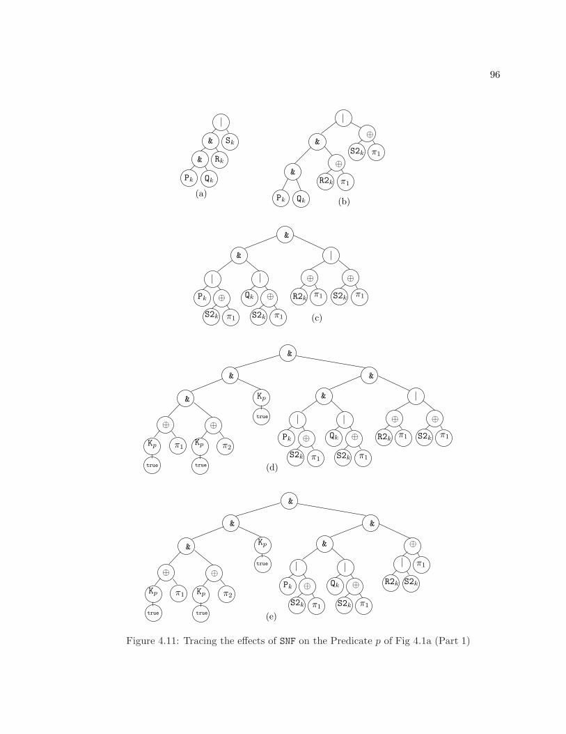
96
(a)(b)
Pk
|&
&
Sk
Rk
Qk
⊕π1S2k
⊕π1R2k
|
&
&
Pk Qk
(c)
Pk
|&
S2kR2kQk
&
| | ⊕ ⊕⊕ ⊕
π1 π1
π1 π1
S2k S2k
Kp
(d)
&
&
&
Pk
|⊕
π1S2k
Qk
|⊕
π1S2k
|
R2k
⊕π1 S2k
⊕π1
&
Kp
true
&
⊕
π2
true
⊕
π1Kp
true
(e)
&
&
&
⊕Kp
true
π1
⊕Kp
true
π2
Kp
true
&
&
Pk
|⊕
π1S2k
Qk
|⊕
π1S2k
|R2k
⊕
S2k
π1
Figure 4.11: Tracing the effects of SNF on the Predicate p of Fig 4.1a (Part 1)
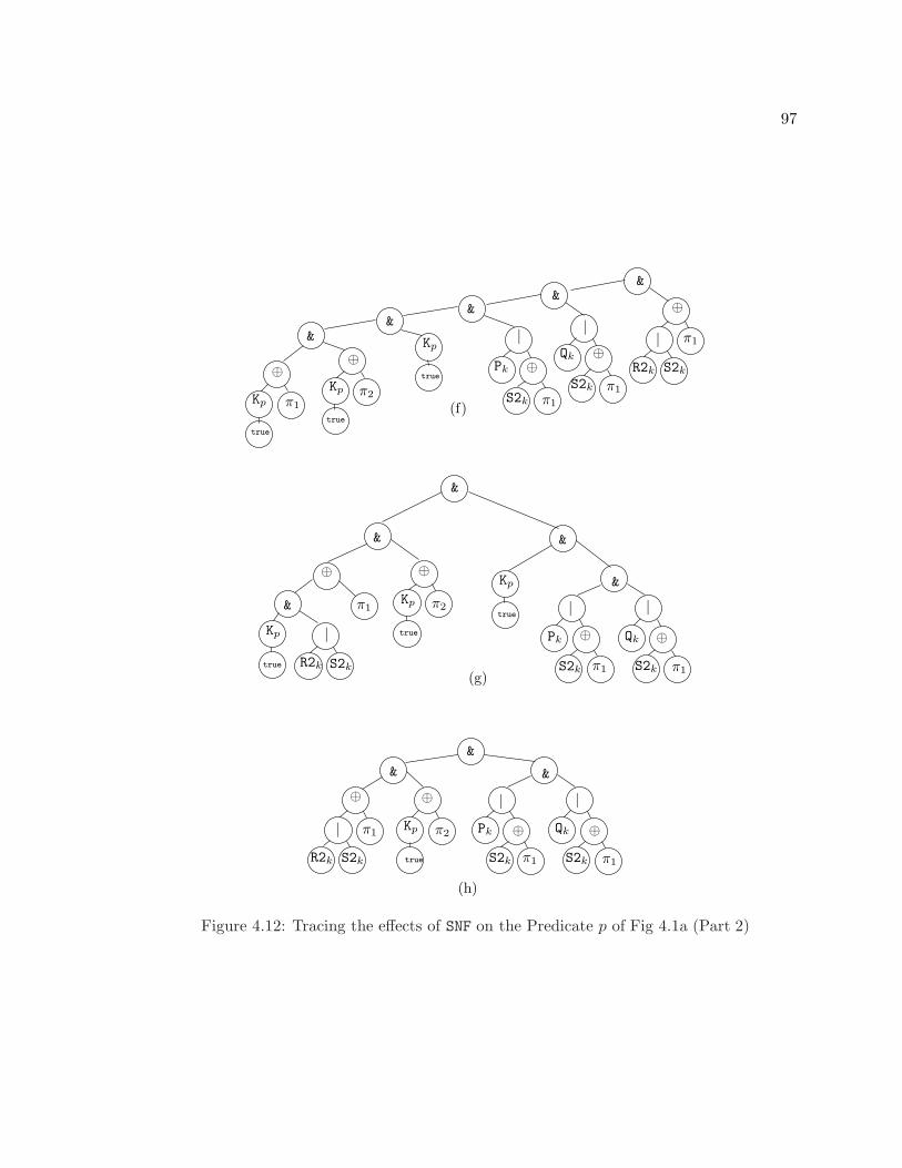
97
(h)
(g)
(f)
&
|R2k
⊕
S2k
π1
&
Qk ⊕|
π1S2k
&
Pk
S2k
|⊕
π1
&
Kp
true
&
π1
⊕Kp
true
⊕Kp π2
true
&
⊕Kp π2|
R2k
⊕
π1
S2k true
&
Qk⊕|
π1S2k
Pk
S2k
|⊕
π1
&
&
&
⊕
π1&
|R2k S2k
Kp
true
⊕Kp π2
true
&
Kp
true
Qk⊕|
π1S2k
Pk
S2k
|⊕
π1
&
Figure 4.12: Tracing the effects of SNF on the Predicate p of Fig 4.1a (Part 2)

98
that is “left-bushy” with respect to its parse tree. (Left-bushy conjunctions are defined
more formally in the next section.) This step prepares the predicate for the following step
that orders conjuncts. When applied to p4, LBConj returns the left-bushy conjunction,
p5 =((((((Kp (true) ⊕ π1) & (Kp (true) ⊕ π2)) & Kp (true)) &
(Pk | (S2k ⊕ π1))) & (Qk | (S2k ⊕ π1))) & ((R2k | S2k) ⊕ π1))
as illustrated in Figure 4.12f.
Step 6: This step fires the transformation OrderConjs shown in Figure 4.10. This trans-
formation performs a bottom-up pass, firing rules oc1, oc2 and oc3 on subtrees of the
form,
(p ⊕ π1) & (q ⊕ π2) & r & S
for predicates p, q, r and S. Because of step 3, the first subtree visited with this form has
p, q and r equal to Kp (true), and S equal to a conjunct from the original predicate. The
structure of S determines which rule gets fired:
• if S is of the form (s ⊕ π1), then s is merged with p by rule oc1 to form ((p & s) ⊕ π1).
• if S is of the form, (s ⊕ π2), then s is merged with q by rule oc2 to form ((q & s) ⊕ π2).
• if S is of any other form, then it is combined with r by rule oc3 to form (r & s).
The effect of this step on p5 is to transform it to
p6 = ((Kp (true) & ρk) ⊕ π1) & (σk ⊕ π2) & (Kp (true) & τk)
(as illustrated in Figure 4.12g) such that ρk, σk and τk are as defined in Figure 4.8.
Step 7: Finally, this step fires rule simp to get rid of the Kp (true) predicates that were
added in Step 3. (Note that σk of p6 above is not affected by this step.) The effect of
this step on p6 is to produce the final KOLA predicate of Figure 4.8 that is illustrated in
Figure 4.12h.
Correctness of SNF
Theorem 4.4.1 (Correctness) SNF is correct.
Proof: All query modification performed by SNF occurs as result of firing rules init, pull1,
. . ., pull4, and simp of transformation SNF; sft, sl1, . . . sl7, of transformation SimpLits;

99
sftp of transformation LBComp; d1, d2, involution, deMorgan1 and deMorgan2 of CNF; and
oc1, oc2, and oc3 of OrderConjs. Therefore, SNF is correct if these rules are correct. CNF’s
rules are proven correct by execution of the LP [46] theorem prover scripts of Appendix B.1.
All other rules are proven correct by execution of the LP [46] theorem prover scripts of
Appendix B.2. �
Proof that SNF succeeds in transforming KOLA qualification predicates into SNF is shown
by the lemmas and theorem below.
Lemma 4.4.1 (The Effect of SimpLits on Basic Functions) Let f be any basic func-
tion. Then SimpLits (f) will be a function of any of the forms shown below:
• f ◦ π1 (type 1),
• f ◦ π2 (type 2),
• Kf (x) (type 3), or
• f such that f is an inherently binary function (type 4).
Proof: (by induction on the height of f). For the base case, assume that f has height,
h ≤ 2. Then f must be either:
1. att ◦ π1,
2. att ◦ π2, or
3. Kf (x).
In any of these cases, no rules in SimpLits are fired and the functions are returned as is.
The returned functions are types 1, 2 and 3 respectively.
For the inductive case, f has height = k > 2, and therefore must be of the form,
op ◦ 〈f1, f2〉
for some function op and basic functions f1 and f2. Because SimpLits works bottom-up,
induction applies to f1 and f2 and therefore, by the time the root of f is visited, f1 and f2
will have been rewritten to one of types 1, 2, 3 or 4. We summarize all possible combinations
for f1 and f2 below:

100
Case 1 — f1 and f2 are type 3: Assume that f1 = Kf (x) and f2 = Kf (y). In
this case, rule sl1 fires on 〈f1, f2〉 leaving Kf ([x, y]). Subsequently, rule sl2 fires on
(op ◦ Kf ([x, y])) leaving
Kf (op ! 〈x, y〉)which is also type 3.
Case 2 — f1 and f2 are both type 1 or type 2: Let n be the type of f1 and f2. Assume that
f1 = f ′1 ◦ h and f2 = f ′2 ◦ h such that h = π1 or h = π2. In this case, rule sl5 fires on
〈f ′1 ◦ h, f ′2 ◦ h〉 leaving (〈f ′1, f ′2〉 ◦ h). Subsequently, rule sft fires on (op ◦ (〈f ′1, f ′2〉 ◦ h)),
leaving,
(op ◦ 〈f ′1, f ′2〉) ◦ h
which is type n.
Case 3 — One of f1 and f2 is type 3, and the other is type n (for n 6= 3): Suppose first
that f1 is type 3 and f2 = f ′2 ◦ h is type n. Then, rule sl4 fires on 〈f1, f2〉 leaving
〈g1, g2〉 ◦ (f ′2 ◦ h)
for some functions g1 and g2. Sft subsequently fires on this function leaving
(〈g1, g2〉 ◦ f ′2) ◦ h).
Sft fires again on
op ◦ (〈g1, g2〉 ◦ f ′2) ◦ h)
leaving
(op ◦ (〈g1, g2〉 ◦ f ′2)) ◦ h
which is type n.
A symmetric argument (such that sl3 is fired instead of sl4) handles the case where f2
is type 3.
Case 4 – One of f1 and f2 is type 4, or one is type 1 and the other is type 2: If one
of f1 or f2 is type 4, then no rules fire and 〈f1, f2〉 is inherently binary. No rules fire on
(op ◦ 〈f1, f2〉), and SimpLits returns this type 4 function.
If one of f1 or f2 is type 1 and the other is type 2, then no rules fire and again 〈f1, f2〉is inherently binary. No rules fire on (op ◦ 〈f1, f2〉), and SimpLits returns this type 4
function. �

101
Lemma 4.4.2 (The Effect of SimpLits on Pairs of Basic Functions) Let f1 and f2
be any basic functions. Then SimpLits (〈f1, f2〉) will be a function of one of the forms
shown below:
• f ◦ π1 (type 1),
• f ◦ π2 (type 2),
• Kf (x) (type 3), or
• f such that f is an inherently binary function (type 4).
Proof: Because SimpLits works bottom-up, f1 and f2 will be visited before 〈f1, f2〉. By
Lemma 4.4.1, when 〈f1, f2〉 is visited, both f1 and f2 will be of one of the following forms:
• f ◦ π1 (type 1),
• f ◦ π2 (type 2),
• Kf (x) (type 3), or
• f such that f is an inherently binary function (type 4).
The proof then proceeds by cases as before.
Case 1 — f1 and f2 are both type 3: Assume that f = Kf (x) and g = Kf (y). In this
case, rule sl1 fires on 〈f, g〉 leaving
Kf ([x, y])
which is type 3.
Case 2 — f1 and f2 are both type 1 or type 2: Let n be the type of f1 and f2. Assume
that f1 = f ′1 ◦ h and f2 = f ′2 ◦ h such that h = π1 or h = π2. In this case, rule sl5 fires
on 〈f ′1 ◦ h, f ′2 ◦ h〉 leaving
〈f ′1, f ′2〉 ◦ h,
which is type n.

102
Case 3 — One of f1 and f2 is type 3, and the other is type n (for n 6= 3): Suppose first
that f1 is type 3 and f2 = f ′2 ◦ h is type n. Then, rule sl4 fires on 〈f1, f2〉 leaving
〈g1, g2〉 ◦ (f ′2 ◦ h)
for some functions g1 and g2. Sft subsequently fires on this function leaving
(〈g1, g2〉 ◦ f ′2) ◦ h)
which is type n. A symmetric argument (such that sl3 is fired instead of sl4) handles the
case where f2 is type 3.
Case 4 – One of f1 and f2 is type 4, or one is type 1 and the other is type 2: If one of
f1 or f2 is type 4, then no rules fire and 〈f1, f2〉 is inherently binary (type 4). If one of f1
or f2 is type 1 and the other is type 2, then no rules fire and again 〈f1, f2〉 is inherently
binary (type 4). �
Lemma 4.4.3 (The Effect of SimpLits on Basic Predicates) Let p = q ⊕ f be any
basic predicate. Then SimpLits (p) will be a predicate of one of the following forms:
• p ⊕ π1 (type 1),
• p ⊕ π2 (type 2),
• Kp (b) (type 3), or
• p such that p is an inherently binary predicate (type 4).
Proof: Observe that the bottom-up pass of SimpLits ensures that f is visited before p.
Function f is of the form, 〈f1, f2〉 such that f1 and f2 are basic functions. By Lemma 4.4.2,
once p is visited during the bottom-up pass of SimpLits, it is of one of the forms below:
1. p ⊕ (f ◦ π1)
2. p ⊕ (f ◦ π2),
3. p ⊕ Kf (x), or
4. p ⊕ f such that f is inherently binary.
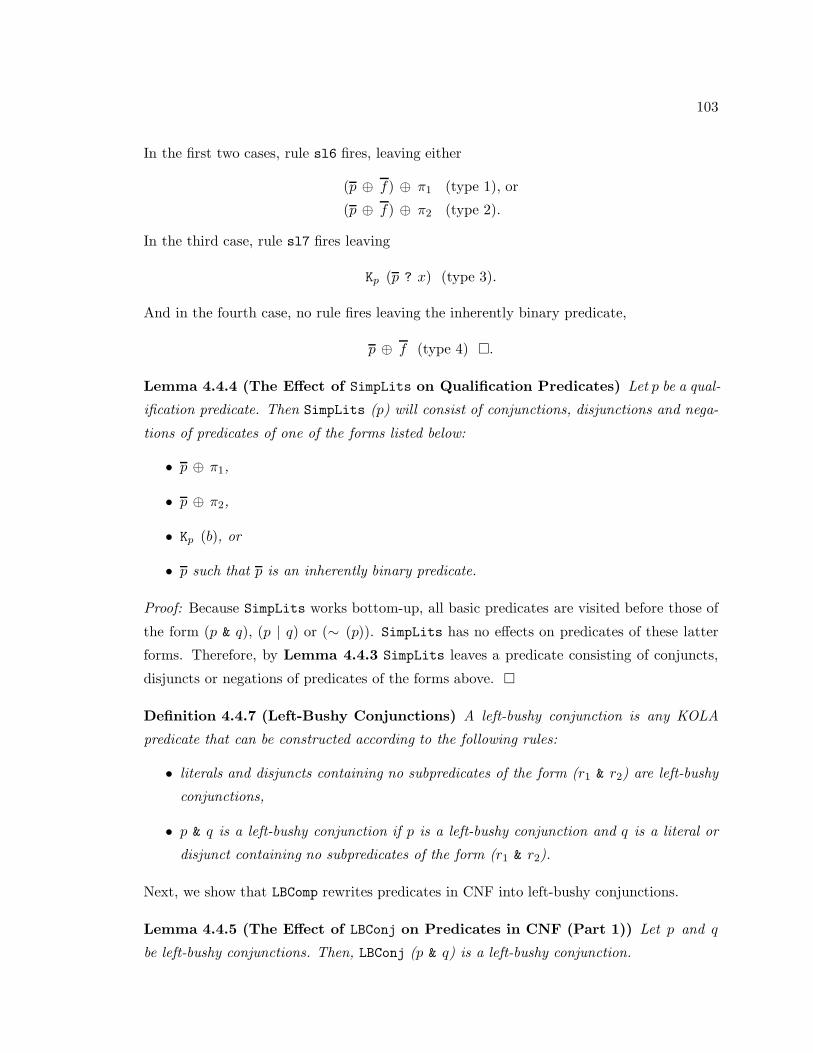
103
In the first two cases, rule sl6 fires, leaving either
(p ⊕ f) ⊕ π1 (type 1), or
(p ⊕ f) ⊕ π2 (type 2).
In the third case, rule sl7 fires leaving
Kp (p ? x) (type 3).
And in the fourth case, no rule fires leaving the inherently binary predicate,
p ⊕ f (type 4) �.
Lemma 4.4.4 (The Effect of SimpLits on Qualification Predicates) Let p be a qual-
ification predicate. Then SimpLits (p) will consist of conjunctions, disjunctions and nega-
tions of predicates of one of the forms listed below:
• p ⊕ π1,
• p ⊕ π2,
• Kp (b), or
• p such that p is an inherently binary predicate.
Proof: Because SimpLits works bottom-up, all basic predicates are visited before those of
the form (p & q), (p | q) or (∼ (p)). SimpLits has no effects on predicates of these latter
forms. Therefore, by Lemma 4.4.3 SimpLits leaves a predicate consisting of conjuncts,
disjuncts or negations of predicates of the forms above. �
Definition 4.4.7 (Left-Bushy Conjunctions) A left-bushy conjunction is any KOLA
predicate that can be constructed according to the following rules:
• literals and disjuncts containing no subpredicates of the form (r1 & r2) are left-bushy
conjunctions,
• p & q is a left-bushy conjunction if p is a left-bushy conjunction and q is a literal or
disjunct containing no subpredicates of the form (r1 & r2).
Next, we show that LBComp rewrites predicates in CNF into left-bushy conjunctions.
Lemma 4.4.5 (The Effect of LBConj on Predicates in CNF (Part 1)) Let p and q
be left-bushy conjunctions. Then, LBConj (p & q) is a left-bushy conjunction.

104
Proof: The proof is by induction on the number, n, of conjunctions in q. For the base
case, n = 0, (p & q) is already left-bushy and LBConj does nothing. In the inductive case,
q = q1 & q2. By the definition of left-bushy conjunctions, q1 is a left-bushy conjunction and
q2 is a literal or disjunct containing no subpredicates that are conjunctions. In this case,
rule sftp fires leaving,
(p & q1) & q2.
LBConj is subsequently fired on (p & q1) leaving, by induction, a left-bushy conjunction, p2.
Therefore, the predicate
p2 & q2
is also a left-bushy conjunction. �
Lemma 4.4.6 (The Effect of LBConj on Predicates in CNF (Part 2)) Let p be a pred-
icate in CNF. Then, LBConj (p) is left-bushy conjunction.
Proof: Because LBConj works bottom up, it visits p and q before it visits (p & q). A
simple inductive argument using Lemma 4.4.5 establishes LBConj to return a left-bushy
conjunction when fired on p. �
Theorem 4.4.2 (SNF) Given any KOLA qualification predicate p, SNF (p) is a predicate
in SNF.
Proof: The proof consists of seven parts, proving invariants that hold after the execution
of each step 1-7.
Invariant 1 : After firing SimpLits, p consists of conjunctions, disjunctions and nega-
tions of predicates of one of the forms listed below:
• p ⊕ π1 (type 1),
• p ⊕ π2 (type 2),
• Kp (b) (type 3),
• p such that p is an inherently binary predicate (type 4).
This invariant was shown to result from firing SimpLits by Lemma 4.4.4.

105
Invariant 2: After firing CNF, p is of the form,
p0 & . . . & pn
with each pi a disjunction of possibly negated literals of one of the four types listed in
Invariant 1. This invariant was shown to result from firing CNF in Section 4.2.3.
Invariant 3: After firing init, p is of the form,
(Kp (true) ⊕ π1) & (Kp (true) ⊕ π2) & (Kp (true)) & p1 & . . . & pn
with each pi disjunction of possibly negated literals of one of the four types listed in In-
variant 1.
Invariant 4: After executing BU {pull1 || pull2 || pull3 || pull4}, p is of the
form,
(Kp (true) ⊕ π1) & (Kp (true) ⊕ π2) & (Kp (true)) & q1 & . . . & qn
such that each qi is of any of the forms shown below:
• p ⊕ π1 (type 1),
• p ⊕ π2 (type 2),
• Kp (b) (type 3), or
• p such that p is an inherently binary predicate (type 4).
Note that none of the rewrite rules, pull1, . . ., pull4, affect the conjuncts at the top of the
tree, or the negations at the bottom. Rather, only disjuncts are affected. The proof then
is by induction on the height h of a disjunct (such that literals are viewed as having height
0). For the base case, h = 0 and no rules fire. In this case, we are left with a literal of types
1, 2, 3 or 4 (as listed in Invariant 1).
The induction proof considers the disjunct, p1 | p2 such that p1 and p2 are (by induction)
of types 1, 2, 3 or 4. The proof proceeds by cases:
• Case 1 — p1 and p2 are both type 1 or type 2: Let n be the type of p1 or p2. In this
case, rule pull1 fires and we are left with a type n predicate.
• Case 2 — p1 and p2 are both type 3: In this case, pull4 fires and we are left with a
type 3 predicate.
• Case 3 — One of p1 or p2 is type 4, or one is type 1 and the other is type 2: In this
case, no rule fires and we are left with a type 4 predicate.

106
Invariant 5: After firing LBConj, p is a left-bushy conjunction (as proven by Lemma 4.4.6).
Invariant 6: After firing OrderConjs, p will be of the form
(ρ ⊕ π1) & (σ ⊕ π2) & τ
such that τ is a conjunction of m (m ≥ 0) inherently binary or constant predicates (i.e., p
will be in SNF). Again, the proof of the invariant is by structural induction. exploiting the
bottom-up nature of OrderConjs. In the base case, OrderConjs is fired on
(Kp (true) ⊕ π1) & (Kp (true) ⊕ π2) & Kp (true),
doing nothing and leaving a predicate that is trivially in SNF.
Because p is a left-bushy conjunction, in the inductive case OrderConjs is fired on a
predicate of the form,
((((ρ ⊕ π1) & (σ ⊕ π2)) & τ) & p1
such that p1 is of one of the types listed in Invariant 4. If p1 is type 1, then it is merged
with ρ by rule oc1 to form (ρ & p1) ⊕ π1, leaving,
((ρ & p1) ⊕ π1) & (σ ⊕ π2) & τ
which is in SNF. If p1 is type 2, then it is merged with σ by rule oc2 to form (σ & p1) ⊕ π2,
leaving,
(ρ ⊕ π1) & ((σ & p1) ⊕ π2) & τ
which is in SNF. Finally, if p1 is type 3 or 4, then it is merged with τ by rule oc3 to form
(τ & p1), leaving,
(ρ ⊕ π1) & (σ ⊕ π2) & (τ & p1)
which is in SNF.
Invariant 7: After completion of the final step of the firing algorithm, we are left with a
predicate in SNF,
(ρ ⊕ π1) & (σ ⊕ π2) & τ
such that neither ρ, σ nor τ is of the for,
Kp (true) & p.
Satisfaction of this invariant follows trivially by examination of the rewrite rule, simp.

107
4.5 Example Applications of SNF
4.5.1 Example 3: Predicate-Pushdown
Figure 4.13 shows a COKO transformation that pushes predicates past joins. The key rule
of this transformation is push, which identifies subpredicates (p and q) of join predicates
that apply only to one argument, and pushes these subpredicates out of the join and onto
the join inputs. This heuristic is useful as it will usually result in a join of smaller collections.
Rule push will not fire successfully on every join query, for the predicate used in the
join may not be in a form that makes “pushable” subpredicates recognizable. For example,
if this rule were fired on the query,
join (p, π1) ! [Coms, SComs]
such that Coms and SComs are collections of committees and subcommittees respectively as
presented in Table 2.1, and p is the predicate of Figure 4.1a, it fails because this predicate
does not match the pattern,
(p ⊕ π1) & (q ⊕ π2) & r.
Therefore before this rule is fired, the predicate argument to join is normalized into SNF so
that “pushable” subpredicates can be identified. In the case of the predicate of Figure 4.1a,
normalization into SNF results in the query,
join ((ρ ⊕ π1) & (σ ⊕ π2) & τ , π1) ! [Coms, SComs]
such that ρ, σ and τ are as defined in Figure 4.8. Once in this form, firing push results in
join (τ , π1) ! [iterate (ρ, id) ! Coms, iterate (σ, id) ! SComs].
In this case, σ is Kp (true). Therefore, the subsequent firing of rule, simplify results in
the query,
join (τ , π1) ! [iterate (ρ, id) ! Coms, SComs].
4.5.2 Example 4: Join-Reordering
Figure 4.14 shows a COKO transformation that might be fired to change the order in which
multiple joins are evaluated. Transfomation Join-Associate reassociates a composition of
join queries. That is, a query of the form,
join (. . ., . . .) ! [join (. . ., . . .) ! [A, B], C]

108
TRANSFORMATION PushdownUSESSNF,
push: join ((p ⊕ π1) & (q ⊕ π2) & r, f) ! [A, B]→=
join (r, f) ! [iterate (p, id) ! A, iterate (q, id) ! B],
simplify: iterate (Kp (true), id) ! A→= A
BEGINGIVEN join (p, ) ! DO SNF (p);push;GIVEN ! [A, B] DO {simplify (A); simplify (B)}END
Figure 4.13: Pushdown: A COKO Transformation to Push Predicates Past Joins
gets rewritten to
join (. . ., . . .) ! [A, join (. . ., . . .) ! [B, C]].
Join-Associate first normalizes join predicates into SNF. The innermost join predicate
(q) gets normalized by SNF into,
(p2 ⊕ π1) & (q2 ⊕ π2) & r2.
The outermost join predicate (p) gets normalized by SNF into the form,
(p1 ⊕ π1) & (q1 ⊕ π2) & r1.
The innermost join predicate applies to pairs, [a, b] (for a ∈ A and b ∈ B). Therefore, p2
applies to a, q2 applies to b, and r2 applies to [a, b]. The outermost join predicate applies
to pairs, [f2 ! [a, b], c] (for f2 ! [a, b] in the result of the innermost join, and c ∈ C).
Therefore, p1 applies to f2 ! [a, b], q2 applies to c, and r3 applies to f2 ! [[a, b], c].
Firing shift on this normalized query results in a new query for which the innermost
join predicate and function are applied to pairs, [b, c] and and the outermost join predicate
and function are applied to pairs, [a, [b, c]]. Therefore, the rewrite rule places:
• (q2 ⊕ π1) in the innermost predicate because (q2 ⊕ π1) ? [b, c] = q2 ? b.
• (q1 ⊕ π2) in the innermost predicate because (q1 ⊕ π2) ? [b, c] = q1 ? c.
• (p2 ⊕ π1) in the outermost predicate because (p2 ⊕ π1) ? [a, [b, c]] = p2 ? a.
• (r2 ⊕ (id × π1)) in the outermost predicate because
(r2 ⊕ (id × π1)) ? [a, [b, c]] = r2 ? [a, b].

109
TRANSFORMATION Join-AssociateUSESshift: join ((p1 ⊕ π1) & (q1 ⊕ π2) & r1, f1) !
[join ((p2 ⊕ π1) & (q2 ⊕ π2) & r2, f2) ! [A, B], C]→=
join ((p1 ⊕ f1) & (r1 ⊕ h1) & (p2 ⊕ f2) & (r2 ⊕ h2), f1 ◦ h1) ![A, join ((q1 ⊕ g1) & (q2 ⊕ g2), id) ! [B, C]]
SNFBEGINGIVEN join (p, ) ! [join (q, ) ! [ , ], ] DO {SNF (p); SNF (q); shift}
END
such that
f1 = f2 ◦ (id × π1)g1 = π2
h1 = 〈f2 ◦ (id × π1), π2 ◦ π2〉f2 = π1
g2 = π1
h2 = id × π1
Figure 4.14: Join-Associate: A COKO Transformation to Reassociate a Join
• (p1 ⊕ (f2 ⊕ (id × π1))) in the outermost predicate because
(p1 ⊕ (f2 ⊕ (id × π1))) ? [a, [b, c]] = p1 ? (f2 ! [a, b]),
and
• (r1 ⊕ 〈f2 ◦ (id × π1), π2 ◦ π2〉) in the outermost predicate because
(r1 ⊕ 〈f2 ◦ (id × π1), π2 ◦ π2〉) ? [a, [b, c]] = r1 ? [f2 ! [a, b], c].
While the predicates that result from this rewrite are quite complex, in most cases they
can be simplified afterwards. For example, any subpredicates for which p1, q1, . . ., r2 is
Kp (true) can be made to drop away as a result of simplification.
4.6 Example 5: Magic-Sets
The idea behind the Magic-Sets transformation for relational queries introduced by Mumick
et al [74] is to restrict the inputs to a join by filtering those elements that cannot possibly
satisfy the join predicate. Therefore, this transformation is very much in the spirit of
predicate-pushdown, but passing filter predicates “sideways” from one join input to another,

110
SELECT cFROM c IN Coms, t in TempWHERE P (c, t) AND Q(c, t) AND R(c)
Temp (chair, avgTerms) =SELECT z.chair, AVG (SELECT m.terms FROM x IN partition, m IN x.mems)FROM z IN ComsGROUP BY z.chair
P (c, t) = c.chair == t.chairQ(c, t) = c.chair.terms > t.avgTerms
R(c) = c.chair.pty == ‘‘Dem’’
a. Before (OQL)
join (Pk & Qk & Rk, π1) ! [Coms, TempK]
TempK =njoin (eq ⊕ (id × chair), mems, avg ◦ flat) ![iterate (Kp (true), chair) ! Coms, Coms]
Pk = eq ⊕ 〈chair ◦ π1, π1 ◦ π2〉Qk = gt ⊕ 〈terms ◦ chair ◦ π1, π2 ◦ π2〉Rk = eq ⊕ 〈pty ◦ chair ◦ π1, Kf (‘‘Dem’’)〉
b. Before (KOLA)
Figure 4.15: OQL (a) and KOLA (b) queries to find all committees whose chair is a Demo-crat and has served more than the average number of terms of the members of his/herchaired committees.
rather than down from the join predicate. As with predicate-pushdown and join-reordering,
the magic-sets rewrite requires first normalizing the join predicate into SNF so that the
predicate that can be passed sideways can be identified.
4.6.1 An Example Magic-Sets Rewrite
Expressed in OQL
To illustrate, consider the OQL query of Figure 4.15a. This query returns the committees in
Coms that are chaired by someone who is a Democrat and who has served more terms than

111
SELECT c
FROM c IN MComs, t IN MTempWHERE P (c, t) AND Q(c, t)
MComs =SELECT m3FROM m3 IN MComsWHERE R(m3)
CSet (chair) =SELECT DISTINCT m2.chairFROM m2 IN MComs
MTemp (chair, avgTerms) =SELECT z.chair, AVG (SELECT m.terms FROM x IN partition, m IN x.mems)FROM z IN Coms, y IN CSetWHERE z.chair == y.chairGROUP BY z.chair
P (c, t) = c.chair == t.chairQ(c, t) = c.chair.terms > t.avgTermsR(m3) = m3.chair.pty == ‘‘Dem’’
c. After (OQL)
join (P ′k & Q′
k, π1) ! [MComsk, MTempk]
MComsk = iterate (R′k, id) ! Coms
CSetk = set ! (iterate (Kp (true), chair) ! MComsk)
MTempk = njoin (eq ⊕ (id × chair), mems, avg ◦ flat) ! [CSetk, Coms]
P ′k = eq ⊕ (chair × id) ⊕ (id × π1)
Q′k = gt ⊕ ((terms ◦ chair) × π2) ⊕ (id × π2)
R′k = eq ⊕ (〈id, Kf (‘‘Dem’’)〉 ◦ pty ◦ chair)
d. After (KOLA)
Figure 4.16: The queries of Figure 4.15 after rewriting by Magic-Sets
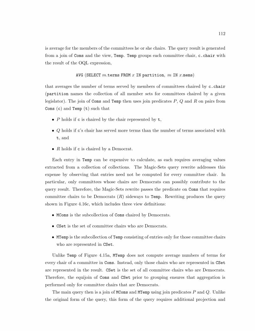
112
is average for the members of the committees he or she chairs. The query result is generated
from a join of Coms and the view, Temp. Temp groups each committee chair, c.chair with
the result of the OQL expression,
AVG (SELECT m.terms FROM x IN partition, m IN x.mems)
that averages the number of terms served by members of committees chaired by c.chair
(partition names the collection of all member sets for committees chaired by a given
legislator). The join of Coms and Temp then uses join predicates P , Q and R on pairs from
Coms (c) and Temp (t) such that
• P holds if c is chaired by the chair represented by t,
• Q holds if c’s chair has served more terms than the number of terms associated with
t, and
• R holds if c is chaired by a Democrat.
Each entry in Temp can be expensive to calculate, as each requires averaging values
extracted from a collection of collections. The Magic-Sets query rewrite addresses this
expense by observing that entries need not be computed for every committee chair. In
particular, only committees whose chairs are Democrats can possibly contribute to the
query result. Therefore, the Magic-Sets rewrite passes the predicate on Coms that requires
committee chairs to be Democrats (R) sideways to Temp. Rewriting produces the query
shown in Figure 4.16c, which includes three view definitions:
• MComs is the subcollection of Coms chaired by Democrats.
• CSet is the set of committee chairs who are Democrats.
• MTemp is the subcollection of Temp consisting of entries only for those committee chairs
who are represented in CSet.
Unlike Temp of Figure 4.15a, MTemp does not compute average numbers of terms for
every chair of a committee in Coms. Instead, only those chairs who are represented in CSet
are represented in the result. CSet is the set of all committee chairs who are Democrats.
Therefore, the equijoin of Coms and CSet prior to grouping ensures that aggregation is
performed only for committee chairs that are Democrats.
The main query then is a join of MComs and MTemp using join predicates P and Q. Unlike
the original form of the query, this form of the query requires additional projection and

113
duplicate elimination to generate CSet and an additional join to compute MTemp. However,
in many cases this additional cost is more than offset by the savings in not having to
compute average terms for committee chairs who are not Democrats.
Expressed in KOLA
Figures 4.15b and 4.16d show the KOLA equivalents of the OQL queries of Figures 4.15a and
4.16c respectively. The main query of Figure 4.15b performs a join of Coms and TempK (the
KOLA equivalent of Temp). The join predicate is the conjunction,
Pk & Qk & Rk
such that Pk is the KOLA equivalent to P and so on. The join function returns the first
element (the committee) of each pair, [c, t] (c ∈ Coms and t ∈ TempK) satisfying the join
predicate.
TempK is the KOLA equivalent of Temp, but for the naming of fields in the result. It
uses njoin to associate chairs of committees in Coms,
(iterate (Kp (true), chair) ! Coms)
with the sets of committees they chair. (For any committee chair l and committee c,
(eq ⊕ 〈π1, chair ◦ π2〉) ? [l, c]
holds if c is chaired by l.) For each committee c chaired by l, the set of c’s members (c.mems)
are added to an intermediate collection of legislator collections associated with l. Then, the
function, avg ◦ flat is applied to the result, first flattening this collection into a single
collection of legislators, and then averaging the number of terms they have served.
As with the OQL query of Figure 4.16c, the KOLA query of Figure 4.16d performs a join
of two new collections, MComsk and MTempk. The join predicate for this join is a conjunction
of predicates P ′k and Q′
k that are equivalent but transformed versions of predicates Pk and
Qk of Figure 4.15b. Like MComs, MComsk filters Coms for those commitees that satisfy R′k
(which is equivalent to Rk, but rewritten into a unary predicate). Like MTemp, MTempk
groups committees only if the committees are chaired by someone represented in CSetk
(CSet). And like CSet, CSetk determines the set of committee chairs for committees in
MComsk (MComs).

114
TRANSFORMATION MagicUSESSNF2, Pushdown, SimplifyJoins,
magic: join (q ⊕ (id × π1) & r, f) ! [A1, njoin (p, g, h) ! [A2, B]]→=
join (q ⊕ (id × π1) & r, f) ![A1, njoin (p, g, h) !
[set ! (join (q, π2) ! [A1, A2]), B]],
sftp: (p & q) & r→= p & (q & r)
BEGINPushdown; -- Step 1GIVEN join (p, ) ! DO {SNF2 (p); sftp (p)} -- Step 2magic -- Step 3GIVEN ! [ , A], A = ! [B, ] DO {SimplifyJoin (B)} -- Step 4
END
Figure 4.17: The Magic-Sets Rewrite Expressed in COKO
4.6.2 Expressing Magic-Sets in COKO
A COKO Magic-Sets transformation that converts the KOLA query of Figure 4.15b to that
of Figure 4.16d is shown in Figure 4.17. The key rewrite rule of this transformation is
magic, which assumes that a predicate argument to a join query has first been normalized
into the form
(q ⊕ (id × π1)) & r.
This normal form isolates the subpredicate, q, which relates elements of A1 and A2, as is
evident by tracing the evaluation of this predicate on any pair, [a1, [a2, S]] such that
a1 ∈ A1, and [a2, S] belongs to the result of the njoin subquery:
(q ⊕ (id × π1)) ? [a1, [a2, S]] = q ? [id ! a1, π1 ! [a2, S]]
= q ? [a1, a2].
Rule magic then rewrites the query so that q is used to “filter” elements of A2 so that
only those that relate to some element of A1 will be involved in the grouping and aggregate
computation performed by njoin. This filtering is expressed in the body pattern of magic
with the subexpression,
join (q, π2) ! [A1, A2]
which performs a right semi-join of A1 and A2 with respect to q. The elements of B that are
collected from this query are then freed of duplicates via a subsequent invocation of set.

115
Note that the semantics of njoin show that duplicate elimination on the result of the
semi-join is strictly not necessary (njoin ignores duplicates in the first collection argument).
The reason that rule magic introduces this unnecessary operator is to prepare this expres-
sion for simplification by transformation SimplifyJoin whose rewrite rules are listed in
Figure 4.3. Rule (8) of Figure 4.3 rewrites this semijoin into an intersection. But semijoins
can only be rewritten into intersections when the result of the semijoin is returned as a set.
Therefore, the operator set is introduced into the semijoin expression as an “indicator”
that duplicates in the result can be ignored.
Below we describe the steps performed by this transformation, demonstrating their
effects on the KOLA query of Figure 4.15b, and showing how they result in a rewrite of
this query to that shown in Figure 4.16d. In practice, translation into KOLA performs view
merging, and therefore the query of Figure 4.15b would be presented to the COKO Magic
transformation as Q0:
join (Pk & Qk & Rk, π1) !
[Coms, njoin (eq ⊕ (id × chair), mems, avg ◦ flat) !
[iterate (Kp (true), chair) ! Coms, Coms]]
such thatPk = eq ⊕ 〈chair ◦ π1, π1 ◦ π2〉Qk = gt ⊕ 〈terms ◦ chair ◦ π1, π2 ◦ π2〉, and
Rk = eq ⊕ 〈pty ◦ chair ◦ π1, Kf (‘‘Dem’’)〉
Steps 1 and 2:
The purpose of the first two steps of the transformation is to isolate that part of the
join predicate,
Pk & Qk & Rk
that is of the form
(q ⊕ (id × π1)) & r
to prepare it for firing by magic.
1. In Step 1, transformation pushdown (Section 4.5.1) is fired. Pushdown fires SNF on the
join predicate to convert it to the form,
(ρ ⊕ π1) & (σ ⊕ π2) & τ .

116
Then, ρ and σ are pushed out of the join. Applied to Q0, this step leaves Q1:
join (Pk & Qk, π1) !
[MComsk, njoin (eq ⊕ (id × chair), mems, avg ◦ flat) !
[iterate (Kp (true), chair) ! Coms, Coms]]
such thatMComsk = iterate (R′
k, id) ! Coms, and
R′k = eq ⊕ (〈id, Kf (‘‘Dem’’)〉 ◦ pty ◦ chair).
2. The second step normalizes τ by an SNF-like normalization. Transformation SNF2 is
similar to SNF, but rewrites τ into the form,
(α ⊕ (id × π1)) & (β ⊕ (id × π2)) & γ.
After these steps, the predicate is easily put into the desired form by setting q = α and
r = ((β ⊕ (id × π2)) & γ). This step prepares the predicate for a subsequent firing of rule
magic.
SNF2 is identical to SNF (Figure 4.9) but for the following exceptions:
1. Rather than firing SimpLits in Step 1, SNF2 fires the transformation SimpLits2 of
Figure 4.18.
2. Rather than firing rule init in Step 4, SNF2 fires the rule,
p→= (Kp (true) ⊕ (id × π1)) & (Kp (true) ⊕ (id × π2)) & Kp (true) & p.
3. Rather than firing OrderConjs in Step 6, SNF2 fires the transformation OrderConjs2
which fires the rules,
oc21 : (p ⊕ (id × π1)) & q & r & (s ⊕ (id × π1))→= ((p | s) ⊕ (id × π1)) & q & r,
oc22 : p & (q ⊕ (id × π2)) & r & (s ⊕ (id × π2))→= p & ((q | s) ⊕ π2) & r,
oc23 : p & q & r & s→= p & q & (r & s)
instead of rules oc1, oc2 and oc3 of Figure 4.10.
SimpLits2 adds transformation Pr2Times and rules sl8 – sl13 to the rules fired by
SimpLits. Pr2Times converts functions to products (f × g) where possible. Together with
the rules of SimpLits, rules sl8 – sl13 ensure that predicates on pairs [a, [b, S]] of the
form,
p = q ⊕ 〈f, g〉such that f and g are basic functions, are transformed into one of the forms shown below:

117
TRANSFORMATION SimpLits2USESPr2Times,
sft : f ◦ (g ◦ h) →= (f ◦ g) ◦ h
sl1 : 〈Kf (x), Kf (y)〉 →= Kf ([x, y]),sl2 : f ◦ Kf (x) →= Kf (f ! x),sl3 : 〈f, Kf (x)〉 →= 〈id, Kf (x)〉 ◦ f,
sl4 : 〈Kf (x), f〉 →= 〈Kf (x), id〉 ◦ f,
sl5 : 〈f ◦ h, g ◦ h〉 →= 〈f, g〉 ◦ h,
sl6 : p ⊕ (f ◦ g) →= p ⊕ f ⊕ g,
sl7 : p ⊕ Kf (x) →= Kp (p ? x),sl8 : 〈f ◦ π1, g ◦ (id × h)〉 →= 〈f ◦ π1, g〉 ◦ (id × h),sl9 : 〈f ◦ (id × h), g ◦ π1〉 →= 〈f, g ◦ π1〉 ◦ (id × h),sl10 : 〈f ◦ (h ◦ π2), g ◦ (id × h)〉 →= 〈f ◦ π2, g〉 ◦ (id × h),sl11 : 〈f ◦ (id × h), g ◦ (h ◦ π2)〉 →= 〈f, g ◦ π2〉 ◦ (id × h),sl12 : 〈f ◦ (g ◦ π2), g ◦ π2〉 →= 〈f ◦ g, h〉 ◦ π2,
sl13 : 〈f ◦ π2, h ◦ (h ◦ π2)〉 →= 〈f, h ◦ g〉 ◦ π2,BEGINBU {Pr2Times || sl1 || sl2 || {{sl3 || sl4} → REPEAT sft} || sl5 || sl6 || sl7 ||
sl8 || sl9 || sl10 || sl11 || sl12 || sl13 || REPEAT sft}END
TRANSFORMATION Pr2TimesUSES
co1 : 〈f ◦ π1, g ◦ (h ◦ π2)〉 →= (f × g) ◦ (id × h),co2 : 〈f ◦ (h ◦ π2), g ◦ π1〉 →= 〈π2, π1〉 ◦ (f × g) ◦ (id × h),co3 : 〈f ◦ (π1 ◦ π2), g ◦ (π2 ◦ π2)〉 →= (f × g) ◦ π2,
co4 : 〈f ◦ (π2 ◦ π2), g ◦ (π1 ◦ π2)〉 →= 〈π2, π1〉 ◦ (f × g) ◦ π2,
co5 : 〈f ◦ π1, g ◦ π2〉 →= (f × id) ◦ (id × g),co6 : 〈f ◦ π2, g ◦ π1〉 →= 〈π2, π1〉 ◦ (f × id) ◦ (id × g),co7 : 〈π1, π2〉 →= id,
co8 : f ◦ id →= f,
co9 : id ◦ f→= f
BEGINBU {co1 || co2 || co3 || co4 || co5 || co6 || co7 || co8 || co9}END
Figure 4.18: Transformation SimpLits2 and its Auxiliary Transformation Pr2Times

118
• Kp (b) (if q ignores its inputs),
• p ⊕ π1 (if q only requires a),
• p ⊕ π2 (if q only requires b and S),
• p ⊕ (id × π1) (if q only requires a and b),
• p ⊕ (id × π2) (if q only requires a and S).
When fired on Pk, rule co5 transforms the function,
〈chair ◦ π1, π1 ◦ π2〉
into
(chair × id) ◦ (id × π1).
Then, rule pr1 fires leaving the predicate
eq ⊕ (chair × id) ⊕ (id × π1).
When fired on Qk, rule co5 transforms the function,
〈terms ◦ chair ◦ π1, π2 ◦ π2〉
into
((terms ◦ chair) × id) ◦ (id × π2).
Then, rule pr1 fires leaving the predicate
gt ⊕ ((terms ◦ chair) × id) ⊕ (id × π2).
All subsequent steps in SimpLits2 are as in SimpLits. Therefore, the the result of firing
SimpLits2 on Q1 is the query, Q2:
join ((α ⊕ (id × π1)) & ((β ⊕ (id × π2)) & γ), π1) !
[MComsk, njoin (eq ⊕ (id × chair), mems, avg ◦ flat) !
[iterate (Kp (true), chair) ! Coms, Coms]]
such thatα = eq ⊕ (chair × id), and
β = gt ⊕ ((terms ◦ chair) × id), and
γ = Kp (true).

119
After SNF2 is fired, rule sftp is fired to reassociate the three conjunct join subpredicates,
((α ⊕ (id × π1)) & (β ⊕ (id × π2))) & γ
into
(α ⊕ (id × π1)) & ((β ⊕ (id × π2)) & γ).
This firing prepares the predicate for the firing of rule magic in the next step. The result
of firing sftp on Q2 is Q3:
join ((q ⊕ (id × π1)) & r, π1) !
[MComsk, njoin (eq ⊕ (id × chair), mems, avg ◦ flat) !
[iterate (Kp (true), chair) ! Coms, Coms]]
such that
q = eq ⊕ (chair × id), and
r = ((gt ⊕ ((terms ◦ chair) × id)) ⊕ (id × π2)) & Kp (true).
Step 3:
Next, rewrite rule magic is fired. This rule introduces the left join argument (A1) into
the right-hand side of the join. Firing magic makes it possible to restrict the input (A2) to
njoin to elements that are related by q to A1. Fired on Q3, magic leaves Q4:
join ((q ⊕ (id × π1)) & r, π1) !
[MComsk, njoin (eq ⊕ (id × chair), mems, avg ◦ flat) ! [CSet′k, Coms]]
or equivalently,
join (P ′k & Q′
k, π1) !
[MComsk, njoin (eq ⊕ (id × chair), mems, avg ◦ flat) ! [CSet′k, Coms]]
such that
CSet′k = set ! (join (eq ⊕ (chair × id), π2) !
[MComsk, iterate (Kp (true), chair) ! Coms]),
MComsk = iterate (R′k, id) ! Coms,
P ′k = eq ⊕ (chair × id) ⊕ (id × π1), and
Q′k = gt ⊕ ((terms ◦ chair) × π2) ⊕ (id × π2)

120
1. (id × id) →= id2. p ⊕ id →= p
3. Kp (true) ⊕ f→= Kp (true)
4. p & Kp (true) →= p
5a. f ◦ id →= f
5b. id ◦ f→= f
6. (f × g) ◦ (h × j) →= (f ◦ h) × (g ◦ j)7. p ⊕ f ⊕ g
→= p ⊕ (f ◦ g)8. set ! (join (eq, π2) ! [A, B]) →= set ! (A ∩ B)
9. join (p ⊕ (f × g), π2) ! [A, B]→=
join (p ⊕ (id × g), π2) ! [iterate (Kp (true), f) ! A, B]
10. iterate (p, f) ! (iterate (q, g) ! A) →= iterate (q & (p ⊕ g), f ◦ g) ! A
11. (iterate (p, f) ! A) ∩ (iterate (Kp (true), f) ! A) →= iterate (p, f) ! A
12. njoin (p, f, g) ! [set ! A, B]→= njoin (p, f, g) ! [A, B]
13. iterate (p, f) ! A→= iterate (Kp (true), f) ! (iterate (p, id) ! A)
Table 4.3: Rewrite Rules Used In SimplifyJoin
Step 4:
Step 4 fires transformation SimplifyJoin on the semijoin expression resulting from the
previous step. SimplifyJoin uses the rules of Table 4.3 to rewrite CSet′k into CSetk (of
Figure 4.16d) as we show below:
• The first rule fired is rule 9, which rewrites CSet′k,
set ! (join (eq ⊕ (chair × id), π2) !
[MComsk, iterate (Kp (true), chair) ! Coms])
to
set !
(join (eq ⊕ (id × id), π2) !
[iterate (Kp (true), chair) ! MComsk, iterate (Kp (true), chair) ! Coms]).
• Firing rules 1 and 2 simplifies the join predicate, leaving
set !
(join (eq, π2) !
[iterate (Kp (true), chair) ! MComsk, iterate (Kp (true), chair) ! Coms]).

121
• Expanding for MComsk and firing rules 10, 3, 4 and 5a, leaves
set !
(join (eq, π2) !
[iterate (R′k, chair) ! Coms, iterate (Kp (true), chair) ! Coms]).
• Next, rule 8 fires, converting the right semijoin to an intersection. Firing rule 8 leaves:
set ! ((iterate (R′k, chair) ! Coms) ∩ (iterate (Kp (true), chair) ! Coms)).
• This expression in turn reduces by firing rule 11 to:
set ! (iterate (R′k, chair) ! Coms),
which then gets split up by firing rule 13 to:
set ! (iterate (Kp (true), chair) ! (iterate (R′k, id) ! Coms))
= set ! (iterate (Kp (true), chair) ! MComsk)
= CSetk.
Therefore, after SimplifyJoin has finished firing, we are left with the query of Fig-
ure 4.16d:
join (P ′k & Q′
k, π1) ! [MComsk, MTempK]
such that MTempK is:
njoin (eq ⊕ (id × chair), mems, avg ◦ flat) ! [CSetk, Coms].
4.7 Discussion
4.7.1 The Expressivity of COKO
COKO is still evolving. Our goal is to reach a point with it where we are able to express
all of the useful query rewrites that can be expressed with a programming language with-
out compromising the separation of rewrite rules from firing algorithms. To this end, our
design process alternates between modifying the language and using it to express complex
query rewrites. In this chapter, we have presented some of the rewrites that we have gener-
ated with COKO, including CNF (exhaustive and non-exhaustive versions), SNF, Pushdown,
Join-Associate and Magic.

122
Though COKO is evolving, it is not immature. We believe that COKO already pro-
vides most of the useful idioms required to express query rewriting. By combining COKO
statements in varying ways, we are able to express such common firing algorithms as
• BU {r1 || . . . || rn}:fire every rule r1, . . ., rn succesively on every subtree,
• BU r1; . . . BU rn:
fire every rule r1, . . ., rn on every succesive subtree,
• BU {{REPEAT r1}; . . .; {REPEAT rn}}:fire every rule r1, . . ., rn repeatedly on every successive subtree,
• S → S ′ || S ′′:
execute S and then S ′ if S succeeds and S ′′ if S fails, and
• S → recursive fire:
execute S exhaustively.
As before, attempts to express transformations drive the design of the language. Provided
that we are able to maintain the separation of rewrite rules from firing algorithms, we are
prepared to let COKO evolve into a steady and usable state.
4.7.2 The Need for Normalization
The CNF and SNF query rewrites are normalizations: query rewrites that convert expres-
sions into syntactically characterizable (i.e., normal) forms. Normalizations epitomize the
kinds of complex query rewrites that cannot be expressed as rewrite rules and that typically
get expressed with code.
Normalization gets little attention in the optimizer literature. And yet, normaliza-
tion can be more complex, expensive and error-prone than the optimizations they preceed.
(Consider that Kim’s erroneous rewrites are normalizations whose normal forms are join
queries.) In the context of object-oriented and object-relational databases, normalization
assumes even greater importance. Firstly, nested object queries are far more prevalent and
can be more deeply nested than relational queries making their normalization more diffi-
cult and more urgent. Secondly, because many object databases are built as extensions
of existing systems (e.g., object-relational extensions of relational systems), normalization

123
affords the opportunity to rewrite complex (e.g., object) queries into a series of simpler
(e.g., relational) queries that can be posed of the original query engine. (We will see an
example of this object → relation translation in Chapter 6.)
We have shown with two examples (CNF and SNF) that COKO is capable of expressing
complex normalizations that typically get expressed only with code. For both normaliza-
tions, we were able to show not only correctness, but also prove that the firing algorithms for
these transformations did as they were intended. Neither of these results is straightforward
when the normalizations are expressed with code, even when the normalizations themselves
have more straightforward expression with code.5 Therefore, the correctness results arising
from the COKO-KOLA approach come at a complexity cost for expressing certain rewrites.
In designing future versions of COKO, our goal will be to make firing algorithms simpler to
formulate, in order to lower this cost.
4.8 Chapter Summary
In this chapter, we introduced a language (COKO) for defining transformations: complex
query rewrites for rule-based optimizers. COKO transformations generalize rewrite rules.
Like rules, they can be fired and can succeed or fail as a result. But because they are
expressed algorithmically, they are able to express many rewrites (such as normalizations)
that rewrite rules cannot.
A COKO transformation consists of a set of rewrite rules and a firing algorithm spec-
ifying how they are fired. The separation of rewriting (expressed with rewrite rules) and
firing control (expressed with firing algorithms) makes it possible to express complex and
efficient rewrites that can still (because rewrite rules are over KOLA queries) be verified
with a theorem prover.
COKO transformations can be made efficient and expressive. The language for firing
algorithms includes the kinds of operators that are most useful for describing rewrites.
These include explicit rule firing, traversal control, selective firing and conditional firing.
We demonstrated the efficiency benefits of firing algorithms with an example COKO trans-
formation that converts predicates to CNF. We demonstrated the expressivity of COKO
with numerous examples that typically do not get expressed with declarative rewrite rules.
These examples included a complex normalization (SNF) and three complex rewrites that5SNF for example, is straightforward to express with code that 1) converts a binary predicate to CNF,and 2) traces the origins of all attributes appearing in each conjunct to see which conjuncts involveattributes only from the first input, second input or both.
124
depend on it (predicate-pushdown, join-reordering and Magic-Sets rewrites).
COKO extends and generalizes KOLA. Whereas KOLA used a modular approach to
build queries from functions, COKO uses a modular approach to build complex query
rewrites from rewrite rules. This modular approach facilitates the verification of query
rewriters.
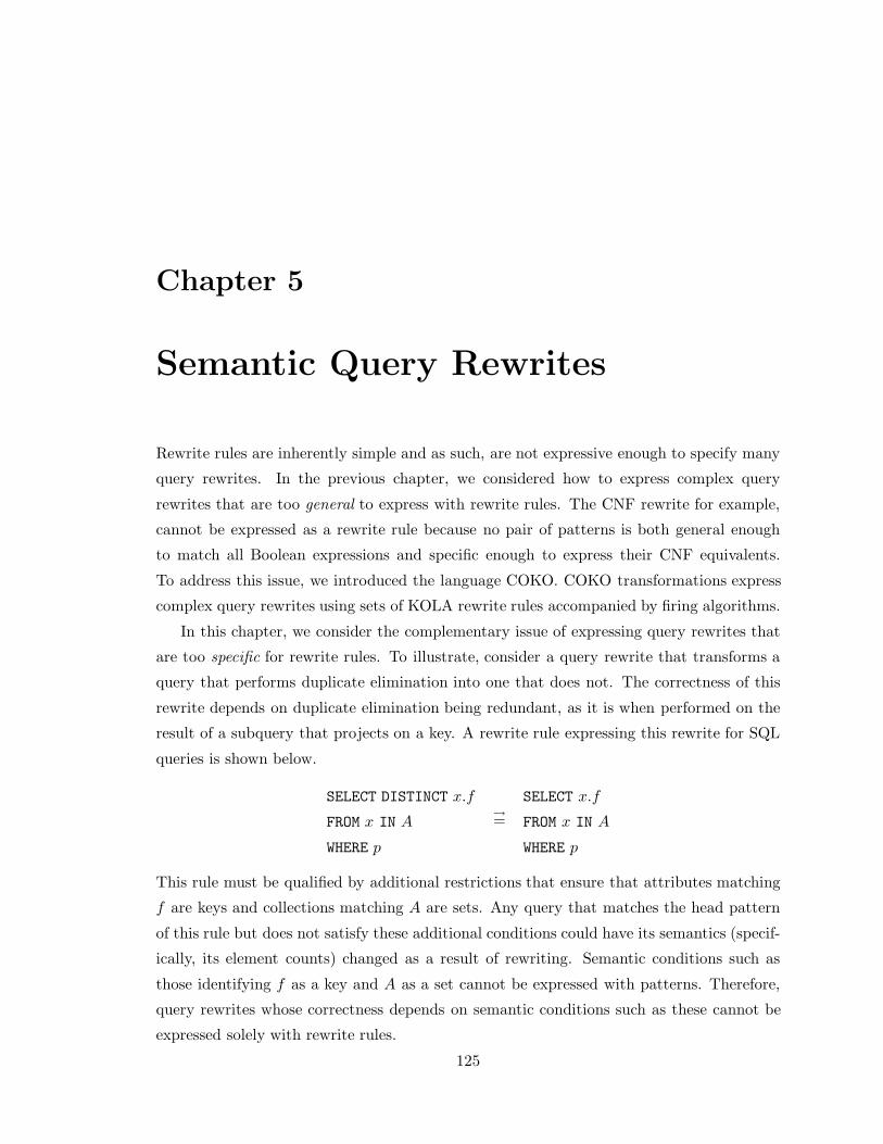
Chapter 5
Semantic Query Rewrites
Rewrite rules are inherently simple and as such, are not expressive enough to specify many
query rewrites. In the previous chapter, we considered how to express complex query
rewrites that are too general to express with rewrite rules. The CNF rewrite for example,
cannot be expressed as a rewrite rule because no pair of patterns is both general enough
to match all Boolean expressions and specific enough to express their CNF equivalents.
To address this issue, we introduced the language COKO. COKO transformations express
complex query rewrites using sets of KOLA rewrite rules accompanied by firing algorithms.
In this chapter, we consider the complementary issue of expressing query rewrites that
are too specific for rewrite rules. To illustrate, consider a query rewrite that transforms a
query that performs duplicate elimination into one that does not. The correctness of this
rewrite depends on duplicate elimination being redundant, as it is when performed on the
result of a subquery that projects on a key. A rewrite rule expressing this rewrite for SQL
queries is shown below.
SELECT DISTINCT x.f
FROM x IN A
WHERE p
→=SELECT x.f
FROM x IN A
WHERE p
This rule must be qualified by additional restrictions that ensure that attributes matching
f are keys and collections matching A are sets. Any query that matches the head pattern
of this rule but does not satisfy these additional conditions could have its semantics (specif-
ically, its element counts) changed as a result of rewriting. Semantic conditions such as
those identifying f as a key and A as a set cannot be expressed with patterns. Therefore,
query rewrites whose correctness depends on semantic conditions such as these cannot be
expressed solely with rewrite rules.
125

126
As with complex query rewrites, existing rule-based systems address this expressivity is-
sue by replacing or supplementing rewrite rules with code. Whereas complex query rewrites
use code to manipulate matched expressions in ways that cannot be expressed with patterns,
semantic query rewrites use code to test semantic conditions of expressions that successfully
unify. For example, the SQL transformation above that eliminates duplicate removal would
be expressed in Starburst [79] with C code that examined annotations of the underlying
query representation (QGM) to decide if a matched attribute was a key and if a matched
collection was a set.
This chapter proposes an alternative approach for expressing semantic query rewrites
that is consistent with our goal of making query rewriters verifiable with a theorem prover.
As with COKO, this work builds upon the KOLA work introduced in Chapter 3. We add
two new kinds of rules to the COKO-KOLA framework:
• Conditional rewrite rules, and
• Inference rules.
Conditional rewrite rules resemble (unconditional) rewrite rules, except that when they are
fired, the match of the rule’s head pattern to a query expression is followed by analysis to
see if certain conditions hold of identified subexpressions. Inference rules tell the optimizer
how to decide if these conditions hold.
The contributions of the work presented in this chapter are:
1. Verifiable Semantic Query Rewrites: In keeping with our goal outlined in Chapter 1,
all query rewrites specifiable with inference and conditional rewrite rules are verifiable
with a theorem prover.
2. Use of Inference Rules to Infer Query Semantics: This work is unique in its use of
inference rules to specify semantic conditions. This technique separates the rules that
depend on semantic conditions (conditional rewrite rules) from the decision-making
process that decides if these semantic conditions hold. Our approach is distinct from
that of existing rule-based systems that embed decision-making code within the rule
that may or may not fire as a result.
The use of inference rules to specify semantic conditions makes optimizers extensible
in ways that standard rule-based optimizers are not. By modifying a set of rewrite rules
used by an optimizer, one can change how a query gets rewritten. On the other hand, by

127
modifying a set of inference rules used by an optimizer, one can change when rewrite rules
predicated on inferred conditions get fired.
The rest of this chapter proceeds as follows. In Section 5.1, we motivate this work by
presenting queries over the Thomas database, and showing how the semantics of their data
functions (in this case, their injectivity) can be inferred and exploited for rewriting. In this
section, we also show how the conditional rewrite rules and inference rules that specify these
semantic rewrites would be expressed within COKO-KOLA. Section 5.2 presents a second
example of a semantic condition (predicate strength) that can be used as a condition for
many useful semantic rewrites. Section 5.3 describes how our COKO compiler was modified
to account for inference and conditional rewrite rules. Section 5.4 discusses issues that arose
in the design and implementation of this compiler extension, and a chapter summary follows
in Section 5.5.
The semantic query rewrites presented in this chapter are not new. The injectivity-based
rewrites of Section 5.1 have been discussed in numerous texts (e.g., Ullman’s introductory
text on databases [95]). The predicate strength rewrites of Section 5.2 are similar to the
predicate “move-around” rewrites introduced by Levy, et al. [71]. Our work is unique
in its declarative expression of these rewrites that makes them verifiable with a theorem
prover. Further, the use of inference rules to define these conditions makes rule-based query
rewriters extensible in ways that have not been proposed before.
5.1 Example 1: Injectivity
Figures 5.1a and 5.1b show two simple OQL queries over the Thomas database. The “Major
Cities” query (Figure 5.1a) queries a set of House Representatives (HReps) applying the path
expression, x.reps.lgst cit, to each. The result of this query is the collection of cities that
are the largest of those located in the districts represented by House Representatives in
HReps, with duplicate cities removed.1 The “Mayors” query (Figure 5.1b) also queries a set
of House Representatives. For each Representative, this query returns the mayors of major
cities located in the district that the Representative represents (this time, with duplicate
mayor collections removed from the result).
The “Major Cities” query and the “Mayors” query can be evaluated in similar ways: by
first retrieving House Representatives in HReps, applying a data function to each to generate1As we mentioned in Chapter 2, we make the simplifying assumption that cities are located in only oneCongressional district. While this may not be the case in practice, we can enforce this assumption byassigning every city to that district where a majority of its inhabitants reside.
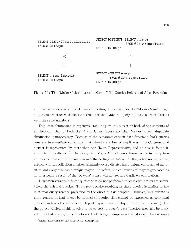
128
SELECT DISTINCT x.reps.lgst citFROM x IN HReps
SELECT DISTINCT (SELECT d.mayorFROM d IN x.reps.cities)
FROM x IN HReps
(a) (b)
↓ ↓
SELECT x.reps.lgst citFROM x IN HReps
SELECT (SELECT d.mayorFROM d IN x.reps.cities)
FROM x IN HReps
Figure 5.1: The “Major Cities” (a) and “Mayors” (b) Queries Before and After Rewriting
an intermediate collection, and then eliminating duplicates. For the “Major Cities” query,
duplicates are cities with the same OID. For the “Mayors” query, duplicates are collections
with the same members.
Duplicate elimination is expensive, requiring an initial sort or hash of the contents of
a collection. But for both the “Major Cities” query and the “Mayors” query, duplicate
elimination is unnecessary. Because of the semantics of their data functions, both queries
generate intermediate collections that already are free of duplicates. No Congressional
district is represented by more than one House Representative, and no city is found in
more than one district.2 Therefore, the “Major Cities” query inserts a distinct city into
its intermediate result for each distinct House Representative. As HReps has no duplicates,
neither will this collection of cities. Similarly, every district has a unique collection of major
cities and every city has a unique mayor. Therefore, the collections of mayors generated as
an intermediate result of the “Mayors” query will not require duplicate elimination.
Rewritten versions of these queries that do not perform duplicate elimination are shown
below the original queries. The query rewrite resulting in these queries is similar to the
relational query rewrite presented at the onset of this chapter. However, this rewrite is
more general in that it can be applied to queries that cannot be expressed as relational
queries (such as object queries with path expressions or subqueries as data functions). For
the object version of this rewrite to be correct, a query’s data function need not be a key
attribute but any injective function (of which keys comprise a special case). And whereas2Again, according to our simplifying assumption.

129
set ! (iterate (Kp (true), f) ! HReps)s.t.: f = lgst cit ◦ reps
↓iterate (Kp (true), f) ! HReps
s.t.: f = lgst cit ◦ reps
KOLA Equivalents of the “Major Cities” Query (Before and After Rewriting)
set ! (iterate (Kp (true), f) ! HReps)s.t.: f = iterate (Kp (true), mayor) ◦ cities ◦ reps
↓iterate (Kp (true), f) ! HReps
s.t.: f = iterate (Kp (true), mayor) ◦ cities ◦ reps
KOLA Equivalents of the “Mayors” Query (Before and After Rewriting)
Figure 5.2: KOLA Translations of Figures 5.1a and 5.1b
a relational query rewriter need only consult metadata files (e.g., the database schema) to
determine whether a query’s data function is a key, this approach is inadequate for deciding
the injectivity of functions that might appear in object queries. The number of injective path
expressions alone might be very large and even infinite. (Aside from x.reps.lgst cit, other
injective path expressions on House Representatives are x.name, x.reps, x.reps.cities,
x.reps.lgst cit.mayor and so on.) Thus, it is unlikely that metadata files can be scaled to
keep track of all injective data functions, and inference is required instead.
Figure 5.2 shows KOLA equivalents of the “Major Cities” query and “Mayors” query
both before and after the application of a semantic query rewrite to remove duplicate
elimination (set). The KOLA translations of the data functions (f) for these two queries
are:
• lgst cit ◦ reps, equivalent to the “Major Cities” query path expression,
x.reps.lgst cit,
and
130
• iterate (Kp (true), mayor) ◦ cities ◦ reps, equivalent to the “Mayors” query sub-
query,SELECT d.mayor
FROM d IN x.reps.cities.
5.1.1 Expressing Semantic Query Rewrites in COKO-KOLA
To express semantic rewrites in COKO, we introduce two new kinds of declarative rules to
the language:
• Conditional Rewrite Rules resemble (unconditional) rewrite rules, but can include
semantic conditions on the subexpressions of matched query expressions. These con-
ditions can, for example, indicate that a given KOLA function must be injective or
that a given KOLA collection must be a set. Like unconditional rules, conditional
rewrite rules can be fired within COKO transformations.
• Inference Rules specify how semantic conditions can be inferred of KOLA functions,
predicates, objects and collections. A property is a set of rules that can be used to
infer the same condition. We have modified our COKO compiler to compile properties
into code that gets executed during rule firing.
Conditional Rewrite Rules in COKO
Conditional rewrite rules have the form,
C :: L→= R
such that L and R are patterns of KOLA expressions (i.e., such that L→= R is an un-
conditional rewrite rule), and C is a set of semantic conditions that must hold of various
subexpressions of query expressions that unify with L. Figure 5.3 shows two example con-
ditional rewrite rules that eliminate redundant duplicate elimination. Inj1 can be fired on
either the “Major Cities” query or the “Mayors” query. (Inj2 will be discussed in Sec-
tion 5.1.3.) The head pattern of this rule matches queries that remove duplicates (with
set) from the results of iterate queries. The rule’s body pattern shows the same query
as the rule’s head pattern, but with the invocation of set removed. The conditions of the
rule state that the rule is correct provided that function f is injective and collection A is a
set. Therefore, conditional rewrite rules specify query rewrites that should only be fired if
certain conditions hold.

131
inj1 : is inj (f), is set (A) ::set ! (iterate (p, f) ! A) →= iterate (p, f) ! A
inj2 : is inj (f), is set (g ! ) ::set ◦ iterate (p, f) ◦ g
→= iterate (p, f) ◦ g
Figure 5.3: Conditional Rewrite Rules to Eliminate Redundant Duplicate Elimination
Inference Rules (Properties) in COKO
To perform a query rewrite that removes redundant duplicate elimination, a rewriter must
determine that a query’s data function is injective and that a collection is a set. Like
most semantic properties of functions, injectivity is undecidable in general. Determination
of whether or not a given collection is a set could be made at runtime, but this requires
processing (sorting the collection and scanning for duplicates) that the conditional rewrite
rules of Figure 5.3 are intended to avoid. Therefore, it is not realistic to assume that a
complete reasoning system for user-defined properties is possible or even desirable. But
with guidance, a rewriter can infer that properties such as injectivity hold in some cases.
Incomplete inference is preferable to not performing inference at all for at least in these cases,
rewriting might improve the evaluation of the query. Therefore, we care about soundness
and not about completeness in inferring semantic properties.
Guidance comes from two sources:
• metadata provided by the user that declares object types, integrity (including key)
constraints, etc., and
• inference rules defined by the optimizer developer.
For example, a user might state that a particular attribute of a type is a key.3 As well,
a user might identify the types of objects that are globally named, thus identifying some
named collections as sets and others as bags. The depth and accuracy of the information
supplied by the user determines the quality and correctness of rewriting.3In the relational world, a key is typically thought of as a property of a collection (i.e., a relation) ratherthan a property of a type. However, relations are often used to represent the extent of a type and in thiscase the association of key with type is natural. Further, equality definitions for types must be definedin terms of keys for sets of objects of that type to be well-behaved. (See our DBPL ’95 paper [23] forthe argument as to why this is so.) Therefore, keys can be thought of as properties of types and notjust collections.

132
The inference rules supplied to the optimizer enable inference of conditions that are
not explicitly stated. For example, a user might identify lgst cit and reps as being key
attributes for sets of Congressional districts and House Representatives respectively, but is
unlikely to identify longer path expressions (such as x.reps.lgst cit) as keys given that
there can be too many path expressions to anticipate and consider. But an inference rule
can be used to infer that a path expression is injective given that each of the attributes in
its path is a key. Or, it can be used to infer that a tuple construction is injective if any of
its fields is derived from a key.
A rewriter constructed using the COKO compiler could infer that some functions are
injective according to the inference rules defined in the property definitions of Figure 5.4a.
Inference rules have the form,
body =⇒ head
(or just head which states a fact that is unconditionally true). The head of an inference
rule names a condition (e.g., is inj (f)) to infer. A condition is an uninterpreted logical
relation whose arguments can be either KOLA expressions or pattern variables (such as f)
that implicitly are universally quantified. The body of an inference rule is a logical sentence
(i.e., consisting of conjunctions (∧), disjunctions (∨) and negations (¬) of terms), whose
terms are conditions that must be satisfied to infer the head condition. To illustrate, the
rules of Figure 5.4a should be interpreted as follows:
1. the identity (id) function is injective,
2. a KOLA function is injective if it is a key (is key is a built-in property generated
from metadata specific to a database schema),
3. KOLA function f ◦ g is injective if both f and g are injective,
4. KOLA function 〈f, g〉 is injective if either f or g is injective, and
5. KOLA query function iterate (Kp (true), f) is injective if f is injective.
Figure 5.4b shows a COKO property definition to help decide if collections are sets. The
rules contained in this property state that:
1. the result of invoking the function, set, on any collection is a set (as with COKO’s
GIVEN statement, a “don’t care” expression ( ) in a pattern denotes a variable whose
binding is irrelevant),
2. a collection A is a set if its declared type is a set,

133
PROPERTY InjectiveBEGINis inj (id). (1)is key (f) =⇒ is inj (f) (2)is inj (f) ∧ is inj (g) =⇒ is inj (f ◦ g) (3)is inj (f) ∨ is inj (g) =⇒ is inj (〈f, g〉). (4)is inj (f) =⇒ is inj (iterate (Kp (true), f)) (5)END
(a)
PROPERTY Is SetBEGINis set (set ! ). (1)is type (A, set ( )) =⇒ is set (A). (2)is type (m, , set( )) =⇒ is set (m ! ). (3)is set (A) ∧ is set (B) =⇒ is set (A × B). (4)is set (A) ∨ is set (B) =⇒ is set (A ∩ B). (5)is set (A) =⇒ is set (A− B). (6)END
(b)
Figure 5.4: Properties Defining Inference Rules for Injective Functions (a) and Sets (b)
3. a method m whose range type is a set returns a set when invoked,
4. the Cartesian product of two sets is a set,
5. the intersection of any two collections, of which one is a set, is a set, and
6. taking the difference of any collection from a set returns a set.
Provided that a query rewriter can discern from metadata that reps and lgst cit are
keys and that HReps is a set of House Representatives, Rules 2, 3 and 5 of Figure 5.4a, and
Rule 2 of Figure 5.4b are sufficient to decide that the “Major Cities” query and “Mayors”
query can be safely rewritten.
5.1.2 Correctness
Semantic query rewrites expressed in COKO can be verified with LP. Correctness proofs
require that all conditions that appear in a conditional rewrite rule be given a formal

134
iterate (Cp (eq, ‘‘NSF’’) ⊕ topic, f ) ! HouseRess.t. f = 〈name, set ◦ iterate (Kp (true), lgst cit ◦ reps) ◦ spons〉
Figure 5.5: NSF1k: The “NSF” Query of Figure 2.4 expressed in KOLA
specification. For example, is inj would be defined in Larch with the axiom:
∀ f : fun [T, U]
is inj (f) = ∀ x, y : T (((f ! x) == (f ! y)) ⇒ (x == y))
Condition is set is defined by the axiom:
∀ A : bag [T] (is set (A) == ∀ x : T ¬(x ∈ (A− x))).
Once formally specified, the inference rules that infer these conditions and the con-
ditional rewrite rules that use them are straightforward to verify. A conditional rewrite
rule,
C :: L→= R
is correct if C implies that L = R:
C ⇒ (L == R).
An inference rule, B =⇒ H is correct if the conditions in the body of the rule (B) imply
the condition in the head of the rule (i.e., if B ⇒ H). The inference rules and conditional
rewrite rules presented in this section were verified with the LP theorem prover scripts of
Appendix B.5.
5.1.3 Revisiting the “NSF” Query of Chapter 2
Figure 5.5 shows the KOLA equivalent of the “NSF” query of Figure 2.4. It might be
remembered that this query associates the name of every House resolution concerning the
NSF with the set of universities that are largest in the regions represented by one of the
resolution’s sponsors.
As with the “Major Cities” and “Mayors” queries, the duplicate elimination performed
in the data function of this query is unnecessary. That is, the subfunction,
set ◦ iterate (Kp (true), lgst cit ◦ reps) ◦ spons
can be rewritten to
iterate (Kp (true), lgst cit ◦ reps) ◦ spons.

135
This rewrite requires the inference rules of Figure 5.4 along with the conditional rewrite
rule, inj2 of Figure 5.3. In particular, because reps is a key for any set of House Repre-
sentatives, and lgst cit is a key for any set of Congressional districts, by inference rule
(3) of Figure 5.4a,
lgst cit ◦ reps
is an injective function. Also, the schema of Table 2.1 indicates that when applied to a
House resolution, spons returns a set of House Representatives. Therefore, the conditions
guarding inj2 are satisfied by this query.
Rule inj2 resembles inj1, but is defined on compositions rather than invocations of
functions. That is, inj2 rewrites a composition of functions, (set ◦ f) to f unlike inj1,
which rewrites an invocation of functions (set ! (f ! x)) to (f ! x). The need for two
rules reflects the fact that query expressions can denote collections or data functions (in
the case of nested queries). Inj1 gets fired on query expressions denoting collections, as in
the “Major Cities” and “Mayors” queries. Inj2 gets fired on query expressions denoting
functions, as in the “NSF” query.4
5.1.4 More Uses for Injectivity
Another conditional rewrite rule conditioned on the injectivity of a function is shown below:
is inj (f) ::
iterate (p, f) ! (A ∩ B) →= (iterate (p, f) ! A) ∩ (iterate (p, f) ! B).
Intersection is typically implemented with joins. Thus, this rule effectively pushes selections
(p) and projections (f) past joins. Function f must be injective for the rewrite to be correct,
for if it is not, then the query that results from firing this rule might return more answers
than the original query. (For example, if f is the noninjective squaring function, A contains
3 but not -3, and B contains -3 but not 3, then the query resulting from firing this rule may
include 9 in its result whereas the original query will not.)
If HReps2 is another collection of House Representatives, then this rule could be used
with the inference rules described earlier to rewrite a query that returns the largest cities
of all districts represented by House Representatives in both HReps and HReps2 who have
served at least 5 terms,
iterate (Cp (lt, 5) ⊕ terms, lgst cit ◦ reps) ! (HReps ∩ HReps2)4If translation into KOLA translates all expressions into functions, then only rule inj2 is necessary. Infact, our OQL → KOLA translator translates all KOLA expressions into functions or predicates as weshow in Chapter 6.

136
into the equivalent query,
(iterate (Cp (lt, 5) ⊕ terms, lgst cit ◦ reps) ! HReps)
∩(iterate (Cp (lt, 5) ⊕ terms, lgst cit ◦ reps) ! HReps2).
The initial query first takes a potentially expensive intersection of collections of House
Representatives before filtering the result for those who have served more than 5 terms. The
transformed version of this query filters the collections of House Representatives for their
senior members before performing the intersection of the presumably smaller collections
that result.
5.2 Example 2: Predicate Strength
In this section, we show another example of a condition (this time concerning predicates
rather than functions) whose inference enables a number of useful query rewrites. Predicate
strength is unlike injectivity in that it holds of two predicates rather than of individual
functions. A predicate p is “stronger” than a predicate q (is stronger (p, q)) if p always
implies q. Predicate strength is specified in Larch with the following axiom:
∀ p, q : pred [T]
is stronger (p, q) = (∀ x : T (p ? x ⇒ q ? x)).
As with the injectivity examples, the query rewrites presented in this section are not
new — many are implemented in commercial database systems and some were proposed
in the context of relations by Levy, et al. in [71]. What is new is their expression with
declarative rules that simplifies their verification and extension.
5.2.1 Some Rewrite Rules Conditioned on Predicate Strength
Predicate strength is used as a condition for two kinds of rewrite rules:
• If p is stronger than q and a query requires that both p and q be invoked on some
object, x, then the query can be rewritten to one that only invokes p. This rewrite is
advantageous in certain circumstances because it saves the cost of invoking q.
• If p is stronger than q and a query requires that p be invoked on some object, x,
then the query can be rewritten to one that invokes both p and q. This rewrite
is advantageous in cases where q is much cheaper to invoke than p, and therefore
invoking q before invoking p limits the objects on which p must be invoked.

137
str1 : is stronger (p, q) :: (p & q) →= p
str2 : is stronger (p, q) :: p→= (p & q)
str3 : is stronger (p, q) :: forall (q) ? (iterate (p, id) ! ) →= true
str4 : is stronger (p, q) :: exists (q) ? (iterate (p, id) ! A) →= exists (p) ? A
str5 : is stronger (p, q) :: forall (q) ? (join (p, id) ! [ , ]) →= true
Figure 5.6: Rewrite Rules Conditioned on Predicate Strength
PROPERTY is strongerUSES is injBEGINis stronger (p, p). (1)is stronger ((eq ⊕ (f × g)) & (p ⊕ f ⊕ π1), p ⊕ g ⊕ π2). (2)is stronger ((eq ⊕ (f × g)) & (p ⊕ g ⊕ π2), p ⊕ f ⊕ π1). (3)is stronger (eq ⊕ (f × f), eq ⊕ ((g ◦ f) × (g ◦ f))). (4)is stronger (p, q) ∧ is stronger (p′, q′) =⇒ is stronger (p & p′, q & q′). (5)is stronger (p, r) ∨ is stronger (q, r) =⇒ is stronger (p & q, r). (6)is inj (f) =⇒ is stronger (eq ⊕ (f × f), eq ⊕ (g × g)). (7)END
Figure 5.7: A COKO Property for Predicate Strength
Figure 5.6 shows rewrite rules conditioned on predicate strength. Rule str1 says that
if p is stronger than q, then the conjunction of p and q can be rewritten to p. Rule str2
is the inverse of rule (1). Rules str3, str4 and str5 state that quantification with a
weaker predicate over the result of filtering a collection with a stronger predicate can be
simplified to avoid traversing the collection at all (Rules str3 and str5) or to quantify over
an unfiltered collection (Rule str4).
5.2.2 A COKO Property for Predicate Strength
Figure 5.7 shows a COKO property with inference rules for inferring predicate strength.
Rule (1) states that any predicate is stronger than itself. Rule (2) states that if
f ! x == g ! y,

138
and predicate p is known to be true of (f ! x), then p must also be true of (g ! y). Rule (3)
similarly infers that p is true of (f ! x) if p is true of (g ! y) and (f ! x == g ! y). Rule
(4) states that equality of partial path expressions implies equality on full path expressions.
That is:x.a1. . . . .ai = y.a1. . . . .ai =⇒x.a1. . . . .ai. . . . .an = y.a1. . . . .ai. . . . .an.
Rules (5) and (6) show how predicate strength can be inferred of predicate conjuncts. Rule
(7) uses the injectivity property described earlier to say that equality of keys implies equality
of all other attributes.
5.2.3 Example Uses of Predicate Strength
Below we show some example OQL queries whose KOLA equivalents can be rewritten using
the conditional rewrite rules of Figure 5.6 and the the inference rules of Figure 5.7.
Example 1: The OQL predicate expression below applies a universally quantified pred-
icate to the result of a subquery. The subquery performs a join of Senator collections,
Sens and Sens2 returning a collection of Senator pairs representing the same state. FOR ALL
returns true if the largest cities of the states represented by each pair of Senators is the
same.
FOR ALL y IN
SELECT STRUCT (one : s1, two : s2)
FROM s1 IN Sens, s2 IN Sens2
WHERE s1.reps == s2.reps
:
y.one.reps.lgst cit == y.two.reps.lgst cit.
Because all pairs of Senators resulting from the subquery represent the same state, the
largest cities of the states represented by the pairs of Senators will also be the same. There-
fore, this complex expression can be transformed into the constant, true.
Expressed over KOLA, this query rewrite transforms the predicate invocation,
fa (eq ⊕ ((lgst cit ◦ reps) × (lgst cit ◦ reps))) ?
(join (eq ⊕ (reps × reps), id) ! [Sens, Sens2])
to the constant true. This rewrite is captured by the conditional rewrite rule, str5 of
Figure 5.6 and uses inference rule (3) of Figure 5.7.

139
Example 2: Whereas the previous example used predicate strength to avoid invoking
predicates unnecessarily, the following examples add predicates to queries to make them
more efficient to evaluate. These examples evoke the spirit of “predicate move-around”
rewrites [71].
The OQL query below joins House Representatives from collections HReps and HReps2
who have served the same number of terms such that the House Representative from
HReps has served more than 5 terms. As this query stands, it likely would be evaluated by
first filtering House Representatives in HReps to include only those who have served more
than 5 terms, and then joining this result with HReps2.
SELECT ∗FROM h1 IN HReps, h2 IN HReps2
WHERE (h1.terms > 5) AND (h1.terms == h2.terms)
A better form of this query introduces a new predicate (h2.terms > 5) on House Repre-
sentatives in HReps2:
SELECT ∗FROM h1 IN HReps, h2 IN HReps2
WHERE (h1.terms > 5) AND (h1.terms == h2.terms) AND (h2.terms > 5)
The addition of this predicate does not change the semantics of the query, as any House
Representatives from HReps2 that appear in the original query result will have served more
than 5 terms because they will have served the same number of terms as some House
Representative in HReps who has served more than 5 terms. Put another way, this query
rewrite is correct because the predicate,
(h1.terms > 5) AND (h1.terms == h2.terms)
is stronger than the predicate, h2.terms > 5. This rewrite is advantageous as it makes
it likely that both HReps and HReps2 will be filtered for their senior House Representatives,
before being submitted as inputs to the join.
The KOLA equivalents of these two queries are shown below. The first query would be
expressed in KOLA as,
join (ρ, id) ! [HReps, HRepsk]
such that ρ is:
(eq ⊕ (terms × terms)) & (Cp (lt, 5) ⊕ terms ⊕ π1).

140
The second query is
join (ρ & τ , id) ! [HReps, HReps2]
such that τ is:
Cp (lt, 5) ⊕ terms ⊕ π2.
The transformation of ρ to ρ & τ is justified by rewrite rule str2 of Figure 5.6 with p set
to ρ and q set to τ . That p is stronger than q is justified by inference rule (2) of Figure 5.7
(setting p to Cp (lt, 5) and f and g to terms).
Example 3: Predicate strength rules can be used to generate new predicates and not just
to duplicate existing ones as the following example shows. The query below pairs House
Representatives in HReps who represent Congressional districts whose largest cities have
more than 100 000 people, with mayors in Mays who are the mayors of those cities:
SELECT ∗FROM h IN HReps, m IN Mays
WHERE (h.reps.lgst cit.popn > 100K) AND (h.reps.lgst cit == m.city)
The KOLA equivalent to this query is, join ((ρ ⊕ γ ⊕ π1) & τ , id) ! [HReps, Mays] such
thatρ = Cp (lt, 100K) ⊕ popn,
γ = lgst cit ◦ reps, and
τ = eq ⊕ (γ × city).
Rule (2) of Figure 5.7 can be used to generate a new predicate that can filter the mayors
that participate in the join. Specifically, by setting f to γ, g to city and p to ρ, the new
predicate,
Cp (lt, 100K) ⊕ popn ⊕ city ⊕ π2
can be determined to be weaker than
(ρ ⊕ γ ⊕ π1) & τ .
Thus, applying rewrite rule (2) of Figure 5.6 leaves a query that would be expressed in OQL
as:SELECT ∗FROM h IN HReps, m IN Mays
WHERE (h.reps.lgst cit.popn > 100K) AND
(h.reps.lgst cit == m.city) AND
(m.city.popn > 100K)

141
QueryQuery
Inference Query
Response
Rule FirerInferenceEngine
ConditionalRewrite Rule
Figure 5.8: A Conditional Rewrite Rule Firer
such that m.city.popn > 100K is a new predicate and not just a copy of a predicate
that appeared elsewhere in the original query. If the number of mayors who serve cities
with populations over 100 000 is small, or if mayors are indexed on the populations of their
cities, then this rewrite is likely to make the query more efficient to evaluate.
5.3 Implementation
In this section, we show how both conditional rewrite rules and properties (inference rules)
are processed in our implementation.
5.3.1 Implementation Overview
A key component of a rule-based query rewriter is a rule firer, which accepts representations
of a query and a rule as inputs and produces a new query representation (resulting from
firing the rule) as a result. We implemented the ideas presented in this chapter by extending
the operation of the traditional pattern-matching-based rule firer. The modified rule firer,
illustrated in Figure 5.8, extends the traditional rule firer in two ways:
• Inference: The modified rule firer can consult an inference engine to infer conditions
relevant to the firing of conditional rewrite rules. The rule firer can issue inference
queries such as:
– is the function, lgst cit ◦ reps injective?, or
– can any predicate be generated that is weaker than:
(Cp (lt, 5) ⊕ terms ⊕ π1) & (eq ⊕ (terms × terms))?
The inference engine answers queries with a simple yes or no (as in the first inference
query above) or with KOLA expressions that satisfy the inference query (as in the
second inference query above).

142
• Conditional Rule Firing: The modified rule firer accepts conditional rewrite rules (as
well as unconditional rules) as inputs. When such rules are fired, inference queries are
posed to the inference engine and the answers interpreted.
Section 5.3.2 presents the inference engine component of our optimizer. Section 5.3.3
describes the operation of our rule firer in the presence of conditional functions.
5.3.2 Performing Inference
Our inference engine is the Sicstus Prolog interpreter [83]. Using a Prolog interpreter as
an inference engine makes our implementation a prototype rather than one of commercial
quality. We envision replacing the Prolog interpreter with specialized matching routines
that operate directly on KOLA queries as future work.
The interpreter’s inputs are Prolog programs that are:
• built-in facts and rules describing aspects of the data model that are invariant (e.g.,
rules for inferring subtyping, type information for KOLA operators, etc.),
• facts and rules generated from inference rules, and
• facts generated from metadata information specific to a given database instance, such
as types contained in the schema, signatures of attributes, types of persistent data,
and attributes that are keys.
Presently, metadata based rules are generated manually. However, Prolog facts and rules
are generated automatically by compiling COKO properties.
COKO inference rules are either of the form “B =⇒ H” or simply “H”, such that
H names a condition to infer and B is a logical sentence of conditions. Compilation of
the latter generates the Prolog fact, “H” (described below). Compilation of the former
generates the Prolog rule, “H :- B.” such that B is the Prolog translation of the logic
sentence, B.
Conditions generally have the form,
ident (k1, . . . , kn)
such that each ki is a KOLA pattern. These terms are translated into Prolog terms,
ident (k1, . . . , kn)
such that the translation, ki of KOLA pattern ki:

143
• prepends KOLA’s pattern variables with an uppercase “V” (Prolog requires all vari-
ables to begin with a capital letter),
• translates all built-in primitive functions and predicates (e.g., id) into corresponding
Prolog constants (e.g., id),
• translates all user-defined primitive functions and predicates (e.g., reps) into Pro-
log terms that associate a function with its domain and range (e.g., fun (kreps,
kRepresentative, kDistrict)),
• translates all KOLA object names (e.g., HReps) into Prolog terms prepended with a
lower-case ‘o’ (e.g., oHReps), and
• translates KOLA’s formers into prefix notation. For example, the function pattern,
f ◦ g is translated into the string “compose (Vf, Vg)” while invocation (f ! A) is
translated into the string “invoke (Vf, VA)”.
Translation of logical expressions into Prolog expressions translates conditions as de-
scribed above, and maps:
• conjunctive expressions “p1 ∧ p2” to “p1, p2”,
• disjunctive expressions “p1 ∨ p2” to “p1; p2”,
• negation expressions “not (p1)” to “not (p1)”,
• equations “p1 = p2” to “p1 = p2”, and
• arithmetic comparisons “p1 < p2” to “p1 < p2”, etc.
To illustrate translation into Prolog, the result of compiling property is inj of Fig-
ure 5.4a is the set of Prolog rules and facts shown below:
is inj (id).
is inj (times).
is inj (Vf) : − is key (Vf).
is inj (compose (Vf, Vg)) : − is inj (Vf), is inj (Vg).
is inj (sum (Vf, Vg)) : − is inj (Vf); is inj (Vg).
is inj (iterate (const (true), Vf)) : − is inj (Vf).
Any conditional rule will consult the Prolog rules and facts compiled from the properties
named in the USES clause of the containing transformation. As well, two more Prolog files

144
are consulted automatically. The first of these is a collection of facts and rules automatically
generated from database metadata (for now this file is generated manually). These include
typing information for all global names and all attributes and methods, and semantic in-
formation (such as key constraints) specific to the database. The second file consulted is a
set of built-in rules that provide information that is invariant across database populations.
These built-in rules include typing rules regarding KOLA’s primitives and formers.
5.3.3 Integrating Inference and Rule Firing
Below we illustrate the steps that are performed when a conditional rewrite rule is fired on
a query. We demonstrate these steps by tracing the firing of rule inj1 of Figure 5.3 on the
KOLA version of the “Major Cities” query (Figure 5.2: 1a).
1. The head pattern of the rule above is matched with the “Major Cities” query gen-
erating an environment of bindings for pattern variables: p (bound to Kp (true)), f
(bound to lgst cit ◦ reps) and A (bound to HReps).
2. A Prolog query is generated. First, Prolog subqueries of the form, Vi = Ti are
generated for each variable, Vi appearing in the head pattern (p, f and A). For a
given variable Vi, Ti is the Prolog translation of the subexpression bound to Vi. In
the case of the “Major Cities” query, the generated subqueries are:
Vp = const (true),
Vf = compose (fun (klgst cit, kDistrict, kCity),
fun (kreps, kRepresentative, kDistrict)), and
VA = oHReps.
These Prolog subqueries are then added to a Prolog subquery generated by translating
the conditions of the conditional rewrite rule. The Prolog query generated from firing
the conditional rewrite rule on the “Major Cities” query is
?− Vp = const (true),
VA = oHReps,
Vf = compose (fun (klgst cit, kDistrict, kCity),
fun (kreps, kRepresentative, kDistrict)),
pis inj (Vf), pis set (VA).
3. The generated Prolog query is issued to the Prolog interpreter with the built-in rules
described earlier, and the relevant Prolog facts and rules generated from inference
145
rules and metadata. In the case of the “Major Cities” query, the relevant Prolog rules
would be those resulting from the compilation of the inference rules of Figure 5.4a
and 5.4b, and the metadata facts:
pis key (fun(klgst cit, kDistrict, kCity)),
pis key (fun(kreps, kRepresentative, kDistrict)), and
pis type (oHReps, set(oRepresentative)).
4. The Prolog query is posed of the Prolog interpreter and the results interpreted. If
the results include new variable bindings to KOLA expressions expressed as Prolog
terms, these terms are translated back into KOLA expressions and added to the
environment of (variable, subexpression) bindings generated in Step (1). For the
“Major Cities” query, the Prolog interpreter uses the translations of inference rules
(2) and (3) (Figure 5.4a) and (2) (Figure 5.4b) to reduce the inference query generated
in step (2) to the simpler queries,
pis key (fun(klgst cit, kDistrict, kCity)),
pis key (fun(kreps, kRepresentative, kDistrict)) and
pis type (oHReps, set( )).
These simpler queries all are satisfied by facts generated from metadata.
5. The environment generated in steps (1) and (4) is used to instantiate the pattern vari-
ables appearing in the body pattern of the conditional rewrite rule. The instantiated
pattern is then returned as the output of rule firing. In the case of the “Major Cities”
query, the returned query is: iterate (Kp (true), lgst cit ◦ reps) ! HReps.
5.4 Discussion
5.4.1 Benefits to this Approach
The examples presented in this chapter demonstrate our approach to expressing semantic
query rewrites. The query rewrite presented at the chapter’s onset that eliminates redun-
dant duplicate elimination is used in many commercial relational database systems. It is
also presented as one of the Starburst query rewrites in [79]. In Starburst, this rewrite
is used as a normalization step before view merging. Subqueries that perform duplicate
elimination make view merging impossible because duplicate semantics are lost as a result
of the merge. Starburst uses this rewrite in order to recognize subqueries that can be trans-
formed into equivalent queries that perform no duplicate elimination so that view merging

146
can take place. The rewrites of Section 5.2 that use predicate strength have also been con-
sidered elsewhere. Those that remove quantification from complex predicates (Example 1
of Section 5.2) are standard techniques that one can find in many textbooks. Those that
introduce new predicates (Examples 2 and 3 of Section 5.2) are similar to the “predicate
move-around” techniques for transforming relational queries [71].
What is unique in our work is the use of declarative conditional rewrite rules and infer-
ence rules to express these complex transformations. With our approach we can verify all
of the rules presented in these sections with a theorem prover. (See Appendix B.5 for LP
theorem prover scripts for these rules.) Verification of conditional rewrite rules establishes
that query semantics are preserved when these rules are fired on queries satisfying the rules’
semantic preconditions. Verification of inference rules establishes that semantic conditions
are inferred only when appropriate (soundness).
The other contribution of this approach concerns extensibility. Starburst and “predicate
move-around” rewrites use the ideas discussed in Sections 5.1 and 5.2 in the context of
relational databases. To simulate their results, we do not need all of the inference rules of
Figure 5.4a that infer injectivity, nor do we need all of the inference rules of Figure 5.7 that
infer predicate strength. For example, to capture the duplicate elimination query rewrite
presented in Starburst for relational queries, we only need inference rules that establish an
attribute to be injective if it is a key (Figure 5.4a, Rule (2)) and if it is a pair (equivalently,
a relational tuple) containing a key (Figure 5.4a, Rule (4)). Rule (3) of Figure 5.4a is not
needed as there is no notion of a composed data function in the relational data model.
But if the relational version of this rewrite were expressed in our framework, it would be
straightforward to extend this rewrite (to work for example, in an object database setting)
simply by adding a verified inference rule such as Rule (3) of Figure 5.4a. Note that the
addition of this one inference rule makes the rewrite rules conditioned on injectivity fired
in a greater variety of contexts (e.g., when queries include path expressions with keys, or
tuples with fields containing path expressions with keys etc.). By similar reasoning, not all
of the predicate strength inference rules of Figure 5.7 are required to express the “predicate
move-around” rewrites when confined to relations (e.g., Rule (4) of Figure 5.7 is unnecessary
because of its use of function composition). Again, rules such as this one can be added to
simply extend a relational optimizer to work robustly in an object setting.

147
5.4.2 The Advantage of KOLA
We argued in Chapter 3 that the combinator flavor of KOLA makes declarative rewrite rules
easy to express. The meaning of a KOLA subexpression is context-independent. Therefore,
code supplements are not required to identify subexpressions, nor are code supplements
required to formulate new queries that reuse identified subexpressions in new contexts.
The advantage of combinators extends to the formulation of conditional rewrite rules
and inference rules. Conditional rewrite rules must identify subexpressions upon which to
express conditions. Inference rules also must identify subexpressions because conditions
tend to be inferred from conditions held of subexpressions (e.g., the injectivity of complex
functions can be inferred from the injectivity of their subfunctions). Again, variables in a
query representation complicate the identification of these subexpressions.
Consider as an example, the data functions appearing in the “Major Cities” query and
the “Mayors” query. The KOLA forms of these functions are:
lgst cit ◦ reps, and
iterate (Kp (true), mayor) ◦ cities ◦ reps.
These two functions are both injective by similar reasoning: they are compositions of other
functions that are injective. Inferring injectivity of the OQL forms of these data functions,
x.reps.lgst cit, and
SELECT DISTINCT d.mayor
FROM d IN x.reps.cities
is more complicated. The identification of both of these data functions as being compo-
sitions of other functions requires machinery beyond what can be expressed with rewrite
rules. Specifically, determining exactly what are the subfunctions of these functions requires
reversing the process of substituting expressions for variables by factoring the complex ex-
pressions denoting the functions into two expressions for which the substitution of one
for a variable in the other reproduces the original expression. For the path expression,
x.reps.lgst cit, these subfunctions are x.reps and x.lgst cit (as substituting the first
of these expressions for x in the second expression reproduces the original path expression).
For the subquery, the subfunctions are, x.reps.cities and
SELECT DISTINCT d.mayor
FROM d IN x
148
as again, substituting the first expression for x in the second expression results in the
original expression. The decomposition required to identify subfunctions is inexpressible
with declarative rewrite rules and instead requires calls to supplemental code.
5.5 Chapter Summary
This chapter presents our approach to extending the expressive power of rewrite rules with-
out compromising the ease with which they can be verified. The techniques proposed here
target the expression of query rewrites that are too specific to be captured with rewrite
rules. The correctness of these rewrites depends on the semantics, and not just the syntax
of the queries on which they fire.
This work builds upon the foundation laid with KOLA. We introduced conditional
rewrite rules; rewrite rules whose firing depends on the satisfaction of semantic conditions
of matched expressions. We then introduced inference rules that tell query rewriters how
to decide if these semantic conditions hold. In the spirit of KOLA, both conditional rewrite
rules and inference rules are expressed declaratively and are verifiable with LP.
This work contributes to the extensibility and verifiability of query rewriters. With
respect to verification, the declarative flavor of both forms of rules makes them amenable
to verification with a theorem prover. This approach is in stark contrast to the code-based
rules of existing rule-based systems such as Starburst [79] and Cascades [42], which express
conditions and condition-checking with code. With respect to extensibility, the separation
of a condition’s inference rules from the rewrite rules that depend on them, achieves a
different form of extensibility than was provided by rewrite rules alone. Whereas rewrite
rules make optimizers extensible by making it simple to change the potential actions taken
by an optimizer, inference rules make optimizers extensible by making it simple to change
the contexts in which these rules get fired.

Chapter 6
Experiences With COKO-KOLA
The goal of the work presented in this chapter was to determine the feasibility of the COKO-
KOLA approach in an industrial setting. The COKO-KOLA approach clearly offers large
gains in the formal methods aspects of query optimizer development; it is the first rule-
based optimizer framework whose inputs can be verified with a theorem prover. But do
these gains come at some practical cost? Can fully functional query optimizers be built
within this framework or are we limited to toy examples with trivial functionality? Just
how expressive is COKO for expressing the kinds of query rewrites that get used in real
optimizers?
To address these questions, we teamed up with researchers from the IBM Thomas J.
Watson Research Center and the IBM AS/400 Divisions to build a query rewriting com-
ponent for a query optimizer for an object-oriented database. The IBM San Francisco
project implements an Object-Oriented database using the relational database, DB2. Our
contribution to this project was to use COKO-KOLA build a query rewriter that trans-
lates object queries on this object-oriented database (expressed in an experimental subset
of OQL, informally called Query Lite) into equivalent SQL queries over the underlying DB2
relations. This project thereby provided a workbench with which we could consider the
following issues concerning the practicality of the COKO-KOLA approach:
• Integration: How easy is it to use query rewriters generated from COKO transforma-
tions with existing query processors? That is, can we use COKO-KOLA to generate
components that improve upon the behavior of an optimizer (either by making it work
over a larger set of queries or by making it produce “better” plans), without having
to make changes to optimizer code?
• Ease-Of-Use: How straightforward is it to express useful query rewrites? For the
149

150
Query Lite project, how many COKO transformations, KOLA rewrite rules and lines
of firing algorithm code would be required to express the object → relational query
mapping?
This chapter begins in Section 6.1 with background on the San Francisco project and
Query Lite. Sections 6.2 and 6.4 describe additions to the COKO-KOLA implementation
required to complete this project, including translators to translate:
• Query Lite queries (and more generally, OQL’s set-and-bag queries) into KOLA (Sec-
tion 6.2), and
• KOLA queries into SQL (Section 6.4).
Section 6.3 describes the COKO transformations developed for the San Francisco project.
These include a normalization transformation described in Section 6.3.2, whose purpose
is to normalize KOLA queries resulting from translation (from Query Lite or OQL) into
a form that makes query rewriting straightforward, and a transformation (presented in
Section 6.3.3) to rewrite these normalized queries into a form that can be translated into
SQL. Section 6.5 considers the feasibility issues in light of these transformations. Section 6.6
summarizes the chapter.
6.1 Background
The San Francisco project uses relational technology to implement an object-oriented database.
Specifically, the database implementation for this project uses DB2 as its relational back-
bone.
6.1.1 San Francisco Object Model
The object model for San Francisco is similar to the ODMG object model outlined in [14],
and therefore similar also to the KOLA data model described in Section 3.2.2. Specifically,
objects have unique immutable identifiers (OID’s), and are classifiable by their types. An
object type defines a set of public methods that can be invoked on collections of objects of
that type in a query. These methods can have any arity, are invoked using message passing
syntax, and can return values of basic types (e.g., integers), OID’s for other objects, or
references to collections. These methods can either be attribute-based (meaning they simply
return a value associated with the object, as with instance variables) or derived, in which
case the returned value is computed rather than retrieved.
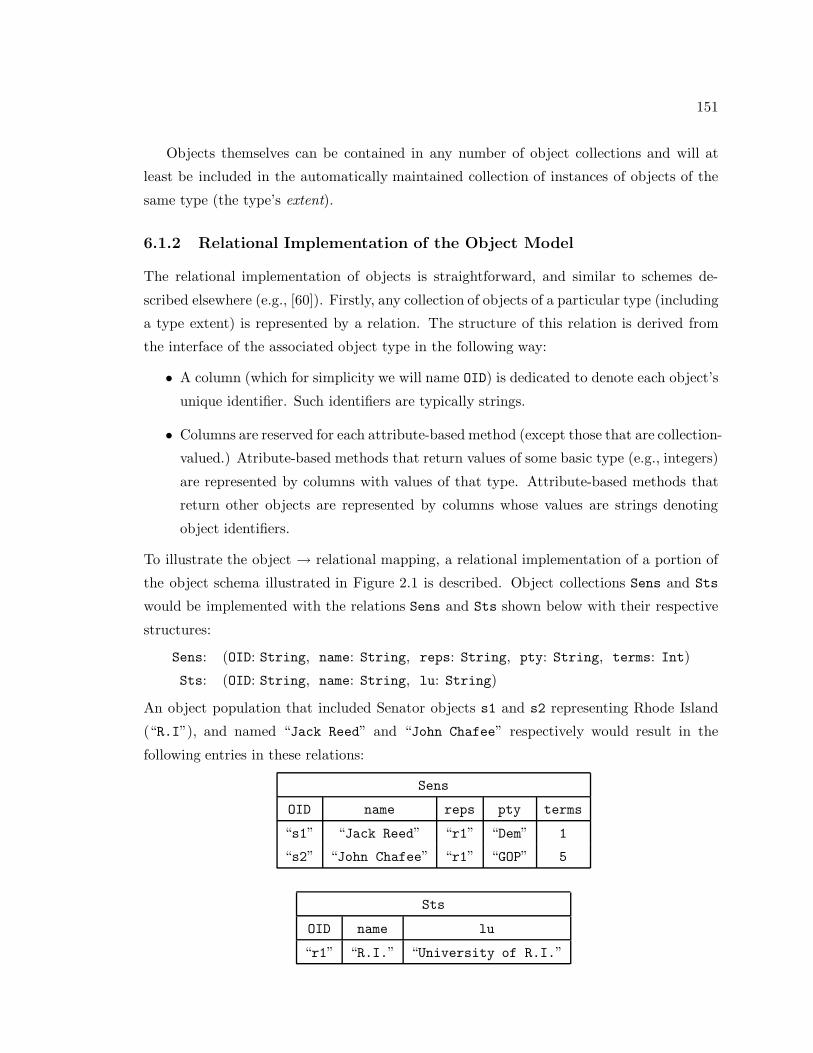
151
Objects themselves can be contained in any number of object collections and will at
least be included in the automatically maintained collection of instances of objects of the
same type (the type’s extent).
6.1.2 Relational Implementation of the Object Model
The relational implementation of objects is straightforward, and similar to schemes de-
scribed elsewhere (e.g., [60]). Firstly, any collection of objects of a particular type (including
a type extent) is represented by a relation. The structure of this relation is derived from
the interface of the associated object type in the following way:
• A column (which for simplicity we will name OID) is dedicated to denote each object’s
unique identifier. Such identifiers are typically strings.
• Columns are reserved for each attribute-based method (except those that are collection-
valued.) Atribute-based methods that return values of some basic type (e.g., integers)
are represented by columns with values of that type. Attribute-based methods that
return other objects are represented by columns whose values are strings denoting
object identifiers.
To illustrate the object → relational mapping, a relational implementation of a portion of
the object schema illustrated in Figure 2.1 is described. Object collections Sens and Sts
would be implemented with the relations Sens and Sts shown below with their respective
structures:
Sens: (OID: String, name: String, reps: String, pty: String, terms: Int)
Sts: (OID: String, name: String, lu: String)
An object population that included Senator objects s1 and s2 representing Rhode Island
(“R.I”), and named “Jack Reed” and “John Chafee” respectively would result in the
following entries in these relations:
Sens
OID name reps pty terms
“s1” “Jack Reed” “r1” “Dem” 1
“s2” “John Chafee” “r1” “GOP” 5
Sts
OID name lu
“r1” “R.I.” “University of R.I.”
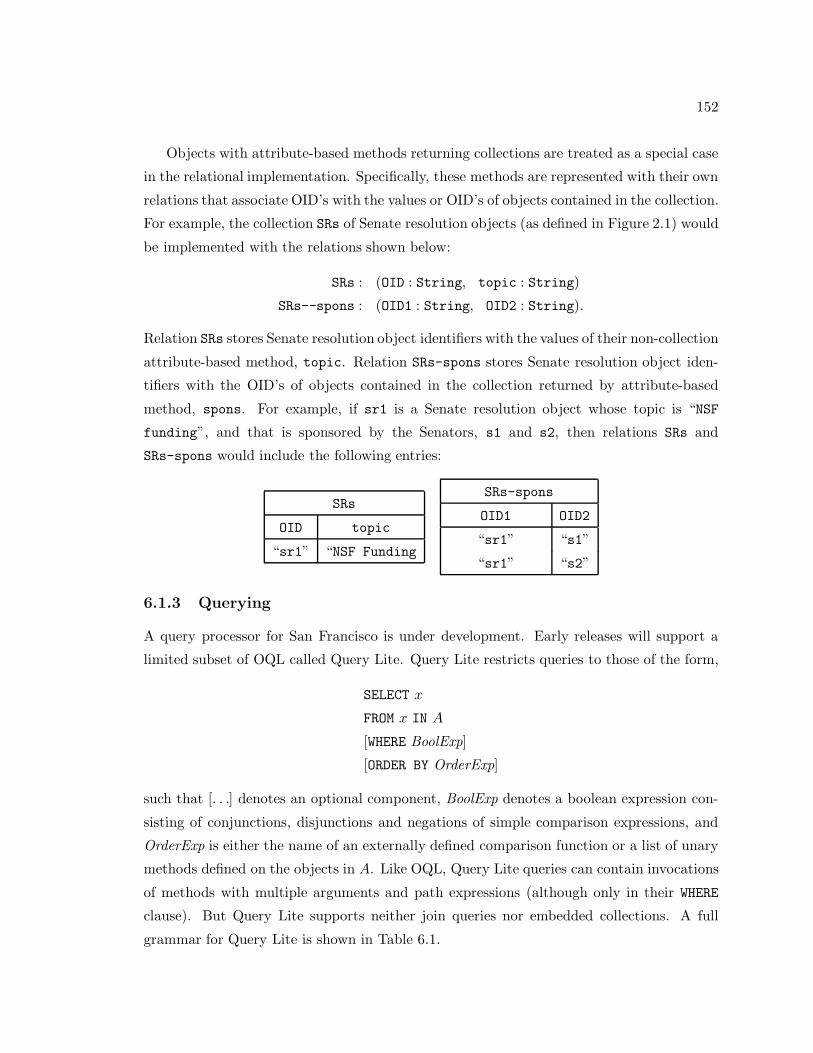
152
Objects with attribute-based methods returning collections are treated as a special case
in the relational implementation. Specifically, these methods are represented with their own
relations that associate OID’s with the values or OID’s of objects contained in the collection.
For example, the collection SRs of Senate resolution objects (as defined in Figure 2.1) would
be implemented with the relations shown below:
SRs : (OID : String, topic : String)
SRs--spons : (OID1 : String, OID2 : String).
Relation SRs stores Senate resolution object identifiers with the values of their non-collection
attribute-based method, topic. Relation SRs-spons stores Senate resolution object iden-
tifiers with the OID’s of objects contained in the collection returned by attribute-based
method, spons. For example, if sr1 is a Senate resolution object whose topic is “NSF
funding”, and that is sponsored by the Senators, s1 and s2, then relations SRs and
SRs-spons would include the following entries:
SRs
OID topic
“sr1” “NSF Funding
SRs-spons
OID1 OID2
“sr1” “s1”
“sr1” “s2”
6.1.3 Querying
A query processor for San Francisco is under development. Early releases will support a
limited subset of OQL called Query Lite. Query Lite restricts queries to those of the form,
SELECT x
FROM x IN A
[WHERE BoolExp]
[ORDER BY OrderExp]
such that [. . .] denotes an optional component, BoolExp denotes a boolean expression con-
sisting of conjunctions, disjunctions and negations of simple comparison expressions, and
OrderExp is either the name of an externally defined comparison function or a list of unary
methods defined on the objects in A. Like OQL, Query Lite queries can contain invocations
of methods with multiple arguments and path expressions (although only in their WHERE
clause). But Query Lite supports neither join queries nor embedded collections. A full
grammar for Query Lite is shown in Table 6.1.

153
6.1.4 Our Contribution
Our contribution was to build a query rewriter (using COKO-KOLA) that transforms Query
Lite queries with path expressions, into equivalent SQL queries over the underlying rela-
tional implementation.1 For example, the Query Lite query,
SELECT x
FROM x IN Sens
WHERE x.reps.name == ‘‘R.I.’’
gets rewritten by our rewriter into the SQL query,
SELECT x
FROM x IN Sens, y IN Sts
WHERE x.reps == y.OID AND y.name == ‘‘R.I.’’
(assuming the scheme for representing object collections as relations described in the pre-
vious section). This effort required that we (1) translate Query Lite queries with path
expressions into KOLA, (2) rewrite the KOLA path expression queries into KOLA join
queries, and (3) translate the KOLA join queries into SQL.2 The components required for
each of these tasks are illustrated in Figure 6.1. Sections 6.2, 6.3 and 6.4 present the designs
and implementations of these components.
6.2 Translating Query Lite Queries into KOLA
The simplicity of Query Lite makes a Query Lite → KOLA translator straightforward to
design. However, as the eventual goal of the San Francisco project is to support querying
in OQL, a sophisticated approach to translation is required. In this section, we describe the
reasoning behind our approach to translation, which accounts for an eventual migration to
OQL.1Because KOLA does not yet have support for lists, we only address Query Lite queries that do notcontain an ORDER BY clause.
2A fourth step to provide an object view over the relational data returned by the SQL queries is notconsidered here.

154
SQL Query
Query Lite Query
KOLA → SQLTranslator
DB2
Query Lite Query Processor
Query Lite → KOLATranslator
Query Rewriter
Figure 6.1: An Architecture for the Query Lite Query Rewriter

155
Constants, Variables and Path ExpressionsExp : c (c a non-Bool constant/global name)
| IDENT (an identifier denoting the name of a variable)
| Exp . IDENT| Exp . IDENT ( Exp , Exp , . . . , Exp )
Arithmetic Expressions| - ( Exp )| ABS ( Exp )| Exp + Exp| Exp - Exp| Exp * Exp| Exp / Exp| Exp MOD Exp
Query Expressions
Query :
SELECT x (Any variable name can be substituted for x)FROM x IN IDENT[WHERE BoolExp][ORDER BY OrdExp]
Boolean ExpressionsBoolExp : TRUE
| FALSE| Exp IS NULL| Exp IS NOT NULL| Exp == Exp| Exp != Exp| Exp < Exp| Exp > Exp| Exp <= Exp| Exp >= Exp| NOT ( BoolExp )| BoolExp AND BoolExp| BoolExp OR BoolExp
Ordering ExpressionsOrderExp : IDENT . IDENT, . . . , IDENT . IDENT Direction
| IDENT Direction
Direction : ASC | DESCTable 6.1: The Syntax of Query Lite

156
6.2.1 Translation Strategies
Translation from Query Lite into KOLA is straightforward. Given a Query Lite query e,
SELECT x
FROM x IN A
WHERE p (x),
KOLA equivalent of e (T JeK) is
iterate (T JpK, id) ! A.
This simplistic approach says that translation generates a KOLA query of the form,
f ! x,
such that x (the data component of the KOLA query) is generated from the expression in
the query’s FROM clause, and f (the function component of the KOLA query) is generated
from the expressions in the query’s SELECT and WHERE clauses.
We decided against this translation strategy because it does not generalize well to OQL,
the language that eventually will be used as the query language for San Francisco. Specifi-
cally, determining which parts of a query correspond to the data and function components
of the KOLA translation becomes blurred in the presence of nested queries and embedded
collections. Consider for example, the OQL query of Figure 6.2a, which finds all committees
with Republican members. This query invokes the method mems to return the embedded
collection of members of any given committee. The simplistic assumption that what ap-
pears in a query’s FROM clause is automatically the data component of a query is violated
here, as a collection of committee members can only be determined by applying a function
(mems) to a given committee. Therefore, the simplistic translation strategy that works for
Query Lite queries does not work for queries such as this.
An Alternative Strategy: The 1st Collection in a FROM Clause is Data
Consider the following alternative translation strategy: rather than designating all expres-
sions appearing a query’s FROM clause as data components, instead designate only the first
collection named in the FROM clause as a data component. Therefore, translation of the
query of Figure 6.2a would designate Coms as the only data component of the query, and
produce a KOLA query on Coms:
(iterate (eq ⊕ 〈pty ◦ π2, Kf (‘‘GOP’’)〉, π1) ◦ unnest (id, mems)) ! Coms.

157
SELECT DISTINCT xFROM x IN Coms, y IN x.memsWHERE y.pty == ‘‘GOP’’
a. A Query with a Path Expression (x.mems) in its FROM Clause
SELECT
SELECT y
FROM y IN x.memsWHERE y.terms > 5
FROM x IN ComsWHERE x.topic == ‘‘NSF’’
b. A Nested Query
Figure 6.2: OQL Queries that make Translation into KOLA Difficult
This query first pairs every committee with each of its members (unnest), and then deter-
mines which (committee, member) pairs satisfy the condition that member is a Republican
(iterate).
Once queries can be nested, this strategy also fails. Consider the nested query of Fig-
ure 6.2b which finds the senior members of committees in Coms that study the NSF. The
subquerySELECT y
FROM y IN x.mems
WHERE y.terms > 5
has the path expression, x.mems in its FROM clause. This expression is not a data component
and instead must be mapped to a function, even though it is the first expression in the FROM
clause. Therefore, this translation strategy must treat outer queries (queries that include
subqueries, which must get translated to function invocations) differently from inner queries
(queries that are subexpressions of outer queries, which must get translated into functions).
Our Strategy: Everything Generates a Function
The solution we take is to designate all parts of the query as function components. This
approach to translation simplifies the design of the translator greatly as it removes the
need to analyze each subexpression to see if it constitutes data or function. However, the
consequence of this design decision is that translation returns KOLA expressions that are
not intuitive. This problem is addressed after translation by a normalization (defined in
COKO) to rewrite translated queries into more intuitive forms.

158
SELECT xFROM x IN SensWHERE x.terms > 5
a. A Query Lite Query
(iterate (gt ⊕ 〈terms ◦ π2, Kf (5)〉, π2) ◦unnest (id, Kf (Sens)) ◦single) ! NULL
b. Translation Into KOLA
iterate (gt ⊕ 〈id, Kf (5)〉 ⊕ terms, id) ! Sensc. After Normalization
Figure 6.3: A Query Lite Query (a), its Translation (b) and its Normalization (c)
Figures 6.3a and 6.3b show a simple Query Lite query (that finds all Senators who
have served more than 5 terms) and the result of translating this query according to this
strategy. Note that translation produces a function that gets invoked on NULL. NULL is an
arbitrary argument to this function; in fact the function would return the same result no
matter what was its argument (i.e., the function generated by the translator is a constant
function). This translation strategy makes the result of translation counterintuitive, as the
query that is produced does not get invoked on one or more collections, but on a constant
that does not even figure in the final result.
The result of translation shown in 6.3b is not as intuitive a translation as the equivalent
KOLA query shown in Figure 6.3c, which simply filters Senators in Sens who have served
more than 5 terms. However, the KOLA expression of Figures 6.3b has the same semantics
as the initial Query Lite query, as is demonstrated by the reduction below:
(iterate (gt ⊕ 〈terms ◦ π2, Kf (5)〉, π2) ◦unnest (id, Kf (Sens)) ◦ single) ! NULL
1→ iterate (gt ⊕ 〈terms ◦ π2, Kf (5)〉, π2) !
(unnest (id, Kf (Sens)) ! (single ! NULL))2→ iterate (gt ⊕ 〈terms ◦ π2, Kf (5)〉, π2) ! (unnest (id, Kf (Sens)) ! {|NULL|})3→ iterate (gt ⊕ 〈terms ◦ π2, Kf (5)〉, π2) !
({|(id ! [x, s])ij | xi ∈ {|NULL|}, sj ∈ (Kf (Sens) ! x)|})4→ iterate (gt ⊕ 〈terms ◦ π2, Kf (5)〉, π2) ! ({|[x, s]ij | xi ∈ {|NULL|}, sj ∈ Sens|}

159
5→ iterate (gt ⊕ 〈terms ◦ π2, Kf (5)〉, π2) ! ({|[NULL, s]j | sj ∈ Sens|}6→ {|(π2 ! [NULL, s])j | sj ∈ Sens, (gt ⊕ 〈terms ◦ π2, Kf (5)〉) ? [NULL, s]|}7→ {|(π2 ! [NULL, s])j | sj ∈ Sens, gt ? (〈terms ◦ π2, Kf (5)〉 ! [NULL, s])|}8→ {|sj | sj ∈ Sens, gt ? [(terms ◦ π2) ! [NULL, s], Kf (5) ! [NULL, s]]|}9→ {|sj | sj ∈ Sens, gt ? [terms ! (π2 ! [NULL, s]), Kf (5) ! [NULL, s]]|}10→ {|sj | sj ∈ Sens, gt ? [terms ! s, Kf (5) ! [NULL, s]]|}11→ {|sj | sj ∈ Sens, gt ? [s.terms, Kf (5)]|}12→ {|sj | sj ∈ Sens, s.terms > 5|}
Step 1 of this reduction follows from the definition of ◦. Step 2 follows from the definition
of single. Step 3 follows from the definition of unnest. Step 4 follows from the definitions
of id and Kf . Step 5 follows from the fact that xi is being drawn from a singleton set. Step
6 follows from the definition of iterate. Step 7 follows from the definition of ⊕. Step 8
follows from the definition of 〈 〉. Step 9 follows from the definition of ◦. Step 10 follows
from the definition of π2. Step 11 follows from the definition of function attribute primitives
and Kf . Step 12 follows from the definition of gt.
Our approach to translation is similar to how Query Lite or OQL queries would be
given a denotational semantics. Because arbitrary Query Lite and OQL expressions can
have occurences of free variables (e.g., x in “x > 5”), the semantics of such expressions is
dependent on an environment that defines what is referred to by the free variables appearing
within the expression. More precisely, an environment is a list of (variable, value) pairs
((v1, d1), (v2, d2), . . . , (vn, dn))
providing the bindings of all free variables, v1, . . . , vn appearing in a given expression. (If
an environment ρ gives bindings to every free variable in an expression, e, we say that e
is well-formed with regard to to ρ.) The denotational semantics of a Query Lite or OQL
expression, e is a function (Eval JeK) that maps all environments for which it is well-formed
to values. For example,
Eval Jx > 5K ρ
is true if ρ = ((x, 6)) but false if ρ = ((x, 4)). Queries that do not appear as subexpressions
of other queries will have no free variables, and therefore are well-formed with regard to
the empty environment, (). The denotational semantics of these expressions are constant
functions.

160
The idea behind this translation strategy is to map every expression e to the KOLA
function T JeK whose operational semantics coincides with e’s denotational semantics. More
precisely, if e is well-formed with respect to some environment,
ρ = ((v1, d1), (v2, d2), . . . , (vn, dn)),
then T JeK is a KOLA function satisfying the constraint that
T JeK ! (ρ) = Eval JeK ρ
such that ρ is the KOLA nested pair representation of environment ρ,
[. . .[d1, d2], . . .dn].3
Queries that are well-formed with regard to the empty environment get mapped to constant
KOLA functions. The choice of NULL as an argument to these functions can be thought of
as reflecting how KOLA represents the empty environment (i.e., () = NULL).
6.2.2 T: The Query Lite → KOLA Translation Function Described
We have defined a translator from a set-and-bag-based subset of OQL to KOLA. This subset
of OQL is a superset of Query Lite. The part of the translator that processes Query Lite
queries is described here. (The full OQL translator is described and proven correct in [17].4)
The translation of a Query Lite query q, is
T JqK ! NULL
such that T JqK is as defined in Table 6.2. Below we examine this translation function,
defined over all Query Lite queries and expressions.
Translating Constants
All non-Bool constants (e.g., −3, 5.322, ‘‘Hello World’’, NULL, . . .) are translated into
constant functions (Kf (−3), Kf (5.32), Kf (‘‘Hello World’’), Kf (NULL), . . .). (Bool
constants are translated into constant predicates Kp (TRUE) and Kp (FALSE).)3A boolean expression b would similarly be mapped to KOLA predicate, T JbK such that
T JbK ? (ρ) = Eval JbK ρ.
4In fact, an older translator that translates a set-based (as opposed to a set-and-bag based) subset ofOQL is presented and proven correct in a technical report [17]. The correctness proof (by structuralinduction) is nonetheless highly suggestive of what the correctness proof for this version of the translatorwill involve. The updated correctness proof is future work.

161
Constants, Variables and Path ExpressionsT JcK = Kf (c) (c a non-Bool constant/global name)
T JV0K = π2
T JViK = T JVi−1K ◦ π1 (for i > 0)
T JExp . IDENTK = IDENT ◦ T JExpKT JExp . IDENT (Exp1, Exp2, . . . , Expn)K =IDENT ◦ 〈T JExpK, 〈〈 . . . 〈T JExp1K, T JExp2K〉, . . . 〉, T JExpnK〉〉
Arithmetic ExpressionsT J− (Exp)K = Cf (mul, −1) ◦ T JExpK
T JABS (Exp)K = abs ◦ T JExpKT JExp0 + Exp1K = add ◦ 〈T JExp0K, T JExp1K〉T JExp0 - Exp1K = sub ◦ 〈T JExp0K, T JExp1K〉T JExp0 * Exp1K = mul ◦ 〈T JExp0K, T JExp1K〉T JExp0 / Exp1K = div ◦ 〈T JExp0K, T JExp1K〉
T JExp0 MOD Exp1K = mod ◦ 〈T JExp0K, T JExp1K〉Query Expressions
T
uv SELECT xFROM x IN IDENTWHERE BoolExp
}~ =iterate (T JBoolExpK, π2) ◦unnest (id, Kf (IDENT)) ◦single
Boolean ExpressionsT JTRUEK = Kp (TRUE)
T JFALSEK = Kp (FALSE)
T JExp IS NULLK = isnull ⊕ T JExpKT JExp IS NOT NULLK = isnotnull ⊕ T JExpK
T JExp0 == Exp1K = eq ⊕ 〈T JExp0K, T JExp1K〉T JExp0 != Exp1K = neq ⊕ 〈T JExp0K, T JExp1K〉T JExp0 < Exp1K = lt ⊕ 〈T JExp0K, T JExp1K〉T JExp0 > Exp1K = gt ⊕ 〈T JExp0K, T JExp1K〉
T JExp0 <= Exp1K = leq ⊕ 〈T JExp0K, T JExp1K〉T JExp0 >= Exp1K = geq ⊕ 〈T JExp0K, T JExp1K〉T JNOT (BoolExp)K = ∼ (T JBoolExpK)
T JBoolExp0 AND BoolExp1K = T JBoolExp0K & T JBoolExp1KT JBoolExp0 OR BoolExp1K = T JBoolExp0K | T JBoolExp1K
Table 6.2: T: The Query Lite → KOLA Translation Function

162
Translating Variables
The translation of variables is perhaps the most complex aspect of translation. Conceptu-
ally, variable translation works from a preprocessed version of the query in which all variable
references are replaced by deBruijn variables [30]. A deBruijn variable is a variable index
(Vi for i ≥ 0) that indicates the position of a variable reference relative to its declaration.
(Higher values of i indicate a greater “distance” between reference and declaration. V0
always refers to the most “recently” declared variable.)
The preprocessing step that converts variable references into deBruijn variables must
first associate every referenced variable with its declaration. Variable declarations typically
occur in a query’s FROM clause, as in “x IN COLL”, which declares variable x to range over
the elements of collection COLL. In OQL, variable declarations can also occur in a query’s
WHERE clause if it contains a quantifier expression, as in
EXISTS x IN COLL: p (x)
which also declares variable x to range over the elements of collection COLL.
The algorithm followed during this preprocessing step visits each subexpression of a
given query expression’s FROM, SELECT and WHERE clauses in turn. Each subexpression
is associated with a scope list which is a list of variables that can be referenced by the
subexpression.5 Scope lists of subexpressions are propagated and amended during each
step of the expression traversal. That is, the visit of a subexpression will accept the scope
list associated with a previously visited subexpression (its incoming scope list). If the
subexpression declares a new variable, this variables is appended to the incoming scope list
to produce a scope list for subexpressions still to be visited (its outgoing scope list).
The algorithm is described below with respect to the generic OQL query of Figure 6.4.6
In this figure, Es, Ew, and Ei, . . . , Em (0 ≤ i ≤ m) are OQL subexpressions that potentially
include free occurences of variables. For this example, it is assumed that this query has
(x0, . . . , xi−1)
as its incoming scope list. (If the query is not a subexpression of another query, then its
incoming scope list is (). That is, i = 0.)
The subexpressions of this query are visited and processed as follows:5The variables in a subexpression’s scope list are those that must be bound by any environment for whichthat subexpression is well-formed.
6The algorithm is described in terms of an OQL query rather than a Query Lite query because everyQuery Lite query declares exactly one variable, making preprocessing trivial.

163
SELECT Es
FROM xi IN Ei, . . . , xm IN Em
WHERE Ew
Figure 6.4: A Prototypical OQL Query
1. for each FROM subexpression: Ek (i ≤ k ≤ m):
• Ek’s incoming scope list is (x0, . . . , xk−1).
• conversion into deBruijn notation replaces each xj appearing in Ek with Vk−j−1.
• Ek’s outgoing scope list is (x0, . . . , xk). (That is, xk is appended to the incoming
scope list.)
2. for SELECT subexpression, Es and WHERE subexpression Ew:
• Es’s and Ew’s incoming scope lists are both (x0, . . . , xm).
• conversion into deBruijn notation replaces each xj in Es or Ew with Vm−j.
To illustrate the algorithm, we trace its effects on the OQL query of Figure 6.2b that is
nested in its SELECT clause. Assume that the outer query does not appear as a subexpression
of another query (i.e., the outer query is defined with respect to the empty environment,
()). The algorithm visits subexpressions of this query in the following order:
1. “x IN Kf (Coms)”:
1’s Incoming Scope List: ()
1’s Outgoing Scope List: (x)
Expression 1’s outgoing scope list is the result of appending its declared variable x to
its incoming scope list, ().
2. “SELECT y FROM y IN x.mems WHERE y.terms > 5”:
2’s Incoming Scope List: (x)
(a) “y IN x.mems” (in inner query’s FROM clause):
2a’s Incoming Scope List: (x)
2a’s deBruijn Conversion: variable reference x is replaced by V0
2a’s Outgoing Scope List: (x, y)

164
SELECT
SELECT V0
FROM y IN V0.memsWHERE V0.terms > 5
FROM x IN ComsWHERE V0.topic == ‘‘NSF’’
Figure 6.5: The Query of Figure 6.2b After deBruijn Conversion
Expression 2a’s outgoing scope list is the result of appending its declared variable
y to its incoming scope list, (x).
(b) “SELECT y” (in inner query):
2b’s Incoming Scope List: (x, y)
2b’s deBruijn Conversion: variable reference y is replaced by V0
Variable y was the most “recently” declared variable in the incoming scope list
and hence its reference is replaced by V0. Had this reference instead been to x,
it would have been replaced by V1.
(c) “WHERE y.terms > 5” (in inner query):
2c’s Incoming Scope List: (x, y)
2c’s deBruijn Conversion: variable reference y is replaced by V0
After preprocessing of this query is completed, we are left with the query of Figure 6.5.
Note that the relative referencing of deBruijn notation means that the same deBruijn index
can refer to multiple variables within a single query. In the query of Figure 6.5, deBruijn
variable V0 refers to a committee in Coms in the WHERE clause of the outer query and the
FROM clause of the inner query, but refers to a committee member in the SELECT and WHERE
clauses of the inner query.
The translation of a deBruijn variable (Vi) into KOLA is defined as follows:
• T JV0K = π2, and
• T JViK (for i > 0) = T JVi−1K ◦ π1
The result of translation then, is a function that can be invoked on the KOLA representation
(ρ) of the environment (ρ) associated with the translated variable. When invoked on this
representation, the value bound to the variable in the environment is returned. For example,
suppose that variable reference x is associated with the incoming scope list,
(w, x, y, z)
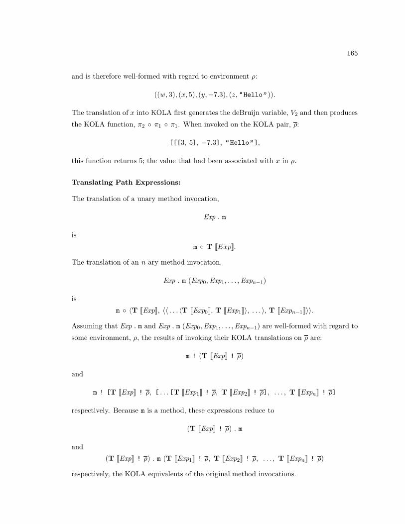
165
and is therefore well-formed with regard to environment ρ:
((w, 3), (x, 5), (y,−7.3), (z, ‘‘Hello’’)).
The translation of x into KOLA first generates the deBruijn variable, V2 and then produces
the KOLA function, π2 ◦ π1 ◦ π1. When invoked on the KOLA pair, ρ:
[[[3, 5], −7.3], ‘‘Hello’’],
this function returns 5; the value that had been associated with x in ρ.
Translating Path Expressions:
The translation of a unary method invocation,
Exp . m
is
m ◦ T JExpK.The translation of an n-ary method invocation,
Exp . m (Exp0, Exp1, . . . , Expn−1)
is
m ◦ 〈T JExpK, 〈〈 . . . 〈T JExp0K, T JExp1K〉, . . . 〉, T JExpn−1K〉〉.Assuming that Exp . m and Exp . m (Exp0, Exp1, . . . , Expn−1) are well-formed with regard to
some environment, ρ, the results of invoking their KOLA translations on ρ are:
m ! (T JExpK ! ρ)
and
m ! [T JExpK ! ρ, [ . . .[T JExp1K ! ρ, T JExp2K ! ρ], . . . , T JExpnK ! ρ]
respectively. Because m is a method, these expressions reduce to
(T JExpK ! ρ) . m
and
(T JExpK ! ρ) . m (T JExp1K ! ρ, T JExp2K ! ρ, . . . , T JExpnK ! ρ)
respectively, the KOLA equivalents of the original method invocations.

166
Translating Arithmetic Expressions:
Every arithmetic operator (e.g., ‘+’) has a corresponding KOLA primitive (e.g., add). The
translation of any arithmetic subexpression,
Exp0 ArithOp Exp1,
is the KOLA function,
ArithOp ◦ 〈T JExp0K, T JExp1K〉such that ArithOp is the KOLA primitive corresponding to ArithOp.
Translating Query Expressions:
For any OQL or Query Lite query, q:
T
uwwvSELECT Es
FROM x0 IN E0, . . . , xn IN En
WHERE Ew
}��~=
iterate (T JE ′wK, T JE ′
sK) ◦unnest (id, T JE ′
nK) ◦ . . . ◦ unnest (id, T JE ′0K) ◦
single
such that each E ′i (for i ∈ {0, . . . , n, s, w}) is equivalent to Ei but for the replacement of all
variable references with their deBruijn equivalents. The translation of a Query Lite query
(for which n = 0) follows from the more general translation of OQL queries shown here.
That the translation of query expressions preserves semantics is demonstrated below.
Suppose that q (above) is well-formed with regard to some environment, ρ. Then T JqK ! (ρ)
reduces as follows:
1. Function single is invoked to create the singleton bag, {|ρ|}).
2. Successive invocations of unnest (id, E ′0), . . ., unnest (id, T JE ′
nK) generate the
collection,
{|[. . .[[ρ, e0], e1], . . . en] |e0 ∈ (T JE ′
0K ! (ρ)),
e1 ∈ (T JE ′1K ! ([ρ, e0])),
. . . ,
em ∈ (T JE ′nK ! ([. . .[[ρ, e0], e1], . . . , en−1]))|}.

167
The result above is a bag of KOLA pairs,
[. . .[[ρ, e0], e1], . . . en]
such that ei (0 ≤ i ≤ n) is an element of the collection denoted by Ei with regard to
ρ supplemented with pairs,
((x0, e0), . . . , (xi−1, ei−1)).
Put another way, this result is an (n + 1)-way cartesian product of the collections
denoted by E0, . . . , En with regard to the environments derived from ρ, and from
elements of preceeding collections.
3. Query iterate (T JE ′wK, T JE ′
sK) is invoked on the result of 2, thereby applying the
expression in the original query’s SELECT clause (T JE ′sK) to every tuple produced in
2 that satisfies the query’s WHERE clause (T JE ′wK).
Translating Boolean Expressions:
The translation of Boolean expressions is straightforward, resembling the translation of
non-Boolean expressions but with combination (⊕) replacing composition (◦).
6.2.3 Sample Traces of Translation
In this section, we trace the application of the translation function on two queries: the
Query Lite query of Figure 6.3 and the OQL query of Figure 6.2b. The result of translating
the Query Lite query is shown in Figure 6.3b. The result of translating the OQL query and
also that of Figure 6.2a are shown in Figure 6.6.
Tracing the Translation of the Query Lite Query of Figure 6.3
The translation of the Query Lite query of Figure 6.3 first converts all variable references
to deBruijn variables, producing the query,
SELECT V0
FROM x IN Sens
WHERE V0.terms > 5.
Translation then proceeds as follows:
T JSELECT V0 FROM x IN Sens WHERE V0.terms > 5K

168
a:(set ◦ iterate (eq ⊕ 〈pty ◦ π2, Kf (‘‘GOP’’)〉, π2 ◦ π1) ◦unnest (id, mems ◦ π2) ◦ unnest (id, Kf (Coms)) ◦ single) ! NULL
b:(iterate (eq ⊕ 〈topic ◦ π2, Kf (‘‘NSF’’)〉, f) ◦unnest (id, Kf (Coms)) ◦ single) ! NULL
such that f =(iterate (gt ⊕ 〈terms ◦ π2, Kf (5)〉, π2) ◦unnest (id, mems ◦ π2) ◦ single)
Figure 6.6: Results of Translating the OQL queries of Figure 6.2
= iterate (T JV0.terms > 5K, T JV0K) ◦ unnest (id, T JSensK) ◦ single
= iterate (T JV0.terms > 5K, π2) ◦ unnest (id, Kf (Sens)) ◦ single
= iterate (gt ⊕ 〈T JV0.termsK, T J5K〉, π2) ◦ unnest (id, Kf (Sens)) ◦ single
= iterate (gt ⊕ 〈terms ◦ T JV0K, Kf (5)〉, π2) ◦ unnest (id, Kf (Sens)) ◦ single
= iterate (gt ⊕ 〈terms ◦ π2, Kf (5)〉, π2) ◦ unnest (id, Kf (Sens)) ◦ single
Tracing the Translation of the OQL Query of Figure 6.2b
The translation of the OQL query of Figure 6.2b first converts all variable references to
deBruijn variables, producing the query of Figure 6.5. Translation then proceeds as follows:
T
uwwwwwwwvSELECT
SELECT V0
FROM y IN V0.mems
WHERE V0.terms > 5
FROM x IN Coms
WHERE V0.topic == ‘‘NSF’’
}�������~
=iterate (T JV0.topic == ‘‘NSF’’K, f) ◦unnest (id, T JComsK) ◦ single
s.t. f = T
uwwvSELECT V0
FROM y IN V0.mems
WHERE V0.terms > 5
}��~

169
=iterate (T JV0.topic == ‘‘NSF’’K, f) ◦unnest (id, T JComsK) ◦ single
s.t. f =iterate (T JV0.terms > 5K, T JV0K) ◦unnest (id, T JV0.memsK) ◦ single
=iterate (eq ⊕ 〈T JV0.topicK, T J‘‘NSF’’K〉, f) ◦unnest (id, T JComsK) ◦ single
s.t. f =iterate (gt ⊕ 〈T JV0.termsK, T J5K〉, T JV0K) ◦unnest (id, T JV0.memsK) ◦ single
=iterate (eq ⊕ 〈T JV0.topicK, Kf (‘‘NSF’’)〉, f) ◦unnest (id, Kf (Coms)) ◦ single
s.t. f =iterate (gt ⊕ 〈T JV0.termsK, Kf (5)〉, T JV0K) ◦unnest (id, T JV0.memsK) ◦ single
=iterate (eq ⊕ 〈topic ◦ T JV0K, Kf (‘‘NSF’’)〉, f) ◦unnest (id, Kf (Coms)) ◦ single
s.t. f =iterate (gt ⊕ 〈terms ◦ T JV0K, Kf (5)〉, T JV0K) ◦unnest (id, mems ◦ T JV0K) ◦ single
=iterate (eq ⊕ 〈topic ◦ π2, Kf (‘‘NSF’’)〉, f) ◦unnest (id, Kf (Coms)) ◦ single
s.t. f =iterate (gt ⊕ 〈terms ◦ π2, Kf (5)〉, π2) ◦unnest (id, mems ◦ π2) ◦ single
The bravehearted can now follow the reduction of this function when invoked on NULL, to
confirm that translation has preserved query semantics.

170
(iterate (eq ⊕ 〈topic ◦ π2, Kf (‘‘NSF’’)〉, f) ◦unnest (id, Kf (Coms)) ◦ single) ! NULL
s.t. f =iterate (gt ⊕ 〈terms ◦ π2, Kf (5)〉, π2) ◦unnest (id, mems ◦ π2) ◦ single
=iterate (eq ⊕ 〈topic ◦ π2, Kf (‘‘NSF’’)〉, f) !
(unnest (id, Kf (Coms)) ! (single ! NULL))
s.t. f =iterate (gt ⊕ 〈terms ◦ π2, Kf (5)〉, π2) ◦unnest (id, mems ◦ π2) ◦ single
=iterate (eq ⊕ 〈topic ◦ π2, Kf (‘‘NSF’’)〉, f) !
(unnest (id, Kf (Coms)) ! {|NULL|})
s.t. f =iterate (gt ⊕ 〈terms ◦ π2, Kf (5)〉, π2) ◦unnest (id, mems ◦ π2) ◦ single
= iterate (eq ⊕ 〈topic ◦ π2, Kf (‘‘NSF’’)〉, f) ! {|([NULL, c])i | ci ∈ Coms|}
s.t. f =iterate (gt ⊕ 〈terms ◦ π2, Kf (5)〉, π2) ◦unnest (id, mems ◦ π2) ◦ single
= {|(f ! [NULL, c])i | ci ∈ Coms, (eq ⊕ 〈topic ◦ π2, Kf (‘‘NSF’’)〉) ? [NULL, c]|}
s.t. f =iterate (gt ⊕ 〈terms ◦ π2, Kf (5)〉, π2) ◦unnest (id, mems ◦ π2) ◦ single
= {|(f ! [NULL, c])i | ci ∈ Coms, eq ? [c.topic, ‘‘NSF’’]|}
s.t. f =iterate (gt ⊕ 〈terms ◦ π2, Kf (5)〉, π2) ◦unnest (id, mems ◦ π2) ◦ single
.

171
The invocation of f on [NULL, c] then reduces as follows:
f ! [NULL, c] =(iterate (gt ⊕ 〈terms ◦ π2, Kf (5)〉, π2) ◦unnest (id, mems ◦ π2) ◦ single) ! [NULL, c]
=iterate (gt ⊕ 〈terms ◦ π2, Kf (5)〉, π2) !
(unnest (id, mems ◦ π2) ! (single ! [NULL, c]))
=iterate (gt ⊕ 〈terms ◦ π2, Kf (5)〉, π2) !
(unnest (id, mems ◦ π2) ! {|[NULL, c]|})
=iterate (gt ⊕ 〈terms ◦ π2, Kf (5)〉, π2) !
{|([[NULL, c], m])j |mj ∈ ((mems ◦ π2) ! [NULL, c])|}
=iterate (gt ⊕ 〈terms ◦ π2, Kf (5)〉, π2) !
{|([[NULL, c], m])j |mj ∈ c.mems|}
={|(π2 ! [[NULL, c], m])j |
mj ∈ c.mems, (gt ⊕ 〈terms ◦ π2, Kf (5)〉) ? [[NULL, c], m]|}
= {|mj |mj ∈ c.mems, m.terms > 5|}
The result of this reduction then is
{|{|mj |mj ∈ c.mems, m.terms > 5|}i | ci ∈ Coms, c.topic == ‘‘NSF’’|}
which is a nested bag of committee members for committees whose topic concerns the NSF
(i.e., the result specified by the original OQL query).
6.2.4 Translator Implementation
The translator described above was implemented with the Ox compiler generator tool [8].
Ox is an attribute-grammar [3] based compiler tool in the spirit of Lex and Yacc [55].
Lex is a tool for generating lexical scanners and Yacc is a tool for generating parsers.
Lex specifications designate a set of tokens (or terminal symbols) and associate regular
expressions with each. The generated scanner maps text to tokens according to these
specifications. Yacc specifications are context-free grammars consisting of non-terminals
and tokens. The generated parser finds parse trees for strings according to the grammar
specification, and can also invoke semantic actions based on the parse.
Ox generalizes the operation of Yacc in the same manner that attribute grammars
generalize context-free grammars. Ox specifications are Lex and Yacc specifications that

172
are augmented with definitions of attributes that are either synthesized (passed up the
parse tree) or inherited (passed down the parse tree). Ox then uses these specifications to
generate a program that constructs and decorates attributed parse trees. Ox facilitates the
generation of compilers by making it possible to succinctly specify actions for those aspects
of compiler generation for which Yacc falls short, such as type checking, code generation
and so on.
To use Ox for the OQL/Query Lite → KOLA translator, we used a grammar augmented
with attributes denoting:
• functions and predicates: As described earlier, our translator returns a function or
predicate as the result of translating every expression. The function or predicate for
any given expression is constructed from the functions and predicates of its subex-
pressions, as the translation function T of Table 6.2 illustrates. Therefore, func and
pred are synthesized attributes of all expression non-terminals.
• incoming and outgoing scope lists: Scope lists are propagated from subexpression
to subexpression; one subexpression’s outgoing scope list becomes the next visited
subexpression’s incoming scope list. Therefore, insl is an inherited attribute denoting
the incoming scope list of all expressions, and outsl is a synthesized attribute denoting
the outgoing scope list.
6.3 Query Rewriting
This section presents COKO transformations that rewrite KOLA translations of Query Lite
queries into a form that can be translated into SQL. Section 6.3.1 presents a library of gen-
eral purpose COKO transformations used by these transformations. Section 6.3.2 presents a
specialized COKO transformation that normalizes KOLA queries resulting from translation
into a more intuitive form.7 Section 6.3.3 presents a specialized COKO transformation that
rewrites the resulting normalized KOLA queries into equivalent KOLA queries that can be
translated into SQL.
6.3.1 A Library of General-Purpose COKO Transformations
Many of the transformations defined for the Query Lite rewrites serve a more general-
purpose as normalization or simplification transformations. Whereas normalizations rewrite7These normalizations are strictly unnecessary, but make it easier to implement rewrites proposed in theliterature in terms of the more intuitive expressions of queries.

173
TRANSFORMATION LBCompUSESsft: f ◦ (g ◦ h) −→ (f ◦ g) ◦ h
BEGINBU {sft →
{GIVEN f ◦ F DO LBComp (f);LBComp}
}END
Figure 6.7: Transformation LBComp
expressions into structurally characterizable forms, simplifications make expressions “smaller”
by removing redundancies or trivial subexpressions. In this section, we describe the library
of general-purpose transformations defined for this task.
Normalizations
Left-Bushy Compositions LBComp (shown in Figure 6.7) is a normalization transfor-
mation that gets fired on KOLA functions. If the function is of the form,
f0 ◦ f1 ◦ . . . ◦ fn
(with compositions associated in any way), this transformation returns the equivalent func-
tion in “left-bushy” form:
(. . . (f0 ◦ f1) ◦ . . . ◦ fn).
The transformation of Figure 6.7 is similar to transformation LBComp from Figure 4.10
(Chapter 4). The firing algorithms and rewrite rules for these transformations are identical,
but for the use LBComp’s use of a composition former where LBConj has a conjunction former,
and LBComp’s use of function variables where LBConj has predicate variables.
Left-Bushy Joins Transformation LBJoin (Figure 6.8) gets applied to KOLA join queries
that have subqueries that are also joins. The effect of this transformation is to rewrite a
query with multiple applications of KOLA’s join operator into left-bushy form. For exam-
ple, the bushy join,
join (p, f) ! [join (q, g) ! [A1, A2], join (r, h) ! [B1, B2]]
gets transformed into the left-bushy join,
join (p′, f ′) ! [join (Kp (true), id) ! [join (Kp (true), id) ! [A1, A2], B1], B2]

174
such that p′ is derived from p, q and r, f ′ is derived from f , g and h, and join (Kp (true), id)
is the KOLA equivalent of the Cartesian product operator.
LBJoin is defined in terms of auxiliary transformations LBJAux (shown in Figure 6.8),
LBJAux2 (shown in Figure 6.9) and PullFP (also shown in Figure 6.9). Its firing algorithm
does the following:
1. Step 1: The auxiliary transformation, PullFP, “pulls up” all data functions and predi-
cates from join subqueries into the outermost join. The effect of this step is to return
a new join query that has the same structure as the initial query, but with all but
the outermost join replaced with Cartesian products.
2. Step 2: In this step, the large data predicate and data function now contained in the
outermost join (i.e., p and f in join (p, f)) are simplified by calls to COKO transfor-
mations SimpPred and SimpFunc respectively. (These simplification transformations
are presented in the next section.)
3. Step 3: This step performs all the necessary reassociations of joins to make the ex-
pression left-bushy. Transformation LBJAux (shown in Figure 6.8) invokes LBJAux2
in bottom-up fashion. LBJAux2 reassociates individual join by firing rule sft, which
rewrites a right associated join to a left associated join by combining (composing)
the data function (data predicate) instantiating the outermost join with shr (shift
right).
4. Step 4: This step repeats the action of Step 2 to simplify the data function and data
predicate in the outermost join operator.
Simplifications
Function Simplification Figure 6.10 shows the COKO transformation SimpFunc and its
auxiliary transformations. These transformations simplify functions built from the KOLA
primitives, id, π1, π2, shr and shl, and the KOLA formers, ◦, 〈 〉 and Kf . SimpFunc first
normalizes functions so that all composition chains (i.e., functions of the form f0 ◦ . . . ◦ fn)
contained as subfunctions are made left-bushy (via a call to LBComp). Next, auxiliary
transformation SFAux is invoked. This transformation applies the simplifying identities of
transformations BSAux1 and BSAux2 in a bottom-up fashion. If none of the rules in these
latter transformations fires on a given subquery, rules sft and dis are successively fired to
see if reassociation of compositions or distribution of compositions over function pairs (〈 〉)

175
TRANSFORMATION LBJoin-- Convert n-ary join to left-bushy joinUSEScu: iterate (Kf (true), id) ! A −→ A,SimpPred,SimpFunc,PullFP,LBJAux
BEGIN-- Step 1: Pull Up Data Predicates and Data FunctionsPullFP;
-- Step 2: Simplify Top-Most Predicate and Data Function{GIVEN iterate (p, f) ! A DO {SimpPred (p); SimpFunc (f); cu}} ||
{GIVEN join (p, f) ! O DO {SimpPred (p); SimpFunc (f)}};
-- Step 3: ReorderLBJAux;
-- Step 4: Simplify{GIVEN iterate (p, f) ! A DO {SimpPred (p); SimpFunc (f); cu}} ||
{GIVEN join (p, f) ! O DO {SimpPred (p); SimpFunc (f)}}END
TRANSFORMATION LBJAux-- Helps to Convert n-ary join to left-bushy joinUSESLBJAux2
BEGINBU {GIVEN join ( P, F) ! O DO LBJAux2}
END
Figure 6.8: Transformations LBJoin and LBJAux

176
TRANSFORMATION LBJAux2-- Helps to Convert n-ary join to left-bushy joinUSESpull1: join (p, f) ! [join (q, g) ! [A1, A2], B] −→
join ((q ⊕ π1) & (p ⊕ 〈g ◦ π1, π2〉), f ◦ 〈g ◦ π1, π2〉) ![join (Kf (true), id) ! [A1, A2], B],
pull2: join (p, f) ! [A, join (q, g) ! [B1, B2]] −→join ((q ⊕ π2) & (p ⊕ 〈π1, g ◦ π2〉), f ◦ 〈π1, g ◦ π2〉) ![A, join (Kf (true), id) ! [B1, B2]],
sft: join (p, f) ! [A, join (Kf (true), id) ! [B1, B2]] −→join (p ⊕ shr, f ◦ shr) ! [join (Kf (true), id) ! [A, B1], B2],
SimpFunc,SimpPred
BEGINpull1 ||{pull2 → sft → {GIVEN join (p, f) ! [A, O] DO LBJAux2 (A)}}
END
TRANSFORMATION PullFP-- Pull all data functions and data predicates into top-most-- iterate or joinUSESru1: iterate (p, f) ! (iterate (q, g) ! A) −→
iterate (q & (p ⊕ g), f ◦ g) ! A,ru2: iterate (p, f) ! (join (q, g) ! [A, B]) −→
join (q & (p ⊕ g), f ◦ g) ! [A, B],ru3: join (p, f) ! [iterate (q, g) ! A, B] −→
join ((q ⊕ π1) & (p ⊕ 〈g ◦ π1, π2〉), f ◦ 〈g ◦ π1, π2〉) ! [A, B],ru4: join (p, f) ! [A, iterate (q, g) ! B] −→
join ((q ⊕ π2) & (p ⊕ 〈π1, g ◦ π2〉), f ◦ 〈π1, g ◦ π2〉) ! [A, B],ru5: join (p, f) ! [join (q, g) ! [A1, A2], B] −→
join ((q ⊕ π1) & (p ⊕ 〈g ◦ π1, π2〉), f ◦ 〈g ◦ π1, π2〉) ![join (Kf (true), id) ! [A1, A2], B],
ru6: join (p, f) ! [A, join (q, g) ! [B1, B2]] −→join ((q ⊕ π2) & (p ⊕ 〈π1, g ◦ π2〉), f ◦ 〈π1, g ◦ π2〉) ![A, join (Kf (true), id) ! [B1, B2]]
BEGINBU {GIVEN F ! O DO {ru1 || ru2 || {{ru3 || ru5}; {ru4 || ru6}}}}
END
Figure 6.9: Transformations LBJAyx2 and PullFP Auxiliary Transformations

177
TRANSFORMATION SimpFuncUSESSFAux,LBCompBEGINTD LBComp;SFAux;TD LBCompEND
TRANSFORMATION SFAuxUSESSFAux1,SFAux2,sft: (f ◦ g) ◦ h −→ f ◦ (g ◦ h),dis: 〈f, g〉 ◦ h −→ 〈f ◦ h, g ◦ h〉,LBComp
BEGINBU {SFAux1 ||
SFAux2 ||sft → {SFAux; sft INV} ||dis → {SFAux; dis INV} ||dis INV →{GIVEN f ◦ F DO
{SFAux (f);REPEAT {SFAux1 || SFAux2}}
}}
END
TRANSFORMATION BSAux1USESru1: shl ◦ shr −→ id,ru2: shr ◦ shl −→ id,ru3: π1 ◦ shr −→ π1 ◦ π1,ru4: π2 ◦ shl −→ π2 ◦ π2,ru5: f ◦ id −→ f,ru6: id ◦ f −→ f,ru7: 〈π1, π2〉 −→ id,ru8: 〈π1, π1〉 −→ 〈id, id〉 ◦ π1,ru9: π1 ◦ shl −→ 〈π1, π1 ◦ π2〉,ru10: π2 ◦ shr −→ 〈π2 ◦ π1, π2〉BEGINru1 || ru2 || ru3 || ru4 || ru5 ||ru6 || ru7 || ru8 || ru9 || ru10END
TRANSFORMATION BSAux2USESru9: 〈π2, π2〉 −→ 〈id, id〉 ◦ π2,ru10: 〈Kf (x), Kf (y)〉 −→ Kf ([x, y]),ru11: Kf (x) ◦ f −→ Kf (x),ru12: π1 ◦ 〈f, g〉 −→ f,ru13: π2 ◦ 〈f, g〉 −→ g,ru14: 〈Kf (x), f〉 −→ 〈Kf (x), id〉 ◦ f,ru15: 〈f, Kf (x)〉 −→ 〈id, Kf (x)〉 ◦ f,LBComp
BEGINru9 || ru10 || ru11 || ru12 || ru13 ||GIVEN 〈Kf (x), id〉 DO SKIP ||GIVEN 〈id, Kf (x)〉 DO SKIP ||{ru14 || ru15} → BU {LBComp}
END
Figure 6.10: Transformation SimpFunc and Its Auxiliary Transformations
makes it possible for these rules to be fired. The second attempt to fire the rules of BSAux1
and BSAux2 is triggered by a recursive firing of transformation SFAux.
Predicate Simplification Transformation SimpPred of Figure 6.11 simplifies predicates
in a manner similar to how SimpFunc simplifies functions. Predicates simplified are those

178
formed from predicate formers, &, |, ∼, ⊕ and Kp. SimpPred visits a predicate’s subpredi-
cates and subfunctions in bottom-up fashion (as achieved via recursive calls at the beginning
of the firing algorithm.) Then, auxiliary transformation SimpDisj is called on disjunct sub-
predicates (p | q), SimpConj is called on conjunct subpredicates (p & q), SimpNeg is called
on negation subpredicates (∼ (p)), and SimpOpls is called on combination subpredicates
(p ⊕ f) (after a call of REPEAT sft first moves as much of the function out of the predicate
p as possible). Each of these specialized transformations attempts to fire rules to simplify
predicates that are specific to the kind of predicate for which they are named. As with
SimpFunc, failure to fire any of the rules in the specialized auxiliary transformations makes
SimpPred attempt to reassociate predicate combinations.
Common Path Expression Elimination Transformation PullComFunc is shown in Fig-
ure 6.13 along with its auxiliary transformation, PCFAux. PullComFunc rewrites predicates
of the form,
(p1 ⊕ f1) & . . . & (pn ⊕ fn)
by grouping common functions, fi leaving a predicate of the form,
(p′1 ⊕ f1) & . . . & (p′m ⊕ fm)
such that m ≤ n and no two functions, fi and fj (i 6= j) are the same. Step 1 of the firing
algorithm for PullComFunc first normalizes input conjunction predicates into left-bushy
form (via a call to LBConj). Then in Step 2, auxiliary transformation PCFAux is called on
every conjunction subpredicate in bottom-up fashion.
To illustrate the effects of PCFAux, Figure 6.12 shows the parse tree for the ith con-
junction subpredicate visited. The call of PCFAux on this subtree is intended to merge
subpredicate pi+1 with a subpredicate below it, pj provided that fi+1 = fj . Merging is
accomplished by comparing fi+1 with each of the functions fi, fi−1, . . . in turn, until one
or none is found that is the same as fi+1. (Note that the invariant for this algorithm es-
tablishes that because PCFAux is called in bottom-up fashion on successive subtrees, that
each of the functions f1, . . . , fi is distinct). PCFAux handles each of the possible cases for
function comparisons as described below:
• Case 1: i = 1, f2 = f1
This case is handled by the successful firing of rule fac1 leaving
(pi & pi+1) ⊕ fi.

179
TRANSFORMATION SimpPredUSES
sft: (p ⊕ f) ⊕ g −→ p ⊕ (f ◦ g),SimpFunc,SimpConj,SimpDisj,SimpOpls,SimpNeg
BEGINGIVEN p & q DO {SimpPred (p); SimpPred (q); SimpConj} ||GIVEN p | q DO {SimpPred (p); SimpPred (q); SimpDisj} ||GIVEN ∼ (p) DO {SimpPred (p); SimpNeg} ||{REPEAT sft;GIVEN p ⊕ f DO {SimpPred (p); SimpFunc (f); SimpOpls}REPEAT {sft INV}}
END
TRANSFORMATION SimpDisjUSESd1: p | Kp (true) −→ Kp (true),d2: Kp (true) | p −→ Kp (true),d3: p | Kp (false) −→ p,d4: Kp (false) | p −→ p,d5: p | p −→ p,d6: p | ∼ (p) −→ Kp (true),d7: ∼ (p) | p −→ Kp (true)
BEGINd1 || d2 || d3 || d4 ||d5 || d6 || d7
END
TRANSFORMATION SimpConjUSESc1: p & Kp (true) −→ p,c2: Kp (true) & p −→ p,c3: p & Kp (false) −→ Kp (false),c4: Kp (false) & p −→ Kp (false),c5: p & p −→ p,c6: p & ∼ (p) −→ Kp (false),c7: ∼ (p) & p −→ Kp (false)BEGINc1 || c2 || c3 || c4 ||c5 || c6 || c7END
TRANSFORMATION SimpOplsUSESopls1: p ⊕ id −→ p,opls2: Kp (b) ⊕ f −→ Kp (b)
BEGINopls1 || opls2
END
TRANSFORMATION SimpNegUSESneg1: ∼ (Kp (false)) −→ Kp (true),neg2: ∼ (Kp (true)) −→ Kp (false)
BEGINneg1 || neg2
END
Figure 6.11: Transformation SimpPred and Its Auxiliary Transformations

180
⊕
pi+1 fi+1
&
&
&
. . .
⊕
pi fi
⊕
f2p2
⊕
f1p1
Figure 6.12: An Input KOLA Parse Tree to PCFAux

181
• Case 2: i > 1, fi+1 = fi
This case is handled by the successful firing of rule fac2, which will rewrite the current
predicate into the form,
p & ((pi & pi+1) ⊕ fi)
such that p is
(p1 ⊕ f1) & . . . & (pi−1 ⊕ fi−1).
• Case 3: i = 1, f2 6= f1
In this case, none of the rules successfully fires and the predicate is not rewritten.
• Case 4: i > 1, fi+1 6= fi
In this case, fi+1 must be compared to the functions “below” fi: fi−1, . . . , f1. These
comparisons are accomplished by firing rule swtch which switches the order of sub-
predicates, (pi+1 ⊕ fi+1) and (pi ⊕ fi), and then calling PCFAux recursively on the
left bushy conjunct subpredicate that now has (pi+1 ⊕ fi+1) as its right-most branch.
Analysis
Table 6.3 summarizes the contents of the COKO transformations presented in this Section.
The table has 5 columns:
• the name of the transformation,
• the figure in which the transformation appears,
• the number of KOLA rewrite rules fired by the transformation,
• the number of the above rules that have been verified thus far with LP, and
• the number of lines of (firing algorithm) code that the transformation contains.
Admittedly, the number of lines of code is largely dependent on programming style; what
may be a single line of code for some, may be broken up into many lines of code for others.
The style used for the transformations in this chapter attempts to achieve readability and
clear presentation. For that reason, our line count is likely generous. Further, we count
all lines in a firing algorithm including white space, comments, and even the lines with the
reserved words BEGIN and END.
The library then, is quite small (roughly 100 lines of code) and dominated by rules (over
50) in all. All of the rewrite rules used for the transformations in the library have been
verified with the theorem prover, LP [46].

182
TRANSFORMATION PullComFunc-- given a conjunctive predicate, rewrites it to the form-- ((p11 & ... & p1n) OPLUS f1) & ... ((pm1 & ... & pmn) OPLUS fm)-- by factoring common functions from separate conjunctsUSESsft: p ⊕ (f ◦ g) −→ p ⊕ f ⊕ g,PCFAux,LBConj
BEGIN-- Step 1: Next make Conjunct Left BushyLBConj;
-- Step 2: Then Pull Up Common SubfunctionsBU {GIVEN P & P DO PCFAux}
END
TRANSFORMATION PCFAux-- Helper transformation for PullComFunc, rewriting-- conjunctive predicates to the form-- ((p11 & ... & p1n) ⊕ f1) & ... ((pm1 & ... & pmn) ⊕ fm)-- by factoring common functions from separate conjunctsUSESfac1: (p ⊕ f) & (q ⊕ f) −→ (p & q) ⊕ f,fac2: (p & (q ⊕ f)) & (r ⊕ f) −→ p & ((q & r) ⊕ f),swtch: (p & q) & r −→ (p & r) & q
BEGIN-- Either merge the two leaf conjuncts or switch them-- and try with the next two{fac1 → GIVEN p ⊕ F DO PCFAux (p) ||fac2 → GIVEN P & (p ⊕ F) DO PCFAux (p) ||swtch → GIVEN p & P DO PCFAux (p)}
END
Figure 6.13: Transformation PullComFunc and Its Auxiliary Transformation

183
Transformation Figure No. Rules No. Verified No. Lines inRules Firing Algorithm
LBComp 6.7 1 1 6LBJoin 6.8 1 1 15LBJAux 6.8 0 0 3LBJAux2 6.9 3 3 4PullFP 6.9 6 6 3
SimpFunc 6.10 0 0 5SFAux 6.10 2 2 11BSAux1 6.10 10 10 4BSAux2 6.10 7 7 6
SimpPred 6.11 1 1 9SimpDisj 6.11 7 7 4SimpConj 6.11 7 7 4SimpOpls 6.11 2 2 3SimpNeg 6.11 2 2 3
PullComFunc 6.13 1 1 7PCFAux 6.13 3 3 8Total – 53 53 95
Table 6.3: Analysis of the General-Purpose COKO Transformations
6.3.2 Normalizing the Results of Translation
Translation of Query Lite and OQL queries, q generate KOLA functions, T JqK, of the form,
iterate (p, f) ◦ unnest (id, fn) ◦ . . . ◦ unnest (id, f0) ◦ single.
This function gets applied to KOLA representations of environments for which the original
query is well-formed. For example, if q is well-formed with regard to ρ, then T JqK ! ρ
reduces to:{|f ! [. . .[ρ, e0], . . . en] |
e0 ∈ (f0 ! (ρ)),
e1 ∈ (f1 ! ([ρ, e0])),
. . . ,
en ∈ (fn ! ([. . .[ρ, e0], . . . en−1])),
p ? [. . .[ρ, e0], . . . , en]|}.

184
set !(iterate (eq ⊕ 〈id, ‘‘GOP’’〉 ⊕ pty ⊕ π2, π1) !(unnest (id, mems) ! Coms))
Figure 6.14: The KOLA Query of Figure 6.6a After Normalization
When ρ = () (ρ = NULL), this expression is:
{|f ! [. . .[NULL, e0], . . . en] |e0 ∈ (f0 ! (NULL)),
e1 ∈ (f1 ! ([NULL, e0])),
. . . ,
en ∈ (fn ! ([. . .[NULL, e0], . . . en−1])),
p ? [. . .[NULL, e0], . . . , en]|}.
The purpose of the COKO transformation presented in this section is to rewrite the
translations that are invoked on NULL into a more intuitive form. More formally, this
transformation rewrites KOLA expressions of the form,
(iterate (p, f) ◦unnest (id, fn) ◦ . . . ◦ unnest (id, f1) ◦ single) ! NULL
into the equivalent KOLA expression,
iterate (p′, f ′) !
(unnest (id, f ′m) ! (. . . ! (unnest (id, f ′1) ! A) . . .))
such that:
• 0 ≤ m < n (i.e., at least one and as many as all unnest functions are removed), and
• A is either the name of a collection, or a query expression that invokes iterate or
join on one or more named collections.
For example, this normalization converts the Query Lite translation of Figure 6.3b into the
KOLA expression of Figure 6.3c. The latter expression is much simpler, and unlike the
former expression, performs no operations with NULL. This normalization also converts the
KOLA expression of Figure 6.6a to the more intuitive expressions shown in Figure 6.14a.
The normalized queries differ from the unnormalized queries in that they invoke functions
on collections that figure into the result (i.e., Coms in Figure 6.14a) rather than invoking
functions on NULL.

185
TRANSFORMATION NormTrans-- get rid of NULL appearing in translated queryUSESnonull: Kf (x) ! y −→ x,comp: (f ◦ g) ! x −→ f ! (g ! x),un2j: unnest (f, Kf (B)) ! A −→ join (Kf (true), f) ! [A, B],
collij: iterate (p, f) ! (join (q, g) ! [A, B]) −→join (q & (p ⊕ g), f ◦ g) ! [A, B],
colljj: join (p, f) ! [join (q, g) ! [A1, A2], B]) −→join ((q ⊕ π1) & (p ⊕ 〈g ⊕ π1, π2〉), f ◦ 〈g ◦ π1, π2〉) !
[join (Kp (true), id) ! [A1, A2], B],
FactorK, SimpFunc, SimpPred, OrdUnnests, LBCompBEGIN-- Step 1: First get rid of NULL’s
GIVEN f ! O DO {FactorK (f); nonull}
-- Step 2: Next, normalize to ensure result is of form-- (f1 ! (f2 ! ...(fn ! x)...))
GIVEN f ! O DO LBComp (f);REPEAT comp;
-- Step 3: Reorder Unnests so Joins on Constant-- Expressions are Evaluated 1st
OrdUnnests;
-- Step 4: Convert unnests over constant collections to joinsBU {un2j};
-- Step 5: Collapse composed iterates and joinsBU {{collij || colljj} →
GIVEN join (p, f) ! O DO {SimpPred (p); SimpFunc (f)}}END
Figure 6.15: Transformation NormTrans

186
TRANSFORMATION OrdUnnestsUSEScomm: unnest (f, Kf (B)) ! (unnest (g, h) ! A) −→
unnest (f ◦ 〈〈π1 ◦ π1, π2〉, π2 ◦ π1〉, h ◦ π1) !(unnest (id, Kf (B)) ! A,
SimpFuncBEGINBU {GIVEN F ◦ unnest ( F, Kf ( O)) DO SKIP ||
comm → {GIVEN unnest (f, g) ! O DO {SimpFunc (f); SimpFunc (g)};GIVEN F ! x DO OrdUnnests (x)}
}END
Figure 6.16: Transformation OrdUnnests
Transformation NormTrans
Transformation NormTrans (Figure 6.15) is the “main” COKO transformation that removes
NULL from the result of translation. If the original query has more than one collection
expression in its FROM clause, this transformation also reorders the FROM clause expressions
so that all named collections appear before all path expressions. For example, the OQL
query,SELECT x
FROM x IN Coms, y IN x.mems, z IN Sens
gets rewritten toSELECT x
FROM x IN Coms, z IN Sens, y IN x.mems
so that the path expression x.mems appears after the named collection Sens. (In terms
of KOLA, the resulting expression will have all unnest functions appearing before all
join functions.)
The firing algorithm for NormTrans has 5 steps, described below in terms of their effects
on the translation of the OQL join query of Figure 6.17a shown in Figure 6.17b: q0 =
(iterate (eq ⊕ 〈pty ◦ chair ◦ π2 ◦ π1, pty ◦ chair ◦ π2〉, π2 ◦ π1) ◦unnest (id, Kf (SComs)) ◦ unnest (id, Kf (Coms)) ◦ single) ! NULL.
Step 1: In the first step, transformation FactorK and rule nonull combine to remove NULL
from the query produced by translation. In general, when called on a KOLA expression of

187
SELECT xFROM x IN Coms, y IN SComsWHERE x.chair.pty == y.chair.pty
(a)
(iterate (eq ⊕ 〈pty ◦ chair ◦ π2 ◦ π1, pty ◦ chair ◦ π2〉, π2 ◦ π1) ◦unnest (id, Kf (SComs)) ◦ unnest (id, Kf (Coms)) ◦ single) ! NULL
(b)
Figure 6.17: An OQL Join Query (a) and Its Translation into KOLA (b)
the form,
(iterate (p, f ) ◦unnest (id, fn) ◦ . . . ◦ unnest (id, f0) ◦ single) ! NULL,
FactorK returns an expression, Kf (A) ! NULL such that A is of the form,
(iterate (p′, f ′) ◦unnest (id, fn) ◦ . . . ◦ unnest (id, f0)) ! B
and B is either a named collection or an expression iterate (p, f) ! B′, such that B′
is a named collection. Put simply, FactorK rewrites the KOLA expression produced by
translation into an invocation of a constant function on NULL: Kf (A) ! NULL. Rule nonull
then rewrites this expression to A. To illustrate, FactorK transforms the query q0 above to
q1 = Kf (A) ! NULL such that A is:
(iterate (eq ⊕ 〈pty ◦ chair ◦ π1, pty ◦ chair ◦ π2〉, π1) ◦unnest (id, Kf (SComs))) ! Coms
Nonull then rewrites this expression to A. The firing algorithm for FactorK is described
later in this chapter.
Step 2: Steps 2 and 3 prepare the query expression resulting from Step 1 for application
of rule un2j which rewrites unnest functions to joins. Step 2 first removes compositions
from the query A resulting from step 1, replacing them with function invocations. Replacing
compositions with invocations is accomplished by making the query function left-bushy by
calling LBComp, and then repeatly firing rule comp. In general, this step returns a KOLA
query of the form
iterate (p′, f ′) !
(unnest (id, fn) ! (. . . ! (unnest (id, f0) ! B) . . .)).

188
To illustrate this step, its effect on query q1 resulting from Step 1 is q2:
iterate (eq ⊕ 〈pty ◦ chair ◦ π1, pty ◦ chair ◦ π2〉, π1) !
(unnest (id, Kf (SComs)) ! Coms).
Step 3: Step 3 reorders the unnest functions appearing in the result of Step 2, so that
those instantiated with constant functions,
unnest (id, Kf (A))
are pushed past those that are not. This reordering is accomplished by transformation
OrdUnnests (Figure 6.16) which traverses a KOLA expression in bottom-up fashion. If
during this traversal, two unnest functions appear in the wrong order, they are commuted
(by firing rule comm) and the unnest function with the constant function is then pushed
further down with a recursive call to the transformation (much like a bubble sort). In
general, this step rewrites queries produced by Step 2 into the form,
iterate (p′, f ′) !
(unnest (id, gm) ! (. . . (unnest (id, g0) !
(unnest (id, Kf (Ak)) ! (. . . (unnest (id, Kf (A0)) ! B) . . .))) . . .))
such that no function gi is a constant function. This step has no effect on query q2 above,
which already satisfies the invariant.
Step 4: Step 4 converts all unnest functions that are instantiated with constant functions
into joins. Note that for any collections A and B,
unnest (id, Kf (B)) ! A = {|(id ! [a, b])ij | ai ∈ A, bj ∈ (Kf (B) ! a)|}= {|([a, b])ij | ai ∈ A, bj ∈ B|}= join (Kp (true), id) ! [A, B].
This identity (expressed by rule un2j) gets fired in bottom-up fashion to rewrite queries of
the form,
iterate (p′, f ′) !
(unnest (id, gm) ! (. . . (unnest (id, g0) !
(unnest (id, Kf (Ak)) ! (. . . (unnest (id, Kf (A0)) ! B) . . .))) . . .))
to
iterate (p′, f ′) !
(unnest (id, gm) ! (. . . (unnest (id, g1) !
(join (Kp (true), id) ! [ . . . join (Kp (true), id) ! [B, A1], . . . , Ak])) . . .)),

189
if k > 0, and
iterate (p′, f ′) !
(unnest (id, gm) ! (. . . (unnest (id, g1) ! A1) . . .))
(such that A1 is not a join) if k = 0. Applied to query q2, this step leaves q4:
iterate (eq ⊕ 〈pty ◦ chair ◦ π1, pty ◦ chair ◦ π2〉, π1) !
(join (Kp (true), id) ! [Coms, SComs]).
Step 5: In the final step, rules collii and collij are fired in bottom-up fashion to
“collapse” successive joins and iterates. If there are no unnest functions resulting from
Step 4 (i.e., if there are no path expressions in the FROM clause of the original OQL or Query
Lite query), this step will result in a query of the form,
join (p′, f ′) !
[ . . . join (Kp (true), id) ! [B, A1], . . . , Ak].
Applied to q4, this step results in the query,
join (eq ⊕ 〈pty ◦ chair ◦ π1, pty ◦ chair ◦ π2〉, π1) ! [Coms, SComs].
Transformation FactorK
Transformation FactorK is called to rewrite query functions resulting from translation into
the form
Kf (A)
for some collection A. The listing of the transformation’s firing algorithm is not shown but
is described instead below.
An OQL or Query Lite query q that is well-formed with regard to the empty environment
gets translated into a KOLA expression of the form, T JqK ! NULL, such that T JqK is:
(iterate (p, f) ◦unnest (id, fn) ◦ . . . ◦ unnest (id, f0) ◦ single).
The reduction of T JqK ! NULL leaves:
{|f ! [. . .[NULL, e0], . . . en] |e0 ∈ (f0 ! (NULL)),
e1 ∈ (f1 ! ([NULL, e0])),
. . . ,
en ∈ (fn ! ([. . .[NULL, e0], . . . en−1])),
p ? [. . .[NULL, e0], . . . , en]|}.
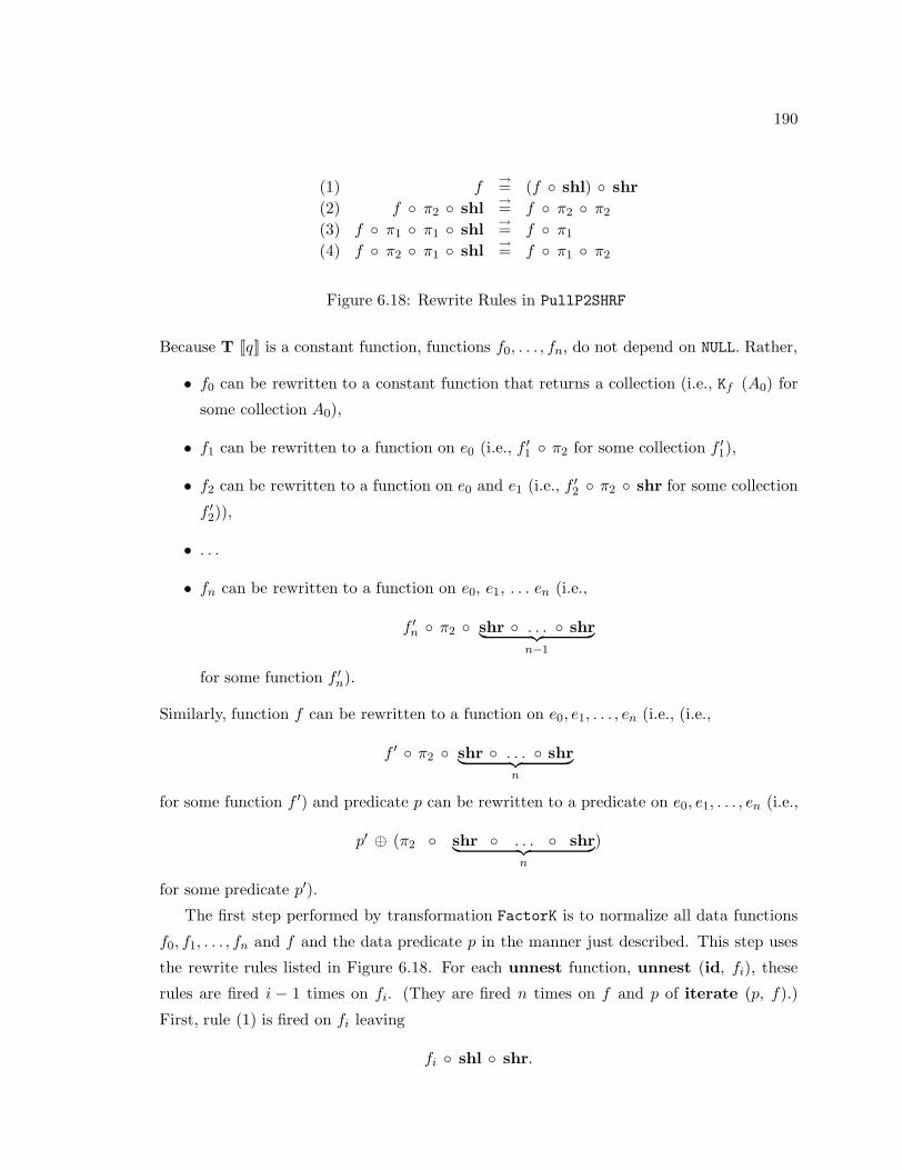
190
(1) f→= (f ◦ shl) ◦ shr
(2) f ◦ π2 ◦ shl →= f ◦ π2 ◦ π2
(3) f ◦ π1 ◦ π1 ◦ shl →= f ◦ π1
(4) f ◦ π2 ◦ π1 ◦ shl →= f ◦ π1 ◦ π2
Figure 6.18: Rewrite Rules in PullP2SHRF
Because T JqK is a constant function, functions f0, . . . , fn, do not depend on NULL. Rather,
• f0 can be rewritten to a constant function that returns a collection (i.e., Kf (A0) for
some collection A0),
• f1 can be rewritten to a function on e0 (i.e., f ′1 ◦ π2 for some collection f ′1),
• f2 can be rewritten to a function on e0 and e1 (i.e., f ′2 ◦ π2 ◦ shr for some collection
f ′2)),
• . . .
• fn can be rewritten to a function on e0, e1, . . . en (i.e.,
f ′n ◦ π2 ◦ shr ◦ . . . ◦ shr︸ ︷︷ ︸n−1
for some function f ′n).
Similarly, function f can be rewritten to a function on e0, e1, . . . , en (i.e., (i.e.,
f ′ ◦ π2 ◦ shr ◦ . . . ◦ shr︸ ︷︷ ︸n
for some function f ′) and predicate p can be rewritten to a predicate on e0, e1, . . . , en (i.e.,
p′ ⊕ (π2 ◦ shr ◦ . . . ◦ shr︸ ︷︷ ︸n
)
for some predicate p′).
The first step performed by transformation FactorK is to normalize all data functions
f0, f1, . . . , fn and f and the data predicate p in the manner just described. This step uses
the rewrite rules listed in Figure 6.18. For each unnest function, unnest (id, fi), these
rules are fired i − 1 times on fi. (They are fired n times on f and p of iterate (p, f).)
First, rule (1) is fired on fi leaving
fi ◦ shl ◦ shr.

191
(iterate (p, f) ◦unnest (id, fn) ◦ unnest (id, fn−1) ◦ . . . ◦ unnest (id, f1) ◦ unnest (id, f0) ◦single) ! NULL
such thatp = p′ ⊕ (π2 ◦ shrn)f = f ′ ◦ π2 ◦ shrn
fi = f ′i ◦ π2 ◦ shri−1 (for i > 0), andf0 = Kf (A)
Figure 6.19: Translated OQL Queries Following Rewriting of their Data Functions
Then, rules (2) and (3) and (4) are successively fired on
fi ◦ shl.
After i− 1 applications of these rules, we are left with a function of the form
f′′i ◦ g ◦ shr ◦ . . . ◦ shr︸ ︷︷ ︸
i−1
.
Note that fi is a function that gets invoked on arguments of the form,
[. . .[NULL, e0], . . . ei−1].
The invocation of
f′′i ◦ g ◦ shr ◦ . . . ◦ shr︸ ︷︷ ︸
i−1
.
on this argument reduces to
f′′i ! (g ! [NULL, [e0, . . .[ei−2, ei−1] . . .]]).
As fi ignores NULL, g must be π2. Therefore, the effect of this step is to leave a query
expression of the form shown in Figure 6.19.
The rest of this transformation proceeds in five steps and uses the rules of Figure 6.20.
In this figure and in the text, we use the notation “δi” to denote a KOLA function defined
for i ≥ 0 as follows:δ0 = shr
δi = 〈π1, δi−1 ◦ π2〉, for i > 0
Substituting for δ in rules (10) and (11) of Figure 6.20 reveals these rules to be strictly
unnecessary: rule (11) follows from rule (7), and rule (12) follows from rule (9) (fired n

192
(1) iterate (p ⊕ (f ◦ h), g ◦ h) ◦ unnest (h1, h2) →=iterate (p ⊕ f, g) ◦ unnest (h ◦ h1, h2)
(2) unnest (f ◦ shr ◦ shr, g ◦ shr) ◦ unnest (h1, h2) →=unnest (f ◦ δ1 ◦ shr, g) ◦ unnest (shr ◦ h1, h2)
(3) unnest (f ◦ π2 ◦ shr, g ◦ π2) ◦ unnest (h1, h2) →=unnest (f, g) ◦ unnest (π2 ◦ h1, h2)
(4) unnest (π2 ◦ shr, f ◦ π2) ◦ unnest (id, Kf (A)) ◦ single →=Kf (unnest (id, f) ! A)
(5) f ◦ Kf (x) →= Kf (f ! x) (6) f→= f ◦ shl ◦ shr
(7) π2 ◦ 〈f, g〉 →= g (8) f ◦ id →= f
(9) shr ◦ 〈π1, f ◦ π2〉 ◦ shl →= 〈π1, 〈π1, f ◦ π2〉 ◦ π2〉
(10) π2 ◦ δi→= δi−1 ◦ π2 (11) shri ◦ δ1 ◦ shli →= δi+1
Figure 6.20: Rewrite Rules in FactorK and FKAux
times). In fact the COKO implementations of these transformations cannot express rules
(10) and (11) (and instead would fire rules (7) and (10) as many times as necessary) because
the matching of these rules to queries would require counting. (Note however that we can
fire rule (2) once we substitute 〈π1, shr ◦ π2〉 for δ1.) We include these “macro rules” here
to simplify the description of this transformation.
The normalization firing algorithm proceeds by visiting each subfunction of the form,
f ◦ g of the query shown in Figure 6.19. Therefore, the first subfunction visited is
iterate (p, f) ◦ unnest (id, fn),
the second is
unnest (id, fn) ◦ unnest (id, fn−1)
(modulo the normalizations of p, f and fn and the changes made to unnest (id, fn) after
visiting the first subfunction) and so on. These visits are described below.
Step 1: Substituting for p and f , the first visited subfunction is
iterate (p′ ⊕ (π2 ◦ shrn), f ′ ◦ π2 ◦ shrn) ◦ unnest (id, fn).

193
Rule (1) of Figure 6.20 fires on this function n + 1 times, and rule (9) fires once, leaving a
query of the form,
(iterate (p′, f ′) ◦unnest (π2 ◦ shrn, fn) ◦ unnest (id, fn−1) ◦ . . . ◦ unnest (id, f1) ◦ unnest (id, f0) ◦single) ! NULL
such that p′, f ′ and fi are as defined in Figure 6.19.
Step 2: In this step, each pair of adjacent unnest subfunctions in the composition chain,
unnest (π2 ◦ shrn, fn) ◦ unnest (id, fn−1) ◦ . . . ◦ unnest (id, f0)
is visited in turn. The purpose of this is to “push” the data function “π2 ◦ shrn” from the
left-most unnest function into the unnest functions to its right. Each “push” loses one of
the “shr” subfunctions, and so the effect of this step is to rewrite the above composition
chain intounnest (gn, fn) ◦unnest (gn−1, fn−1) ◦. . . ◦unnest (g2, f2) ◦unnest (π2 ◦ shr, f1) ◦unnest (id, f0)
for some functions g2, . . . , gn.
Substituting for fi, the visit of the (n− i + 1)th pair of unnest functions,
unnest (π2 ◦ shri, f ′i ◦ π2 ◦ shri−1) ◦ unnest (id, fi−1)
pushes the data function “π2 ◦ shri−1” out of the left unnest function and into the right.
This is captured by the “macro rule”,
unnest (π2 ◦ shri, f ◦ π2 ◦ shri−1) ◦ unnest (id, g ◦ π2 ◦ shri−2) →=
unnest (F , f) ◦ unnest (π2 ◦ shri−1, g ◦ π2 ◦ shri−2)
for some function F . Again, this rule is not expressible in COKO and instead we specify a
COKO transformation that achieves the same result with the KOLA rules of Figure 6.20.
In visiting the (n− i + 1)th pair of unnest functions (for i ≥ 2),
unnest (π2 ◦ shri, f ′i ◦ π2 ◦ shri−1) ◦ unnest (id, fi−1),

194
this transformation first fires rule (2) and rule (8), leaving:
unnest (π2 ◦ shri−2 ◦ δ1 ◦ shr, f ′i ◦ π2 ◦ shri−2) ◦ unnest (shr, fi−1).
Next, rule (6) fires i− 2 times, leaving:
unnest (π2 ◦ γ ◦ shri−1, f ′i ◦ π2 ◦ shri−2) ◦ unnest (shr, fi−1).
such that
γ = shri−2 ◦ δ1 ◦ shli−2.
The firing of “macro rule” (11) (equivalently, (i− 2) firings of rule (9)) on γ leaves:
unnest (π2 ◦ δi−1 ◦ shri−1, f ′i ◦ π2 ◦ shri−2) ◦ unnest (shr, fi−1).
Then, the firing of “macro rule” (10) (equivalently, rule (7)) leaves:
unnest (δi−2 ◦ π2 ◦ shri−1, f ′i ◦ π2 ◦ shri−2) ◦ unnest (shr, fi−1).
This pass is repeated for every occurence of “shr” that needs to be passed from right
to left. In this case, (i− 1) passes are completed in all, leaving
unnest (δi−2 ◦ . . . ◦ δ0 ◦ π2 ◦ shr, f ′i ◦ π2) ◦ unnest (shri−1, fi−1).
Subsequently, rule (3) fires, leaving:
unnest (δi−2 ◦ . . . ◦ δ0, f ′i) ◦ unnest (π2 ◦ shri−1, fi−1)
and, substituting for fi−1 the next adjacent pair of unnest functions,
unnest (π2 ◦ shri−1, f ′i ◦ π2 ◦ shri−2) ◦ unnest (id, fi−2)
is visited. In all, n− 1 visits are made of adjacent unnest functions, leaving a query of the
form,
(iterate (p′, f ′) ◦unnest (δn−2 ◦ . . . ◦ δ0, f ′n) ◦ unnest (δn−3 ◦ . . . ◦ δ0, f ′n−1) ◦. . . ◦unnest (δ0, f ′2)
unnest (π2 ◦ shr, f ′1 ◦ π2) ◦ unnest (id, Kf (A)) ◦ single) ! NULL.

195
Transformation Figure No. Rules No. Verified No. Lines inRules Firing Algorithm
NormTrans 6.15 4 3 14OrdUnnests 6.16 1 0 7FactorK 6.20 13 9 15Total – 18 12 36
Table 6.4: Analysis of the COKO Normalization Transformations
Steps 3, 4 and 5: In the next step,
unnest (π2 ◦ shr, f ′1 ◦ π2) ◦ unnest (id, Kf (A)) ◦ single
is rewritten by rule (4) leaving
(iterate (p′, f ′) ◦unnest (δn−2 ◦ . . . ◦ δ0, f ′n) ◦ unnest (δn−3 ◦ . . . ◦ δ0, f ′n−1) ◦. . . ◦unnest (δ0, f ′2) ◦ Kf (unnest (id, f ′1) ! A)) ! NULL.
Then, rule (5) is fired in bottom-up fashion, leaving
Kf (iterate (p′, f ′) !
(unnest (δn−2 ◦ . . . ◦ δ0, f ′n) ! (unnest (δn−3 ◦ . . . ◦ δ0, f ′n−1) ! . . . !
(unnest (δ0, f ′2) ! (unnest (id, f ′1) ! A)))))) ! NULL.
Thus, the original query expression has been rewritten to the form Kf (A) ! NULL fos eome
collection A.
Analysis
Table 6.4 summarizes the transformations required to perform the normalization of trans-
lated KOLA queries. As before, the normalization is expressed with little code (fewer than
40 lines of firing algorithm code) and mostly in terms of rewrite rules.
Transformation NormTrans has been tested with over 100 Query Lite and OQL queries
of varying complexity, including the Query Lite query of Figure 6.3 and the OQL queries
of Figures 6.6a and 6.17b.8
8As yet this transformation does not work over queries nested in their SELECT clauses such as that ofFigures 6.6b.

196
SELECT sFROM s IN SensWHERE s.reps.lgst cit.popn > 1M
a. Query Lite Query 1
iterate (gt ⊕ 〈id, Kf (10)〉 ⊕ popn ⊕ lgst cit ⊕ reps, id) ! Sens
b. Its Normalization
join ((((p1 & p2) ⊕ π2) & p3) ⊕ shr, π1 ◦ π1) ![join (Kp (true), id) ! [Sens, Sts], Cits]
such thatp1 = gt ⊕ 〈id, Kf (1M)〉 ⊕ popn ⊕ π2
p2 = eq ⊕ 〈lgst cit ◦ π1, OID ◦ π2〉p3 = eq ⊕ 〈reps ◦ π1, OID ◦ π2〉
c. Its Rewrite by PEWhere
SELECT sFROM s IN Sens, r IN Sts, c IN CitsWHERE (c.popn > 1M) AND (r.lgst cit == c.OID) AND (s.reps == r.OID)
d. Its Translation Into SQL
Figure 6.21: Query 1 (a), Normalization (b), Rewrite by PEWhere (c) In SQL (d)

197
SELECT s
FROM s IN SensWHERE (s.reps.lgst cit.popn > 1M) AND
(s.terms > 5) AND(s.reps.lgst cit.mayor.bornin.popn > 1M)
a. Query Lite Query 2
iterate ((gt ⊕ 〈id, Kf (1M)〉 ⊕ popn ⊕ lgst cit ⊕ reps) &(gt ⊕ 〈id, Kf (5)〉 ⊕ terms) &(gt ⊕ 〈id, Kf (1M)〉 ⊕ popn ⊕ bornin ⊕ mayor ⊕ lgst cit ⊕ reps), id) !
Sens
b. Its Normalization
join (((((((((((p1 & p2) ⊕ π2) & p3 & p4) ⊕ π2) & p5) ⊕ π2) &((p6 & p7) ⊕ 〈π1, (π1 ◦ π2)〉)) ⊕〈π1, 〈π1 ◦ π1, shr ◦ 〈π2 ◦ π1, π2〉〉 ◦ π2〉) ⊕ shr) ⊕〈〈π1 ◦ π1 ◦ π1, shr ◦ 〈〈π2 ◦ π1, π2〉 ◦ π1, π2〉〉 ◦ π1, π2〉),
π1 ◦ 〈π1 ◦ π1 ◦ π1, shr ◦ 〈〈π2 ◦ π1, π2〉 ◦ π1, π2〉〉 ◦ π1) ![join (Kp (true), id) ![join (Kp (true), id) ![join (Kp (true), id) ! [Sens, Sts], Cits], Mays], Cits]
such thatp1 = gt ⊕ 〈id, Kf (1M)〉 ⊕ popn ⊕ π2
p2 = eq ⊕ 〈bornin ◦ π1, OID ◦ π2〉p3 = eq ⊕ 〈mayor ◦ π1, OID ◦ π1 ◦ π2〉p4 = gt ⊕ 〈id, Kf (1M)〉 ◦ popn ⊕ π1
p5 = eq ⊕ 〈lgst cit ◦ π1, OID ◦ π1 ◦ π2〉p6 = gt ⊕ 〈id, Kf (5)〉 ⊕ terms ⊕ π1
p7 = eq ⊕ 〈reps ◦ π1, OID ◦ π2〉
c. Its Rewrite by PEWhere
SELECT sFROM s IN Sens, r IN Sts, c IN Cits, m IN Mays, x IN CitsWHERE (x.popn > 1M) AND (m.bornin == x.OID) AND
(c.mayor == m.OID) AND (c.popn > 1M) AND(r.lgst cit == c.OID) AND (s.terms > 5) AND (s.reps == r.OID)
d. Its Translation Into SQL
Figure 6.22: Query 2 (a), Normalization (b), Rewrite by PEWhere (c) In SQL (d)

198
SELECT s
FROM s IN SensWHERE s.bornin.mayor.terms < 4 AND
s.pty.name == ‘‘GOP’’ ANDs.reps.lgst cit.mayor.bornin.popn > 1M ANDNOT (s.bornin.popn > 1M) ANDs.reps.popn > 10M ANDs.reps.lgst cit.mayor.terms < 3 ANDs.terms > 5 ANDs.bornin.mayor.pty == ‘‘Dem’’ ANDNOT (s.reps.lgst cit.name == ‘‘Providence’’)
a. Query Lite Query 3
iterate ((lt ⊕ 〈id, Kf (40)〉 ⊕ terms ⊕ mayor ⊕ bornin) &(eq ⊕ 〈id, Kf (GOP)〉 ⊕ name ⊕ pty) &(gt ⊕ 〈id, Kf (1M)〉 ⊕ popn ⊕ bornin ⊕ mayor ⊕ lgst cit ⊕ reps) &(∼ (gt) ⊕ 〈id, Kf (1M)〉 ⊕ popn ⊕ bornin) &(gt ⊕ 〈id, Kf (10M)〉 ⊕ popn ⊕ reps) &(lt ⊕ 〈id, Kf (30)〉 ⊕ terms ⊕ mayor ⊕ lgst cit ⊕ reps) &(gt ⊕ 〈id, Kf (50)〉 ⊕ terms) &(eq ⊕ 〈id, Kf (‘‘Dem’’)〉 ⊕ pty ⊕ mayor ⊕ bornin) &(∼ (eq) ⊕ 〈id, Kf (‘‘Providence’’)〉 ⊕ name ⊕ lgst cit ⊕ reps), id) !
Sens
b. Its Normalization
Figure 6.23: Query 3 (a), Normalization (b), . . .

199
join ((((((((p1 & p2) ⊕ π2) & (p3 & p4)) ⊕ π2) &(((((((((((p5 & p6 & p7) ⊕ π2) & ((p8 & p9) ⊕ 〈π1, π1 ◦ π2〉)) ⊕ π2) &((p10 & p11) ⊕ 〈π1, π1 ◦ π2〉)) ⊕ π2) &((p12 & p13) ⊕ 〈π1, π1 ◦ π2〉)) & p14) ⊕ π1) & p15) ⊕〈π1, π1 ◦ π2〉)) ⊕ shr) ⊕ 〈〈〈π1 ◦ π1 ◦ π1 ◦ π1, 〈π2 ◦ π1 ◦ π1 ◦ π1, shr◦ 〈〈π2 ◦ π1, π2〉 ◦ π1), π2〉〉〉 ◦ π1, π2〉 ◦ π1, π2〉,
π1 ◦ π1 ◦ 〈〈π1 ◦ π1 ◦ π1 ◦ π1, 〈π2 ◦ π1 ◦π1 ◦ π1, shr ◦ 〈〈π2 ◦ π1, π2〉 ◦ π1, π2〉〉〉 ◦ π1, π2〉 ◦ π1) ![join (Kp (true), id) ![join (Kp (true), id) ![join (Kp (true), id) ![join (Kp (true), id) ![join (Kp (true), id) ! [Sens, Sts], Cits], Mays], Cits], Cits], Mays]
such thatp1 = eq ⊕ 〈OID, Kf (‘‘Dem’’)〉 ⊕ ptyp2 = lt ⊕ 〈OID, Kf (40)〉 ⊕ termsp3 = ∼ (gt) ⊕ 〈OID, Kf (1)〉 ◦ popn ⊕ π1
p4 = eq ⊕ 〈mayor ◦ π1, OID ◦ π2〉p5 = gt ⊕ 〈OID, Kf (1)〉 ◦ popn ⊕ π2
p6 = lt ⊕ 〈OID, Kf (30)〉 ◦ terms ⊕ π1
p7 = eq ⊕ 〈bornin ◦ π1, OID ◦ π2〉p8 = ∼ (eq) ⊕ 〈OID, Kf (‘‘Providence’’)〉 ◦ name ⊕ π1
p9 = eq ⊕ 〈mayor ◦ π1, OID ◦ π2〉p10 = gt ⊕ 〈OID, Kf (1)〉 ◦ popn ⊕ π1
p11 = eq ⊕ 〈lgst cit ◦ π1, OID ◦ π2〉p12 = eq ⊕ 〈OID, Kf (‘‘GOP’’)〉 ◦ pty ⊕ π1
p13 = eq ⊕ 〈reps ◦ π1, OID ◦ π2〉p14 = gt ⊕ 〈OID, Kf (50)〉 ◦ terms ⊕ π1
p15 = eq ⊕ 〈bornin ◦ π1 ◦ π1, OID ◦ π2〉
c. Its Rewrite by PEWhere
SELECT s
FROM s IN Sens, r IN Sts, c IN Cits, m IN Mays, x IN Cits, y IN Cits, z IN MaysWHERE (z.pty == ‘‘Dem’’) AND (z.terms < 4) AND (NOT (y.popn > 1M)) AND
(y.mayor == z.OID) AND (x.popn > 1M) AND (m.terms < 3) AND(m.bornin == x.OID) AND (NOT (c.name == ‘‘Providence’’)) AND(c.mayor == m.OID) AND (r.popn > 1M) AND (r.lgst cit == c.OID) AND(s.pty == ‘‘GOP’’) AND (s.reps == r.OID) AND(s.terms > 5) AND (s.bornin == y.OID)
d. Its Translation Into SQL
Figure 6.24: Query 3 (cont.) . . ., Rewrite by PEWhere (c) In SQL (d)

200
6.3.3 Transforming Path Expressions to Joins
This section describes a COKO transformation (PEWhere) that rewrites Query Lite queries
with path expressions in their WHERE clause into SQL join queries. Specifically, Query
Lite queries that are translated and then normalized with the transformations described in
Section 6.3.2 are those affected by PEWhere and its auxiliary transformation, PEWAux.
Unlike those of the previous section, the COKO transformations described in this section
are few (2 in all) and short, requiring 3 rewrite rules, 2 inference rules and fewer than 20 lines
of firing algorithm code in all. In addition, the transformations presented here demonstrate
a novel application of the semantic query rewrite facility described in Chapter 5. The
semantic property concerns foreign keys.
Path Expression Elimination Overview
Consider Query Lite Query 1 of Figure 6.21a that finds all Senators in Sens who represent
states whose largest cities have a population of over 1 million people. This query includes
the path expression,
s.reps.lgst cit.popn
in its WHERE clause to find the population of the largest city in the state represented by
Senator s. Specifically, for any Senator s:
• s.reps returns the object denoting the state that s represents,
• s.reps.lgst cit returns the object denoting the largest city of the state that s rep-
resents, and
• s.reps.lgst cit.popn returns the integer denoting the population of the largest city
of the state that s represents.
The relational implementation of San Francisco described in Section 6.1 uses relations to
implement each type extent, with the OID columns as keys. For the object schema of
Figure 2.1,
• Sens is a relation representing the extent of objects of type Senator,
• Sts is a relation representing objects of type Region that are states, and
• Cits is a relation representing objects of type City.

201
As a result, for path expression s.reps.lgst cit.popn, method reps is a foreign key for
Sts, and lgst cit is a foreign key for Cits. This information makes it possible to rewrite
the Query Lite query of Figure 6.21 into the SQL join query,
SELECT s
FROM s IN Sens, r IN Sts, c IN Cits
WHERE (c.popn > 1M) AND (r.lgst cit == c.OID) AND (s.reps == r.OID)
The COKO transformations described in this section perform the rewrite above. These
transformations exploit semantic knowledge of foreign keys (metadata information that is
assumed to be available to the optimizer), to decide when methods in a path expression
can be translated into relational joins. More precisely, these transformations rewrite Query
Lite queries of the form,
SELECT x
FROM x IN A
WHERE Comp1 AND . . . AND Compm
such that each Compi is a simple comparison predicate involving a path expression such as,
x.m0. . . . .mn op k
or
NOT (x.m0. . . . .mn op k).
As well, these transformations have the following characteristics:
• comparisons can appear in the opposite order, as in,
k op x.m0. . . . .mn,
• WHERE clauses can also contain disjunctions provided that the disjunctions disappear
when the WHERE clauses is converted into CNF,
• sharing of path expressions is recognized.
To illustrate sharing, consider Query Lite Query 2 of Figure 6.22a, which finds senators who
have served more than 5 terms, and who represent a state whose largest city: (1) has more
than 1 million people, and (2) has a mayor who was born in a city with more than 1 million
people. This query contains two path expressions that contain the common subexpression,
s.reps.lgst cit.

202
The transformations presented here rewrite this query into the SQL query,
SELECT s
FROM s IN Sens, r IN Sts, c IN Cits, m IN Mays, x IN Cits
WHERE (x.popn > 1M) AND (m.bornin == x.OID) AND
(c.mayor == m.OID) AND (c.popn > 1M) AND
(r.lgst cit == c.OID) AND (s.terms > 5) AND (s.reps == r.OID)
rather than to the more naive translation,
SELECT s
FROM s IN Sens, r IN Sts, c IN Cits, m IN Mays, x IN Cits, r2 IN Sts, c2 IN Cits
WHERE (x.popn > 1M) AND (m.bornin == x.OID) AND
(c.mayor == m.OID) AND (c.popn > 1M) AND
(r.lgst cit == c.OID) AND (s.terms > 5) AND (s.reps == r.OID) AND
(r2.lgst cit == c2.OID) AND (c2.mayor == m.OID) AND (s.reps == r2.OID)
which is a 7-way join rather than a 5-way join, redundantly joining collections Sts and
Cits twice (once for each occurence of the common subexpression).
The transformations described here not only recognize common subexpressions in path
expressions, but do so for:
• any number of path expressions in a WHERE clause,
• any degree of sharing amongst path expressions, and
• any number of path expressions sharing a given subexpression (even when path ex-
pressions with shared subexpressions are not adjacent).
An example application of this transformation is shown in Figures 6.23a. Figure 6.23a and
6.23b show the original Query Lite query and the result of its translation and normalization.
Figure 6.24c show the result of rewriting this query by PEWhere. Figure 6.24d shows this
same query after its translation into SQL.
Query 3 includes path expressions with varying degrees of sharing, such as:
• s.bornin.mayor.terms < 4, which shares:
– s.bornin with: NOT (s.bornin.popn > 1M), and
– s.bornin.mayor with: s.bornin.mayor.pty == ‘‘Dem’’, and
• s.reps.lgst cit.mayor.bornin.popn > 1M , which shares:

203
– s.reps with: s.reps.popn > 1M ,
– s.reps.lgst cit with: NOT (s.reps.lgst cit.name == ‘‘Providence’’), and
– s.reps.lgst cit.mayor with: s.reps.lgst cit.mayor.terms < 3.
The result of rewriting shown in Figure 6.24 exploits this sharing and joins as few collections
as possible.
Transformation PEWhere and Its Auxiliary Transformation
Translation of Query Lite queries generates KOLA expressions of the form,
(iterate (p, id) ◦ unnest (id, Kf (A)) ◦ single) ! NULL.
After normalization using the transformations of Section 6.3.2, these queries are of the form,
iterate (q, id) ! A.
If Query Lite queries have WHERE clauses as characterized in the previous section (i.e., con-
junctions of simple comparisons), then the predicate p in the query produced by translation
is of the form,
p0 & . . . & pm
such that each pi is of the form
op ⊕ 〈min ◦ . . . ◦ m0 ◦ gi, Kf (k)〉
or
∼ (op ⊕ 〈min ◦ . . . ◦ m0 ◦ gi, Kf (k)〉),op is a KOLA comparison primitive (such as eq), each mj is a method primitive and k is a
constant. For these same queries, normalization results in predicates p′ of the form,
op ⊕ 〈id, Kf (k)〉 ⊕ min ◦ . . . ◦ m0 ◦ gi
or
∼ (op) ⊕ 〈id, Kf (k)〉 ⊕ min ⊕ . . . ⊕ m0 ⊕ gi
(as illustrated by the normalized translations of Query Lite Queries: 1 (Figure 6.21b), 2
(Figure 6.22b), and 3 (Figure 6.23b)).
PEWhere (Figure 6.25) gets invoked after translation and normalization, and therefore
affects queries of the form,
iterate (p′1 & . . . & p′m, id) ! A

204
TRANSFORMATION PEWhere-- Transforms QL queries with where predicates of the form,-- x.a1()...an() op k, or k op x.a1()...an()-- into join queries using scoping rules for attributesUSESLBJoin,PEWAux,PullComFunc,SimpFunc,SimpPredBEGIN-- Step 1: Find common subfunctions of conjuncts and factor outGIVEN iterate (p, F) ! O DO PullComFunc (p);
-- Step 2: Call PEWAuxPEWAux;
-- Step 3: Recombine iterate’s and joins into left-bushy join treeLBJoinEND
TRANSFORMATION PEWAuxUSESpe2j: scope (B, f, A) ::
iterate (p ⊕ f, id) ! A −→join (eq ⊕ <f ◦ π1, OID ◦ π2〉, π1) ! [A, iterate (p, id) ! B],
splcon: iterate (p & q, id) ! A −→ iterate (p, id) ! (iterate (q, id) ! A),SimpPred
INFERSScope
BEGINsplcon → GIVEN F ! x DO {PEWAux (x); PEWAux};pe2j → GIVEN join (p, F) ! [ O, B] DO PEWAux (B)
END
Figure 6.25: Transformation PEWhere and its Auxiliary Transformation

205
such as those of Figures 6.21, 6.22 and 6.23. PEWhere operates in 3 steps, which are
demonstrated in terms of their effect on the query of Figure 6.22b: the result of translating
and normalizing the Query Lite Query 2 of Figure 6.22a.
Step 1: In the first step of this transformation, PullComFunc (Section 6.3.1) rewrites
conjunction predicates,
p1 & . . . & qn
into the form,
(q1 ⊕ f1) & . . . & (qm ⊕ fm)
such that m ≤ n and no two functions fi and fj (i 6= j) are the same. This step extracts
the common subexpressions from distinct path expressions.
Applied to Query 2:
When applied to the query of Figure 6.22b, this step results in the expression, Q:
iterate (((q1a & q1b) ⊕ lgst cit ⊕ reps) & q2, id) ! Sens
such that
q1a = gt ⊕ 〈id, Kf (1M)〉 ⊕ popn,
q1b = gt ⊕ 〈id, Kf (1M)〉 ⊕ popn ⊕ bornin ⊕ mayor and
q2 = gt ⊕ 〈id, Kf (5)〉 ⊕ terms.
Step 2: The second step of this transformation invokes auxiliary transformation, PEWAux
on the expression resulting from 1. PEWAux has two key rules. The first is rule splcon,
which splits an iterate function instantiated with a conjunction predicate into two. When
applied to queries of the form,
iterate (q1 & . . . & qm, id) ! A
such as those resulting from Step 1 of PEWhere’s firing algorithm, this rule returns
iterate (q1, id) ! (iterate (q2 & . . . & qm, id) ! A.
The effect of the recursive calls to PEWAux that follow the successful firing of splcon is to
invoke PEWAux successively on subqueries:
• iterate (qm, id) ! A,

206
scope (Sts, reps, Sens).scope (Cits, reps, Mays).scope (Cits, bornin, Sens).scope (Cits, bornin, Mays).
scope (Cits, lgst cit, Rgs).scope (Cits, lgst cit, Sts).
scope (Mays, mayor, Cits).
Figure 6.26: Scope Facts Assumed Known for these Examples
• iterate (qm−1, id) ! (iterate (qm, id) ! A),
• iterate (qm−2, id) ! (iterate (qm−1, id) ! (iterate (qm, id) ! A)), etc.
The second rule, pej2, is a conditional rewrite rule that depends on the condition,
scope (B, f, A). This condition holds of collections A and B and function f if f is a
function on elements of A and is also a foreign key of B. Figure 6.26 shows the scope facts
that are assumed to hold (and to be part of the schema accessible by our optimizer) for the
examples in this chapter.
Figure 6.27 shows a property definition for Scope that lists three inference rules for
inferring this property. The first of these rules,
scope (B, f, A) =⇒ scope (B, f, iterate (p, id) ! A)
says that if f is a foreign key for B that is defined on A, then it is also a foreign key for B
that is defined on any selection on A. The second and third rules,
scope (B, f, A) =⇒ scope (B, f, join (p, π1) ! [A, O]).
scope (B, f, A) =⇒ scope (B, f, join (p, π2) ! [ O, A]).
say that if f is a foreign key for B that is defined on A, then it is a foreign key for B that is
defined on (left and right) semi-joins on A.
Provided that scope is inferred to be true for collection B, function f and collection A,
the query,
iterate (p ⊕ f , id) ! A
can be rewritten to a join of A and the subcollection of B satisfying p:
join (eq ⊕ 〈f ◦ π1, OID ◦ π2〉, π1) ! [A, iterate (p, id) ! B].

207
PROPERTY ScopeBEGINscope (B, f, A) =⇒ scope (B, f, iterate (p, id) ! A).scope (B, f, A) =⇒ scope (B, f, join (p, π1) ! [A, O]).scope (B, f, A) =⇒ scope (B, f, join (p, π2) ! [ O, A]).
END
Figure 6.27: Property Scope and Sample Metadata Infomation Regarding Scope
This query screens B for those elements satisfying p, and then joins the result with A to
return those elements of A whose values for f are represented on the subcollection of B. In
terms of Query Lite queries, the left-hand side of the rule denotes queries of the form,
SELECT x
FROM x IN A
WHERE p (f (x)).
In terms of SQL queries, the right-hand side of the rule denotes queries of the form,
SELECT x
FROM x IN A, y IN B
WHERE f (x) == y AND p (y).
Each time pe2j is successfully fired, it returns a query of the form,
join (eq ⊕ 〈f ◦ π1, OID ◦ π2〉, π1) ! [A, iterate (p, id) ! B],
and PEWAux is called recursively on the second argument to the join,
iterate (p, id) ! B.
This recursive call ensures that all methods appearing in a path expression contribute to
the rewrite into a join query.
Applied to Query 2:
1. First, splcon successfully fires and triggers a recursive call of PEWAux on
iterate (q2, id) ! Sens.

208
Rule pe2j does not successfully fire on this expression (because there is no collection
B such that
scope (B, terms, Sens)
holds.) Therefore, a second recursive call to PEWAux is made on
iterate ((q1a & q1b) ⊕ lgst cit ⊕ reps, id) ! (iterate (q2, id) ! Sens).
2. The call of PEWAux on this query fails to fire splcon, but succeeds in firing pe2j. The
first inference rule for Scope in Figure 6.27 together with the fact,
scope (Sts, reps, Sens),
makes it possible to infer,
scope (Sts, reps, iterate (q2, id) ! Sens),
and therefore pej2 successfully fires. This results in the query,
join (eq ⊕ 〈reps ◦ π1, OID ◦ π2〉, π1) !
[iterate (q2, id) ! Sens, iterate ((q1a & q1b) ⊕ lgst cit, id) ! Sts].
3. The successful firing of rule pe2j triggers another recursive call of PEWAux, this time
on
iterate ((q1a & q1b) ⊕ lgst cit, id) ! Sts.
Again, pe2j successfully fires on this subquery because of the fact,
scope (Cits, lgst cit, Sts).
This leaves the subexpression,
join (eq ⊕ 〈lgst cit ◦ π1, OID ◦ π2〉, π1) !
[Sts, iterate (q1a & q1b, id) ! Cits].
4. Next, PEWAux is recursively called on
iterate (q1a & q1b, id) ! Cits,
or equivalently,
iterate ((gt ⊕ 〈id, Kf (1M)〉 ⊕ popn) &
(gt ⊕ 〈id, Kf (1M)〉 ⊕ popn ⊕ bornin ⊕ mayor), id) ! Cits.
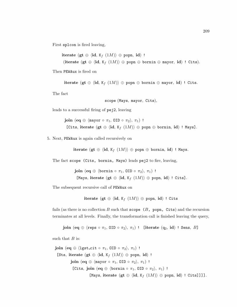
209
First splcon is fired leaving,
iterate (gt ⊕ 〈id, Kf (1M)〉 ⊕ popn, id) !
(iterate (gt ⊕ 〈id, Kf (1M)〉 ⊕ popn ⊕ bornin ⊕ mayor, id) ! Cits).
Then PEWAux is fired on
iterate (gt ⊕ 〈id, Kf (1M)〉 ⊕ popn ⊕ bornin ⊕ mayor, id) ! Cits.
The fact
scope (Mays, mayor, Cits),
leads to a successful firing of pej2, leaving
join (eq ⊕ 〈mayor ◦ π1, OID ◦ π2〉, π1) !
[Cits, iterate (gt ⊕ 〈id, Kf (1M)〉 ⊕ popn ⊕ bornin, id) ! Mays].
5. Next, PEWAux is again called recursively on
iterate (gt ⊕ 〈id, Kf (1M)〉 ⊕ popn ⊕ bornin, id) ! Mays.
The fact scope (Cits, bornin, Mays) leads pej2 to fire, leaving,
join (eq ⊕ 〈bornin ◦ π1, OID ◦ π2〉, π1) !
[Mays, iterate (gt ⊕ 〈id, Kf (1M)〉 ⊕ popn, id) ! Cits].
The subsequent recursive call of PEWAux on
iterate (gt ⊕ 〈id, Kf (1M)〉 ⊕ popn, id) ! Cits
fails (as there is no collection B such that scope (B, popn, Cits) and the recursion
terminates at all levels. Finally, the transformation call is finished leaving the query,
join (eq ⊕ 〈reps ◦ π1, OID ◦ π2〉, π1) ! [iterate (q2, id) ! Sens, B]
such that B is:
join (eq ⊕ 〈lgst cit ◦ π1, OID ◦ π2〉, π1) !
[Sts, iterate (gt ⊕ 〈id, Kf (1M)〉 ⊕ popn, id) !
join (eq ⊕ 〈mayor ◦ π1, OID ◦ π2〉, π1) !
[Cits, join (eq ⊕ 〈bornin ◦ π1, OID ◦ π2〉, π1) !
[Mays, iterate (gt ⊕ 〈id, Kf (1M)〉 ⊕ popn, id) ! Cits]]]].

210
Transformation Figure No. Rules No. Verified No. Lines inRules Firing Algorithm
PEWhere 6.25 1 1 15PEWAux 6.25 2 1 4Scope 6.27 2 2Total – 5 4 19
Table 6.5: Analysis of the Query Lite → SQL Transformations
Step 3: The final step of this transformation converts the query resulting from step 2 into
a left-bushy join. This step is strictly not required, but simplifies the task of converting the
resulting query into SQL as we show in Section 6.4. Applied to the query above, this step
returns the query of Figure 6.22c. Expressed in SQL, this query is:
SELECT s
FROM s IN Sens, r IN Sts, c IN Cits, m IN Mays, x IN Cits
WHERE (x.popn > 1M) AND (m.bornin == x.OID) AND
(c.mayor == m.OID) AND (c.popn > 1M) AND
(r.lgst cit == c.OID) AND (s.terms > 5) AND (s.reps == r.OID)
Analysis
Table 6.5 summarizes the transformations and property presented in this section. Note that
this complex rewrite is expressed with 3 rewrite rules, 2 inference rules and fewer than 20
lines of firing algorithm code.
6.4 Translating KOLA into SQL
Transformation PEWhere leaves Query Lite queries in the form
join (p1 & . . . & pn, f) !
[join (Kp (true), id) !
[join (Kp (true), id) !
[ . . .[join (Kp (true), id) ! [A1, A2], . . .], Am−2], Am−1], Am]
or in the form iterate (p, f) ! A. The sublanguage of KOLA that consists of such expres-
sions only includes primitives: id, π1, π2, shr, shl, OID, m (m a method), abs, add, sub,
mul, div, mod, eq, neq, lt, gt, leq, geq; and formers: 〈 〉, ◦, Kf , Cf , iterate, join , ⊕, &,

211
Basic Function PrimitivesT−1 Jid ! xK = T−1 JxK
T−1 Jπ1 ! [x, y]K = T−1 JxKT−1 Jπ2 ! [x, y]K = T−1 JyK
T−1 Jm ! xK = T−1 JxK .m (for m a unary method)T−1 Jm ! [x, [ . . .[y1, y2], . . . , yn]]K = T−1 JxK .m (T−1 Jy1K, . . . , T−1 JynK)
(for m an n-ary method)
Int and Float Function Primitives (i, j integers or floats)T−1 Jabs ! iK = abs (T−1 JiK)
T−1 Jadd ! [i, j]K = (T−1 JiK) + (T−1 JjK)T−1 Jsub ! [i, j]K = (T−1 JiK) - (T−1 JjK)T−1 Jmul ! [i, j]K = (T−1 JiK) * (T−1 JjK)T−1 Jdiv ! [i, j]K = (T−1 JiK) / (T−1 JjK)
T−1 Jmod ! [i, j]K = (T−1 JiK) MOD (T−1 JjK)Basic Predicate Primitives (x and y of type T )
T−1 Jeq ? [x, y]K = (T−1 JxK) == (T−1 JyK)T−1 Jneq ? [x, y]K = (T−1 JxK) != (T−1 JyK)
T−1 Jisnull ? xK = (T−1 JxK) IS NULLT−1 Jisnotnull ? xK = (T−1 JxK) IS NOT NULL
String and Int Predicate Primitives (x and y strings or integers)T−1 Jlt ? [x, y]K = (T−1 JxK) < (T−1 JyK)T−1 Jgt ? [x, y]K = (T−1 JxK) > (T−1 JyK)
T−1 Jleq ? [x, y]K = (T−1 JxK) <= (T−1 JyK)T−1 Jgeq ? [x, y]K = (T−1 JxK) >= (T−1 JyK)Table 6.6: T−1: Applied to KOLA Primitives

212
∼, Kp, and Cp. Further, all queries in this sublanguage are assumed to be iterate queries,
binary join queries, or left-bushy n-ary join queries.
A translation function, T−1 to translate KOLA expressions over this subset of KOLA
into SQL is defined in Tables 6.6 and 6.7. Note that Table 6.7 includes two translation
definitions for join. The first of these is for translating n-ary joins (n > 2) only. The
second of these is for translating binary joins only.
The following example illustrates this translation function. As shown in Section 6.3.3,
when invoked on Query Lite query 1 of Figure 6.21b, transformation PEWhere returns the
query of Figure 6.21c. This query gets translated into SQL as follows:
T−1
tjoin ((((p1 & p2) ⊕ π2) & p3) ⊕ shr, π1 ◦ π1) !
[join (Kp (true), id) ! [Sens, Sts], Cits]
|
such that
p1 = gt ⊕ 〈id, Kf (1M)〉 ⊕ popn ⊕ π2
p2 = eq ⊕ 〈lgst cit ◦ π1, OID ◦ π2〉p3 = eq ⊕ 〈reps ◦ π1, OID ◦ π1 ◦ π2〉
=
SELECT ((π1 ◦ π1) ! [[s, r], c])
FROM s IN Sens, r IN Sts, c IN Cits
WHERE (((((p1 & p2) ⊕ π2) & p3) ⊕ shr) ? [[s, r], c]).

213
Reducing the predicates in this expression leaves,
SELECT s
FROM s IN Sens, r IN Sts, c IN Cits
WHERE (((((p1 & p2) ⊕ π2) & p3) ⊕ shr) ? [[s, r], c])
=
SELECT s
FROM s IN Sens, r IN Sts, c IN Cits
WHERE ((((p1 & p2) ⊕ π2) & p3) ? [s, [r, c]])
=
SELECT s
FROM s IN Sens, r IN Sts, c IN Cits
WHERE (((p1 & p2) ⊕ π2) ? [s, [r, c]]) AND (p3 ? [s, [r, c]])
=
SELECT s
FROM s IN Sens, r IN Sts, c IN Cits
WHERE ((p1 & p2) ? [r, c]) AND (p3 ? [s, [r, c]])
=
SELECT s
FROM s IN Sens, r IN Sts, c IN Cits
WHERE (p1 ? [r, c]) AND (p2 ? [r, c]) AND (p3 ? [s, [r, c]])
Reducing each subpredicate in turn, we get:
p1 ? [r, c] = (gt ⊕ 〈id, Kf (1M)〉 ⊕ popn ⊕ π2) ? [r, c]
= (gt ⊕ 〈id, Kf (1M)〉 ⊕ popn) ? c
= (gt ⊕ 〈id, Kf (1M)〉) ? (c.popn)
= gt ? [c.popn, 1M]
= c.popn > 1M,
p2 ? [r, c] = (eq ⊕ 〈lgst cit ◦ π1, OID ◦ π2〉) ? [r, c]
= eq ? [(lgst cit ◦ π1) ! [r, c], (OID ◦ π2) ! [r, c]]
= eq ? [r.lgst cit, c.OID]
= r.lgst cit == c.OID, and

214
p3 ? [s, [r, c]] = (eq ⊕ 〈reps ◦ π1, OID ◦ π1 ◦ π2〉) ? [s, [r, c]]
= eq ? [(reps ◦ π1) ! [s, [r, c]], (OID ◦ π1 ◦ π2) ! [s, [r, c]]]
= eq ? [s.reps, r.OID]
= s.reps == r.OID.
Reduction leaves the SQL query,
SELECT s
FROM s IN Sens, r IN Sts, c IN Cits
WHERE (c.popn > 1M) AND (r.lgst cit == c.OID) AND (s.reps == r.OID)
Other examples of translation are shown for the results of rewriting (with transformation
PEWhere) Query Lite queries 1 (Figure 6.21d is the SQL translation of Figure 6.21c), 2
(Figure 6.22d is the SQL translation of Figure 6.22c), and 3 (Figure 6.24d is the SQL
translation of Figure 6.24c).
6.5 Discussion
In this section, we reflect upon our experiences using COKO and KOLA to determine how
well this framework met our integration and ease-of-use goals described at the chapter’s
onset.
6.5.1 Integration Capabilities of COKO-KOLA
COKO-KOLA is a generator of query rewriting components designed to accept queries as
inputs and generate inputs for cost-based optimizers. But how easy is it to integrate these
query rewriters within real query processing environments?
The integration of the COKO-KOLA framework within the San Francisco project re-
quired the development of two translators. The first (described in Section 6.2) translates
Query Lite queries (and more generally, all set and bag-based OQL queries) into KOLA.
The second (described in Section 6.4) translates a subset of KOLA queries into SQL. Of
these translators, the first was by far the easiest to design and implement. This translator
has a similar flavor to the many combinator translations of the lambda calculus (e.g., [27]).
The availability of sophisticated compiler generator tools such as Ox [8] made this part of
the project straightforward.
On the other hand, translation from KOLA to SQL was more tricky. The problem
here was specifying exactly the sublanguage of KOLA that could be translated into SQL.

215
Basic Function FormersT−1 J(f ◦ g) ! xK = T−1 Jf ! (g ! x)KT−1 J〈f, g〉 ! xK = [T−1 Jf ! xK, T−1 Jg ! xK]T−1 JKf (x) ! yK = T−1 JxK
T−1 JCf (f, x) ! yK = T−1 Jf ! [x, y]KBasic Predicate Formers
T−1 J(p ⊕ f) ? xK = T−1 Jp ? (f ! x)KT−1 J(p & q) ? xK = (T−1 Jp ? xK) AND (T−1 Jq ? xK)T−1 J∼ (p) ? xK = NOT (T−1 Jp ? xK)T−1 JKp (b) ? xK = T−1 JbK
T−1 JCp (p, x) ? yK = T−1 Jp ? [x, y]KQuery Function Formers
T−1 Jiterate (p, f) ! AK =SELECT (T−1 Jf ! xK)FROM x IN AWHERE (T−1 Jp ? xK)
T−1
uwwwwvjoin (p, f) ![join (Kp (true), id) ![ . . .[join (Kp (true), id) ![A1, A2], . . . ], An]
}����~=
SELECT (T−1 Jf ! [ . . .[x1, x2], . . .], xn]K)FROM x1 IN A1, . . . , xn IN An
WHERE (T−1 Jp ? [ . . .[x1, x2], . . .], xn]K)T−1 Jjoin (p, f) ! [A1, A2]K =
SELECT (T−1 Jf ! [x1, x2]K)FROM x1 IN A1, x2 IN A2
WHERE (T−1 Jp ? [x1, x2]K)Table 6.7: T−1: Applied to KOLA Formers

216
Some restrictions are easy. For example, flat can never be translated into SQL because the
input to this function (a nested collection) is forbidden by the flatness restrictions of the
relational model. Other restrictions are harder to specify. For example, queries of the form,
iterate (p, f) ! A, can be translated into KOLA, but only in certain cases. For example,
• f cannot be another iterate or join query,
• f can be a composition of some functions (e.g., add ◦ 〈terms, Kf (1)〉) but not others
(e.g., lgst cit ◦ reps) that translate into path expressions.
Our approach to this issue is unsatisfying in the long term. In defining our KOLA → SQL
translation function, T−1, we assumed that inputs were generated from the pipeline of (1)
the Query Lite → KOLA translator, (2) the NormTrans query rewrite, and (3) the PEWhere
rewrite. In fact, T−1 is not defined for all of KOLA, and worse, would translate some
queries that were not produced by the pipeline into queries not recognized by SQL.
The long term solution of this problem will be to somehow characterize useful sublan-
guages of KOLA (depending on the underlying object → relational data model mapping)
that can be translated into SQL. We consider this challenge to be extremely important.
Query rewriting is likely to become the primary technique for reusing query processing soft-
ware with new kinds of queries. San Francisco provides one example of this, extending the
capabilities of the DB2 query processor to handle object-oriented queries. But we foresee
other applications to object database products that want to provide query support for OQL
or SQL3 while using existing optimizer technology, and heterogeneous databases that might
want to rewrite queries expressed over an entire federation of databases into separate queries
specific to the individual databases included within the federation. We believe KOLA to be
an ideal intermediate representation for these efforts, both because of its expressive power
and because KOLA rewrites are verifiable with a theorem prover. But this will require
far more precision in specifying sublanguages of KOLA that will serve as targets for query
rewriting (e.g., the sublanguage of KOLA that can be translated into SQL).
In short, the integration of the COKO-KOLA framework within existing query process-
ing systems requires translation to and from KOLA. Translation to KOLA is not a problem;
already KOLA is expressive enough to express queries in the most complex of query lan-
guages such as OQL, and can be readily extended when it falls short in this regard (e.g.,
as it does presently with respect to lists and arrays). However, translation from KOLA will
often be to a language with less expressive power than KOLA (such as SQL). Understanding
exactly what are interesting sublanguages of KOLA that can be translated (and therefore
is the target for query rewriting) represents a challenging component of future work.

217
6.5.2 Ease-Of-Use of COKO-KOLA
For the San Francisco project, we used COKO-KOLA to generate:
1. a library of general-purpose normalization and simplification transformations (pre-
sented in Section 6.3.1),
2. a normalization to make the KOLA queries resulting from translation from OQL or
Query Lite more intuitive (presented in Section 6.3.2), and
3. a transformation to rewrite Query Lite queries with path expressions in their WHERE
clauses to SQL join queries (presented in Section 6.3.3).
Of these generated rewrites, the third by far was the easiest to write. This transformation
rewrites queries with any number of path expressions, of any length, and with any degree
of sharing. Yet, the transformation itself required fewer than 20 lines of firing algorithm
code. The ease with which this transformation was written is encouraging, as it is exactly
these kinds of transformations that are most likely to be developed for optimizers.
On the other hand, by far the most difficult transformation to write was the translation
normalization transformation, NormTrans, and all of its auxiliary transformations. This
transformation required over 50 rewrite rules, roughly 100 lines of firing algorithm code.
Further, this work is not yet complete. This transformation presently does not normalize
queries that are nested in their SELECT clauses (i.e., iterate or join queries with iterate or
join queries as their data functions). While we believe that this part of the normalization
will not be difficult to add (it will likely require merging the functionality of transformations
SimpFunc and FactorK), the task has clearly proved to be non-trivial.
Of course, it should be remembered that this normalization need only be written once
and users of the COKO-KOLA framework would most likely get NormTrans from a library
of rewrites at their disposal, rather than programming it themselves. But on the other
hand, our experience writing this transformation was revealing in certain deficiencies of
COKO as a programming language and development environment. It is these revelations
that will motivate improvements in future versions of the language and compiler. Amongst
our observations are the following:
COKO’s Control Language This exercise provided quite a bit of experience with
COKO’s language for firing algorithms, and revealed certain parts of the language that
could be improved. One aspect of the language that requires some additional thought is the
association of success values with statements in the language. For some statements (e.g.,

218
rule firings and complex statements), success values are quite natural. COKO provides for
concise expression of algorithms such as that which exhaustively applies a set of rules:
BU {ru1 || . . . || run} → recursive call,
or which conditionally executes a statement (S2) if another statement (S1) succeeds and a
different statement (S3) if it fails:
S1 → S2 || S3.
But for other statements, the success values associated with the statements sometimes ran
counter to the desired flow of control. The most obvious example of this concerns the GIVEN
statement. GIVEN statements have the form,
GIVEN eqn1, . . . , eqnn DO S.
and return a success value of true if all equations, eqni succeed in unifying and false other-
wise. While this success result is desirable sometimes, at other times the desired result is
to return true if all equations succeed in unifying and statement S succeeds. To address
this problem, we could change the default success value for GIVEN statements to return
true if both equations and follow-up statement succeed. Then, one could simulate the old
behavior of GIVEN (i.e., return true if all equations succeed regardless of the success value
of the follow-up statement) by writing:
GIVEN eqn1, . . . , eqnn DO {TRUE S}.
The other part of the firing algorithm language that deserves reconsideration are the
success values associated with “;”-separated statements. Presently, a complex statement,
S1; . . . ; Sn
succeeds if any statement, Si succeeds. Often though, what one desires is for this statement
to succeed if one of a particular subset of statements succeeds. The only way to express
this presently is to preface those statements that should not figure into the determination
of the success value with FALSE, as in:
FALSE {S1}; . . . ; FALSE {Sn}
such that all statements Si would be replaced by FALSE {Si} except for those whose success
should influence the success of the entire complex statement. Ideally however, we would

219
like to avoid the use of TRUE and FALSE statements, as their sole purpose is to circumvent
the default success values of statements. Eliminating these statements may require us to
rethink the entire notion of success values completely, perhaps restricting success values
to rule and transformation invocations and adding if-then-else statements to the firing
algorithm language to express desired control.
Parameterized (or Template) COKO Transformations In Section 6.3.1, we de-
scribed a COKO transformation (LBComp) that has an identical firing algorithm and rewrite
rules to transformation LBConj of Figure 4.10, but for the substitution of one former sym-
bol (◦) for another (&) and one set of variables (function variables) for another (predicate
variables). This example suggests another way that COKO could be improved, by allowing
the definition of parameterized transformations (e.g., LB) such that different instantiations
would generate different COKO transformations (e.g., LB (&, p, q, r) could generate LBConj
while LB (◦, f, g, h) could generate LBComp.
Pattern Matching Associative Formers One of the most time-consuming program-
ming tasks is to account for the various ways that associative functions and predicates (e.g.,
(f ◦ g ◦ h) or (p & q & r)) can be associated. Presently, we address this problem by nor-
malizing functions and predicates in advance so that a certain association can be assumed
(e.g., LBComp and LBConj make compositions and conjunctions left-associative (or “left-
bushy”)). But determining the associative structure guaranteed of transformation results
(when such guarantees are possible) is difficult, and frequently we find ourselves normalizing
perhaps unnecessarily, to ensure that functions and predicates are structured in a particular
way.
In the long term, we believe that a better approach to this problem will be to adapt
our matching algorithm to account for associative function and predicate formers. That is,
under this scheme the pattern,
f ◦ g ◦ h
would match either possible association of compositions,
f ◦ (g ◦ h) or (f ◦ g) ◦ h.
This approach is taken by theorem provers such as LP [46].
Speed of Generated Code The query rewrites that are generated from COKO trans-
formations sometimes have poor performance. For example, while transformation PEWhere

220
performs well on “small queries” such as those of Figures 6.21a and Figures 6.22a, it is
noticeably slower with larger queries such as that of Figure 6.23a, requiring upwards of 3
minutes to perform the desired rewrite on a 200Mz Sparcstation 10.
We need to examine our compiler implementation to find the performance bottleneck,
but there are many areas that could be contributing factors. Among them:
• As described in Chapter 4, our COKO compiler was designed for simplicity rather
than performance. The code it produces generates a parse tree for the compiled
transformations, and then invokes a method (exec) on its root (triggering subsequent
calls to exec in descendants of the tree). This approach was simple and made it easy to
extend the language with new statements (as we did by adding TRUE, FALSE and SKIP
statements, and as is done with the definition of every new COKO transformation).
However, the resulting code frequently has inadequate performance. For example, the
COKO statement,
S1; . . . ; Sn
gets compiled into code that builds a binary parse tree of minimum height n, as each
“;” appears as a node in the tree with the two statements it separates as its immediate
children. This design results in a great deal of information passing (e.g., environments
of pattern variables must be passed between parse tree nodes) and thereby puts a
strain on performance. Further, the generated parse trees can be so large that the
C++ compiler cannot generate the code that builds them. We have often been forced
to “break up” COKO transformations into separate subparts in order to get around
this deficiency.
• In Chapter 4, we showed an example of the kinds of efficiency one can get by having
fine control of rule firing. Transformation CNF exhibited far better performance with
a sophisticated and selective firing algorithm, then it did when implemented as an
algorithm that exhaustively applies deMorgan rules.
Unfortunately, we have not yet developed a methodology for developing efficient fir-
ing algorithms such as that for CNF. Many of the algorithms used for the rewrites
presented in this chapter are naive in their application of rewrite rules. For exam-
ple, transformation PCFAux, an auxiliary transformation to PullComFunc that col-
lapses subpredicates with common subfunctions (see Section 6.3.1), uses an algorithm
analagous to a bubble-sort algorithm in order to compare subfunctions appearing in
a predicate. Part of the problem lies with the inherent limitations of the rule-based
221
approach which demands that algorithms be composed from local operations (indi-
vidual rule firings). But at the very least, the performance of firing algorithms used in
our library of common normalizations and simplifications should be improved, given
how often these transformations are likely to be used. But we look forward to future
study of a methodology for writing firing algorithms that minimizes failed rule firings,
achieving for all transformations what we were able to achieve for CNF.
• As described in Chapter 5, our implementation of semantic query rewrites invokes a
Prolog interpreter druing rewriting to issue a semantic query. As in the case of PEWAux,
semantic queries can be posed numerous times during the course of rewriting. (For ex-
ample, in rewriting the relatively simple query of Figure 6.22a, the conditional rewrite
rule, pe2j was fired 9 times (succeeding 4 times).) Each call to the Prolog interpreter
incurs a tremendous amount of overhead from loading and initializing the interpreter,
and converting to and from Prolog representations of KOLA expressions. We believe
that performance of generated rewrites will improve greatly once our Prolog-based im-
plementation of semantic query rewrites is replaced by specialized pattern matching
routines for KOLA trees.
In short, the message from our experience is that the COKO-KOLA framework poten-
tially has much to offer in the development of “real-world” query rewriters given its formal
foundation. But for this potential to be realized, its implementation must grow beyond its
present prototype status. We were especially encouraged by the concise and elegant manner
with which we were able to express the path expression-to-join query rewrite described in
Section 6.3.3. This rewrite exploited all facets of the COKO-KOLA framework, includ-
ing the semantic rewrite facility in order to infer knowledge of foreign keys, and recursive
firing algorithms to ensure the handling of an unbounded number of path expressions of
unbounded length and unbounded degree of subexpression sharing. But while our imple-
mentation is adequate as a proof of concept, it still is only a research prototype.
6.6 Chapter Summary
In this chapter, we have described our experiences using the COKO-KOLA framework
presented in the preceding three chapters. Our challenge was to use COKO-KOLA to
develop a query rewriting facility for an experimental language for the IBM San Francisco
project. The query rewriter developed would translate object-oriented queries expressed in
a simple object-oriented query language, into equivalent SQL queries over the underlying

222
relational implementation of the object-oriented database.
This project alllowed us to determine the ease with which generated rewrites could
be integrated within existing query processor environments, and with which “real” query
rewrites could be expressed. To support integration, we built translators to translate Query
Lite and OQL queries into KOLA, and to translate KOLA queries into SQL. This work
revealed a challenging future direction in specifying sublanguages of KOLA equivalent in
expressive power to other known languages (e.g., SQL), but also showed our framework
to be easily integrated into existing query processor settings. To assess ease of use, we
analyzed the size and effort required to build COKO transformations that were general
purpose normalization and simplification routines, normalizations specific to the result of
translation, and Query Lite → SQL rewrites. Surprisingly, the library of normalizations
(especially the normalization of translated queries) proved most difficult to build. But the
experience revealed to us deficiencies in the COKO language and compiler implementation
that must be addressed in future versions. Most encouraging to us was the ease with which
we were able to write the transformation that did the “actual work” of the query rewrite.
Transformations PEWhere and PEWAux required few rules and few lines of firing algorithm
code to express a powerful and useful query rewrite.

Chapter 7
Dynamic Query Rewriting
In Chapters 3, 4 and 5, we proposed a framework for the expression of query rewrites. In
Chapter 3, we presented KOLA: a combinator-based query algebra and representation that
supports the expression of simple query rewrites with declarative rules. In Chapter 4, we
introduced COKO: a language for expressing complex rewrites in terms of sets of KOLA
rules and firing algorithms. And in Chapter 5, we introduced extensions to COKO and
KOLA that made it possible to express rewrites whose correctness depended on semantic
properties of queries and data. All of the rewrites presented in these chapters are verifiable
with a theorem prover. This is due to the combinator flavor of KOLA that makes it possible
to express subexpression identification and query formulation without code.
In this chapter, we consider another benefit arising from KOLA. This work concerns
when query rewrites get fired rather than how they get expressed. An intelligent decision
about how to rewrite or evaluate a query requires knowing the representations and contents
of the collections involved (e.g., whether or not collections are indexed, sorted, or contain
duplicates). Dynamic query rewriting (query rewriting that takes place during the query’s
evaluation) incorporates this philosophy in settings where this information is not known
until data is accessed (i.e., until run-time). Such settings include:
• object databases that permit queries on anonymous, embedded collections whose con-
tents and representations might only become apparent at run-time,
• network databases (e.g., web databases) that permit queries on collections whose avail-
ability can vary every time the query is executed, and
• heterogeneous databases that permit queries on collections maintained by local databases
with data models and storage techniques known only to them.
223

224
Dynamic query rewriting requires that a query evaluator identify subexpressions of the
processed query, and formulate new queries to ship to the query rewriter for further pro-
cessing. Because KOLA simplifies the expression of these tasks, it is an ideal underlying
query representation.
The work described in this chapter is ongoing and focuses on the application of dynamic
query rewriting to object databases. We have designed a dynamic query rewriter for the
ObjectStore object-oriented database [67], and an implementation of this design is in devel-
opment.1 We present this design using the “NSF” query (NSF2 of Figure 2.6) as a running
example. After presenting the design of the dynamic query rewriter for ObjectStore in
Section 7.1, we trace the evaluation and rewriting of this query in Section 7.2. Finally, we
consider some performance issues that have yet to be addressed and again look at the role
of KOLA in the design of the query rewriter in Section 7.3, before summarizing the chapter
in Section 7.4.
7.1 A Dynamic Query Rewriter for ObjectStore
The potential heterogeneity of collections in an object database makes it sometimes appro-
priate for evaluation strategies to vary from object to object. In Chapter 2, we introduced
the query NSF2 (Figure 2.6) that pairs every bill concerning the NSF with the largest cities
in the regions represented by the bill’s sponsors. The collection of bills queried (Bills)
can contain both House and Senate resolutions whose sponsors are sets of House Repre-
sentatives and Senators respectively. The path expression, x.reps.lgst cit, that finds the
largest city in the region represented by legislator x, is an injective function over objects
of type Representative, but not over objects of type Senator. Therefore, a semantic query
rewrite to eliminate redundant duplicate elimination (as described in Section 5.1) must be
applied selectively to affect the processing of House resolutions but not the processing of
Senate resolutions. Dynamic query rewriting is query rewriting that occurs during a query’s
evaluation (i.e., at run-time). Selective processing of NSF2 can be achieved by firing the du-
plicate elimination query rewrite dynamically as bills are retrieved and their origins (House
or Senate) identified.
We have designed a dynamic query rewriter and query evaluator for ObjectStore [67],
and the implementation and evaluation of this design is ongoing work. This design deviates
from the traditional query processor architecture presented in Chapter 1 (Figure 1.1). The1ObjectStore already performs a limited form of dynamic query optimization involving run-time exploita-tion of indexes, but does nothing by way of dynamic query rewriting.

225
Metadata
Query
Query Representation
Query Representation
Partial Query Plan
Data
Translator
Query Rewriter
Plan Generator
Semantic Condition Checker
Query Evaluator
B
A
QueryRepresentation
Evaluation
Optimization
Conditions
Figure 7.1: An Alternative Architecture for Object Database Query Processors
new architecture (illustrated in Figure 7.1) introduces a feedback loop between evaluation
and rewriting (labeled A in Figure 7.1), as well as incorporating the semantic rewrite com-
ponents described in Chapter 5 (B). The input to the evaluator is not a complete plan, but a
partial plan with “holes” left for those parts of the plan that will be generated dynamically.
To implement this architecture, our design includes two components:
• a plan language that permits expression of partial plans, and
• a query evaluator with hooks back to the optimizer.
After describing these two components, we demonstrate their intended behavior with respect
to the processing of query NSF2.
7.1.1 Making ObjectStore Objects Queryable
The present design of our dynamic query rewriter processes queries over ObjectStore. Our
eventual goal is for this design to be usable with other databases also. Therefore, a design

226
OSObject
kola (): KObject
OSBool
kola (): KBool
OSIterator
open (): Bool
close (): Boolnext (): OSObject
finished (): Boolset (): OSIterator
OSSieve
. . .
OSStr
val: String
OSInt
val: Int
. . .
i2: OSIterator
OSNestedLoopSieve
f: KFunctiong: KFunction
i1: OSIterator
OSRegion
name (): OSStrcapt (): OSCity
OSLegislator
name (): OSStrreps (): OSRegionpty (): OSStr
terms (): OSInt
bornin (): OSCitycities (): OSSourcelu (): OSStrpopn (): OSInt
. . .
OSSource
c: OSCollection
i2: OSIterator
OSMergeSieve
f: KFunctiong: KFunction
i1: OSIterator
OSFilterSieve
p: KPredicate
i: OSIterator
OSMapSieve
f: KFunctioni: OSIterator
OSBasicSieve
p: KPredicate
f: KFunctioni: OSIterator
Figure 7.2: The ObjectStore Queryable Class Hierarchy
goal was to maintain a loose coupling between the rewriter and ObjectStore.
Loose coupling is achieved by maintaining separate class hierarchies for ObjectStore
objects (which can be stored in an ObjectStore database) and KOLA objects (which can
be appear in queries). Because of this design, ObjectStore’s implementation requires no
modification to account for KOLA querying, and our design need not be restricted to
processing ObjectStore objects. The cost of this decision is redundancy in the two class
hierarchies, and the need to translate between the two representations during a query’s
evaluation. Because of the latter issue, a non-prototype design of the dynamic query rewriter
would likely integrate the two object representations.
The only requirement we introduce of queryable ObjectStore objects is that they belong
to a subclass of a class we provide (OSObject). All attributes of these classes should
also have types that are subclasses of OSObject (or OSBool if they are boolean-valued
attributes). This ensures that all classes of objects maintained in the database will have
a KOLA translation function inherited from OSObject and OSBool (kola), even though
designers of such classes may not be aware of this. Other queryable ObjectStore object

227
classes are provided as part of our design (e.g., basic classes such as strings (OSStr) and
integers (OSInt)) as is illustrated in the ObjectStore class hierarchy presented in Figure 7.2.
Figure 7.2 includes two of the classes defined for the Thomas database of Section 2 —
OSLegislator (Legislator) and OSRegion (Region). Subtypes could be be defined to inherit
from these classes (e.g., State could be defined as a subtype of Region in this way). This
figure also includes a subhierarchy of iterators rooted at OSIterator. While instances of
these classes are data (returned as the results of collection generating queries), the classes
themselves comprise the plan language for KOLA. This design is described below.
7.1.2 Iterators
The result of a query can be very large. If a query returns a collection, this collection might
contain many objects (i.e., the result might have a large cardinality). As well, each object in
the result might include other collections and other complex objects as attributes (i.e., the
result might have a large arity also). Thus, it would be inappropriate for a query processor
to return a query result “all at once” and instead a more lazy approach is called for.
Like many query processors (e.g., Exodus [13]) KOLA’s plan language merges query
results with the plans to retrieve them. An iterator is a view for a given collection with a
specialized interface that provides access to the collection one element at a time. Queries
that construct collections in fact return iterators. Thus, iterators serve as both data and
plan.
Our design defines several kinds of iterators (all subclasses of OSIterator) that can be
returned as the result of a query. There is at least one iterator per KOLA query former or
primitive, although not all are shown in Figure 7.2. Designed in an object-oriented style,
each iterator is obligated to provide implementations of the following methods:
• open: which opens all files required by the iterator to retrieve elements, and which
initializes any data structures required for processing,
• next: which returns the next element of the collection maintained by the iterator,
• finished: which returns true if there are no more elements to return,
• close: which closes all files and data structures opened or created by the iterator,
and
• set: which constructs a new stored collection (and accompanying iterator) with du-
plicates removed.2
2Set builds a new stored collection, because our assumption is that duplicate elimination is necessary

228
Thus, if one views a plan language as a collection of algorithms, the method implementations
for the collection of iterators comprise the KOLA plan language.
Iterators can range over collections stored on disk (access methods), or collections gen-
erated on the fly (query operators). Our design introduces the class OSSource to act as
the supertype of all access method iterators, and OSSieve to act as the supertype of all
query operator iterators. Examples of the latter include OSBasicSieve, OSMapSieve and
OSFilterSieve. Objects of class OSBasicSieve act as a view with respect to some KOLA
predicate p and function f over the result of some other iterator, i. Calling next on an
OSBasicSieve results in repeated calls of next on i until some element is returned that
satisfies p (or until the entire collection has been processed at which point an “End-Of-
Collection” token is returned). Function f is then applied to this element and the result
is returned. On the other hand, an OSMapSieve acts as a view solely with respect to a
KOLA function f over the result of some other iterator, i. Calling next on an OSMapSieve
results in a single call of next on i, with f applied to the result and returned. Finally, an
OSFilterSieve acts as a view with respect to a KOLA predicate p over the result of some
other iterator, i. As with an OSBasicSieve, calling next on an OSFilterSieve repeatedly
calls next on i until some element is returned that satisfies p. Unlike an OSBasicSieve,
this element is then returned as is. Our simple plan generator generates an OSBasicSieve
for queries of the form,
iterate (p, f ) ! A,
an OSMapSieve for queries of the form,
iterate (Kp (true), f) ! A,
and an OSFilterSieve for queries of the form,
iterate (p, id) ! A.
Other iterators are defined for other KOLA query formers. For example, there are two
join iterators, each of which references a KOLA predicate, p, a KOLA function, f and two
input iterators, i1 and i2. Class OSNestedLoopSieve does no preprocessing in its open
method, and a call to next iterates through i2 looking for an element that together with
the last read element of i1, satisfies p. (If none is found, the next element of i1 is retrieved
and the process repeats itself.) Thus, this iterator performs a nested loop join. The open
if set is executed. Queries for which duplicate elimination is recognized as unnecessary get rewritten intoplans that do not execute set.

229
method of OSMergeSieve sorts i1 and i2, creating two temporary OSSource iterators for
the results of the sorts. A call to next then scans these sorted collections in parallel, thus
performing a sort-merge join.
The two most important features of these iterators are that they are extensible and that
they support the partial specification of plans. The object-oriented design of iterators (i.e.,
all iterator implementations inherit from OSIterator) makes it straightforward to extend
the plan language by adding additional iterators. For example, an iterator that uses an
index to filter objects contained in a collection could be added as a subclass of OSSieve.
Objects of this class could then be returned by iterate queries when indexes are available on
the data predicate. Our present design includes a simplistic plan generator that associates
most KOLA query formers with only a single iterator. But because additional subclasses
of OSIterator such as the ones above can be simply added, plan generation can be made
more sophisticated without disrupting the other components of the optimizer.
Iterators also support the partial specification of plans. All query operator iterators (i.e.,
objects belonging to subclasses of OSSieve) specify one or more iterators from which data
elements are drawn, and an operation to perform on these data elements. Data operations
are not specified with plans but with KOLA functions and predicates. In this way, an
iterator only partially specifies a plan. To complete the specification, each data element
retrieved can be packaged with the associated KOLA predicate or function and resubmitted
as a new query to the query rewriter. That is, KOLA functions and predicates serve as
specifications for the missing components of a plan, describing what the missing plan must
produce without committing to an algorithm. Partial specifications of plans make dynamic
query rewriting possible, marking the parts of a plan for which details must be supplied at
run-time.
7.1.3 Combining Rewriting With Evaluation
Translation of OQL queries results in KOLA parse trees. The nodes of KOLA’s parse trees
are instances of classes whose hierarchy is shown in part in Figure 7.3. The mappings of
KOLA functions, predicates, objects and bools to their associated classes within this hier-
archy are shown in Table 7.1. All function (predicate) classes are subclasses of KFunction
(KPredicate), obligating them to provide implementations for virtually defined methods
invoke and exec. As will be described in some detail below, invoke performs partial eval-
uation and query rewriting, and exec performs full evaluation and plan generation for the
function (predicate) denoted by the KFunction (KPredicate) parse tree. All object (bool)

230
KNode
KObject
obj (): KObjectres (): OSObject
. . .
KOInvoke
one: KFunctiontwo: KObject
KOStr
val: String
KOName
val: String
KOPair
one: KObjecttwo: KObject
KOWrapper
val: OSObject
KPredicate
invoke (KObject): KBoolexec (OSObject): OSBool
. . .
KPEqual
KPConst
one: KBool
KPOPlus
one: KPredicatetwo: KFunction
KFunction
invoke (KObject): KObjectexec (OSObject): OSObject
KBool
obj (): KBool
res (): OSBool
. . .
KFId
KFSet
KFPair
one: KFunctiontwo: KFunction
KFCompose
one: KFunctiontwo: KFunction
KFIterate
one: KPredicatetwo: KFunction
KFAttr
val: String
. . .
KBInvoke
one: KPredicatetwo: KObject
KBConst
val: Boolean
Figure 7.3: The KOLA Representation Class Hierarchy

231
KOLA Operator (q) Node Class CommentSubclasses of KFunction
id KFID –set KFSet –〈f, g〉 KFPair one is f , two is gf ◦ g KFCompose one is f , two is g
iterate (p, f) KFIterate one is p, two is fany attribute KFAttr val is the name of the attribute
Subclasses of KPredicateeq KPEqual –Kp (b) KPConst one is bp ⊕ f KPOPlus one is p, two is f
Subclasses of KObjectf ! x KOInvoke one is f , two is x
[x, y] KOPair one is x, two is yany string constant KOStr val is the string constantany ObjectStore object KOWrapper val is the ObjectStore objectany object name KOName val is the object name
Subclasses of KBoolp ? x KBInvoke one is p, two is xtrue or false KBConst val is the truth value
Table 7.1: Mappings of KOLA Operators to their Parse Tree Representations
classes are subclasses of KObject (KBool), obligating them to provide implementations for
virtually defined methods obj and res: methods that call invoke and exec respectively.
In describing how a query is processed, we will refer to KOLA expressions and their parse
trees interchangably and rely on context to differentiate between the two. For example, the
expression,
(set ! A) → obj ()
denotes a call of method obj on the parse tree representation of (set ! A). In other words,
method obj defined in class KOInvoke (written KOInvoke::obj) gets invoked on the associ-
ated KOLA tree. As much as possible in this discussion, we will supplement such expressions
with descriptions that point out which methods defined in which classes get invoked.
Partial Evaluation and Query Rewriting
True to object-oriented style, evaluation routines are distributed across the KOLA tree
representations they affect. Whereas evaluation (and plan generation) occur as a result of
calls to exec (for function and predicate nodes) and res (for object and bool nodes), query

232
rewriting (and partial evaluation) occur as a result of calls to invoke (for function and
predicate nodes) and obj (for object and bool nodes).
The processing of a KOLA query, q occurs as a result of the chain of calls,
q → obj () → res ()
which invokes method obj on the parse tree representation of q, and method res on the
parse tree resulting from the invocation of obj. The call of obj performs query rewriting
and partial evaluation on q. (The call of res returns an iterator, as discussed in the next
section.) For queries of the form (f ! x) that apply functions or predicates to objects, the
call
(f ! x) → obj ()
executes KOInvoke::obj, resulting in the subsequent call of,
f → invoke (x → obj ()).
Thus, invoke and obj are related functions that initiate query rewriting and partial eval-
uation.
Invoke is defined differently for different functions and predicates. Basic function form-
ers perform evaluation of the query up to the point where disk access is required or methods
are invoked. Thus, the call,
id → invoke (x)
(KFID::invoke) completely evaluates the expression, (id ! x), returning (the parse tree
representation of) x. In this case invoke fully evaluates the the function invocation (id ! x).
On the other hand, for any attribute att,
att → invoke (x)
(KFAttr::invoke) returns
att ! x
(i.e., a KOLA parse tree rooted by a KOInvoke object), performing no evaluation at all. In
general, invoke partially evaluates a query, as in
〈id, att〉 → invoke (x)
that returns the partially evaluated KOPair,
[x, att ! x].

233
When invoked on query functions or predicates, invoke initiates query rewriting. Every
KOLA function and predicate node can be associated with its own rewriter generated from
a COKO definition. Thus, KOFSet (set) might be associated with a transformation that
invokes rules de1 and de2 of Figure 5.3, and KFIterate (iterate) might be associated with
a COKO transformation that performs normalization with respect to iterate queries. Most
likely, only nodes representing query formers will be associated with rewriters. If the parse
tree representation of some function f is instantiated with a COKO transformation object,
t, then
f → invoke (x)
generates a call to t’s exec method (see Section 4.3.3) with the parse tree representation
of (f ! x) as its argument. The rewriter then returns the representation for an equivalent
expression that has been normalized in some way. Definitions of obj for some subclasses
of KObject and KBool, and invoke for some subclasses of KFunction and KPredicate are
presented in the tables of Table 7.2.
Evaluation and Plan Generation
Just as obj and invoke initiate query rewriting and partial evaluation, res and exec initiate
plan generation and complete evaluation. And analagously to obj and invoke, res and
exec are related in that the call,
(f ! x) → res ()
for some KOLA function f and KOLA object x generates the call,
f → exec (x → res ()).
As with invoke, exec is defined differently for different KOLA functions and predicates.
For KOLA query functions and predicates, exec returns an iterator over the collection
that the query denotes. For attributes, exec performs attribute extraction. For KOLA’s
arithmetic functions (add, mul, etc.) exec performs the arithmetic.
Our simplistic plan generator performs no data analysis in deciding upon an iterator
to return as the result of evaluating a query. Most formers generate a single iterator.
(The former, iterate is an exception as it can generate an OSBasicSieve, OSMapSieve or
OSFilterSieve.)3
3A more sophisticated plan generator would generate multiple iterators and choose a best amongst thembased on some cost model that estimates the cost of retrieving elements from each.

234
KOLA Class obj ()
KObjectKOInvoke one → invoke (two → obj ())KOStr selfKOName self
KOWrapper selfKOPair KOPair (one → obj (), two → obj ())
KBoolKBInvoke one → invoke (two → obj ())KBConst self
KOLA Class invoke (k: KObject)
KFunction
KFID kKFMethod KOInvoke (self, k)KFCompose KOInvoke (one, KOInvoke (two, k))KFPair KOPair (KOInvoke (one, k), KOInvoke (two, k))KFSet Calls optimizer on KOInvoke (self, k)
KFIterate Calls optimizer on KOInvoke (self, k)KPredicate
KPEqual KBInvoke (equal, k)KPConst oneKPCurry one → invoke (OPair (two, k))KPOPlus one → invoke (two → invoke (k))
Table 7.2: Results of Partially Evaluating and Rewriting KOLA Queries
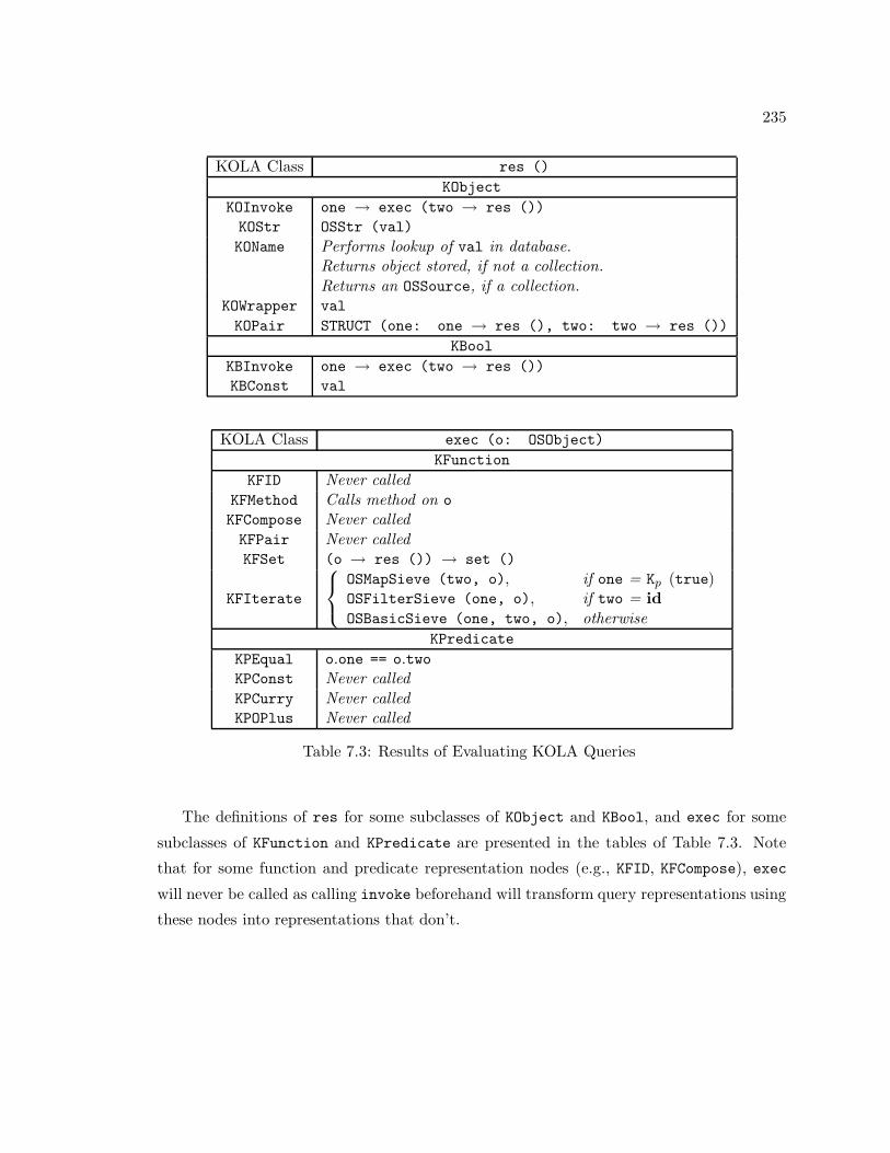
235
KOLA Class res ()KObject
KOInvoke one → exec (two → res ())KOStr OSStr (val)KOName Performs lookup of val in database.
Returns object stored, if not a collection.Returns an OSSource, if a collection.
KOWrapper valKOPair STRUCT (one: one → res (), two: two → res ())
KBoolKBInvoke one → exec (two → res ())KBConst val
KOLA Class exec (o: OSObject)KFunction
KFID Never calledKFMethod Calls method on oKFCompose Never calledKFPair Never calledKFSet (o → res ()) → set ()
KFIterate
OSMapSieve (two, o), if one = Kp (true)OSFilterSieve (one, o), if two = idOSBasicSieve (one, two, o), otherwise
KPredicateKPEqual o.one == o.twoKPConst Never calledKPCurry Never calledKPOPlus Never called
Table 7.3: Results of Evaluating KOLA Queries
The definitions of res for some subclasses of KObject and KBool, and exec for some
subclasses of KFunction and KPredicate are presented in the tables of Table 7.3. Note
that for some function and predicate representation nodes (e.g., KFID, KFCompose), exec
will never be called as calling invoke beforehand will transform query representations using
these nodes into representations that don’t.

236
NSFk = iterate (p, f) ! Bills such that
p = Cp (eq, ‘‘NSF’’) ⊕ topic,f = 〈name, set ◦ iterate (Kp (true), lgst cit ◦ reps) ◦ spons〉
Figure 7.4: NSF2k: The KOLA Translation of Query NSF2 of Figure 2.6
7.2 Putting It All Together: The NSF Query
We illustrate our design by tracing the processing of the KOLA version of NSF2 (NSF2k)
shown in Figure 7.4. Figure 7.5 illustrates the parse tree representation of this query over
which query evaluation takes place via successive calls of obj and res.
7.2.1 Initial Rewriting and Evaluation
For query NSF2k, there is little query rewriting or partial evaluation that can be performed
until data is touched. Calling obj on the parse tree representation of this query returns the
parse tree untouched. A subsequent call of res returns an OSBasicSieve with
• the parse tree representation of (Cp (eq, ‘‘NSF’’) ⊕ topic) as its predicate, p,
• the parse tree representation of
〈name, set ◦ iterate (Kp (true), lgst cit ◦ reps) ◦ spons〉
as its function, f , and
• The iterator object for Bills (i.e., an OSSource object) as its inner iterator, i.
This result is illustrated in Figure 7.6. In this figure and in others that include both KOLA
and ObjectStore objects, the two are differentiated by their shape: KOLA objects are drawn
with circles while ObjectStore objects are drawn with rectangles.
7.2.2 Dynamic Query Rewriting: Extracting Elements from the Result
The only query rewriting performed on NSF2k occurs when objects are retrieved from
the query’s iterator result. That is, rewriting occurs dynamically as a result of a call of
next on the OSBasicSieve of Figure 7.6. A call of next on this iterator in turn calls
next on the OSSource iterator for Bills. With each bill b returned by this call, a new
KOLA expression is formulated using the predicate (p) associated with the OSBasicSieve.

237
The formulated expression packages p with a predicate invocation node (KBInvoke) and
the KOLA translation of b (KOWrapper (b)) to construct the parse tree representation of
(p ? JbK) (such that JbK denotes the KOLA wrapper object referencing b). This is illustrated
in Figure 7.7 (A). Figure 7.7 (B) shows the result of calling obj on this tree. Figure 7.7 (C)
shows the result of calling res on the KOLA pair that is an argument to the predicate, eq.
(Evaluation then proceeds by comparing the one and two fields of the struct in (C).)
A trace of the calls of obj and res that lead to each result illustrated in Figure 7.7 is
presented below. Each step in the trace shows the “current” representation and the method
that was invoked most recently to generate it.
((Cp (eq, ‘‘NSF’’) ⊕ topic) ? JbK) → obj ()
= (Cp (eq, ‘‘NSF’’) ⊕ topic) → invoke (JbK → obj ()) (by KBInvoke :: obj)
= (Cp (eq, ‘‘NSF’’) ⊕ topic) → invoke (JbK) (by KOWrapper :: obj)
= Cp (eq, ‘‘NSF’’) → invoke (topic → invoke (JbK)) (by KPOPlus :: invoke)
= Cp (eq, ‘‘NSF’’) → invoke (topic ! JbK) (by KFAttr :: invoke)
= eq → invoke ([‘‘NSF’’, topic ! JbK]) (by KPCurry :: invoke)
= eq ? [‘‘NSF’’, topic ! JbK] (by KPEqual :: invoke)
Suppose that b is a House resolution. Calling res on
eq ? [‘‘NSF’’, topic ! JbK]leads to the comparison of the fields of the ObjectStore STRUCT of Figure 7.7 (C) as illus-
trated below.

238
(eq ? [‘‘NSF’’, topic ! JbK] → res ())
= eq → exec ([‘‘NSF’’, (topic ! JbK)] → res ()) (by KBInvoke :: res)
= eq → exec (STRUCT (one: ‘‘NSF’’ → res (), two: (topic ! JbK) → res ()))
(by KOPair : res)
= eq → exec (STRUCT (one: ‘‘NSF’’, two: (topic ! JbK) → res ()))
(by KOString :: res)
= eq → exec (STRUCT (one: ‘‘NSF’’, two: topic → exec (JbK → res ())))
(by KOInvoke :: res)
= eq → exec (STRUCT (one: ‘‘NSF’’, two: topic → exec (b)))
(by KOWrapper :: res)
= eq → exec (STRUCT (one: ‘‘NSF’’, two: b.topic)) (by KFAttr :: exec)
= ‘‘NSF’’ == b.topic (by KPEqual :: exec)
Suppose that b.topic == ‘‘NSF’’. Then this expression evaluates to true and b is packaged
with f to construct the query tree of Figure 7.8 (A), (〈name, set ◦ h ◦ spons〉 ! JbK), such
that
h = iterate (Kp (true), lgst cit ◦ reps).
Calling obj on this tree results in the query tree of Figure 7.8 (B) as is shown in the

239
execution trace below.
(〈name, set ◦ h ◦ spons〉 ! JbK) → obj ()
= 〈name, set ◦ h ◦ spons〉 → invoke (JbK → obj ()) (by KOInvoke :: obj)
= 〈name, set ◦ h ◦ spons〉 → invoke (JbK) (by KOWrapper :: obj)
= [name → invoke (JbK), (set ◦ h ◦ spons) → invoke (JbK)] (by KFPair :: invoke)
= [name ! JbK, (set ◦ h ◦ spons) → invoke (JbK)] (by KFAttr :: invoke)
= [name ! JbK, (set ◦ h) → invoke (spons → invoke (JbK))](by KFCompose :: invoke)
= [name ! JbK, (set ◦ h) → invoke (spons ! JbK)] (by KFAttr :: invoke)
= [name ! JbK, set → invoke (h → invoke (spons ! JbK))](by KFCompose :: invoke)
The next step of this reduction executes FIterate::invoke which fires a COKO trans-
formation to rewrite the query,
iterate (Kp (true), lgst cit ◦ reps) ! (spons ! JbK).Suppose that this rewriter has no effect on this query. Then the next step of the execution
trace is:
[name ! JbK, set → invoke (iterate (Kp (true), lgst cit ◦ reps) ! (spons ! JbK))].At this point, the COKO transformation associated with set is fired to rewrite the query,
set ! (iterate (Kp (true), lgst cit ◦ reps) ! (spons ! JbK)).If the COKO transformation is one that eliminates redundant duplicate elimination (firing
the rules of Figure 5.3), then the reduction continues as shown below:
1. Firing rule de1 of Figure 5.3 matches the pattern, set ! (iterate (p, f) ! A) with

240
the above query producing the variable bindings:
p = Kp (true)
f = lgst cit ◦ reps, and
A = spons ! JbK2. A Prolog query is issued to the Prolog interpreter to determine the truth values of
conditions:
is inj (lgst cit ◦ reps)
and
is set (spons ! JbK).The latter condition is satisfied by inference rule (2) of Figure 5.4b in combination
with schema information establishing the type of spons to return a set of House
Representatives. The former condition is satisfied by inference rules (2) and (3) of
Figure 5.4a in combination with metadata information identifying lgst cit as a key
for sets of regions, and reps as a key for sets of House Representatives.4
3. The success of the Prolog query leads to the firing of the conditional rewrite rule, de1,
leading to a rewrite of the query that performs duplicate elimination to one that does
not:
iterate (Kp (true), lgst cit ◦ reps) ! (spons ! JbK).Thus, the call of next on the OSBasicSieve of Figure 7.6 has led to a dynamic call
of the query rewriter to perform the semantic rewrite that eliminates redundant duplicate
elimination. The execution trace then concludes, producing the representation,
[name ! JbK, h ! (spons ! JbK)]such that
h = iterate (Kp (true), lgst cit ◦ reps).
4Our implementation resolves overloading (e.g., of attribute reps) by translating all references to functionsappearing in a schema, metadata files or queries to Prolog terms of the form,
fun (name, D, R)
such that name is the name of the function, D is the domain type of the function, and R is the range type ofthe function. Therefore, fun (kreps, kHouse Representative, kRegion) would be identified as a key andfun (kreps, kSenator, kRegion) would not be. A similar representation strategy is applied to predicates.

241
A call of res on this representation produces the result shown in Figure 7.8 (C) as is
illustrated by the execution trace below:
[name ! JbK, h] → res ()
= STRUCT (one: (name ! JbK) → res (), two: h ! (spons ! JbK) → res ())
(by KOPair :: res)
= STRUCT (one: name → exec (JbK → res ()), two: (h ! (spons ! JbK)) → res ())
(by KOInvoke :: res)
= STRUCT (one: name → exec (b), two: (h ! (spons ! JbK)) → res ())
(by KOWrapper :: res)
= STRUCT (one: b.name, two: (h ! (spons ! JbK)) → res ()) (by KFAttr :: exec)
= STRUCT (one: b.name, two: g → exec ((spons ! JbK) → res ()))
(by KOInvoke :: res)
= STRUCT (one: b.name, two: g → exec (spons → exec (JbK → res ())))
(by KOInvoke :: res)
= STRUCT (one: b.name, two: g → exec (spons → exec (b))) (by KOWrapper :: res).
Because the bill attribute spons returns a set, the result of the invocation,
spons → exec (b)
is an OSSource iterator (which will be expressed through the remainder of the trace as
“OSSource (b.spons)”. Therefore, the next expression in the execution trace becomes,
STRUCT (one: b.name, two: g → exec (OSSource (b.spons))).
Substituting for g, the expression labeled by two is:
iterate (Kp (true), lgst cit ◦ reps) → exec (OSSource (b.spons)).
Because the predicate argument to iterate is Kp (true), the call of KFIterate::exec
generates an OSMapSieve object, which will be written in the remainder of the trace as

242
“OSMapSieve (lgst cit ◦ reps, OSSource (b.spons))”. Therefore, the next expression in
the execution trace becomes,
STRUCT (one: b.name, two: OSMapSieve (lgst cit ◦ reps, OSSource (b.spons))).
The last step of the trace inserts the field names of the struct (bill and schools) that
appeared in the original OQL query and that are retained by translation into KOLA:
STRUCT (bill: b.name,
schools: OSMapSieve (lgst cit ◦ reps, OSSource (b.spons))).
7.2.3 Extracting Results from the Nested Query
The result of calling next on the OSBasicSieve of Figure 7.6 itself generates a record
(STRUCT) whose second value (schools) is another query operator. As elements from this
inner query result can also be extracted via calls to next, this makes it possible for the
query rewriter to be called deeply within evaluation. In this case, the function argument
of the OSMapSieve is simple enough that the rewriter is not called. A call of next on the
OSMapSieve initiates a call of next on the OSSource iterator over b.spons. The result of
this latter call (either a Senator or a House Representative, l) results in the formulation of
the expression,
(lgst cit ◦ reps) ! JlKwhose parse tree representation is illustrated in Figure 7.9 (A). A call of obj on this tree
generates the KOLA tree of Figure 7.9 (B) as shown below:
((lgst cit ◦ reps) ! JlK) → obj ()
= (lgst cit ◦ reps) → invoke (JlK → obj ()) (by KOInvoke :: obj)
= (lgst cit ◦ reps) → invoke (JlK) (by KOWrapper :: obj)
= lgst cit → invoke (reps → invoke (JlK)) (by KFCompose :: invoke)
= lgst cit → invoke (reps ! JlK) (by KFAttr :: invoke)
= lgst cit ! (reps ! JlK) (by KFAttr :: invoke).

243
KOInvoke
KFIterate KOName"Bills"
one two
one two
KPOPlus
KPCurry
KPEqual KOStr"NSF"
one
one
two
two
"topic"
KFPair
KFCompose
KFSet KFCompose
KFIterate
KPConst KFCompose
one
one
one
one
one one
two
two
two
two
two
KFAttr"spons"
"reps""lgst cit"KBConsttrue
KFAttr KFAttr
KFAttr"name"
KFAttr
Figure 7.5: The Parse Tree Representation of NSF2k

244
OSSource
OSBasicSieve
Bills
KPOPlus
KPCurry
KPEqual KOStr"NSF"
one
one
two
two
"topic"KFAttr
p
f
i
i
KFPair
KFCompose
KFSet KFCompose
KFIterate
KPConst KFCompose
one
one
one
one
one one
two
two
two
two
two
KFAttr"spons"
"reps""lgst cit"
KBConsttrue
KFAttr KFAttr
"name"KFAttr
Figure 7.6: The result of calling obj and res on the “NSF Query”

245
obj ()
res ()
KPOPlus
KPCurry
KPEqual KOStr
"NSF"
one
one
two
two
KBInvoke
KOWrapper
A
B
KPEqual
one two
KBInvoke
KOWrapper
KOPair
KOInvoke
one two
one
one
two
two
b
b
KFAttr"topic"
KOStr"NSF"
"topic"KFAttr
one two
"NSF"
struct
C
b.topic
Figure 7.7: Calling query NSF2k’s predicate on a bill, b

246
obj ()
res ()
one two
one
one
two
two
two
KOInvoke
KFPair
KFCompose
KFSet KFCompose
KFIterate
KPConst KFCompose
one
one
one
one
one one
two
two
two
two
two
KOWrapper
KOPair
KOInvoke
KFIterate
KPConst KFCompose
one
one
two
twoone
KOInvoke
KOWrapper
b
b
KFAttr"spons"
"reps""lgst cit"KBConsttrue
KBConsttrue
"lgst cit"
"spons"
KFAttr KFAttr
KFAttr
KFAttr"reps"
KFAttr
one
OSMapSieve
b.spons ()
struct
two
KFCompose
one two
"lgst cit""reps"
KFAttrKFAttr
OSSource
"name"KFAttr
one
twoKOInvoke
KOWrapper
"name"KFAttr
b
OSStrb.name
Figure 7.8: Calling NSF2f ’s data function on a House resolution, b

247
l.reps.lgst cit
KFCompose
onetwo
KOInvoke
KOWrapper
one two
KOInvoke
KOInvoke
one two
KOWrapper
obj ()
res ()
KFAttr"lgst cit" "reps"
"lgst cit"
"reps"
l
lKFAttr
KFAttr
KFAttr
Figure 7.9: Calling NSF2k’s inner query function on a House Representative, l

248
Calling res on this KOLA tree generates path expression
l.reps.lgst cit
as demonstrated below:
(lgst cit ! (reps ! JlK)) → res ()
= lgst cit → exec ((reps ! JlK) → res ()) (by KOInvoke :: res)
= lgst cit → exec (reps → exec (JlK → res ())) (by KOInvoke :: res)
= lgst cit → exec (reps → exec (l)) (by KOWrapper :: res)
= lgst cit → exec (l.reps) (by KFAttr :: exec)
= l.reps.lgst cit (by KFAttr :: exec)
7.3 Discussion
7.3.1 Cost Considerations
This chapter describes ongoing work and therefore inspires more questions than answers.
Dynamic query rewriting offers potentially enormous benefits for query evaluation given
that the wisdom or validity of some rewrites may depend on factors that cannot be de-
termined until run-time. In this chapter, we showed an example query (NSF2k) for which
dynamic query rewriting was beneficial. In processing this query, duplicate elimination
was avoided in many circumstances where it would have been required otherwise. If dupli-
cate elimination can be avoided multiple times in processing a query and avoided for large
collections, enormous savings in evaluation cost are likely.
On the other hand, dynamic query rewriting adds overhead to the cost of evaluating a
query. This cost arises because of the need to generate subplans during query evaluation.
For ad hoc querying (for which optimization and evaluation occur consecutively), this is
not an issue. But for queries that are compiled, an obvious question is whether or not the
costs of dynamic optimization outweigh its potential benefits.
Once our implementation is complete, this question will need to be addressed. But
there are reasons for optimism. First, dynamic query rewriting need not invoke the large

249
and expensive query rewrite routines that are likely to be invoked statically. Our present
design permits distinct COKO transformations to be associated with each KOLA query
operator. These rewriters could be quite simple, and perform only those rewrites that
offer large cost savings that justify the cost of dynamic rewriting. The rewrite to avoid
redundant duplicate elimination is one such example. The cost of the semantic reasoning
needed to decide whether duplicate elimination can be avoided is modest, but the potential
cost savings from avoiding duplicate elimination (especially for large collections) can be
enormous.
A second reason for optimism is that it may be possible to streamline the rewriting that
does occur dynamically. For example, memoization of the results of semantic queries could
greatly improve performance. Consider the example we presented in this chapter. For this
example, there are only two possibilities considered during semantic rewriting. Either a bill
is a House resolution for which duplicate elimination is avoidable, or it is a Senate resolution
for which duplicate elimination is required. Given the present design, the processing of each
bill results in one of two semantic queries being generated:
1. Is A a set given that it consists of sponsors of a House resolution, and is
lgst cit ◦ reps
injective given that it is a function over House Representatives?, or
2. Is A a set given that it consists of sponsors of a Senate resolution, and is
lgst cit ◦ reps
injective given that it is a function over Senators?
If the answers to these questions can be memoized when they are first answered, then
evaluation of semantic queries becomes trivial for all but the bills processed initially. In
fact, the use of a Prolog interpreter makes the implementation of memoization trivial. Prolog
facts (such as one that directly states that lgst cit ◦ reps is injective if reps ranges over
House Representatives) can be asserted as they are inferred.
The issues discussed in the Chapter 5 also are material here. Once our COKO compiler
generates more efficient code, and our semantic rewriter reasons directly over KOLA trees
instead of their Prolog interpretations, we believe that all rewrites (whether fired statically
or dynamically) will become more efficient.
Finally, dynamic query rewriting might be circumvented in some cases by allowing for
conditional plans (as in the Volcano dynamic optimization work of Graefe and Cole [25]).

250
Rather than deferring rewriting decisions until run-time, a conditional plan would statically
list multiple cases and associate plans to perform for each. Conditional plans could be useful
when the cases that will be considered dynamic query rewriter can be anticipated statically,
and when these cases are unlikely to change. We believe that dynamic query rewriting
should not be replaced by conditional plans in all cases because it can be hard to anticipate
all cases statically. For example, in this chapter we have shown that the subtype to which an
object belongs can be relevant to the choice of query evaluation strategy. New subtypes are
easily defined for object-oriented databases. Therefore, a conditional plan that is unaware
of changes to the schema can become obsolete.
7.3.2 The Advantage of KOLA
In previous chapters, we showed how KOLA’s combinator style facilitates the expression
of declarative rules. Term rewriting and semantic inference are similar in that both must
perform subexpression identification and query formulation. Expressed over KOLA queries,
neither of these tasks require supplemental code.
In this chapter, we have shown that subexpression identification and query formulation
have uses beyond the expression of a query rewrites. Dynamic query rewriting is query
rewriting that occurs during a query’s evaluation. Typically, dynamic query rewriting
requires a query evaluator to identify subexpressions of the query it is processing, and to
formulate new queries to dynamically submit to a query rewriter. We have shown that
the expression of these two tasks is simplified with the use of KOLA as the underlying
query representation. Therefore, dynamic query rewriting provides another example of how
KOLA benefits the development of query optimizers.
7.4 Chapter Summary
This chapter has described ongoing work in dynamic query rewriting. Query rewriting is
most effective when a rewriter has knowledge about the representations and contents of the
collections involved. Dynamic query rewriting is useful when this information is unavailable
until data is accessed, as in object-oriented databases, network databases and heterogeneous
databases.
We have confined our discussion in this chapter to potential benefits and design ap-
proaches for dynamic query rewriting over object-oriented databases. We showed an object-
oriented query (NSF2k) that could be evaluated efficiently with dynamic query rewriting.

251
Specifically, dynamic query rewriting makes it possible to evaluate this query without hav-
ing to perform duplicate elimination as many times as would be required otherwise. We
described the design of a dynamic query rewriter for ObjectStore for which an implemention
is under development. While the work in this area is incomplete, the ideas demonstrate an
exciting direction for query processing enabled by a combinator representation of queries.
Chapter 8
Related Work
In this chapter, we consider work related to the work presented in this thesis. The chapter is
divided into four sections that correspond to Chapters 3 (KOLA), 4 (COKO), 5 (Semantic
Query Rewriting) and 7 (Dynamic Query Rewriting) respectively.
8.1 KOLA
KOLA is both a query algebra and an internal data structure for query optimizers. The
association of data structure with algebra is deliberate, and reflects our goal of simplifying
both the operation and verification of query rewriting.
The best known query algebra is the relational algebra of Codd [24]. While used to de-
scribe logical query rewrites in many database texts (e.g., [66], [80]), the relational algebra
is not usually used as a data structure within query optimizer implementations.1 The Star-
burst query rewriter [79] for example, uses the Query Graph Model (QGM) as its internal
representation. QGM query representations resemble instances of the entity-relationship
data model. The entities (vertices) for this model are collections such as stored tables or
queries. Edges reveal relationships between collections that indicate that one is an input to
the other (the other being a query), or that a correlated predicate compares elements from
each.
Starburst query rewrite rules are written in C. In [79], it is argued that it is necessary
to code rules in this way because QGM is a C data structure. We dispute this conclu-
sion — rules could be expressed more declaratively and a compiler could generate C code1Although Microsoft’s SQL Server does use a variation of the relational algebra in this way.
252

253
from these more abstract specifications. (For example, KOLA’s data structures are imple-
mented in C++ and COKO transformations and KOLA rewrite rules are compiled into
C++ code.) Instead, we believe that code is necessary to specify Starburst rules because
the close association between QGM and SQL makes QGM a variable-based representation.
8.1.1 KOLA and Query Algebras
KOLA joins the numerous object query algebras that have been proposed over the years,
including AQUA [70], EQUAL [87], EXTRA [99], OFL [40], GOM [61], Revelation [98],
LERA [35], ADL [91], and the unnamed algebra of Beeri and Kornatzky [7]. Despite the
lack of a standard, there is an encouraging overlap in the operators found in all of these
algebras. These operators include:
• generalizations of relational operators (e.g., (1) a mapping operator generalizing rela-
tional projection by mapping a function over all members of a collection, (2) a selection
operator generalizing relational selection by selecting elements of a collection satisfy-
ing a given predicate, and (3) a join operator generalizing relational joins by relating
elements drawn from multiple collections),
• aggregation operators (such as the fold operator of AQUA [70] and Revelation [98])
that give algebras expressive equivalence with standard query languages with opera-
tors such as SUM and COUNT, and
• conversion operators to convert back and forth between flat and non-flat collections
(including a grouping or nesting operator to convert a flat collection to a non-flat
collection, and a flattening or unnesting operator to flatten a non-flat collection).
KOLA defines operators in each of the above categories. Mapping and selection are cap-
tured by KOLA’s iterate and iter formers. Joins are expressed by a number of query
primitives and formers, including join, lsjoin, rsjoin and int. Grouping is captured by
njoin. Collection flattening is captured by unnest and flat. Thus, KOLA is equivalent
in spirit to other object query algebras. The uniqueness of KOLA is in form — KOLA is
a combinator-based representation specifically designed to simplify the operation and the
verification of the query rewriter.
The KOLA Heritage – The AQUA Family of Query Algebras: The direct ances-
tors of KOLA are AQUA [70], EQUAL [87], EXTRA [99] and Revelation [98]. AQUA [70]
was the immediate predecessor to KOLA. (KOLA was defined in response to difficulties

254
defining a formal specification for AQUA and expressing rewrite rules over AQUA queries.)
AQUA was designed by the inventors of EQUAL [87], EXCESS [99] and Revelation [98] who
attempted to integrate and reconcile the approaches taken with their predecessor algebras.
AQUA defines a very general set of query operators, each of which can be instantiated
with any data function or data predicate. For example, AQUA’s join operator can be
instantiated with a tuple concatenation function to express a relational join, or with a
function that uses a query operator to express a join over an object-oriented database. This
approach to query operators influenced the design of KOLA’s query formers.
Aside from its combinator style, KOLA’s primary distinction from AQUA concerns
how it integrates data and query functions and how it constrains the definition of equality
predicates. In AQUA, data functions are defined as lambda expressions whereas query
functions are not. In KOLA, all functions are defined uniformly. This approach simplifies
query formulation which need not massage query functions to make them data functions or
vice-versa. This is especially important in an object query algebra where the pervasiveness
of nesting means that query functions are often used as data functions.
AQUA allows arbitrary equivalence relations to act as equality predicates. Query op-
erators whose semantics depend on equality definitions (such as set and bag union) are
defined with equality predicate paramaters so that the semantics of these operators can
be configured according to their intended use. KOLA demands that equality definitions
be confluences (as in CLU [72]): predicates that determine two objects to be equal only
if they are indistinguishable. For mutable object types, equality predicates must compare
immutable object identifiers. For immutable object types, equality predicates must be keys.
KOLA has a more rigid policy with respect to equality predicates because substituting ar-
bitrary equivalence relations for equality predicates can result in unintuitive query results.
For example, a query that is instantiated with a non-confluent equality predicate can be is-
sued twice over the same data and return two collections with distinct cardinalities (making
these collections unequal by any reasonable interpretation of equality). As well, equality
definitions that determine two distinct objects to be equal (perhaps because at the time
of comparison, their states were identical) can result in a collection whose cardinality can
change as a result of mutating one of its elements. These issues are discussed at length in
our DBPL ’95 paper [23].
OFL: Like KOLA, OFL [40] is inspired by functional programming languages [34]. OFL
is an algebra intended to simplify the generation of graph representations of queries. The
strategy taken to evaluate the query varies according to how this graph representation is

255
traversed.
OFL is an alternative intermediate representation to parse structures of standard ob-
ject algebras. These algebras, it is argued, unnecessarily constrain the choice of execution
algorithms. For example, the algebraic representation of path expressions demands eval-
uation by an inefficient object-at-a-time navigation. On the other hand, the graph-based
representation espoused by this work enables the same query to be mapped to a plan that
evaluates the query using joins. This then is an alternative approach to solving the nor-
malization problem addressed by query rewriting. The usual example used to motivate
query rewriting involves nested queries that force optimizers to choose nested loop evalua-
tion strategies. Rewriting transforms nested queries into equivalent join queries that offer
optimizers more algorithmic choice. In Chapter 6, we showed how query rewriting could
also normalize queries with path expressions to ensure the consideration of evaluation plans
involving joins.
The OFL language consists of both functional and imperative constructs (such as a
sequencing operator). The imperative flavor makes OFL more of a plan language than an
algebra, as algebraic equivalences are hard to establish and verify when expressions are
described by the algorithms that generate them. But we find the alternative to query
rewriting proposed by this work intriguing. In short, this approach generates multiple
evaluation alternatives by fixing, rather than rewriting, a query’s representation and instead
varying traversal orders over it. Therefore OFL has some commonality with COKO which
is also concerned about the order in which a given query representation is visited, though
in the context of rewriting rather than evaluation.
LERA, GOM and ADL: Object query algebras LERA [35, 36], ADL [91] and GOM [61]
are generalizations of the relational algebra. All of these algebras support tuple operators
such as tuple concatenation (used in joins, unnests and nests). The KOLA data model
includes pairs rather than tuples because the fixed number of fields in a pair simplifies
its formal specification. Translation of OQL queries into KOLA maps tuples (structs)
into (nested) pairs with tuple references replaced by compositions of projections that make
appropriate extractions. (Our translator implementation keeps track of field names so that
KOLA pair results can be translated back into tuples before they are stored.)
Like KOLA, LERA avoids direct references to variables within queries. But rather
then using a combinator notation, LERA uses a numbering scheme to replace a variable
reference with an index indicating the collection over which the variable ranges. Therefore,
LERA’s scheme is similar to the deBruijn [30] scheme (see Chapter 6), but is static. That

256
is, collections appearing in a query are numbered from left to right rather than according
to their relative positions within environments. The purpose of this notation is to avoid
ambiguity (e.g., if the same collection appears twice in a join). With respect to rewrite
rules, this approach still suffers from the same problems that make rewrite rules over query
expressions require code. In particular, subexpression identification over such expressions
requires code because a variable’s index does not indicate whether or not it is free. As
well, query formulation requires code because a variable index may have to be adjusted if
rewriting results in changes to the collections that appear in a query’s FROM clause (e.g., as
in a nested query → join query normalization).
GOM [61] and ADL [91] contain semijoin and nested join operators that inspired equiv-
alent operators in KOLA. Specifically, KOLA’s njoin former was inspired by ADL’s njoin
and GOM’s djoin operators. ADL also defines semijoin and antijoin operators that are
semantically equivalent to instantiations of KOLA’s left semi-join former. (The function,
lsjoin (ex (p), id)
is equivalent to ADL’s semijoin operator with respect to predicate p, and
lsjoin (fa (∼ (p)), id)
is equivalent to ADL’s antijoin operator with respect to predicate p.) GOM defines a left
outer join operator that performs a union on the result of these two functions, but applying
different functions (f and g) to the results of the semijoin and antijoin. Left outer-joins are
also expressible in KOLA. For any pair of collections A and B, the left outer-join of A with
respect to B is:
uni ! [lsjoin (ex (p), f) ! [A, B], lsjoin (fa (∼ (p)), g) ! [A, B]].
8.1.2 KOLA and Combinators
KOLA’s combinator style was inspired by Backus’ functional language, FP. Like FP, KOLA
was initially intended to be a user-level language. But we abandoned this approach when
it became clear that combinators make languages difficult for users to use.
The use of combinators as internal representations of functional programs originated
with Turner’s seminal work [93]. Ever since, combinators have been used within strict
functional language compilers (e.g., Miranda [94]) as internal representations of lambda
expressions. The use of combinators in this way makes evaluation by graph reduction more
efficient, as lambda expressions with free variables force unnecessary copying of potentially

257
large function bodies [34]. Approaches to combinator translations can be classified according
to whether the combinator set is fixed or variable. Fixed combinator sets consist of a finite set
of combinators that are used as the target for all lambda expression translations. The best
known of the fixed sets of combinators is the SKI combinator set introduced by Schonfinkel
[82]. It has been shown that this small set is sufficient to translate all of the lambda calculus
(in fact I is superfluous), but the size of the resulting code is too large to be of practical use
[57]. Variations of the SKI combinator sets add additional, redundant combinators (e.g. B
and Y) to reduce the size of the translated code. Curien [27] proposed a set of combinators
inspired by Category Theory, which he used to provide an alternative semantics for the
lambda calculus. Of all of the combinator translations we found described in the literature,
KOLA most closely resembles Curien’s combinator set, but adjusted to account for sets and
bags rather than lists, and avoiding the overly powerful combinators (App and Λ) that are
expressive but difficult to optimize prior to their application to arguments.
Lambda lifting [56] and supercombinators [52] are translation techniques that use vari-
able sets of combinators. These techniques construct new combinators during each trans-
lation. The goal of this technique is to keep the number of combinators in the result small
(the combinators generated tend to be fairly complicated). Thus, the goal of removing
free variables from lambda expressions is achieved without an explosion in the size of the
resulting code.
Despite the wide-spread use of supercombinators in functional language compilers, we
settled on a fixed set of combinators for KOLA for the following reasons:
• query optimization (which relies on a set of known rewrite rules) must reference a
known (i.e., fixed) set of operators, and
• query optimization can tolerate query representations that are larger (within reason)
than queries because queries tend to be small compared with functional programs.
KOLA is not the first combinator query algebra or query language. ADAPLAN [31]
was proposed as a combinator-style query language, but combinators are difficult for users
to master and ill-suited as query languages. FQL [12], NRL [10] and the unnamed algebra
of Beeri and Kornatzky [7] are combinator-based query algebras. FQL was an early effort
and limited to relational databases. The algebra of Beeri and Kornatzky and NRL are
mathematical formalisms rather than optimizer data structures. That is, the purpose of
both of these algebras is to simplify the correctness of rules expressing query rewrites. Both
algebras are minimal in that they include no redundant operators. A minimal algebra

258
simplifies proof obligations, but is less effective as an optimizer data structure. Redundant
operators (such as join operators) are necessary in optimizer implementations because they
are highly suggestive of the kinds of algorithms that a plan generator should consider. This
redundancy is exactly what query rewriting normalizations exploit — rewriting queries into
alternative forms that use operators to suggest alternative evaluation strategies.
8.1.3 KOLA and Query Calculii
A query calculus differs from a query algebra in that it specifies a query in a more declar-
ative way (i.e., by describing the result of the query rather than the sequence of operators
that generate it). The declarative flavor of query expressions can make it easier for a plan
generator to generate multiple execution plans, and therefore calculus-based query represen-
tations have advantages over query algebras for which plan generation is more constrained.
Put another way, the translation of queries into a declarative calculus is another way to
achieve the normalization goal of query rewriting. But the declarative nature of query cal-
culii makes it difficult to express heuristics that are easily expressed over a query algebra.
For example, it is not clear how one would express a rewrite that reorders filter predicates
over queries with a calculus-based representation.
As was the case for algebras, a standard for object query calculii has yet to emerge.
But perhaps the most common calculus for object queries stems from the monoid homo-
morphism work of Tannen et al [9]. That work describes structural recursion: a simple
and highly expressive formalism for specifying both queries and data types, but requiring
that functional inputs to homomorphisms satisfy certain undecidable algebraic properties
(commutativity, associativity and idempotence). Later work from this group [10] proposed
specific instantiations of these homomorphisms that were known to satisfy these properties
(e.g., instantiations with set union), but at the expense of expressivity. Further, while en-
suring a clean mathematics the idempotence restriction makes it difficult to express certain
query operations such as aggregations. For example, SQL’s SUM operator cannot be simu-
lated with a homomorphism instantiated with addition (‘+’), because ‘+’ is not idempotent.
The Monoid Comprehension calculus of Fegaras and Maier [33] is defined in terms of
monoid homomorphisms, but restricts the homomorphisms that can be expressed. In this
way, the problem of deciding algebraic properties of functions is avoided, as are other
problems inherent in the structural recursion model such as whether or not a given monoid
homomorphism instantiation can be evaluated in polynomial time. (All queries expressed
in the Monoid Comprehension calculus can be evaluated in polynomial time.) We consider

259
the Monoid Comprehension calculus to be complementary to object query algebras such as
KOLA, much as the relational calculus is complementary to the relational algebra. However,
unlike the relational calculus and algebra, the Monoid Comprehension calculus is not able
to express certain operators found in most object algebras. For example, operators based on
OQL’s bag intersection and bag difference operators cannot be expressed as homomorphisms
and are therefore inexpressible in the Monoid Comprehension calculus.
8.2 COKO
In Chapter 4, we introduced a language (COKO) for expressing complex query rewrites.
Other rule-based systems express complex query rewrites in one of two ways:
• as individual rewrite rules (usually supplemented with code), or
• as groups of rules.
8.2.1 Systems that Express Complex Query Rewrites With Single Rules
Most rule-based systems express complex query rewrites with individual rules. However, the
rules of these systems are not declarative rewrite rules that get fired by pattern matching.
Some systems (e.g., Exodus/Volcano [13, 43], EDS [36] and OGL [84]) allow rewrite rules
to be supplemented with code. Other systems (e.g., Starburst [79], and Opt++ [58]) allow
rules to be expressed completely in code, thus avoiding pattern matching altogether. Still
other systems (e.g., OGL [84] and Gral [6]) employ a variation of pattern matching to make
its effects more drastic. One rule-based optimizer generator (Cascades [42]) does all of these
things.
Starburst: Starburst [79] fires production rules (as in expert systems such as [11]) during
query rewriting. These rules consist of two code routines (loosely corresponding to the head
and body patterns of a rewrite rule) that are both written in C. Because they are written in
C, Starburst’s query rewrite rules can express a wide variety of transformations including
view merging, nested query unnesting (both discussed in [79]) and magic sets transforma-
tions ([74, 86]). However, Starburst rules are difficult to understand and verify, requiring a
detailed understanding of the underlying graph-based query representation (QGM).
Opt++ and Epoq: Opt++ [58] is not a rule-based system per se, but does permit
the modular expression of query rewrites. Opt++ is a C++-based framework for the

260
development of optimizers. This framework includes a family of classes from which optimizer
developers can inherit. One of these classes (Tree2Tree) defines objects that transform
tree representations of queries. Query rewrite rules would be implemented as instances of
subclasses of Tree2Tree. Thus, rules in this system would be code-based. Epoq [73] also
defines a framework for building optimizers. The modules for this framework (regions) are
special purpose optimizers that may or may not be rule-based. Epoq is intended to be
flexible enough to support any conception of rule including those defined with code.
Exodus/Volcano/Cascades: Exodus [13] and its successors, Volcano [43] and Cascades
[42] use rules that resemble rewrite rules, but that can have code supplements. Cascades
goes so far as to allow rewrite rules to be replaced by code altogether (such rules are called
“function rules”2). Cascades also uses a variation on pattern matching. (Cascade rules fire
fire on sets of query expressions and returns sets of modified query expressions as a result.)
Complex rewrites not expressible in this way would have to be expressed with function
rules.
EDS and OGL: Like the Exodus family of optimizer generators, EDS [36] and OGL [84]
permit code supplements to rules. EDS rules can have the form,
if <term0> under <constraint> then execute <method list> rewrite <term1 >
such that term0 is a head pattern, term1 is a tail pattern, and <constraint> and <method
list> contain calls to supplemental code written in C or C++. OGL rewrite rules can
include condition code (code supplements to head patterns) and can use meta-patterns
to circumvent standard pattern matching (e.g., “*V ” is a multivariable that “matches”
multiple terms at once). While multivariables make some rules more general (an example
shown in [84] demonstrates how a pattern with a multivariable could be reused to reassociate
a conjunction expression with any number of conjuncts), other rules that require separating
the terms that collectively matched the multivariable become inexpressible. In general, the
use of rewrite rules makes the rules of all of these systems simpler to understand and verify
than those that are expressed completely with code. However, the code supplements to
these rules which enhance their expressive power offset their gains in verifiability.
Gral: Of the rule-based systems we looked at, Gral [6] comes closest to ours in its effort
to make rules declarative by avoiding code. Gral also expands the expressive power of a2In fact, a Cascades paper [42] cites a query rewrite analagous to SNF of Chapter 4 as an example rewritethat would be encoded as a function rule.

261
rewrite rule, but not by adding code supplements as in Exodus of EDS. Instead, Gral uses a
variation of pattern matching to recognize rules that have multiple tail patterns. Each tail
pattern of a rule is associated with a declarative condition on the queried data. A query
that matches a head pattern and satisfies some set of conditions is then rewritten according
to the associated tail pattern.
The conditions associated with tail patterns analyze the data that is queried such as its
representation, the existence of indices, cardinality etc. Therefore, Gral rules have expres-
sive power above and beyond traditional rewrite rules because they incorporate semantic
reasoning into the decision as to whether or not to fire a rule. But a Gral rule resembles a
conditional rewrite rule in KOLA rather than a COKO transformation. While useful for ex-
pressing semantic rewrites, such rules cannot express the traversal strategies and controlled
rule firing that a complex query rewrite requires. Instead, such rewrites must be expressed
using the Gral meta-rule language as discussed below.
8.2.2 Systems that Express Complex Query Rewrites With Rule Groups
Many systems (e.g., Starburst [79], Gral [6], EDS [36], GOM [61] and OGL [84]) provide
some form of meta-control language for rules that includes rule grouping and sometimes
sequencing. Rule groups can be associated with search strategies that indicate how the rules
in a group should be fired.
It is tempting to view COKO as a meta-rule language in this style, and to compare
COKO transformations with rule groups and firing algorithms with search strategies and
sequencing control. But this analogy is misleading. Firstly, the “rules” that are grouped by
these systems are more analagous to COKO transformations than KOLA rules. Secondly,
the purpose of rule grouping in these systems is to control the search for a “best” (according
to some cost model) alternative to a given query expression. Typically, rules in a rule group
will be fired on a query (or set of queries) exhaustively,3 with each successful firing generating
a new candidate query expression. The set of all candidate query expressions is then pruned
for those that are considered to be efficient to evaluate. This approach reflects a competitive
use for rule grouping – group all rules that contribute to some cost-based objective and let
the best sequence of rule firings reveal itself through attrition.
Given the competitive model, an exhaustive approach to firing is guaranteed to find an
optimal expression relative to some cost-model. Therefore, all of these systems allow rule3Exhaustive firing of rule groups resembles exhaustive firing of individual rules — every rule in the rulegroup is fired on every subexpression on the query repeatedly until rule firing no longer has any effect.

262
firing to be exhaustive, though many also provide other competitive strategies that are more
efficient than exhaustive searches. For example, EDS allows a parameter to be set that limits
the number of rule firing passes made of a query. Other systems provide pruning strategies
so that only some alternatives are generated (e.g, OGL provide search strategies such as
branch-and-bound and simulated annealing). Other systems permit rules (Starburst, GOM
and Exodus) or algebraic operators (Gral) to be ranked to help the optimizer decide which
rule to fire next thereby reducing the likelihood that poor alternatives are generated.
The purpose of rule grouping in COKO is not to generate alternatives but to modularize
the expression of a complex query rewrite. Rules are fired cooperatively rather than com-
petetively, and according to a firing algorithm tailored to a specific set of rules, rather than
to a search strategy that is defined independently. There is no search involved. Rewriting
is blind to the data and is concerned with the syntax of the result rather than its expected
cost. Therefore, firing algorithms operate differently from search strategies. Of the search
strategies listed above, the exhaustive strategy can work as a firing algorithm, but only
in restricted cases (rewrite rules must form a confluent set) and usually sacrificing perfor-
mance in the process (as with CNF). Firing algorithms needn’t be generic nor exhaustive
and instead can be customized to specific, fixed sets of rules. By avoiding exhaustive firing
in these cases, rewriting is made more efficient.
In short, rule grouping can be either competitive and cooperative. Competitive rule
grouping is supported by many existing rule-based systems, and is complementary to COKO
which simply provides a means of specifying the rules that are to be grouped. Cooperative
rule grouping is unique to COKO and is a technique for defining complex query rewrites
that are efficient to fire and verifiable with a theorem prover.
8.2.3 Theorem Provers
Whereas KOLA was designed to enable query rewrites to be verified with LP, COKO was
inspired by the use of LP itself. As we showed in Chapter 3, LP proofs are accompanied
by proof scripts that tell the theorem prover how to complete the proof.4 Proof scripts
resemble handwritten proofs, except that proof methods are interpreted operationally to
make the proof executable.
In many ways, a COKO transformation resembles a theorem prover proof script. Both
query rewrite and proof rely on the existence of some set of simpler rewrite rules (derived4Scripts with similar purposes are found in other theorem provers. For example, tacticals in Isabelle [78]are analagous to LP proof scripts.

263
from specification axioms in the case of proofs). In some cases, exhaustive firing of these
rewrite rules would complete the rewrite or proof. But in other cases, this could lead to
nonterminating derivations and in most cases, the rewrite and proof could be performed
more efficiently. Both proof script and COKO transformation control when rewrite rules
get fired to ensure efficient rewriting and ensure termination.
That having been said, there are of course many differences between LP and COKO.
LP includes instructions that correspond to proof techniques such as induction, contradic-
tion and proof by cases. COKO “proofs” are far more straightforward, requiring only the
rewriting of terms through successive rule firings. There is no need to rewrite the same
term to the same result multiple times with different sets of rewrite rules as is done when
an LP proof proceeds by cases or induction. There is no need find inconsistencies in an
augmented set of rewrite rules as is done when an LP proof proceeds by contradiction. But
COKO provides fine-gained control of rule firing not provided with LP by controlling the
order and the subtrees on which rules are fired. This form of firing control ensures that a
COKO rewrite is efficient compared to a theorem prover, which would be far too slow to
be a query rewriter.
8.3 Semantic Query Rewriting
Related work in semantic query rewriting and semantic query optimization5 either describes
specific semantic optimization strategies, or describes frameworks within which strategies
can be expressed.
8.3.1 Semantic Optimization Strategies
Most semantic optimization strategies exploit knowledge of integrity constraints. Integrity
constraints are assertions that get evaluated during database updates to guard against
data corruption. Because integrity constraints guard updates, they are constraints on data
values and are expressed primarily by describing data dependencies. For example, a domain
constraint ensures that specified columns have no values in common. Referential integrity
constraints ensure that values appearing in one column of a relation also appear as values
in a column of another relation. Functional dependency constraints ensure that tuples that
share values for some columns share values for other columns also.5The latter term is more commonly used in the literature.

264
The very early semantic optimization papers [48, 64, 15] propose rewrites that ex-
ploit knowledge about integrity constraints to generate alternative expressions of relational
queries. Hammer and Zdonik [48] use inclusion dependencies to substitute smaller collec-
tions for larger ones as inputs to queries (domain refinement). Many systems (such as
Starburst) use key dependencies to determine when duplicate elimination is unnecessary
(as described in Chapter 5). Predicate Move-Around [71] exploits knowledge of functional
dependencies to generate new filtering predicates for collections used as inputs to joins.
Order optimization [89] exploits functional dependencies to determine when sorting can be
performed early during evaluation or avoided altogether.
Semantic optimization strategies for object databases [1, 45, 16] exploit not only the
semantics of data (i.e., integrity constraints), but the semantics of the functions that appear
in queries as well. Aberer and Fischer [1] correctly point out that object query optimizers
require semantic capabilities to avoid (when possible) invoking expensive methods that
can dominate the cost of query processing. They suggest a number of ways that method
semantics can be expressed (e.g., by declaring that one chain of method calls equals another)
and used by rewrites over the queries that invoke them. The work of Chaudhuri and
Shim [16] and Grant et al. [45] also permit equivalent method expressions to be declared.
The latter work also supports the expresssion of more algebraic descriptions of functions
(e.g., that a function is monotonic). Beeri and Kornatzky [7] also define rewrites over
object queries that depend on algebraic conditions (such as the idempotence of a function).
KOLA’s semantic capabilities permit expression of integrity constraints as well as function
equivalences and algebraic properties of functions. KOLA’s uniqueness is in expressing
these properties in a manner that allows them to be inferred, and permitting the inference
of properties to be easily extended and verified.
8.3.2 Semantic Optimization Frameworks
As discussed in Chapter 5, the contribution of our work is not in presenting new semantic
query optimization strategies but in introducing a framework for their expression that their
ensures verifiability with a theorem prover. Optimization frameworks that incorporate
semantic query optimization strategies can be divided into three categories:
• Category 1: systems that support operator-specific rewrites,
• Category 2: systems that support conditional rewrites, and
• Category 3: systems that support both conditional rewrites and semantic inference.

265
As we move from the first to the third category, systems get more succinct in describing
semantic rewrites and hence more scalable. To illustrate, a category (1) system might
permit the expression of a rule such as
clip (blur (i)) →= blur (clip (i))
which says that the result of clipping a blurred image is the same as the result of blurring
a clipped image. (The latter is likely more efficient to perform given that blurring tends
to be an expensive operation, and clipping results in a smaller image to blur.) For other
functions that commute (e.g., an image inversion function (invert) and clip), a similar
rule would have to be defined:
clip (invert (i)) →= invert (clip (i)).
A category (2) system would permit the expression of the more general rule,
commutes (f, g) :: f(g(i)) →= g(f(i)),
which establishes that any functions f and g can be reordered provided that they commute,
and then permit metadata to identify pairs of commuting functions (e.g., commute (clip, blur)
and commute (clip, invert)). Category (2) systems provide a more succinct way to ex-
press a semantic rewrite because one rule can be defined to account for all commuting
functions, rather that one rule per pair of commuting functions as would be required in
a Category (1) system. This difference becomes even more pronounced if other rules are
defined that are also conditioned on the commutativity of pairs of functions. These rules
can use the same set of metadata facts used by the previous rule.
A category (3) system would allow the commutativity of pairs of functions to be in-
ferred. For example, a category (3) system might infer that a function f commutes with
a composition of functions, (g ◦ h) if f commutes with each of g and h. Category (3)
systems would allow a rewriter to infer that image clipping commutes with a function that
first blurs an image and then inverts it given that clip commutes with each of blur and
invert. A category (3) system is more succinct than a category (2) system at expressing
semantic rewrites, as a category (2) system would have to list all functions that commute
(including clip and (blur ◦ invert)). Below we consider related work in semantic query
optimization frameworks, classifying each in terms of these categories.

266
Category (1)
Chaudhuri and Shim’s work [16] involves optimizations of SQL queries that contain foreign
functions. They incorporate rewrite rules over foreign functions to express equivalent ex-
pressions. Each equivalence must be captured in a separate rule. These rules are always
valid, therefore they perform no inference nor conditional rewrites and fall under category
(1).
The work on E-ADT’s in the Predator Database System [88] also falls under category
(1). One of the goals of this work is to localize semantic optimizations to optimization
components that are responsible only for queries involving the associated abstract data
types. The rule facility defined for Predator demands that rules be operator-specific. But
in fairness, the primary contribution of Predator is architectural. There is no reason that
a category (3) semantic rewriting system could not be incorporated into their framework.
Schema-specific properties (e.g., establishing that reps is a key) could be localized to E-
ADT’s, and inference rules could be maintained globally.
Category (2)
Beeri and Kornatsky [7] present several rewrite rules that are conditioned on function prop-
erties. For example, several of their rules are conditioned on the idempotence of a function.
However, they do not define a mechanism to define how properties such as idempotence are
inferred. Therefore the semantic rewriting proposed in this work falls under category (2).
More recent work in the context of object models has looked at semantic rewriting in
the presence of methods. Aberer and Fischer [1] consider semantic rewrites that depend on
method equivalences, and predicate implications derived from method semantics. Method
equivalences are conditioned on the domain of free variables appearing within the expres-
sions, and are used to rewrite query expressions according to a fixed set of rules. For
example, an equivalence can establish that two functions, f(x) and g(x) are equivalent for
all x in some collection C. The system uses this equivalence to infer that mapping f over
C is equivalent to mapping g over C.
The work of Aberer and Fischer falls short of other category (2) systems because the
rewrites that can depend on semantic conditions are limited to those provided by the system.
Equivalence relationships are only used to rewrite queries involving mapping and selection.
Predicate implication (which resembles predicate strength) is used in a rule that rewrites
selections (presumably with expensive predicates) to natural joins of collections filtered with
the cheaper predicates. No other rewrites that exploit these conditions can be added, and

267
no other conditions can be defined.
Category (3)
Grant et al [45] propose a framework for semantic query optimization (SQO) by which object
queries expressed in query languages such as OQL get translated into Datalog for semantic
processing. Semantic information about the underlying object schema (e.g., subtyping
information and methods) get expressed as Datalog rules that infer new integrity constraints
to attach to these queries. Various checks are then made of the resulting predicates (e.g., to
see if the new predicates introduce inconsistencies thereby eliminating the need to evaluate
the query) before the Datalog queries are then translated back into the language in which
they were posed.
This work falls under category (3) because of the use of inference to generate new
integrity constraints. But the inference performed by SQO is less general in its application
than that performed by COKO. SQO performs inference to generate predicates that get
attached to queries. COKO properties can infer any condition that guards the firing of a
rewrite rule, and not just predicate strength. Moreover, inferred conditions can guard the
firing of any conditional rewrite rule, and not just a rule that adds weaker predicates to
existing predicates. Effectively, this rule is the only conditional rule invoked by SQO. Its
KOLA equivalent is captured by rewrite rule str2 of Figure 5.6.
SQO improves upon our work in its use of a more powerful inference technique (partial
subsumption) to generate new predicates. We are interested in studying this inference
technique to see if it could be used to strengthen our inference capabilities and thereby
make our semantic rewriting component a better approximation of a complete system.
In summary, related work in semantic query optimization describes strategies and/or
frameworks for expressing semantic query rewrites. Semantic optimizations for relational
queries primarily use integrity (i.e., data) constraints. Semantic optimizations for object
databases reason about the semantics of functions also. This is appropriate given that
functions appearing in object queries are not limited to trivial extractions of values from
columns, and can dominate the cost of evaluating the query.
Frameworks for semantic query optimization can be classified into three categories that
are successively more succinct in expressing classes of query rewrites. Systems in category
(1) permit the expression of operator-specific rewrites. Systems in category (2) permit the
expression of more general conditional rewrites. Systems in category (3) permit the expres-
sion of conditional rewrites and techniques for inferring the conditions that are not explicitly

268
stated. Our work is unique in how it captures data and function-based semantic rewrites
within a category (3) framework in a manner supporting extensibility and verification with
a theorem prover.
8.4 Dynamic Query Rewriting
In this section, we describe work related to our dynamic query rewriting work that is
ongoing and presented in Chapter 7. Because our work is ongoing, we do not yet have
experimental results to justify or refute our intuitions. Therefore, the comparisons made to
other work in the area are confined primarily to approach rather than to a relative analysis
of performance.
The dynamic query optimization strategies that have been proposed in the literature
have exclusively concerned plan generation. Dynamic plan generation defers the generation
of complete execution plans until cost-related factors can be observed at run-time. Such fac-
tors can include availability of resources [53], run-time values for host variables in embedded
queries [25], or selectivity estimations [5].
The systems discussed here differ primarily by when alternative plans are generated.
The first category of systems (described in Section 8.4.1) use dyanmic plan selection rather
than dynamic plan generation. That is, what these approaches have in common is that
compile-time optimization produces a fixed set of alternative plans from which a choice is
made at run-time. Work falling in this category includes the dynamic optimization work
for Volcano of Graefe and Cole [25], parametric query optimization [53] and the dynamic
optimization performed by Oracle RDB [5]. The second category of systems (described
in Section 8.4.2) perform adaptive query optimization. These systems generate complete
execution plans at compile-time but permit all or portions of these plans to be replaced
during query evaluation. Proposals in this category include the query scrambling work out
of the University of Maryland [4] and the mid-query reoptimization work for Paradise of
Kabra and DeWitt [59]. Dynamic query rewriting more closely resembles systems in the
latter category, but generating partial plans rather than complete plans at compile-time.
Dynamic query rewriting is closely related to partial evaluation [26], as it reduces
compile-time query optimization to partial plan generation. We consider this relationship
more fully in Section 8.4.3.

269
8.4.1 Dynamic Plan Selection
We classify systems that choose plans dynamically from a fixed set of alternatives generated
at compile-time as dynamic plan selection strategies. The work of Graefe and Ward [44] and
later, Graefe and Cole [25] for Volcano was among the first dynamic plan selection strategies
proposed. This work proposes a plan language that includes a choose-plan operator that
makes it possible to express conditional plans. All subplans appearing below a choose-plan
operator are alternative plans that compute the same result. The execution of this operator
performs a cost analysis at run-time to determine which of these alternative plans should
be executed.
Graefe and Cole rule out dynamic invocations of the query optimizer, arguing that the
overhead involved would offset the performace gains from dynamically generated plans.
This is undoubtedly true in certain cases, but ignores certain factors that make dynamic
calls to an optimizer (and rewriter) of potential benefit:
• It assumes that a call to a dynamic query optimizer is a call to the same query
optimizer that performed compile-time optimization. In fact, there is no reason not
to define more streamlined optimizers and rewriters specifically defined to perform
optimizations that are quick and most likely to have cost benefit (such as query
rewrites). This is the approach taken in Oracle RDB [5] (which has separate optimizer
components for their query compiler and query executor)
The Volcano solution can be viewed as dynamically invoking an optimizer that is as
streamlined as an optimizer can be, deciding between a fixed set of plans according
to a fixed set of metrics. We believe that the optimizers that are invoked dynamically
could fall anywhere on a complexity scale, depending on the costs of the optimizations
they perform and the potential benefits that they offer to the query being evaluated.
• The more sophistated the reasoning performed by a conditional Volcano plan (i.e.,
the more choose-plan operators that appear in the conditional plan) the larger the
generated plan will be. Large plans can end up using resources (e.g., buffer space)
that would otherwise be used in evaluating the query. Less sophisticated reasoning
will produce smaller plans but are less likely to be effective in general. No study is
made in [25] of the sizes of conditional plans and the impact of plan size on evaluation
performance.
In short, this work was pioneering in suggesting how to implement a limited form of
dynamic query optimization. But the results presented here can be generalized in two ways:

270
1. The complexity of the optimizer invoked dynamically can vary and not be just one
that chooses between a fixed set of plans on the basis of a fixed set of cost factors.
2. Dynamically invoked optimizers need not be cost-based plan generators/selectors but
could be heuristic-based query rewriters that perform semantic inference. In fact,
query rewrites typically involve far simpler reasoning than do plan generators and can
have far greater impact on performance. This makes them ideal as candidate dynamic
optimizations where the cost : benefits ratio is of utmost concern.
Oracle RDB [5] justifies the dynamic optimization it performs by noting that the reli-
ability of compile-time cost (specifically, selectivity) estimation degenerates quickly in the
presence of complex predicates (e.g. p AND q). The problem is that the commonly held
assumption of predicate independence (i.e., the assumption that the correlation between
p and q has value 0) is overly simplistic — in fact correlation between predicates can fall
anywhere between -1 (meaning that for all x, p(x) ⇒ ¬q(x)) and 1 (meaning that for all x,
p(x) ⇒ q(x)). When correlation factors are assumed to be non-zero, selectivity estimation
of complex predicates such as “p AND q” fall in a (Zipfean) distribution that is relatively
constant independent of the individual selectivities of p and q. Therefore, cost estimation
provides little guidance to the plan generator which is likely to generate the same plan
independently of selectivities associated with specific predicates appearing in the query.
The Oracle RDB optimization strategy chooses multiple plans that are ideal assuming
different selectivity scenarios. Evaluation then runs all of these plans in parallel for a short
period of time. Zipfean selectivity distributions make it likely that one of these plans will
produce a complete result quickly. Dynamic optimization chooses which of these multiple
plans to continue in the unlikely event that all plans fail to return a complete result in the
small window of time they were given to run.
This solution does not eliminate the need to make better compile-time cost estimations,
as these would eliminate the need to perform dynamic optimization and parallel plan exe-
cution in some cases (thereby reducing the evaluation overhead of the queries involved). We
are interested in determining if knowledge of underlying semantics might help in compile-
time cost estimations. For example, predicate strength inferences could potentially be
generalized to infer other correlation factors between predicates (predicate strength infers
only correlation factors of -1 or 1). Defining inference rules to infer correlation factors in
some cases would not be of use in our semantic rewrite scheme where semantic conditions
determine the validity of a rewrite. However, it is possible that inferences such as these
could be attached to query representations that are passed down to plan generation.

271
The goal of parametric query optimization [53] is to generate a plan-producing func-
tion as a result of optimizing a query. This function accepts a vector describing run-time
parameters (e.g., available buffers) and produces a plan customized to those conditions.
Compile-time optimization divides the k-dimensional space of run-time parameters (k is
the length of the vector) into partitions that share the same optimal plan. Run-time op-
timization finds the partition in which an input vector resides to determine the plan to
execute.
This work complements the work of Graefe and Cole [25] by demonstrating a technique
for deciding where choose-plan operators go in a conditional plan and how to generate the
plans from which a dynamic choice is made. As with [25], this work describes dynamic plan
selection rather than dynamic plan generation and says nothing about query rewriting.
8.4.2 Adaptive Query Optimization
Adaptive query optimization is distinct from dynamic plan selection in that it involves
generating and comparing alternative plans dynamically, and not just selecting from a fixed
set of plans generated at compile-time. Query scrambling [4] is one example of adaptive
query optimization. The context for this work is widely distributed databases (e.g., web
databases). Dynamic optimization is triggered in this setting by the unavailablity of queried
data sources. Specifically concerned with the orderings of multiple joins, query scrambling
dynamically alters a chosen join ordering when processing delays occur due to unavailable
data. This affects the plan generated at compile-time (the “join tree”) in two phases:
• Phase 1: During this phase, scrambling alters the traversal of the join tree (say from
a preorder traversal) so that intermediate results from other parts of the tree can be
generated.
• Phase 2: This phases makes changes to the join tree by reordering joins, so that
intermediate results can be generated from available data sources.
Kabra and DeWitt also propose a technique for reoptimizing queries during evalua-
tion [59]. Unlike query scrambling for which dynamic reoptimization is triggered by data
unavailability, reoptimization in this setting is triggered by recognition of errors in compile-
time cost estimates. An execution plan is generated at compile-time that is annotated with
the cost estimates used to generate the plan. Inserted at select positions in the plan are
instances of a plan operator that triggers statistical analysis (e.g., cardinality measures).
The execution of this plan then performs the indicated statistical analysis when these op-
erators are executed on the basis of data that has been processed. The costs measured at

272
this time are then compared to the statically estimated costs that annotate the tree. Then,
depending on factors such as the cost of the query, the error in static cost estimations and
so on, reoptimization may be initiated.
Both adaptive query optimization schemes described here differ from dynamic query
rewriting in that both involve the reoptimization of queries. That is, both of these ap-
proaches generate complete plans at compile-time and then dynamically replace these plans
as run-time circumstances warrant. On the other hand, dynamic query rewiting gener-
ates only partial plans at compile-time, leaving the holes in these plans to fill at run-time.
Thus, the goal of dynamic query rewriting is not to reoptimize but to delay optimization.
This approach is appropriate in the context of rewriting, which applies heuristics that are
independent of physical properties of the environment and underlying database. That is,
dynamic query rewriting is triggered, not by the recognition of cost factors that make cer-
tain evaluation strategies inappropriate, but by semantic properties of objects and functions
that make certain rewrites invalid.
In short, dynamic query optimization resembles dynamic query rewriting in that it in-
volves making decisions affecting evaluation strategies at run-time. But dynamic query op-
timization involves making cost-based decisions about evaluation plans at run-time, whereas
dynamic query rewriting involves heuristically rewriting query representations depending
on their validity established by identifying properties of objects recognized at run-time.
Rather than being competitive, in fact the two techniques are complementary — dynamic
query rewriting necessarily would precede dynamic query optimization.
8.4.3 Partial Evaluation
Partial evaluation is a technique for generating a program by specializing another with
respect to some of its inputs [26]. Essentially, the technique requires decoupling the control
flow of a program from its inputs. This can be done by unfolding, which replaces references
to expressions with the code that computes them (as in inlining) or by specializing, which
generates a program that has performed portions of the overall computation given knowledge
of certain inputs. Typically, specialization uses symbolic computation to partially evaluate
the expression computed by the more general program.
Partial evaluation techniques have been used in many areas of computer science including
compiler generation [55, 8] and pattern matching [65]. Recently, compiler technology has
adopted partial evaluation techniques to provide run-time code generation [69]. Dynamic
query optimization and dynamic query rewriting similarly incorporate partial evaluation

273
into code generation for queries.
Dynamic query rewriting and optimization necessitates that certain decisions about
plan generation be deferred until run-time. This transforms the static query rewriter and
optimizer into system components that produce partial results. If one looks at a generated
execution plan as a result of evaluation, then the partial plans generated by static optimizers
in this context are produced as a result of partial evaluation.6
On the other hand, dynamic query rewriting is in many ways the dual of partial evalua-
tion. The purpose of partial evaluation is to move certain steps of a run-time computation
(evaluation) into compile-time to achieve speed-up. But the purpose of dynamic query
rewriting is to move certain steps of a compile-time computation (query optimization) into
run-time to achieve greater flexibility. Note the essential difference here: query rewriting
is made no more efficient as a result of dynamic rewriting. The goal instead is for query
rewriting to be more flexible and therefore for the generated plans to be more efficient.
6Of the approaches described in this section, adaptive query optimization least resembles partial evalua-tion because static optimization produces a complete plan (and not a partial plan) that can get replaceddynamically.

Chapter 9
Conclusions and Future Work
Query optimizers are perhaps the most complex and error-prone components of databases.
The query rewriter is especially difficult to design and implement correctly. A query rewriter
is correct if it preserves the semantics of the queries it transforms. Errors in query rewriting
have been identified in both in research [63] and practice [41]. To this day, query rewriting
techniques are often published with handwaving correctness proofs or worse, without proofs
at all. This approach to correctness undermines confidence in the query processors that
incorporate these techniques.
This thesis addresses the correctness issue for query rewriting. Our goal was to build
query rewriters that could be verified with an automated theorem prover. Theorem provers
have been adopted by the software engineering community as tools for reasoning about
formal specifications and verifying implementations relative to those specifications. Com-
monly used for complex and safety-critical systems, query rewriting is yet another natural
application of this technology.
The key contribution of this thesis is to define methodologies and tools for meeting this
correctness goal. We have introduced COKO-KOLA: a novel framework for the specification
and generation of query rewrite rules for rule-based query rewriters. Query rewrite rules
generated within this framework are verifiable with the theorem prover LP. The foundation
of this work is KOLA, a combinator-based (i.e., variable-free) algebra and internal query
representation. Combinators are unintuitive to read and hence ill-suited as query languages.
However, combinators are ideal query representations for rule-based query rewriters because
combinator representations make it straightforward to declaratively (i.e., without code)
specify subexpression identification and query formulation. Subexpression identification
distinguishes the relevant subexpressions of queries that are being rewritten. Successful
274

275
identification of these subexpressions indicates that rewriting should proceed and defines a
bank of subexpressions that can be used during query formulation. Query formulation uses
identified subexpressions to construct new query expressions that are returned as the result
of rewriting.
Combinator representations make it possible to express subexpression identification and
query formulation with declarative rewrite rules that get fired according to standard pat-
tern matching. This is because combinator expressions, being variable free, contain no
occurences of free variables which can make syntactically identical expressions have distinct
semantics. Code supplements to rules are required when underlying representations are
variable-based. Supplements used for subexpression identification analyze the context of
identified subexpressions containing free variables. Supplements used for query formulation
massage identified subexpressions to ensure that their semantics are preserved when used
in new contexts. These code supplements are unnecessary when variables are removed from
the underlying query representation.
KOLA is a fully expressive object query algebra over sets and bags. It contains similar
operators as other object algebras, but differs from these algebras in its combinator founda-
tion and its uniform treatment of query and data functions. Because KOLA rewrite rules
are expressible without code supplements, they can be verified with an automated theorem
prover. We have verified several hundred KOLA rewrite rules with the theorem prover LP
[46]. The motivation for KOLA, its semantics and several examples of its use in expressing
queries and rewrite rules were presented in Chapter 3.
Rewrite rules are inherently simple. On the other hand, query rewrites can be complex.
Therefore, KOLA is insufficient for expressing many of the query rewrites that get used
in practice. In Chapters 4 and 5 we proposed techniques for expressing query rewrites
that are too general and too specific respectively, to be expressed as rewrite rules. Query
rewrites that are too general for rewrite rules include such complex normalizations as CNF
— a rewrite to convert query predicates into conjunctive normal form. CNF cannot be
expressed as a single rewrite rule because no pair of patterns is both general enough to
capture all expressions that can be rewritten into CNF (i.e., all Boolean expressions) and
specific enough to express their CNF equivalents. Put another way, any rewrite rule that
expresses a predicate and its CNF equivalent will not be general enough to successfully fire
on all predicates. To express complex and general rewrites such as this, we introduced the
language COKO in Chapter 4.
COKO transformations specify and generate complex query rewrites. Transformations
are both extensions and generalizations of KOLA rules. Transformations generalize KOLA

276
rules because they can be fired and succeed or fail as a result. Transformations extend
KOLA rules because they supplement sets of KOLA rewrite rules with a firing algorithm
that controls the manner in which they are fired. COKO’s firing algorithm language sup-
ports explicit control of rule firing, traversal control over query representation trees, con-
ditional rule firing, and selective firing over subtrees. COKO makes it possible to express
efficient query rewrites as we demonstrated in Chapter 4 with CNF. But while firing algo-
rithms control when and where rules get fired, only rewrite rule firings can modify query
representations. Therefore, COKO transformations are correct if the KOLA rewrite rules
they fire are correct, and by implication, COKO transformations can be verified with a
theorem prover. The motivation for COKO, the semantics of its firing algorithm language,
and several applications of COKO that rewrite query expressions into CNF or SNF, push
predicates, reorder joins and apply magic sets techniques were presented in Chapter 4.
In Chapter 5, we addressed an expressivity issue that is complementary to that addressed
by COKO. This issue concerns query rewrites that are too specific to be expressed as rewrite
rules. The validity of such rewrites depends on the semantics and not just the syntax of
the queries on which they are fired. To express such rewrites, we added conditional rewrite
rules and inference rules to COKO-KOLA. Conditional rewrite rules get fired like (uncon-
ditional) rewrite rules, except that identified subexpressions must also satisfy declaratively
expressed conditions. These conditions are specified with properties: collections of declar-
ative inference rules that our compiler compiles into code that gets executed during rule
firing. Both conditional rewrite rules and inference rules are expressed without code and
hence are verifiable with a theorem prover. The motivation and implementation of semantic
extensions to COKO-KOLA were presented with examples of their use in Chapter 5.
An example application of the COKO-KOLA framework was presented in Chapter 6. In
this chapter, we described and assessed our experience building a query rewriting component
for the San Francisco project of IBM. We learned from this experience that the COKO-
KOLA framework, while in need of refinement and an industrial strength implementation,
makes it possible to express “real” query rewrites succinctly and with confidence.
What is common to KOLA, COKO and the semantic extensions to COKO-KOLA is
the need to identify subexpressions and formulate new queries. KOLA’s conditional and
unconditional rewrite rules identify subexpressions and formulate new queries when they
successfully fire. COKO transformations must frequently identify subexpressions of queries
on which to fire rules (using the GIVEN statement). Inference rules identify subexpressions
of query expressions so that properties of these expressions can be inferred of the expres-
sions that contain them. We showed in Chapter 3 that combinators simplify the expression
277
of these tasks and make them verifiable with a theorem prover. Therefore, the high-level
contribution of this work is the recognition of the impact of query representations in general
and combinator-based representations in particular on the design, implementation and ver-
ification of a query optimizer. When built with combinators, query rewriters can be verified
with a theorem prover, thereby achieving the goal we set out at the onset to address the
inherent difficulty in building query rewriters correctly.
In Chapter 7, we identified another potential benefit of combinator-based query repre-
sentations. Whereas previous chapters considered how combinators simplify how rewrites
get expressed, in this chapter we showed how combinators could be used to change when
they get fired. Dynamic query rewriting proposes that some query rewriting take place
during the evaluation of a query. Dynamic query rewriting would be beneficial in settings
where the information that justifies the firing of a rewrite rules is unavailable until queried
data is retrieved. Such settings include object databases, whose queries may be invoked on
anonmymous embedded collections; network databases, whose queries may join collections
whose availabilitymay be unknown until runtime; and heterogenous databases whose queries
may reference collections that are represented with data structures known only to the local
databases they oversee. Dynamic query rewriting requires identifying relevant subqueries
and formulating new queries by packaging these subqueries with accessed data. Therefore,
dynamic query rewriting also benefits from combinator-based query representations.
9.1 Future Directions
Unlike the work presented in previous chapters, dynamic query rewriting is work in progress.
Therefore, future directions for this thesis work are primarily concentrated in this area. A
design for a dynamic query rewriter and query evaluator for ObjectStore [67] is complete
and an implementation is ongoing. Once complete, it will be necessary to run a performance
study to determine when (and if) the benefits of dynamic query rewriting outweigh its costs.
We plan to construct and populate the Thomas database described in Chapter 2 according
to the guidelines described in Section 7.1.1. Thereafter, a testbed of OQL queries will be
formulated to query this database. A variety of query rewriters will be generated using the
COKO compiler, varying in the degree and kinds of semantic and dynamic query rewriting
that each performs. That is, the COKO routines compared will include ones that:
• fire no rewrites,
• fire rewrites, but neither semantic nor dynamic rewrites,

278
• fire semantic but not dynamic rewrites, and
• fire both semantic and dynamic rewrites.
It should be straightforward to come up with examples (such as the “NSF” Query) for
which semantic and dynamic rewriting will prove useful. But the cost of performing dynamic
rewriting must be weighed relative to the improved performance of query evaluation. Much
of the cost of query processing is incurred when elements are retrieved from the iterators
returned as the results of queries. Therefore, these comparisons should include ones that
measure the time to retrieve all elements contained in a collection returned by the query.
Our study of dynamic query rewriting has been confined thus far to object databases.
We are also interested in the potential benefits of dynamic query rewriting in other settings
such as network databases and heterogeneous databases. With respect to the former, we
are interested in exploring the potential benefits of this technique to queries posed over
dissemination-based data delivery systems [2, 37]. Efficient evaluation of queries posed
in these settings will require knowledge of how data has been scheduled for delivery. As
schedules are sometimes formulated online and subject to modification, this may require
query strategies to be reformulated on-the-fly. We believe this to be a promising application
for dynamic query rewriting strategies which provide the processing flexibility required to
do this. Heterogeneous database queries typically get posed in higher-order query languages
such as SchemaLog [47] that permit queries to be posed over collections of relations. As
these relations can vary in representation, sort order, duplicate status and so on, dynamic
query rewriting could well prove beneficial here also.
Future directions for KOLA, COKO and semantic extensions to COKO and KOLA will
involve refining their designs and implementations. Eventually, we would like KOLA to
be an algebra with the same expressivity as OQL and adjust the translator to translate
all of OQL to KOLA. This work will require extending the formal specification of KOLA
to include lists, arrays and mutable objects. The impact of mutable objects on KOLA
and query rewriting correctness was described in a white paper resulting from our joint
discussions with the Thor group of MIT [18].
Once an OQL → KOLA translator is complete, we will need to prove its correctness.
We proved the correctness of an early version of this translator (see [17]) that translated a
set-based subset of OQL into KOLA. This result required a denotational semantics for this
subset of OQL and an operational semantics for KOLA in terms of OQL (i.e., each KOLA
construct was associated with its OQL equivalent). We then used structural induction to
prove that the denotational semantics of any OQL expression e that is well-formed with

279
respect to some environment ρ (Eval JeK ρ) is equivalent to the denotational semantics
of the OQL expression resulting from first translating of e into a KOLA function that is
invoked on the nested pair equivalent of ρ, and then translating this expression back into
OQL (Eval JT JeK ! ρK ()). The final translator will be verified in the same way.
Future work for COKO will involve refinements to the firing algorithm language, a new
design and implementation for the COKO compiler and the development of a debugging
facility. Refinements to the firing algorithm language will be motivated by the experiences
of users of the language. (Some refinements based on our experiences were proposed in
Chapter 6.) We intend to rethink our decision to associate success values with all statements
in the language and determine if a more traditional control language might make COKO
simpler to use.
The existing COKO compiler was designed for simplicity rather than efficiency. The
compiler produces code that generates a parse tree corresponding to the COKO transfor-
mation’s firing algorithm, and then invokes a recursive method (exec) on the root of this
tree. This design made it straightforward to modify COKO and therefore was an appro-
priate design for a prototype. However, generated COKO parse trees can be large and
unwieldy and therefore, an alternative design is required for industrial use.
Finally, the programming of firing algorithms is. not an easy task. Part of the problem
is due to deficiencies in the firing algorithm language. For example, in the discussion
section of Chapter 6, we noted the difficulties introduced by associative KOLA formers
such as function composition. The problem is that a given KOLA rewrite rule might fail
to fire due to the manner in which a composition is associated. While addressing these
deficiencies in the language design should make programming somewhat easier, in the long
term we envision the development of a debugging environment to support transformation
development. Such a debugger could provide standard debugging tools such as breakpoints
and stepping through the execution of statements. Ideally, it also will permit the actions of
a COKO transformation to be visualized in terms of a graphical representation of a KOLA
tree.
Future work for semantic extensions to COKO-KOLA also will involve revisiting the
implementation. The current implementation invokes a Prolog interpreter to answer se-
mantic queries. This design has a performance overhead from invoking a foreign interpreter
(the rest of the rule firing engine was programmed in C++), and from translating KOLA
parse trees to and from Prolog. We intend to replace this design with one that performs
reasoning over KOLA trees directly, perhaps replacing the inference algorithm (currently
unification-based [81]) with more powerful inference techniques such as those described in

280
the work of Grant et al [45].
9.2 Conclusions
This thesis has addressed the correctness problem for query rewriters. We have defined
a framework for generating query rewriters that can be verified with a theorem prover.
We have identified the impact of query representations on query optimizer design, showing
with several examples how combinator-based query representations simplify the expression
of query rewrites. We introduced a novel query algebra (KOLA), a novel language for
expressing complex query rewrites (COKO) and novel semantic extensions to the query
rewriting process. As well, we have constructed several proofs of concept that include a for-
mal specification of KOLA, several hundred proof scripts verifying KOLA rewrite rules and
COKO transformations, a translator mapping OQL queries into their KOLA equivalents,
a compiler to map COKO transformations into executable query rewrites, and an example
query rewriter for a real database system. In addressing the correctness problem, we have
contributed methodology and tools that impose a discipline on the design and implementa-
tion of query rewriters. In adhering to this discipline, the “COUNT bug” and its kin should
become relics of the past.

Appendix A
A Larch Specification of KOLA
A.1 Functions and Predicates
%%%%%%%%%%%%%%%%%%%%%%%%%%%%%%%%%%%%%%%%%%%%%%%%%%%%%%%%%%%%
Function (T, U): trait
% Class of Invokable Functions.
introduces
% Invocation Operator.
% --------------------
! : fun [T, U], T → U
asserts
∀ f, g: fun [T, U], x: T
% When are two functions equal?
% -----------------------------
f = g ⇔ ∀ x ((f ! x) = (g ! x))
%%%%%%%%%%%%%%%%%%%%%%%%%%%%%%%%%%%%%%%%%%%%%%%%%%%%%%%%%%%%
281

282
%%%%%%%%%%%%%%%%%%%%%%%%%%%%%%%%%%%%%%%%%%%%%%%%%%%%%%%%%%%%
Predicate (T): trait
% Class of Invokable Predicates.
introduces
% Invocation Operator
% -------------------
? : pred [T], T → Bool
asserts
∀ p, q: pred [T], x: T
% When are two predicates equal?
% ------------------------------
% p is rewritable to q if they are evaluate to the same result
% for all objects
p = q ⇔ ∀ x (p ? x ⇔ q ? x)
%%%%%%%%%%%%%%%%%%%%%%%%%%%%%%%%%%%%%%%%%%%%%%%%%%%%%%%%%%%%
A.2 Objects
%%%%%%%%%%%%%%%%%%%%%%%%%%%%%%%%%%%%%%%%%%%%%%%%%%%%%%%%%%%%
BagBasics (T): trait
% The trait of Generic KOLA bags (i.e., not mutable or immutable).
includes

283
InsertGenerated (� for empty, T for E, bag [T] for C)
introduces
�: → bag [T]
insert: T, bag [T] → bag [T]
{ }: T → bag [T]
∈ : T, bag [T] → Bool
- : bag [T], T → bag [T]
asserts
∀ A, B: bag [T], x, y: T
∼(insert (x, A) = �)insert (x, insert (y, A)) == insert (y, insert (x, A))
x ∈ � == false
x ∈ insert (y, A) == (x = y) ∨ x ∈ A
{x} == insert (x, �)
� - x == �∼ (x = y) ⇒ insert (x, A) - y = insert (x, A - y)
implies
∀ A, B: bag [T], x, y: T
∼ (x ∈ A) ⇒ (A - x) = A
x ∈ (A - y) ⇒ x ∈ A
A = insert (x, B) ⇒ (A - x) = B
((x ∈ A) ∧ ((A - x) = B)) ⇒ A = insert (x, B)

284
%%%%%%%%%%%%%%%%%%%%%%%%%%%%%%%%%%%%%%%%%%%%%%%%%%%%%%%%%%%%
%%%%%%%%%%%%%%%%%%%%%%%%%%%%%%%%%%%%%%%%%%%%%%%%%%%%%%%%%%%%
Bag (T): trait
includes
BagBasics (T)
introduces
∪ : bag [T], bag [T] → bag [T]
∩ : bag [T], bag [T] → bag [T]
- : bag [T], bag [T] → bag [T]
asserts
∀ x, y: T, A, B: bag [T]
� ∪ B == B
insert (x, A) ∪ B == insert (x, A ∪ B)
� ∩ B == �(x ∈ B) ⇒ insert (x, A) ∩ B = insert (x, A ∩ (B - x))
∼ (x ∈ B) ⇒ insert (x, A) ∩ B = (A ∩ B)
� - A == �(x ∈ B) ⇒ insert (x, A) - B = A - (B - x)
∼ (x ∈ B) ⇒ insert (x, A) - B = insert (x, A - B)
% All Bags are empty or of form, insert (e, B)
% --------------------------------------------
285
(A = �) ∨ ∃ x ∃ B (A = insert (x, B))
(x ∈ A) ⇒ ∃ B (A = insert (x, B))
implies
∀ x, y: T, A, B: bag [T]
A ∪ � == A
A ∪ insert (y, B) == insert (y, A ∪ B)
A ∩ � == �(y ∈ A) ⇒ (A ∩ insert (y, B) = insert (y, (A - y) ∩ B))
∼ (y ∈ A) ⇒ (A ∩ insert (y, B) = (A ∩ B))
A - � == A
(y ∈ A) ⇒ (A - insert (y, B) = (A - y) - B)
∼ (y ∈ A) ⇒ (A - insert (y, B) = A - B)
x ∈ (A ∪ B) == (x ∈ A) ∨ (x ∈ B)
x ∈ (A ∩ B) == (x ∈ A) ∧ (x ∈ B)
x ∈ (A - B) == (x ∈ A) ∧ ∼(x ∈ B)
%%%%%%%%%%%%%%%%%%%%%%%%%%%%%%%%%%%%%%%%%%%%%%%%%%%%%%%%%%%%
%%%%%%%%%%%%%%%%%%%%%%%%%%%%%%%%%%%%%%%%%%%%%%%%%%%%%%%%%%%%
Pairs (T1, T2): trait
% Trait specifying pairs of objects.
introduces
% The Pairing Constructor

286
% -----------------------
[ , ]: T1, T2 → pair [T1, T2]
asserts
∀ pr: pair [T1, T2], x, x′: T1, y, y′: T2
% All pairs are of form [ , ]
% ---------------------------
∃ x ∃ y (pr = [x, y])
% Equality of Pairs
% -----------------
[x, y] = [x′, y′] == ((x = x′) ∧ (y = y′))
%%%%%%%%%%%%%%%%%%%%%%%%%%%%%%%%%%%%%%%%%%%%%%%%%%%%%%%%%%%%
%%%%%%%%%%%%%%%%%%%%%%%%%%%%%%%%%%%%%%%%%%%%%%%%%%%%%%%%%%%%
%
% Nulls
%
%%%%%%%%%%%%%%%%%%%%%%%%%%%%%%%%%%%%%%%%%%%%%%%%%%%%%%%%%%%%
Null (T): trait
% Trait of that awful value, NULL
introduces
Null: → T
%%%%%%%%%%%%%%%%%%%%%%%%%%%%%%%%%%%%%%%%%%%%%%%%%%%%%%%%%%%%

287
A.3 Primitives (Table 3.1)
%%%%%%%%%%%%%%%%%%%%%%%%%%%%%%%%%%%%%%%%%%%%%%%%%%%%%%%%%%%%
Id (T): trait
% Trait of the Polymorphic, Invokable Identity Function, id
includes
Function (T, T)
introduces
id : → fun [T, T]
asserts
∀ x: T
% Semantics of id
% ---------------
id ! x == x
%%%%%%%%%%%%%%%%%%%%%%%%%%%%%%%%%%%%%%%%%%%%%%%%%%%%%%%%%%%%
%%%%%%%%%%%%%%%%%%%%%%%%%%%%%%%%%%%%%%%%%%%%%%%%%%%%%%%%%%%%
Projection (T1, T2): trait
% Trait of the Polymorphic, Invokable Projection Functions, π1 and π2
%

288
% a. properties of these functions
% b. semantics of these functions
assumes
Pairs (T1, T2)
includes
Function (pair [T1, T2], T1),
Function (pair [T1, T2], T2)
introduces
π1: → fun [pair [T1, T2], T1]
π2: → fun [pair [T1, T2], T2]
asserts
∀ x: T1, y: T2
% Semantics of π1, π2
% ---------------------
π1 ! [x, y] == x
π2 ! [x, y] == y
%%%%%%%%%%%%%%%%%%%%%%%%%%%%%%%%%%%%%%%%%%%%%%%%%%%%%%%%%%%%
%%%%%%%%%%%%%%%%%%%%%%%%%%%%%%%%%%%%%%%%%%%%%%%%%%%%%%%%%%%%
Shifts (T, U, V): trait
% Trait of the Polymorphic, Left and Right Pair Shifting
% Functions shl and shr

289
assumes
Pairs (T, U),
Pairs (U, V),
Pairs (pair[T, U], V),
Pairs (T, pair[U, V])
includes
Function (pair [pair [T, U], V], pair [T, pair [U, V]]),
Function (pair [T, pair [U, V]], pair [pair [T, U], V])
introduces
shl : → fun [pair [T, pair [U, V]], pair [pair [T, U], V]]
shr : → fun [pair [pair [T, U], V], pair [T, pair [U, V]]]
asserts
∀ t: T, u: U, v: V
% Semantics of shl, shr
% ---------------------------
shl ! [t, [u, v]] == [[t, u], v]
shr ! [[t, u], v] == [t, [u, v]]
%%%%%%%%%%%%%%%%%%%%%%%%%%%%%%%%%%%%%%%%%%%%%%%%%%%%%%%%%%%%
%%%%%%%%%%%%%%%%%%%%%%%%%%%%%%%%%%%%%%%%%%%%%%%%%%%%%%%%%%%%
IntegerPrimitives: trait

290
% Trait of primitive functions and predicates on Integers
assumes
Integer,
Pairs (Int, Int)
includes
Function (Int, Int),
Function (pair [Int, Int], Int),
Predicate (pair [Int, Int])
introduces
% Unary Functions
% ---------------
abs: → fun [Int, Int]
% Binary Functions
% ----------------
add: → fun [pair [Int, Int], Int]
sub: → fun [pair [Int, Int], Int]
mul: → fun [pair [Int, Int], Int]
div: → fun [pair [Int, Int], Int]
mod: → fun [pair [Int, Int], Int]
% Binary Predicates
% -----------------
lt: → pred [pair [Int, Int]]
leq: → pred [pair [Int, Int]]
gt: → pred [pair [Int, Int]]
geq: → pred [pair [Int, Int]]
asserts

291
∀ i, j: Int
% Semantics of Integer Function Primitives
% ----------------------------------------
abs ! i == abs (i)
add ! [i, j] == i + j
sub ! [i, j] == i - j
mul ! [i, j] == i * j
div ! [i, j] == div (i, j)
mod ! [i, j] == mod (i, j)
% Semantics of Integer Predicate Primitives
% -----------------------------------------
lt ? [i, j] == i < j
leq ? [i, j] == i <= j
gt ? [i, j] == i > j
geq ? [i, j] == i >= j
%%%%%%%%%%%%%%%%%%%%%%%%%%%%%%%%%%%%%%%%%%%%%%%%%%%%%%%%%%%%
%%%%%%%%%%%%%%%%%%%%%%%%%%%%%%%%%%%%%%%%%%%%%%%%%%%%%%%%%%%%
FloatPrimitives: trait
% Trait of primitive functions and predicates on Floats
assumes
FloatingPoint (Float for F),
Pairs (Float, Float)
includes

292
Function (Float, Float),
Function (pair [Float, Float], Float),
Predicate (pair [Float, Float])
introduces
% Unary Functions
% ---------------
abs: → fun [Float, Float]
% Binary Functions
% ----------------
add: → fun [pair [Float, Float], Float]
sub: → fun [pair [Float, Float], Float]
mul: → fun [pair [Float, Float], Float]
div: → fun [pair [Float, Float], Float]
% Binary Predicates
% -----------------
lt: → pred [pair [Float, Float]]
leq: → pred [pair [Float, Float]]
gt: → pred [pair [Float, Float]]
geq: → pred [pair [Float, Float]]
asserts
∀ f1, f2: Float
% Semantics of Float Function Primitives
% ----------------------------------------
abs ! f1 == abs (f1)
add ! [f1, f2] == f1 + f2
sub ! [f1, f2] == f1 - f2

293
mul ! [f1, f2] == f1 * f2
div ! [f1, f2] == f1 / f2
% Semantics of Float Predicate Primitives
% -----------------------------------------
lt ? [f1, f2] == f1 < f2
leq ? [f1, f2] == f1 <= f2
gt ? [f1, f2] == f1 > f2
geq ? [f1, f2] == f1 >= f2
%%%%%%%%%%%%%%%%%%%%%%%%%%%%%%%%%%%%%%%%%%%%%%%%%%%%%%%%%%%%
%%%%%%%%%%%%%%%%%%%%%%%%%%%%%%%%%%%%%%%%%%%%%%%%%%%%%%%%%%%%
StringPrimitives: trait
% Trait of primitive functions on Strings
assumes
Integer,
String (Char, Str),
Pairs (Str, Str),
Pairs (Str, Int)
includes
Function (pair [Str, Int], Char),
Function (pair [Str, Str], Str),
Function (pair [Str, Int], Str)
introduces
at: → fun [pair [Str, Int], Char]

294
concat: → fun [pair [Str, Str], Str]
length: Str → Int
asserts
∀ i: Int, s, s′: Str
% Semantics of String Primitives
% ------------------------------
length (empty) == 0
∼ (s = empty) ⇒ (length (s) = 1 + (length (tail (s))))
at ! [s, i] == s [i]
(i < length (s)) ⇒(at ! [concat ! [s, s′], i] = at ! [s, i])
(i >= length (s)) ⇒(at ! [concat ! [s, s′], i] = at ! [s′, i - length (s)])
%%%%%%%%%%%%%%%%%%%%%%%%%%%%%%%%%%%%%%%%%%%%%%%%%%%%%%%%%%%%
%%%%%%%%%%%%%%%%%%%%%%%%%%%%%%%%%%%%%%%%%%%%%%%%%%%%%%%%%%%%
BagPrimitives (T): trait
% Trait of primitive functions on Bags
assumes
Bag (T),
Bag (U),
Pairs (T, T),
Pairs (bag [T], bag [T]),
295
Pairs (bag [T], bag [U]),
Pairs (T, bag [U]),
Pairs (T, U),
Bag (bag [T])
includes
Function (bag [T], T),
Function (T, bag [T]),
Function (bag [T], bag [T]),
Function (bag [bag [T]], bag [T]),
Function (pair [T, bag [U]], bag [pair [T, U]]),
Function (pair [bag [T], bag [U]], bag [pair [T, U]]),
Function (pair [bag [T], bag [T]], bag [T])
introduces
% Unary Functions
% ---------------
single: → fun [T, bag [T]]
elt: → fun [bag [T], T]
set: → fun [bag [T], bag [T]]
flat: → fun [bag [bag [T]], bag [T]]
% Binary Functions
% ----------------
uni: → fun [pair [bag [T], bag [T]], bag [T]]
int: → fun [pair [bag [T], bag [T]], bag [T]]
dif: → fun [pair [bag [T], bag [T]], bag [T]]
ins: → fun [pair [T, bag [T]], bag [T]]
asserts

296
∀ x, y: T, A, B: bag [T], X: bag [bag [T]], U: bag [U], u, v: U
% Semantics of Unary Function Primitives
% --------------------------------------
single ! x = {x}elt ! {x} = x
ins ! [x, A] = insert (x, A)
set ! � == �set ! insert (x, A) ==
if (x ∈ A) then set ! A else insert (x, set ! A)
flat ! � == �flat ! insert (A, X) == A ∪ (flat ! X)
% Semantics of Binary Function Primitives
% --------------------------------------
uni ! [A, B] == A ∪ B
int ! [A, B] == A ∩ B
dif ! [A, B] == A - B
implies
∀ x, y: T, A, B: bag [T], X: bag [bag [T]],
U: bag [U], u, v: U, e: T, z: pair [T, U]
(set ! A) = (set ! B) == ∀ x:T (x ∈ A ⇔ x ∈ B)
e ∈ (set ! A) == e ∈ A
e ∈ (flat ! X) == ∃ A (A ∈ X ∧ e ∈ A)
e ∈ (A ∪ B) == (e ∈ A) ∨ (e ∈ B)
e ∈ (A ∩ B) == (e ∈ A) ∧ (e ∈ B)
e ∈ (A - B) == (e ∈ A) ∧ ∼ (e ∈ B)
297
%%%%%%%%%%%%%%%%%%%%%%%%%%%%%%%%%%%%%%%%%%%%%%%%%%%%%%%%%%%%
%%%%%%%%%%%%%%%%%%%%%%%%%%%%%%%%%%%%%%%%%%%%%%%%%%%%%%%%%%%%
Avg: trait
% Trait of the primitive, avg, which averages the
% elements in a bag. Bag elements must be integers
% or floats.
assumes
Integer,
FloatingPoint (Float for F),
Bag (Int),
Bag (Float),
Count (Int),
Count (Float),
Sum (Int),
Sum (Float)
includes
Function (bag [Int], Float),
Function (bag [Float], Float)
introduces
avg : → fun[bag [Int], Float]
avg : → fun[bag [Float], Float]
asserts
∀ A: bag [Int], B: bag [Float]
298
% Semantics of avg
% ----------------
∼(A = �) ⇒(avg ! A = (float ((sum ! A) / 1) / float ((count ! A) / 1)))
∼(B = �) ⇒(avg ! B = ((sum ! B) / float ((count ! B) / 1)))
%%%%%%%%%%%%%%%%%%%%%%%%%%%%%%%%%%%%%%%%%%%%%%%%%%%%%%%%%%%%
%%%%%%%%%%%%%%%%%%%%%%%%%%%%%%%%%%%%%%%%%%%%%%%%%%%%%%%%%%%%
Count (T): trait
% Trait of the primitive, cnt, which counts the
% number of elements in a bag
assumes
Bag (T),
Integer
includes
Function (bag [T], Int)
introduces
cnt : → fun [bag [T], Int]
asserts
∀ x: T, A: bag [T]

299
% Semantics of count
% -----------------
cnt ! � == 0
cnt ! insert (x, A) == 1 + (cnt ! A)
%%%%%%%%%%%%%%%%%%%%%%%%%%%%%%%%%%%%%%%%%%%%%%%%%%%%%%%%%%%%
%%%%%%%%%%%%%%%%%%%%%%%%%%%%%%%%%%%%%%%%%%%%%%%%%%%%%%%%%%%%
Max (T): trait
% Trait of the primitive, max finds the largest
% element in a bag
assumes
Bag (T),
TotalOrder (T) % T is ok as long as it has a max and min
includes
Function (bag [T], T)
introduces
max : → fun[bag [T], T]
asserts
∀ x: T, A: bag [T]
% Semantics of max

300
% ----------------
max ! {x} == x
max ! insert (x, A) == if (x > (max ! A)) then x else (max ! A)
%%%%%%%%%%%%%%%%%%%%%%%%%%%%%%%%%%%%%%%%%%%%%%%%%%%%%%%%%%%%
%%%%%%%%%%%%%%%%%%%%%%%%%%%%%%%%%%%%%%%%%%%%%%%%%%%%%%%%%%%%
Min (T): trait
% Trait of the primitive, min finds the smallest
% element in a bag
assumes
Bag (T),
TotalOrder (T) % T is ok as long as it has a max and min
includes
Function (bag [T], T)
introduces
min : → fun[bag [T], T]
asserts
∀ x: T, A: bag [T]
% Semantics of min
% ----------------
min ! {x} == x

301
min ! insert (x, A) == if (x < (min ! A)) then x else (min ! A)
%%%%%%%%%%%%%%%%%%%%%%%%%%%%%%%%%%%%%%%%%%%%%%%%%%%%%%%%%%%%
%%%%%%%%%%%%%%%%%%%%%%%%%%%%%%%%%%%%%%%%%%%%%%%%%%%%%%%%%%%%
Sum (U): trait
% Trait of the primitive, sum, which sums the
% elements in a bag
assumes
Bag (U),
AbelianGroup (U for T, + for ◦, 0 for unit)
% U is ok as long as it has a commutative, associative +
% with identity, 0
includes
Function (bag [U], U)
introduces
sum : → fun[bag [U], U]
asserts
∀ x: U, A: bag [U]
% Semantics of sum
% ----------------
sum ! � == 0

302
sum ! insert (x, A) == x + (sum ! A)
%%%%%%%%%%%%%%%%%%%%%%%%%%%%%%%%%%%%%%%%%%%%%%%%%%%%%%%%%%%%
%%%%%%%%%%%%%%%%%%%%%%%%%%%%%%%%%%%%%%%%%%%%%%%%%%%%%%%%%%%%
Equal (T): trait
% Trait of the Polymorphic, Invokable equality and
% inequality predicates
includes
Pairs (T, T),
Predicate (pair [T, T])
introduces
eq: → pred [pair [T, T]]
neq: → pred [pair [T, T]]
asserts
∀ x, y: T
% Semantics of eq, neq
% --------------------
eq ? [x, y] == x = y
neq ? [x, y] == ∼(x = y)
%%%%%%%%%%%%%%%%%%%%%%%%%%%%%%%%%%%%%%%%%%%%%%%%%%%%%%%%%%%%

303
A.4 Basic Formers (Table 3.2)
%%%%%%%%%%%%%%%%%%%%%%%%%%%%%%%%%%%%%%%%%%%%%%%%%%%%%%%%%%%%
Composition (T, X, U): trait
% Trait of the Polymorphic, Composition Function former, ◦
assumes
Function (T, X), % for g
Function (X, U) % for f
includes
Function (T, U) % for f ◦ g
introduces
◦ : fun [X, U], fun [T, X] → fun [T, U]
asserts
∀ x: T, f: fun [X, U], g: fun [T, X]
% Semantics of ◦% ------------------
(f ◦ g) ! x == f ! (g ! x)
%%%%%%%%%%%%%%%%%%%%%%%%%%%%%%%%%%%%%%%%%%%%%%%%%%%%%%%%%%%%
%%%%%%%%%%%%%%%%%%%%%%%%%%%%%%%%%%%%%%%%%%%%%%%%%%%%%%%%%%%%
Pairing (T, U1, U2): trait
% Trait of the Polymorphic, Pairing Function former, < , >

304
assumes
Function (T, U2), % for g
Function (T, U1) % for f
includes
Pairs (U1, U2),
Function (T, pair [U1, U2]) % for f + g
introduces
〈 , 〉: fun [T, U1], fun [T, U2] → fun [T, pair [U1, U2]]
asserts
∀ x: T, f: fun [T, U1], g: fun [T, U2]
% Semantics of < >
% ----------------
〈f, g〉 ! x == [f ! x, g ! x]
%%%%%%%%%%%%%%%%%%%%%%%%%%%%%%%%%%%%%%%%%%%%%%%%%%%%%%%%%%%%
%%%%%%%%%%%%%%%%%%%%%%%%%%%%%%%%%%%%%%%%%%%%%%%%%%%%%%%%%%%%
ProductsF (T1, U1, T2, U2): trait
% Trait of the Polymorphic, Product Function former, x
assumes
Function (T2, U2), % for g
Function (T1, U1) % for f

305
includes
Pairs (T1, T2),
Pairs (U1, U2),
Function (pair [T1, T2], pair [U1, U2]) % for f x g
introduces
× : fun [T1, U1], fun [T2, U2] →fun [pair [T1, T2], pair [U1, U2]]
asserts
∀ x: T1, y: T2, f: fun [T1, U1], g: fun [T2, U2]
% Semantics of ×% -------------------
(f × g) ! [x, y] == [f ! x, g ! y]
%%%%%%%%%%%%%%%%%%%%%%%%%%%%%%%%%%%%%%%%%%%%%%%%%%%%%%%%%%%%
%%%%%%%%%%%%%%%%%%%%%%%%%%%%%%%%%%%%%%%%%%%%%%%%%%%%%%%%%%%%
ConstantF (T, U): trait
% Trait of Constant function former Kf ( )
includes
Function (T, U) % for Kf (e)
introduces
Kf : U → fun [T, U]
306
asserts
∀ y: U, x: T
% Semantics of Kf
% --------------
Kf (y) ! x == y
%%%%%%%%%%%%%%%%%%%%%%%%%%%%%%%%%%%%%%%%%%%%%%%%%%%%%%%%%%%%
%%%%%%%%%%%%%%%%%%%%%%%%%%%%%%%%%%%%%%%%%%%%%%%%%%%%%%%%%%%%
CurryingF (T1, T2, U): trait
% Trait of Curried function, Cf ( , )
assumes
Pairs (T1, T2), % for domain of f
Function (pair [T1, T2], U)
includes
Function (T2, U) % for Cf (f, e)
introduces
Cf : fun [pair [T1, T2], U], T1 → fun [T2, U]
asserts
∀ f: fun [pair [T1, T2], U], x: T1, y: T2
% Semantics of C

307
% --------------
Cf (f, x) ! y == f ! [x, y]
%%%%%%%%%%%%%%%%%%%%%%%%%%%%%%%%%%%%%%%%%%%%%%%%%%%%%%%%%%%%
%%%%%%%%%%%%%%%%%%%%%%%%%%%%%%%%%%%%%%%%%%%%%%%%%%%%%%%%%%%%
Conditionals (T, U): trait
% Trait of the Polymorphic, Conditional Function former, con
assumes
Predicate (T)
includes
Function (T, U)
introduces
con: pred [T], fun [T, U], fun [T, U] → fun [T, U]
asserts
∀ x: T, p: pred [T], f, g: fun [T, U]
% Semantics of con
% ----------------
con (p, f, g) ! x == (if p ? x then f ! x else g ! x)
%%%%%%%%%%%%%%%%%%%%%%%%%%%%%%%%%%%%%%%%%%%%%%%%%%%%%%%%%%%%
%%%%%%%%%%%%%%%%%%%%%%%%%%%%%%%%%%%%%%%%%%%%%%%%%%%%%%%%%%%%

308
Combination (T, U): trait
% Trait of the Polymorphic, Combining Predicate former, ⊕
assumes
Function (T, U),
Predicate (U)
includes
Predicate (T)
introduces
⊕ : pred [U], fun [T, U] → pred [T]
asserts
∀ x: T, f: fun [T, U], p: pred [U]
% Semantics of ⊕% -------------------
(p ⊕ f) ? x == p ? (f ! x)
%%%%%%%%%%%%%%%%%%%%%%%%%%%%%%%%%%%%%%%%%%%%%%%%%%%%%%%%%%%%
%%%%%%%%%%%%%%%%%%%%%%%%%%%%%%%%%%%%%%%%%%%%%%%%%%%%%%%%%%%%
Conjunction (T): trait
% Trait of the Polymorphic, Conjunction Predicate former, &
assumes

309
Predicate (T)
introduces
& : pred [T], pred [T] → pred [T]
asserts
∀ x: T, p, q: pred [T]
% Semantics of &
% --------------
(p & q) ? x == (p ? x ∧ q ? x)
%%%%%%%%%%%%%%%%%%%%%%%%%%%%%%%%%%%%%%%%%%%%%%%%%%%%%%%%%%%%
%%%%%%%%%%%%%%%%%%%%%%%%%%%%%%%%%%%%%%%%%%%%%%%%%%%%%%%%%%%%
Disjunction (D): trait
% Trait of the Polymorphic, Disjunction Predicate former, |
%
assumes
Predicate (D)
introduces
| : pred [D], pred [D] → pred [D]
asserts
∀ e: D, p, q: pred [D]

310
% Semantics of p & q
% ------------------
(p | q) ? e == (p ? e ∨ q ? e)
%%%%%%%%%%%%%%%%%%%%%%%%%%%%%%%%%%%%%%%%%%%%%%%%%%%%%%%%%%%%
%%%%%%%%%%%%%%%%%%%%%%%%%%%%%%%%%%%%%%%%%%%%%%%%%%%%%%%%%%%%
Negation (D): trait
% Trait of the Polymorphic, Negation Predicate former, ∼%
assumes
Predicate (D)
introduces
∼ : pred [D] → pred [D]
asserts
∀ e: D, p: pred [D]
% Semantics of p & q
% ------------------
(∼ p) ? e == ∼ (p ? e)
%%%%%%%%%%%%%%%%%%%%%%%%%%%%%%%%%%%%%%%%%%%%%%%%%%%%%%%%%%%%
%%%%%%%%%%%%%%%%%%%%%%%%%%%%%%%%%%%%%%%%%%%%%%%%%%%%%%%%%%%%
InverseP (T1, T2): trait

311
% Trait of Inverse Predicate Former p−1
assumes
Pairs (T1, T2),
Predicate (pair [T1, T2])
includes
Pairs (T2, T1),
Predicate (pair [T2, T1])
introduces
−1 : pred [pair[T1, T2]] → pred [pair [T2, T1]]
asserts
∀ x: T1, y: T2, p: pred [pair [T1, T2]]
% Semantics of −1
% -----------------
(p −1) ? [y, x] == p ? [x, y]
%%%%%%%%%%%%%%%%%%%%%%%%%%%%%%%%%%%%%%%%%%%%%%%%%%%%%%%%%%%%
%%%%%%%%%%%%%%%%%%%%%%%%%%%%%%%%%%%%%%%%%%%%%%%%%%%%%%%%%%%%
ProductsP (DL, DR): trait
% Trait of the Polymorphic, Predicate Product former, ×
assumes

312
Predicate (DL),
Predicate (DR),
Pairs (DL, DR)
includes
Predicate (pair [DL, DR])
introduces
× : pred [DL], pred [DR] → pred [pair [DL, DR]]
asserts
∀ e: DL, e′: DR, p: pred [DL], q: pred [DR]
% Semantics of p x q
% ------------------
(p × q) ? [e, e′] == p ? e ∧ q ? e′
%%%%%%%%%%%%%%%%%%%%%%%%%%%%%%%%%%%%%%%%%%%%%%%%%%%%%%%%%%%%
%%%%%%%%%%%%%%%%%%%%%%%%%%%%%%%%%%%%%%%%%%%%%%%%%%%%%%%%%%%%
ConstantP (T): trait
% Trait of Constant Predicate Kp ( )
includes
Predicate (T) % for Kp (b)
introduces
Kp : Bool → pred [T]

313
asserts
∀ x: T, b: Bool
% Semantics of Kp
% --------------
Kp (b) ? x == b
%%%%%%%%%%%%%%%%%%%%%%%%%%%%%%%%%%%%%%%%%%%%%%%%%%%%%%%%%%%%
%%%%%%%%%%%%%%%%%%%%%%%%%%%%%%%%%%%%%%%%%%%%%%%%%%%%%%%%%%%%
CurryingP (T1, T2): trait
% Trait of Curried predicate, Cp ( , )
assumes
Pairs (T1, T2), % for domain of p
Predicate (pair [T1, T2])
includes
Predicate (T2) % for Cp (p, x)
introduces
Cp : pred [pair [T1, T2]], T1 → pred [T2]
asserts
∀ p: pred [pair [T1, T2]], x: T1, y: T2
% Semantics of Cp

314
% --------------
Cp (p, x) ? y == Cp ? [x, y]
%%%%%%%%%%%%%%%%%%%%%%%%%%%%%%%%%%%%%%%%%%%%%%%%%%%%%%%%%%%%
A.5 Query Formers (Table 3.3)
%%%%%%%%%%%%%%%%%%%%%%%%%%%%%%%%%%%%%%%%%%%%%%%%%%%%%%%%%%%%
Iterate (T, U): trait
% Former that emulates SELECT--FROM--WHERE. General Unary
% Iterator
assumes
Function (T, U),
Predicate (T),
Bag (T)
includes
Bag (U),
Function (bag [T], bag [U])
introduces
iterate: pred [T], fun [T, U] → fun [bag [T], bag [U]]
asserts
∀ p: pred [T], f: fun [T, U], A: bag [T], x: T
% Semantics of iterate
% --------------------

315
iterate (p, f) ! � == �(p ? x) ⇒
iterate (p, f) ! insert (x, A) = insert (f ! x, iterate (p, f) ! A)
∼ (p ? x) ⇒iterate (p, f) ! insert (x, A) = iterate (p, f) ! A
implies
∀ p: pred [T], f: fun [T, U], A: bag [T], x: T, e: U
e ∈ (iterate (p, f) ! A) == ∃ x (x ∈ A ∧ (p ? x) ∧ e = (f ! x))
%%%%%%%%%%%%%%%%%%%%%%%%%%%%%%%%%%%%%%%%%%%%%%%%%%%%%%%%%%%%
%%%%%%%%%%%%%%%%%%%%%%%%%%%%%%%%%%%%%%%%%%%%%%%%%%%%%%%%%%%%
Iter (T, U): trait
% Binary Iterator.
assumes
Pairs (T, U),
Pairs (T, bag [U]),
Bag (T),
Pairs (bag [T], U),
Function (pair [T, U], V),
Predicate (pair [T, U])
includes
Bag (V),
Function (pair [T, bag [U]], bag [V]),
CurryingP (T, U),
CurryingF (T, U, V),
Iterate (U, V)

316
introduces
iter: pred [pair [T, U]], fun [pair [T, U], V] →fun [pair [T, bag [U]], bag [V]]
asserts
∀ p: pred [pair [T, U]], f: fun [pair [T, U], V], A: bag [U], x: T
% Semantics of Iter
% -----------------
iter (p, f) ! [x, A] == iterate (Cp (p, x), Cf (f, x)) ! A
implies
∀ p: pred [pair [T, U]], f: fun [pair [T, U], V],
A: bag [U], x: T, e: V, u: U
e ∈ (iter (p, f) ! [x, A]) ==
∃ u (u ∈ A ∧ (p ? [x, u]) ∧ e = (f ! [x, u]))
%%%%%%%%%%%%%%%%%%%%%%%%%%%%%%%%%%%%%%%%%%%%%%%%%%%%%%%%%%%%
%%%%%%%%%%%%%%%%%%%%%%%%%%%%%%%%%%%%%%%%%%%%%%%%%%%%%%%%%%%%
Unnest (T, U, V): trait
% Trait of the unnesting former, unnest, which pairs
% T elements (t) with each member of some bag that is
% generated by invoking a function on t.
assumes
Bag (T),

317
Bag (U),
Pairs (T, U),
Function (pair [T, U], V),
Function (T, bag [U])
includes
Bag (V),
Function (bag [T], bag [V]),
ConstantP (U),
CurryingF (T, U, V),
Iterate (U, V)
introduces
unnest: fun [pair [T, U], V], fun [T, bag [U]] →fun [bag [T], bag [V]]
asserts
∀ f: fun [pair [T, U], V], g: fun [T, bag [U]], x: T, A: bag [T]
% Semantics of unnest
% -------------------
unnest (f, g) ! � == �unnest (f, g) ! insert (x, A) ==
(iterate (Kp (true), Cf (f, x)) ! (g ! x)) ∪ (unnest (f, g) ! A)
implies
∀ f: fun [pair [T, U], V],
g: fun [T, bag [U]], x: T, y: U, A: bag [T], e: V

318
e ∈ (unnest (f, g) ! A) ==
(∃ x ∃ y (x ∈ A ∧ (e = f ! [x, y]) ∧ y ∈ (g ! x)))
%%%%%%%%%%%%%%%%%%%%%%%%%%%%%%%%%%%%%%%%%%%%%%%%%%%%%%%%%%%%
%%%%%%%%%%%%%%%%%%%%%%%%%%%%%%%%%%%%%%%%%%%%%%%%%%%%%%%%%%%%
Join (T1, T2, U): trait
% General Binary Iterator
assumes
Pairs (T1, T2),
Function (pair [T1, T2], U),
Predicate (pair [T1, T2]),
Bag (T1),
Bag (T2),
Pairs (bag [T1], bag [T2])
includes
Bag (U),
Function (pair [bag [T1], bag [T2]], bag [U]),
CurryingP (T1, T2),
CurryingF (T1, T2, U),
Iterate (T2, U),
InverseP (T1, T2),
Pairs (T2, T1),
Projection (T2, T1),
CurryingP (T2, T1),
CurryingF (T2, T1, U),
Pairing (pair [T2, T1], T1, T2),
Composition (pair [T2, T1], pair [T1, T2], U),

319
Iterate (T1, U)
introduces
join: pred [pair [T1, T2]], fun[pair [T1, T2], U] →fun [pair [bag [T1], bag [T2]], bag [U]]
asserts
∀ p: pred [pair [T1, T2]], f: fun[pair [T1, T2], U],
A: bag [T1], B: bag [T2], x: T1, y: T2
% Semantics of Join
% -----------------
join (p, f) ! [�, B] == �join (p, f) ! [insert (x, A), B] ==
(iterate (Cp (p, x), Cf (f, x)) ! B) ∪ (join (p, f) ! [A, B])
implies
∀ p: pred [pair [T1, T2]], f: fun[pair [T1, T2], U],
A: bag [T1], B: bag [T2], x: T1, y: T2, e: U
join (p, f) ! [A, �] == �join (p, f) ! [A, insert (y, B)] ==
(iterate (Cp (p−1, y), Cf (f ◦ 〈snd, fst〉, y)) ! A) ∪(join (p, f) ! [A, B])
e ∈ (join (p, f) ! [A, B]) ==
∃ x ∃ y (x ∈ A ∧ y ∈ B ∧ (p ? [x, y]) ∧ e = (f ! [x, y]))
%%%%%%%%%%%%%%%%%%%%%%%%%%%%%%%%%%%%%%%%%%%%%%%%%%%%%%%%%%%%
%%%%%%%%%%%%%%%%%%%%%%%%%%%%%%%%%%%%%%%%%%%%%%%%%%%%%%%%%%%%

320
LSJoin (T1, T2, U): trait
% Left semi-join
assumes
Bag (T1),
Bag (T2),
Pairs (bag [T1], bag [T2]),
Pairs (T1, bag [T2]),
Predicate (pair [T1, bag [T2]]),
Function (T1, U)
includes
Bag (U),
Function (pair [bag [T1], bag [T2]], bag [U])
introduces
lsjoin: pred [pair [T1, bag [T2]]], fun[T1, U] →fun [pair [bag [T1], bag [T2]], bag [U]]
asserts
∀ p: pred [pair [T1, bag [T2]]],
f: fun[T1, U], A: bag [T1], B: bag [T2], x: T1
% Semantics of lsjoin
% -----------------
lsjoin (p, f) ! [�, B] == �lsjoin (p, f) ! [insert (x, A), B] ==
(if p ? [x, B] then
insert (f ! x, lsjoin (p, f) ! [A, B]) else
lsjoin (p, f) ! [A, B])

321
implies
∀ p: pred [pair [T1, bag [T2]]], f: fun[T1, U],
A: bag [T1], B: bag [T2], e: U, x: T1
e ∈ (lsjoin (p, f) ! [A, B]) == ∃ x (x ∈ A ∧ p ? [x, B] ∧ e = (f ! x))
%%%%%%%%%%%%%%%%%%%%%%%%%%%%%%%%%%%%%%%%%%%%%%%%%%%%%%%%%%%%
%%%%%%%%%%%%%%%%%%%%%%%%%%%%%%%%%%%%%%%%%%%%%%%%%%%%%%%%%%%%
RSJoin (T1, T2, U): trait
% Right semi-join
assumes
Bag (T1),
Bag (T2),
Pairs (bag [T1], bag [T2]),
Pairs (T2, bag [T1]),
Predicate (pair [T2, bag [T1]]),
Function (T2, U)
includes
Bag (U),
Function (pair [bag [T1], bag [T2]], bag [U])
introduces
rjoin: pred [pair [T2, bag [T1]]], fun[T2, U] →fun [pair [bag [T1], bag [T2]], bag [U]]

322
asserts
∀ p: pred [pair [T2, bag [T1]]],
f: fun[T2, U], A: bag [T1], B: bag [T2], y: T2
% Semantics of rjoin
% -----------------
rjoin (p, f) ! [A, �] == �rjoin (p, f) ! [A, insert (y, B)] ==
(if p ? [y, A] then
insert (f ! y, rjoin (p, f) ! [A, B]) else
rjoin (p, f) ! [A, B])
implies
∀ p: pred [pair [T2, bag [T1]]], f: fun[T2, U],
A: bag [T1], B: bag [T2], e: U, y: T2
e ∈ (rjoin (p, f) ! [A, B]) == ∃ y (y ∈ B ∧ p ? [y, A] ∧ e = (f ! y))
%%%%%%%%%%%%%%%%%%%%%%%%%%%%%%%%%%%%%%%%%%%%%%%%%%%%%%%%%%%%
%%%%%%%%%%%%%%%%%%%%%%%%%%%%%%%%%%%%%%%%%%%%%%%%%%%%%%%%%%%%
NJoin (T1, T2, U, V): trait
% Trait of the nested-join former, njoin, which is applied
% to a pair of bags (of T1 and T2 elements respectively)
% and returns a bag of [T1, V] pairs such that
% the first member is some element, t of the first bag
% input, and the second member is the result of applying
% a function (g: bag [U] → V) to the bag resulting
% from applying another function (f: T2 → U) to elements
% in the second bag input that are related by a predicate
% (p: [T1, T2] → Bool) to t

323
assumes
Bag (T1),
Bag (T2),
Bag (U),
Function (T2, U),
Function (bag [U], V),
Predicate (pair [T1, T2]),
Pairs (T1, T2),
Pairs (bag [T1], bag [T2])
includes
Pairs (T1, V),
Bag (pair [T1, V]),
Function (pair [bag [T1], bag [T2]], bag [pair [T1, V]]),
CurryingP (T1, T2),
Iterate (T2, U)
introduces
njoin: pred [pair [T1, T2]] , fun [T2, U], fun [bag [U], V] →fun [pair [bag [T1], bag [T2]], bag [pair [T1, V]]]
asserts
∀ A:bag[T1], B:bag[T2], p: pred [pair [T1, T2]],
f: fun[T2, U], g: fun [bag [U], V], x: T1
% Semantics of njoin
% ------------------
njoin (p, f, g) ! [�, B] == �
(x ∈ A) ⇒

324
(njoin (p, f, g) ! [insert (x, A), B] = njoin (p, f, g) ! [A, B])
∼(x ∈ A) ⇒(njoin (p, f, g) ! [insert (x, A), B] =
insert ([x, g ! (iterate (Cf (p, x), f) ! B)],
njoin (p, f, g) ! [A, B]))
implies
∀ A:bag[T1], B:bag[T2], p: pred [pair [T1, T2]], f: fun[T2, U],
g: fun [bag [U], V], x: T1, Bs: bag [U], e: pair [T1, V]
e ∈ (njoin (p, f, g) ! [A, B]) ==
∃ x ∃ Bs (x ∈ A ∧ Bs = (iterate (Cp (p, x), f) ! B) ∧ e = [x, g ! Bs])
%%%%%%%%%%%%%%%%%%%%%%%%%%%%%%%%%%%%%%%%%%%%%%%%%%%%%%%%%%%%
%%%%%%%%%%%%%%%%%%%%%%%%%%%%%%%%%%%%%%%%%%%%%%%%%%%%%%%%%%%%
Ex (T1, T2): trait
% Trait of the general binary quantifier former, ex which forms
% binary quantifier formers on pairs.
assumes
Bag (T2),
Pairs (T1, T2),
Predicate (pair [T1, T2])
includes
Pairs (T1, bag [T2]),
Predicate (pair [T1, bag [T2]])
325
introduces
ex : pred [pair [T1, T2]] → pred [pair [T1, bag [T2]]]
asserts
∀ y: T2, x: T1, p: pred [pair [T1, T2]], A: bag [T2]
% Semantics of ex
% ---------------
ex (p) ? [x, A] == ∃ y (y ∈ A ∧ p ? [x, y])
%%%%%%%%%%%%%%%%%%%%%%%%%%%%%%%%%%%%%%%%%%%%%%%%%%%%%%%%%%%%
%%%%%%%%%%%%%%%%%%%%%%%%%%%%%%%%%%%%%%%%%%%%%%%%%%%%%%%%%%%%
Fa (T1, T2): trait
% Trait of the general binary quantifier former, fa which forms
% binary quantifier formers on pairs.
assumes
Bag (T2),
Pairs (T1, T2),
Predicate (pair [T1, T2])
includes
Pairs (T1, bag [T2]),
Predicate (pair [T1, bag [T2]])
introduces

326
fa : pred [pair [T1, T2]] → pred [pair [T1, bag [T2]]]
asserts
∀ y: T2, x: T1, p: pred [pair [T1, T2]], A: bag [T2]
% Semantics of ex
% ---------------
fa (p) ? [x, A] == ∀ y (y ∈ A ⇒ p ? [x, y])
%%%%%%%%%%%%%%%%%%%%%%%%%%%%%%%%%%%%%%%%%%%%%%%%%%%%%%%%%%%%
%%%%%%%%%%%%%%%%%%%%%%%%%%%%%%%%%%%%%%%%%%%%%%%%%%%%%%%%%%%%
Exists (T): trait
% Trait of the general quantifier iterator former, exists
% form quantifier style predicates on bags of T.
assumes
Bag (T),
Predicate (T)
includes
Predicate (bag [T])
introduces
exists : pred [T] → pred [bag [T]]
asserts

327
∀ p: pred [T], A: bag [T], x: T
% Semantics of exists
% -------------------
exists (p) ? A == ∃ x (x ∈ A ∧ p ? x)
%%%%%%%%%%%%%%%%%%%%%%%%%%%%%%%%%%%%%%%%%%%%%%%%%%%%%%%%%%%%
%%%%%%%%%%%%%%%%%%%%%%%%%%%%%%%%%%%%%%%%%%%%%%%%%%%%%%%%%%%%
ForAll (T): trait
% Trait of the general quantifier iterator former, forall
% form quantifier style predicates on bags of T.
assumes
Bag (T),
Predicate (T)
includes
Predicate (bag [T])
introduces
forall : pred [T] → pred [bag [T]]
asserts
∀ p: pred [T], A: bag [T], x: T
% Semantics of exists

328
% -------------------
forall (p) ? A == ∀ x (x ∈ A ⇒ p ? x)
%%%%%%%%%%%%%%%%%%%%%%%%%%%%%%%%%%%%%%%%%%%%%%%%%%%%%%%%%%%%

Appendix B
LP Proof Scripts
B.1 Proof Scripts for CNF
Available from ftp://wilma.cs.brown.edu/u/mfc/cnf-scripts.lp.
B.2 Proof Scripts for SNF
Available from ftp://wilma.cs.brown.edu/u/mfc/snf-scripts.lp.
B.3 Proof Scripts for Predicate Pushdown
Available from ftp://wilma.cs.brown.edu/u/mfc/pushdown-scripts.lp.
B.4 Proof Scripts for Magic Sets
Available from ftp://wilma.cs.brown.edu/u/mfc/magic-scripts.lp.
B.5 Proof Scripts for Rules of Chapter 5
Available from ftp://wilma.cs.brown.edu/u/mfc/vldb-scripts.lp.
B.6 Proof Scripts for Rules of Chapter 6
Available from ftp://wilma.cs.brown.edu/u/mfc/exp-scripts.lp.
329

Bibliography
[1] Karl Aberer and Gisela Fischer. Semantic query optimization for methods in object-
oriented database systems. In P. S. Yu and A. L. P. Chen, editors, Proceedings of
the 11th International Conference on Data Engineering, pages 70–79, Taipei, Taiwan,
1995.
[2] Swarup Acharya, Michael J. Franklin, and Stan Zdonik. Balancing push and pull for
data broadcast. In ACM SIGMOD International Conference on Management of Data
(SIGMOD 97), Tucson, AZ, May 1997.
[3] A. Aho, R. Sethi, and J. Ullman. Compilers: Principles, Techniques, and Tools.
Addison-Wesley, 1988.
[4] Laurent Amsaleg, Michael J. Franklin, Anthony Tomasic, and Tolga Urhan. Scrambling
query plans to cope with unexpected delays. In 4th International Conference on Parallel
and Distributed Information Systems (PDIS 96), Miami Beach, FL, December 1996.
[5] Gennady Antoshenkov and Mohamed Ziauddin. Query processing and optimization in
Oracle Rdb. VLDB Journal, 5(4):229–237, December 1996.
[6] Ludger Becker and Ralf Hartmut Guting. Rule-based optimization and query pro-
cessing in an extensible geometric database system. ACM Transactions on Database
Systems, 17(2):247–303, June 1992.
[7] Catriel Beeri and Yoram Kornatzky. Algebraic optimization of object-oriented query
languages. In S. Abiteboul and P. C. Kanellakis, editors, Proceedings of the Third In-
ternational Conference on Database Theory, number 470 in Lecture Notes in Computer
Science, pages 72–88, Paris, France, December 1990. EATCS, Springer-Verlag.
[8] Kurt M. Bischoff. Ox: An attribute-grammar compiling system based on yacc, lex and
c: User reference manual. User Manual, 1993.
330

331
[9] Val Breazu-Tannen, Peter Buneman, and Shamim Naqvi. Structural recursion as a
query language. In Paris Kanellakis and Joachim W. Schmidt, editors, Bulk Types &
Persistent Data: The Third International Workshop on Database Programming Lan-
guages, pages 9–19, Nafplion, Greece, August 1991. Morgan Kaufmann Publishers,
Inc.
[10] Val Breazu-Tannen, Peter Buneman, and Limsoon Wong. Naturally embedded query
languages. In J. Biskup and R. Hull, editors, Database Theory - ICDT’92, 4th Inter-
national Conference, volume 646 of LNCS. Springer Verlag, 1992.
[11] Lee Brownston, Robert Farrell, Elaine Kant, and Nancy Martin. Programming Expert
Systems in OPS5: An Introduction to Rule-Based Programming. Addison-Wesley, 1985.
[12] Peter Buneman and Robert E. Frankel. FQL – a functional query language. In Proc.
ACM SIGMOD Int’l Conference on Management of Data, 1979.
[13] Michael J. Carey, David J. DeWitt, Goetz Graefe, David M. Haight, Joel E. Richardson,
Daniel T. Schuh, Eugene J. Shekita, and Scott L. Vandenberg. The EXODUS extensible
DBMS project: An overview. In Stanley B. Zdonik and David Maier, editors, Readings
in Object-Oriented Database Systems, pages 474–499. Morgan Kaufmann Publishers,
Inc., Los Altos, California, 1990.
[14] R.G.G. Cattell, editor. The Object Database Standard: ODMG-93. Morgan-Kaufman,
1993.
[15] U. Chakravathy, J. Grant, and J. Minker. Semantic query optimization: Additional
constraints and control strategies. In Proceedings of Expert Database Systems Confer-
ence, pages 259–269, Charleston, SC, April 1986.
[16] Surajit Chaudhuri and Kyuseok Shim. Query optimization in the presence of for-
eign functions. In Proceedings of the 19th VLDB Conference, pages 529–542, Dublin,
Ireland, August 1993.
[17] Mitch Cherniack. Translating queries into combinators. Unpublished white paper.,
September 1996.
[18] Mitch Cherniack and Eui-Suk Chung. The effects of mutability on querying. Brown
University and M.I.T., November 1996.

332
[19] Mitch Cherniack, Ashok Malhotra, and Stan Zdonik. Experiences with query transla-
tion: Object queries meet DB2. Submitted to SIGMOD ’99, 1998.
[20] Mitch Cherniack and Stan Zdonik. Changing the rules: Transformations for rule-based
optimizers. In Proc. ACM SIGMOD Int’l Conference on Management of Data, pages
61–72, Seattle, WA, June 1998.
[21] Mitch Cherniack and Stan Zdonik. Inferring function semantics to optimize queries. In
Proc. 24th Int’l Conference on Very Large Data Bases, New York, NY, August 1998.
[22] Mitch Cherniack and Stanley B. Zdonik. Rule languages and internal algebras for rule-
based optimizers. In Proc. ACM SIGMOD Int’l Conference on Management of Data,
Montreal, Quebec, Canada, June 1996.
[23] Mitch Cherniack, Stanley B. Zdonik, and Marian H. Nodine. To form a more perfect
union (intersection, difference). In Proc. 5th Int’l Workshop on Database Programming
Languages, Gubbio, Italy, September 1995. Springer-Verlag.
[24] E.F. Codd. A relational model of data for large shared data banks. Communications
of the ACM, 13(6):377–387, 1970.
[25] Richard L. Cole and Goetz Graefe. Optimization of dynamic query execution plans. In
Proceedings of the ACM SIGMOD International Conference on Management of Data,
pages 150–160, Minneapolis, MN, 1994.
[26] Charles Consel and Olivier Danvy. Partial Evaluation: Principles and Perspectives,
1993.
[27] Pierre-Louis Curien. Categorical Combinators, Sequential Algorithms, and Functional
Programming. Birkhauser, 1993.
[28] C.J. Date and Hugh Darwen. A Guide to the SQL Standard. Addison-Wesley, 3rd
edition, 1993.
[29] Umeshwar Dayal. Of nests and trees: A unified approach to processing queries that
contain nested subqueries, aggregates and quantifiers. In Peter M. Stocker, William
Kent, and Peter Hammersley, editors, Proceedings if the 13th International Conference
on Very Large Databases, pages 197–208, Brighton, England, September 1987. Morgan-
Kaufman.

333
[30] N.G. DeBruijn. Lambda calculus notation with nameless dummies. Indagationes Math-
ematicae, 34:381–392, 1972.
[31] Martin Erwig and Udo W. Lipeck. A functional DBPL revealing high level optimiza-
tions. In Paris Kanellakis and Joachim W. Schmidt, editors, Bulk Types & Persistent
Data: The Third International Workshop on Database Programming Languages, pages
306–, Nafplion, Greece, August 1991. Morgan Kaufmann Publishers, Inc.
[32] Leonidas Fegaras. Query unnesting in Object-Oriented Databases. In Proc. ACM
SIGMOD Int’l Conference on Management of Data, Seattle, WA, June 1998.
[33] Leonidas Fegaras and David Maier. Towards an effective calculus for object query
languages. In Proc. ACM SIGMOD Int’l Conference on Management of Data, pages
47–58, 1995.
[34] Anthony J. Field and Peter G. Harrison. Functional Programming. International
Computer Science Press. Addison-Wesley, 1988.
[35] Beatrice Finance and Georges Gardarin. A rule-based query rewriter in an extensible
dbms. In Proceedings of the Seventh International Conference on Data Engineering,
pages 248–256, Kobe, Japan, April 1991. IEEE.
[36] Beatrice Finance and Georges Gardarin. A rule-based query optimizer with multiple
search strategies. Data and Knowledge Engineering, 13:1–29, 1994.
[37] Michael Franklin and Stan Zdonik. Dissemination-based information systems. In IEEE
Data Engineering Bulletin, volume 19 (3), September 1996.
[38] Johann Christoph Freytag. A rule-based view of query optimization. In Umeshwar
Dayal and Irv Traiger, editors, Proceedings of the SIGMOD International Conference
on Management of Data, pages 173–180, San Francisco, California, May 1987. ACM
Special Interest Group on Management of Data, ACM Press.
[39] Richard A. Ganski and Harry K. T. Wong. Optimization of nested SQL queries re-
visited. In Umeshwar Dayal and Irv Traiger, editors, Proceedings of the SIGMOD
International Conference on Management of Data, pages 23–33, San Francisco, Cali-
fornia, May 1987. ACM Special Interest Group on Management of Data, ACM Press.
[40] Georges Gardarin, Fernando Machuca, and Phillipe Pucheral. OFL: A functional exe-
cution model for object query languages. In Proc. ACM SIGMOD Int’l Conference on
Management of Data, pages 59–70, 1995.

334
[41] Bill Gates, June 1998. Keynote Address at SIGMOD ’98.
[42] Goetz Graefe. The Cascades framework for query optimization. Data Engineering
Bulletin, 18(3):19–29, September 1995.
[43] Goetz Graefe and Willam J. McKenna. The Volcano optimizer generator: Extensibility
and efficient search. In Proceedings of the Ninth International Conference on Data
Engineering, pages 209–218, Vienna, Austria, April 1993. IEEE.
[44] Goetz Graefe and Karen Ward. Dynamic query evaluation plans. In James Clifford,
Bruce Lindsay, and David Maier, editors, Proceedings of the SIGMOD International
Conference on Management of Data, pages 358–366, Portland, Oregon, June 1989.
ACM Special Interest Group on Management of Data, ACM Press.
[45] John Grant, Jarek Gryz, Jack Minker, and Louiqa Raschid. Semantic query optimiza-
tion for object databases. In Proceedings of the 13th ICDE Conference, pages 444–454,
Birmingham, UK, April 1997.
[46] J.V. Guttag, J.J. Horning, S.J. Garland, K.D. Jones, A. Modet, and J.M. Wing. Larch:
Languages and Tools for Formal Specifications. Springer-Verlag, 1992.
[47] Marc Gyssens, Laks V.S. Lakshmanan, and Iyer N. Subramanian. Tables as a paradigm
for querying and restructuring. In Proceedings of the ACM Symposium on Principles
of Database Systems (PODS’96), Montreal, Canada, June 1996.
[48] M. Hammer and S. B. Zdonik. Knowledge-based query processing. In Proceedings if
the 6th International Conference on Very Large Databases, Montreal, Canada, October
1980. Morgan-Kaufman.
[49] Joe Hellerstein, June 1997. Personal Correspondence.
[50] Andreas Heuer and Joachim Krger. Query optimization in the CROQUE project.
In Proceedings of the 7th International Conference on Database and Expert Systems
Applications (DEXA 96), LNCS 1134, pages 489–499, Zurich, Switzerland, September
1996.
[51] Jieh Hsiang, Helene Kirchner, and Pierre Lescanne. The term rewriting approach to
automated theorem proving. Journal of Logic Programming, 4:71–99, 1992.
[52] R. J. M. Hughes. The design and implementation of programming languages. PhD
thesis, University of Oxford, 1984.

335
[53] Yannis E. Ioannidis, Raymond T. Ng, Kyuseok Shim, and Timos K. Sellis. Parametric
query optimization. In Proceedings if the 18th International Conference on Very Large
Databases, pages 103–114, 1992.
[54] C. Norris Ip and David L. Dill. Better verification through symmetry. Formal Methods
in System Design, 9(1/2):41–75, August 1996.
[55] S. C. Johnson. Yacc — yet another compiler compiler. Computing Science Technical
Report 32, AT&T Bell Laboratories, Murray Hill, N.J., 1975.
[56] T. Johnsson. Lambda lifting: transforming programs to recursive equations. In Con-
ference on Functional Programming Languages and Computer Architecture, LNCS.
Springer Verlag, 1985.
[57] M.S. Joy, V.J. Rayward-Smith, and F.W. Burton. Efficient combinator code. Computer
Languages, 10:211–224, 1985.
[58] Navin Kabra and David DeWitt. Opt++: An object-oriented design for extensible
database query optimization. Submitted to VLDB Journal.
[59] Navin Kabra and David J. DeWitt. Efficient mid-query re-optimization of sub-optimal
execution plans. In Proc. ACM SIGMOD Int’l Conference on Management of Data,
pages 106–117, Seattle, WA, June 1998.
[60] Alfons Kemper and Guido Moerkotte. Access support in object bases. In Proc. ACM
SIGMOD Int’l Conference on Management of Data, pages 364–374, 1990.
[61] Alfons Kemper, Guido Moerkotte, and Klaus Peithner. A blackboard architecture for
query optimization in object bases. In Rakesh Agrawal, Sean Baker, and David Bell,
editors, Proceedings if the 19th International Conference on Very Large Databases,
pages 543–554, Dublin, Ireland, August 1987. Morgan-Kaufman.
[62] W. Kiessling. SQL-like and QUEL-like correlation queries with aggregates revisited.
UCB/ERL Memo 84/75, Electronics Research Laboratory, Univ. California, Berkeley,
1984.
[63] Won Kim. On optimizing an SQL-like nested query. ACM Transactions on Database
Systems, 7(3):443–469, September 1982.

336
[64] J. King. A system for semantic query optimization in relational databases. In Pro-
ceedings of the 7th International Conference on Very Large Databases, pages 510–517,
September 1981.
[65] D.E. Knuth, J.H. Morris, and V.R. Pratt. Fast pattern matching in strings. SIAM,
6(2):323–350, 1977.
[66] Henry F. Korth and Abraham Silberschatz. Database System Concepts. Computer
Science Series. McGraw-Hill, 1986.
[67] Charles Lamb, Gordon Landis, Jack Orenstein, and Dan Weinreb. The ObjectStore
database system. Communications of the ACM, 34(10):50–63, October 1991.
[68] Joon-Suk Lee, Kee-Eung Kim, and Mitch Cherniack. A COKO compiler. Available at
http://www.cs.brown.edu/software/cokokola/coko.tar.Z, 1996.
[69] Mark Leone and Peter Lee. A Declarative Approach to Run-Time Code Generation.
In Workshop on Compiler Support for System Software (WCSSS), February 1996.
[70] Theodore W. Leung, Gail Mitchell, Bharathi Subramanian, Bennet Vance, Scott L.
Vandenberg, and Stanley B. Zdonik. The AQUA data model and algebra. In Proc. 4th
Int’l Workshop on Database Programming Languages, New York, New York, August
1993. Springer-Verlag.
[71] Alon Y. Levy, Inderpal Singh Mumick, and Yehoshua Sagiv. Query optimization by
predicate move-around. In Proceedings of the 20th VLDB Conference, pages 96–107,
Santiago, Chile, September 1994.
[72] Barbara Liskov and John Guttag. Abstraction and Specification in Program Develop-
ment. MIT Press, 1986.
[73] Gail Mitchell, Umeshwar Dayal, and Stanley B. Zdonik. Control of and extensible
query optimizer: A planning-based approach. In Proc. 19th Int’l Conference on Very
Large Data Bases, August 1993.
[74] Inderpal Singh Mumick, Sheldon J. Finkelstein, Hamid Pirahesh, and Raghu Ramakr-
ishnan. Magic is relevant. In Proc. ACM SIGMOD Int’l Conference on Management
of Data, pages 247–258, 1990.
[75] M. Muralikrishna. Optimization and dataflow algorithms for nested tree queries. In
Peter M. G. Apers and Gio Wiederhold, editors, Proceedings iof the 15th International
337
Conference on Very Large Databases, pages 77–85, Amsterdam, the Netherlands, Au-
gust 1989. Morgan-Kaufman.
[76] M. Muralikrishna. Improving unnesting algorithms for join aggregate SQL queries.
In Yuan, editor, Proceedings of the 18th Int’l Conference on Very Large Databases,
Vancouver, Canada, August 1992.
[77] J. Ostroff. Formal methods for the specification and design of real-time safety-critical
systems. Journal of Systems and Software, 18(1):33–60, April 1992.
[78] Lawrence C. Paulson. Isabelle: A Generic Theorem Prover. Springer-Verlag LNCS
828, 1994.
[79] Hamid Pirahesh, Joseph M. Hellerstein, and Waqar Hasan. Extensible/rule based
query rewrite optimization in Starburst. In Proc. ACM SIGMOD Int’l Conference on
Management of Data, pages 39–48, San Diego, CA, June 1992.
[80] Raghu Ramakrishnan. Database Management Systems. McGraw-Hill, 1996.
[81] J.A. Robinson. A machine-oriented logic based on the resolution principle. Journal of
the ACM, 12:23–41, 1965.
[82] M. Schonfinkel. Uber die bausteine der mathematischen logik. Math. Annalen, 92:305–
316, 1924.
[83] Swedish Institute Of Computer Science. SICStus prolog user’s manual. Release 3, #
5, 1996.
[84] Edward Sciore and John Sieg Jr. A modular query optimizer generator. In Proceedings
of the 6th International Conference on Data Engineering, pages 146–153, Los Angeles,
USA, 1990.
[85] P. Griffiths Selinger, M.M. Astrahan, D. D. Chamberlin, R. A. Lorie, and T. G. Price.
Access path selection in a relational database management system. In Proc. ACM
SIGMOD Int’l Conference on Management of Data, pages 23–34, 1979.
[86] Praveen Seshadri, Hamid Pirahesh, and T.Y. Cliff Leung. Complex query decorrelation.
In Stanley Y. W. Su, editor, Twelfth International Conference on Data Engineering,
pages 450–458, New Orleans, LA, February 1996. IEEE, IEEE Computer Science Press.

338
[87] Gail M. Shaw and Stanley B. Zdonik. A query algebra for object-oriented databases. In
Proceedings of 6th International Conference on Data Engineering (ICDE), Los Angeles,
CA, 1990.
[88] P. Sheshadri, M. Livny, and R. Ramakrishnan. The case for enhanced abstract data
types. In Proceedings of the 23rd Conference on Very Large Databases (VLDB), Athens,
Greece, September 1997.
[89] David Simmen, Eugene Shekita, and Timothy Malkemus. Fundamental techniques for
order optimization. In Proc. ACM SIGMOD Int’l Conference on Management of Data,
Montreal, Quebec, Canada, June 1996.
[90] Ian Somerville. Software Engineering. Addison-Wesley, 1989.
[91] Hennie J. Steenhagen, Peter M.G. Apers, Henk M. Blanken, and Rolf A. deBy. From
nested-loop to join queries in OODB. In 20th International Conference on Very Large
Data Bases, pages 618–629, Santago, Chile, September 1994.
[92] Michael Stonebraker, Eugene Wong, Peter Kreps, and Gerald Held. The design and im-
plementation of INGRES. Transactions on Database Systems, 1(3):140–173, September
1976.
[93] D. A. Turner. A new implementation technique for applicative languages. Software -
Practice and Experience, 9:31–49, 1979.
[94] D. A. Turner. Miranda — a non-strict functional language with polymorphic types. In
Conference on Functional Programming Languages and Computer Architecture, pages
1–16, Nancy, Fr, 1985.
[95] Jeffrey D. Ullman. Principles of Database and Knowledge-Base Systems, volume 1.
Computer Sciene Press, 1988.
[96] United States Census Bureau. United States Census Bureau web site. Located at
http://www.census.gov.
[97] United States Federal Government. THOMAS: United States Congressional web site.
Located at http://thomas.loc.gov.
[98] Bennet Vance. An abstract object-oriented query execution language. In Database
Programming Languages (DBPL-4), Proceedings of the Fourth International Workshop

339
on Database Programming Languages - Object Models and Languages, pages 176–199,
New York City, NY, 1993.
[99] Scott L. Vandenberg and David J. DeWitt. Algebraic support for complex objects
with arrays, identity, and inheritance. In James Clifford and Roger King, editors,
Proceedings of the SIGMOD International Conference on Management of Data, pages
158–167, Denver, Colorado, May 1991. ACM Special Interest Group on Management
of Data, ACM Press.