branching processes for quickcheck generatorsrusso/publications_files/haskell2018.pdf · megadeth...

Branching Processes for QuickCheck GeneratorsAgustín Mista

Universidad Nacional de RosarioRosario, Argentina

[email protected]

Alejandro RussoChalmers University of Technology

Gothenburg, [email protected]

John HughesChalmers University of Technology

Gothenburg, [email protected]

AbstractIn QuickCheck (or, more generally, random testing), it is chal-lenging to control random data generators’ distributions—specially when it comes to user-defined algebraic data types(ADT). In this paper, we adapt results from an area of mathe-matics known as branching processes, and show how they helpto analytically predict (at compile-time) the expected numberof generated constructors, even in the presence of mutuallyrecursive or composite ADTs. Using our probabilistic formu-las, we design heuristics capable of automatically adjustingprobabilities in order to synthesize generators which distribu-tions are aligned with users’ demands. We provide a Haskellimplementation of our mechanism in a tool calledand perform case studies with real-world applications. Whengenerating random values, our synthesized QuickCheck gener-ators show improvements in code coverage when comparedwith those automatically derived by state-of-the-art tools.

CCS Concepts • Software and its engineering → Soft-ware testing and debugging;

Keywords Branching process, QuickCheck, Testing, Haskell

ACM Reference Format:Agustín Mista, Alejandro Russo, and John Hughes. 2018. BranchingProcesses for QuickCheck Generators. In Proceedings of the 11th ACMSIGPLAN International Haskell Symposium (Haskell ’18), September27-28, 2018, St. Louis, MO, USA. ACM, New York, NY, USA, 13 pages.https://doi.org/10.1145/3242744.3242747

1 IntroductionRandom property-based testing is an increasingly popularapproach to finding bugs [3, 16, 17]. In the Haskell community,QuickCheck [9] is the dominant tool of this sort. QuickCheckrequires developers to specify testing properties describing theexpected software behavior. Then, it generates a large number

Permission tomake digital or hard copies of all or part of this work for personalor classroom use is granted without fee provided that copies are not madeor distributed for profit or commercial advantage and that copies bear thisnotice and the full citation on the first page. Copyrights for components ofthis work owned by others than the author(s) must be honored. Abstractingwith credit is permitted. To copy otherwise, or republish, to post on servers orto redistribute to lists, requires prior specific permission and/or a fee. Requestpermissions from [email protected] ’18, September 27-28, 2018, St. Louis, MO, USA© 2018 Copyright held by the owner/author(s). Publication rights licensed toACM.ACM ISBN 978-1-4503-5835-4/18/09. . . $15.00https://doi.org/10.1145/3242744.3242747

of random test cases and reports those violating the testingproperties. QuickCheck generates random data by employingrandom test data generators orQuickCheck generators for short.The generation of test cases is guided by the types involved inthe testing properties. It defines default generators for manybuilt-in types like booleans, integers, and lists. However, whenit comes to user-defined ADTs, developers are usually requiredto specify the generation process. The difficulty is, however,that it might become intricate to define generators so that theyresult in a suitable distribution or enforce data invariants.The state-of-the-art tools to derive generators for user-

defined ADTs can be classified based on the automation levelas well as the sort of invariants enforced at the data genera-tion phase. QuickCheck and SmallCheck [27] (a tool for writinggenerators that synthesize small test cases) use type-drivengenerators written by developers. As a result, generated ran-dom values arewell-typed and preserve the structure describedby the ADT. Rather thanmanually writing generators, librariesderive [24] and MegaDeTH [13, 14] automatically synthesizegenerators for a given user-defined ADT. The library deriveprovides no guarantees that the generation process terminates,while MegaDeTH pays almost no attention to the distribu-tion of values. In contrast, Feat [11] provides a mechanismto uniformly sample values from a given ADT. It enumeratesall the possible values of a given ADT so that sampling uni-formly from ADTs becomes sampling uniformly from the setof natural numbers. Feat’s authors subsequently extend theirapproach to uniformly generate values constrained by user-defined predicates [8]. Lastly, Luck is a domain specific lan-guage for manually writing QuickCheck properties in tandemwith generators so that it becomes possible to finely controlthe distribution of generated values [18].In this work, we consider the scenario where developers

are not fully aware of the properties and invariants that in-put data must fulfill. This constitutes a valid assumption forpenetration testing [2], where testers often apply fuzzers in anattempt to make programs crash—an anomaly which mightlead to a vulnerability. We believe that, in contrast, if userscan recognize specific properties of their systems then it ispreferable to spend time writing specialized generators forthat purpose (e.g., by using Luck) instead of considering auto-matically derived ones.

Our realization is that branching processes [29], a relativelysimple stochastic model conceived to study the evolution ofpopulations, can be applied to predict the generation distri-bution of ADTs’ constructors in a simple and automatable

https://doi.org/10.1145/3242744.3242747

https://doi.org/10.1145/3242744.3242747

Haskell ’18, September 27-28, 2018, St. Louis, MO, USA Agustín Mista, Alejandro Russo, and John Hughes

manner. To the best of our knowledge, this stochastic modelhas not yet been applied to this field, and we believe it maybe a promising foundation to develop future extensions. Thecontributions of this paper can be outlined as follows:▶ We provide a mathematical foundation which helps to ana-lytically characterize the distribution of constructors in derivedQuickCheck generators for ADTs.▶ We show how to use type reification to simplify our predic-tion process and extend our model to mutually recursive andcomposite types.▶ Wedesign (compile-time) heuristics that automatically searchfor probability parameters so that distributions of constructorscan be adjusted to what developers might want.▶ We provide an implementation of our ideas in the formof a Haskell library1 called (the Danish word fordragon, here standing for Derivation of RAndom GENerators).▶ We evaluate our tool by generating inputs for real-worldprograms, where it manages to obtain significantly more codecoverage than those random inputs generated byMegaDeTH ’sgenerators.Overall, our work addresses a timely problem with a neat

mathematical insight that is backed by a complete implemen-tation and experience on third-party examples.

2 BackgroundIn this section, we briefly illustrate how QuickCheck randomgenerators work. We consider the following implementationof binary trees:

data Tree = LeafA | LeafB | LeafC | Node Tree Tree

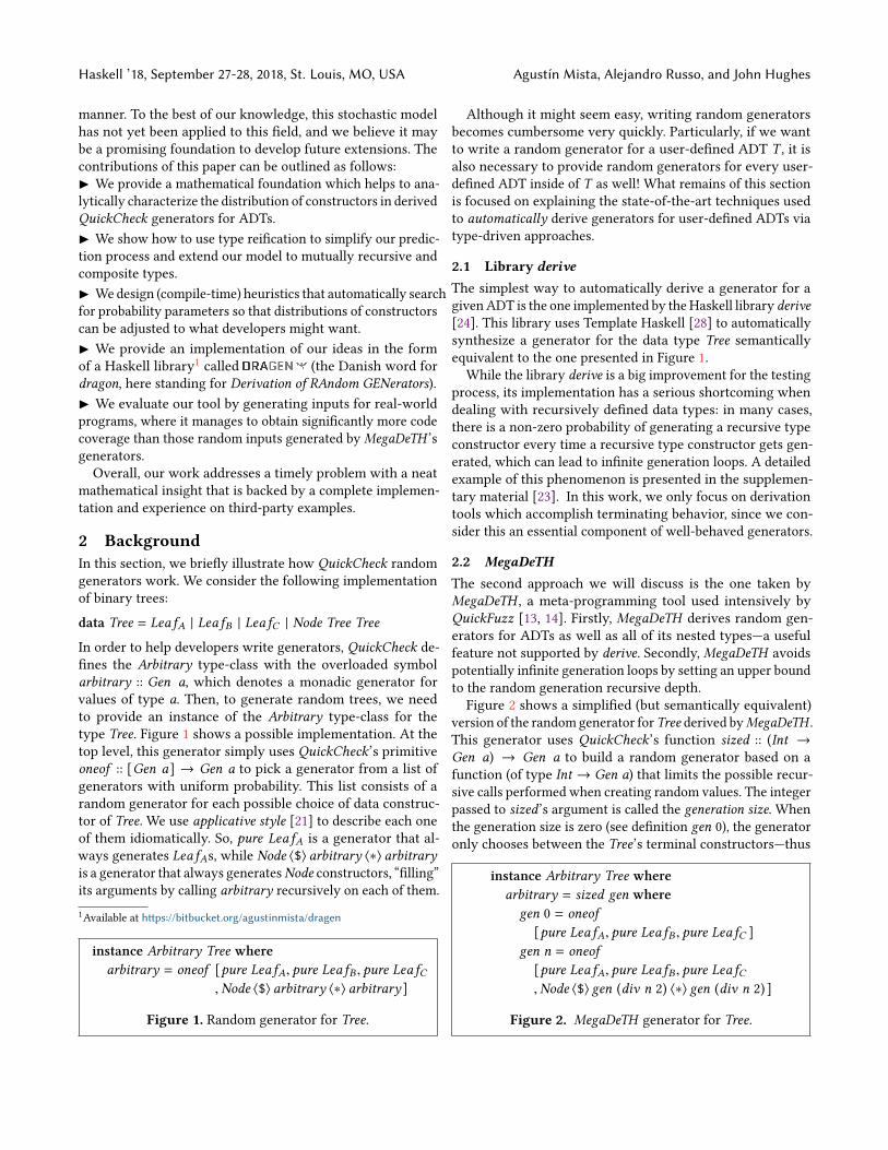
In order to help developers write generators, QuickCheck de-fines the Arbitrary type-class with the overloaded symbolarbitrary :: Gen a, which denotes a monadic generator forvalues of type a. Then, to generate random trees, we needto provide an instance of the Arbitrary type-class for thetype Tree. Figure 1 shows a possible implementation. At thetop level, this generator simply uses QuickCheck’s primitiveoneof :: [Gen a] → Gen a to pick a generator from a list ofgenerators with uniform probability. This list consists of arandom generator for each possible choice of data construc-tor of Tree. We use applicative style [21] to describe each oneof them idiomatically. So, pure LeafA is a generator that al-ways generates LeafAs, while Node ⟨$⟩ arbitrary ⟨∗⟩ arbitraryis a generator that always generatesNode constructors, “filling”its arguments by calling arbitrary recursively on each of them.1Available at https://bitbucket.org/agustinmista/dragen

instance Arbitrary Tree wherearbitrary = oneof [pure LeafA, pure LeafB , pure LeafC

,Node ⟨$⟩ arbitrary ⟨∗⟩ arbitrary ]

Figure 1. Random generator for Tree.

Although it might seem easy, writing random generatorsbecomes cumbersome very quickly. Particularly, if we wantto write a random generator for a user-defined ADT T , it isalso necessary to provide random generators for every user-defined ADT inside of T as well! What remains of this sectionis focused on explaining the state-of-the-art techniques usedto automatically derive generators for user-defined ADTs viatype-driven approaches.

2.1 Library deriveThe simplest way to automatically derive a generator for agivenADT is the one implemented by theHaskell library derive[24]. This library uses Template Haskell [28] to automaticallysynthesize a generator for the data type Tree semanticallyequivalent to the one presented in Figure 1.

While the library derive is a big improvement for the testingprocess, its implementation has a serious shortcoming whendealing with recursively defined data types: in many cases,there is a non-zero probability of generating a recursive typeconstructor every time a recursive type constructor gets gen-erated, which can lead to infinite generation loops. A detailedexample of this phenomenon is presented in the supplemen-tary material [23]. In this work, we only focus on derivationtools which accomplish terminating behavior, since we con-sider this an essential component of well-behaved generators.

2.2 MegaDeTHThe second approach we will discuss is the one taken byMegaDeTH , a meta-programming tool used intensively byQuickFuzz [13, 14]. Firstly, MegaDeTH derives random gen-erators for ADTs as well as all of its nested types—a usefulfeature not supported by derive. Secondly, MegaDeTH avoidspotentially infinite generation loops by setting an upper boundto the random generation recursive depth.Figure 2 shows a simplified (but semantically equivalent)

version of the randomgenerator for Tree derived byMegaDeTH .This generator uses QuickCheck’s function sized :: (Int →Gen a) → Gen a to build a random generator based on afunction (of type Int → Gen a) that limits the possible recur-sive calls performed when creating random values. The integerpassed to sized’s argument is called the generation size. Whenthe generation size is zero (see definition gen 0), the generatoronly chooses between the Tree’s terminal constructors—thus

instance Arbitrary Tree wherearbitrary = sized gen where

gen 0 = oneof[pure LeafA, pure LeafB , pure LeafC ]

gen n = oneof[pure LeafA, pure LeafB , pure LeafC,Node ⟨$⟩ gen (div n 2) ⟨∗⟩ gen (div n 2) ]

Figure 2. MegaDeTH generator for Tree.

https://bitbucket.org/agustinmista/dragen

Branching Processes for QuickCheck Generators Haskell ’18, September 27-28, 2018, St. Louis, MO, USA

ending the generation process. If the generation size is strictlypositive, it is free to randomly generate any Tree constructor(see definition gen n). When it chooses to generate a recursiveconstructor, it reduces the generation size for its subsequentrecursive calls by a factor that depends on the number of re-cursive arguments this constructor has (div n 2). In this way,MegaDeTH ensures that all generated values are finite.Although MegaDeTH generators always terminate, they

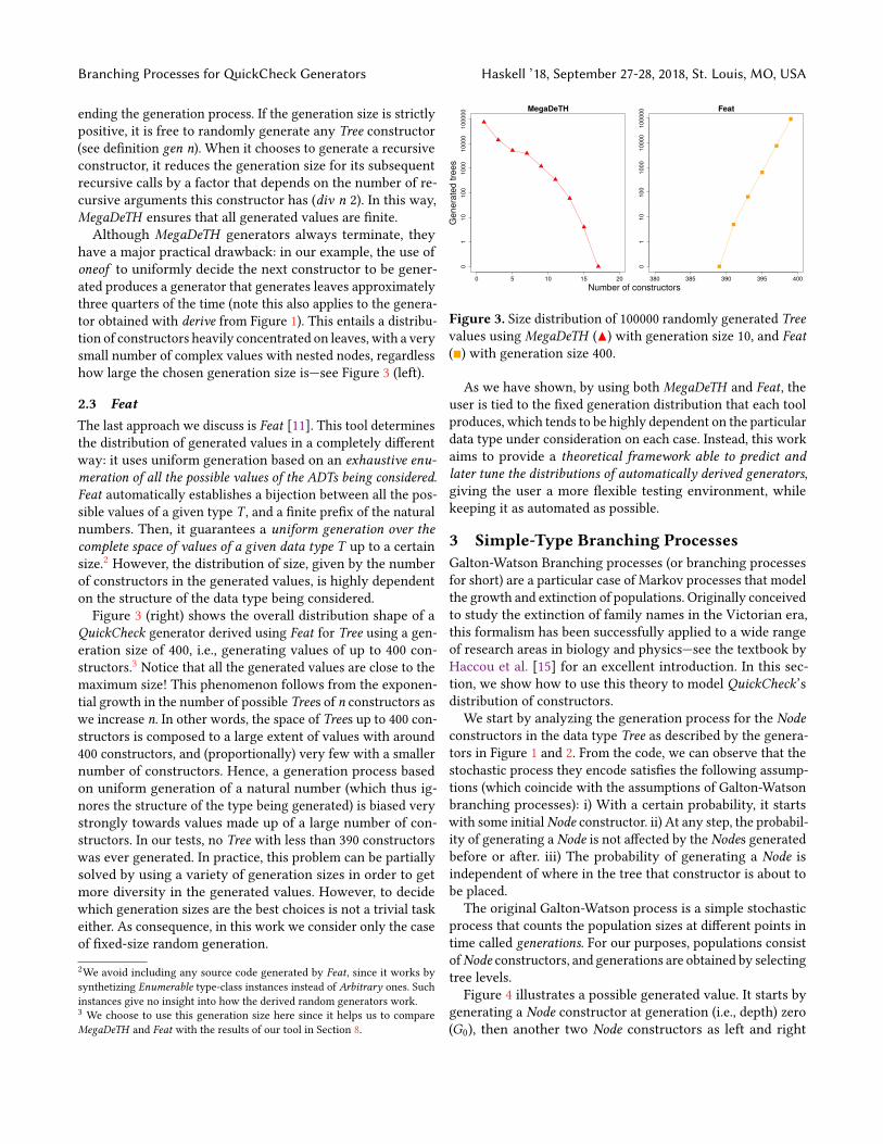
have a major practical drawback: in our example, the use ofoneof to uniformly decide the next constructor to be gener-ated produces a generator that generates leaves approximatelythree quarters of the time (note this also applies to the genera-tor obtained with derive from Figure 1). This entails a distribu-tion of constructors heavily concentrated on leaves, with a verysmall number of complex values with nested nodes, regardlesshow large the chosen generation size is—see Figure 3 (left).

2.3 FeatThe last approach we discuss is Feat [11]. This tool determinesthe distribution of generated values in a completely differentway: it uses uniform generation based on an exhaustive enu-meration of all the possible values of the ADTs being considered.Feat automatically establishes a bijection between all the pos-sible values of a given type T , and a finite prefix of the naturalnumbers. Then, it guarantees a uniform generation over thecomplete space of values of a given data type T up to a certainsize.2 However, the distribution of size, given by the numberof constructors in the generated values, is highly dependenton the structure of the data type being considered.Figure 3 (right) shows the overall distribution shape of a

QuickCheck generator derived using Feat for Tree using a gen-eration size of 400, i.e., generating values of up to 400 con-structors.3 Notice that all the generated values are close to themaximum size! This phenomenon follows from the exponen-tial growth in the number of possible Trees of n constructors aswe increase n. In other words, the space of Trees up to 400 con-structors is composed to a large extent of values with around400 constructors, and (proportionally) very few with a smallernumber of constructors. Hence, a generation process basedon uniform generation of a natural number (which thus ig-nores the structure of the type being generated) is biased verystrongly towards values made up of a large number of con-structors. In our tests, no Tree with less than 390 constructorswas ever generated. In practice, this problem can be partiallysolved by using a variety of generation sizes in order to getmore diversity in the generated values. However, to decidewhich generation sizes are the best choices is not a trivial taskeither. As consequence, in this work we consider only the caseof fixed-size random generation.

2We avoid including any source code generated by Feat, since it works bysynthetizing Enumerable type-class instances instead of Arbitrary ones. Suchinstances give no insight into how the derived random generators work.3 We choose to use this generation size here since it helps us to compareMegaDeTH and Feat with the results of our tool in Section 8.

Figure 3. Size distribution of 100000 randomly generated Treevalues using MegaDeTH (▲) with generation size 10, and Feat(■) with generation size 400.

As we have shown, by using both MegaDeTH and Feat, theuser is tied to the fixed generation distribution that each toolproduces, which tends to be highly dependent on the particulardata type under consideration on each case. Instead, this workaims to provide a theoretical framework able to predict andlater tune the distributions of automatically derived generators,giving the user a more flexible testing environment, whilekeeping it as automated as possible.

3 Simple-Type Branching ProcessesGalton-Watson Branching processes (or branching processesfor short) are a particular case of Markov processes that modelthe growth and extinction of populations. Originally conceivedto study the extinction of family names in the Victorian era,this formalism has been successfully applied to a wide rangeof research areas in biology and physics—see the textbook byHaccou et al. [15] for an excellent introduction. In this sec-tion, we show how to use this theory to model QuickCheck’sdistribution of constructors.We start by analyzing the generation process for the Node

constructors in the data type Tree as described by the genera-tors in Figure 1 and 2. From the code, we can observe that thestochastic process they encode satisfies the following assump-tions (which coincide with the assumptions of Galton-Watsonbranching processes): i) With a certain probability, it startswith some initialNode constructor. ii) At any step, the probabil-ity of generating a Node is not affected by the Nodes generatedbefore or after. iii) The probability of generating a Node isindependent of where in the tree that constructor is about tobe placed.The original Galton-Watson process is a simple stochastic

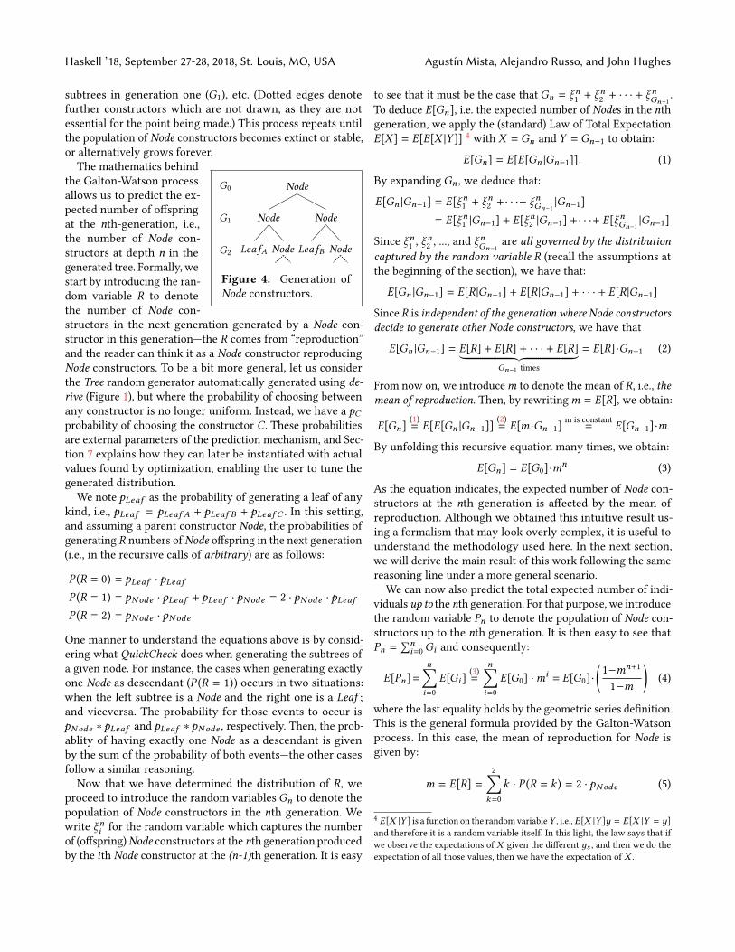
process that counts the population sizes at different points intime called generations. For our purposes, populations consistofNode constructors, and generations are obtained by selectingtree levels.Figure 4 illustrates a possible generated value. It starts by

generating a Node constructor at generation (i.e., depth) zero(G0), then another two Node constructors as left and right


subtrees in generation one (G1), etc. (Dotted edges denotefurther constructors which are not drawn, as they are notessential for the point being made.) This process repeats untilthe population of Node constructors becomes extinct or stable,or alternatively grows forever.

Node

Node

NodeLeafB

Node

NodeLeafA

G0

G1

G2

Figure 4. Generation ofNode constructors.

The mathematics behindthe Galton-Watson processallows us to predict the ex-pected number of offspringat the nth-generation, i.e.,the number of Node con-structors at depth n in thegenerated tree. Formally, westart by introducing the ran-dom variable R to denotethe number of Node con-structors in the next generation generated by a Node con-structor in this generation—the R comes from “reproduction”and the reader can think it as a Node constructor reproducingNode constructors. To be a bit more general, let us considerthe Tree random generator automatically generated using de-rive (Figure 1), but where the probability of choosing betweenany constructor is no longer uniform. Instead, we have a pCprobability of choosing the constructor C. These probabilitiesare external parameters of the prediction mechanism, and Sec-tion 7 explains how they can later be instantiated with actualvalues found by optimization, enabling the user to tune thegenerated distribution.

We note pLeaf as the probability of generating a leaf of anykind, i.e., pLeaf = pLeaf A + pLeaf B + pLeaf C . In this setting,and assuming a parent constructor Node, the probabilities ofgenerating R numbers of Node offspring in the next generation(i.e., in the recursive calls of arbitrary) are as follows:

P (R = 0) = pLeaf · pLeafP (R = 1) = pNode · pLeaf + pLeaf · pNode = 2 · pNode · pLeaf

P (R = 2) = pNode · pNode

One manner to understand the equations above is by consid-ering what QuickCheck does when generating the subtrees ofa given node. For instance, the cases when generating exactlyone Node as descendant (P (R = 1)) occurs in two situations:when the left subtree is a Node and the right one is a Leaf ;and viceversa. The probability for those events to occur ispNode ∗ pLeaf and pLeaf ∗ pNode , respectively. Then, the prob-ablity of having exactly one Node as a descendant is givenby the sum of the probability of both events—the other casesfollow a similar reasoning.Now that we have determined the distribution of R, we

proceed to introduce the random variables Gn to denote thepopulation of Node constructors in the nth generation. Wewrite ξni for the random variable which captures the numberof (offspring)Node constructors at the nth generation producedby the ith Node constructor at the (n-1)th generation. It is easy

to see that it must be the case thatGn = ξn1 + ξn2 + · · · + ξ

nGn−1

.To deduce E[Gn], i.e. the expected number of Nodes in the nthgeneration, we apply the (standard) Law of Total ExpectationE[X ] = E[E[X |Y ]] 4 with X = Gn and Y = Gn−1 to obtain:

E[Gn] = E[E[Gn |Gn−1]]. (1)

By expanding Gn , we deduce that:

E[Gn |Gn−1] = E[ξn1 + ξn2 +· · ·+ ξ

nGn−1|Gn−1]

= E[ξn1 |Gn−1] + E[ξn2 |Gn−1] +· · ·+ E[ξnGn−1|Gn−1]

Since ξn1 , ξn2 , ..., and ξ

nGn−1

are all governed by the distributioncaptured by the random variable R (recall the assumptions atthe beginning of the section), we have that:

E[Gn |Gn−1] = E[R |Gn−1] + E[R |Gn−1] + · · · + E[R |Gn−1]

SinceR is independent of the generation whereNode constructorsdecide to generate other Node constructors, we have that

E[Gn |Gn−1] = E[R] + E[R] + · · · + E[R]︸︷︷︸Gn−1 times

= E[R]·Gn−1 (2)

From now on, we introducem to denote the mean of R, i.e., themean of reproduction. Then, by rewritingm = E[R], we obtain:

E[Gn](1)= E[E[Gn |Gn−1]]

(2)= E[m ·Gn−1]

m is constant= E[Gn−1]·m

By unfolding this recursive equation many times, we obtain:

E[Gn] = E[G0]·mn (3)

As the equation indicates, the expected number of Node con-structors at the nth generation is affected by the mean ofreproduction. Although we obtained this intuitive result us-ing a formalism that may look overly complex, it is useful tounderstand the methodology used here. In the next section,we will derive the main result of this work following the samereasoning line under a more general scenario.

We can now also predict the total expected number of indi-viduals up to the nth generation. For that purpose, we introducethe random variable Pn to denote the population of Node con-structors up to the nth generation. It is then easy to see thatPn =

∑ni=0Gi and consequently:

E[Pn]=n∑i=0

E[Gi ](3)=

n∑i=0

E[G0] ·mi = E[G0]·(1−mn+1

1−m

)(4)

where the last equality holds by the geometric series definition.This is the general formula provided by the Galton-Watsonprocess. In this case, the mean of reproduction for Node isgiven by:

m = E[R] =2∑

k=0k · P (R = k ) = 2 · pNode (5)

4 E[X |Y ] is a function on the random variableY , i.e., E[X |Y ]y = E[X |Y = y]and therefore it is a random variable itself. In this light, the law says that ifwe observe the expectations of X given the different ys , and then we do theexpectation of all those values, then we have the expectation of X .


By (4) and (5), the expected number of Node constructors upto generation n is given by the following formula:

E[Pn]=E[G0]·(1−mn+1

1−m

)=pNode ·

(1− (2 · pNode )n+1

1−2·pNode

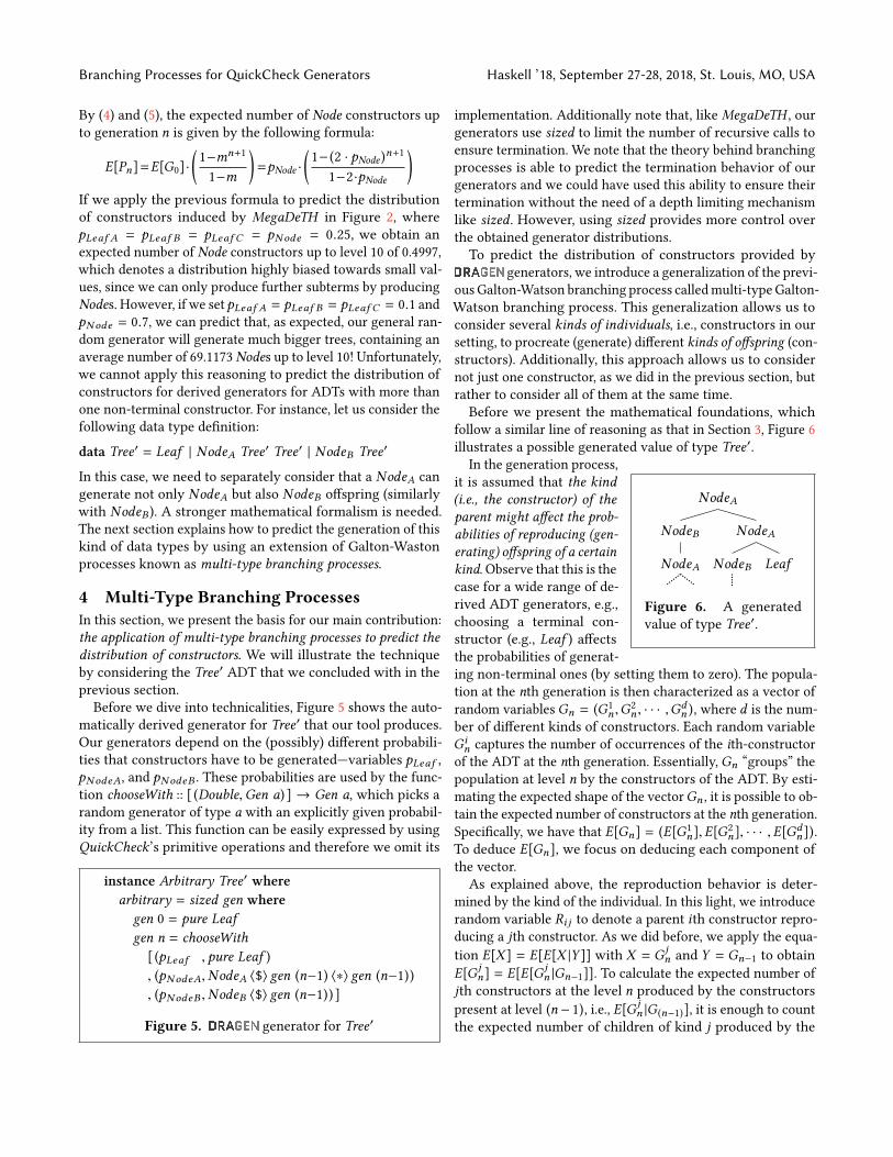
)If we apply the previous formula to predict the distributionof constructors induced by MegaDeTH in Figure 2, wherepLeaf A = pLeaf B = pLeaf C = pNode = 0.25, we obtain anexpected number of Node constructors up to level 10 of 0.4997,which denotes a distribution highly biased towards small val-ues, since we can only produce further subterms by producingNodes. However, if we setpLeaf A = pLeaf B = pLeaf C = 0.1 andpNode = 0.7, we can predict that, as expected, our general ran-dom generator will generate much bigger trees, containing anaverage number of 69.1173 Nodes up to level 10! Unfortunately,we cannot apply this reasoning to predict the distribution ofconstructors for derived generators for ADTs with more thanone non-terminal constructor. For instance, let us consider thefollowing data type definition:

data Tree′ = Leaf | NodeA Tree′ Tree′ | NodeB Tree′

In this case, we need to separately consider that a NodeA cangenerate not only NodeA but also NodeB offspring (similarlywith NodeB ). A stronger mathematical formalism is needed.The next section explains how to predict the generation of thiskind of data types by using an extension of Galton-Wastonprocesses known as multi-type branching processes.

4 Multi-Type Branching ProcessesIn this section, we present the basis for our main contribution:the application of multi-type branching processes to predict thedistribution of constructors. We will illustrate the techniqueby considering the Tree′ ADT that we concluded with in theprevious section.

Before we dive into technicalities, Figure 5 shows the auto-matically derived generator for Tree′ that our tool produces.Our generators depend on the (possibly) different probabili-ties that constructors have to be generated—variables pLeaf ,pNodeA, and pNodeB . These probabilities are used by the func-tion chooseWith :: [ (Double,Gen a) ] → Gen a, which picks arandom generator of type a with an explicitly given probabil-ity from a list. This function can be easily expressed by usingQuickCheck’s primitive operations and therefore we omit its

instance Arbitrary Tree′ wherearbitrary = sized gen where

gen 0 = pure Leafgen n = chooseWith[ (pLeaf , pure Leaf ), (pNodeA,NodeA ⟨$⟩ gen (n−1) ⟨∗⟩ gen (n−1)), (pNodeB ,NodeB ⟨$⟩ gen (n−1)) ]

Figure 5. generator for Tree′

implementation. Additionally note that, like MegaDeTH , ourgenerators use sized to limit the number of recursive calls toensure termination. We note that the theory behind branchingprocesses is able to predict the termination behavior of ourgenerators and we could have used this ability to ensure theirtermination without the need of a depth limiting mechanismlike sized. However, using sized provides more control overthe obtained generator distributions.To predict the distribution of constructors provided by

generators, we introduce a generalization of the previ-ous Galton-Watson branching process calledmulti-typeGalton-Watson branching process. This generalization allows us toconsider several kinds of individuals, i.e., constructors in oursetting, to procreate (generate) different kinds of offspring (con-structors). Additionally, this approach allows us to considernot just one constructor, as we did in the previous section, butrather to consider all of them at the same time.Before we present the mathematical foundations, which

follow a similar line of reasoning as that in Section 3, Figure 6illustrates a possible generated value of type Tree′.

NodeA

NodeA

LeafNodeB

NodeB

NodeA

Figure 6. A generatedvalue of type Tree′.

In the generation process,it is assumed that the kind(i.e., the constructor) of theparent might affect the prob-abilities of reproducing (gen-erating) offspring of a certainkind. Observe that this is thecase for a wide range of de-rived ADT generators, e.g.,choosing a terminal con-structor (e.g., Leaf ) affectsthe probabilities of generat-ing non-terminal ones (by setting them to zero). The popula-tion at the nth generation is then characterized as a vector ofrandom variablesGn = (G1

n ,G2n , · · · ,G

dn ), where d is the num-

ber of different kinds of constructors. Each random variableGin captures the number of occurrences of the ith-constructor

of the ADT at the nth generation. Essentially,Gn “groups” thepopulation at level n by the constructors of the ADT. By esti-mating the expected shape of the vectorGn , it is possible to ob-tain the expected number of constructors at the nth generation.Specifically, we have that E[Gn] = (E[G1

n],E[G2n], · · · ,E[Gd

n ]).To deduce E[Gn], we focus on deducing each component ofthe vector.As explained above, the reproduction behavior is deter-

mined by the kind of the individual. In this light, we introducerandom variable Ri j to denote a parent ith constructor repro-ducing a jth constructor. As we did before, we apply the equa-tion E[X ] = E[E[X |Y ]] with X = G j

n and Y = Gn−1 to obtainE[G j

n] = E[E[G jn |Gn−1]]. To calculate the expected number of

jth constructors at the level n produced by the constructorspresent at level (n− 1), i.e., E[G j

n |G (n−1)], it is enough to countthe expected number of children of kind j produced by the


different parents of kind i , i.e., E[Ri j ], times the amount ofparents of kind i found in the level (n − 1), i.e., Gi

(n−1) . Thisresult is expressed by the following equation marked as (⋆),and is formally verified in the supplementary material.

E[G jn |Gn−1]

(⋆)=

d∑i=1

Gi(n−1) ·E[Ri j ] =

d∑i=1

Gi(n−1) ·mi j (6)

Similarly as before, we rewrite E[Ri j ] as mi j , which nowrepresents a single expectation of reproduction indexed by thekind of both the parent and child constructor.

Mean matrix of constructors In the previous section, mwas the expectation of reproduction of a single constructor.Now we havemi j as the expectation of reproduction indexedby the parent and child constructor. In this light, we defineMC , the mean matrix of constructors (or mean matrix for sim-plicity) such that eachmi j stores the expected number of jthconstructors generated by the ith constructor.MC is a param-eter of the Galton-Watson multi-type process and can be builtat compile-time using statically known type information. Weare now able to deduce E[G j

n].

E[G jn] = E[E[G j

n |Gn−1]](6)= E

d∑i=1

Gi(n−1) ·mi j

=

d∑i=1

E[Gi(n−1) ·mi j ] =

d∑i=1

E[Gi(n−1)]·mi j

Using this last equation, we can rewrite E[Gn] as follows.

E[Gn] = *,

d∑i=1

E[G1(n−1)]·mi1, · · · ,

d∑i=1

E[Gd(n−1)]·mid+

-By linear algebra, we can rewrite the vector above as thematrix multiplication E[Gn]T = E[Gn−1]T ·MC . By repeatedlyunfolding this definition, we obtain that:

E[Gn]T = E[G0]T · (MC )n (7)

This equation is a generalization of (3) when considering manyconstructors. As we did before, we introduce a random variablePn =

∑ni=0Gi to denote the population up to the nth generation.

It is now possible to obtain the expected population of all theconstructors but in a clustered manner:

E[Pn]T = E

n∑i=0

Gi

T

=

n∑i=0

E[Gi ]T(7)=

n∑i=0

E[G0]T · (MC )n (8)

It is possible to write the resulting sum as the closed formula:

E[Pn]T = E[G0]T ·(I − (MC )

n+1

I −MC

)(9)

where I represents the identity matrix of the appropriate size.Note that equation (9) only holds when (I − MC ) is non-singular, however, this is the usual case. When (I − MC ) issingular, we resort to using equation (8) instead. Without los-ing generality, and for simplicity, we consider equations (8)

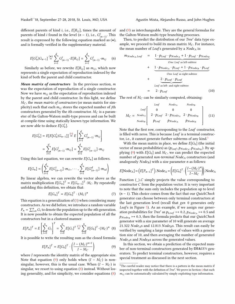
and (9) as interchangeable. They are the general formulas forthe Galton-Watson multi-type branching processes.Then, to predict the distribution of our Tree′ data type ex-

ample, we proceed to build its mean matrixMC . For instance,the mean number of Leaf s generated by a NodeA is:

mNodeA,Leaf = 1 · pLeaf · pNodeA + 1 · pLeaf · pNodeB︸︷︷︸One Leaf as left-subtree

+ 1 · pNodeA · pLeaf + 1 · pNodeB · pLeaf︸︷︷︸One Leaf as right-subtree

+ 2 · pLeaf · pLeaf︸︷︷︸Leaf as left- and right-subtree

= 2 · pLeaf (10)

The rest ofMC can be similarly computed, obtaining:

MC =

0 0 02 · pLeaf 2 · pNodeA 2 · pNodeB

pLeaf pNodeA pNodeB

Leaf NodeA NodeB

Leaf

NodeA

NodeB

(11)

Note that the first row, corresponding to the Leaf constructor,is filled with zeros. This is because Leaf is a terminal construc-tor, i.e., it cannot generate further subterms of any kind.5

With the mean matrix in place, we define E[G0] (the initialvector of mean probabilities) as (pLeaf ,pNodeA ,pNodeB ). By ap-plying (9) with E[G0] and MC , we can predict the expectednumber of generated non-terminal NodeA constructors (andanalogously NodeB ) with a size parameter n as follows:

E[NodeA]=(E[Pn−1]T

).NodeA=

(E[G0]T ·

(I− (MC )

n

I−MC

)).NodeA

Function (_).C simply projects the value corresponding toconstructor C from the population vector. It is very importantto note that the sum only includes the population up to level(n − 1). This choice comes from the fact that our QuickCheckgenerator can choose between only terminal constructors atthe last generation level (recall that gen 0 generates onlyLeaf s in Figure 5). As an example, if we assign our gener-ation probabilities for Tree′ as pLeaf 7→ 0.2, pNodeA 7→ 0.5 andpNodeB 7→ 0.3, then the formula predicts that our QuickCheckgenerator with a size parameter of 10 will generate on average21.322 NodeAs and 12.813 NodeBs. This result can easily beverified by sampling a large number of values with a genera-tion size of 10, and then averaging the number of generatedNodeAs and NodeBs across the generated values.

In this section, we obtain a prediction of the expected num-ber of non-terminal constructors generated by gen-erators. To predict terminal constructors, however, requires aspecial treatment as discussed in the next section.

5The careful reader may notice that there is a pattern in the mean matrix ifinspected together with the definition of Tree′. We prove in Section 6 that eachmi j can be automatically calculated by simply exploiting type information.


5 Terminal constructorsIn this section we introduce the special treatment required topredict the generated distribution of terminal constructors, i.e.constructors with no recursive arguments.Consider the generator in Figure 5. It generates terminal

constructors in two situations, i.e., in the definition of gen 0and gen n. In other words, the random process introduced byour generators can be considered to be composed of two inde-pendent parts when it comes to terminal constructors—referto the supplementary material for a graphical interpretation.In principle, the number of terminal constructors generatedby the stochastic process described in gen n is captured bythe multi-type branching process formulas. However, to pre-dict the expected number of terminal constructors generatedby exercising gen 0, we need to separately consider a randomprocess that only generates terminal constructors in order to ter-minate. For this purpose, and assuming a maximum generationdepth n, we need to calculate the number of terminal construc-tors required to stop the generation process at the recursive ar-guments of each non-terminal constructor at level (n−1). In ourTree′ example, this corresponds to two Leaf s for every NodeAand one Leaf for every NodeB constructor at level (n − 1).Since both random processes are independent, to predict

the overall expected number of terminal constructors, we cansimply add the expected number of terminal constructors gen-erated in each one of them. Recalling our previous example,we obtain the following formula for Tree′ terminals as follows:

E[Leaf ] =(E[Pn−1]T

).Leaf︸︷︷︸

branching process

+ 2·(E[Gn−1]T

).NodeA︸︷︷︸

case (NodeA Leaf Leaf )

+ 1·(E[Gn−1]T

).NodeB︸︷︷︸

case (NodeB Leaf )

The formula counts the Leaf s generated by the multi-typebranching process up to level (n − 1) and adds the expectednumber of Leaf s generated at the last level.

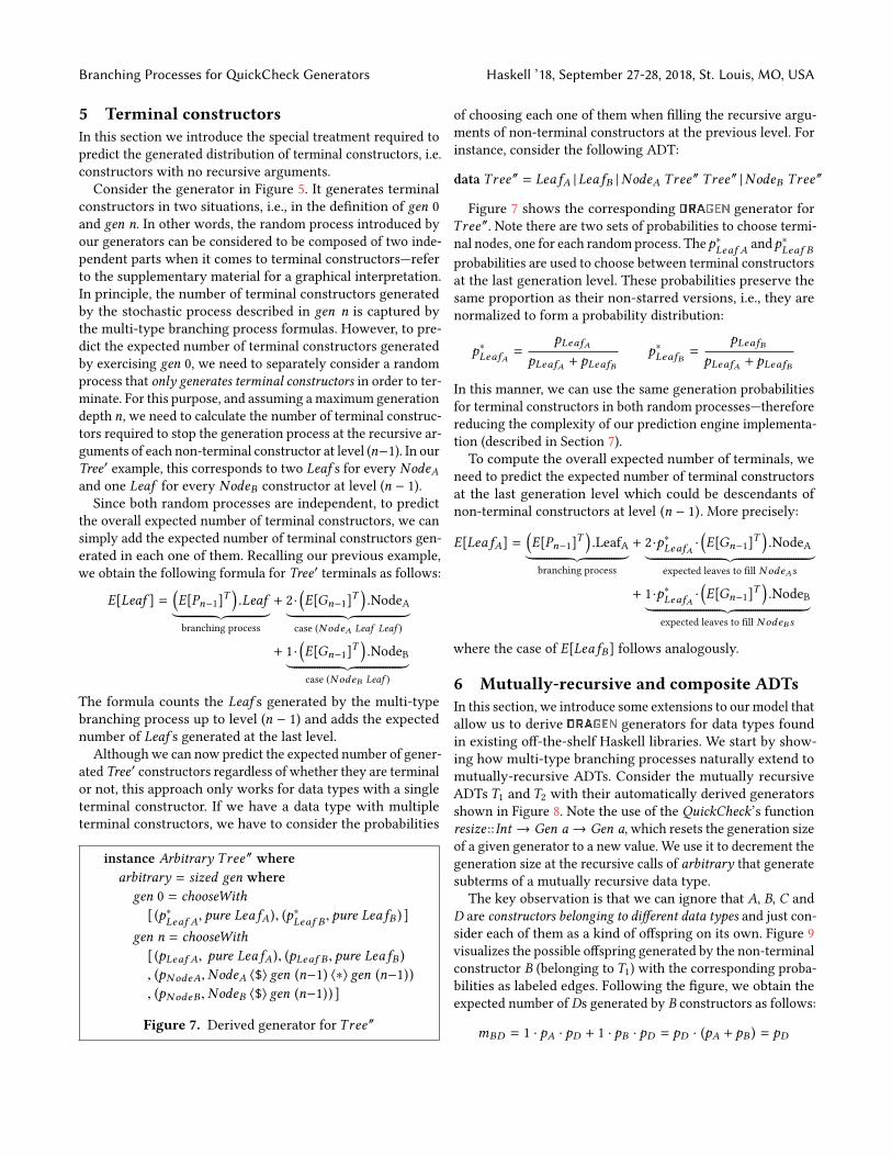
Although we can now predict the expected number of gener-ated Tree′ constructors regardless of whether they are terminalor not, this approach only works for data types with a singleterminal constructor. If we have a data type with multipleterminal constructors, we have to consider the probabilities

instance Arbitrary Tree ′′ wherearbitrary = sized gen where

gen 0 = chooseWith[ (p∗Leaf A, pure LeafA), (p

∗Leaf B , pure LeafB ) ]

gen n = chooseWith[ (pLeaf A, pure LeafA), (pLeaf B , pure LeafB ), (pNodeA,NodeA ⟨$⟩ gen (n−1) ⟨∗⟩ gen (n−1)), (pNodeB ,NodeB ⟨$⟩ gen (n−1)) ]

Figure 7. Derived generator for Tree ′′

of choosing each one of them when filling the recursive argu-ments of non-terminal constructors at the previous level. Forinstance, consider the following ADT:

data Tree ′′ = LeafA |LeafB |NodeA Tree ′′ Tree ′′ |NodeB Tree ′′

Figure 7 shows the corresponding generator forTree ′′. Note there are two sets of probabilities to choose termi-nal nodes, one for each random process. Thep∗Leaf A andp∗Leaf Bprobabilities are used to choose between terminal constructorsat the last generation level. These probabilities preserve thesame proportion as their non-starred versions, i.e., they arenormalized to form a probability distribution:

p∗LeafA =pLeafA

pLeafA + pLeafBp∗LeafB =

pLeafBpLeafA + pLeafB

In this manner, we can use the same generation probabilitiesfor terminal constructors in both random processes—thereforereducing the complexity of our prediction engine implementa-tion (described in Section 7).To compute the overall expected number of terminals, we

need to predict the expected number of terminal constructorsat the last generation level which could be descendants ofnon-terminal constructors at level (n − 1). More precisely:

E[LeafA] =(E[Pn−1]T

).LeafA︸︷︷︸

branching process

+ 2·p∗LeafA ·(E[Gn−1]T

).NodeA︸︷︷︸

expected leaves to fill NodeAs

+ 1·p∗LeafA ·(E[Gn−1]T

).NodeB︸︷︷︸

expected leaves to fill NodeBs

where the case of E[LeafB] follows analogously.

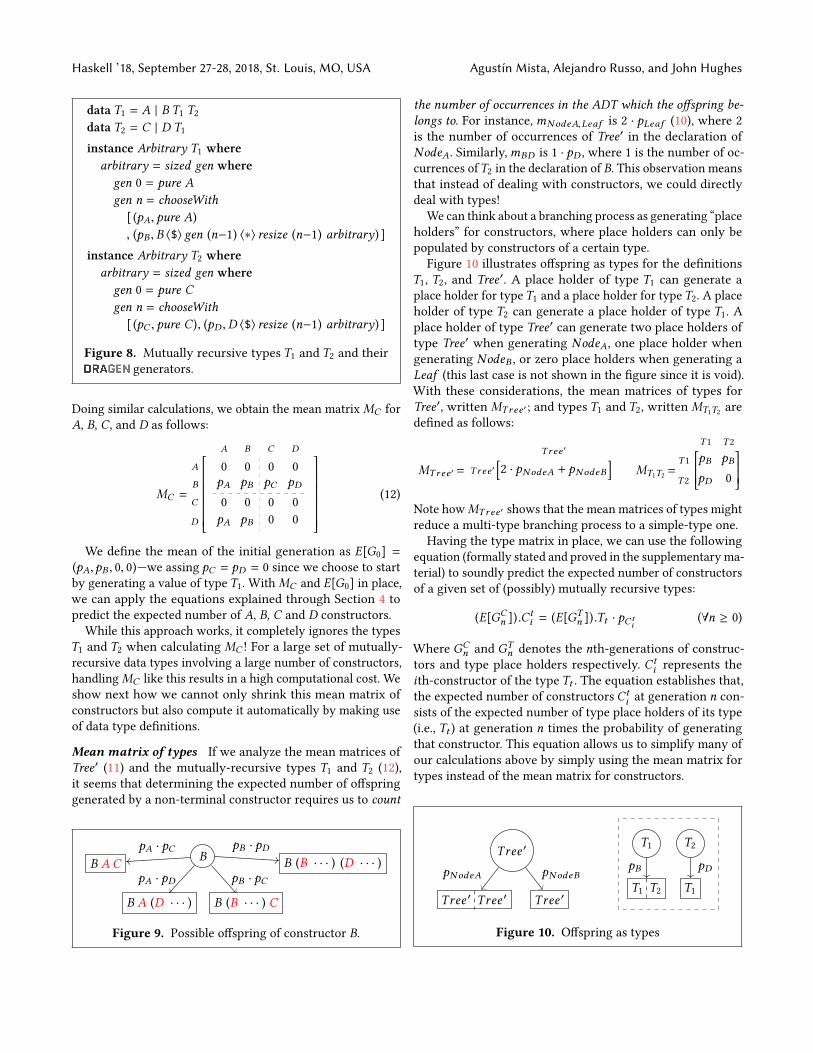
6 Mutually-recursive and composite ADTsIn this section, we introduce some extensions to our model thatallow us to derive generators for data types foundin existing off-the-shelf Haskell libraries. We start by show-ing how multi-type branching processes naturally extend tomutually-recursive ADTs. Consider the mutually recursiveADTs T1 and T2 with their automatically derived generatorsshown in Figure 8. Note the use of the QuickCheck’s functionresize ::Int → Gen a→ Gen a, which resets the generation sizeof a given generator to a new value. We use it to decrement thegeneration size at the recursive calls of arbitrary that generatesubterms of a mutually recursive data type.

The key observation is that we can ignore that A, B, C andD are constructors belonging to different data types and just con-sider each of them as a kind of offspring on its own. Figure 9visualizes the possible offspring generated by the non-terminalconstructor B (belonging to T1) with the corresponding proba-bilities as labeled edges. Following the figure, we obtain theexpected number of Ds generated by B constructors as follows:

mBD = 1 · pA · pD + 1 · pB · pD = pD · (pA + pB ) = pD


data T1 = A | B T1 T2data T2 = C | D T1

instance Arbitrary T1 wherearbitrary = sized gen wheregen 0 = pure Agen n = chooseWith[ (pA, pure A), (pB ,B ⟨$⟩ gen (n−1) ⟨∗⟩ resize (n−1) arbitrary) ]

instance Arbitrary T2 wherearbitrary = sized gen wheregen 0 = pure Cgen n = chooseWith[ (pC , pure C), (pD ,D ⟨$⟩ resize (n−1) arbitrary) ]

Figure 8. Mutually recursive types T1 and T2 and theirgenerators.

Doing similar calculations, we obtain the mean matrixMC forA, B, C, and D as follows:

MC =

0 0 0 0pA pB pC pD

0 0 0 0pA pB 0 0

A B C D

A

B

C

D

(12)

We define the mean of the initial generation as E[G0] =(pA,pB , 0, 0)—we assing pC = pD = 0 since we choose to startby generating a value of type T1. WithMC and E[G0] in place,we can apply the equations explained through Section 4 topredict the expected number of A, B, C and D constructors.

While this approach works, it completely ignores the typesT1 and T2 when calculating MC ! For a large set of mutually-recursive data types involving a large number of constructors,handlingMC like this results in a high computational cost. Weshow next how we cannot only shrink this mean matrix ofconstructors but also compute it automatically by making useof data type definitions.

Mean matrix of types If we analyze the mean matrices ofTree′ (11) and the mutually-recursive types T1 and T2 (12),it seems that determining the expected number of offspringgenerated by a non-terminal constructor requires us to count

BB A C

pA · pC

B A (D · · · )

pA · pD

B (B · · · ) C

pB · pC

B (B · · · ) (D · · · )

pB · pD

Figure 9. Possible offspring of constructor B.

the number of occurrences in the ADT which the offspring be-longs to. For instance,mNodeA,Leaf is 2 · pLeaf (10), where 2is the number of occurrences of Tree′ in the declaration ofNodeA. Similarly,mBD is 1 · pD , where 1 is the number of oc-currences ofT2 in the declaration of B. This observation meansthat instead of dealing with constructors, we could directlydeal with types!

We can think about a branching process as generating “placeholders” for constructors, where place holders can only bepopulated by constructors of a certain type.Figure 10 illustrates offspring as types for the definitions

T1, T2, and Tree′. A place holder of type T1 can generate aplace holder for typeT1 and a place holder for typeT2. A placeholder of type T2 can generate a place holder of type T1. Aplace holder of type Tree′ can generate two place holders oftype Tree′ when generating NodeA, one place holder whengenerating NodeB , or zero place holders when generating aLeaf (this last case is not shown in the figure since it is void).With these considerations, the mean matrices of types forTree′, written MT ree ′ ; and types T1 and T2, written MT1T2 aredefined as follows:

MT ree ′ = 2 · pNodeA + pNodeB[ ]T ree ′

T ree ′ MT1T2 =pB pB

pD 0

T 1 T 2

T 1

T 2

Note howMT ree ′ shows that the mean matrices of types mightreduce a multi-type branching process to a simple-type one.Having the type matrix in place, we can use the following

equation (formally stated and proved in the supplementary ma-terial) to soundly predict the expected number of constructorsof a given set of (possibly) mutually recursive types:

(E[GCn ]).C

ti = (E[GT

n ]).Tt · pC ti

(∀n ≥ 0)

Where GCn and GT

n denotes the nth-generations of construc-tors and type place holders respectively. Ct

i represents theith-constructor of the type Tt . The equation establishes that,the expected number of constructors Ct

i at generation n con-sists of the expected number of type place holders of its type(i.e., Tt ) at generation n times the probability of generatingthat constructor. This equation allows us to simplify many ofour calculations above by simply using the mean matrix fortypes instead of the mean matrix for constructors.

Tree ′

Tree ′ Tree ′

pNodeA

Tree ′

pNodeB

T1

T1 T2

pB

T2

T1

pD

Figure 10. Offspring as types


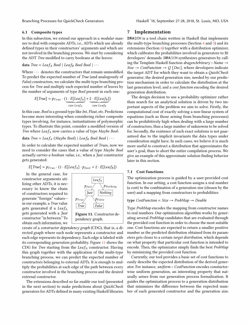
6.1 Composite typesIn this subsection, we extend our approach in a modular man-ner to deal with composite ADTs, i.e., ADTs which use alreadydefined types in their constructors’ arguments and which arenot involved in the branching process. We start by consideringthe ADT Tree modified to carry booleans at the leaves:

data Tree = LeafA Bool | LeafB Bool Bool | · · ·

Where · · · denotes the constructors that remain unmodified.To predict the expected number of True (and analogously ofFalse) constructors, we calculate the multi-type branching pro-cess for Tree and multiply each expected number of leaves bythe number of arguments of type Bool present in each one:

E[True] = pT rue · (1 · E[LeafA]︸︷︷︸case LeafA

+ 2 · E[LeafB]︸︷︷︸case LeafB

)

In this case, Bool is a ground type like Int, Float, etc. Predictionsbecome more interesting when considering richer compositetypes involving, for instance, instantiations of polymorphictypes. To illustrate this point, consider a modified version ofTree where LeafA now carries a value of type Maybe Bool:

data Tree = LeafA (Maybe Bool) | LeafB Bool Bool | · · ·

In order to calculate the expected number of Trues, now weneed to consider the cases that a value of type Maybe Boolactually carries a boolean value, i.e., when a Just constructorgets generated:

E[True] = pT rue · (1 · E[LeafA] · p Just + 2 · E[LeafB])

LeafA

Just

True

pT rue

False

pFalse

p Just

Nothing

pNothinд

Figure 11. Constructor de-pendency graph.

In the general case, forconstructor arguments uti-lizing other ADTs, it is nec-essary to know the chainof constructors required togenerate “foreign” values—in our example, a True valuegets generated if a LeafAgets generated with a Justconstructor “in between.” Toobtain such information, wecreate of a constructor dependency graph (CDG), that is, a di-rected graph where each node represents a constructor andeach edge represents its dependency. Each edge is labeled withits corresponding generation probability. Figure 11 shows theCDG for Tree starting from the LeafA constructor. Havingthis graph together with the application of the multi-typebranching process, we can predict the expected number ofconstructors belonging to external ADTs. It is enough to mul-tiply the probabilities at each edge of the path between everyconstructor involved in the branching process and the desiredexternal constructor.The extensions described so far enable our tool (presented

in the next section) to make predictions about QuickCheckgenerators for ADTs defined in many existing Haskell libraries.

7 Implementationis a tool chain written in Haskell that implements

the multi-type branching processes (Section 4 and 5) and itsextensions (Section 6) together with a distribution optimizer,which calibrates the probabilities involved in generators to fitdevelopers’ demands. synthesizes generators by call-ing the Template Haskell function dragenArbitrary ::Name →Size → CostFunction → Q [Dec ], where developers indicatethe target ADT for which they want to obtain a QuickCheckgenerator; the desired generation size, needed by our predic-tion mechanism in order to calculate the distribution at thelast generation level; and a cost function encoding the desiredgeneration distribution.The design decision to use a probability optimizer rather

than search for an analytical solution is driven by two im-portant aspects of the problem we aim to solve. Firstly, thecomputational cost of exactly solving a non-linear system ofequations (such as those arising from branching processes)can be prohibitively high when dealing with a large numberof constructors, thus a large number of unknowns to be solvedfor. Secondly, the existence of such exact solutions is not guar-anteed due to the implicit invariants the data types underconsideration might have. In such cases, we believe it is muchmore useful to construct a distribution that approximates theuser’s goal, than to abort the entire compilation process. Wegive an example of this approximate solution finding behaviorlater in this section.

7.1 Cost functionsThe optimization process is guided by a user-provided costfunction. In our setting, a cost function assigns a real number(a cost) to the combination of a generation size (chosen by theuser) and a mapping from constructors to probabilities:

type CostFunction = Size → ProbMap → Double

Type ProbMap encodes the mapping from constructor namesto real numbers. Our optimization algorithm works by gener-ating several ProbMap candidates that are evaluated throughthe provided cost function in order to choose the most suitableone. Cost functions are expected to return a smaller positivenumber as the predicted distribution obtained from its param-eters gets closer to a certain target distribution, which dependson what property that particular cost function is intended toencode. Then, the optimizator simply finds the best ProbMapby minimizing the provided cost function.

Currently, our tool provides a basic set of cost functions toeasily describe the expected distribution of the derived gener-ator. For instance, uniform :: CostFunction encodes constuctor-wise uniform generation, an interesting property that nat-urally arises from our generation process formalization. Itguides the optimization process to a generation distributionthat minimizes the difference between the expected num-ber of each generated constructor and the generation size.


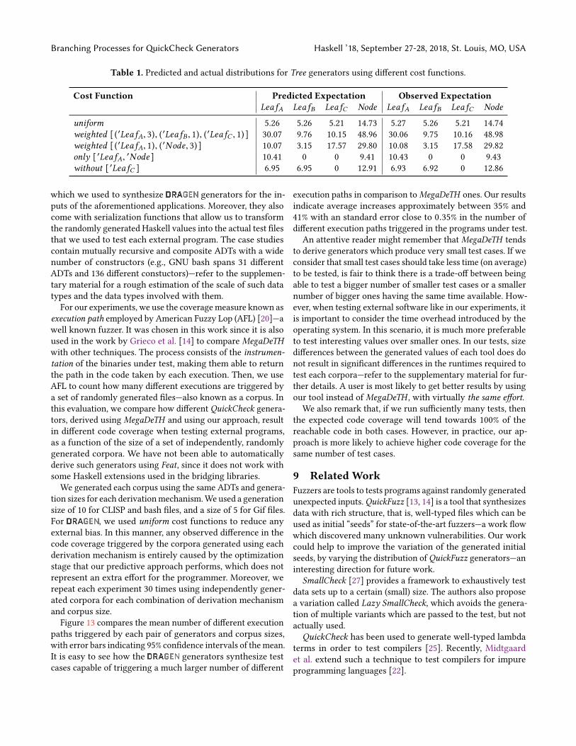
Moreover, the user can restrict the generation distributionto a certain subset of constructors using the cost functionsonly :: [Name] → CostFunction and without :: [Name] →CostFunction to describe these restrictions. In this case, thewhitelisted constructors are then generated following theuniform behavior. Similarly, if the branching process involvesmutually recursive data types, the user could restrict the gen-eration to a certain subset of data types by using the func-tions onlyTypes and withoutTypes. Additionally, when the userwants to generate constructors according to certain propor-tions, weighted :: [ (Name, Int) ]→ CostFunction allows to en-code this property, e.g. three times more LeafA’s than LeafB ’s.Table 1 shows the number of expected and observed con-

structors of different Tree generators obtained by using differ-ent cost functions. The observed expectations were calculatedaveraging the number of constructors across 100000 gener-ated values. Firstly, note how the generated distributions aresoundly predicted by our tool. In our tests, the small differencesbetween predictions and actual values dissapear as we increasethe number of generated values. As for the cost functions’ be-havior, there are some interesting aspects to note. For instance,in the uniform case the optimizer cannot do anything to breakthe implicit invariant of the data type: every binary tree with nnodes has n + 1 leaves. Instead, it converges to a solution that“approximates” a uniform distribution around the generationsize parameter. We believe this is desirable behavior, to findan approximate solution when certain invariants prevent theoptimization process from finding an exact solution. This waythe user does not have to be aware of the possible invariantsthat the target data type may have, obtaining a solution thatis good enough for most purposes. On the other hand, noticethat in the weighted case at the second row of Table 1, theexpected number of generated Nodes is considerably large.This constructor is not listed in the proportions list, hencethe optimizer can freely adjust its probability to satisfy theproportions specified for the leaves.

7.2 Derivation Process’s derivation process starts at compile-timewith a type

reification stage that extracts information about the structureof the types under consideration. It follows an intermediatestage composed of the optimizer for probabilities used in gen-erators, which is guided by our multi-type branching processmodel, parametrized on the cost function provided. This opti-mizer is based on a standard local-search optimization algo-rithm that recursively chooses the best mapping from construc-tors to probabilities in the current neighborhood. Neighborsare ProbMaps, determined by individually varying the prob-abilities for each constructor with a predetermined ∆. Then,to determine the “best” probabilities, the local-search appliesour prediction mechanishm to the immediate neighbors thathave not yet been visited by evaluating the cost function toselect the most suitable next candidate. This process contin-ues until a local minimum is reached when there are no new

neighbors to evaluate, or if each step improvement is lowerthan a minimum predetermined ε .The final stage synthesizes a Arbitrary type-class instance

for the target data types using the optimized generation prob-abilities. For this stage, we extend some functionality presentin MegaDeTH in order to derive generators parametrized byour previously optimized probabilities. Refer to the supple-mentary material for further details on the cost functions andalgorithms addressed by this section.

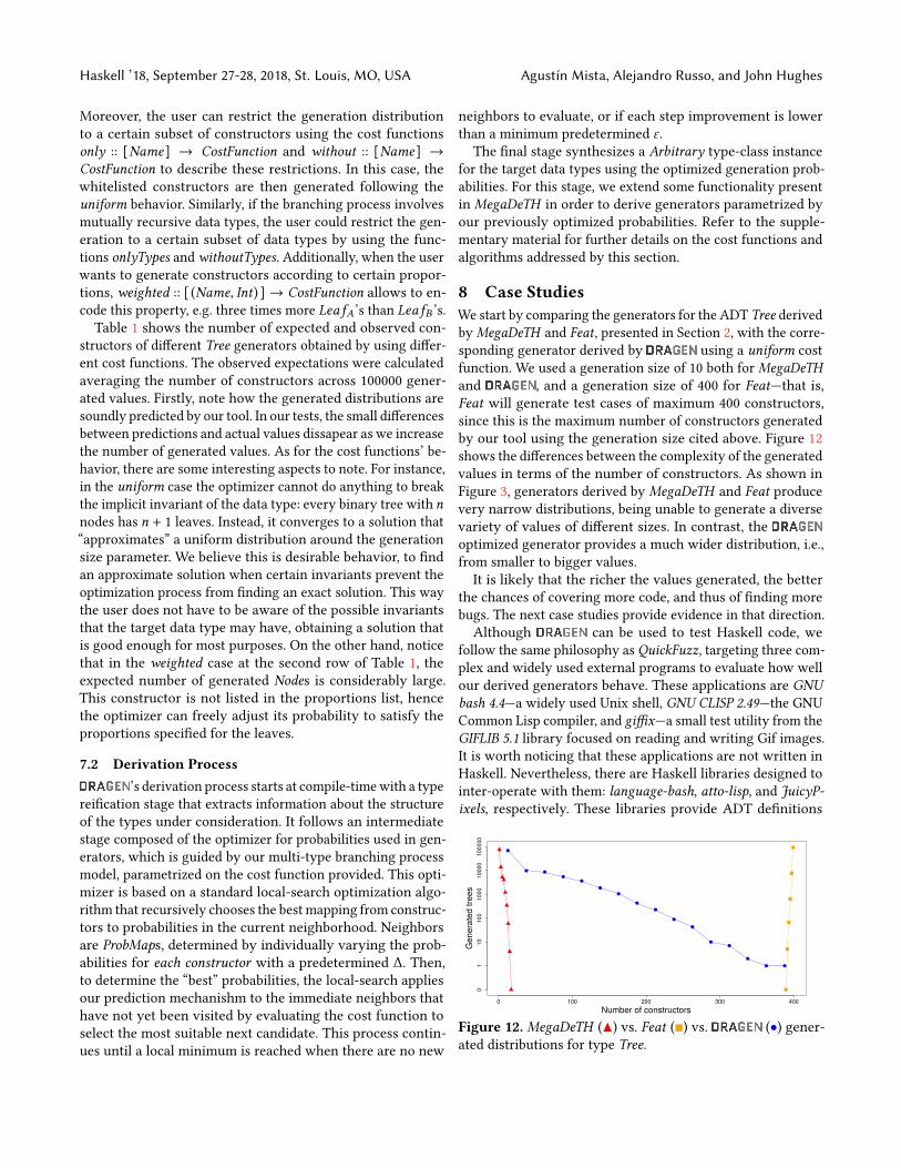
8 Case StudiesWe start by comparing the generators for the ADT Tree derivedby MegaDeTH and Feat, presented in Section 2, with the corre-sponding generator derived by using a uniform costfunction. We used a generation size of 10 both for MegaDeTHand , and a generation size of 400 for Feat—that is,Feat will generate test cases of maximum 400 constructors,since this is the maximum number of constructors generatedby our tool using the generation size cited above. Figure 12shows the differences between the complexity of the generatedvalues in terms of the number of constructors. As shown inFigure 3, generators derived by MegaDeTH and Feat producevery narrow distributions, being unable to generate a diversevariety of values of different sizes. In contrast, theoptimized generator provides a much wider distribution, i.e.,from smaller to bigger values.It is likely that the richer the values generated, the better

the chances of covering more code, and thus of finding morebugs. The next case studies provide evidence in that direction.Although can be used to test Haskell code, we

follow the same philosophy as QuickFuzz, targeting three com-plex and widely used external programs to evaluate how wellour derived generators behave. These applications are GNUbash 4.4—a widely used Unix shell, GNU CLISP 2.49—the GNUCommon Lisp compiler, and giffix—a small test utility from theGIFLIB 5.1 library focused on reading and writing Gif images.It is worth noticing that these applications are not written inHaskell. Nevertheless, there are Haskell libraries designed tointer-operate with them: language-bash, atto-lisp, and JuicyP-ixels, respectively. These libraries provide ADT definitions

Figure 12. MegaDeTH (▲) vs. Feat (■) vs. (•) gener-ated distributions for type Tree.


Table 1. Predicted and actual distributions for Tree generators using different cost functions.

Cost Function Predicted Expectation Observed ExpectationLeafA LeafB LeafC Node LeafA LeafB LeafC Node

uniform 5.26 5.26 5.21 14.73 5.27 5.26 5.21 14.74weighted [ (′LeafA, 3), (′LeafB , 1), (′LeafC , 1) ] 30.07 9.76 10.15 48.96 30.06 9.75 10.16 48.98weighted [ (′LeafA, 1), (′Node, 3) ] 10.07 3.15 17.57 29.80 10.08 3.15 17.58 29.82only [ ′LeafA, ′Node ] 10.41 0 0 9.41 10.43 0 0 9.43without [ ′LeafC ] 6.95 6.95 0 12.91 6.93 6.92 0 12.86

which we used to synthesize generators for the in-puts of the aforementioned applications. Moreover, they alsocome with serialization functions that allow us to transformthe randomly generated Haskell values into the actual test filesthat we used to test each external program. The case studiescontain mutually recursive and composite ADTs with a widenumber of constructors (e.g., GNU bash spans 31 differentADTs and 136 different constuctors)—refer to the supplemen-tary material for a rough estimation of the scale of such datatypes and the data types involved with them.

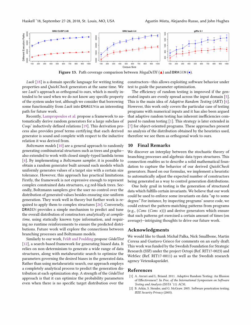
For our experiments, we use the coveragemeasure known asexecution path employed by American Fuzzy Lop (AFL) [20]—awell known fuzzer. It was chosen in this work since it is alsoused in the work by Grieco et al. [14] to compare MegaDeTHwith other techniques. The process consists of the instrumen-tation of the binaries under test, making them able to returnthe path in the code taken by each execution. Then, we useAFL to count how many different executions are triggered bya set of randomly generated files—also known as a corpus. Inthis evaluation, we compare how different QuickCheck genera-tors, derived using MegaDeTH and using our approach, resultin different code coverage when testing external programs,as a function of the size of a set of independently, randomlygenerated corpora. We have not been able to automaticallyderive such generators using Feat, since it does not work withsome Haskell extensions used in the bridging libraries.

We generated each corpus using the same ADTs and genera-tion sizes for each derivationmechanism.We used a generationsize of 10 for CLISP and bash files, and a size of 5 for Gif files.For , we used uniform cost functions to reduce anyexternal bias. In this manner, any observed difference in thecode coverage triggered by the corpora generated using eachderivation mechanism is entirely caused by the optimizationstage that our predictive approach performs, which does notrepresent an extra effort for the programmer. Moreover, werepeat each experiment 30 times using independently gener-ated corpora for each combination of derivation mechanismand corpus size.

Figure 13 compares the mean number of different executionpaths triggered by each pair of generators and corpus sizes,with error bars indicating 95% confidence intervals of themean.It is easy to see how the generators synthesize testcases capable of triggering a much larger number of different

execution paths in comparison toMegaDeTH ones. Our resultsindicate average increases approximately between 35% and41% with an standard error close to 0.35% in the number ofdifferent execution paths triggered in the programs under test.

An attentive reader might remember that MegaDeTH tendsto derive generators which produce very small test cases. If weconsider that small test cases should take less time (on average)to be tested, is fair to think there is a trade-off between beingable to test a bigger number of smaller test cases or a smallernumber of bigger ones having the same time available. How-ever, when testing external software like in our experiments, itis important to consider the time overhead introduced by theoperating system. In this scenario, it is much more preferableto test interesting values over smaller ones. In our tests, sizedifferences between the generated values of each tool does donot result in significant differences in the runtimes required totest each corpora—refer to the supplementary material for fur-ther details. A user is most likely to get better results by usingour tool instead of MegaDeTH , with virtually the same effort.

We also remark that, if we run sufficiently many tests, thenthe expected code coverage will tend towards 100% of thereachable code in both cases. However, in practice, our ap-proach is more likely to achieve higher code coverage for thesame number of test cases.

9 Related WorkFuzzers are tools to tests programs against randomly generatedunexpected inputs.QuickFuzz [13, 14] is a tool that synthesizesdata with rich structure, that is, well-typed files which can beused as initial “seeds” for state-of-the-art fuzzers—a work flowwhich discovered many unknown vulnerabilities. Our workcould help to improve the variation of the generated initialseeds, by varying the distribution of QuickFuzz generators—aninteresting direction for future work.

SmallCheck [27] provides a framework to exhaustively testdata sets up to a certain (small) size. The authors also proposea variation called Lazy SmallCheck, which avoids the genera-tion of multiple variants which are passed to the test, but notactually used.QuickCheck has been used to generate well-typed lambda

terms in order to test compilers [25]. Recently, Midtgaardet al. extend such a technique to test compilers for impureprogramming languages [22].


Figure 13. Path coverage comparison between MegaDeTH (▲) and (•).

Luck [18] is a domain specific language for writing testingproperties and QuickCheck generators at the same time. Wesee Luck’s approach as orthogonal to ours, which is mostly in-tended to be used when we do not know any specific propertyof the system under test, although we consider that borrowingsome functionality from Luck into is an interestingpath for future work.Recently, Lampropoulos et al. propose a framework to au-

tomatically derive random generators for a large subclass ofCoqs’ inductively defined relations [19]. This derivation pro-cess also provides proof terms certifying that each derivedgenerator is sound and complete with respect to the inductiverelation it was derived from.

Boltzmann models [10] are a general approach to randomlygenerating combinatorial structures such as trees and graphs—also extended to work with closed simply-typed lambda terms[4]. By implementing a Boltzmann sampler, it is possible toobtain a random generator built around such models whichuniformly generates values of a target size with a certain sizetolerance. However, this approach has practical limitations.Firstly, the framework is not expressive enough to representcomplex constrained data structures, e.g red-black trees. Sec-ondly, Boltzmann samplers give the user no control over thedistribution of generated values besides ensuring size-uniformgeneration. They work well in theory but further work is re-quired to apply them to complex structures [26]. Conversely,

provides a simple mechanism to predict and tunethe overall distribution of constructors analytically at compile-time, using statically known type information, and requir-ing no runtime reinforcements to ensure the predicted distri-butions. Future work will explore the connections betweenbranching processes and Boltzmann models.

Similarly to our work, Feldt and Poulding propose GödelTest[12], a search-based framework for generating biased data. Itrelies on non-determinism to generate a wide range of datastructures, along with metaheuristic search to optimize theparameters governing the desired biases in the generated data.Rather than using metaheuristic search, our approach employsa completely analytical process to predict the generation dis-tribution at each optimization step. A strength of the GödelTestapproach is that it can optimize the probability parameterseven when there is no specific target distribution over the

constructors—this allows exploiting software behavior undertest to guide the parameter optimization.The efficiency of random testing is improved if the gen-

erated inputs are evenly spread across the input domain [5].This is the main idea of Adaptive Random Testing (ART) [6].However, this work only covers the particular case of testingprograms with numerical inputs and it has also been arguedthat adaptive random testing has inherent inefficiencies com-pared to random testing [1]. This strategy is later extended in[7] for object-oriented programs. These approaches presentno analysis of the distribution obtained by the heuristics used,therefore we see them as orthogonal work to ours.

10 Final RemarksWe discover an interplay between the stochastic theory ofbranching processes and algebraic data types structures. Thisconnection enables us to describe a solid mathematical foun-dation to capture the behavior of our derived QuickCheckgenerators. Based on our formulas, we implement a heuristicto automatically adjust the expected number of constructorsbeing generated as a way to control generation distributions.One holy grail in testing is the generation of structured

data which fulfills certain invariants. We believe that our workcould be used to enforce some invariants on data “up to somedegree.” For instance, by inspecting programs’ source code, wecould extract the pattern-matching patterns from programs(e.g., (Cons (Cons x))) and derive generators which ensurethat such patterns get exercised a certain amount of times (onaverage)—intriguing thoughts to drive our future work.

AcknowledgmentsWe would like to thank Michał Pałka, Nick Smallbone, MartinCeresa and Gustavo Grieco for comments on an early draft.This work was funded by the Swedish Foundation for StrategicResearch (SSF) under the project Octopi (Ref. RIT17-0023) andWebSec (Ref. RIT17-0011) as well as the Swedish researchagency Vetenskapsrådet.

References[1] A. Arcuri and L. Briand. 2011. Adaptive Random Testing: An Illusion

of Effectiveness?. In Proc. of the International Symposium on SoftwareTesting and Analysis (ISSTA ’11). ACM.

[2] B. Arkin, S. Stender, and G. McGraw. 2005. Software penetration testing.IEEE Security Privacy (2005).


[3] T. Arts, J. Hughes, U. Norell, and H. Svensson. 2015. Testing AUTOSARsoftware with QuickCheck. In In Proc. of IEEE International Conferenceon Software Testing, Verification and Validation, ICST Workshops.

[4] M. Bendkowski, K. Grygiel, and P. Tarau. 2017. Boltzmann Samplersfor Closed Simply-Typed Lambda Terms. In In Proc. of InternationalSymposium on Practical Aspects of Declarative Languages. ACM.

[5] F.T. Chan, T.Y. Chen, I.K. Mak, and Y.T. Yu. 1996. Proportional samplingstrategy: guidelines for software testing practitioners. Information andSoftware Technology 38, 12 (1996), 775 – 782.

[6] T. Y. Chen, H. Leung, and I. K. Mak. 2005. Adaptive Random Testing.In Advances in Computer Science - ASIAN 2004. Higher-Level DecisionMaking, Michael J. Maher (Ed.). Springer Berlin Heidelberg.

[7] I. Ciupa, A. Leitner, M. Oriol, and B. Meyer. 2008. ARTOO: adaptiverandom testing for object-oriented software. In Proc. of InternationalConference on Software Engineering. ACM/IEEE.

[8] K. Claessen, J. Duregård, and M. H. Palka. 2014. Generating ConstrainedRandom Data with Uniform Distribution. In Proc. of the Functional andLogic Programming FLOPS.

[9] K. Claessen and J. Hughes. 2000. QuickCheck: A Lightweight Tool forRandom Testing of Haskell Programs. In Proc. of the ACM SIGPLANInternational Conference on Functional Programming (ICFP).

[10] P. Duchon, P. Flajolet, G. Louchard, and G. Schaeffer. 2004. BoltzmannSamplers for the Random Generation of Combinatorial Structures. Com-binatorics, Probability and Computing. 13 (2004).

[11] J. Duregård, P. Jansson, andM.Wang. 2012. Feat: Functional enumerationof algebraic types. In Proc. of the ACM SIGPLAN Symposium on Haskell.

[12] R. Feldt and S. Poulding. 2013. Finding test data with specific propertiesvia metaheuristic search. In Proc. of International Symp. on SoftwareReliability Engineering (ISSRE). IEEE.

[13] G. Grieco, M. Ceresa, and P. Buiras. 2016. QuickFuzz: An automaticrandom fuzzer for common file formats. In Proc. of the InternationalSymposium on Haskell. ACM.

[14] G. Grieco, M. Ceresa, A. Mista, and P. Buiras. 2017. QuickFuzz testingfor fun and profit. Journal of Systems and Software 134, Supp. C (2017).

[15] P. Haccou, P. Jagers, and V. Vatutin. 2005. Branching processes. Variation,growth, and extinction of populations. Cambridge University Press.

[16] J. Hughes, C. Pierce B, T. Arts, and U. Norell. 2016. Mysteries of DropBox:Property-Based Testing of a Distributed Synchronization Service. In Proc.

of the Int. Conference on Software Testing, Verification and Validation,ICST.

[17] J. Hughes, U. Norell, N. Smallbone, and T. Arts. 2016. Find more bugswith QuickCheck!. In Proc. of the International Workshop on Automationof Software Test, AST@ICSE.

[18] L. Lampropoulos, D. Gallois-Wong, C. Hritcu, J. Hughes, B. C. Pierce, andL. Xia. 2017. Beginner’s luck: a language for property-based generators.In Proc. of the ACM SIGPLAN Symposium on Principles of ProgrammingLanguages, POPL.

[19] L. Lampropoulos, Z. Paraskevopoulou, and B. C. Pierce. 2017. GeneratingGood Generators for Inductive Relations. In Proc. ACM on ProgrammingLanguages 2, POPL, Article 45 (2017).

[20] M. Zalewski. 2010. American Fuzzy Lop: a security-oriented fuzzer.http://lcamtuf.coredump.cx/afl/. (2010).

[21] C. McBride and R. Paterson. 2008. Applicative Programming with Effects.Journal of Functional Programming 18, 1 (Jan. 2008).

[22] J. Midtgaard, M. N. Justesen, P. Kasting, F. Nielson, and H. R. Nielson.2017. Effect-driven QuickChecking of compilers. In Proceedings of theACM on Programming Languages, Volume 1 ICFP (2017).

[23] A. Mista, A. Russo, and J. Hughes. 2018. Branching Processes forQuickCheck Generators (extended version). https://bitbucket.org/agustinmista/dragen/downloads/full-paper.pdf. (2018).

[24] N. Mitchell. 2007. Deriving Generic Functions by Example. In Proc. ofthe 1st York Doctoral Syposium. Tech. Report YCS-2007-421, Departmentof Computer Science, University of York, UK, 55–62.

[25] M. Pałka, K. Claessen, A. Russo, and J. Hughes. 2011. Testing and Optimis-ing Compiler by Generating Random Lambda Terms. In The IEEE/ACMInternational Workshop on Automation of Software Test (AST 2011).

[26] S. M. Poulding and R. Feldt. 2017. Automated Random Testing in MultipleDispatch Languages. IEEE International Conference on Software Testing,Verification and Validation (ICST) (2017).

[27] C. Runciman, M. Naylor, and F. Lindblad. 2008. Smallcheck and LazySmallcheck: automatic exhaustive testing for small values. In Proc. of theACM SIGPLAN Symposium on Haskell.

[28] T. Sheard and Simon L. Peyton Jones. 2002. Template meta-programmingfor Haskell. SIGPLAN Notices 37, 12 (2002), 60–75.

[29] H. W. Watson and F. Galton. 1875. On the probability of the extinctionof families. The Journal of the Anthropological Institute of Great Britainand Ireland (1875).

http://lcamtuf.coredump.cx/afl/

https://bitbucket.org/agustinmista/dragen/downloads/full-paper.pdf

https://bitbucket.org/agustinmista/dragen/downloads/full-paper.pdf

branching processes for quickcheck generatorsrusso/publications_files/haskell2018.pdf · megadeth...

Documents