BOWHEAD WHALE FEEDING ECOLOGY STUDY (BOWFEST) 

IN THE WESTERN BEAUFORT SEA  

2009 Annual Report  

       

A project provided to: Environmental Studies Program Alaska Outer Continental Shelf Region Minerals Management Service 94 East 36th Avenue, 3rd Floor Anchorage, Alaska 99508-4363

Submitted through: National Marine Mammal Laboratory Alaska Fisheries Science Center, F/AKC4 7600 Sand Point Way, NE, Seattle WA 98115-0070 Phone: 206-526-4018; FAX 206-526-6615

1 

 

2 

 

TABLE OF CONTENTS

INTRODUCTION . . . . . . . . 3 SECTION I - AERIAL SURVEYS OF BOWHEAD WHALES IN THE VICINITY OF BARROW

AUGUST-SEPTEMBER 2009 Goetz, Rugh, Mocklin . . . . . . 4

SECTION II - PASSIVE ACOUSTIC MONITORING IN THE WESTERN BEAUFORT SEA

Berchok, Stafford, Mellinger, Moore, George . . . 22 SECTION III - MOORING AND BROAD-SCALE OCEANOGRAPHY . . . 38

SHORT-TERM MOORINGS Okkonen . . . . . . . 38

BROAD-SCALE OCEANOGRAPHY COMPONENT Ashjian, Campbell, Okkonen . . . . 41

SECTION IV - TAGGING AND FINE-SCALE OCEANOGRAPHY

Baumgartner . . . . . . . 45

SECTION V - NORTH SLOPE BOROUGH RESEARCH . . . . 51 LOCAL BOAT-BASED BOWHEAD WHALE SURVEYS

George . . . . . . . 52 STOMACH EXAMINATIONS

George, Sheffield  .  .  .  .  .  .  54 

BOWFEST PRESENTATIONS AND MEETINGS IN 2009 . . . 62

3 

 

 BOWHEAD WHALE FEEDING ECOLOGY STUDY 

(BOWFEST) Annual Report for 2009 

 INTRODUCTION 

The Bowhead Whale Feeding Ecology Study (BOWFEST) was initiated in May 2007

through an Interagency Agreement between the Minerals Management Service (MMS) and the National Marine Mammal Lab (NMML). The study is being conducted through grants and contracts to scientists at Woods Hole Oceanographic Institute (WHOI), University of Rhode Island (URI), University of Alaska Fairbanks (UAF), University of Washington (UW), Oregon State University (OSU), as well as through employees at NMML. Field work is being coordinated with the North Slope Borough (NSB), Alaska Eskimo Whaling Commission (AEWC), Barrow Whaling Captains' Association (BWCA), Alaska Department of Fish and Game (ADFG), and MMS. Marine mammal studies are as permitted under NMML’s Permit No. 782-1719.

This study focuses on late summer oceanography and prey densities relative to bowhead whale (Balaena mysticetus) distribution over continental shelf waters between the coast and 72°N and between 152º -157º west longitudes, which is north and east of Point Barrow, Alaska. Aerial surveys and acoustic monitoring provide information on the spatial and temporal distribution of bowhead whales in the study area. Oceanographic sampling helps identify sources of zooplankton prey available to whales on the continental shelf and the association of this prey with physical (hydrography, currents) characteristics which may affect mechanisms of plankton aggregation. Prey distribution will be better understood by examining temporal and spatial scales of the hydrographic and velocity fields in the study area, particularly relative to frontal features. Results of this research program may help explain increased occurrences of bowheads feeding in the Western Beaufort Sea (US waters), well west of the typical summer feeding aggregations in the Canadian Beaufort Sea. Increased understanding of bowhead behavior and distribution is needed to minimize potential impacts from petroleum development activities.

The following reports describe field work and the respective analyses conducted under BOWFEST funds in 2009. This is the second of three proposed years of field work for this program.

4 

 

SECTION I - AERIAL SURVEYS OF BOWHEAD WHALES IN THE VICINITY OF BARROW AUGUST-SEPTEMBER 2009

Kimberly T. Goetz, David J. Rugh, and Julie A. Mocklin

National Marine Mammal Laboratory

Alaska Fisheries Science Center National Marine Fisheries Service, NOAA

7600 Sand Point Way NE Seattle, Washington 98115

Abstract

The aerial survey component of BOWFEST is designed to document patterns and variability in the timing and locations of bowhead whales as well as provide an estimate of temporal and spatial habitat use. In addition, aerial photography provides information on residence times (through reidentification of individual animals) and sizes of whales (through photogrammetry). With the consideration of acoustic mooring locations, preset oceanographic transects, bathymetric gradients, and distance from the base of operations (Barrow), a two-part study area and aerial trackline sampling scheme was devised. Using a NOAA Twin Otter, scientists from the National Marine Mammal Laboratory (NMML) conducted aerial surveys from 29 August-18 September 2009 over continental shelf waters from 157° W to 152° W and from the coastline to 72° N, with most of the effort concentrated between 157° W and 154° W and between the coastline and 71° 44’N. There were 25 sightings of bowheads (an estimated 52 whales) during 18.0 flight hours (approximately a quarter of the 76 available flight hours; the survey was greatly limited due to fog and high winds). Most of these sightings were near the 20 m isobath. Two Canon EOS-1DS Mark III cameras were used for photography; 245 pictures were taken with a 55 mm lens for photogrammetry, and 186 pictures were taken with a 70-200 mm lens for photo-identification. Unlike in 2007 when nearly all bowheads appeared to be feeding as indicated by mud plumes and multiple swim directions, in 2008 and 2009 aerial observers identified only 4 of the 56 and 5 of the 25 bowhead sightings as feeding. Examination of the photographs will provide more precise records of how many whales were feeding as evidenced by mud on the body, open-mouths, and the presence of feces. “Traveling” was the most commonly recorded behavior, indicating that bowheads were most likely migrating through the study area. Collecting additional years of data as well as integrating aerial information with other projects will help elucidate the extent to which bowheads feed near Point Barrow in the summer.

Introduction

Most bowhead whales of the Bering-Chukchi-Beaufort (BCB) stock migrate annually from the Bering Sea, through the Chukchi Sea, to the eastern Beaufort Sea. During the spring migration, bowheads typically arrive in the Barrow area in early April, and the population continues migrating past Barrow until mid-June. By early September, bowheads start leaving the

5 

 

eastern Beaufort Sea, traveling northwesterly towards Barrow and west across the Chukchi Sea throughout September and October (Moore & Reeves 1993). Although bowheads are more commonly seen off Barrow during the spring and autumn migrations, there have also been reports of whales feeding near Barrow in summer (July to September). There is no documentation as to whether these animals are still traveling from the Chukchi Sea following the spring migration, traveling towards the Chukchi Sea prior to the autumn migration, or residing between the Chukchi and Beaufort seas throughout the summer. BOWFEST was established to determine the scale of feeding near Barrow in the summer and the consistency of this behavior relative to location within the study area, year, and age class (using whale size as a proxy for age). In addition, the ecological relationship between feeding bowhead whales and relevant oceanographic parameters -- such as bathymetry, currents, temperatures, and ice conditions -- are being examined to assess whether oceanographic features indirectly affect the location of bowhead feeding aggregations by influencing prey distribution. Accordingly, the aerial survey component of BOWFEST will document patterns and variability in the timing and locations of bowhead whales as well as provide an estimate of temporal and spatial habitat use. In addition, aerial photography provides information on residence times (through reidentification of individual animals) and sizes of whales (through photogrammetry).

Methods

Study Area and Trackline Design Based on the survey scheme designed in 2007, a two-part study area and aerial trackline sampling scheme was devised. The extent of the study area covered continental shelf waters from 157° W to 152° W and from the Alaska coastline to 72° N (Figure I-1). The inner section of the study area (yellow) was 7,276 km2, and the larger, outer section (green) was 12,152 km2.

Five years of data (2000-2005) from the Bowhead Whale Aerial Survey Project (BWASP), operated by Minerals Management Service (MMS), were used to calculate bowhead whale density (whales per unit effort) within the BOWFEST study area. This helped to stratify and ultimately to determine the distribution and quantity of survey effort relegated to each section. According to the BWASP data, the density of bowhead whales in the inner section was approximately six times greater than the larger section of the study area. Using equations 7.1, 7.2, and 7.4 from Buckland et al. (1993), we calculated the total effort needed in each of the two sections of the BOWFEST study area to obtain a detection probability sufficient for determining relative densities of whales. Since oceanographic data becomes more difficult to collect with increased distance away from Barrow and much of the intent of BOWFEST is to compare ecological parameters relative to whale distribution, we arbitrarily decreased the effort for the larger section to keep our main focus on the inner area with more overlap of the whales and other BOWFEST researchers. Trackline orientation was based on the pre-determined oceanographic tracklines which ran in a northeasterly direction at approximately 66° True, approximately perpendicular to the coast.

Figure I-1. Two-part study area (inner yellow section and outer green section) relative to pre-set oceanographic tracklines (purple) and acoustic moorings.

Line transect methodology described in Buckland et al. (1993) was utilized to calculate total survey effort for each section of the study area based on available survey hours for this project. Sampling schemes consisted of shifting the trackline array short distances to the east or west, removing the likelihood that any tracklines would be flown twice within a season. The entire study area contained approximately 5,011 km of trackline, 3,554 km in the inner section and 1,457 km in the outer section (Fig. I-2). Based on the allocation of effort and the flight hours available, the tracklines in the inner section were spaced 2 km apart while lines in the outer section were spaced 8 km apart. The placement of the first survey line in the inner section of the study area (closer to Barrow) was determined by random selection. In 2009, the first transect line was placed 1.5 km from the northwest corner of the inner and outer portions of the study area. We purposely used the same random value (1.5 km) to calculate placement of the first line in both sections of the study area in order to align the tracklines in the outer study area with the tracklines in the inner study area. This method, simplified flight logistics and minimized transit time between tracklines. Subsequent tracklines were parallel to the first trackline and spaced 2 km apart for the inner area and 8 km apart for the outer area.

6 

 

Figure I-2. Two-part study area with tracklines designed for the 2009 BOWFEST aerial survey.

In order to prevent overlap in survey effort due to tightly spaced tracklines, four sampling schemes were devised (Fig. I-3). The first scheme (Scheme 1) was created by selecting the first line from the west side of the study area and every fourth line thereafter. Using the same method, beginning with the second through fourth lines from the west side of the study area, the three remaining schemes were created. As a result, tracklines were spaced approximately 8 km and 32 km apart in the inner and outer sections of the study area, respectively (Fig. I-3). Survey Protocol

BOWFEST aerial surveys were flown in a NOAA Twin Otter (N57RF) equipped with twin engines, high wings, and more than 6 hours of flying capacity. In addition, the aircraft had 2 large bubble windows for the left and right observers and an open belly window/camera port for vertical photography. An intercom system allowed communication among observers, pilots, and data recorder while a VHF radio allowed communication with vessels, such as when reporting whale locations. A laptop computer, interfaced with a custom built aerial survey program and a portable Global Positioning System (GPS – Garmin 76 CSx) recorded sighting position, weather, effort (on or off), crew position, and photo data into an Access database. Location data (latitude, longitude, speed, altitude, and heading) were automatically recorded every five seconds; all other entries were entered manually. In addition, each start and stop of a transect leg was recorded. Specific data entries for weather included overall percent ice cover, ice type (categorized using the Observers Guide to Sea Ice http://response.restoration.noaa.gov/book_shelf/695_seaice.pdf), sky condition, and sea state (on a Beaufort scale) as well as glare, visibility angle, and visibility quality for each side of the aircraft. Observers used an inclinometer (0° = horizontal; 90° =

7 

 

Figure I-3. The four survey schemes for the 2009 BOWFEST aerial survey.

straight down) to accurately determine the searchable distance out each side of the aircraft. Visibility quality within the given inclinometer angle was documented as the best of one of five subjective categories from excellent to useless; for example, a record of “20° good” would mean that from the trackline out to 20° (0.8 km), sighting opportunities were good, and farther from the trackline (<20°) the visibility worsened and was not recorded. Areas along the trackline where observers rated visibility quality as poor or useless on both sides of the aircraft were considered off effort and, thus, unsurveyed. Date, time, sighting observer, inclinometer angle, group size, and species were recorded for all marine mammals; in addition, for large whale sightings, observers reported calf number, travel direction, sighting cue, dominant behavior, group composition, reaction to plane, and number of nearby vessels.

Survey altitude was generally near 310 m (1000 ft); most aerial photographic passes were made at 230 m (750 ft), as allowed under NMML Permit No. 782-1719-09. The northeast/southwest tracklines were flown sequentially west to east (opposite the bowhead whales’ autumn migration direction) in order to minimize the probability of resighting the same whale(s).

Immediately upon sighting a marine mammal, each observer reported the group size and species to the data recorder. As the aircraft passed abeam of the sighting, the observer informed

8 

 

the recorder of an inclinometer angle and whether or not there was an observable reaction to the aircraft. The plane deviated from the trackline only when an observer reported an unidentified large cetacean sighting (in order to obtain an adequate identification). After a bowhead was reported, the trackline was typically completed before going off effort to begin photographic passes. This method allowed for a routine reporting of bowhead whales on the trackline and minimized confusion in reporting sightings while off-effort.

Photographic Protocol

Two Canon EOS-1DS Mark III cameras were used simultaneously over an open belly port for vertical photography (Fig. I-4A). A 70-200 mm lens (usually set at 200 mm) was used to provide larger images of whales for purposes of identifying individual animals. This lens was equipped with image stabilization technology and was set to autofocus throughout the survey. Since this camera was held vertically over the belly port , the images can also be used to obtain relative whale lengths in the event that a whale was not captured by the photogrammetry camera (Fig. I-4B).

The second camera, with a 55 mm fixed lens (no magnification), was used for photogrammetry in order to best estimate whale lengths. This lens was focused to infinity and taped to impede rotation. The camera was housed in a Forward Motion Compensation (FMC) mount (installed on the left side of the belly port) which uses a rocker mechanism to counter the forward velocity of the relative ground speed. The camera was integrated with an autonomous radar altimeter (Honeywell AA300 model) in order to collect precise altitudes each time the camera was fired (http://www.aerialimagingsolutions.com/fmcmount.html; Fig. I-4C). Unlike the handheld camera for photo-identification, this mounted camera was fired using a custom built data acquisition system that automated the retrieval of data including altitude, time of camera firing, frame number, aircraft speed, and focal length of the camera lens. Immediately prior to a whale appearing beneath the plane, a keystroke on the computer triggered the camera to continuously fire so that each consecutive image overlapped the previous photo by 60%, adjusted for altitude. Both cameras recorded RAW format, 21.0 megapixels (5616 x 3744) images and were set to shutter priority, 800 ISO sensitivity (or lower), and 1/1000s or faster shutter speed.

Photo by Dave Rugh, 2008 Photo by Dave Rugh, 2008

Figure 4. A) The NOAA Twin Otter (N57RF) with open belly port. B) The handheld Canon EOS-1DS Mark III with 70-200 mm lens used for photo-identification. C) The

 Belly Port A.

Photo by Craig George, 2008

 B.

 C.Figure I-4. A) The NOAA Twin Otter (N57RF) with open belly port. B) The handheld Canon

EOS-1DS Mark III with 70-200 mm lens used for photo-identification. C) The Canon EOS-1DS Mark III with 55 mm lens housed in the FMC mount on the left side of the belly port.

9 

 

Photographic passes were typically made after completing the trackline on which the bowhead sighting was initially reported. After breaking trackline effort, a single pass was made directly over the bowhead group in order to obtain a precise location. Several additional passes were flown over each group until the observers felt that most whales in the area had been photographed. During each photographic pass, the forward observer provided a countdown to alert the photographer(s) when a whale was about to appear under the aircraft. In addition to photographing bowhead whales, photographs were taken of two calibration targets (one over land and the other over water) using the same two cameras (Canon EOS-1DS Mark III) and lenses (55 mm and 70-200 mm). The land target, provided by Craig George, North Slope Borough (NSB), consisted of painted 2" x 10" boards with precisely measured intervals that were visible at survey altitude (1000 ft) (Fig. I-5). The calibration target was laid out on an abandoned airstrip north of Barrow near the former Naval Arctic Research Lab’s aircraft hangar.

   

5

18

12

0

3

5

4

10 34

8

10

12

15

0

NORTH

DD

c cc caa

bb

Figure I-5. Aerial image (left) and diagram (right) of the land-based calibration target.

A second, floating water target was developed by David Rugh, Julie Mocklin, and Noah

Lawrence-Slavas in order to detect possible discrepancies between radar altimeter performance over land and water. The target consisted of 200 ft non-stretch rope attached to an array of floats (4 large and 1 small) followed by a 36 inch drogue needed to keep the line straight and reduce undulations (Fig. I-6). The drogue was attached to the rope by a 5/16” swivel to allow free rotation. This apparatus was then towed by a 27-foot motorboat in a lagoon not far from Barrow where sea surface conditions were fairly calm.

10 

 

Figure I-6. Aerial photograph of the 27-foot motor boat towing the water-borne calibration target in Elson Lagoon in 2009.

To test the performance of the autonomous radar altimeter, photographs of both calibration targets were taken at 100 ft intervals from 500 to 1000 ft. Since the lengths between marks on the targets are known precisely, altimeter readings can be corrected. This correction factor can then be applied to photographs of bowhead whales to provide more accurate body length estimates. Vertical photography removes angle as a variable when applying aircraft altitude to the calculation of distance between the camera and the target.

After each survey, all photographs were geo-referenced using RoboGEO. The GPX file was downloaded from the GPS unit and RAW images were converted to TIFFs. Both the GPX file and the TIFFs were used as inputs for RoboGEO so that the program could interpolate latitude and longitude and embed this position information in the exif data of each photograph. Since RoboGeo uses time to link photographs to the tracklog position, we synchronized the date and time on both cameras with the date and time on the GPS unit at the beginning of each survey. Once geo-referenced, all images and associated metadata were sent to LGL for analysis of whale lengths.

Processing images for photo-identification of individual whales begins with cropping and labeling images into a standard format. These images are then archived in the large collections maintained by NMML and LGL. Each whale image is categorized according to identifiability, and the photo is quality-rated according to an established protocol (Rugh et al. 1998). All images will be compared to each other to determine if some individual whales were photographed multiple times. Following this comparison, these whale images will be compared to others collected in previous years to establish when and where individual whales have been seen before.

Results

Survey effort Aerial surveys were conducted in the BOWFEST study area on 5 days between 29 August

and 18 September 2009. All flights were based out of Barrow, each ranging from 1.0 to 5.7 hours in duration. Although 76 flight hours were originally scheduled for the project, fog, low ceilings, and high winds limited flying conditions on many days such that only 18.0 hours (3,449 km) were flown. Of the 13.1 hours spent on search effort over water, 5.4 hours (1,007 km) were flown on systematic transects and 7.3 hours (1,377 km) were flown searching off transects such as when transiting between transect lines, circling animals, or photographing whales (Figures I-

11 

 

7A & 7B). An additional 2.3 hours were spent flying over and photographing calibration targets, and 1.3 hours was spent deadheading or on transect without search effort (Table I-1). Due to logistical difficulties (fuel limitations and weather), the boat crews collecting oceanographic samples and tagging whales typically did not travel long distances from Barrow. As a result, the aerial surveys were concentrated in the inner section of the two-part study area with no search effort in the outer section.

Throughout the entire 2009 BOWFEST field season, only 1.2 hours (250 km) were flown in poor or useless viewing conditions and, thus, were considered unsurveyed (Table I-1). The 1.2 hours does not take into consideration the numerous times we changed course, deviated from transects, or altered our elevation to avoid low ceilings, precipitation, or fog. In addition, on 16 of the possible 21 survey days, poor weather conditions precluded us from flying.

 

Figure I-7. A) All search effort, including transect, circling, and photo effort; and B) dedicated transect effort during the 2009 BOWFEST survey.

Table I-1. Survey effort (distance and time) for the 2009 BOWFEST aerial survey.

12 

 

EFFORT SUMMARY DISTANCE (KM) TIME (HRS)On Effort - Trackline 1007.01 5.39On Effort - Deadhead 624.54 3.26On Effort - Photo Mode 435.05 2.38On Effort - Circling 317.61 1.69Total On Effort 2384.21 12.72

Total Off Effort 623.49 2.99

Totals 3449.41 18.03

Off Effort - Over Land 85.91 0.45Off Effort - Bad Weather 249.85 1.23Off Effort - Deadhead 279.26 1.27Off Effort - Trackline 8.48 0.05

Calibrating Targets 441.70 2.32

 

Two of the four devised survey schemes (Schemes 1 and 2) were flown during the 2009 BOWFEST survey. Only tracklines in the inner section of the study area were flown this season primarily due to poor weather conditions which limited flight time. Additionally, priority was to survey the inner section because that is where boat-based operations were being conducted. Approximately 782 km of transects were flown in Scheme 1 (63%) on 2 and 4 September, and an additional 905 km were flown on effort while circling, photographing, or transiting between tracklines (Table I-2; Fig. I-8). Scheme 2 was attempted three times, once each on 7, 14, 15 September, covering approximately 18% of the Scheme. Of the 2503 km of designated trackline within Schemes 1 and 2, only 40% were completed. Schemes 3 and 4 were not flown.

Table I-2. Search effort per survey scheme in 2009.

13 

 

Flight Scheme

Transects Availible (km)

% Transects flown

1 904.6 289.1 782.3 250.5 1251.6 62.52 472.6 150.8 224.7 72.8 1251.4 18.0

Off Transects km mins

On Transects km mins

Totals 1377.2 439.9 1007.0 323.3 2503.0 40.2

 

Photographic effort

Figure I-8. Aircraft tracklines (black lines) per survey scheme (colored lines) flown during the 2009 BOWFEST field season. Only 2 of the 4 schemes were flown. Scheme 1 is depicted on the left, and Scheme 2 is on the right.

Bowhead whales were photographed on two of the five survey days. In total, we spent 2.4 hours (435 km) photographing bowheads, resulting in 50 pictures (53 bowhead images) for photogrammetry (PGRAM) and 58 pictures (63 bowhead images) for photo-identification (PID) (Table I-3; Fig. I-9). An additional 297 pictures were taken of the land and water calibration targets (190 pictures using the photogrammetry camera and 107 using the photo-identification camera). Although there were 116 bowhead whales counted on a total of 108 photographs, the number of unique bowhead whales will be less after accounting for duplicate images.

Date Method* Bowhead Pictures

Bowhead Images**

Calibration Pictures

PGRAM 39 42PID 42 47PGRAM 11 11PID 16 16PGRAM 0 0 132PID 0 0 107PGRAM 0 0 58PID 0 0 0

14 

 

Total 108 116 297

7-Sep

15-Sep

2-Sep

4-Sep

Table I-3. Photographic effort for the 2009 BOWFEST aerial survey.

** * PGRAM = Photogrammetry, PID = Photo-identification

** Total number of individual bowheads counted from all pictures (e.g. one picture may have 3 or more bowhead images).

Figure I-9. Locations where bowhead whales were photographed per survey day (2 and 4 Sept. 2009) in the left figure; and photographic locations (black circles) relative to all bowhead sightings made during these aerial surveys in 2009 (red stars) in the right figure.

Sighting Summary There were 25 bowhead sightings of 37 animals seen throughout the 2009 BOWFEST

survey. After breaking trackline to circle/photograph the whales, an additional 15 animals were counted, bringing the total number of bowheads to 52 (Table I-4). Unlike the 2007 field season, when nearly all bowheads appeared to be feeding as indicated by mud plumes and multiple swim directions, only 5 of the 25 bowhead sightings were positively identified as feeding in 2009. (Examination of the photographs will later document how many bowheads had mud on their bodies, and therefore were probably feeding). This observed behavior was similar to 2008 in which “traveling” was the most commonly recorded behavior, indicating that bowheads were most likely migrating through the study area, perhaps feeding along the way. The most bowhead

whale sightings were made on 2 September (5 sightings of 15 animals) and 4 September (5 sightings of 19 animals) (Figs. I-10 and I-11). Figure I-12 shows that the majority of survey effort on the five survey days was completed during relatively calm sea states (Beaufort ≤ 3).

15

19

5

13

0

2

4

6

8

10

12

14

16

18

20

2-Sep 4-Sep 7-Sep 15-Sep

Bow

head

s

2009 Survey Days

# of Bowheads Counted # of Bowhead Sightings  

Figure I-10. Number of bowhead

sightings (yellow triangles) and bowheads counted (green bars) per survey day in 2009. Counts may include resightings between days.

0

200

400

600

800

1000

1200

2-Sep 4-Sep 7-Sep 15-Sep

Sea

rch

Eff

ort i

n K

ilom

eter

s

2009 Survey Days

B0 B1 B2 B3 B4 B5 B6 B7  

Figure I-11. Search effort per survey day categorized by Beaufort sea state (B).

15 

 

In addition to bowhead whales, there were 22 sightings of gray whales (30 whales), 1 sighting of a single humpback whale, 2 sightings of ringed seals (2 seals), 6 sightings of bearded seals (6 seals), 3 sightings of 12 walrus, 22 sightings of unidentified seals (43 animals), 3 sightings of unidentified pinnipeds (9 animals), and 6 sightings of unidentified large cetaceans (7 animals) (Table I-4, Fig. I-13). The frequent encounter of high sea states and relatively high survey altitude (1000 ft) made identifying seals to species level difficult, resulting in a large number of unidentified seals.

16 

 

Table I-4. Summary of marine mammal sightings and numbers of marine mammals counted during the 2009 BOWFEST aerial survey. The counts with asterisks (*) include whales seen while the aircraft was circling and not on transects.

 

Common Name Scientific Name Sightings CountBowhead Whale Balaena mysticetus 25 37 (52*)Gray Whale Eschrichtius robustus 22 30Humpback Whale Megaptera novaeangliae 1 1Unid Large Cetacean 6 7Ringed Seal Phoca hispida 2 2Bearded Seal Erignathus barbatus 6 6Walrus Odobenus rosmarus 3 12Unid Pinniped 3 9Unid Seal 22 43

90 14 (162*) 

Figure I-13. Map with zoomed inset showing locations of all marine mammal sightings.

17 

 

2009 Daily Reports August 28 Aerial photogrammetric equipment (FMC mount, camera, autonomous altimeter, and interfacing equipment) was installed in Anchorage using the FAA hangar. The floating calibration targets were assembled in Barrow along with other pre-survey preparations. August 29 The full aerial survey team and aircraft are in Barrow by 15:00. Weather was poor, so there was no attempt to fly. August 30 Field equipment is installed on the aircraft, aerial operations are refined, and the crew has a safety briefing. Winds are too strong (40 knots) to attempt to fly. August 31 Winds are 26-36 knots and rising with gale warnings plus sleet and snow, so no flight was attempted. September 1

There was no flight today due to a scheduled pilot down day. In addition, high winds (25-30 knots) and low ceilings were not conducive for flying. The aerial survey team took advantage of the downtime by making sure all programs were running smoothly.

September 2

The first flight (Flight 1) for BOWFEST in 2009 was 5.7 hour (1,072 km) and used tracklines from Scheme 1. We began with the northwestern most tracklines and proceeded westward. After completing four tracklines, a whale was seen near Point Barrow; it was circled several times but could not be identified. Midway up the fifth trackline, we saw an aggregation of whales consisting of 5 gray whales, 1 bowhead whale (group 1), and a single humpback whale. Three more tracklines were completing before making two bowhead whale sightings (groups 2 and 3). After completing photographic passes, we continued on tracklines before sighting more bowheads (group 4). As with the previous groups, we flew several photographic passes over group 4 and completed an additional trackline to the east before heading back to Barrow. On Flight 1, we spent approximately 93 minutes photographing bowheads, collecting 81 photographs (42 for photo-identification and 39 for photogrammetry). Most of the survey was completed with fairly calm sea states (Beaufort<4).

In addition to bowhead, gray, and humpback whale sightings, there were also 2 ringed seal sightings (2 animals), 4 bearded seal sightings (4 animals), 2 walrus (7 animals), 17 unidentified seal sightings (38 seals), 2 unidentified pinniped sightings, and one unidentified large cetacean sighting of a single whale. September 3

Gale force winds (25-35 knots) and rain precluded flying on this day.

18 

 

September 4 Winds dropped sufficiently that we were able to conduct a survey on this day (Flight 2).

Because the westernmost tracklines in the smaller section of the study area were previously flown, we deadheaded to the easternmost trackline and flew lines west until all tracklines on Scheme 1 were completed (between Flights 1 and 2). While transiting between tracklines, we sighted the first group of bowheads (group 1; 7 animals). After completing several photographic passes, we completed two more tracklines before finding another group of bowhead whales (group 2; 2 animals). Due to the small number of animals in group 2, we did not break trackline for photographic passes. Two more tracklines to the west were flown before encountering the third group of animals (group 3; 5 animals). Several photographic passes were made over this group before resuming trackline effort. While transiting to the next trackline, a fourth group of bowhead whales was sighted (group 4; 4 animals), but no photographic passes were attempted because the water was opaque, and only a small portion of each whale was visible. We were able to complete one additional trackline before heading back to Barrow. An additional bowhead (group 5; 1 animal) was sighted during the return flight. During the 4.3 hour flight, 50 minutes were spent photographing bowhead whales, collecting a total of 27 photos (11 for photogrammetry and 16 for photo-identification). Ceilings were variable throughout the survey with moderate wind causing sea states to range from Beaufort 2 to 5. Other than the 19 bowhead whales, no other marine mammals were sighted, probably because pinnipeds are only visible in the best viewing conditions. September 5-6

There were no flights these days due to high winds, sometimes up to 30 knots, high sea states, and low ceilings. In addition, it was decided to schedule 6 September as a pilot down day, to take advantage of a poor weather day and “re-set” the pilots’ schedule for time off. September 7

Conditions were good enough for a survey on this day (Flight 3). The primary goal of this flight was to photograph calibration targets on land and water. We began Flight 3 by completing two of the westernmost tracklines on Scheme 2 before breaking effort to photograph the calibration targets. We collected 156 photographs while flying photographic passes over a floating calibration target north of Point Barrow being pulled by Little Whaler and a land-based target on the abandoned runway north of NARL. On the transit to the land calibration target located near Barrow, we encountered a productive area with gray whales (25 animals), bowhead whales (5 animals), and three unidentified large cetaceans. Several passes were made over this area for videotaping purposes, so the number of animals counted may include repeats. Viewing conditions were generally good to fair with periodic snow showers and Beaufort ranging between 2 and 4; total flight time was 4.4 hrs.

In addition to cetacean sightings, there were two bearded seal sightings (2 animals), one sighting of five walrus, and four sightings of unidentified seals (4 animals). September 8-13

There were no flights on these days due to high winds, low ceilings, and a mixture of snow showers, fog, mist, and rain. On many of the days, sea states were Beaufort 5 or greater.

19 

 

September 14 Reported ceilings of 900ft late in the afternoon encouraged the flight team to explore the

BOWFEST study area in hopes of completing Scheme 2 tracklines. However, we found cloud ceilings were between 400 and 500ft with no break in the cloud cover. Conditions precluded survey effort, and no sightings were made during the 1.0 hr exploratory flight (Flight 4). September 15

In spite of reports of low clouds, mist, fog, and forecasts of deteriorating weather, the flight team decided to attempt another survey (Flight 5). A blanket of fog occluded most of the study area, but the southernmost area was clear, allowing for partial coverage of several Scheme 2 tracklines. In total, during 2.7 hrs, we finished slightly over six partial tracklines, flying west to east. Bowhead whales were sighted (13 individuals) near the 20 m isobath on four of these lines. In addition to gaining usable search effort, we made several photographic passes over both land-based and floating calibration targets at altitudes ranging from 600 to 1000 feet. While we did not photograph bowhead whales on this day, we obtained a total of 58 photographs of the calibration targets for photogrammetry. Besides bowhead whales, we also sighted 1 unidentified seal and 2 unidentified large cetaceans. September 16-18

No flights on these days due to low ceilings (100-300 feet), high winds, fog, mist, and rain. The 2009 BOWFEST field season officially ended on 18 September.

Discussion

Bowhead whales are often seen in the Barrow area during the summer; however,

sightings are relatively rare here compared to the eastern Beaufort Sea where most of the BCB stock is known to spend the summer (Moore and Reeves 1993). Since the BCB stock of bowhead whales begins migrating westward out of the Eastern Beaufort Sea in early September, we expected to find more bowheads towards the end of the BOWFEST field season than in the beginning. Although our aerial sighting data suggested an increase in bowhead sightings through the 2008 field season, the reverse was true in 2007 when the only bowheads we encountered were in the first two days of the survey (23 and 24 Aug) and none were seen after that (as late as 11 Sept). Also, in 2009, there was no suggestion of an increase in sightings through the field season (see Fig. I-10).

Although most bowheads appeared to be feeding in 2007 as evidenced by mud plumes, open mouths, and the presence of feces, the bowheads seen in 2008 and 2009 were predominantly traveling through the area. Observers reported only a few clear indications of feeding whales; however, photographic examination may show that many of the whales were muddied from feeding. In addition, in 2008 and 2009 nearly all the bowhead whale sightings were located at or near the 20 m isobath, suggesting that the animals may use bathymetry as a migratory guide through the area, as it seems gray whales do (Rugh et al. 2001).

There is substantial evidence that bowheads feed during the fall migration. Although past studies (Lowry and Frost 1984, Carroll et al. 1987) concluded that bowheads feed only occasionally during the spring migration, recent research has confirmed that bowheads are feeding frequently during both the spring and fall migrations (Lowry et al. 2004, Mocklin 2009).

20 

 

Based on Traditional Ecological Knowledge (TEK), aerial observations, and bowhead stomach contents, Lowry and Frost (1984) identified two feeding areas in US waters; one between the demarcation line at the US/Canadian border and Barter Island, and another between Pitt Point and Point Barrow. Data collected from the stomach contents of bowheads taken near Point Barrow indicate that feeding is a major activity: food was found in the stomachs of three-quarters of the animals examined in September-October and one-third of those taken in the spring (Lowry et al. 2004). Photographic evaluations support this as well, 61% of images in spring showed evidence of feeding, and 99% of images in late summer did (Mocklin 2009). Thus, feeding appears to be both more extensive and more frequent during the fall migration than the spring migration.

To learn more about the consistency of bowhead feeding aggregations seen near Barrow during the summer, photographs collected during the BOWFEST aerial survey will be evaluated for recognizable individuals. Aerial photography has been used over the past three decades to identify individual bowhead whales (Koski et al. 2007), and to date there are over 18,000 whale images in the catalog held both at LGL in Ontario and at NMML in Washington. Reidentifiying bowhead individuals provides information on: 1) residence times (duration of individuals within the study area from day to day); 2) behavior (individual whales seen feeding or not feeding on different days, and associations between certain individuals); 3) local abundance (by using mark/recapture techniques for a group of whales photographed across several days); 4) the probability of returning to the area (when whales are recognized across several years). Furthermore, resightings of bowheads in this study can provide information applicable towards survival analysis (Zeh et al. 2000), calving intervals (Rugh et al. 1992; Miller et al. 1992), growth rates (Koski et al. 1992), population dynamics (whale lengths are an indicator of maturity classes) (Koski et al. 2006), and stock structure (via resighting rates within and between various seas). The data collected from photographic images during the BOWFEST aerial surveys will help evaluate the overall health of the BCB population of bowhead whales. Information on bowhead distribution and habitat use within the BOWFEST study area will provide a foundation for assessing the potential impact of industrial development on bowhead whales near Barrow.

Acknowledgments

Minerals Management Service funded the BOWFEST program; in particular, Chuck Monnett provided guiding support and inspiration to get this large research program underway. NOAA’s Aircraft Operation Center provided the aircraft and crew. Our pilots in 2009, Nicholas Toth and Chris Daniels, filled a critical role in keeping the aircraft at the preferred altitude while flying intricate patterns over moving whales. Dee Allen flew with us one day and assisted with video photography of whales. Ron Pauley and Mike Merek were paramount in providing mechanical support for the aircraft. Wayne Perryman and Don LeRoi were kind enough to lend us a radar altimeter and provide technical support. Craig George provided the land calibration target which was laid out by Robert Suydam. Noah Lawrence-Slavas assisted with the design of the water-borne target. Frederick Brower and Catherine Berchok put the floating target array within the survey area on 7 September, and Frederick again used Little Whaler to pull the floating target in Elson Lagoon on 15 September. This study was conducted under MMPA Scientific Research Permit No. 782-1719-09.

21 

 

Literature Cited

Buckland, S.T., D.R. Anderson, K.P. Burnham, and J.L. Laake. 1993. Distance Sampling:

Estimating Abundance of Biological Populations. Chapman and Hall, London. 446pp. Carroll. G.M., J.C. George, L.F. Lowry, and K.O. Coyle. 1987. Bowhead whale (Balaena

mysticetus) feeding near Point Barrow, Alaska, during the 1985 spring migration. Arctic 40(2): 105-110.

Koski, W.R., R.A. Davis, G.W. Miller, and D. E. Withrow. 1992. Growth rates of bowhead whales as determined from low-level aerial photogrammetry. Report of the International Whaling Commission 42:491-499.

Koski, W.R., D.J. Rugh, A.E. Punt, and J. Zeh. 2006. An approach to minimize bias in estimation of the length-frequency distribution of bowhead whales (Balaena mysticetus) from aerial photogrammetric data. Journal of Cetacean Research and Management 8(1):45-54.

Koski, W., D. Rugh , J. Zeh, J.C. George, R. Suydam, A.R. Davis, J. Mocklin, and K. Trask. 2007. Review of bowhead whale aerial photographic studies in 2003-06. Paper SC/59/BRG6 presented to the IWC Scientific Committee, May 2007.

Lowry, L.F., and Frost, K.J. 1984. Foods and feeding of bowhead whales in western and northern Alaska. Scientific Reports of the Whales Research Institute, Tokyo 35:1–16.

Lowry, L.F., G. Sheffield, and J.C. George. 2004. Bowhead whale feeding in the Alaskan Beaufort Sea, based on stomach contents analysis. Journal of Cetacean Research Management 6(3):215–223.

Miller, G.W., R.A. Davis, W.R. Koski, M.J. Crone, D.J. Rugh, D.E. Withrow, and M. Fraker. 1992. Calving intervals of bowhead whales-an analysis. Report of the International Whaling Commission 42:501-506.

Mocklin, J. 2009. Evidence of feeding by bowhead whales from aerial photography. Master’s Thesis, Univ. Washington. 67 pp.

Moore, S.E. and Reeves, R.R. 1993. Distribution and movement. pp. 313-86. In: J.J. Burns, J.J. Montague and C.J. Cowles (eds.) The Bowhead Whale. Special Publications No. 2. Society for Marine Mammalogy, Lawrence, KS. 787pp. 

Rugh, D.J., Miller, G.W.; Withrow, D.E.; Koski, W.R. 1992. Calving intervals of bowhead whales established through photographic identifications. Journal of Mammalogy 73(3):487-490.

Rugh, D.J., Zeh, J.E., Koski, W.R., Baraff, L.S., Miller, G.W., and Shelden, K.E.W. 1998. An improved system for scoring photo quality and whale identifiability in aerial photographs of bowhead whales. Report of the International Whaling Commission (SC/49/AS19) 48:501-512.

Rugh, D.J., K.E.W. Shelden, and A. Schulman-Janiger. 2001. Timing of the southbound migration of gray whales. J. Cetacean Res. and Manage. 3(1):31-39.

Zeh, J.E., Poole, D., Miller, G., Koski, W., Baraff, L., and Rugh, D., 2000. Survival of bowhead whales, Balaena mysticetus, estimated from 1981–98 photo-identification data. Paper SC/52/AS19 presented to the IWC Scientific Committee, June, 2000.

22 

 

SECTION II - PASSIVE ACOUSTIC MONITORING IN THE WESTERN BEAUFORT SEA

Catherine Berchok1, Kate Stafford2, David K. Mellinger3, Sue Moore4, J. Craig George5, and Frederick Brower5

1National Marine Mammal Lab, AFSC, NOAA Fisheries Service,

7600 Sand Point Way NE, Seattle, WA 98115 2Applied Physics Lab, University of Washington, 1013 NE 40th St., Seattle, WA 98115

3Cooperative Institute for Marine Resources Studies, Oregon State University, 2030 S. Marine Science Drive, Newport, OR 97365

4NOAA/S&T-PMEL, 7600 Sand Point Way NE, Seattle, WA 98115 5North Slope Borough Department of Wildlife Management, PO Box 69, Barrow, AK 99723

A mix of acoustic recorders and moorings were again used this season to passively monitor bowhead whales (summarized in Fig. II-1): three AURAL (Autonomous Underwater Recorder for Acoustic Listening, Multi-Électronique, Rimouski, QC, Canada) recorders on deep moorings along the 100m isobath, seven EAR (Environmental Acoustic Recorder, Oceanwide Science Institute, Honolulu, HI) recorders on short-term movable moorings, and one EAR recorder on a UAF (University of Alaska at Fairbanks) mooring frame (Okkonen). All mooring locations from 2009 are shown in Figure II-1 and summarized in Tables II-1 and II-2.

Field Reports

AURAL recorders: USCGC Healy Cruise report 25 July – 6 August 2009 (Stafford and Mellinger)

As in 2008, the acoustic mooring portion of BOWFEST benefited from the fact that Kate Stafford (UW), Carin Ashjian (WHOI) and Steve Okkonen (UAF) have National Ocean Partnership Program grants that require ship time in the Beaufort Sea. The chief scientist of this annual cruise, Dr. Bob Pickart (WHOI) generously allowed the BOWFEST moorings to be deployed and turned around on this cruise. BOWFEST has also benefited, at no extra cost, from the mooring expertise provided by WHOI. This piggy-backing represents a very substantial savings in ship time and personnel to the BOWFEST project.

In 2008, five BOWFEST AURAL moorings (Figures II-2a and 3a) were deployed in the Beaufort Sea: three in a triad just to the east of Barrow Canyon, and two as part of a triad (supplemented by a Stafford NOPP mooring) to the east. The plan in 2009 was to recover and redeploy these five moorings in addition to adding a sixth mooring. Table II-1 and Figure II-1 summarize these plans as well as the actual AURAL mooring retrievals and deployments carried out in 2009. All deployed recorders were programmed to record at a sample rate of 8192 Hz on a duty cycle of 9 minutes on/ 21 minutes off in order to record for a year’s duration.

On 26 July 2009, a full day was spent trying to recover the three western most moorings. None of these recoveries were successful. The northernmost instrument (BF08_2) responded to acoustic interrogation with a code that indicated that the acoustic release was on its side. Presumably the mooring had lost its flotation. The acoustic release on the easternmost (BF08_3) mooring behaved very bizarrely and after trying to survey it in, it was determined that it had been moved by perhaps 800 m. The third of these moorings (BF08_1) did not respond at all. This

situation was unprecedented and seemed to indicate that something quasi-catastrophic had occurred in this region over the past year. We returned to this site on the last day of the cruise to attempt to drag for the instruments and re-survey, but at this point time was running very short and we were only able to determine a more exact location for BF08_3.

Figure II-1. Locations of passive acoustic recorders deployed and retrieved during the 2009 BOWFEST field season Table II-1. Locations of AURAL recorder moorings deployed and retrieved during the 2009 BOWFEST field season

Mooring Latitude LongitudeWater 

depth (m)Deployment 

dateSampling  Rate (Hz)

Duty Cycle (min on/    min off)

Retrieval  date

Number months  recorded

Comments

BF08_1 71.5749 ‐155.7104 110 8‐Aug‐08 8192 9/20 ‐ ‐ On side ‐ possible lost flotationBF08_2 71.5958 ‐155.6456 173 8‐Aug‐08 8192 9/20 ‐ ‐ No response from releaseBF08_3 71.5681 ‐155.5878 118 13‐Aug‐08 8192 9/20 ‐ ‐ Mooring never surfacedBF08_5 71.3825 ‐152.3098 92 9‐Aug‐08 8192 9/20 2‐Aug‐09 3BF08_6 71.4635 ‐152.2460 134 9‐Aug‐08 8192 9/20 2‐Aug‐09 12

BF09_1 71.5417 ‐155.5919 66 5‐Aug‐09 8192 9/20 ‐ ‐BF09_2 71.5749 ‐155.7104 ‐ ‐ ‐ ‐ ‐ ‐ Not deployedBF09_3 71.5958 ‐155.6456 ‐ ‐ ‐ ‐ ‐ ‐ Not deployedBF09_4 71.6880 ‐153.1740 ‐ ‐ ‐ ‐ ‐ ‐ Not deployedBF09_5 71.4250 ‐152.4501 137 2‐Aug‐09 8192 9/20 ‐ ‐BF09_6 71.4500 ‐152.4001 125 2‐Aug‐09 8192 9/20 ‐ ‐

23 

 

On 7 September 2009, Berchok and Brower, on the Little Whaler, surveyed this instrument and gave it the release command but it never appeared at the surface (confirmed by a dedicated search from the BOWFEST aerial survey plane). Conversations with Hajo Eicken (UAF) suggested that because the instruments were all deeper than 30 m, ice could not have caused this. It is worth noting that Takashi Kikuchi on the Japanese research vessel Mirai had the same experience with three of his oceanographic moorings (all with double acoustic releases) in the same region, supporting the idea that perhaps an underwater mud flow, rock slide, or slump may have occurred. The current plan is for Berchok to survey for and recover these instruments during the CHukchi Acoustics, Oceanography, and Zooplankton Study cruise in August 2010.

Figure II-2. Passive acoustic recorders deployed during the 2009 BOWFEST field season:

a) EAR; b) AURAL.

24 

 

Figure II-3. Moorings used during the 2009 BOWFEST field season: a) Deep moorings deployed from the USCGC Healy, b) Mooring frame deployed from the Annika Marie (EAR recorder marked with arrow), and c) movable mooring deployed from the Little Whaler boat.  

Both of the eastern BOWFEST moorings were recovered on 2 August 2009 and redeployed on 3 August 2009. One of these (BF08_6) worked fine all year but the second (BF08_5) only recorded for 3 months. The manufacturer has no explanation for this but Stafford and Berchok are working closely with them to improve future instrumentation. One of Stafford’s NOPP instruments was redeployed with BF09_5 and BF09_6 on the same day to again form an eastern triad of recorders.

On 5 August, a single mooring (BF09_1) was placed near Barrow inshore of the three lost moorings so that future dragging operations for the three lost in that area will not accidentally pull up this deployment.

There was no time to deploy BF09_4 due to a window of poor weather that prevented other aspects of the cruise from being completed. Overall, this was a very frustrating year for the passive acoustics group; the lack of recovery of three full moorings was unprecedented for everyone aboard. Although Dr. Pickart has again agreed to try to fit in the BOWFEST mooring turn-arounds in 2010, the ship that is currently scheduled for this cruise will not be capable of dragging for moorings. This is why we have decided to extend the Chukchi Sea acoustics cruise by a few days to allow for transit from Wainwright to Barrow and for recovery attempts on the western triad of recorders. Because of time constraints during the Pickart cruise, we also plan to retrieve and redeploy the AURAL mooring off Barrow (BF09_01) during that cruise as well. EAR recorders: Deployed on Okkonen (UAF) moorings

One EAR recorder (Figure II-2b and Table II-2) was sent to Prudhoe Bay to be deployed on the Annika Marie’s transit from Deadhorse to Barrow by Steve Okkonen (UAF). This

25 

 

recorder was deployed in shallow water on a UAF mooring frame (Figure II-3b) on 21 August 2009 and was retrieved on 11 September 2009. The recorder was programmed to record at a sampling rate of 12.5 kHz on a duty cycle of 60 minutes on/4.9 minutes off. The EAR unit is presently in Barrow, awaiting completion of shipping paperwork before it can be sent back to Seattle for processing and analysis by Berchok.

Table II-2. Locations of EAR recorder moorings deployed and retrieved during the 2009 BOWFEST field season.

Mooring Latitude LongitudeWater 

depth (m)Deployment 

date

Sampling  Rate (kHz)

Duty Cycle (min on/    min off)

Retrieval  date

Number days  

recordedComments

BF09_7 71.3516 ‐155.2296 18.7 21‐Aug‐09 12.5 60/4.9 15‐Sep‐09 26 On Okkonen mooringBF09_8a 71.5307 ‐155.9978 20 26‐Aug‐09 40.0 30/7.8 7‐Sep‐09 17 1st Movable arrayBF09_9a 71.5460 ‐156.0683 13 26‐Aug‐09 40.0 30/7.8 7‐Sep‐09 17 1st Movable arrayBF09_10a 71.5076 ‐156.0651 9 26‐Aug‐09 40.0 30/7.8 7‐Sep‐09 17 1st Movable arrayBF09_11a 71.5255 ‐156.1401 9 26‐Aug‐09 40.0 30/7.8 7‐Sep‐09 17 1st Movable arrayBF09_8b 71.4395 ‐195.9970 20 11‐Sep‐09 40.0 30/7.8 12‐Oct‐09 32 2nd Movable arrayBF09_9b 71.4535 ‐155.6024 21 11‐Sep‐09 40.0 30/7.8 12‐Oct‐09 32 2nd Movable arrayBF09_10b 71.4239 ‐155.5994 20 11‐Sep‐09 40.0 30/7.8 12‐Oct‐09 32 2nd Movable array EAR recorders: Movable array field report 22 August – 14 October 2009

The remaining four EAR recorders were deployed on movable moorings (Fig. II-3c) that were designed to be retrieved and redeployed several times over a field season if whale movements required a shift in array location. All units were programmed to record at a sample rate of 40 kHz on a duty cycle of 30 minutes on/ 7.8 minutes off. These moorings were designed to bridge the gap between the long-term deep water arrays and the fine scale acoustic sampling of the WHOI RATS (Baumgartner) arrays. They can be deployed by hand from small boats which facilitates their retrieval and recovery in the field. This ease of handling also means that the recorders can be deployed in shallow water because they can be retrieved before the ice comes in. Furthermore, although they cannot capture fine scale whale movements like the RATS array, they can remain deployed for weeks at a time, increasing the chances of making behavioral/acoustic correlations. The field season lasted from 22 August, when Berchok arrived in Barrow, until Brower retrieved the moorings from the final array and extracted the data from the recorders on 14 October.

There were two main goals for these movable EAR recorders during the 2009 field season. First, although there are a tremendous amount of passive acoustic recorders in Arctic waters, very few are deployed concurrently with visual observations of the marine mammals whose vocalization are being recorded. The complexity of Arctic marine mammal repertoires requires a much more thorough understanding of what animals make which sounds, when they make them, and why they make them. This information can then be used to get more information out of the long term passive acoustic recorder data sets than is presently possible. This movable EAR array is designed to potentially track vocalizing marine mammals and allow field observations on the animals to be correlated back to the sounds.

Second, we wanted to increase local Inupiat involvement in the BOWFEST program by integrating these recorders into the local-run vessel surveys (North Slope Borough Department of

26 

 

Wildlife Management (NSB-DWM)). This year (Fig. II-4) Brower was trained on mooring assembly, deployment and retrieval of the moorings, data extraction, and refurbishment of the recorders. Little Whaler, his boat, was used for all field work during the 2009 season. Sean Tuzroyluke, Larry Lucas Kaleak, and Archie Ferguson alternated as crew to on the boat. A total of 36 hours was spent at sea (Table II-3), and the movable array was successfully deployed and retrieved twice (Table II-2). Unfortunately, one of the EAR recorders in the second array did not write any data to disk throughout its deployment, so localizations will not be possible for that array. Berchok will begin to analyze these data recordings over the winter. Preliminary analysis has found an abundance of airgun pulses throughout the first array’s deployment.  

 

Figure II-4. Movable EAR array small boat work (Little Whaler boat). From left: Two EAR moorings ready for deployment; Crewman Sean Tuzroyluke out on the deck; Captain Frederick Brower at the helm.  

27 

 

Table II-3. Small boat time at sea on the Little Whaler for the passive acoustic component of BOWFEST.

Date Hours on Water Crew BOWFEST Acoustic Tasks Completed

26-Aug 9.3 Brower, Tuzroyluke, Berchok Movable 4-unit array deployed, array calibration

28-Aug 5 Brower, Tuzroyluke, Berchok Array calibration, observations made around array

7-Sep 10 Brower, Tuzroyluke, BerchokMovable 4-unit array retrieved, array calibration. Attempted unsuccessfully to retrieve western AURAL triad BF08_1-3 moorings.

11-Sep 5.3 Brower, Kaleak, Berchok Movable 3-unit array deployed, array calibration.

19-Sep - Brower, Tuzroyluke Attempt at in field calibration of array - two attempts at going out, but weather turned them around. Waited at dock for 5 hrs

12-Oct 6.5 Brower, Ferguson Movable triad array retrieved

TOTAL 36.1

Analysis

Since the last quarterly report, the Berchok group has been developing and testing our data processing and analysis software. We have decided to work with a partially automated approach, where a combination of automated and manual detection methods are used depending on the type of call processed. The biggest breakthrough is being able to automatically generate image files overnight. For those data sets where a detector is run, we are running a preliminary scan of the detections using these image files, which reduces the total verification time needed by a substantial amount. For other data where no good detector has yet been developed (bowhead whales are a good example of this), these image files allow for faster manual method results. The Mellinger group has continued to work on developing a bowhead detector, focusing on the ou-ou sound. They have also been focusing on classifiers as a means to eliminate false detections. The Stafford group continues to refine their ambient noise analysis.

Results

Airgun and Ice Cover Analysis (Stafford)

For each Mooring (#BF07_2-5) data were analyzed using an airgun detector that was developed with the data from Mooring #2. For each Mooring, hours 00:00-400:00 were analyzed using template detection. These hours (from the beginning of the deployments through 8 October 2007 were chosen based on ice cover data (Fig. II-5). The assumption was made that once the Beaufort Sea area was ice covered, there would be no airgun activity. Detections were manually examined to determine the start and end times of each airgun ‘bout’. An airgun ‘bout’ started with the first detected airgun blast and ended when two or more files with no airguns followed the last recorded airgun blast. At times, due to instrument noise or

28 

 

distance of the airgun origin from a mooring, the exact start or end time of the ‘bout’ was not able to be determined and was established as the first or last airgun blast clearly recorded on a mooring. When more than one airgun was heard at a time the ‘bouts’ were based on each individual airgun source as determined by shot repetition rate and bandwidth of the pulses. Thus more than one ‘bout’ may have been recorded at the same time. Following the completion of the analysis each bout’s start and end times were logged into excel and the length of each individual ‘bout’ noted. Figure II-6 shows airgun activity detected by the four moorings throughout the analysis period.

-500

-400

-300

-200

-100

0

100

200

-10

-8

-6

-4

-2

0

2

4

6

8

10

8/2

0/2

00

7

9/3

/20

07

9/1

7/2

00

7

10

/1/2

00

7

10

/15

/20

07

10

/29

/20

07

11

/12

/20

07

11

/26

/20

07

12

/10

/20

07

12

/24

/20

07

1/7

/20

08

1/2

1/2

00

8

2/4

/20

08

2/1

8/2

00

8

3/3

/20

08

dis

tan

ce f

rom

ice

ed

ge (

km

)

Tem

p (

C)

date

bow2t

bow4t

bow5t

bow3t

bow5i

bow4i

bow3i

bow2i

Figure II-5. Ice edge data (right y-axis) and temperature (left y-axis) versus date. Ambient noise level analysis of 2007-2008 AURAL data (Stafford & Mellinger)

In order to assess ambient noise levels and how these change by site and month, we obtained hydrophone and instrument calibration curves from the hydrophone (HTI Inc.) and recorder package (Multi-Électronique, Inc.) manufacturers. This allowed us to compute monthly 5th, 25th, 50th, 75th and 95th percentile spectrum levels (dB re 1μPa2/Hz) for each mooring (Figures II-7-8). To more readily compare among months, the spectral anomalies (monthly values minus the annual mean value) were also computed (Figures II-10 to II-13).

29 

 

Figure II-6. Airgun activity detected by the AURAL recorder moorings off Barrow, August-October 2007. Mooring locations can be seen in Figure II-9.

Of note is Mooring BF07_2, the closest to Barrow and Barrow canyon (Fig. II-9). This instrument consistently showed higher ambient noise levels and more extreme events (Fig. II-7, top; 95th curves in black). In all cases, frequencies less than 1 kHz had much higher sound pressures than those above 1 kHz (60-90 dB re 1μPa2/Hz versus 50-60 dB re1μPa2/Hz), as is expected with ocean ambient noise. The decrease in spectral levels was steady from 10 Hz to 500 Hz and tailed off from 500 to 1000 Hz. Spectral levels above 2kHz were not included in the plots so that detail in the lower frequencies could be shown, but are fairly level from 2-4 kHz. Loud ice events may be the source of the spikes in the 95th percentile curves during winter months, particularly in December and January.

Geographic and seasonal variation within and between mooring sites are best illustrated by the spectral anomaly plots (Figs. II-10 to II-13). For moorings BF07_3 and BF07_4, which were the furthest offshore, sound levels were higher in the fall than winter and spring months likely due to ice cover quieting the ocean and insulating it from wind contributions to ambient noise levels (Figs. II-11 and II-12). This is also illustrated in the absolute spectrum levels for all four moorings (Figs. II-7 and II-8): the differences in percentile curves (except for the 95th) are much less in winter and spring months than in fall.

30 

 

Figure 7. Monthly calibrated sound pressure levels for Moorings BF07_2 and BF07_3 from August 2007-March 2008.

31 

 

Figure 8. Monthly calibrated sound pressure levels for Moorings BF07_4 and BF07_5 from August 2007-March 2008.

32 

 

Figure II-9. Locations of the overwintering passive acoustic recorders deployed during the 2007 BOWFEST field season.

Figure II-10. Monthly spectral anomaly plots for Mooring BF07_2 in the Beaufort Sea. X-axis scale is logarithmic.

33 

 

Figure II-11. Monthly spectral anomaly plots for Mooring BF07_3 in the Beaufort Sea. X-axis scale is logarithmic.

Figure II-12. Monthly spectral anomaly plots for Mooring BF07_4 in the Beaufort Sea. X-axis scale is logarithmic.

34 

 

Figure II-13. Monthly spectral anomaly plots for Mooring BF07_5 in the Beaufort Sea. X-axis scale is logarithmic. Bowhead manual call detections: BF07_2 (Mellinger)

To determine if Bowhead whale calls occurred in every month during the recording period 20 August 2007(01:00:00) through 15 March 2008 (08:40:00), automated detections were visually examined on sub-sampled days. These were approximately every three days in August, September, October, November and December and approximately every 4 or 5 days in the remaining months. Detections in every half hour of each selected day were examined using spectrograms generated in Osprey software. Each half hour was assigned one status, “Call detected,” “Possible call,” or “No call,” regardless of how many actual detections occurred, resulting in a log with one count for each half hour (Table II-4 and Fig. II-14).

Table II-4. Detection results from BF07_02

Month

N days examined

N days with calls or possible calls

N days with calls

N half-hours with calls

N half-hours with

possible calls

N half-hours with calls & possible calls

Aug ‘07 3 3 3 27 31 58 Sep ‘07 11 9 9 248 72 320 Oct ‘07 10 9 8 244 53 297 Nov ’07 10 9 4 25 38 63 Dec ‘07 11 8 4 10 48 58 Jan ‘08 7 4 1 6 26 32 Feb ‘08 6 6 2 10 28 38 Mar ‘08 3 3 3 4 31 34

Total 61 51 34 574 327 901

35 

 

Automatic extraction of acoustic features M1 - M29 was also run using Osprey (n=2652) with three classes: Class 1 (whale detected): 574 (22%), Class 2 (maybe): 330 (12%), and Class 3 (not a whale): 1748 (66%). Features were normalized over the entire data set and principal component analysis (PCA) was carried out. Clouds in the resulting PCA plot (Fig. II-15) indicate that (a) there is a significant overlap between the two groups, but (b) the number false positives can be reduced significantly (red cluster right hand side).

Figure II-14. Bowhead call detections on Mooring BF07_02 from August 2007 through March 2008.

A tree cluster analysis was then run on the first 10 principal components. The result of the tree classifier is shown in Figure II-16. The blue class represents correct detections; the red class represents false positives. The number of correct detections in blue class was 477 (83% of correct detections), while the number of false detections in blue class was 606 (35% of false positives). In addition, the number of correct detections in red class was 97 (17% of correct detections), while the number of false detections in red class was 1142 (65% of false positives)

The classifier reduced the false positives by 65%. However the number of false positives is still higher than the number of correct detections. Furthermore 17% of the correct detections were assigned to the false positives group. Although this was a pretty simple statistical analysis, the PCA shows that there is a significant overlap of the two groups which are most likely also difficult to resolve with more sophisticated methods.

36 

 

Figure II-15: Results of the PCA.

Figure II-16: Results of the Tree classifier.

37 

 

SECTION III - MOORING AND BROAD-SCALE OCEANOGRAPHY  

Carin Ashjian1, Steve Okkonen2, Robert Campbell3

1 Department of Biology, Woods Hole Oceanographic Institution, Woods Hole, MA 02543 2Institute of Marine Science, School of Fisheries and Ocean Sciences, University of Alaska Fairbanks,

Fairbanks, AK 99775-7220 3Marine Scientist, Graduate School of Oceanography, University of Rhode Island, Narragansett, RI 02882

SHORT-TERM MOORINGS (Okkonen) Bottom-mounted moorings (Fig. III-1), each instrumented with an upward-looking RDI ADCP and a SeaBird microcat, were deployed in mid-August on the western Beaufort shelf to investigate the relationship between the overlying wind field, shelf currents, and the occurrence of frontal features the are loci for Barrow area bowhead whale feeding hotspots. The westernmost shelf mooring, deployed at the edge of Barrow Canyon, was supported by our companion NOPP project and complements the research of BOWFEST. All three moorings were recovered in mid-September.

Figure III-1. Shelf mooring locations (blue asterisks). One mooring was deployed along Line 3 and two were deployed along SNACS Line 6 with one at 10 m (Line 6-10) and the second at 19 m (Line 6-19). Red lines indicate sentinel transect lines 2 and 4 (dogleg).

38 

 

Preliminary Results

Currents on the western Beaufort shelf (Line 3-15m mooring data from 2008 and 2009 deployments) are largely oriented along the flank of Barrow Canyon (to the eastern quadrant) and are associated with weak winds and winds from southwest quadrants (Fig. III-2). These wind conditions have been previously identified as being associated with BWASP observations of bowhead groups near the 20-m isobath. Moderate-to-strong winds from the east drive shelf current off-shelf into Barrow Canyon (to the northern quadrant).

Figure III-2. Matrix of depth-averaged current directions at the Line 3-15 m mooring (see Figure III-1 for mooring location) and contemporaneous wind velocities (mid-August to mid-September 2008-2009). Three generalized wind-current regimes are evident: (1) When winds are weak (<5 m/s, <~10 kts; purple-teal diamonds), regardless of wind direction, shelf-break currents most often flow toward the east (i.e. onto the Beaufort shelf or along the shelf break), (2) When winds are moderate-to-strong (>5 m/s, >~10 kts; teal-red diamonds) and from southwestern quadrant, shelf-break currents flow toward the east, (3) When winds from the eastern quadrant are moderate-to-strong (>5 m/s, >~10 kts; teal-red diamonds), shelf break currents flow toward the northwestern quadrant, off the Beaufort shelf into Barrow Canyon.

Figure III-3 shows that a shelf break front extends northeastward from near Pt. Barrow when winds are weak and/or winds are from the SW quadrant. It is the presence of this front that promotes the aggregation of zooplankton in the vicinity of the front. This front is absent when winds from the eastern quadrant are moderate-to-strong. These results were included in a poster presented at the 2010 Alaska Marine Science Symposium in Anchorage.

39 

 

The wind-current relationships for the line 6 mooring data are presently being investigated.

Figure III-3. Representative satellite images illustrating the presence/absence of shelf break frontal features and their association with the generalized wind-current relationships summarized in Figure III-2. Top panels show Synthetic Aperture Radar images. Bottom panels show MODIS true color images. Yellow lines indicate the shelf break. Annotated pink arrows indicate wind speed and direction. Annotated blue arrows indicate depth-averaged current speed and direction at the shelf break mooring site (blue dot). White arrows indicate frontal features. The satellite images show that a shelf break front extends northeastward from near Pt. Barrow when winds are weak and/or winds are from the SW quadrant. This front is absent when winds from the eastern quadrant are moderate-to-strong.

40 

 

BROAD-SCALE OCEANOGRAPHY COMPONENT (Ashjian, Campbell, Okkonen) Fieldwork

The charter for the R/V Annika Marie was for 17 August – 20 September 2009, with the end date weather dependent (Table III-1). The first 5 working days and 5 weather days, as well as mobilization and demobilization days and expenses and transit days, were supported by our companion NOPP project. The boat transited from Prudhoe Bay on 18-19 Aug. and returned to Prudhoe Bay on 16 Sept. Mobilization and demobilization of equipment to/from the boat in Barrow was accomplished on 20 Aug. and 15-16 Sept., respectively, and in Prudhoe Bay on 17Aug. and 17 Sept. During the period of 21 Aug. – 10 Sept., the Annika Marie worked for 13 days and could not work because of bad weather for 13 days. Three moorings were deployed on 21 and 22 August and recovered on 14 and 15 September (see mooring section). Surveys concentrated on three sampling lines that had been sampled during 2005-2008, with complete or partial surveys of Line 2 (twice), Line 4 (five times), and Line 3 (twice) (Fig. III-5). Sampling along the 17 m isobath from Line 3 to SNACS Line 7 to the east was conducted. Additional sampling off of Plover Point near where surface feeding whales had been observed was conducted on 13 September. Sampling at Barrow was suspended and equipment demobilized from the Annika Marie on 16 Sept. because of forecasts of poor weather.

Overall, the oceanographic sampling was highly successful. Ninety-nine stations were conducted, including many with multiple types of instrument deployments or collections. The Acrobat towed vehicle (temperature, salinity, chlorophyll and CDOM fluorescence, optical backscatter) and the acoustic Doppler current profiler (ADCP) were towed along most lines except where weather precluded their use. Sampling at discrete stations was conducted using a CTD, ring nets, a Tucker Trawl, and Nisken bottles to collect water samples for determination of chlorophyll a and nutrient concentrations and for flow cytometry analyses to enumerate the abundances of phytoplankton and cocooid cyanobactera (an indicator of Pacific Water). Considerable interannual variability in physical and biological oceanography has been observed between the four years of our observations (Years 1 and 2 of the Bowhead Feeding Study (this work) and the three years of the Bowhead SNACS project). In particular, this year saw a high abundance of krill on the shelf starting on 2 Sept, following winds from the east, and persisting until the end of the sampling effort. Defining and understanding this variability and how it is associated with larger scale atmospheric and oceanographic conditions is critical to achieving a better understanding of the importance and persistence of the western Beaufort Shelf as a feeding environment for the bowhead whales during their fall migration.

Figure III-5. Locations of stations with few krill (blue dots) and with many krill (red dots; upwelling favorable winds) and of bowhead whales observed from the R/V Annika Marie (green asterisks). Continuous transects surveyed with the Acrobat vertically profiling vehicle and the acoustic Doppler current profiler not shown.

41 

 

42 

 

Table III-1. Number of hours on the water by the R/V Annika Marie, activities (mob = mobilization), and participants.

Date (2009)

Number of Hours Comment People

18-Aug 17 Transit Alatalo, Okkonen, Kopplin, Pollock 19-Aug 2 Transit Alatalo, Okkonen, Kopplin, Pollock

20-Aug 0 Mob

Barrow

21-Aug 8 Work Ashjian, Alatalo, Campbell, Gall, Okkonen, Kopplin, Pollock

22-Aug 12 Work Ashjian, Alatalo, Campbell, Gall, Okkonen, Kopplin, Pollock

23-Aug 10 Work Ashjian, Alatalo, Campbell, Gall, Okkonen, Kopplin, Pollock

24-Aug 0 Weather

25-Aug 11 Work Ashjian, Alatalo, Campbell, Gall, Okkonen, Kopplin, Pollock

26-Aug 13.5 Work Ashjian, Alatalo, Campbell, Gall, Okkonen, Kopplin, Pollock

27-Aug 0 Weather

28-Aug 5 Work Ashjian, Alatalo, Campbell, Gall, Okkonen, Kopplin, Pollock

29-Aug 0 Weather 30-Aug 0 Weather 31-Aug 0 Weather 1-Sep 0 Weather 2-Sep 15 Work Ashjian, Alatalo, Campbell, Okkonen, Kopplin, Pollock 3-Sep 0 Weather 4-Sep 0 Weather 5-Sep 0 Weather 6-Sep 0 Weather 7-Sep 14 Work Ashjian, Alatalo, Campbell, Okkonen, Kopplin, Pollock 8-Sep 0 Weather 9-Sep 0 Weather

10-Sep 0 Weather 11-Sep 14.5 Work Ashjian, Alatalo, Campbell, Okkonen, Kopplin, Pollock 12-Sep 11 Work Ashjian, Alatalo, Campbell, Okkonen, Kopplin, Pollock 13-Sep 11 Work Ashjian, Alatalo, Campbell, Okkonen, Kopplin, Pollock 14-Sep 5 Work Ashjian, Alatalo, Campbell, Okkonen, Kopplin, Pollock 15-Sep 8 Work Alatalo, Campbell, Okkonen, Kopplin, Pollock 16-Sep 12 Transit Alatalo, Okkonen Kopplin, Pollock

43 

 

Preliminary Results

Ocean temperatures this year were in the middle range of those observed during the 2005-2009 summer field seasons (Fig. III-6). The warmest ocean temperatures encountered in Barrow area waters this summer were about 7°C. The freshest surface waters (S≈26) were encountered in Barrow Canyon and were likely derived from distant melting sea ice. Significant year-to-year variability in the temperature-salinity characteristics of the waters sampled within the Barrow Canyon-western Beaufort shelf study area has been observed over the five years (2005-2009) (Fig. III-6). The 2005 and 2007 surveys encountered very warm Pacific Water, whereas the 2006, 2008, and 2009 surveys encountered much cooler Pacific Water. The presence of extensive sea ice cover in 2006 is reflected in the prevalence of sea ice meltwater. Winds were low and variable during the first portion of our 2009 field season, precluding upwelling of water and krill along the Beaufort Shelf (Fig. III-3). However, upwelling favorable winds from the E occurred in late-August, early-September from 30 August –early September. High abundances of krill were collected on the shelf following this period of upwelling winds and extending through the field season until mid-September. Bowhead whales were present and feeding on the shelf throughout this period (Fig. III-5). Comparison of ADCP backscatter from the towed system and from the short-term mooring deployed on the edge of Barrow Canyon demonstrated that higher acoustic backscatter, and hence plankton (krill), was observed in 2009 than in 2008. We saw unprecedented, relative to the previous four years, abundances of krill and levels of relative acoustic backscatter from both the towed and moored ADCPs following the upwelling favorable wind conditions. We expect that some of the increased success in krill capture was due to our use of the Tucker Trawl. However, abundances in the ring net samples also were greater than in previous years. Shelf waters were very turbid during September, likely associated with higher than normal precipitation/runoff occurring in late August and early September. We speculate that the high turbidity/severe light attenuation within the water column may have been a contributing factor to large numbers of krill being caught throughout the water column in early September, since visual avoidance of the net by the krill would have been reduced under the lower light conditions. Alternatively, elevated abundances of krill at Barrow may result from increased transport of krill into the region from the Bering Sea to the south, due either to increased water transport or to increased abundances of krill in the source region. We are investigating these possibilities to explain the increased krill abundances.

Figure III-6. Temperature-Salinity plots of each year’s aggregate (Acrobat and individual cast) CTD data. Representative water masses are Pacific Water (PW), Winter Water (WW), and Meltwater (MW). Curved lines are isopycnals (constant sigma-t).

44 

 

45 

 

SECTION IV - TAGGING AND FINE-SCALE OCEANOGRAPHY

Mark Baumgartner

Department of Biology Woods Hole Oceanographic Institution

Woods Hole, MA 02543  

Field operations for tagging and fine-scale oceanography took place from 30 August to 19 September 2009. Our objectives for the fieldwork were to (1) attach archival tags to bowhead whales, (2) intensively sample oceanographic conditions and prey distribution in proximity to the tagged whales, and (3) deploy and tend a 3D tracking and passive acoustic monitoring array of free-floating buoys around the tagged whales. Three vessels were used for this operation, one for each objective: (1) a small ~18 ft boat contracted by BASC (the tagging boat), (2) a similarly sized boat contracted by BASC (the buoy tender boat), and (3) the MMS Launch 1273. In 2009, we used a dermal attachment short-term tag developed specifically for this project. The new tag was designed to overcome (1) difficulties in approaching bowheads at close enough range for tagging, and (2) irregularities in the skin that made suction-cup tags ineffective. The new tag is fired from a compressed-air launcher instead of using the older pole deployment method, which increases the range of deployment considerably (Figs. IV-1 and IV-2). The attachment consists of a 2.5-inch solid core needle with ¼ inch raised rings that is designed to implant in the epidermis and blubber (Fig. IV-1). The implanted needle acts as an anchor for the recoverable archival tag that is attached to it via a severable tether. The tether passes through a corrosive foil release that is designed to allow detachment of the tag from the anchor after a specified time (several hours). We worked at sea for 8 days during the field season (Table IV-1), and we found an abundance of bowhead whales in the study area. Over the 8 days, we tagged 3 whales: two for 30 minutes each and one for 5 hours. We actually “touched” more whales, but roughly one-quarter of the way through the field season, we began to find that the needles did not implant in the whales reliably. In some cases, the needle would be fired into the whale, but would immediately come out upon recoil. This was initially thought to be a problem of too much pressure used when launching the tag (the launch pressure can be adjusted within seconds before firing), so numerous attempts were made at comparatively lower and higher pressures. It is quite likely that the launch pressure was not to blame, but instead the needle was too short. In discussing the needle design with local hunters, there was concern that not enough of the needle was penetrating the epidermis/blubber interface where most of the holding power would occur. Once we realized this after 13 Sept, I switched to a longer needle that I had brought along as a contingency, but we never again had the opportunity to tag a whale; we encountered poor weather (fog and heavy seas) during our last 3 days at sea (15-19 Sept.), and whales were difficult to find and approach. The first two deployments lasted approximately 30 minutes each, and they demonstrated what appeared to be two different behaviors: traveling and feeding (Fig. IV-3). The putative feeding dives shown in Figure IV-3 are reminiscent of the feeding dives of North Atlantic right whales that are characterized by a rapid descent from the surface, fidelity to a particular depth for a prolonged period of time, and then rapid ascent to the surface. The traveling behavior, in contrast, involves more surfacings, somewhat erratic diving, and little fidelity to a single depth. This diving behavior also may include V-shaped exploratory dives (Fig. IV-3). Environmental data, including profiles of temperature, salinity, chlorophyll fluorescence, and zooplankton abundance and community composition were collected in proximity to the tagged whales using our vertical profiling instrument package. The video plankton recorder (VPR) is capable of detecting the presence of euphausiids in the water column (Fig. IV-4), and

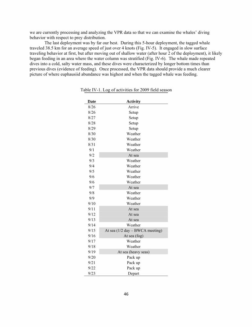
46 

 

we are currently processing and analyzing the VPR data so that we can examine the whales’ diving behavior with respect to prey distribution. The last deployment was by far our best. During this 5-hour deployment, the tagged whale traveled 38.5 km for an average speed of just over 4 knots (Fig. IV-5). It engaged in slow surface traveling behavior at first, but after moving out of shallow water (after hour 2 of the deployment), it likely began feeding in an area where the water column was stratified (Fig. IV-6). The whale made repeated dives into a cold, salty water mass, and these dives were characterized by longer bottom times than previous dives (evidence of feeding). Once processed, the VPR data should provide a much clearer picture of where euphausiid abundance was highest and when the tagged whale was feeding.

Table IV-1. Log of activities for 2009 field season

Date Activity 8/26 Arrive 8/26 Setup 8/27 Setup 8/28 Setup 8/29 Setup 8/30 Weather 8/30 Weather 8/31 Weather 9/1 Weather 9/2 At sea 9/3 Weather 9/4 Weather 9/5 Weather 9/6 Weather 9/6 Weather 9/7 At sea 9/8 Weather 9/9 Weather

9/10 Weather 9/11 At sea 9/12 At sea 9/13 At sea 9/14 Weather 9/15 At sea (1/2 day – BWCA meeting) 9/16 At sea (fog) 9/17 Weather 9/18 Weather 9/19 At sea (heavy seas) 9/20 Pack up 9/21 Pack up 9/22 Pack up 9/23 Depart

 

  

Figure IV-1. Tag and methods used to study bowhead whale foraging behavior during September 2009.

47 

 

 

Figure IV-2. Launched tag immediately prior to attaching to a bowhead.    

Figure IV-3. Two examples of bowhead diving behavior observed during tagging operations: feeding (top) and traveling (bottom).

48 

 

    

 

Figure IV-4. In-situ video plankton recorder images of euphausiids near a tagged bowhead whale.

Figure IV-5. Track of whale tagged in event #3. Locations of CTD/OPC/VPR casts shown as triangles, with the tagging location shown in green and the tag recovery location shown in red.

49 

 

Figure IV-6. Vertical structure of temperature and salinity in proximity to the bowhead whale tagged in event #3.

50 

 

51 

 

                                                           

SECTION V - NORTH SLOPE BOROUGH RESEARCH: EXAMINATIONS OF BOWHEAD STOMACH CONTENTS

AND LOCAL BOAT SURVEYS

J. Craig George and Gay Sheffield

North Slope Borough, Department of Wildlife Management and Alaska Department of Fish and Game

Background

Studies of the bowhead whale area at Barrow have been ongoing for four years beginning with the National Science Foundation’s (NSF) SNACs program in 20051. Examinations of bowhead stomach contents have been underway for over 30 years, beginning in the 1970s under NOAA-NMML and since 1981 by the North Slope Borough (NSB). The following report describes the North Slope Borough (NSB) Department of Wildlife Management’s and Alaska Department of Fish and Game (ADFG) activities with the BOWFEST study during 2008 and 2009. The NSB and ADFG work includes sampling stomachs of landed whales, boat-based surveys, project coordination, logistical assistance, and boat-based observations of feeding whales.

Objectives

1. Gather distribution data on bowhead whales in the study area (Barrow to Cape Simpson and offshore ~20 km) via local boat-based surveys before the official field sampling starts on ~15 August.

2. Document bowhead whale prey amounts and types in the stomachs of whales landed during the subsistence hunt of bowhead whales at Barrow and Kaktovik.

3. Document locations and basic behavior of feeding whales from a boat-based platform.

 1 SNACs began in 2004, but the first field season was 2005.

52 

 

LOCAL BOAT-BASED BOWHEAD WHALE SURVEYS

As in 2008, local whale hunters were hired to locate bowhead whales in the

BOWFEST study area, determine their behavior, assist with deploying acoustic oceanographic instruments, and other projects.

For 2009, we have records for 26 boat surveys. These surveys included opportunistic hunter observations and BOWFEST funded surveys which provided the bulk of the sightings. Survey data were available from 1 July to 16 September (Fig. V-1; Table V-1).

During the period from 1 July to 16 September, a total of 282 bowhead whales were seen plus an additional 34 unidentified whale sightings which may have been either bowhead or gray whales. Unlike last year, bowhead whales appeared to be more common than gray whales in the survey area, however not all gray whale sightings were recorded. As in 2008, most gray whales were seen west of the 156° W longitude line. Other species, incidental to the large whale surveys included: one harbor porpoise, numerous ringed, spotted, and bearded seals, and bird observations. No humpback or minke whales were recorded nor were swimming polar bears recorded in the survey area in 2009. It is possible that polar bears were seen in some surveys but not recorded as these are not target species. Walruses were reported as abundant on the 1 July survey by H. Brower but numbers were not recorded. Seals were generally ubiquitous through the area but not consistently recorded as they were not the survey’s target species.

Sea ice was mostly absent in the study area during August, all of September, and most of October.

Table V-1. Preliminary tally of whale, walrus and polar bear sightings during local boat surveys during fall 2008.

Species

2008 Totals

2009 Totals

Bowhead 48

282

Gray 54 81 Minke? 2 0 Polar Bear 4 0 Unidentified Whale 2 0 Walrus 2 02

Bowheads were almost continuously observed and reported by subsistence

hunters and also during boat surveys through summer 2009. On 1 July, nine bowheads were reported by Captain Harry Brower about 40 miles southwest of Barrow during an                                                             2 Walruses were seen in Chukchi waters, but numbers were not recorded during the 1 July survey by H. Brower.

53 

 

unrelated project. Most of these whales were very large and their behavior indicated they were feeding. On the evening of 24 July 2009, we observed 4- 5 bowheads in the Chukchi Sea (71° 17.476’ N; 156° 48.445’ W) only 0.5 km from the city of Barrow. These whales appeared to be feeding and had mud plumes associated with them. Local whalers found this unusual as did ourselves. Bowheads have not been observed feeding off Barrow during July. Also unusual was that the whales were fluke-up diving in only 5.5 to 6 m water depth (Fig. V-2). No anecdotal observations were made or whale surveys conducted again until 11 August.

On 11 August, three boats went out on formal BOWFEST surveys, and over 30 bowhead (including a cow/calf pair) and gray whales were observed from Point Barrow and east to Cape Simpson. Some exceptionally large bowheads were observed in deep waters NNE of Point Barrow by DWM personnel (Fig. V-1). Behaviors recorded were both feeding and migrating.

Following a period of bad weather that prevented any boat surveys from being conducted, crews went out again on 20 August, and several bowheads were seen. From 20 Aug through 11 September, when formal BOWFEST boat surveys ended, whales were regularly seen on every survey – with one exception. On 27 August, despite considerable effort by several boats, no bowheads were seen in the study area.

As in 2008, a few boat surveys were conducted in the nearshore Chukchi Sea SW of Barrow during 2009. Bowheads were seen on all surveys in 2009 unlike the boat survey results during 2008 (Fig. V-1).

Like last year, bowhead whales were concentrated east of Point Barrow and most were observed feeding. Water column, bottom (mud-plumes evident), and surface trawl feeding were observed. There was a paucity of sightings between Tapkaluk and Cooper Island, but densities increased again off east of Cooper Island. Also, many whales were seen by the Baumgartner tagging crew within the “box” noted in Figure V-1; however, they did not record individual whale locations. During tagging operations on 14 September, “dozens” of whales were observed north of Cooper Island, and 4 whales were successfully tagged with satellite transmitters. The previous day (13 September), BWASP surveys found record numbers of bowheads just a few miles east. Janet Clarke (pers. comm.) reported:

“On 13 October 2009, BWASP completed transects in Block 12, again under very good survey conditions. There were 25 sightings of 297 bowhead whales. Six of the sightings, of groups ranging from three to 186 whales, were recorded as feeding. Sediment was noted in the water, along with birds. Some surface feeding was noted (and photographed).” J. Clarke

The last survey was conducted on 16 September under poor visibility conditions

and 3 bowheads were seen (from MMS Vessel 1273). Our longstanding agreement with the Barrow Whaling Captain’s Association is to cease research operations at least one week prior to the fall hunt which began on 1 October.

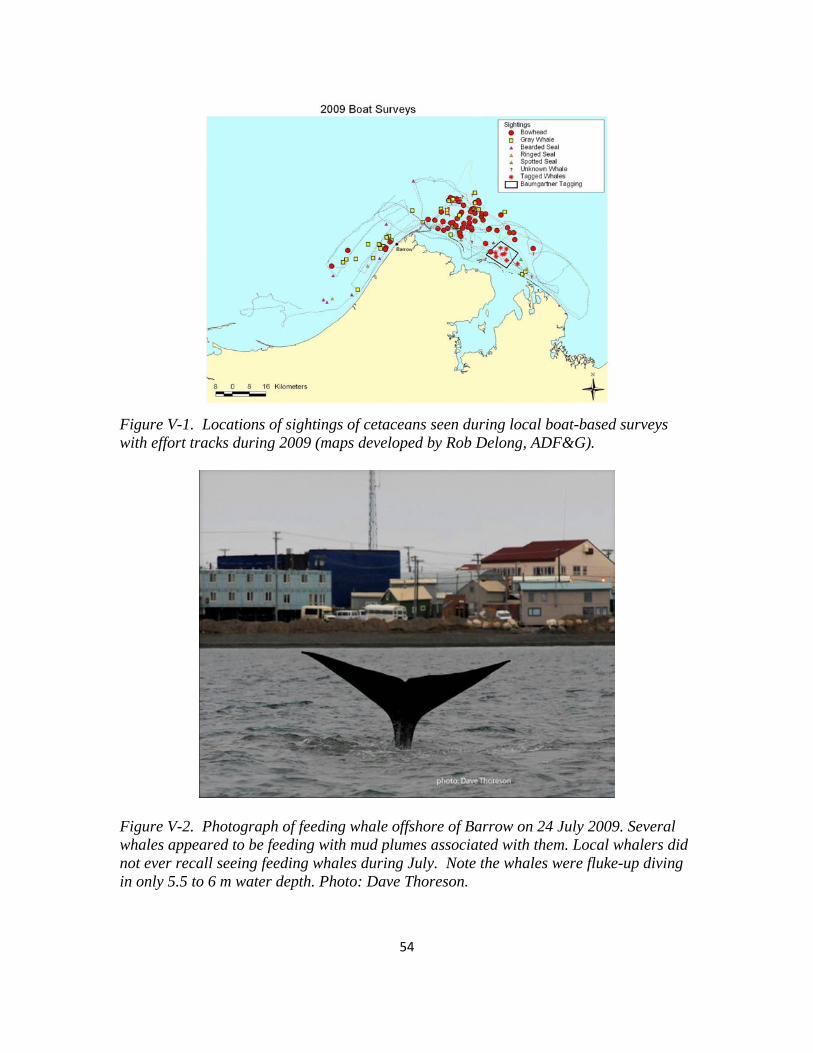
Figure V-1. Locations of sightings of cetaceans seen during local boat-based surveys with effort tracks during 2009 (maps developed by Rob Delong, ADF&G).

Figure V-2. Photograph of feeding whale offshore of Barrow on 24 July 2009. Several whales appeared to be feeding with mud plumes associated with them. Local whalers did not ever recall seeing feeding whales during July. Note the whales were fluke-up diving in only 5.5 to 6 m water depth. Photo: Dave Thoreson.

54 

 

55 

 

The 2009 surveys have again shown the utility of using local boat-based surveys and local knowledge to determine nearshore bowhead distribution and behavior, deploy small scientific instruments in nearshore Arctic waters, and conduct structure transects. Positive aspects of this methodology include: 1) local hunters are familiar with the region and distribution of marine mammals, 2) they understand the regional safety hazards and can operate safely, 3) they can refer to a large body of traditional knowledge to interpret their observations, 4) data from frequent hunting forays are available and valid, and 5) survey costs are modest compared with aircraft and large vessel charter.

Limitations include: 1) the use of small boats (< 9 m) which confines surveys to nearshore areas (< ~25 miles offshore), 2) space for scientific equipment is limited, and 3) personnel space is limited.

STOMACH EXAMINATIONS Results from 21 stomach samples from Barrow and Kaktovik 2008 harvests were

acquired. Of the nine whales examined during the 2008 Barrow spring harvest (April 27th – May 5th), 67% were not feeding, one whale contained a small sample of euphausiid fragments, and two were inconclusive (Table V-2). Interestingly, both harvested whales sampled (100%) during the 2008 spring harvest (7-27 April) near Saint Lawrence Island in the Bering Sea had been feeding recently on large calanoid copepods (Sheffield 2008).

During the 2008 fall harvest (5-23 October) near Barrow, 91% of the 11 whales examined had been feeding. Amphipods, euphausiids, mysids, and copepods were most frequently identified most frequently. Euphausiids dominated four of the five whales for which there was suitable prey volume data. By volume, copepods only dominated the sample of the last whale harvested (23 October). Of note, arctic cod (Boreogadus saida) were identified in 55% of the fall whales near Barrow. Appendix 1 provides a list of all taxa identified. Two of the three harvested whales harvested near Kaktovik during 2008 (6-13 Sept.) were feeding. Interestingly, 08KK1 had milk in the stomach but copepod remains were present in the feces indicating this 7.2 m whale was transitioning from nursing to feeding. This is the first observation we know of regarding the onset of feeding on solid foods in bowhead whales. Calanoid copepods dominated the stomach contents of 08KK3 with several mysids and amphipods present.

Bowhead whale stomachs and other tissues were collected during 2009 from the spring and fall whale hunt at Barrow and the fall hunt at Kaktovik (Table V-3). Preliminary analysis of 2009 Barrow bowhead stomachs indicated that during the spring harvest (17-23 May), one of two whales examined had been feeding and two were unexamined (Table V-4). As in 2008, samples from two whales harvested in the Bering Sea near Saint Lawrence Island during spring 2009 (15-18 April) had been feeding on large copepods, especially Calanus glacialis (Sheffield and George 2009).

Of the three harvested whales at Kaktovik during 2009, one stomach (09KK1) was cut during butchering but copepods and amphipods were identified in a duodenum sample, one whale stomach (09KK2) was distended with fresh euphausiid prey that included several invertebrate taxa and fish (Fig. V-3), and one stomach (09KK3) was empty.

During the 2009 fall harvest near Barrow (26 September – 10 October), 80% of

the 15 sampled whales were feeding, 1 had a trace of prey and 2 were inconclusive (watery fluid with no obvious prey). Stomachs of several fall whales were packed solid with fresh euphausiids (Fig. 4). This suggests that the krill were especially dense in 2009, the whales had been feeding at the time of death, or both.

The following manuscript describing the distribution, behavior, and information on local zooplankton occurrence as indicated by stomach contents from harvested whales in Barrow during 2005-2006 was accepted by the scientific journal Arctic:

Moore, S.E., J. C. George, G. Sheffield, J. Bacon, C. J. Ashjian. Late summer bowhead whale distribution and feeding in the western Alaskan Beaufort Sea, 2005-06. Arctic. (In Press – June 2010)

Table V-2. Status of bowheads harvested near Barrow and Kaktovik (Beaufort Sea) during 2008-2009, as well as Saint Lawrence Island (Bering Sea), and examined for evidence of feeding. Bering Sea -

spring Barrow -

spring Barrow –

fall Kaktovik - fall

2008

n=2

n=9

n=11

n=3

Feeding 100% 11% 91% 67% Not feeding 0% 67% 0% 33% Uncertain (trace)

0% 22% 9% 0%

2009 n=2 n=2 n=15 n=3 Feeding 100% 50% 80% 67% Not feeding 0% 50% 20% 33% Uncertain (trace)

0% 0% 0% 0%

56 

 

57 

 

Table V-3. Tissues collected from bowhead whales harvested near Kaktovik during September 2009 and showing the recipient of those tissues. 09KK1 09KK2 09KK3 Stomach contents ADF&G ADF&G - Feces ADF&G ADF&G ADF&G Blood NSB-DWM NSB-DWM NSB-DWM Urine - - NSB-DWM Blubber NSB-DWM NSB-DWM NSB-DWM Tongue NSB-DWM NSB-DWM NSB-DWM Kidney - NSB-DWM - Liver - NSB-DWM NSB-DWM Spleen NSB-DWM NSB-DWM NSB-DWM Muscle NSB-DWM NSB-DWM NSB-DWM Lung NSB-DWM NSB-DWM NSB-DWM Eyeball(s) NSB-DWM NSB-DWM NSB-DWM Intestine NSB-DWM NSB-DWM NSB-DWM Body fat NSB-DWM NSB-DWM NSB-DWM Heart - NSB-DWM - Skin NSB-DWM NSB-DWM NSB-DWM Baleen NSB-DWM NSB-DWM NSB-DWM Ovaries NSB-DWM - NSB-DWM Testes / Epididymis - NSB-DWM

-

Fetus NSB-DWM - - NSB-DWM = North Slope Borough, Department of Wildlife Management (Barrow) ADF&G = Alaska Dept. of Fish and Game (Nome)

58 

 

Table V-4. Basic data on bowhead whales harvested near Kaktovik and Barrow during 2009 with comments on feeding status.

ID # Location Date Sex Total length (m) Status 09KK1 Kaktovik Sep-09 F 15.3 Feeding 09KK2 Kaktovik Sep-09 M 13.2 Feeding 09KK3 Kaktovik Sep-09 F 6.6 Not feeding 09B1 Barrow May-09 F 8.4 Not feeding 09B2 Barrow May-09 M 14.8 Feeding 09B3 Barrow May-09 F 14.6 Not examined 09B4 Barrow May-09 - - Not examined 09B5 Barrow Sep-09 M 9.8 Feeding 09B6 Barrow Sep-09 M 9.9 Feeding 09B7 Barrow Sep-09 F 11.3 Feeding 09B8 Barrow Sep-09 F 10.3 Feeding 09B9 Barrow Sep-09 M 8.7 Feeding 09B10 Barrow Sep-09 F 8.9 Feeding 09B11 Barrow Sep-09 F 7.2 Sample pending 09B12 Barrow Sep-09 F 8.7 Uncertain (trace) 09B13 Barrow Sep-09 M 8.1 Uncertain (trace) 09B14 Barrow Sep-09 F 10.2 Feeding 09B15 Barrow Oct-09 M 8.7 Feeding 09B16 Barrow Oct-09 F 7.8 Feeding 09B17 Barrow Oct-09 F 9.9 Feeding 09B18 Barrow Oct-09 M 8.4 Feeding 09B19 Barrow Oct-09 F 10.6 Feeding

59 

 

Appendix V-1. Prey items consumed by bowhead whales harvested in the Alaskan Beaufort Sea, 2008.

Copepods Decapods

Calanus glacialis Eualus gaimardi Calanus hyperboreus Hippolytidae Metridea longa Sabinea septemcarinata Paeuchaeta sp. Paguridae zoea Paeuchaeta glacialis Fish Mysids Boreogadus saidaMysis sp. Mysis occulata Neomysis rayii Cumacea Diastylis sp. Isopods Saduria entomon Amphipods Acanthostepheia behringiensisAmpelisca sp. Anonyx sp. Onissimus sp. Pontoporeia sp. Pontoporeia femorataHyperiid amphipodsGammarid amphipods Euphausiids Thysanoessa sp. Thysanoessa inermis Thysanoessa raschii

Figure V-3. Photo of stomach from whale 09KK2, this stomach was distended with fresh euphausiid prey (spilling out on right) that also included several invertebrate taxa and fishes.

Figure V-4. Photo of stomach from whale 09B8. This stomach was also distended with fresh euphausiid prey and little else. The prey was densely packed with little stomach fluid, which is uncommon.

60 

 

BOWFEST 2009 REPORT 

Literature Cited

Sheffield, G. 2008. Bowhead Whale Diet Investigation: St. Lawrence Island, Bering Sea. Final Federal Aid Report. Grant T1, Project No. 3. 12. 12 pp.

Sheffield, G. and J. C. George. 2009. Bowhead whale feeding in the northern Bering Sea near

Saint Lawrence Island, Alaska. SMM Biennial Conference on the Biology of Marine Mammals, 12-16 October 2009. Abstract. 

61 

 

BOWFEST 2009 REPORT 

BOWFEST PRESENTATIONS AND MEETINGS IN 2009

2009 Jan 20: BOWFEST Workshop, Anchorage. Logistics and results of the 2008 field season were discussed, and plans for 2009 were formulated; 32 attendees.

2009 Jan 20-23: Alaska Marine Science Symposium, Anchorage. The following presentations

were based, at least in part, on BOWFEST research:

Koski, W., D. Rugh, J. Mocklin, K. Goetz, K. Trask, and J.C. George. Calibration of bowhead whale measurements from photographs using over-land and over-water calibration targets. Poster.

Goetz, K., D. Rugh, and J. Mocklin. Bowhead Whale Feeding Ecology Study

(BOWFEST) Aerial Surveys: A comparison of bowhead whale distribution and survey effort in 2007and 2008 in the vicinity of Barrow, Alaska. Poster.

Okkonen, S., C. Ashjian, and R. Campbell. Upwelling and aggregation of zooplankton on

the western Beaufort shelf as inferred from moored acoustic Doppler current profiler measurements . Poster.

2009 Jan 29: Barrow Whaling Captain’s Association meeting; C. George, C. Ashjian, and M.

Baumgartner present updates on BOWFEST activity. 2009 Apr 13: NMML seminar. Mocklin. Evidence of feeding by bowhead whales from aerial

photography. 2009 Apr 20: Univ. of Washington Wildlife Seminar Series. Mocklin., Evidence of feeding by

bowhead whales from aerial photography. 2009 May 2: Northwest Student Chapter of Marine Mammalogy (Western Washington Univ.,

Vancouver). Mocklin. Evidence of feeding by bowhead whales from aerial photography. 2009 May18-22: Acoustical Society of America, 157th Meeting, Portland, Oregon:

Stafford, K., S. Moore, C. Berchok, and D. Mellinger. Acoustic sampling for marine mammals in the Beaufort Sea July 2007-March 2008. Invited paper.

Heimlich, S.M., D.K. Mellinger, S.L. Nieukirk, H. Klinck, K.M. Stafford, S.E. Moore,

and P.J. Stabeno. Detecting bowhead whale sounds in the Beaufort Sea: Confounding sounds in a cacophony of noise.

2009 June 24: NMML seminar. Rugh. NMML’s Arctic Whale Research. 2009 Aug 20: Meeting in Barrow at the start of the 2009 BOWFEST season. Ashjian, Campbell,

Okkonen, Alatalo, George, Rugh, DeMaster, Clarke, Ferguson.

62 

 

BOWFEST 2009 REPORT 

63 

 

2009 Sept 6: BOWFEST dinner meeting in Barrow with 23 researchers and support crew. 2009 Sept 9: BOWFEST meeting in Barrow with 20 researchers attending. 2009 Oct: Biennial Marine Mammal Conference in Quebec City, Canada:

Ferguson, M., R. Angliss, D. Rugh, J. Mocklin, and L. Vate Brattström. Comparison of unmanned aircraft systems (UASs) and manned aircraft for surveying bowhead whale distribution and density. Workshop presentation.

Mocklin, J. , Rugh, D. , and Moore, S. Evidence of feeding by bowhead whales from

aerial photography. Poster. Heimlich, S.M., D.K. Mellinger, H. Klinck, K.M. Stafford, S.E. Moore, C.L. Berchok,

and S.L. Nieukirk. Detecting bowhead whale sounds in the Beaufort Sea: Confounding sounds in a cacophony of noise.

2009 Dec: Rugh, D. and J. Mocklin. Aerial Surveys to Study Bowhead Whale Feeding Ecology.

Quarterly Reports for the Alaska Fisheries Science Center, NOAA Fisheries Service.

2010 Jan 19-22: Alaska Marine Science Symposium, Anchorage. The following presentations

were based, at least in part, on BOWFEST research:

Stafford, K.M., C. L. Berchok, D.K. Mellinger, and S.E. Moore. Ambient noise in the Alaskan Beaufort Sea 2007-2009. Poster.

Baumgartner, M.F. and T.R. Hmmar. Using a new short‐term dermal attachment tag to

study bowhead whale foraging ecology in the western Beaufort Sea. Poster. Ashjian, C.J., R.G. Campbell, S.R. Okkonen, B.F. Sherr, and E.B. Sherr. Year‐to‐year

variability of ocean biology at a bowhead whale feeding hotspot near Barrow, AK: 2005‐2009. Poster.

Rugh, D., C. Ashjian, M. Baumgartner, C. Berchok, R. Campbell, J.C. George, K. Goetz,

D. Mellinger, J. Mocklin, S. Okkonen, G. Sheffield, M. Smultea, and K. Stafford. The Bowhead Whale Feeding Ecology Study (BOWFEST). Poster.

Mocklin, J., D. Rugh, and S. Moore. Using aerial photography to investigate evidence of

feeding by bowhead whales. Oral presentation. Smultea, M., D. Rugh, and D. Fertl. Review of systematic surveys involving bowhead

whales in the U.S. Beaufort and Chukchi seas 1975 – 2009. Poster. Okkonen, S., C. Ashjian, and B. Campbell. Multi-platform observations of circulation

features associated with the Barrow area Bowhead whale feeding hotspot. Poster