www.oeaw.ac.at

www.ricam.oeaw.ac.at

Boundary-element-basedfinite element methods forHelmholtz and Maxwellequations on generalpolyhedral meshes

D. Copeland

RICAM-Report 2008-11

BOUNDARY-ELEMENT-BASED FINITE ELEMENT METHODS FOR

HELMHOLTZ AND MAXWELL EQUATIONS ON GENERAL

POLYHEDRAL MESHES

DYLAN M. COPELAND∗

Abstract. We present new finite element methods for Helmholtz and Maxwell equations for gen-eral three-dimensional polyhedral meshes, based on domain decomposition with boundary elementson the surfaces of the polyhedral volume elements. The methods use the lowest-order polynomialspaces and produce sparse, symmetric linear systems despite the use of boundary elements. Moreover,piecewise constant coefficients are admissible. The resulting approximation on the element surfacescan be extended throughout the domain via representation formulas. Numerical experiments confirmthat the convergence behavior on tetrahedral meshes is comparable to that of standard finite elementmethods, and equally good performance is attained on more general meshes.

1. Introduction. In industrial applications involving the numerical solution ofpartial differential equations, refinement of a given mesh may be infeasible due to aprohibitively large number of degrees of freedom. If the mesh consists of elementsbeyond the simplest types commonly used (e.g. tetrahedra, hexahedra, prisms), thenstandard finite element methods cannot be applied without refinement. Even if finiteelement methods are known for the various types of elements in a mesh, the imple-mentation and solution via finite element methods can be quite difficult and expensivefor meshes with many different types of elements. Thus there is a need for numericalmethods which can be applied robustly to any polyhedral mesh, without refinementor special treatment of each of the various element types. We propose such a methodfor the Helmholtz and Maxwell equations, including the Laplace equation as a specialcase (with wavenumber equal to zero).

The mimetic finite difference (MFD) method has been proposed for numericallysolving partial differential equations on general polygonal or polyhedral meshes. TheMFD method has been proven effective for diffusion problems (see e.g. [3, 23, 24]),and in [22], an MFD method for Maxwell equations in two dimensions is presented,which could be extended to three dimensions. However, this method relies on alogically rectangular mesh structure, and there seems to be no MFD method forMaxwell equations on general meshes.

The discontinuous Galerkin (DG) method appears to be a more promising ap-proach for discretization on general meshes. DG methods are known to treat general,non-conforming meshes with ease, and methods for Maxwell equations have beenwell studied– see e.g. [14, 19, 20] and the references therein. However, the authoris unaware of any study of DG methods for Maxwell equations applied to generalthree-dimensional meshes.

In this paper, we propose a new discretization method based on boundary integraltechniques. Boundary element methods have been widely studied and have provenvery effective in many types of problems with constant coefficients. Boundary integralrepresentation formulas give the solution in a domain as an expression involving onlyits traces on the boundary, thereby reducing the problem to the boundary. Thisdimension reduction makes boundary element methods much faster and more efficientthan finite element methods in some cases. However, boundary element methods havesome drawbacks in general, such as the limited applicability to problems with constant

∗Johann Radon Institute for Computational and Applied Mathematics, Austrian Academy ofSciences, Altenbergerstrasse 69, A-4040 Linz, Austria. E-mail: dylan.copeland@ricam.oeaw.ac.at.

1

2 D.M. COPELAND

coefficients and the practical necessity of data-sparse approximations of the denselinear systems that result from discretization. As a result, some very efficient methodshave been designed by coupling boundary element and finite element methods indifferent subdomains as appropriate. For example, in [17, 18], scattering problems areefficiently solved by coupling boundary elements in the unbounded exterior domain,where the coefficient is constant, with finite elements in the interior domain, wherethe coefficient may vary. In principle, we take a similar approach for acoustic andelectromagnetic scattering problems, but in this paper we focus only on developingfinite-element-type discretizations for the bounded interior domain. It is a simplematter to couple our method with a boundary element method in the exterior domain,and we will indicate how this can be done.

Given a general polyhedral mesh of the bounded domain, we follow the domaindecomposition approach of [21] and apply boundary integral techniques on the sur-faces of the polyhedral elements. That is, we treat the elements as subdomains anddiscretize the element surfaces with boundary element spaces. Strictly speaking, theresulting method is a boundary element domain decomposition, but we refer to itas a boundary-element-based finite element method due to its similarity to finite ele-ment methods with respect to several fundamental properties. For instance, piecewiseconstant coefficients are admissible, and the resulting linear system is sparse, withcoupling only between degrees of freedom in the same volume element.

The methods developed in this paper can also be viewed strictly as domain de-composition methods analogous to [21], for subdomains of any size. Such methodswere studied in [21] for scalar elliptic partial differential equations, but we extendthose results to the Helmholtz and Maxwell equations. In particular, we analyze theDirichlet-to-Neumann maps and prove that they satisfy generalized Garding inequal-ities. Thus the present paper is of both a finite element and domain decompositionnature, depending on one’s interpretation. In the theoretical analysis, we can onlyprove error estimates for a pure domain decomposition setting, with subdomains offixed size. However, the numerical experiments reported in this paper investigatethe method in a finite element setting, demonstrating error behavior comparable tooptimal finite element methods.

For a practical implementation, we require a triangular mesh of the skeleton com-prised of the element surfaces. Alternatively, one could just as easily use a quadri-lateral skeleton mesh. Note that hanging nodes are inadmissible, as the method usesa conforming finite dimensional subspace of a trace space on the skeleton. Thus ourmethod allows for general volume elements but requires a triangular or quadrilateralmesh of the skeleton. As standard finite element methods can be applied only afterrefinement of the volume elements to geometrically simple elements, for some meshesour method involves significantly fewer degrees of freedom than standard finite ele-ment methods despite the necessary refinement of the mesh skeleton to triangular orquadrilateral surface elements.

The paper is organized as follows. In section 2, we define some trace operators andrelevant Sobolev spaces on the boundary of a Lipschitz polyhedral domain. Sections3 and 4 have very similar structure, as they describe the boundary-element-basedfinite element method applied to the Helmholtz and Maxwell equations, respectively.Finally, we report on some numerical experiments in section 5.

2. Preliminaries. The methods proposed in this paper solve for traces of solu-tions to the Helmholtz or Maxwell equations and therefore require some theory forthe trace operators and the Sobolev spaces onto which they map. In this section, we

BOUNDARY-ELEMENT-BASED FINITE ELEMENT METHODS 3

briefly present the necessary theory for Lipschitz polyhedral domains.On a Lipschitz polyhedral domain Ω and its boundary Γ := ∂Ω, the complex-

valued Sobolev spaces Hs(Ω) and Ht(Γ) are defined for all s in R and |t| ≤ 1 [1, 25],with L2 := H0. The inner product < ·, · >Γ in L2(Γ) is defined by

< u, v >Γ:=

∫

Γ

uv dS for all u, v in L2(Γ).

The inner product (·, ·)Ω in L2(Ω) is defined analogously. To formulate a method forsolving the Helmholtz equation, we shall utilize the standard Dirichlet and Neumanntrace operators γ0 : H1

loc(R3) → H

1

2 (Γ) and γ1 : Hloc(∆,R3\Γ) → H− 1

2 (Γ) (cf. [13]),where

Hloc(∆,R3 \ Γ) := φ ∈ H1

loc(R3 \ Γ) : ∆φ ∈ L2

loc(R3 \ Γ).

The polyhedral boundary Γ can be decomposed as a union Γ = ∪NΓ

j=1F j of openplanar polygonal faces Fj , 1 ≤ j ≤ NΓ. Let n denote the unit outward normal vectorto Ω, and set nj := n|Fj . Further, let eij denote the open edge between the faces Fi

and Fj , i.e. eij = F i ∩ F j , and τij an arbitrary unit vector parallel to the edge eij .Then τi, τij, with τi := τij × ni, is a basis of the plane containing Fi.

Next, we define the appropriate function spaces for the tangential traces involvedin solving Maxwell’s equations. Theory for these spaces was developed in [5, 6], andwe follow the notation therein. First, define the spaces

L2t(Γ) := v ∈ L2(Γ)3 : v · n = 0 on Γ,

H1/2− (Γ) := v ∈ L2

t(Γ) : vj ∈ H1/2(Fj), 1 ≤ j ≤ NΓ,

and define the tangential components trace mapping πτ : D(Ω)3 → H1/2− (Γ) and the

tangential trace mapping γt : D(Ω)3 → H1/2− (Γ) by πτ (v) := n × (v × n)|Γ and

γt(v) := v×n|Γ. The tangential components trace πτ (v) of a vector field v in H1(Ω)is clearly in H1/2(Fj) for each face Fj , and it was shown in [5] that πτ (v) is weakly

tangentially continuous across each edge eij . To be precise, the functional N‖ij defined

by

N‖ij(φ) :=

∫

Fi

∫

Fj

|φi · τij(x) − φj · τij(y)|2

‖x − y‖3dSx dSy

is finite when applied to πτ (v). By [5, Proposition 2.6],

(2.1) H1/2‖ (Γ) := v ∈ H

1/2− (Γ) : N

‖ij(v) <∞ for all edges eij

is a Hilbert space with the norm

‖v‖2‖,1/2,Γ :=

NΓ∑

j=1

‖v‖21/2,Γj

+∑

eij

N‖ij(v).

Moreover, πτ : H1(Ω) → H1/2‖ (Γ) is linear, continuous, and surjective [5, Proposition

2.7]. We denote by H−1/2‖ (Γ) the dual space of H

1/2‖ (Γ), with L2

t(Γ) as the pivot

4 D.M. COPELAND

space, and by < ·, · >‖,1/2,Γ the duality pairing between H−1/2‖ (Γ) and H

1/2‖ (Γ). The

tangential traces of vector fields in H(curl,Ω) are contained in the space

H−1/2‖ (divΓ,Γ) := v ∈ H

−1/2‖ (Γ) : divΓ(v) ∈ H−1/2(Γ),

where divΓ : H−1/2‖ (Γ) → H−3/2(Γ) is the surface divergence operator defined in [5].

By [5, Theorem 3.9], γt : H(curl,Ω) → H−1/2‖ (divΓ,Γ) is linear and continuous. In

solving the Maxwell equations, H−1/2‖ (divΓ,Γ) will be the appropriate function space

for the tangential traces.

As this paper is concerned with complex-valued Helmholtz and Maxwell systems,the associated bilinear forms are not elliptic. Therefore, we must consider a general-ized notion of coercivity suitable for our purposes.

Definition 1. A bilinear form a : X ×X → C on a reflexive Banach space X issaid to be coercive if it satisfies a generalized Garding inequality of the form

Re (a(u,Θu)− c(u, u)) ≥ C‖u‖2X for all u ∈ X,

where C > 0, c : X × X → C is a compact bilinear form, and Θ : X → X is anisomorphism.

A continuous bilinear form a : X × X → C induces a bounded linear operatorA : X → X ′ (where X ′ denotes the dual space), defined by

< Av,w >:= a(v, w) for all v, w in X.

If the bilinear form a(·, ·) is coercive, then the associated operator A is Fredholmwith zero index (see e.g. [25]). Therefore, injectivity implies invertibility (see [7,Proposition 3], [27, Theorem 3.15]). Thus we have the following abstract result,whereby we prove the unique solvability of all variational problems considered in thispaper.

Lemma 1. If a bilinear form a : X × X → C is coercive and the associatedoperator A : X → X ′ is injective, then the inverse A−1 : X ′ → X exists and iscontinuous.

3. The Helmholtz Equation. Consider the Helmholtz equation for acousticscattering, which involves both an interior and exterior domain. Accordingly, letΩ− := Ω ⊂ R

3 be a bounded Lipschitz polyhedral domain, and denote by Ω+ :=

R3 \ Ω−

its open complement. Often, we simply write Ω instead of Ω−. The unitnormal vector n on Γ := ∂Ω− is defined as pointing from Ω− into Ω+. For any traceoperator γ, γ+ and γ− denote the traces from Ω+ and Ω−, respectively. For example,γ±1 φ = (∇φ|Ω±) · n for φ in D(R3), with the same normal n in both cases. The jumpin a trace operator γ is denoted by [γφ]Γ = γ+φ− γ−φ. With this notation, we statethe Helmholtz equation with transmission and radiation conditions as

(3.1)

∆u+ κ2u = 0 in Ω− ∪ Ω+,γ+0 u

s − γ−0 u = −γ+0 u

i on Γ := ∂Ω−,∂u∂r (x) − iκu(x) = o(r−1) uniformly for r := |x| → ∞.

Here, ui and us denote the incident and scattered waves, respectively. In the exteriordomain Ω+, u = ui + us.

BOUNDARY-ELEMENT-BASED FINITE ELEMENT METHODS 5

For simplicity, in this paper we present a method for solving the interior Dirichletproblem

(3.2)

∆u+ κ2u = 0 in Ω−,γ−0 u = g on Γ,

for some function g in H1/2(Γ). The method can easily be extended to solve (3.1), aswe shall indicate in a remark. We assume that κ > 0 is constant in Ω+ and piecewiseconstant in Ω− and that the differential operator ∆ + κ2I : H(∆,Ω−) → L2(Ω−)has a trivial null space. In the case that κ is constant in Ω−, this means that κ2 isbounded away from the interior Dirichlet eigenvalues of −∆ in Ω−.

3.1. Boundary Integral Operators. In this section, we define the necessaryboundary integral operators on a general Lipschitz polyhedral domain Ω with bound-ary Γ and a constant wavenumber κ > 0. The theory for this section is quite technicaland has already been established in the literature, so we only give a survey here ofthe results necessary for our purposes. For further details, see e.g. [11, 18].

The key to the boundary integral approach is the representation formula (cf. [25,Theorem 6.10])

(3.3) u(x) = −

∫

Γ

Eκ(x − y) [γ1u]Γ dSy +

∫

Γ

∂Eκ(x − y)

∂n(y)[γ0u]Γ dSy,

for x in Ω− ∪ Ω+, where

Eκ(x) =eiκ|x|

4π|x|for x 6= 0,

is the fundamental solution of the Helmholtz equation with the constant wavenumberκ > 0. The representation formula (3.3) yields a solution to (3.1) in terms of theDirichlet and Neumann traces, provided that the wavenumber κ is constant. Definingthe scalar single-layer and double-layer potentials

ψSLκ : H− 1

2 (Γ) → H1loc(R

3) ∩Hloc(∆,R3 \ Γ),

ψDLκ : H

1

2 (Γ) → Hloc(∆,R3 \ Γ),

(see [25, Theorem 6.12]) by

ψSLκ φ(x) :=

∫

Γ

Eκ(x − y)φ(y) dSy , x in Ω− ∪ Ω+,

ψDLκ φ(x) :=

∫

Γ

∂Eκ(x − y)

∂n(y)φ(y) dSy, x in Ω− ∪ Ω+,

we may rewrite the representation formula (3.3) as

(3.4) u = −ψSLκ ([γ1u]Γ) + ψDL

κ ([γ0u]Γ) in Ω− ∪ Ω+.

In this paper, we solve the interior Dirichlet problem (3.2) and therefore employ therepresentation formula

(3.5) u = ψSLκ

(

γ−1 u)

− ψDLκ

(

γ−0 u)

in Ω−,

6 D.M. COPELAND

given in terms of the interior traces only. As in [11, 18, 25], the trace operators γ±0and γ±1 may be applied to (3.5), yielding the the exterior (with the superscript +)and interior (with the superscript −) Calderon projectors

(3.6) P±H =

[

12I ±K ∓V∓D 1

2I ∓K ′

]

: H1/2(Γ) ×H−1/2(Γ) → H1/2(Γ) ×H−1/2(Γ),

where

V : Hs(Γ) → Hs+1(Γ), − 1 ≤ s ≤ 0, V := γ0ψSLκ Γ,

K : Hs(Γ) → Hs(Γ), 0 ≤ s ≤ 1, K := γ0ψDLκ Γ,

K ′ : Hs(Γ) → Hs(Γ), − 1 ≤ s ≤ 0, K ′ := γ1ψSLκ Γ,

D : Hs(Γ) → Hs−1(Γ), 0 ≤ s ≤ 1, D := −γ1ψDLκ Γ,

are continuous boundary integral operators (cf. [11, 25]). Here, Γ denotes theaverage across Γ, e.g. γ0φΓ = 1

2 (γ+0 φ+ γ0φ

−).

If u is a solution to (3.1), then the pair of traces (γ±0 u, γ±1 u) is referred to as

exterior/interior Cauchy data. The space of all interior Cauchy data for the Helmholtzequation coincides with the range of P−

H . As a consequence of this fact, the interiorNeumann trace of a Helmholtz solution can be expressed in terms of the interiorDirichlet trace via the operator

(3.7) S− : H1

2 (Γ) → H− 1

2 (Γ), S− := D + (1

2I +K ′)V −1(

1

2I +K),

which is referred to as the interior Dirichlet-to-Neumann map. The existence of theinverse V −1 is given next in Proposition 1.

Lemma 2. The boundary integral equation

(3.8) V η = (1

2I +K)ξ, with (ξ, η) in H1/2(Γ) ×H−1/2(Γ),

holds if and only if (ξ, η) are interior Cauchy data for a Helmholtz solution.

Proof. If (ξ, η) are interior Cauchy data, then (3.8) is the first row of P−H (ξ, η) =

(ξ, η). Conversely, if (3.8) holds, then the first component of P+H (ξ, η) is zero. Since

P+H (ξ, η) is in the range of P+

H , it is exterior Cauchy data with vanishing Dirichlettrace. It follows from the uniqueness of solutions to the exterior Dirichlet problem[25, Theorem 9.10] that P+

H (ξ, η) = 0. Thus (ξ, η) are interior Cauchy data.

Proposition 1. The operator V : H− 1

2 (Γ) → H1

2 (Γ) has a bounded inverse

V −1 : H1

2 (Γ) → H− 1

2 (Γ).

Proof. By [13, Theorem 2], V is coercive and hence Fredholm of index zero. Toverify the injectivity of V , suppose that V η = 0. By Lemma 2, (0, η) are interiorCauchy data. Under the assumption that κ2 is not an interior Dirichlet eigenvalue of−∆, we have that η = γ−1 0 = 0, which proves the injectivity of V . Therefore, V hasa bounded inverse.

For x in Γ and sufficiently smooth φ, we have the following expressions for theaction of the aforementioned boundary integral operators:

V φ(x) =∫

ΓEκ(x − y)φ(y) dSy , Kφ(x) =∫

Γ∂Eκ(x−y)

∂n(y) φ(y) dSy ,

K ′φ(x) =∫

Γ∂Eκ(x−y)

∂n(x) φ(y) dSy , Dφ(x) = − ∂∂n(x)

∫

Γ∂Eκ(x−y)

∂n(y) φ(y) dSy.

BOUNDARY-ELEMENT-BASED FINITE ELEMENT METHODS 7

3.2. Element-wise Domain Decomposition. Given a mesh of the boundeddomain Ω−, we propose a domain decomposition method based on [21] to solve forthe Dirichlet trace of the solution to (3.2) on the skeleton of the mesh. Locally onthe surface of each volume element, one can then obtain the Neumann trace from theDirichlet trace by applying the local Dirichlet-to-Neumann map. The solution insidethe volume element is then given by the representation formula (3.3).

Consider a general conforming polyhedral mesh of the bounded domain Ω− as adomain decomposition:

Ω−

= ∪pi=1Ωi, Ωi ∩ Ωj = ∅ for i 6= j,

where each Ωi is a simply-connected Lipschitz polyhedron. Conformity means thatfor i 6= j, Ωi ∩Ωj is empty, a vertex, an edge, or a polygonal face. The case of interestis diam(Ωi) ≈ h, but for theoretical analysis we only consider the simple case thatthe subdomains Ωi are of fixed size, with a family of meshes defined on their surfaces.In order to use boundary integral equations, we require that the mesh resolve anydiscontinuities in the wavenumber κ; i.e. κi := κ|Ωi is constant on Ωi, for each i.Denote the local boundaries by Γi = ∂Ωi and the mesh skeleton by ΓS = ∪p

i=1Γi.

Then H1

2 (ΓS) denotes the space of traces of functions in H1(Ω) on ΓS , and

‖φ‖H1/2(ΓS) :=

p∑

j=1

‖φ|Γj‖2H1/2(Γj)

1/2

defines a norm. We shall apply the results stated in the previous section for thedomains Ωi. Throughout the remainder of the paper, C represents a generic constantindependent of h but possibly depending on the wavenumber κ.

Let g be an arbitrary extension of g in H1(Ω), and set g := γS0 g, where γS

0 denotesthe trace on ΓS . Since the Dirichlet trace on Γ is given as data g, we need only solvefor the Dirichlet trace on ΓS \ Γ. Accordingly, we define the test function space

W := v ∈ H1/2(ΓS) : v = 0 on Γ

and seek u in W such that u+ g is the trace of u on ΓS . Then we have the followingvariational problem for u:

(3.9)

Find u ∈W such that u = u+ g on ΓS andaH(u, v) = −aH(g, v) for all v ∈W,

where the bilinear form aH : W ×W → C is defined by

(3.10) aH(v, w) =

p∑

i=1

< S−i vi, wi >Γi .

Here and throughout the remainder of the paper, φi denotes the restriction of a scalaror vector-valued function φ to Γi. Each operator S−

i is defined by (3.7), with theboundary integral operators Vi, Ki, and Di defined on the subdomain Ωi.

Remark 1. The existence of V −1i is given by Proposition 1, provided that κi is

not an interior Dirichlet eigenvalue of −∆ on Ωi. In the case that diam(Ωi) ≈ hfor sufficiently small h, a simple scaling argument shows that this condition holds.Indeed, the eigenvalues of −∆ on Ωi equal h−2 times the eigenvalues λj(Ωi) of −∆

8 D.M. COPELAND

on H10 (Ωi), where Ωi := h−1(x−xi,c) : x ∈ Ωi and xi,c is the center of mass of Ωi.

For κ2i < h−2λmin(Ωi), −∆−κ2

i I is positive definite on H10 (Ωi), and Vi has a bounded

inverse. In practice, the condition h < Cκ−1i is not restrictive, as it is necessary for

accurate approximation of the solution.Remark 2. The scattering problem (3.1) in R

3 can be solved by including the term< S+vΓ, wΓ >Γ in the sum (3.10), where S+ is the exterior Dirichlet-to-Neumannmap defined on H1/2(Γ). Analogous to S−, an expression for S+ can be derived fromthe fact that the range of P+

H is the space of all exterior Cauchy data. The space Wshould then be H1/2(ΓS).

Lemma 3. For each 1 ≤ i ≤ p, the local operator S−i is coercive. More precisely,

there exists a compact bilinear form ci : H1

2 (Γi) ×H1

2 (Γi) → C such that

(3.11) Re(

< S−i u, u >Γi −ci(u, u)

)

≥ C‖u‖2

H1

2 (Γi)for all u ∈ H

1

2 (Γi).

Proof. By [18, Lemma 3.2] (see also [11, 25]), the boundary integral operators

Di : H1

2 (Γi) → H− 1

2 (Γi) and Vi : H− 1

2 (Γi) → H1

2 (Γi) are coercive; specifically, there

exist compact operators TDi : H1

2 (Γi) → H− 1

2 (Γi) and TVi : H− 1

2 (Γi) → H1

2 (Γi)such that

Re < ξ, (Vi + TVi)ξ >Γi ≥ C‖ξ‖2

H− 1

2 (Γi), for all ξ in H− 1

2 (Γi),

Re < (Di + TDi)φ, φ >Γi ≥ C‖φ‖2

H1

2 (Γi), for all φ in H

1

2 (Γi).

Moreover, [18, Lemma 3.3] states that K ′i equals the L2(Γi)-adjoint K∗

i of Ki plusa compact perturbation, i.e. there exists a compact operator TKi : H−1/2(Γi) →H−1/2(Γi) such that

< (K ′i + TKi)ξ, φ >Γi=< K∗

i ξ, φ >Γi .

Denoting TKi := TKiV−1i (1

2I +Ki), we have

Re <(S−i + TDi + TKiφ, φ >Γi

= Re < (Di + TDi)φ, φ >Γi +Re < (1

2I +K ′

i + TKi)V−1i (

1

2I +Ki)φ, φ >Γi

≥ C‖φ‖2

H1

2 (Γi)+ Re < (

1

2I +K∗

i )V −1i (

1

2I +Ki)φ, φ >Γi

= C‖φ‖2

H1

2 (Γi)+ Re < V −1

i (1

2I +Ki)φ, ViV

−1i (

1

2I +Ki)φ >Γi

and hence

Re

(

< (S−i + TDi + TKi)φ, φ >Γi + < V −1

i (1

2I +Ki)φ, TViV

−1i (

1

2I +Ki)φ >Γi

)

≥ C‖φ‖2

H1

2 (Γi),

which verifies (3.11). Thus we have proved the coercivity of S−i .

Theorem 1. The variational problem (3.9) has a unique solution in W .Proof. We need only verify the hypotheses of Lemma 1. The coercivity of aH :

W ×W → C follows immediately from the local coercivity result stated in Lemma 3.

BOUNDARY-ELEMENT-BASED FINITE ELEMENT METHODS 9

To verify the injectivity of the operator A, suppose that Av = 0 for some v in W . Foreach 1 ≤ i ≤ p, vi := v|Γi is in H1/2(Γi), and (vi, S

−i vi) are Cauchy data for some

local function φi in H1(Ωi) satisfying

∆φi + κ2φi = 0 in Ωi,γ−0 φi = vi on Γi,γ−1 φi = S−

i vi on Γi.

For all w in W , we have

p∑

i=1

< γ−1,iφi, wi >Γi=

p∑

i=1

< S−i vi, wi >Γi= aH(v, w) =< Av,w >= 0.

Hence the global function φ, defined by φ = φi on Ωi, is in H1(Ω−) and satisfies theinterior Dirichlet problem

∆φ+ κ2φ = 0 in Ω−,γ−0 φ = 0 on Γ.

Under the assumption that ∆+κ2I has a trivial null space, we have φ = 0 and hencev = 0. This shows that A is injective and completes the proof of the theorem.

As mentioned in the introduction, the method (3.9) can be considered as eithera finite element method or a domain decomposition method, depending on the choiceof the subdomains Ωj . If one takes the subdomains to be volume elements of size h,then a finite element method is obtained. In this case, the wavenumber may be equalon different subdomains. Alternatively, one may take the subdomains to be maximalwith respect to the constant values of the wavenumber. The resulting pure boundaryelement domain decomposition method would require fewer degrees of freedom, asthe skeleton mesh would be significantly smaller. The disadvantage in this would bethe large dense matrices on each subdomain, necessitating sophisticated techniquesfor efficient data-sparse approximation of dense boundary element matrices (see, e.g.[2, 16, 27]). Additionally, the inversion of the single layer potential operator V in theapplication of the Dirichlet-to-Neumann maps would become expensive. One mayindeed find the necessary tools to make this approach feasible in practice, but in ournumerical computations we take the “finite element” approach with element-sizedsubdomains.

3.3. Discretization. We now discretize the domain decomposition method in-troduced in the previous section via boundary elements on the skeleton ΓS . To dis-cretize the solution space W , we further assume a conforming, quasi-uniform triangu-

lation of ΓS . Thus each element boundary Γi is triangulated as Γi = ∪NTi

j=1 ∆i

j , where

each ∆ij is an open planar triangle satisfying diam ∆i

j = O(h) and ∆im ∩ ∆i

n = ∅ form 6= n, and NTi denotes the number of triangles in Γi. Note that, in general, thefaces of an element Ωi may be arbitrary polygons.

With this decomposition of the skeleton ΓS into triangles, we now define boundaryelement spaces based on polynomial spaces of the lowest possible order, namely

S1h(ΓS) := v ∈ H1/2(ΓS) : v|∆i

j∈ P1 for 1 ≤ i ≤ p, 1 ≤ j ≤ NTi,

S0h(ΓS) := v ∈ H−1/2(ΓS) : v|∆j

i∈ P0 for 1 ≤ i ≤ p, 1 ≤ j ≤ NTi,

10 D.M. COPELAND

where Pk denotes the space of polynomials of degree k. Then we approximate Wby the continuous piecewise linear space Wh := S1

h(ΓS) ∩W and H−1/2(ΓS) by thepiecewise constant space S0

h(ΓS). We assume the standard boundary element approx-imation estimates (cf. [27, Theorems 10.4, 10.9])

infvh∈S1

h(Γi)‖v − vh‖

H1

2 (Γi)≤ Ch3/2|v|H2(Γi) for all v in H2(Γi),(3.12)

infvh∈S0

h(Γi)‖v − vh‖

H− 1

2 (Γi)≤ Ch3/2|v|H1(Γi) for all v in H1(Γi).(3.13)

Note that H2(Γi) is defined as the trace of H5/2(Ωi), with the norm

‖v‖H2(Γi) := infV ∈H5/2(Ωi),v=V |Γi

‖V ‖H5/2(Ωi).

The following (cf. [27, Section 8.6]) is a generalization of Cea’s lemma for coerciveoperators and will be used in proving the unique solvability of the linear systemsobtained from our proposed method of discretization.

Lemma 4. Let A : X → X ′ be a bounded, linear, coercive operator satisfying theuniform inf-sup condition

(3.14) C0‖vh‖X ≤ supwh∈Xh\0

| < Avh, wh > |

‖wh‖Xfor all vh in Xh,

for some positive constant C0 independent of h. Then the variational problem

(3.15) < Avh, wh >=< f,wh >, for all wh in Xh,

has a unique solution vh in Xh, which satisfies the stability estimate

‖vh‖X ≤ C−10 ‖f‖X′

and the quasi-optimal error estimate

‖v − vh‖X ≤

(

1 +‖A‖

C0

)

infwh∈Xh

‖v − wh‖X .

The next lemma automatically yields the uniform inf-sup condition (3.14) for coercive,injective operators.

Lemma 5. Let A : X → X ′ be a bounded, linear, coercive, injective operator,and assume that the family of conforming spaces Xh ⊂ X, with h tending to zero, isdense in X. Then there exist positive constants C0 and h0 such that for all h ≤ h0,the inf-sup condition (3.14) holds uniformly.

The variational method presented so far in trace spaces on the mesh skeletondoes not formally fit the framework of Lemmas 4 and 5. Even the continuousspace H

1

2 (ΓS) depends on the mesh, and we do not have a nested family of dis-crete subspaces. Moreover, the definition of the bilinear form appears to be mesh-dependent. However, we can apply this theory to our method by considering anequivalent finite-element-type of formulation in a subspace of H1(Ω). Indeed, H

1

2 (ΓS)and H1(Ω) are isometric for all h > 0, due to the boundedness of the trace operator

γS0 : H1(Ω) → H

1

2 (ΓS) and an extension operator ES : H1

2 (ΓS) → H1(Ω). Conse-quently, the bilinear form aH : W ×W → C equivalently acts on H1

0 (Ω) ×H10 (Ω).

BOUNDARY-ELEMENT-BASED FINITE ELEMENT METHODS 11

If ξ and η are in H1(Ωi) and ξ satisfies ∆ξ+ κ2i ξ = 0 in Ωi, then S−

i γ0,iξ = γ1,iξ,and Green’s formula yields

< S−i γ0,iξ, γ0,iη >Γi =< γ1,iξ, γ0,iη >Γi= (∇ξ,∇η)Ωi + (∆ξ, η)Ωi

= (∇ξ,∇η)Ωi − κ2i (ξ, η)Ωi .(3.16)

Therefore, if ξ and η are in H1(Ω) and ξ satisfies ∆ξ + κ2i ξ = 0 in Ω, then

aH(γS0 ξ, γ

S0 η) =

p∑

i=1

(∇ξ,∇η)Ωi − κ2i (ξ, η)Ωi = (∇ξ,∇η)Ω − (κ2ξ, η)Ω.

Defining the subspace

S(Ω) := ξ in H(∆,Ω) : ∆ξ + κ2ξ = 0

of H(∆,Ω) := φ ∈ H1(Ω) : ∆φ ∈ L2(Ω) and the bilinear form aHΩ : S(Ω)× S(Ω) →

C by aHΩ (ξ, η) := (∇ξ,∇η)Ω−(κ2ξ, η)Ω, we have that aH(γS

0 ·, γS0 ·) and aH

Ω (·, ·) coincideon S(Ω) for all h > 0. Thus the bilinear form aH is actually independent of h andthe mesh. Therefore, we shall apply Lemmas 4 and 5 with X = S(Ω).

Formulating the variational method in terms of the bilinear form aHΩ and the

space S(Ω) is not only convenient for analysis but also illuminates the finite elementnature of the method. Indeed, (3.9) is equivalent to a finite element method withthe commonly used bilinear form aH

Ω and the space S(Ω) of PDE-harmonic func-tions. Moreover, the discrete space used for approximation is a subspace of S(Ω)and generally consists of PDE-harmonic functions which are not of any simple formsuch as polynomials. Thus we have a finite element method which can be practicallyimplemented only via boundary integral techniques.

The boundary element space S1h(ΓS) induces the finite dimensional subspace

Sh := uh in S(Ω) : γS0 uh is in S1

h(ΓS) for 1 ≤ i ≤ p.

To obtain an approximation estimate for Sh as a subspace of S(Ω), we begin with therepresentation formula (3.5), which holds on each subdomain Ωi for all functions u inS(Ω). Approximating the traces γ−0 u and γ−1 u by functions ξh in S1

h(ΓS) and ηh inS0

h(ΓS), respectively, we define the approximation uh := ψSLκ (ηh) − ψDL

κ (ξh) in Ωi.The approximation properties (3.12) and (3.13) yield

‖u− uh‖H1(Ωi) ≤ ‖ψSLκ

(

γ−1 u− ηh

)

‖H1(Ωi) + ‖ψDLκ

(

γ−0 u− ξh)

‖H1(Ωi)

≤ ‖ψSLκ ‖‖γ−1 u− ηh‖

H− 1

2 (Γi)+ ‖ψDL

κ ‖‖γ−0 u− ξh‖H

1

2 (Γi)

≤ Ch3/2(

‖ψSLκ ‖‖γ−1 u‖H1(Γi) + ‖ψDL

κ ‖‖γ−0 u‖H2(Γi)

)

,(3.17)

where ‖ψSLκ ‖ and ‖ψDL

κ ‖ are the operator norms of ψSLκ : H− 1

2 (Γi) → H1(Ωi) and

ψDLκ : H

1

2 (Γi) → H1(Ωi). These operator norms may depend on the size of thesubdomain Ωi, so we can prove an asymptotic error estimate only in the case thatdiam Ωi = O(1) is independent of h (the minimum diameter of the triangular elementson the surfaces Γi). The approximation estimate in Lemma 6 now follows by summingthe local estimates (3.17).

Lemma 6 (Approximation of S(Ω)). For sufficiently small h > 0 and subdomainsΩi of fixed size, there exists a constant C > 0 such that

infuh∈Sh

‖u− uh‖H1(Ω) ≤ Ch3/2‖u‖H5/2(Ω)

12 D.M. COPELAND

for all u in S(Ω) ∩H5/2(Ω).With the approximating subspace Wh of W , we consider the following discrete

variational problem:

(3.18)

Find uh ∈Wh satisfyingaH(uh, vh) = −aH(g, vh) for all vh ∈ Wh.

Note that (3.18) is equivalent to the following:

(3.19)

Find ξh ∈ Sh satisfyingaHΩ (ξh, ηh) := aH(γ0ξh, γ0ηh) = −aH(g, γ0ηh) for all ηh ∈ Sh.

Theorem 2. Suppose that u is in H5/2(Ω) and solves (3.2). For sufficientlysmall h > 0 and subdomains Ωi of fixed size, the variational problem (3.18) has aunique solution uh in Wh, satisfying uh + g = γS

0 ξh with ξh in Sh and

‖u− ξh‖H1(Ω) ≤ Ch3/2‖u‖H5/2(Ω).

Proof. We have already verified the coercivity and injectivity of the operator Ain the proof of Theorem 1, so Lemma 5 implies the inf-sup condition (3.14) for A.Hence Lemmas 4 and 6 yield the result, when applied to (3.19).

The composition of operators in the expression (3.7) for S−i precludes a direct

Galerkin discretization. Instead, as in [21] we approximate S−i by S−

h,i, defined by

S−h,i := Di + (

1

2I +K ′

i)V−1h,i Π0

h(1

2I +Ki),

where Π0h is the L2(Γi)-orthogonal projector onto S0

h(ΓS), and Vh,i is the Galerkindiscretization of Vi. The operator Vi has a bounded inverse for diam Ωi sufficientlysmall (see Remark 1), but the invertibility of the discrete operator Vh,i can be ensuredtheoretically only for h sufficiently small (relative to diam Ωi). The invertibility mustbe checked in practice; however, in numerical experiments with diam Ωi ≈ h, we havealways observed that Vh,i is nonsingular. The Galerkin discretization S−

h,i : Wh,i →

W ′h,i of the approximate Dirichlet-to-Neumann map S−

h,i is given by

S−h,i = Dh,i + (

1

2ITh,i +KT

h,i)V−1h,i (

1

2Ih,i +Kh,i).

In practice, we solve the following discrete linear system:

(3.20)

Find uh ∈ Wh satisfyingaH

h (uh, vh) = −aHh (g, vh) for all vh in Wh,

where the discrete bilinear form aHh (·, ·) is defined by

aHh (vh, wh) :=

p∑

i=1

< S−h,ivh|Γi , wh >Γi .

A simple modification of the proof of Lemma 3 shows that the operators S−h,i

are coercive, so the linear system (3.20) is nonsingular for sufficiently small h > 0.

BOUNDARY-ELEMENT-BASED FINITE ELEMENT METHODS 13

However, in order to estimate the error of the solution, we would need to prove theoperator error estimate

(3.21) ‖(S−i − S−

h,i)φi‖H− 1

2 (Γi)≤ Ch3/2‖φi‖H2(Γi) for all φi in H2(Γi).

The proof of such an estimate requires spectral bounds for the boundary integraloperators Ki and Vi, independent of diam Ωi. Such bounds are not known to hold,so we can prove the desired error estimates for the approximate system (3.20) onlyin the case of a pure domain decomposition method with subdomains of fixed size ash tends to zero. Thus we can assert the error estimate of Theorem 2 only for fixedsubdomains. However, numerical experiments in section 5 confirm that our methodbehaves comparably to a standard finite element method on tetrahedral meshes withdiam Ωi = O(h).

4. Maxwell’s Equations. In this section we present an analogous method andtheory for Maxwell’s equations. The Maxwell system for electromagnetic scatteringwith transmission and radiation conditions is given by

(4.1)

curl curl e− κ2e = 0 in Ω− ∪ Ω+,γ+

t es − γ−t e := γ+t ei on Γ,

lim|x|→∞ curl e× x − iκ|x|e = 0 uniformly in all directions,

As in the previous section for the Helmholtz equation, for convenience we present amethod for the interior Dirichlet problem

(4.2)

curl curl e− κ2e = 0 in Ω−,γ−t e := g on Γ.

We assume that κ > 0 is constant in Ω+ and piecewise constant in Ω− and that thedifferential operator curl curl − κ2I : H(∆,Ω−) → L2(Ω−) has a trivial null space.In the case that κ is constant in Ω−, this means that κ2 is bounded away from theinterior Dirichlet eigenvalues of curl curl in Ω−.

4.1. Boundary Integral Operators. As in section (3.1), we define the neces-sary boundary integral operators on the boundary Γ of a general Lipschitz polyhedraldomain Ω = Ω−, with the intention of taking the domain to be a volume element in amesh of Ω−. The wavenumber κ > 0 is therefore assumed to be constant. For furtherdetails, see e.g. [7, 10, 12, 17].

The vectorial single-layer potential operator is defined by

ΨSLκ µ(x) =

∫

Γ

Eκ(x − y)µ(y) dSy, x in Ω− ∪ Ω+,

for vector-valued functions µ. The bold letter Ψ distinguishes this operator from thescalar single-layer potential ψSL

κ defined in section (3.1).Following the notation of [12], we define the electric and magnetic potentials

ΨE ,ΨM : H−1/2‖ (divΓ,Γ) → H(curl curl ,Ω−) × Hloc(curl curl ,Ω+) by

ΨE := κΨSLκ + κ−1 gradx Ψ

SLκ div , ΨM := curl ΨSL

κ .

Here,

H(curl curl ,Ω−) = v ∈ H(curl ,Ω−) : curl curl v ∈ L2(Ω−),

14 D.M. COPELAND

and Hloc(curl curl ,Ω+) is defined analogously. In terms of these potentials, theStratton-Chu representation formula for a Maxwell solution e can be written as

(4.3) e = −ΨM ([γte]Γ) − ΨE([γNe]Γ) in Ω− ∪ Ω+

(see [7, Theorem 3]), where γNv := κ−1γtcurl v is the Neumann trace. Takingthe Dirichlet and Neumann traces of (4.3) yields the exterior and interior Calderonprojectors

P±M =

[

12I ± M ±C

±C 12I± M

]

: H−1/2‖ (divΓ,Γ)2 → H

−1/2‖ (divΓ,Γ)2

(cf. [12]), where the boundary integral operators C,M : H−1/2‖ (divΓ,Γ) → H

−1/2‖ (divΓ,Γ)

are defined by

C := γtΓ ΨE = γNΓ ΨM ,

M := γtΓ ΨM = γNΓ ΨE .

The action of these operators can be expressed as

< Cv,w >τ,Γ= − κ

∫

Γ

∫

Γ

Eκ(x − y)v(y) ·w(x) dSy dSx

+ κ−1

∫

Γ

∫

Γ

Eκ(x − y)divΓv(y)divΓw(x) dSy dSx,

< Mv,w >τ,Γ= −

∫

Γ

∫

Γ

gradxEκ(x − y) · (v(y) × w(x)) dSy dSx,

for tangential vector fields v,w in L∞(Γ) (cf. [9]), where the antisymmetric bilinearform < ·, · >τ,Γ: L2

t(Γ) × L2t(Γ) → C is defined by

< v,w >τ,Γ:=

∫

Γ

v · (w × n) dS.

Note that C and M are both symmetric with respect to < ·, · >τ,Γ. The spaceof all exterior/interior Maxwell Cauchy data (γ±t e, γ±Ne) coincides with the range ofP±

M . Using this fact and combining the two rows of P−M , one obtains the interior

Dirichlet-to-Neumann map

S− : H−1/2‖ (divΓ,Γ) → H

−1/2‖ (divΓ,Γ), S− := C + (

1

2I + M)C−1(

1

2I − M).

The existence and continuity of the inverse C−1 : H−1/2‖ (divΓ,Γ) → H

−1/2‖ (divΓ,Γ) is

given by [12, Corollary 5.5]. Note that S− is symmetric with respect to the bilinearform < ·, · >τ,Γ. We also remark that the Dirichlet and Neumann traces are in the

same space, H−1/2‖ (divΓ,Γ), in contrast to the traces for the Helmholtz equation.

4.2. Element-wise Domain Decomposition. With the same notation forthe domain and mesh introduced in section (3.2), we consider the product space

H−1/2‖ (divΓS ,ΓS) of tangential traces of H(curl,Ω−) vector fields on the skeleton ΓS .

Since the tangential traces with respect to two volume elements sharing an interfaceare of opposite sign, traces on ΓS are not well defined, except in the product form

BOUNDARY-ELEMENT-BASED FINITE ELEMENT METHODS 15

(γ−t,1, . . . , γ−t,p). Here, γ−t,i is the tangential trace operator defined on Ωi. For con-

venience, we define a skeleton trace operator on ΓS with its sign determined by anarbitrarily chosen but fixed normal vector field on ΓS . That is, for all 1 ≤ i, j ≤ psuch that Γij := Γi ∩ Γj 6= ∅, we arbitrarily choose a fixed normal vector nS on Γij .On Γ, take nS = n, so that nS is defined on ΓS = Γ ∪1≤i,j≤p Γij . Then

γSt := (nS · ni)γ

−t,i, on each Γi,

uniquely defines a tangential trace on ΓS . Thus the space H−1/2‖ (divΓS ,ΓS) is identi-

fied with γSt (H(curl,Ω−)), with the norm

‖v‖H

−1/2

‖(divΓS

,ΓS):=

(

p∑

i=1

‖(nS · ni)vi‖2

H−1/2

‖(divΓi

,Γi)

)1/2

.

To abbreviate notation, we write XS for H−1/2‖ (divΓS ,ΓS) and Xi for H

−1/2‖ (divΓi ,Γi).

Let g be an arbitrary extension of g in XS , and set g := γSt g. For the Dirichlet

problem, we seek u in

W := v in XS : v = 0 on Γ

such that u + g is the trace of u on ΓS . A variational problem for u is

(4.4)

Find u in W such that u = u + g on ΓS andaM (u,v) = −aM (g,v) for all v in W,

where the bilinear form a : W × W → C is defined by

aM (v,w) =

p∑

i=1

< S−i vi,wi >τ,Γi .

The invertibility of Ci for diam Ωi < Cκ−1i can be verified by a scaling argument

involving the eigenvalues of the curl curl operator, as in Remark 1. Note that thescattering problem (4.1) can be solved by including the exterior operator S+ in aM (·, ·)(see Remark 2).

Lemma 7. For each 1 ≤ i ≤ p, the local operator S−i is coercive. That is, there

exist an isomorphism Θi : Xi 7→ Xi and a compact bilinear form ci : Xi × Xi → C

such that

(4.5) Re(

< S−i v,Θiv >τ,Γi −ci(v,v)

)

≥ C‖v‖2Xi

for all v in Xi.

Proof. The proof is analogous to that of Lemma 3. However, we will utilize anisomorphism Θi : Xi 7→ Xi defined as follows. By [8, Theorem 5.5], we have the

orthogonal decomposition Xi = ∇Γi(H(Γi)) ⊕ curl Γi(H1

2 (Γi)), where

H(Γi) := p ∈ H1(Ωi)/R | ∆Γip ∈ H−1/2(Γi), < ∆Γip, 1 >1/2,Γi= 0

(see [5, 8] for details and definitions of the operators ∇Γi and ∆Γi). For any v in

Xi uniquely decomposed as v = v⊥ + v0, with v0 in curl Γi(H1

2 (Γi)) and v⊥ in∇Γi(H(Γi)), we define Θiv := v⊥ − v0. Thus Θi changes the sign of the divergence-free component, which will be useful as Ci has two terms of opposite sign.

16 D.M. COPELAND

Now we verify that

< ξ,η >τ,Γi = 0 for all ξ, η in curl Γi(H1

2 (Γi)),(4.6)

< ∇Γip,∇Γiq >τ,Γi = 0 for all p, q in H(Γi).(4.7)

Green’s formula

(4.8)

∫

Ωi

curl v ·w − v · curl w dx =< γtw, γtv >τ,Γi

holds for all v and w in H(curl,Ωi) (see [5, 8]). By definition (see [5]), for u inH2(Ωi) we have ∇Γiu = πτ (∇u). Therefore, (4.8) implies

< ∇Γip,∇Γiq >τ,Γi=< πτ∇p, πτ∇q >τ,Γi=< γt∇p, γt∇q >τ,Γi= 0

for all p, q in H2(Ωi), and a density argument yields (4.7). A similar argument estab-lishes (4.6), as curlΓ u = γt(∇u) for u in H2(Ωi) [5].

By [12, Theorem 5.4], the boundary integral operator Ci : Xi → Xi is coercive(up to a sign), i.e. there exists a compact operator TCi : Xi → Xi such that

(4.9) −Re < (Ci + TCi)v,Θiv >τ,Γi ≥ C‖v‖2Xi, for all v in Xi.

Hence

−Re <(S−i + TCi)v,Θiv >τ,Γi

= −Re < (Ci + TCi)v,Θiv >τ,Γi −Re < (1

2I + Mi)C

−1i (

1

2I − Mi)v,Θiv >τ,Γi

≥ C‖v‖2Xi

− Re < C−1i (

1

2I− Mi)v, (

1

2I − Mi)Θiv >τ,Γi .

The proof will be complete upon verification of the non-negativity of the last term plusa compact perturbation. Using the identity S−

i = C−1i (1

2I − Mi), the decompositionv = v⊥ + v0, and the symmetry of the bilinear form < Ci·, · >τ,Γi , we obtain

−Re < C−1i (

1

2I− Mi)v, (

1

2I − Mi)Θiv >τ,Γi

= Re < CiS−i v⊥,S

−i v⊥ >τ,Γi −Re < CiS

−i v0,S

−i v0 >τ,Γi .

By (4.7) and the compactness of < Mi·, · >τ,Γi on both (curl Γi(H1

2 (Γi)))2 and

(∇Γi(H(Γi)))2 (cf. [12, Proposition 3.13]),

Re < CiS−i v⊥,S

−i v⊥ >τ,Γi= Re < (

1

2I − Mi)v⊥,C

−1i (

1

2I − Mi)v⊥ >τ,Γi

= −Re < CiC−1i (

1

2I− Mi)v⊥,ΘiC

−1i (

1

2I − Mi)v⊥ >τ,Γi +compact,

where compact represents a compact bilinear form acting on (v,v). By (4.9), theabove is non-negative, up to a compact perturbation. Similarly, (4.6) yields

−Re < CiS−i v0,S

−i v0 >τ,Γi= −Re < (

1

2I − Mi)v0,C

−1i (

1

2I− Mi)v0 >τ,Γi

= −Re < CiC−1i (

1

2I − Mi)v0,ΘiC

−1i (

1

2I− Mi)v0 >τ,Γi +compact.

BOUNDARY-ELEMENT-BASED FINITE ELEMENT METHODS 17

This completes the proof of (4.5).Theorem 3. The variational problem (4.4) has a unique solution in W.Proof. The coercivity of a : W × W → C follows immediately from the local

coercivity result stated in Lemma 7, and the injectivity of the operator A can beshown in the same way as in the proof of Theorem 1. Therefore, Lemma 1 gives theresult.

4.3. Discretization. As in section (3.3), we assume a triangular mesh of size

O(h), with Γi = ∪NTi

j=1 ∆i

j for each 1 ≤ i ≤ p. To discretize the space W, one may

use any H−1/2‖ (divΓS ,ΓS)-conforming boundary element space, or equivalently, any

two-dimensional H(div)-conforming finite element space. Indeed, the only necessary

condition for a boundary element space to be H−1/2‖ (divΓS ,ΓS)-conforming is continu-

ity of the normal components across edges in the triangulation of ΓS , which ensures the

boundedness of the surface divergence on ΓS . Given any straight edge e := ∆ik ∩ ∆i

l ,k 6= l, let νk

i,e denote the unit normal vector to e in the plane of ∆ik, pointing outward

from ∆ik. For smooth functions u in C∞(Ωi)

3, the surface divergence operator divΓi

is given by

divΓiγt,iu :=

div (γt,iu) on ∆ij ,

((γt,iu|∆ik) · νk

i,e + (γt,iu|∆il) · νl

i,e)δikl on e

(cf. [5, 10]), where δikl is the delta distribution supported on the edge e and div is the

ordinary two-dimensional divergence operator acting locally on ∆ij . Consequently, for

any φ in C∞(∆ik ∪ ∆i

l)3, divΓiφ is in H−1/2(∆i

k ∪ ∆il ∪ e) if and only if

(φ|∆ik) · νk

i,e + (φ|∆il) · νl

i,e = 0 on e.

Thus, for each edge we may define a degree of freedom

λe,i(φ) :=

∫

e

(φ|∆ik) · νk

i,e ds,

where the surface element ∆ik is arbitrarily chosen. However, the sign of λe,i depends

on the choice of ∆ik. We remedy this by multiplying by a sign function as follows.

Let nki denote the outward unit normal to ∆i

k, and let te be a unit tangent vector toe, with arbitrary but fixed orientation. Then

sign(

(νki,e × nk

i ) · te

)

= −sign(

(νli,e × nl

i) · te

)

.

Therefore, if instead of λe,i we define the degree of freedom on e to be

(4.10) λe(φ) := sign(

(νki,e × nk

i ) · te

) (

nki · nS(∆i

k))

∫

e

(φ|∆ik) · νk

i,e ds,

then

λe(γSt u) = sign

(

(νki,e × nk

i ) · te

)

∫

e

(γt,iu)|∆ik· νk

i,e ds.

With the basis representation u = a(x)nki + b(x)νk

i,e + c(x)νki,e × nk

i , we have

(γt,iu)|∆ik

= u× nki = b(x)νk

i,e × nki − c(x)νk

i,e.

18 D.M. COPELAND

This implies that (γt,iu)|∆ik· νk

i,e = −c(x) and hence

λe(γSt u) = −sign

(

(νki,e × nk

i ) · te

)

∫

e

c(x) ds

= −sign(

(νki,e × nk

i ) · te

)

∫

e

u · (νki,e × nk

i ) de = −

∫

e

u · te ds.(4.11)

Thus λe is uniquely defined, i.e. (4.10) is independent of the choice of the volumeelement Ωi and the surface element ∆i

k.With the degrees of freedom thus defined, it is clear that the lowest-order Raviart-

Thomas space RT 0 := x 7→ a+ βx : a ∈ C2, β ∈ C is appropriate for discretizationof the space W. That is, we consider the discrete solution space

Wh := vh in W : vh|∆ij

is in RT 0 for all i, j.

Let Ph : W → Wh denote the orthogonal projector onto Wh with respect to the innerproduct in XS . The following approximation estimate is proved in [4, Lemma 4.9],with the space H1

‖(divΓS ,ΓS) defined as

H1‖(divΓS ,ΓS) := v ∈ γS

t (H1(Ω)) ∩ H1−(ΓS) : div v ∈ H1

−(ΓS).

Note that [4] gives approximation estimates of order h1/2+s for s in the range −1/2 ≤s ≤ 1, but we only state the estimate of order h3/2 to avoid defining more spaces.

Lemma 8. For all v in H1‖(divΓS ,ΓS), we have

‖(I− Ph)v‖XS ≤ Ch3/2‖v‖H1

‖(divΓS

,ΓS).

The boundary element space Wh induces the new finite element subspace

Sh := uh in S(Ω) : γSt uh|∆i

jis in RT 0 for all i, j

of

S(Ω) := u in H(curl,Ω) : curl curl u− κ2u = 0.

The following approximation estimate can be proved analogously to Lemma 6.Lemma 9 (Approximation of S(Ω)). For sufficiently small h > 0 and subdomains

Ωi of fixed size, there exists a constant C > 0 such that

infuh∈Sh

‖u− uh‖H(curl,Ω) ≤ Ch3/2‖(γSt u, γS

Nu)‖H1

‖(divΓS

,ΓS)2

for all u in S(Ω) with γSt u and γS

Nu := κ−1γSt curl u in H1

‖(divΓS ,ΓS).

For all u and v in H(curl,Ωi) with curl curl v− κ2v = 0, Green’s formula (4.8)yields

< S−i v, γtw >τ,Γi= κ−1

∫

Ωi

curl w · curl v − κ2w · v dx.

Define the bilinear form aMΩ : H(curl,Ω) × H(curl,Ω) → C by

aMΩ (v,w) := (κ−1curl w, curl v)Ω − (κw,v)Ω.

BOUNDARY-ELEMENT-BASED FINITE ELEMENT METHODS 19

Since aM (γSt ·, γ

St ·) and aM

Ω coincide on S(Ω) for all h > 0, Lemmas 4 and 5 maybe applied, with X = S(Ω), to obtain an error estimate for the following discretevariational problem:

(4.12)

Find uh in Wh such thataM (uh,vh) = −aM (g,vh) for all vh in W,

Theorem 4. Suppose that e in H(curl,Ω) solves (4.2), with γSt e and γS

Ne inH1

‖(divΓS ,ΓS). For sufficiently small h > 0 and subdomains Ωi of fixed size, the

discrete variational problem (4.12) has a unique solution uh in Wh, satisfying uh +g = γ−t ξh with ξh in Sh and

‖e− ξh‖H(curl,Ω) ≤ Ch3/2‖(γSt e, γS

Ne)‖H1

‖(divΓS

,ΓS)2 .

In practice, we approximate S−i by the computable discrete operator

S−i,h = Ci,h + (

1

2Ii,h + Mi,h)C−1

i,h(1

2Ii,h − Mi,h) : Wh → Wh,

where Ii,h, Ci,h, and Mi,h are the Galerkin discretizations of the operators I, Ci, andMi, respectively, in the inner product < ·, · >τ,Γi in Wh. Then we solve the followingvariational problem:

(4.13)

Find uh ∈ Wh satisfyingaM

h (uh,vh) = −aMh (g,vh) for all vh ∈ Wh,

with

aMh (vh,wh) :=

p∑

i=1

< S−i,hvh|Γi ,wh >τ,Γi .

As discussed at the end of section (3), we cannot prove an error estimate for thesolution of the approximate linear system (4.13). Also, we have no error estimatefor the approximate tangential trace computed via (4.13), but the optimal estimatein the XS-norm would be of order O(h3/2), according to Lemma 8. However, theXS-norm cannot be computed in practice; instead, we investigate the error behaviorin the L2

t(ΓS)-norm. Considering the inverse inequality given by the following lemma,we expect the optimal error behavior in the L2

t(ΓS)-norm to be of order O(h).Lemma 10 (Inverse Inequality). There exists a constant C > 0 such that

‖wh‖L2

t(ΓS) ≤ Ch−1/2‖wh‖XS , for all wh in Wh.

Proof. For each triangle τ in ΓS (with diam τ = O(h)), let t(1)τ , t

(2)τ be an

orthonormal basis of the plane containing τ and denote by λ(j)τ the barycentric coor-

dinate functions on τ , for j = 1, 2, 3. We define the bubble function bτ := λ(1)τ λ

(2)τ λ

(3)τ

and the projection operator QBh : L2(ΓS) → ⊕τpbτ : p ∈ P1(τ) by

∫

τ

pQBh φdSx =

∫

τ

pφ dSx, for φ in L2(ΓS) and all p in P1(τ).

20 D.M. COPELAND

If QBh φ = pφbτ , then mapping to a reference triangle τ yields

‖pφ‖2L∞(τ) = ‖pφ‖

2L∞(τ) ≤ C

∫

τ

p2φbτ dSx ≤ Ch−2

∫

τ

p2φbτ dSx = Ch−2

∫

τ

pφQBh φdSx

= Ch−2

∫

τ

pφφdSx ≤ Ch−2‖pφ‖L∞(τ)

∫

τ

φdSx ≤ Ch−1‖pφ‖L∞(τ)‖φ‖L2(τ)

and thus

(4.14) ‖pφ‖L∞(τ) ≤ Ch−1‖φ‖L2(τ), ‖pφ‖L2(τ) ≤ C‖φ‖L2(τ).

The standard inverse estimate ‖∇p‖L2(τ) ≤ Ch−1‖p‖L2(τ), for p in P1(τ), yields

‖∇QBh φ‖L2(τ) ≤ ‖∇pφ‖L2(τ) + ‖pφ‖L∞(τ)‖∇bτ‖L2(τ)

≤ Ch−1(

‖pφ‖L2(τ) + ‖φ‖L2(τ)‖∇bτ‖L2(τ)

)

≤ Ch−1‖φ‖L2(τ).

Clearly ‖QBh φ‖L2(τ) ≤ C‖φ‖L2(τ), so interpolation gives the estimate

(4.15) ‖QBh φ‖H1/2(ΓS) ≤ Ch−1/2‖φ‖L2(ΓS), for all φ in L2(ΓS).

Now we setBt(τ) := spanbτt(1)τ , bτt

(2)τ and define the projectionQB

t,h : L2t(ΓS) →

⊕τBt(τ) locally on each triangle τ by

QBt,hv := QB

h (v · t(1)τ )t(1)

τ +QBh (v · t(2)

τ )t(2)τ , for v in L2

t(ΓS).

Next, we verify the boundedness of the operator QBt,h : L2

t(ΓS) → H1/2‖ (ΓS). Clearly

QBt,hv|τ is smooth and in H1/2(τ) on each triangle τ , with the estimate

‖QBt,hv‖H1/2(τ) ≤ C‖QB

h (v · t(1)τ )‖H1/2(τ) + ‖QB

h (v · t(2)τ )‖H1/2(τ) ≤ Ch−1/2‖v‖L2

t(τ),

by (4.15). It remains only to estimate the functionals N‖ij(Q

Bt,hv) in the norm ‖QB

t,hv‖‖,1/2,ΓS.

For any two triangles τ1 and τ2 intersecting on an edge e, we may assume without

loss of generality that λ(1)τ1

vanishes on the edge e. Then

∫

τ1

∫

τ2

|bτ1(x)|2

‖x− y‖3dSx dSy ≤ C

∫

τ1

∫

τ2

|h−1‖x− y‖λ(2)τ1

(x)λ(3)τ1

(x)|2

‖x− y‖3dSx dSy

≤ Ch−2

∫

τ1

∫

τ2

‖x− y‖−1 dSx dSy ≤ Ch

∫

τ1

∫

τ2

‖x− y‖−1 dx dy ≤ Ch,

where τ1 and τ2 are the reference triangles with the vertices (−1, 0), (0, 0), (0, 1) and(0, 1), (0, 0), (1, 0), respectively. Combining this estimate with (4.14) results in

N‖ij(Q

Bt,hv) ≤ Ch−1‖v‖2

L2

t(Fi∪Fj)

for all triangular faces Fi and Fj intersecting along an edge. Thus

‖QBt,hv‖‖,1/2,ΓS

≤ Ch−1/2‖v‖L2

t(ΓS).

For any wh in Wh, we have

‖wh‖L2

t(ΓS) = sup

v∈L2

t(ΓS)

(wh,v)L2

t(ΓS)

‖v‖L2

t(ΓS)

= supv∈L2

t(ΓS)

(wh, QBt,hv)L2

t(ΓS)

‖v‖L2

t(ΓS)

≤ ‖wh‖‖,−1/2,ΓSsup

v∈L2

t(ΓS)

‖QBt,hv‖‖,1/2,ΓS

‖v‖L2

t(ΓS)

≤ Ch−1/2‖wh‖‖,−1/2,ΓS.

BOUNDARY-ELEMENT-BASED FINITE ELEMENT METHODS 21

5. Numerical Experiments. As the aim of this paper is mainly to introducethe methods and theoretically analyze the convergence behavior, the numerical exper-iments reported in this section manifest certain computational aspects which are lack-ing. First, a preconditioner has yet to be proposed, resulting in very slow convergenceof iterative solvers. Second, we have not computed approximate solutions through-out the domain Ω verifying the predicted convergence rates in H1(Ω) (Helmholtzcase) or H(curl,Ω) (Maxwell case). Our methods solve for Dirichlet traces on themesh skeleton, which in theory should yield approximate Neumann traces via theDirichlet-to-Neumann maps. These two traces should then provide an approximatesolution in Ω via the representation formula. However, we have not addressed thesecomputational issues.

In our experiments, we simply take a nodal interpolant of the Dirichlet traces toobtain an approximation to the discrete solution in Ω. Obviously, this approximationdoes not demonstrate the theoretically predicted error behavior of the methods, but itis optimal in the corresponding standard finite element spaces. In the Helmholtz case,the nodal interpolant of the discrete solution in the continuous piecewise linear finiteelement space approximates the exact solution with the optimal order O(h2) in theL2(Ω)-norm, and in the Maxwell case we observe the optimal O(h) convergence ratewith respect to the L2(Ω)-norm in the first-order Nedelec space. Thus, our methodsare as accurate as the corresponding standard finite element method on simple meshes,and they are also applicable to general meshes.

Although we use a triangular mesh of the skeleton, it is also possible to use aquadrilateral mesh or a mesh with mixed triangular and quadrilateral elements. Atriangular or quadrilateral mesh of the skeleton facilitates the application of quadra-ture techniques, as in [15]. It is worth noting that the approximate linear system andits solution depend on the accuracy of the quadrature rules used in computing thenecessary singular integrals. In order to make the computation of the linear system asfast as possible, we have used the minimum degree of quadrature accuracy requiredfor obtaining reasonably good results. With higher-order quadratures, slightly betternumerical results could be obtained.

5.1. Helmholtz Equation. Table (5.1) reports some computations done forthe Helmholtz equation on the unit cube Ω = (0, 1)3, with a non-nested sequenceof uniform tetrahedral meshes. The wavenumber κ is taken to be 1, and the exactsolution is

u(x) = Eκ(x − (1.01, 0, 0)).

The discrete solution for the trace is uh = uh + g, where uh is the solution of (3.20).As explained above, we approximate the solution in Ω by extending uh via nodalinterpolation. Thus Π1

huh denotes the unique continuous piecewise linear function inΩ which agrees with uh at all nodes of the mesh.

We solve the linear system (3.20) by the unpreconditioned GMRES method, andthe iteration counts grow in proportion to 1/h when κ = 1. Table (5.1) lists therelative error

Error(ΓS) := ‖u− uh‖L2(ΓS)/‖u‖L2(ΓS)

of the Dirichlet trace on the skeleton, although there is no theoretical estimate ofit. Considering the fact that the skeleton grows in proportion to 1/h, the order of

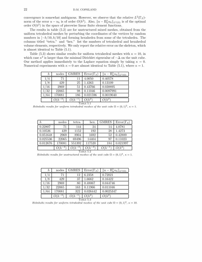
22 D.M. COPELAND

convergence is somewhat ambiguous. However, we observe that the relative L2(ΓS)-norm of the error u − uh is of order O(h2). Also, ‖u− Π1

huh‖L2(Ω) is of the optimalorder O(h2) in the space of piecewise linear finite element functions.

The results in table (5.2) are for unstructured mixed meshes, obtained from theuniform tetrahedral meshes by perturbing the coordinates of the vertices by randomnumbers in [−h/10, h/10] and forming hexahedra from some of the tetrahedra. Thecolumns titled “tetra.” and “hex.” list the numbers of tetrahedral and hexahedralvolume elements, respectively. We only report the relative error on the skeleton, whichis almost identical to Table (5.1).

Table (5.3) shows similar results for uniform tetrahedral meshes with κ = 10, inwhich case κ2 is larger than the minimal Dirichlet eigenvalue of −∆ on the unit cube.Our method applies immediately to the Laplace equation simply by taking κ = 0.Numerical experiments with κ = 0 are almost identical to Table (5.1), where κ = 1.

h nodes GMRES Error(ΓS) ‖u− Π1huh‖L2(Ω)

1/4 71 11 4.0050 0.405781/8 429 25 1.4263 0.13109

1/16 2969 51 0.43766 0.0388951/32 22065 98 0.11046 0.00979911/64 170081 186 0.021596 0.0019040

O(h−3) O(h−1) O(h2) O(h2)Table 5.1

Helmholtz results for uniform tetrahedral meshes of the unit cube Ω = (0, 1)3, κ = 1.

h nodes tetra. hex. GMRES Error(ΓS)

0.22807 71 144 24 14 4.07810.10526 429 1152 192 28 1.42730.051648 2969 8904 1692 52 0.428890.025536 22065 69496 14404 97 0.110230.012676 170081 551392 117520 184 0.021997

O(h−3) O(h−3) O(h−3) O(h−1) O(h2)Table 5.2

Helmholtz results for unstructured meshes of the unit cube Ω = (0, 1)3, κ = 1.

h nodes GMRES Error(ΓS) ‖u− Π1huh‖L2(Ω)

1/4 71 12 6.2358 0.720211/8 429 37 1.6662 0.16422

1/16 2969 80 0.48067 0.0447461/32 22065 163 0.11966 0.0110461/64 170081 322 0.026442 0.0025347

O(h−3) O(h−1) O(h2) O(h2)Table 5.3

Helmholtz results for uniform tetrahedral meshes of the unit cube Ω = (0, 1)3, κ = 10.

BOUNDARY-ELEMENT-BASED FINITE ELEMENT METHODS 23

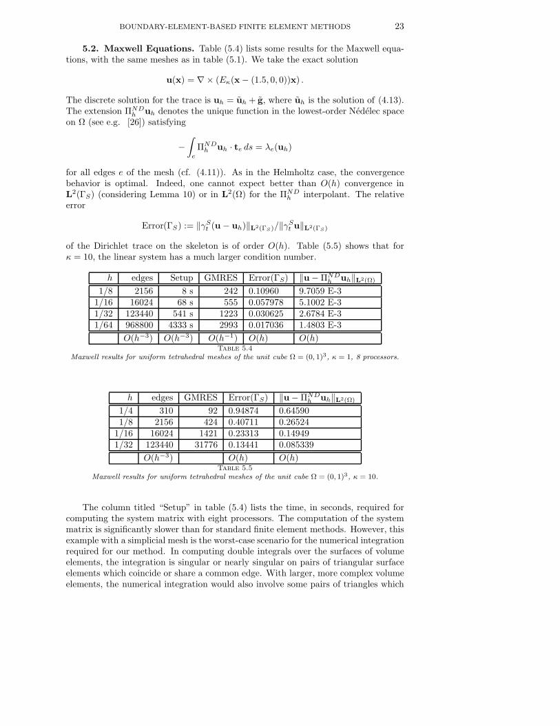
5.2. Maxwell Equations. Table (5.4) lists some results for the Maxwell equa-tions, with the same meshes as in table (5.1). We take the exact solution

u(x) = ∇× (Eκ(x − (1.5, 0, 0))x) .

The discrete solution for the trace is uh = uh + g, where uh is the solution of (4.13).The extension ΠND

h uh denotes the unique function in the lowest-order Nedelec spaceon Ω (see e.g. [26]) satisfying

−

∫

e

ΠNDh uh · te ds = λe(uh)

for all edges e of the mesh (cf. (4.11)). As in the Helmholtz case, the convergencebehavior is optimal. Indeed, one cannot expect better than O(h) convergence inL2(ΓS) (considering Lemma 10) or in L2(Ω) for the ΠND

h interpolant. The relativeerror

Error(ΓS) := ‖γSt (u − uh)‖L2(ΓS)/‖γ

St u‖L2(ΓS)

of the Dirichlet trace on the skeleton is of order O(h). Table (5.5) shows that forκ = 10, the linear system has a much larger condition number.

h edges Setup GMRES Error(ΓS) ‖u− ΠNDh uh‖L2(Ω)

1/8 2156 8 s 242 0.10960 9.7059 E-31/16 16024 68 s 555 0.057978 5.1002 E-31/32 123440 541 s 1223 0.030625 2.6784 E-31/64 968800 4333 s 2993 0.017036 1.4803 E-3

O(h−3) O(h−3) O(h−1) O(h) O(h)Table 5.4

Maxwell results for uniform tetrahedral meshes of the unit cube Ω = (0, 1)3, κ = 1, 8 processors.

h edges GMRES Error(ΓS) ‖u− ΠNDh uh‖L2(Ω)

1/4 310 92 0.94874 0.645901/8 2156 424 0.40711 0.26524

1/16 16024 1421 0.23313 0.149491/32 123440 31776 0.13441 0.085339

O(h−3) O(h) O(h)Table 5.5

Maxwell results for uniform tetrahedral meshes of the unit cube Ω = (0, 1)3, κ = 10.

The column titled “Setup” in table (5.4) lists the time, in seconds, required forcomputing the system matrix with eight processors. The computation of the systemmatrix is significantly slower than for standard finite element methods. However, thisexample with a simplicial mesh is the worst-case scenario for the numerical integrationrequired for our method. In computing double integrals over the surfaces of volumeelements, the integration is singular or nearly singular on pairs of triangular surfaceelements which coincide or share a common edge. With larger, more complex volumeelements, the numerical integration would also involve some pairs of triangles which

24 D.M. COPELAND

are sufficiently far apart to allow for much faster, lower-order quadrature rules. Thusany comparison of setup times would be strongly biased in favor of standard finiteelement methods.

Although the methods of this paper can theoretically be applied with piecewiseconstant κ, we do not report numerical experiments for such cases, since an exactsolution is unknown. Experiments with varying κ could only show a growth in theiteration numbers, as a preconditioner has not yet been proposed.

A very important consideration for numerical performance, out of the scope ofthis paper, is the optimal choice of the element size. In the context of boundary-element-based finite element methods, elements and subdomains are theoretically in-terchangeable, so elements may be of any size as long as they resolve jumps in thewavenumber. Increasing the element size would decrease the size of the mesh skeletonand therefore the number of unknowns in the discrete system. Also, the numericalintegration would involve fewer singular integrals, reducing much of the computa-tional bottleneck. The negative computational effects of increasing the element sizeare that the dense local matrices become larger and the matrix inversion involvedin their computation becomes more expensive. At some point, special boundary ele-ment techniques to obtain data-sparse matrices would become necessary. However, itseems plausible that the numerical performance could be improved by balancing thereduction in the system size with the cost of larger element matrices.

6. Conclusions and Outlook. We have introduced new finite element meth-ods which can be applied to general polyhedral meshes, with piecewise constant co-efficients. The error behavior has been shown theoretically to be quasi-optimal forthe pure domain decomposition case with subdomains of fixed size. Although wedid not perform numerical experiments demonstrating the theoretical convergencerates, we have confirmed that the L2(Ω) convergence rates for both the Helmholtzand Maxwell methods are of the same order as for standard finite element methods onsimple meshes. Thus the methods have good convergence rates and are more generallyapplicable than conventional methods.

It is evident from the previous section that this work is only the beginning, asseveral critical computational issues need to be addressed. To obtain better accuracy,techniques should be developed to utilize the representation formulas to computean approximate solution in Ω. Perhaps more important in practice is the need fora preconditioner that is robust with respect to the size of the wavenumber and itsjumps. Also, it would be interesting to investigate the advantages in performancethat might be attained by taking larger elements.

7. Acknowledgements. The author gratefully acknowledges Prof. U. Langerand D. Pusch for many productive discussions which motivated this paper. Manythanks are also due to G. Of and M. Windisch for their assistance with a boundaryelement code. This work was supported by the Austrian Science Fund (FWF), projectP19255-N18.

REFERENCES

[1] R.A. Adams, Sobolev spaces, Academic Press [A subsidiary of Harcourt Brace Jovanovich,Publishers], New York-London, 1975. Pure and Applied Mathematics, Vol. 65.

[2] M. Bebendorf, Approximation of boundary element matrices, Numer. Math., 86 (2000),pp. 565–589.

BOUNDARY-ELEMENT-BASED FINITE ELEMENT METHODS 25

[3] F. Brezzi, K. Lipnikov, and M. Shashkov, Convergence of the mimetic finite difference

method for diffusion problems on polyhedral meshes, SIAM J. Numer. Anal., 43 (2005),pp. 1872–1896 (electronic).

[4] A. Buffa and S. H. Christiansen, The electric field integral equation on Lipschitz screens:

definitions and numerical approximation, Numer. Math., 94 (2003), pp. 229–267.[5] A. Buffa and P. Ciarlet, Jr., On traces for functional spaces related to Maxwell’s equations.

I. An integration by parts formula in Lipschitz polyhedra, Math. Methods Appl. Sci., 24(2001), pp. 9–30.

[6] , On traces for functional spaces related to Maxwell’s equations. II. Hodge decompositions

on the boundary of Lipschitz polyhedra and applications, Math. Methods Appl. Sci., 24(2001), pp. 31–48.

[7] A. Buffa, M. Costabel, and C. Schwab, Boundary element methods for Maxwell’s equations

on non-smooth domains, Numer. Math., 92 (2002), pp. 679–710.[8] A. Buffa, M. Costabel, and D. Sheen, On traces for H(curl,Ω) in Lipschitz domains, J.

Math. Anal. Appl., 276 (2002), pp. 845–867.[9] A. Buffa and R. Hiptmair, Galerkin boundary element methods for electromagnetic scatter-

ing, in Topics in computational wave propagation, vol. 31 of Lect. Notes Comput. Sci.Eng., Springer, Berlin, 2003, pp. 83–124.

[10] , A coercive combined field integral equation for electromagnetic scattering, SIAM J.Numer. Anal., 42 (2004), pp. 621–640 (electronic).

[11] , Regularized combined field integral equations, Numer. Math., 100 (2005), pp. 1–19.[12] A. Buffa, R. Hiptmair, T. von Petersdorff, and C. Schwab, Boundary element meth-

ods for Maxwell transmission problems in Lipschitz domains, Numer. Math., 95 (2003),pp. 459–485.

[13] M. Costabel, Boundary integral operators on Lipschitz domains: elementary results, SIAMJ. Math. Anal., 19 (1988), pp. 613–626.

[14] V. Dolean, H. Fol, S. Lanteri, and R. Perrussel, Solution of the time-harmonic Maxwell

equations using discontinuous Galerkin methods, J. Comput. Appl. Math. (to appear),(2007).

[15] S. Erichsen and S.A. Sauter, Efficient automatic quadrature in 3-d Galerkin BEM, Comput.Methods Appl. Mech. Engrg., 157 (1998), pp. 215–224. Seventh Conference on NumericalMethods and Computational Mechanics in Science and Engineering (NMCM 96) (Miskolc).

[16] W. Hackbusch, A sparse matrix arithmetic based on H-matrices. I. Introduction to H-

matrices, Computing, 62 (1999), pp. 89–108.[17] R. Hiptmair, Coupling of finite elements and boundary elements in electromagnetic scattering,

SIAM J. Numer. Anal., 41 (2003), pp. 919–944 (electronic).[18] R. Hiptmair and P. Meury, Stabilized FEM-BEM coupling for Helmholtz transmission prob-

lems, SIAM J. Numer. Anal., 44 (2006), pp. 2107–2130 (electronic).[19] P. Houston, I. Perugia, A. Schneebeli, and D. Schotzau, Interior penalty method for the

indefinite time-harmonic Maxwell equations, Numer. Math., 100 (2005), pp. 485–518.[20] , Mixed discontinuous Galerkin approximation of the Maxwell operator: the indefinite

case, M2AN Math. Model. Numer. Anal., 39 (2005), pp. 727–753.[21] G. C. Hsiao, O. Steinbach, and W. L. Wendland, Domain decomposition methods via

boundary integral equations, J. Comput. Appl. Math., 125 (2000), pp. 521–537. Numericalanalysis 2000, Vol. VI, Ordinary differential equations and integral equations.

[22] J.M. Hyman and M. Shashkov, Mimetic discretizations for Maxwell’s equations, J. Comput.Phys., 151 (1999), pp. 881–909.

[23] Y. Kuznetsov, K. Lipnikov, and M. Shashkov, The mimetic finite difference method on

polygonal meshes for diffusion-type problems, Comput. Geosci., 8 (2004), pp. 301–324(2005).

[24] K. Lipnikov, M. Shashkov, and D. Svyatskiy, The mimetic finite difference discretization

of diffusion problem on unstructured polyhedral meshes, J. Comput. Phys., 211 (2006),pp. 473–491.

[25] W. McLean, Strongly elliptic systems and boundary integral equations, Cambridge UniversityPress, Cambridge, 2000.

[26] P. Monk, Finite element methods for Maxwell’s equations, Numerical Mathematics and Sci-entific Computation, Oxford University Press, New York, 2003.

[27] O. Steinbach, Numerical approximation methods for elliptic boundary value problems,Springer, New York, 2008. Finite and boundary elements, Translated from the 2003 Ger-man original.