A

IPhiofltit©

K

1

biih[r

f

0

Available online at www.sciencedirect.com

Mathematics and Computers in Simulation 87 (2013) 19–29

Original article

Bootstrap tests for fractional integration and cointegration:A comparison study

G.C. Franco a,∗, V.A. Reisen b, F.A. Alves a

a Departamento de Estatistica, UFMG, Av. Antônio Carlos, 6627, Belo Horizonte 31270-901, Brazilb Departamento de Estatistica, PPGEA, UFES, Av. Fernando Ferrari, s/n – Vitória 29065-900, Brazil

Received 20 December 2011; received in revised form 14 September 2012; accepted 16 November 2012Available online 9 February 2013

bstract

There are few methods in the literature to test for integration and cointegration in the traditional framework, i.e. using the(0)–I(1) paradigm. In the first case, the most known are the Dickey–Fuller (DF), the Augmented Dickey–Fuller (ADF) and thehillips–Perron (PP) tests, while in the latter case, the Engle and Granger (EG) and Johansen procedures are broadly used. Butow well do these methods perform when the underlying process presents the long-memory characteristic? The bootstrap techniques used here to approximate the distribution of integration and cointegration test statistics based on a semiparametric estimatorf the fractional parameter of ARFIMA(p,d,q) models. The proposed bootstrap tests, along with the asymptotic test based on theractional semiparametric estimator, are empirically compared to the standard tests, for testing integration and cointegration in theong-memory context. Monte Carlo simulations are performed to evaluate the size and power of the tests. The results show thathe conventional tests, except for the procedures based on the DF approach, loose power when compared to fractional tests. As anllustration, the tests were applied to the series of Ibovespa (Brazil) and Dow Jones (USA) indexes and led to the conclusion thathese series do not share a long-run relationship.

2013 IMACS. Published by Elsevier B.V. All rights reserved.

eywords: ARFIMA model; Semiparametric estimator; Classical unit root tests; EG and Johansen tests; Bootstrap

. Introduction

To study the relationship among economic variables, the concept of cointegration, introduced by Granger [12], haseen widely employed, mainly because of the spurious regression problem. The basic idea of cointegration consistsn the fact that if each series forming a vector {Xt}t=1,2,... is nonstationary, but some linear combination of the seriess stationary, the series are said to be cointegrated. Since the pioneer work of [12], several studies about this topic

ave been developed. In the classic context, the most used tests for cointegration are the Engle–Granger (EG) test8], the Phillips–Ouliaris test [27] and the Johansen procedure [19]. Besides, tests to verify the presence of a unitoot are necessary to use appropriate procedures for modeling the data. Among the most used unit root tests are the

∗ Corresponding author at: Av. Antônio Carlos, 6627, Pampulha, Belo Horizonte 31270-901, MG, Brazil. Tel.: +55 31 34095949;ax: +55 31 34095924.

E-mail address: glauraf@ufmg.br (G.C. Franco).

378-4754/$36.00 © 2013 IMACS. Published by Elsevier B.V. All rights reserved.http://dx.doi.org/10.1016/j.matcom.2012.11.011

20 G.C. Franco et al. / Mathematics and Computers in Simulation 87 (2013) 19–29

Dickey–Fuller (DF) test [4], the Augmented Dickey–Fuller (ADF) test [31] and the nonparametric test of Phillips andPerron (PP) [28], which test the null hypothesis of nonstationarity. By the other hand, there are tests that verify thestationarity of the series, such as the Kwiatkowski–Phillips–Schmidt–Shin (KPSS) test [22].

However, do the classical procedures work well if the data under study are generated by a long-memory process?Many authors have studied the power of classical unit root tests against fractional alternatives (see [6,20]). Hassler andWolters [14] present an extensive empirical study on the power of the most known classical unit root tests and haveconcluded that the ADF test performs poorly when applied to fractionally integrated time series, while the DF and PPtests present very satisfactory results, with the DF being slightly superior to the PP test.

Recently, several approaches appeared in researches related to the fractional cointegration topic. Different method-ologies are being implemented in the estimation and construction of hypothesis tests concerning fractional processes.Ref. [21] tests the hypothesis of no cointegration when residuals are fractionally cointegrated and the cointegrationrelation has to be estimated. The fractional autoregressive moving average, ARFIMA(p,d,q), model (see [15]) has beenwidely used to this purpose, due to the fact that the fractional parameter d can capture the memory of a series, and itsvarious estimators can be used in hypothesis tests for fractionally cointegrated processes (see, for example [7,32]). Thesemiparametric estimator proposed by [11], called here GPH, is one of the most used methods to estimate the memoryparameter, d. Recent developments in the estimation of ARFIMA models can be found in [30].

The problems stated above can be still worse if the size of the series is small, as in this case asymptotic tests maybe compromised. Thus, in this work bootstrap tests under the fractional approach are proposed in the unit root andcointegration contexts, with the resampling performed in the residuals of the fitted model [9]. Asymptotic propertiesof bootstrap methods for long-memory processes can be found in very few works, as the results of [1] and [29].Nevertheless, the bootstrap is used to construct empirical hypothesis tests in this framework (see [2,10]).

Thus the main objective of this work is to compare the power of the bootstrap tests proposed here with classicaland fractional unit root and cointegration tests, when the underlying generating process presents the long-memorycharacteristic. To attain the above purpose, a broad Monte Carlo study is performed to compare, empirically, thesize and power of some fractional tests with the classical ones, obtained using the main methodologies existent inthe literature. In the classical approach the tests to be compared are the DF, ADF and PP, for unit root, and EG andJohansen, for cointegration, while in the fractional approach the tests used, both in the unit root and cointegrationcontexts, are the asymptotic and the proposed bootstrap tests based on the GPH estimator.

The paper is structured as follows. In Section 2 the ARFIMA model and the tests for unit roots are presented. Thecointegration topic is treated in Section 3, as well as the tests employed in this work to check for cointegration amongtwo or more time series. A Monte Carlo study comparing the size and power of the tests is presented in Section 4.Section 5 shows an application to a real time series and Section 6 concludes the work.

2. Fractional integration

A time series {Xt}t=1,2,... possesses the long-memory characteristic if its spectral density, f(ω), is approximatelywritten by

f (ω)∼C|ω|−d, when ω → 0, (2.1)

where C is a non zero constant, ω ∈ (−π,π) and d ∈ �.A class of models that has a spectral representation with the property given in (2.1) is called fractionally integrated

autoregressive moving average (ARFIMA) process (see [15]) and can be written as

xt = (1 − B)−dUt, (2.2)

−1 2

where Ut = θq(B)φp (B)εt , {εt}t=1,2,... is a white noise process with zero mean and constant variance σε , φp (B) and

θp (B) are polynomials in B with all roots outside the unit circle and B is the backshift operator of the form Bkxt = xt−k.For positive d the process is said to have long memory and, when d = 0 or d < 0, xt is said to be short or intermediatememory (anti-persistent), respectively (see, for example [16]).

w

pCw

2

2

It

wD

tt

v

2

c

w

tit

2

2

opnUa

G.C. Franco et al. / Mathematics and Computers in Simulation 87 (2013) 19–29 21

The term (1 − B)d in expression (2.2) can be obtained by

(1 − B)d =∞∑

j=1

�(j − d)

�(−d)�(j + 1)Bj

here �(a) = ∫ ∞0 xa−1e−xdx is the Digamma function.

The main features of the ARFIMA model can be established based on the value of the fractional parameter d. Arocess is said to be integrated of order d, or I(d), if it needs to be differentiated d times to become stationary [8].onventional tests to check for the order of integration in a time series, also known as unit root tests, encompass aide variety of tests. In this section, a brief description of the unit root tests used in this study is presented.

.1. Classical tests for unit root

.1.1. Dickey–Fuller (DF) and Augmented Dickey–Fuller (ADF) testsThe DF and ADF tests, proposed by [4] and [31], respectively, test the null hypothesis that a time series {yt}t=1,2,... is

(1) against the alternative that it is I(0). Assuming that the dynamics of a sample y1, y2,. . .,yn have an AR(p) structure,he ADF test is based on estimating the regression

yt = (ρ − 1)yt−1 +p∑

i=1

θiyt−i + et, t = 1, . . . , n, (2.3)

here yt = yt − yt−1 and et is a white noise process with zero mean, constant variance σ2e , and finite fourth moment. The

F test is based on the same regression (2.3), but only with the AR(1) component, i.e. without the term∑p

i=1θiyt−i.The ADF test requires the order p to be considered in the regression Eq. (2.3). There are many works in the literature

hat report studies related to this. As an example, the paper of [5] sets the number of lags equal to n0.25. In this work,he order p is calculated using the Akaike Information Criteria (AIC).

Under the null hypothesis, ρ = 1, and some model conditions, the usual t-statistic can be employed, with criticalalues calculated empirically by [4] for the DF and [31] for the ADF statistic, using results from the Brownian motion.

.1.2. Phillips–Perron unit root tests (PP)The PP test, proposed by [28], also tests the null hypothesis that a time series is I(1) against the alternative I(0). It

onsists on fitting the following regression,

yt = (ρ − 1)yt−1 + ut, t = 1, . . . , n, (2.4)

here ut is I(0) and may be heteroscedastic.The main characteristic of the PP test is to correct for any serial correlation and heteroscedasticity in the errors of

he test regression by directly modifying the test statistic. Thus, this test is robust to general forms of heteroscedasticityn the error term ut in Eq. (2.4). Another advantage of the PP test is that it is not necessary to specify a lag length forhe test regression.

.2. Fractional tests for unit root

.2.1. Asymptotic test based on the GPH estimatorThe procedure introduced by Geweke and Porter-Hudak [11], denoted here GPH, can be used as a simple way

f testing the presence of a unit root in the long-memory context. This method employs the ordinary least square

rocedure on the spectral function of the ARFIMA model given in (2.2) to estimate parameter d. For a sample of size

of process (2.2), the number of observations in the regression equation (the bandwidth) is a function of n, say g(n).nder some conditions, Ref. [16] proved that the GPH method is a consistent estimator of the memory parameter and

symptotically normal for Gaussian time series processes.

22 G.C. Franco et al. / Mathematics and Computers in Simulation 87 (2013) 19–29

The consistency of the GPH estimator, when d = 1, is proved by [26]. The author shows that, under some conditions,this estimator has, asymptotically, the following mixed normal limit distribution

√g(n)(dGPH − d)

D−→MN

(0,

σ2(W)

4

),

where W is χ21, σ2(w) = Var[log χ2

2(2w)], with χ22(γ) denoting a χ2

2 distribution with noncentrality parameter γ andthe optimal g(n) is of order o (n4/5) (see [28]).

As it has often been reported in the long-memory literature, the short-memory component causes significant bias inthe estimator of the long-memory parameter, especially if the bandwidth is not properly set (see, for example [17,30]among others). When there is no short memory component in the ARFIMA model, the plot of the log periodogramversus log(2 sin ωj/2), ωj = (2πj)/n and j = 1, ..., g(n), is essentially a straight line for all frequencies. In thissituation, increasing the bandwidth to g(n) = n/2 − 1 gives more precise estimates, that is, the variance is reduced.

Based on the above arguments, the GPH estimator can be used for testing unit roots. Thus, to test the null hypothesisH0: d = 1 against H1: d < 1, based on the asymptotic distribution of the GPH estimator, the test statistic is given by

t = dGPH − 1

σdGPH

, (2.5)

where σdGPHis the standard error of the GPH estimator (see [11]). Critical values for the test statistic (2.5), for different

sample sizes, can be found in [32].

2.2.2. Bootstrap test based on the GPH estimatorTests based on the asymptotic properties of a test statistic can loose power when applied to a real data set. An

alternative to this is to use bootstrap tests, which possess size-distortion of order n−1/2 for iid processes, smaller thanthat of the corresponding asymptotic test (see [3]). Therefore, the bootstrap can be used to estimate the small-sampledistribution of the test statistic, leading to more reliable inference in finite samples.

In this work the bootstrap in the residuals of the fitted ARFIMA model is employed (see [9] for more details).Nevertheless, the findings of the bootstrap methods discussed here are only empirical, that is, the paper does not havethe aim to give a theoretical justification of these methods.

Consider the ARFIMA(p,d,q) process given in (2.2). For a series of size n, parameters φp, θq and d can be estimatedto calculate the sample residuals. The bootstrap residuals, ε∗

t , are thus obtained after centering and resampling, withreplacement, the sample residuals. Therefore, it is possible to build recursively the bootstrap series x∗

t from ε∗t in the

following way

x∗t = θq(B)φ−1

p (B)(1 − B)−d ε∗t , t = 1, . . . , n. (2.6)

To test the hypothesis H0: d = 1 against H1: d < 1, two different bootstrap tests will be used. The first one, denotedhere Bd, employs, as the test statistic, the estimate of d obtained by the GPH procedure. The second test, called BReg,uses the GPH estimate of d divided by its ordinary least square (OLS) standard error. The finite-sample data generatingprocess (DGP) under the null hypothesis can be estimated using the bootstrap.

The steps to calculate the bootstrap tests are the following:

1) Calculate the test statistic, τn, for the original sample.2) Generate B bootstrap series X∗

1, X∗2, ..., X∗

B, where X∗i = (x∗

1, ..., x∗n), i = 1,. . .,B, under the null hypothesis, H0:

d = 1.3) For each bootstrap sample, calculate the value of the test statistic, τ∗

n .4) Approximate the empirical distribution of the test statistic, Fτn (a), by the bootstrap distribution function,

Fτ∗n(a) = B−1

B∑b=1

1{τ∗n ≤ a} (2.7)

56

Di

t

3

f

Dc0

{b

to

ei

w

it

p

3

3

oae

pttE

G.C. Franco et al. / Mathematics and Computers in Simulation 87 (2013) 19–29 23

) Calculate critical values for the bootstrap test from (2.7), for an α level.) If the value of the test statistic for the original sample is smaller than the critical value obtained in Step (5), reject

the null hypothesis (the series do not present a unit root).

Remark. For iid and weak dependent cases, the distribution of τ∗n , under the probability law induced by the bootstrap

GP, approximates the distribution of τn in the original DGP. Thus, Fτ∗n(a) can be a good approximation to Fτn (·) if B

s sufficiently large [29].The above remark is a general result which states that, under some conditions, the distribution of bootstrap unit root

ests converges to the same limit distribution as the standard test statistics (see [24]).

. Fractional cointegration

The classical Engle and Granger [8] definition for cointegration can be extended for the fractional cointegrationramework in the following way (see [7]).

efinition 3.1. Let {Xt}t=1,2,.. be a vector of k series xit, such that xit ∼ I(di), di > 0, i = 1,. . .,k. {Xt} is called fractionallyointegrated, denoted by Xt∼FCI(d1, ..., dk; du), if there exists a k × 1 vector δ /= 0 such that ut = δ′Xt∼I(du), where

< du < min1≤i≤kdi.

This definition is valid if, and only if, di = dj for any δ /= j, that is, cointegration requires at least two elements ofXt} to share the same long-memory parameter. If d1 = d2 = ... = dk = d, it is usual to write Xt∼CI(d, b), where

= d − du measures the strength of the cointegration relation.Classical cointegration is a particular case of Definition 3.1, where d = b = 1. The relevant case in this study is when

he components of vector {Xt}t=1,2,...,n are I(1), but the cointegration error is I(1 − b), with b > 0, that is, the integrationrder can assume a noninteger value.

In what follows, x1t is assumed to be the scalar response variable and zt = (x2t , ..., xkt) the vector of (k − 1)xplanatory variables, thus {Xt}t=1,2,...,n can be partitioned as Xt = (x1t , z′

t)′. If vector {Xt}t=1,2,...,n is cointegrated,

t is possible to fit a regression of the type

x1t = β′zt + ut, t = 1, ..., n (3.1)

here ut is I(du), with du < di, i = 1,. . .,k.Assuming, for simplicity, that d1 = d2 = ... = dk = d, the null hypothesis of noncointegration under test is H0:b = 0,

mplying that ut ∼ I(d) for any choice of vector β. Under the alternative hypothesis, b > 0, there exists a vector β suchhat ut ∼ I(d − b).

This section describes the cointegration tests compared in this study, that is, the Engle–Granger test [8], the Johansenrocedure [19], the test based on the asymptotic distribution of the GPH estimator and the bootstrap tests.

.1. Classical tests for cointegration (or noncointegration)

.1.1. Engle and Granger methodAssume that {Yt} = {y1t , ..., ykt}, t = 1,. . .,n, can be represented as a k-dimensional autoregressive vector (VAR) of

rder p. The Engle and Granger test [8], also known as EG test, consists in running the static regression given in (3.1),fter having verified that {yit}i=1,...,n, i = 1, ..., k are each of them I(1) variables. The next step in the EG test is tostimate the k × 1 vector β by OLS and then to perform a unit root test in

ut = y1t − β′zt, t = 1, . . . , n (3.2)

The distribution of the test statistic under the null is affected by the number of regressors included in (3.2), the

resence of trend in the series and the estimation of vector β. Therefore, different critical values are necessary whenhe number of regressors changes or in the presence of trends. Mackinnon [23] built critical values for particular tests,aking into consideration the number of regressors and the presence or absence of constant and trend components. TheG test can be found in many textbooks, such as [13] and [25].

24 G.C. Franco et al. / Mathematics and Computers in Simulation 87 (2013) 19–29

3.1.2. Johansen procedureFor a cointegrated VAR model, {Yt} = {y1t , ..., ykt}, t = 1,. . .,n, with r cointegrating factors (r < k), the error-correction

model (ECM) can be written as:

Yt = �Yt−k +k−1∑i=1

�iYt−i + ΦDt + μ + εt,

where �i = −∑pj=i+1φj is the matrix of short run coefficients and � = ∑p

i=1φi − In = −φ(1) is the matrix of longrun coefficients. Dt are seasonal dummies orthogonal to the constant term, μ. Additionally, εt, t = 1, ..., n, areindependent k-dimensional Gaussian variables with zero mean and constant variance. For more details, see [18].

Johansen and Juselius [19] have proposed a procedure using the maximum likelihood method based on the multivari-ate normal assumption. This method consists in testing if the coefficients of matrix � contain the long run informationabout the variables under study.

The hypotheses of the tests are H0: Rank(�) = r versus H1: Rank(�) > r. The tests are based on the eigenvaluesassociated to matrix � and can be performed using two likelihood tests: trace and maximum value. Critical values forboth tests must be calculated through simulation and can be found in [13].

3.2. Fractional tests for cointegration (or non cointegration)

3.2.1. Asymptotic test based on the GPH estimatorTo perform the GPH cointegration test, it is necessary to check if at least two series in vector {Xt}t=1,2,...,n present

the same order of integration, d. Next, a regression model is fitted to the series and the OLS residuals, given in Eq.(3.1), are calculated.

To test the null hypothesis of noncointegration, H0: ut ∼ I(1) against H1: ut ∼ I(d − b), b > 0, based on the asymptoticdistribution of the GPH estimator [11], the test statistic is given by,

t = dGPH − 1

σdGPH

(3.3)

where dGPH is the GPH estimate of d − b applied to the OLS residuals and σdGPHis its asymptotic standard deviation.

Critical values for the test statistic (3.3) can be found in [32].

3.2.2. Bootstrap test based on the GPH estimatorThe logic behind bootstrap tests is the same as the asymptotic test for cointegration. Thus, to perform bootstrap tests

it is also necessary to check if at least two series in vector {Xt}t=1,2,...,n, defined in (3.1), present the same order. If thisis true, the residuals of the regression model fitted to the series are calculated as in (3.2) to test the null hypothesis ofnoncointegration, H0: ut ∼ I(1) against H1: ut ∼ I(d − b), b > 0.

The bootstrap tests are built in the same way described for unit root tests. The two bootstrap tests, Bd and BReg,are also calculated here, but this time based on the GPH estimator of d − b, applied to the OLS residuals. The steps areas follows:

1) Calculate the test statistic, τn, for the residual series.2) Generate B bootstrap residual series under the null hypothesis, H0: d = 1.3) For each bootstrap sample, calculate the value of the test statistic, τ∗

n .4) Approximated Fτn (a) by the bootstrap distribution function, Fτ∗

n(a).

5) Calculate the critical values for the bootstrap test, at the α level.6) If the value of the test statistic for the original sample is smaller than the critical value obtained in Step (5) the null

hypothesis is rejected (the series do not present a unit root).

4. Simulation results

To compare the performance of the unit root and cointegration tests described in the previous sections, 1000 seriesxi,t, i = 1,2, t = 1,. . .,n, of sizes n = 100 and 500 were generated from the ARFIMA(0,d,0) model, d ∈ [0.1,1.0], with {εt}

G.C. Franco et al. / Mathematics and Computers in Simulation 87 (2013) 19–29 25

Table 1Power function for the unit root tests (n = 100).

d ADF DF PP GPHn/2 BRegn/2 Bdn/2 GPH0.7 BReg0.7 Bd0.7

0.1 97.8 100 100 100 100 100 100 100 1000.2 96.4 100 100 100 100 100 100 100 1000.3 86.0 100 100 100 100 100 100 99.8 99.70.4 73.8 100 100 100 100 100 98.8 97.2 98.40.5 54.8 99.6 99.3 99.8 99.7 99.6 91.3 85.6 92.50.6 36.4 93.4 89.3 95.5 95.4 93.1 76.2 67.3 76.30.7 22.4 71.7 61.6 73.6 73.2 67.5 50.0 41.2 52.90.8 11.4 37.5 32.1 40.6 41.5 35.7 24.9 17.7 30.00.9 8.2 15.1 14.2 15.8 16.4 12.4 11.5 8.4 11.61

boswewrg

4

p(B

S

GB

foiti

psa

4

b(e

5.5 4.8 5.9 4.8 3.4 7.0 4.9 3.2 5.1

eing a Gaussian white noise process with zero-mean and unit variance. Two bandwidths were used in the calculationf the GPH estimator. The first one utilizes g(n) = n/2−1 observations available in the periodogram function, while theecond one uses only part of the information, and is given by g(n) = n0.7. These bandwidth choices were here consideredith the aim to check the finite property of the bandwidth on the estimates and on the convergence of the standardized

stimator to the normal distribution, according to the discussion pointed out in Section 2.2. Nominal sizes for the testsere fixed at α = 5% and a size correction was performed for all tests that presented size too small or too large with

espect to the 5% level. The bootstrap replications were fixed at 1000. The samples were simulated using the dataeneration method given in [15] through the IMSLFORTRAN subroutines.

.1. Size and power of unit root tests

The objective of this section is to compare the performance of the unit root tests presented in Section 2, through theower and size of the test statistics considered. The tests are the Dickey–Fuller (DF), the Augmented Dickey–FullerADF), the Phillips–Perron (PP) and the asymptotic (GPH) and bootstrap tests (BReg and Bd). In the tables, GPHn/2,Regn/2, Bdn/2 and GPH0.7, BReg0.7, Bd0.7 are the estimates for g(n) = n/2−1 and g(n) = n0.7, respectively.

The null hypothesis to be considered is H0 : x1t∼I(1), that is, the series presents a unit root. As already cited inection 2.1, the AIC criterion was used in the ADF test to choose the order p in the autoregression.

Table 1 shows the size and power of the tests, for n = 100, considering a nominal level of 5%. The DF, GPHn/2,PH0.7 and Bd0.7 are the tests that present empirical sizes closer to the 5% fixed level, followed by the ADF. TheRegn/2 and BReg0.7 are the most conservative tests, while the Bdn/2 and PP are less conservative.

With respect to the power, it can be seen that the test with the worst performance is the ADF test, followed by theractional tests with bandwidth g(n) = n0.7. The DF and the fractional tests with bandwidth g(n) = n/2−1 are the bestnes and present a similar behavior, while the PP test shows power slightly smaller than this last group. The differencen power found for the fractional tests was expected in this case, since there are many results in the literature showinghat the maximum bandwidth produces estimates which are more accurate for ARFIMA(0,d,0) processes, as discussedn Section 2.2.

For series of size n = 500 (Table 2), the behavior of the tests is very similar to the case n = 100. As expected, theower of the tests increases, being very close to 100% for values of d up to 0.6, except for the ADF test. The PP testhows power slightly inferior to the fractional tests with bandwidth g(n) = n0.7. The tests with larger power functionre the fractional ones with bandwidth g(n) = n/2−1.

.2. Size and power for the noncointegration tests

In this section, the cointegration tests described in Section 3 are compared building a noncointegration relation

etween two series, x1t and x2t. The procedures are the Engle–Granger test based on AR(1) and AR(p) representationsEG1 and EGp, respectively), the Johansen test (Johan), the test based on the asymptotic distribution of the GPHstimator (GPHn/2 and GPH0.7) and the bootstrap tests (BRegn/2, Bdn/2, BReg0.7 and Bd0.7).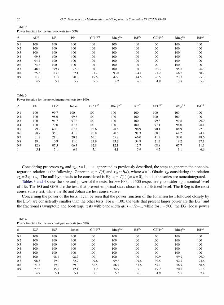

26 G.C. Franco et al. / Mathematics and Computers in Simulation 87 (2013) 19–29

Table 2Power function for the unit root tests (n = 500).

d ADF DF PP GPHn/2 BRegn/2 Bdn/2 GPH0.7 BReg0.7 Bd0.7

0.1 100 100 100 100 100 100 100 100 1000.2 100 100 100 100 100 100 100 100 1000.3 100 100 100 100 100 100 100 100 1000.4 99.8 100 100 100 100 100 100 100 1000.5 94.2 100 100 100 100 100 100 100 1000.6 74.6 100 100 100 100 100 100 100 1000.7 48.2 99.7 97.0 100 100 100 96.3 95.8 96.30.8 25.3 83.8 62.1 93.2 93.8 94.1 71.2 66.2 68.70.9 11.0 31.2 20.8 45.6 42.6 44.6 26.5 23.3 25.31 4.7 5.2 5.7 5.0 4.2 6.2 4.9 3.8 5.2

Table 3Power function for the noncointegration tests (n = 100).

d EG1 EGp Johan GPHn/2 BRegn/2 Bdn/2 GPH0.7 BReg0.7 Bd0.7

0.1 100 99.7 100 100 100 100 100 100 1000.2 100 98.6 99.8 100 100 100 100 100 1000.3 100 94.7 97.6 100 100 100 99.8 99.8 99.90.4 100 79.0 87.3 100 100 100 97.1 96.0 98.10.5 99.2 60.1 67.3 98.6 98.6 98.9 90.1 86.9 92.30.6 88.7 35.1 41.5 90.8 90.5 91.3 68.5 64.2 74.40.7 61.2 21.1 20.2 65.1 65.2 66.0 41.7 37.0 48.60.8 29.0 10.9 11.0 34.9 33.2 34.9 21.3 18.2 27.10.9 12.8 07.5 06.3 12.8 12.1 12.7 08.8 07.7 11.3

1 5.1 5.1 6.6 5.1 4.1 5.9 4.7 3.1 6.6

Considering processes x1t and x2t, t = 1,. . .,n, generated as previously described, the steps to generate the noncoin-tegration relation is the following. Generate uit ∼ I(d) and x1t ∼ I(d), where d = 1. Obtain x2t considering the relationx2t = 2x1t + ut. The null hypothesis to be considered is H0: ut ∼ I(1) (or b = 0), that is, the series are noncointegrated.

Tables 3 and 4 show the size and power of the tests, for n = 100 and 500 respectively, considering a nominal levelof 5%. The EG and GPH are the tests that present empirical sizes closer to the 5% fixed level. The BReg is the mostconservative test, while the Bd and Johan are less conservative.

Concerning the power of the tests, it can be seen that the power function of the Johansen test, followed closely byp 1

the EG , are consistently smaller than the other tests. For n = 100, the tests that present larger power are the EG and

the fractional (asymptotic and bootstrap) tests with bandwidth g(n) = n/2−1, while for n = 500, the EG1 loose power

Table 4Power function for the noncointegration tests (n = 500).

d EG1 EGp Johan GPHn/2 BRegn/2 Bdn/2 GPH0.7 BReg0.7 Bd0.7

0.1 100 100 100 100 100 100 100 100 1000.2 100 100 100 100 100 100 100 100 1000.3 100 100 100 100 100 100 100 100 1000.4 100 100 100 100 100 100 100 100 1000.5 100 100 100 100 100 100 100 100 1000.6 100 98.4 98.7 100 100 100 99.9 99.9 99.90.7 98.3 79.0 82.9 99.6 99.6 99.6 92.5 92.7 93.60.8 71.5 39.0 39.0 86.5 86.7 87.6 57.1 56.9 58.60.9 27.2 15.2 12.4 33.9 34.9 35.7 19.2 20.8 21.81 4.9 5.1 5.4 5.1 5.3 6.7 4.9 5.5 7.4

G.C. Franco et al. / Mathematics and Computers in Simulation 87 (2013) 19–29 27

Fig. 1. Ibovespa and Dow Jones indexes.

Table 5Unit root tests for Ibovespa and Dow Jones.

Series ADF DF PP GPHn/2 BRegn/2 Bdn/2 GPH0.7 BReg0.7 Bd0.7

Ibovespa −1.518 −1.59 −1.529 −0.093 −0.093 0.998 0.229 0.229 1.009(−3.411) (−3.411) (−3.411) (−1.540) (−1.685) (0.963) (−1.540) (−1.691) (0.935)

Dow Jones −2.393 −2.394 −2.297 −1.465 −1.465 0.966 −1.009 −1.009 0.959

N

ws

5

aSh

tt

TwJs

Evit

(−2.862) (−2.862) (−2.862) (−1.540) (−1.530) (0.970) (−1.540) (−1.668) (0.939)

ote. Values in brackets are the 5% critical points.

ith respect to the fractional tests. Once more it can be seen that the fractional tests with bandwidth g(n) = n0.7 possesmaller power than the tests with a larger bandwidth.

. Illustration on real data set

The procedures described in Sections 2 and 3 are illustrated in the context of two stock market series from Brazilnd United States. The indexes to be considered are Ibovespa1 and Dow Jones2, corresponding to the stock markets ofão Paulo and New York, respectively. Due to the globalization, it is interesting to check if the United States marketad a long run influence in the Brazilian market, before the occurrence of the Global crisis.

Fig. 1 presents both series, Ibovespa and Dow Jones, in the period 11/03/1997 to 07/08/2008. The data correspondo the daily close rate of the two markets. The two series seem to move together along time, with a smoothly increasingendency from around the middle of the considered period.

The tests from Section 2 were applied to check the existence of a unit root in the series. Table 5 presents the results.he number of lags for the ADF test was based on the AIC. For Ibovespa two lags, intercept and trend were considered,hile for Dow Jones, the intercept and nine lags were significant. It can be seen that all tests, except Bdn/2 for the Dow

ones, do not reject the null hypothesis of a unit root, for both series. The result for Bdn/2 was to be expected from theimulation study as this was the less conservative test.

Noncointegration tests were then applied to the two indexes, using the procedures described in Section 3. For theGp test, the AIC indicated the presence of 3 lags, trend and intercept. For the Johansen procedure, the maximum

alue test was used, considering 2 lags and a linear trend term. Comparing the test statistics with the 5% critical pointn each test, showed in Table 6, it can be seen that the null hypothesis of noncointegration is not rejected, except forhe Bd0.7 test. Once again, the result for the Bd0.7 was to be expected from the simulation study.

1 http://www.bovespa.com.br.2 http://www.dowjones.com.

28 G.C. Franco et al. / Mathematics and Computers in Simulation 87 (2013) 19–29

Table 6Noncointegration tests for Ibovespa and Dow Jones (α = 5%).

Tests EG1 EGp Johan GPHn/2 BRegn/2 Bdn/2 GPH0.7 BReg0.7 Bd0.7

[

[

[

[[

Test statistic −2.878 −2.817 15.4 −1.587 −1.587 0.963 −1.201 −1.201 0.951Critical point −3.580 −3.560 18.96 −1.718 −1.698 0.965 −1.756 −1.714 0.936

Hence, this empirical conclusion is in contrast to the one that is suggested by Fig. 1. Although the series apparentlymove together along the time, the tests did not give evidence in favor of a cointegration between Ibovespa and DowJones indexes, that is, the tests indicated that both series do not have an equilibrium in the long-run.

6. Concluding remarks

In this work, a bootstrap test based on the GPH semiparametric estimator of the fractional parameter d of theARFIMA model is proposed to test for integration and cointegration in the long memory framework. The tests arecompared, through Monte Carlo experiments, to the asymptotic test based on the GPH estimator and to standardtests, such as the Dickey–Fuller and Phillips–Perron tests, in the integration context, and the Engle and Granger andJohansen procedures, in the cointegration approach. The empirical results show that the fractional tests with largerbandwidths and the tests based on the DF statistic are equally powerful when the underlying process presents thelong memory characteristic, without autoregressive or moving average components. If the sample size is larger, thefractional tests present even a best performance. Additionally, compared to the asymptotic test, the bootstrap testsundergo little loss of power even for large sample sizes, and they can be used as an alternative test procedure. As anexample of application, most of the tests indicated that series Ibovespa (Brazil) and Dow Jones (USA) indexes do nothave a long-run relationship.

Acknowledgments

First author was supported by CNPq-Brazil and Fundacão de Amparo a Pesquisa no Estado de Minas Gerais(FAPEMIG Foundation). Second author was supported by CNPq-Brazil and FAPES. Part of the results presented inthis paper was obtained when third author was taking the MsC program at UFMG. She thanks the grant from FAPEMIG.

References

[1] D. Andrews, O. Lieberman, V. Marmer, Higher-order improvements of the parametric bootstrap for long-memory Gaussian processes, Journalof Econometrics 133 (2006) 673–702.

[2] J. Davidson, Alternative bootstrap procedures for testing cointegration in fractionally integrated processes, Journal of Econometrics 113 (2006)741–777.

[3] A.C. Davison, D.V. Hinkley, Bootstrap Methods and their Application, Cambridge University Press, Cambridge, 1997.[4] D.A. Dickey, W.A. Fuller, Distribution of the estimators for autoregressive time series with a unit root, Journal of the American Statistical

Association 74 (1979) 427–431.[5] F.X. Diebold, M. Nerlove, Unit roots in economic time series a selected survey, in: T. Fomby, G.F. Rhodes (Eds.), Advances in Econometrics

Co-integration Spurious Regressions and Unit Roots, JAI Press, Greenwich, 1990.[6] F.X. Diebold, G.D. Rudebusch, Long memory and persistence in aggregate output, Journal of Monetary Economics 24 (1989) 189–209.[7] I. Dittmann, Residual-based tests for fractional cointegration: a Monte Carlo study, Journal of Time Series Analysis 21 (2000) 615–647.[8] R.F. Engle, C.W.J. Granger, Co-integration and error correction: representation, estimation and testing, Econometrica 55 (1987) 251–276.[9] G.C. Franco, V.A. Reisen, Bootstrap approaches and confidence intervals for stationary and nonstationary long-range dependence processes,

Physica A 375 (2007) 546–562.10] M. Gerolimetto, I. Procidano, A test for fractional cointegration using the sieve bootstrap, Statistical Methods and Applications 17 (2008)

373–391.11] J. Geweke, S. Porter-Hudak, The estimation and application of long memory time series model, Journal of Time Series Analysis 4 (1983)

221–238.

12] C.W.J. Granger, Some properties of the times series data and their use in econometric model specification, Journal of Econometrics 16 (1981)

121–130.13] J.D. Hamilton, Time Series Analysis, Princeton University Press, NJ, 1994.14] U. Hassler, J. Wolters, On the power of unit root tests against fractional alternatives, Economics Letters 45 (1994) 1–5.

[[

[

[[

[[

[

[

[[[[[[

[

[[

G.C. Franco et al. / Mathematics and Computers in Simulation 87 (2013) 19–29 29

15] J. Hosking, Fractional differencing, Biometrika 68 (1981) 165–175.16] C.M. Hurvich, R. Deo, J. Brodsky, The mean square error of Geweke and Porter-Hudak’s estimator of the memory parameter of a long-memory

time series, Journal of Time Series Analysis 19 (1998) 19–46.17] C.M. Hurvich, B.K. Ray, Estimation of the memory parameter for nonstationary or noninvertible fractionally integrated processes, Journal of

Time Series Analysis 16 (1995) 017–042.18] S. Johansen, Estimation and hypothesis testing of cointegration vectors in Gaussian vector autoregressive, Econometrica 59 (1991) 1551–1580.19] S. Johansen, K. Juselius, Maximum likelihood estimation and inferences on cointegration—with applications to the demand for money, Oxford

Bulletin of Economics and Statistics 52 (1990) 169–210.20] W. Krämer, Fractional integration and the Augmented Dickey Fuller test, Economics Letters 61 (1998) 269–272.21] W. Krämer, F. Marmol, The power of residual-based tests for cointegration when residuals are fractionally integrated, Economics Letters 82

(2004) 63–69.22] D. Kwiatkowski, P.C.B. Phillips, P. Schmidt, Y. Shin, Testing the null hypothesis of stationarity against the alternative of a unit root, Journal

of Econometrics 54 (1992) 159–178.23] W.J.B. McKinnon, Critical values for cointegration tests, in: Long-run Economic Relationships: Readings in Cointegration, Oxford University

Press, Oxford, 1991.24] F.C. Palm, S. Semeekes, J.P. Urbain, Bootstrap unit-root tests: comparison and extensions, Journal of Time Series Analysis 29 (2008) 371–401.25] B. Pfaff, Analysis of Integrated and Cointegrated Time Series with R, Springer-Verlag, New York, 2008.26] P.C.B. Phillips, Unit root log periodogram regression, Journal of Econometrics 138 (2007) 104–124.27] P.C.B. Phillips, S. Ouliaris, Asymptotic properties of residual based tests for cointegration, Econometrica 58 (1990) 165–193.28] P.C.B. Phillips, P. Perron, Testing for a unit root in time series regression, Biometrika 75 (1988) 335–346.29] D.S. Poskit, Properties of the sieve bootstrap for fractionally integrated and non-invertible processes, Journal of Time Series Analysis 29 (2008)

224–250.

30] V.A. Reisen, E. Moulines, P. Soulier, G.C. Franco, On the properties of the periodogram of a stationary long-memory process over different

epochs with applications, Journal of Time Series Analysis 31 (2010) 20–36.31] S.E. Said, D.A. Dickey, Hypothesis testing in ARIMA(p,1,q) models, Journal of the American Statistical Association 80 (1985) 369–374.32] L.A.M. Santander, V.A. Reisen, B. Abraham, Non-cointegration tests and fractional ARFIMA process, Statistical Methods 5 (2003) 1–22.