bootstrap granger causality revising - teaweb.org.t · present-value model is also determined by a...

A Bootstrap Granger Causality Test between

Exchange Rates and Fundamentals

Hsiu-Hsin Ko*

Job Market Paper

September, 2010

Abstract This study is in response to the finding of the Granger causality relationship from exchange

rates to fundamentals based on the asymptotic test in a previous study, which is taken as

evidence for the present-value model for exchange rates. A bootstrap method is adopted to

reassess the Granger causality evidence. Bootstrap test results are against the finding in the

previous work. The Monte Carlo experiment results suggest that the causality test

implemented in the previous study tends to spuriously reject null hypotheses. Thus, the

existing evidence for the present value model for exchange rates is very weak.

Keywords: bootstrap, Granger causality, the present-value model, exchange rates

JEL classification: F30; F31; C32

*Corresponding Author: Department of Applied Economics, National University of Kaohsiung, No.

700 Kaohsiung University Rd, Nantzu District, Kaohsiung City, Taiwan 811. [email protected]

+886-7-5916006

2

1. Introduction

In the past two decades, a great number of researchers have proposed looking for the

empirical evidence for the relationship between exchange rates and fundamentals implied by

the theoretical models. However, the evidence for the relationship in the relevant literature is

rarely significant. The weak relationship between the exchange rate and the macroeconomic

aggregate such as money supplies and outputs and the difficulty of linking the exchange rate

to the rest of the economy are included as part of the “exchange-rate disconnect puzzle”

(Obstfeld and Rogoff, 2000).

In particular, the existence of exchange rate predictability has become an issue since

Meese and Rogoff’s (1983a, 1983b) finding in the seminal papers, a simple random walk

model outperformed all structural models they tested in the out-of-sample forecast for

exchange rates. The finding implies that the exchange rate change is nearly unpredictable,

and thus, it has inspired many studies to investigate the exchange rate predictability. However,

researchers had a hard time to provide a satisfying explanation for why it is so difficult to

beat the random walk forecasts of exchange rates. While favorable evidence for exchange

rate predictability was found in some empirical studies such as Mark (1995) and Mark and

Sul (2001), evidence against exchange rate predictability was also presented in such as

Cheung, Chinn and Pascual (2005), Faust, Rogers, and Wright (2003), and Kilian (1999).

In a recent paper, Engel and West (2005) propose a solution to the puzzle. They

explain the near-random walk exchange rate by the present-value asset-pricing method in a

new direction. In addition to the fundamental we can observe, the exchange rate in the

present-value model is also determined by a linear combination of unobservable shocks in

fundamentals. They show that the exchange rate is close to a random walk when at least one

fundamental follows a unit root process and when the discount factor of the present-value

model is close to one. Therefore, the existing empirical finding of near-random walk

exchange rate is an implication of the present-value model for exchange rates. However,

those findings can only be treated as evidence that is not against the present-value model.

There is still a need for direct validations of the present-value model for exchange rates. To

do this, Engel and West (2005) evaluate the Granger causality relationship between exchange

rates and fundamentals implied by a present-value model.

In Engel and West (2005), the authors implement the asymptotic method to test the

Granger causality relationship between exchange rates and fundamentals with the VAR model.

They find some statistically significant Granger causality relationships from exchange rates

to fundamentals, which imply that exchange rates are helpful for predicting fundamentals.

Moreover, this finding is consistent with the implication of the present-value asset-pricing

model for exchange rates and may change the terms of the exchange rate debates.

Nevertheless, Engel and West's asymptotic test inferences are constructed from three

types of sample periods. For two types of the sample periods, the sample size is relatively

3

small. It is known that the asymptotic test method suffers from the small-sample problem in

many applications, so Engel and West’s results may motivate researchers to re-evaluate the

evidence for the present-value model with other testing methods. This paper employs a

bootstrap method to reassess the existing evidence of the Granger causality relationship

between exchange rates and fundamentals. The bootstrap method is generally shown to have

less size distortion and to provide more precise test inferences than the asymptotic method if

the sample size is small in many applications. For example, in a prominent study, Mark (1995)

replaces the conventional asymptotic theory method with a bootstrap simulation method to

deal with the bias and the size distortion problem in testing models’ forecasting performance.

He draws the test inferences based on the bootstrap empirical distribution for the test statistic

and presents evidence of long-horizon exchange rate predictability. Moreover, owing to

advanced computer technology, the bootstrapping technique can be quickly implemented.

In order to compare the new test results from the bootstrap distribution with the

existing test results from the asymptotic distribution, the data used in this paper is identical to

what have been used in Engel and West's asymptotic test. The test results obtained from two

different test procedures becomes more distinct when the sample size used in the test is

smaller. In particular, when the smallest sample is applied, fourteen out of thirty null

hypotheses, exchange rates do not Granger cause fundamentals, are rejected in the asymptotic

tests, but only five out of thirty null hypotheses are rejected in the bootstrap tests.

The Monte Carlo experiment is implemented to examine the robustness of the two

types of test methods and to investigate whether the bootstrap test performs better than the

asymptotic test in this particular application. Results show that size of the asymptotic Granger

causality test is overall lager than that of the bootstrap Granger causality test. Size of the

bootstrap test remains around 10% in all of the samples, but the size of the asymptotic test

increases to nearly 40% when the sample size is decreased. The increasingly large size of the

asymptotic test shows that the size distortion affects the asymptotic test, and it means that the

asymptotic Granger causality test tends to spuriously reject the null hypothesis in this

application.

The remainder of this chapter proceeds as follows. The next section gives a review of

the present-value asset-pricing model for exchange rates and briefly introduces Engel and

West’s (2005) explanation for the present-value model for exchange rates. Section 3

illustrates the Granger causality test model and the bootstrap algorithms used in this study.

Section 4 presents the empirical findings. Section 5 is the robustness test and displays the size

of the bootstrap test and that of the asymptotic test. Section 6 is the conclusion of this article.

2. Exchange Rate under the Present-Value Model

2.1 The Conventional Monetary-Income Model for Exchange Rates

4

An exchange rate can be viewed as an asset price in the present-value model. The flexible

exchange rate in the framework of the conventional present-value model is determined by the

expectations of future observable fundamentals and the expectation of its own future value.

To construct the present-value model for exchange rate, we denote the log of the nominal

exchange rate measured at time � by �� and denote the observable macroeconomic

fundamentals of the nominal exchange rate measured at time � by ��. In the conventional

money income model, the money market relationship is given by

��

��

The variable �� is the log of the money supply, �� is the log of price level, � is the log of

income, and � is the level of interest rate. The asterisk represents variables in the foreign

country. The parameter 0 � � 1 is the income elasticity of money demand and � � 0 is

the interest rate semi-elasticity of money demand. The parameters of the foreign money

demand are identical to the home country’s parameters.

Assuming the nominal exchange rate equals its purchasing power parity (PPP), we

have:

��

The financial market equilibrium is given by the uncovered interest parity (UIRP):

� � �� E��

Here, E�� is the rational expectation of the exchange rate at time � � 1. Putting the

above equations together and rearranging, the present-value formula for the exchange rate

takes the form:

�� E��

� � � ��

��

(1)

where

��

� � 1/�1 � ��

� � �� /�1 � ��

For the no-bubbles solution �� 1� , the transversality condition,

lim�%& �� 0, holds. The later term in the right hand side of equation (1) vanishes.

The exchange rate, then, is the discounted present value of future fundamentals. In contrast,

for the rational bubbles solution, the transversality condition does not hold, and the exchange

rate will eventually be governed by explosive bubbles. Yet, in the real world, even if the

rational bubble occasionally dominates the exchange rate behavior, the bubble does not last

5

for a long time. Therefore, the rational bubbles solution is not considered in the discussion

throughout this paper.

2.2 Engel and West’s Explanation for the Present-Value Model for

Exchange Rates

In Engel and West (2005), several explanations for why the conventional monetary models

for the exchange rate predict no better than a random walk model are proposed. Under their

explanation, in addition to the observable fundamental in the conventional model, the

exchange rate behavior is also greatly influenced by the present value of the future

unobservable fundamentals. According to Engel and West (2005), the exchange rate under the

present-value model takes the form:

�� 1 � '�� (�� '��)� � ()�� '��

� �1 � '� � '��&

��*+�� (��, � ' � '��

&

��*+�)�� ()��,

�'��

(2)

where ' is the discount factor, and (�� is the unobservable fundamental at time � � -. For

the no-bubbles solution, we impose the transversality condition, lim�%& '�� 0, on

equation (2). Equation (2) becomes:

�� 1 � '� � '��&

��*+�� (��, � ' � '��

&

��*+�)�� ()��, (3)

Equation (3) provides two explanations for why it is so hard to beat the random walk model

in predicting the exchange rate in the previous work. First of all, if the exchange rate is

governed by the unobserved fundamentals, the exchange rate change will naturally hard to be

predicted. Secondly, as pointed out in Engel and West (2005), the value of discount factor

value in equation (3) plays an important role in the exchange rate behavior. Under regular

conditions, when the discount factor ' is close to 1 and at least one fundamental has a unit

root process, the correlation of the first-differenced exchange rate is close to zero. Therefore,

the present-value model for exchange rates implies that the exchange rate is close to a

random walk.

Engel and West’s present-value model framework of equation (2) is applicable to many

macroeconomic models for exchange rates. We take the money income model as an example.

Here, the exchange rate in the money income model equals its PPP value plus the real

exchange rate (.�):

�� .�

6

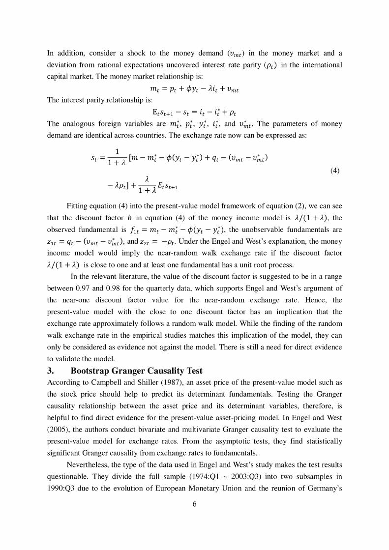
In addition, consider a shock to the money demand (/0�) in the money market and a

deviation from rational expectations uncovered interest rate parity (1�� in the international

capital market. The money market relationship is:

�� /0�

The interest parity relationship is:

E�� 1�

The analogous foreign variables are ��, ��, ��, ��, and /0�� . The parameters of money

demand are identical across countries. The exchange rate now can be expressed as:

�� 11 � � 2� � �� .� � �/0� � /0��

� �1�3 � �1 � � ��

(4)

Fitting equation (4) into the present-value model framework of equation (2), we can see

that the discount factor ' in equation (4) of the money income model is �/�1 � ��, the

observed fundamental is �� , the unobservable fundamentals are

(�� .� � �/0� � /0�� , and ()� � �14. Under the Engel and West’s explanation, the money

income model would imply the near-random walk exchange rate if the discount factor

�/�1 � �� is close to one and at least one fundamental has a unit root process.

In the relevant literature, the value of the discount factor is suggested to be in a range

between 0.97 and 0.98 for the quarterly data, which supports Engel and West’s argument of

the near-one discount factor value for the near-random exchange rate. Hence, the

present-value model with the close to one discount factor has an implication that the

exchange rate approximately follows a random walk model. While the finding of the random

walk exchange rate in the empirical studies matches this implication of the model, they can

only be considered as evidence not against the model. There is still a need for direct evidence

to validate the model.

3. Bootstrap Granger Causality Test

According to Campbell and Shiller (1987), an asset price of the present-value model such as

the stock price should help to predict its determinant fundamentals. Testing the Granger

causality relationship between the asset price and its determinant variables, therefore, is

helpful to find direct evidence for the present-value asset-pricing model. In Engel and West

(2005), the authors conduct bivariate and multivariate Granger causality test to evaluate the

present-value model for exchange rates. From the asymptotic tests, they find statistically

significant Granger causality from exchange rates to fundamentals.

Nevertheless, the type of the data used in Engel and West’s study makes the test results

questionable. They divide the full sample (1974:Q1 ~ 2003:Q3) into two subsamples in

1990:Q3 due to the evolution of European Monetary Union and the reunion of Germany’s

7

economy during this period, and use the full sample as well as the subsamples in the

asymptotic Granger causality test. Yet, conducting the asymptotic test with those subsamples

may lessen the creditability of the test result because the sample size of all subsamples is very

small. For example, the data of France, Germany and Italy all are not available after 1999:Q1,

and the number of observations in the later part of sample period (1990:Q3 ~ 2003:Q3) of

those countries is merely 34. It is known that the small-sample problem is very likely to occur

in this case, and we might need to find more evidence from other testing techniques such as

the bootstrap method to confirm the existing evidence for the model.

In response to the asymptotic Granger causality test in Engel and West’s (2005) paper,

the goal of this article is to re-assess the existing evidence of the present-value model for

exchange rates based on the bootstrap empirical distribution. The reason for choosing the

bootstrap method is that the bootstrap method is generally believed having less size distortion

and providing more precise test inferences than the asymptotic method in many applications

if the available sample size is small. Moreover, owing to advanced computer technology, the

bootstrapping technique now can be quickly implemented.

3.1 The VAR Model for the Granger Causality Test

In order to compare the new test results from the bootstrap test with the existing result from

the asymptotic test, the data used in this paper are identical to what Engel and West (2005)

used for their asymptotic Granger causality test. In addition, this paper focuses on the

bilateral relationship of the U.S. exchange rates against other six countries of G7 members.

The fundamental measures include the money supply fundamental �� , the output

fundamental (� � ��), the PPP fundamental (�� ), and the UIRP fundamental ( � � ��).

In addition, we also include the monetary fundamental. Following Mark (1995), the income

elasticity, , in the money demand is set to 1, so the monetary fundamental is �� . The exchange rate and each of the fundamental measures are shown to maintain

unit root processes, so they are presented in the first-differenced form. The data do not show

an explicit cointegration relationship between the exchange rate and each fundamental

measure, so the VAR model does not include a vector correction term.

The bivariate VAR model in testing the Granger causality relationship between Δ��

and Δ�� takes the form:

67��7��8 � 9:;:<= � � >?�� ?�)?)� ?))@ 67��A?7��A? 8 � 9B;,�B<,�=

D

?�� (5)

where :;and :< are the constant terms, and the innovation terms B;,� and B<,� are assumed

to be independently and identically distributed (i.i.d.) with mean zero and have variances EF,;)

and E<,;) , respectively. The null hypothesis of the Granger causality test between the

exchange rate and the fundamental restricts the parameters of �� or �� equation in model (5).

8

For example, the null hypothesis of the non-Granger causality running from the exchange rate

to the fundamentals restricts ?)�, � 1,…,4 to be zero.

3.2 Bootstrap Test Algorithm

Numerous bootstrap methods have been developed based on different properties of the time

series process (Li and Maddala, 1996, 1997; Berkowitz and Kilian, 2000). Because of the

simple algorithm in generating bootstrap replications, the residual-based bootstrap has

become the most popular one. Under the i.i.d. error assumption, one can repeatedly draw

residuals and generate the necessary pseudo data.

Since the Jarque-Bera test rejects the null hypothesis of the Gaussian innovation for

most of the data used in this paper, all bootstrap test inferences are drawn from the test with

nonparametric resampling method. The bootstrap algorithm for the Granger causality test

consists of four steps.

Step 1. Given the original observation, estimate coefficients by the estimated generalized

least square (EGLS) method for VAR model (5) under H₀ and H₁, respectively, and

obtain the test statistic �I.1 �I � J�KLMNOP M � KLMNOQM� (6)

NOP and NOQ are residual covariance matrices under R* and R�, respectively.

Step 2. Apply the estimates S?’s estimated under the null hypothesis in step 1 to generate the

pseudo-data {��, ��} with the same length as the original data {��, ��}. For instance,

if the null hypothesis is Δ�� does not Granger causes Δ��, the DGP is:

7�� :;̂ � � S?��7��A?�D

?�� S?�)7��A?�

D

?�� B;,��

7�� :<̂ � � S?))7��A?�D

?�� B<,��

(7)

To initialize this process, specify +Δ��A�� , Δ��A�� ,U � �0, 0�V for - � 1, … ,4 and

discard the first 500 created data. The pseudo innovation term B�� B;,�� , B<,�� V is

random and drawn with replacement from the set of observed residuals BY� ��BY;,�, BY<,��V obtained from step 1. After repeating this step 2000 times, the

1 Several standard test statistics, such as the F test statistic, the Wald statistic, and the likelihood ratio (LR) test

statistic, can be used in the bivariate Granger causality test. Since the standard F, Wald, and LR test statistics are

the same asymptotically, this paper provides the test result from the LR test statistic.

9

2000-bootstrapped samples are obtained. 2

Step 3. For each bootstrapped sample, re-estimate the coefficients in the VAR model (5), and

construct the corresponding test statistic �I� as in step 1.

�I� � J�KLMNOP� M � KLMNOQ

� M� (8)

Step 4. Use the 2000 test statistics �I� obtained from the bootstrapped replications in step 3

to construct the empirical distribution and determine the p-value for the LR statistic �I of step 1.

4. Empirical Results

Bootstrapping test results are determined by the empirical p-value from 2000 bootstrapped

samples, and the asymptotic test results are based on the p-value of the asymptotic Z)

distribution. Following Engel and West (2005), the full sample is divided into two

sub-samples in 1990:3 due to major economic and noneconomic developments in this period.

Tables 1 to 3 summarize p-values of the LR test statistics of the Granger causality test results

from different test methods on each sample period.3

Full Sample (1974:Q1~2001:Q3). Tables 1(a) and 1(b) summarize p-values of the LR

test statistic in Granger causality test from the full sample data based on the standard

asymptotic distribution and the empirical bootstrap distribution, respectively. Table 1(a)

shows that, at the 10% significant level, ten out of thirty null hypotheses that Δ�� fails to

Granger cause Δ�� based on the asymptotic distribution are rejected. There are no rejections

for Canada and the United Kingdom, and no null hypotheses are rejected in the cases of the

output fundamental Δ�� . At the 1% significance level, we reject the null hypothesis in

three out of six countries when we investigate the Granger causality relationship running

from the exchange rate to the PPP fundamental.The results based on the bootstrap Granger

causality test between the exchange rate and the fundamental are reported in Table 1(b). Table

1(b) shows seven rejections in thirty tests at the 10% significance level, so the evidence of the

causality running from the exchange rate to the fundamental is slightly weaker than what we

have seen in Table 1(a).

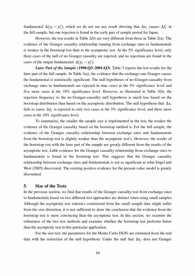
Early Part of the Sample (19974:Q1~1990:Q2). Table 2 summarizes the test results

for the early part of the full sample. As shown in Table 2(a), the asymptotic test result shows

more evidence that the exchange rate Granger causes the fundamental than the full sample. In

Table 2(a), the null that Δ�� fails to Granger cause Δ�� is rejected in ten cases at the 5%

significance level and in three more cases at the 10% significance level. For the output

2 This study refers to Davidson and MacKinnon (2000), choosing to bootstrap 2000 replications because the

bootstrapping p-value of the test statistic �I constructed from 2000 replications differed only marginally from

those constructed from 2500 or 5000 replications.

3 The asymptotic test in this paper is replication results of Engel and West’s Granger causality test.

10

fundamental Δ�� , which we do not see any result showing that Δ�� causes Δ�� in

the full sample, but one rejection is found in the early part of sample period for Japan.

However, the test results in Table 2(b) are very different from those in Table 2(a). The

evidence of the Granger causality relationship running from exchange rates to fundamentals

is weaker in the bootstrap test than in the asymptotic test. At the 5% significance level, only

three cases of the null of no Granger causality are rejected, and no rejections are found in the

cases of the output fundamental Δ�� .

Later Part of the Sample (1990:Q3~2001:Q3). Table 3 reports the test results for the

later part of the full sample. In Table 3(a), the evidence that the exchange rate Granger causes

the fundamental is statistically significant. The null hypotheses of no-Granger-causality from

exchange rates to fundamentals are rejected in nine cases at the 5% significance level and

five more cases at the 10% significance level. However, as illustrated in Table 3(b), the

rejection frequency to the no-Granger-causality null hypothesis is much less based on the

bootstrap distribution than based on the asymptotic distribution. The null hypothesis that Δ��

fails to cause Δ�� is rejected in only two cases at the 5% significance level, and three more

cases at the 10% significance level.

To summarize, the smaller the sample size is implemented in the test, the weaker the

evidence of the Granger causality based on the bootstrap method is. For the full sample, the

evidence of the Granger causality relationship between exchange rates and fundamentals

from the bootstrap test is slightly weaker than the asymptotic test’s. However, the results of

the bootstrap test with the later part of the sample are greatly different from the results of the

asymptotic test. Little evidence for the Granger causality relationship from exchange rates to

fundamentals is found in the bootstrap test. This suggests that the Granger causality

relationship between exchange rates and fundamentals is not as significant as what Engel and

West (2005) discovered. The existing positive evidence for the present-value model is greatly

discounted.

5. Size of the Tests

In the previous section, we find that results of the Granger causality test from exchange rates

to fundamentals based on two different test approaches are distinct when using small samples.

Although the asymptotic test statistics constructed from the small sample data might suffer

from the size distortion, it is not sufficient to draw the conclusion that the evidence from the

bootstrap test is more convincing than the asymptotic test. In this section, we examine the

robustness of the two test methods and examine whether the bootstrap test performs better

than the asymptotic test in this particular application.

For the size test, the parameters for the Monte Carlo DGPs are estimated from the real

data with the restriction of the null hypothesis. Under the null that Δ�� does not Granger

11

cause Δ��, the pseudo time-series sequence of +Δ��[, Δ��[,Uin a trial of the experiment is

generated by:

∆��[ � :;̂ � � S?��∆��A?[ � � S?�)∆��A?[ �D

?��

D

?��B;,�[

∆��[ � :<̂ � � S?))∆��A?[ � B<,�[D

?��

(9)

The regression coefficients :;̂, :<̂, S?��, S?�) and S?)), � 1, \ ,4, are estimated from the

observed data with the EGLS method. The innovation term in the Monte Carlo experiment

B�[ � �B;,�[ , �<,�[ �V is randomly drawn from the observed EGLS residuals. For each trial of the

Monte Carlo experiment, we use the parameter estimates to simulate the pseudo data for the

Granger causality test. Effective size of the asymptotic and the bootstrap test is determined by

the nominal 10% test with 1000 trials of the Monte Carlo experiment. For the bootstrap

Granger causality test, the algorithm is the same as illustrated in Section 3.

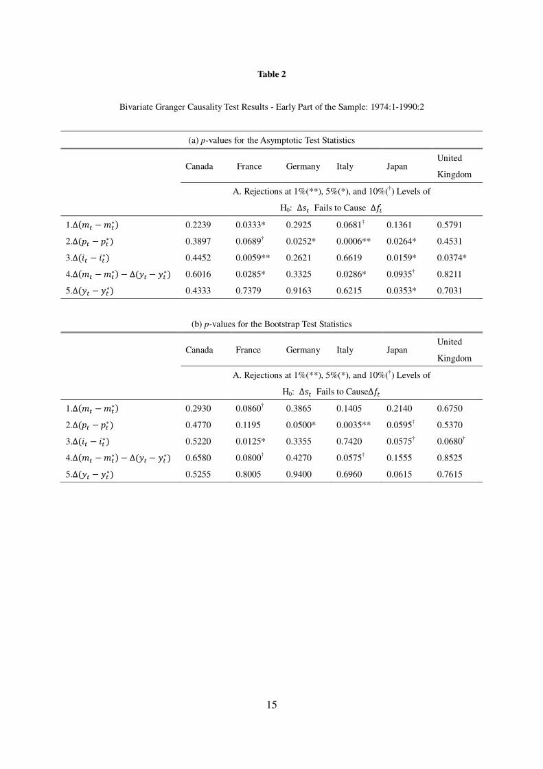
The size of the 10% test is tabulated in Figures 1 to 3. The numeric number of 1 to 6

represents Canada, France, Germany, Italy, Japan, and the United Kingdom, respectively. The

upper panel of the figures summarizes the size of the asymptotic tests, and the lower panel of

figures summarizes the size of the bootstrap tests. Since the nominal size of the test is 10%,

the ideal value of size of a test is 0.1. We see that, in the upper panel of Figure 1, the size of

the asymptotic test is slightly larger than 10%. For the early part of the sample, as the upper

panel of Figure 2 displays, size of the asymptotic test increases by a large percentage. For the

later part of the sample, the upper panel of Figure 3 shows that size of the asymptotic test

raises in all fundamental measures and in all sample countries by a large percentage.

Moreover, some magnitudes of the size of the asymptotic tests rise up to almost 40%.

In contrast, as what can be seen in the lower panels of Figure 1 to Figure 3, the size of

the bootstrap test does not change much and remains stable at the nominal 10% significance

level. Also, the size of the bootstrap test is lower than that of the asymptotic test in all

samples. The Monte Carlo study show that the asymptotic test has larger size distortion than

the bootstrap test in this particular application. It implies that the asymptotic Granger

causality test suffers the size distortion problem for the type of the data used in Engel and

West’s (2005) study, and there is a need to call for more direct evidence for the present-value

model for exchange rates.

12

6. Conclusion

This study is in response to the finding of the Granger causality relationship based on the

asymptotic test in Engel and West (2005). In Engel and West’s study, the authors use the

present-value model to explain the finding of the close to random walk exchange rate in

empirical studies. Although the empirical findings of the near-random walk exchange rate are

consistent with the exchange rate behavior under their explanation, the findings are not

sufficient to directly confirm the present-value model for exchange rates. The Granger

causality test with the asymptotic method is implemented to validate the model. However, the

type of data used in their study is very likely to lead to the size distortion in the test results

because the sample size of the data is small.

This paper employs the bootstrap method to re-evaluate the evidence of the causality

relationship between exchange rates and fundamentals. The bootstrap test results show that

the evidence of Granger causality from exchange rates to fundamentals is not as significant as

the existing evidence from the asymptotic method in all sample periods. Additionally, the

Monte Carlo experiment results demonstrate that the bootstrap test performs better than the

asymptotic test in respect of the robustness of the tests in this particular application. The large

size in the asymptotic test shows that Engel and West’s results are greatly distorted by the

small-sample problem. Therefore, the existing Granger causality evidence is not strong

enough to support the present-value model for exchange rate under Engel and West’s

explanation.

More direct evidence is needed for the present-value model for exchange rates. One

may explore long-horizon exchange rate predictability under the present-value model. For

example, over the longer horizon, the near-one discount rate factor becomes smaller, so one

of Engel and West’s assumptions for the near random walk exchange rate fails. We might find

exchange rate predictability over the long horizon. Also, if the unobservable fundamentals are

not I(1), the long-horizon regression may have predictability power for exchange rate (Engel

Wang, and Wu, 2010).

References

Andrews, Donald W. K. and Moshe Buchinsky. 2000. “A Three-step Method for Choosing the Number of

Bootstrap Repetitions.” Econometrica 68 (1): 23-51.

Ashley, Richard, Clive W. J. Granger , and Richard Schmalensee. 1980. “Advertising and Aggregate

Consumption: An Analysis of Causality.” Econometrica 48 (5): 1149-67.

Berkowitz, Jeremy and Lutz Kilian. 2000. “Recent Developments in Bootstrapping Time Series.” Econometric

Reviews 19 (1): 1-48.

Campbell, John Y. Campbell and Robert J. Shiller. 1987. “Cointegration and Tests of Present Value Models.”

The Journal of Political Economy 95 (5): 1062-88.

Cheung, Yin-Wong, Menzie D. Chinn and Antonio G. Pascual. 2005. “Empirical Exchange Rate Models of the

13

Nineties: Are Any Fit to Survive?” Journal of International Money and Finance 24 (7): 1150-75.

Davidson, Russell and James G. MacKinnon. 2000. “Bootstrap Tests: How Many Bootstraps?” Econometric

Reviews 19 (1): 55-68.

Efron, Bradley and Robert Tibshirani. 1993. An Introduction to the Bootstrap. New York, NY, Chapman &

Hall.

Engel, Charles, Jian Wang and Jason Wu. 2010. “Long-Horizon Forecasts of Asset Prices when the Discount

Rate is Close to Unity.” Working paper, University of Wisconsin, Madison.

Engel, Charles and Kenneth D. West. 2005. “Exchange Rate and Fundamentals.” Journal of Political Economy

113 (3): 485-517.

Faust, Jon, John H. Rogers, and Jonathan H. Wright. 2003. “Exchange Rate Forecasting: the Errors We've

Really Made.” Journal of International Economics 60 (1): 35-59.

Frenkel, Jacob A. 1976. “A Monetary Approach to the Exchange Rate: Doctrinal Aspects and Empirical

Evidence.” Scandinavian Journal of Economics 78 (2): 200-24.

______. 1979. “On the Mark: A Theory of Floating Exchange Rates Based on Real Interest Differentials.” The

American Economic Review 69 (4): 610-22.

Granger, Clive W. J. 1969. “Investigating Causal Relations by Econometric Models and Cross-spectral

Methods.” Econometrica 37 (3): 424-38.

Peter Hall. (1986). “On the Number of Bootstrap Simulations Required to Construct a Confidence Interval.” The

Annals of Statistics 14 (4): 1453-62.

Kilian, Lutz. 1999. “Exchange Rates and Monetary Fundamentals: What Do We Learn from Long-Horizon

Regressions?” Journal of Applied Econometrics 14 (5): 491-510.

Li, G. S. Hongyi and Maddala. 1996. “Bootstrapping Time Series Models.” Econometric Reviews 15 (2):

115-58.

______. 1997. “Bootstrapping Cointegrating Regressions.” Journal of Econometrics 80 (2): 297-18.

Ma, Yue and Angelos Kanas. 2000. “Testing for Nonlinear Granger Causality from Fundamentals to Exchange

Rates in the ERM.” Journal of International Financial Markets, Institutions and Money 10 (1): 69-82.

_______. 2000. “Testing for a nonlinear relationship among fundamentals and exchange rates in the ERM”

Journal of International Money and Finance 19 (1): 135-52

Mark, Nelson C. 1995. “Exchange Rates and Fundamentals: Evidence on Long-Horizon Predictability.” The

American Economic Review 85 (1): 201-18.

Mark, Nelson C. and Donggyu Sul. 2001. “Nominal exchange rates and monetary fundamentals: Evidence from

a small post-Bretton woods panel.” Journal of International Economics 53 (1): 29-52.

Meese, Richard A., and Kenneth Rogoff. 1983a. “Empirical Exchange Rate Models of the Seventies: Do They

Fit Out of Sample?” Journal of International Economics 14 (1-2): 3-24.

_______. 1983b. “The Out of Sample Failure of Empirical Exchange Rate Models” in Jacob A. Frenkel, ed.,

Exchange Rates and International Macroeconomics. Chicago, IL: University of Chicago Press, pp. 6-105

Obstfeld, Maurice, and Kenneth Rogoff. 2000. “The Six Major Puzzles in International Macroeconomics: Is

There a Common Cause?” NBER Macroeconomics Annual 15, 339-90.

14

Table 1

Bivariate Granger Causality Test Results- Full Sample: 1974:1-2001:3

(a) p-values for the Asymptotic Test Statistics

Canada France Germany Italy Japan United

Kingdom

A. Rejections at 1%(**), 5%(*), and 10%(†) Levels of

H0: Δ�� Fails to Cause Δ��

1.Δ�� 0.1660 0.0668† 0.6117 0.0367* 0.0177* 0.3544

2.Δ�� 0.9324 0.1118 0.0079** 0.0023** 0.0092** 0.5522

3.Δ� � � �� 0.3834 0.0156* 0.2674 0.5608 0.0019** 0.1165

4. Δ�� Δ�� 0.2287 0.0775† 0.7873 0.0587† 0.1155 0.4876

5.Δ�� 0.1125 0.6602 0.9628 0.7882 0.6698 0.5153

(b) p-values for the Bootstrap Test Statistics


Kingdom



1.Δ�� 0.1915 0.1110 0.6665 0.0605† 0.0360* 0.3965

2.Δ�� 0.9350 0.1530 0.0150* 0.0040** 0.0145* 0.5960

3.Δ� � � �� 0.4115 0.0235* 0.3230 0.6080 0.0045** 0.1595

4. Δ�� Δ�� 0.2610 0.1280 0.8275 0.0940† 0.1625 0.5365

5.Δ�� 0.1420 0.7050 0.9675 0.8215 0.7120 0.5745

15

Table 2

Bivariate Granger Causality Test Results - Early Part of the Sample: 1974:1-1990:2



Kingdom



1.Δ�� 0.2239 0.0333* 0.2925 0.0681† 0.1361 0.5791

2.Δ�� 0.3897 0.0689† 0.0252* 0.0006** 0.0264* 0.4531

3.Δ� � � �� 0.4452 0.0059** 0.2621 0.6619 0.0159* 0.0374*

4.Δ�� Δ�� 0.6016 0.0285* 0.3325 0.0286* 0.0935† 0.8211

5.Δ�� 0.4333 0.7379 0.9163 0.6215 0.0353* 0.7031



Kingdom


H0: Δ�� Fails to CauseΔ��

1.Δ�� 0.2930 0.0860† 0.3865 0.1405 0.2140 0.6750

2.Δ�� 0.4770 0.1195 0.0500* 0.0035** 0.0595† 0.5370

3.Δ� � � �� 0.5220 0.0125* 0.3355 0.7420 0.0575† 0.0680†

4.Δ�� Δ�� 0.6580 0.0800† 0.4270 0.0575† 0.1555 0.8525

5.Δ�� 0.5255 0.8005 0.9400 0.6960 0.0615 0.7615

16

Table 3

Bivariate Granger Causality Test Results - Later Part of the Sample: 1990:3-2001:3



Kingdom



1.Δ�� 0.0226* 0.0627† 0.8818 0.3189 0.0344* 0.2139

2.Δ�� 0.0583† 0.0172* 0.0001** 0.1646 0.3490 0.0988†

3.Δ� � � �� 0.1646 0.5221 0.0462* 0.0453* 0.0627† 0.5340

4.Δ�� Δ�� 0.0039** 0.0202* 0.4830 0.6224 0.5327 0.0546†

5.Δ�� 0.1094 0.2003 0.6515 0.2781 0.3139 0.0217*



Kingdom



1.Δ�� 0.0745† 0.2145 0.9420 0.5620 0.1120 0.3630

2.Δ�� 0.1685 0.0705† 0.0025** 0.2855 0.5175 0.2095

3.Δ� � � �� 0.3105 0.6940 0.1365 0.1165 0.1675 0.6640

4.Δ�� Δ�� 0.0245* 0.1205 0.7100 0.7835 0.6780 0.1345

5.Δ�y4 � y4�� 0.2310 0.3605 0.7620 0.4305 0.4880 0.0665†

17

Figure 1

Size of the Test- Full Sample (1974:1-2001:3)

NOTE.— Number 1 to 6 represents Canada, France, Germany, Italy, Japan, and the United Kingdom,

respectively. The upper panel and lower panel of the figures summarizes the size of the asymptotic Granger

causality tests and that of the bootstrap Granger causality tests from exchange rates to fundamentals,

respectively.

18

Figure 2

Size of the Test- Early Part of the Sample (1974:1-1990:2)

NOTE.— Same as the note of Figure 1.

19

Figure 3

Size of the Test- Later Part of the Sample (1990:3-2001:3)

NOTE.—Same as the note of Figure 1.

bootstrap granger causality revising - teaweb.org.t · present-value model is also determined by a...

Documents