bond price representations and the volatility of spot interest rates

Review of Quantitative Finance and Accounting, 7 (1996): 279-288 © 1996 Kluwer Academic Publishers, Boston. Manufactured in The Netherlands.

Bond Price Representations and the Volatility of Spot Interest Rates

PETER RITCHKEN Weatherhead School of Management, Case Western Reserve University, Cleveland, OH 44106

L. SANKARASUBRAMANIAN EA.S.T., Bear Sterns, 245 Park Avenue, New York, NY 10167

Abs t rac t

A common approach to modeling the term structure of interest rates in a single-factor economy is to assume that the evolution of all bond prices can be described by the current level of the spot interest rate. This article inves- tigates the restrictions that this assumption imposes. Specifically, we show that this Markovian restriction, together with the no-arbitrage requirement, curtails the relationship of forward rates and their volatilities relative to spot-rate volatilities. Among such Markovian models, only a few provide simple analytical relationships between bond prices and the spot interest rate. This article identifies the class of spot-rate volatility specifications that permit simple analytical linkages to be derived between bond prices and interest rates. Included in the class are the volatility structures used by Vasicek and by Cox, Ingersoll, and Ross. Surprisingly, no other volatility structures permit simple analytical representations.

Key words: bond pricing, Markou moders, analytical solutions

1. Introduction

Models of the term structure usually assume that the evolution of all bond prices is determined by one or more factors of uncertainty. In most models the number of "state vari-

ables" required to describe the entire term structure at any point in time is assumed to equal the number of factors generating uncertainty. For example, almost all single-factor

models derive or assume the instantaneous spot rate to be the single-state variable. In two- factor models a second "state variable," such as the long rate or the rate of inflation is added. Of course, in general, the number of state variables need not equal the number of factors. For example, in the general single-factor models of Heath, Jarrow, and Morton (HJM) (1992), the evolution of the term structure cannot be characterized by a finite num-

ber of state variables and is influenced by the entire history of the process. It follows then that in order to model the term structure by a process that is Markovian with respect to a

finite-state space, specific assumptions need to be made either explicitly or implicitly. In this article we identify the constraints that must be imposed on a single-factor model to ensure that the evolution of the term structure can be characterized by the spot rate alone, without regard to the history of the process. We show that the Markovian requirement imposes specific restrictions on the forward-rate curve.

Among the class of single-factor Markovian models, only a few cases have been identified where simple analytical relationships exist between forward rates of all maturities and

280 p. RITCHKEN AND E SANKARASUBRAMANIAN

the spot rate. Examples are the Vasicek (1977) model, where spot-rate variances are deterministic, and the Cox, Ingersoll, and Ross (CIR) (1985) model, where spot-rate variances are proportional to the level of the spot rate. For other specifications of the spot-rate volatility, simple analytical representations of the term structure have been lacking. This raises the question as to the nature of the class of volatility structures that give rise to simple analytical linkages between interest rates and bond prices. This article identifies the class of volatilities in a single-factor economy that permit simple analytical models to be developed.

2. The non-Markovian nature of bond prices in a single-factor model

In this section, we review the fundamental relationships that any viable model of the term structure must satisfy when uncertainty is described by an Ito process. First, let P(t, 7) be the price at date t of a pure discount bond that matures at time T. By definition, the bond price can be expressed as

T P (t,7) = e - f t f(t,s)ds. (1)

Heref(t , s) is the forward interest rate, viewed from time t, for the time increment [s, s + ds]. Most single-factor models either explicitly or implicitly assume that bond prices and forward rates evolve according to

d f (t,T) = #f( t ,7)dt + o'f(t,7)dw(t), for T > t, (2a)

and

dP (t, 7) (2b) P (t, 7) - #p(t,T)dt + Crp(t,7)dw(t), for T > t.

In general, these drift and volatility terms could depend on the entire information set at date t. However, as Heath, Jarrow, and Morton (1992) demonstrate, to avoid dynamic arbitrage opportunities across bond of all maturities, the following relations must be satisfied:

#f(t ,7) = crf(t,7)[)~(t) - ~rp(t,7)] (3a)

Crp(t,7) = - f ~ of(t, u)du (3b)

#p(t,7) = r (t) + )~(t)o'p(t,7). (3c)

Here )~(t) is the market price of interest-rate risk at time t and is perhaps stochastic but is the same for all bonds regardless of maturity. 1 Substituting from equations (3a) to (3c) into equations (2a) to (2b) and integrating leads to the intertemporal relationships for forward rates and bond prices:

BOND PRICE REPRESENTATIONS AND SPOT INTEREST RATES 281

and

L/~0,t) j

Equations (4a) and (4b) show that the setting of the term structure at date t depends on the setting at an earlier date 0, together with all the Brownian disturbances and the evolution of the market price of risk over the entire time period [0,t]. Hence, unless additional structure is placed on the volatilities of all forward rates, crj(u,T), we cannot, in general, identify a finite set of state variables that characterize the term structure.

3. Single-state, single-factor Markovian models of the term structure

Most arbitrage-free models of bond prices and interest-rate claims avoid the path-dependence problem by explicitly or implicitly assuming that all forward rates (and bond prices) depend on a single-state variable. For example, a common approach is to take the short interest rate as the relevant state variable and to specify its dynamics directly. A key distin- guishing feature of most single-state models of the term structure concerns the assumptions placed on the evolution of the spot interest rate. In many models, the instantaneous variance of the spot interest rate, cr2(r,t), is assumed to have constant elasticity and to be of the form 2

~2(r,0 = o-2[r(O]~. (5)

Given the spot-rate dynamics, arbitrage arguments alone, together with an appropriate specification for the market price of interest-rate risk, lead to the identification of forward interest rates and bond prices. Further, since forward interest rates depend on the spot interest rate alone, their volatilities are given by

o)(t,T) = f~(t,7)~r(r,t). (6)

Hence the volatilities of all forward interest rates are determined by the specification of the volatility of the spot interest rate and the functional relationship between spot and forward interest rates. In only a few cases, however, have simple analytical linkages between forward interest rates and the spot interest rate been established. In the cases where simple analytical solutions exist (Vasicek and CIR), forward rates are linear in the spot rate and equations (4a) and (4b) reduce to the form

P(t,7) = e c'{t'r)-p(t,r>(O (7a)

and

f (t,T) = -o:r( t ,T ) + flr(t,T)r(O, (7b)

282 P. RITCHKEN AND E SANKARASUBRAMANIAN

where GUY) and/3(t,T) are independent oft(t), and the subscripts denote derivatives. In fact, for the Vasicek and CIR models, forward-rate variances are deterministic and linear in the spot rate, respectively. To date, no analytic representations of forward rates and their volatilities have been identified for any spot-rate variance specifications other than those consid- ered by Vasicek and CIR. 3 This raises the question of whether other spot-rate volatility specifications are likely to lead to simple analytical forms. To answer this question, however, we first need to identify the constraints that the single-state Markovian restriction imposes between forward rates and spot-rate volatilities. Lemma 1 below addresses this issue.

L e m m a 1. When interest rates follow an Ito process, the requirement that all bonds be priced off a common single state variable restricts the forward-rate curve as

L( t , r ) • [fr(t,r)lr=,] + f,(t,:r) 1 ~,2(r,0, 2f,(t,r) f ; fr(t,x)dx - f , r ( t , r ) =

where the subscripts denote partial derivatives in the usual sense.

(8)

Proof See Appendix 1.

The left side of equation (8) is completely determined by the functional representation of forward rates and does not contain either the drift of the spot interest rate or the market price of risk. The equation highlights the fact that forward rates and their volatilities are largely determined by the choice of the volatility of the spot interest rate. 4

Let g(r) be any twice differentiable function of the spot rate, r(t). Further, assume that all forward rates can be expressed as polynomials of arbitrary order n in g(r). In other words,

f(t,T) = 2 a~(t,T)[g(r)]/~, for all T > t, (9) k=0

where an(t, T) ~ O. Clearly, if g(r) = r, then forward rates can be expressed as a polynomial in the spot rate. The following theorem uses the lemma to identify the conditions on volatilities that permits forward rates to be represented in terms of this polynomial.

T h e o r e m 1. I f interest rates follow a single-state Ito process, then, for forward interest rates to be represented by a finite degree polynomial in the spot interest rate, the volatility of spot interest rate must be restricted to the class

o'2(r,O = bo(O + bl(Or (0, (10)

where bo(t ) and bl(t ) are independent of the level of the term structure.

Proof See Appendix 1.

The theorem shows that for forward interest rates to have a form similar to equation (7b), the variances of spot rates must be linear in the spot rate. Notice that while the


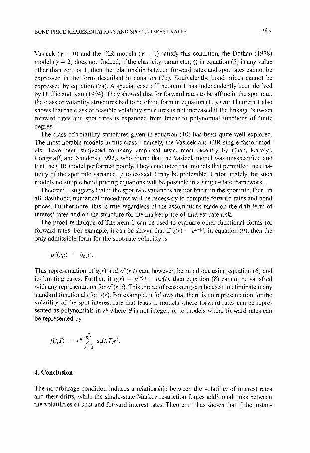
Vasicek O' = 0) and the CIR models (~' = 1) satisfy this condition, the Dothan (1978) model (~/= 2) does not. Indeed, if the elasticity parameter, ~, in equation (5) is any value other than zero or 1, then the relationship between forward rates and spot rates cannot be expressed in the form described in equation (7b). Equivalently, bond prices cannot be expressed by equation (7a). A special case of Theorem 1 has independently been derived by Duffle and Kan (1994). They showed that for forward rates to be affine in the spot rate, the class of volatility structures had to be of the form in equation (10). Our Theorem 1 also shows that the class of feasible volatility structures is not increased if the linkage between forward rates and spot rates is expanded from linear to polynomial functions of finite degree.

The class of volatility structures given in equation (10) has been quite well explored. The most notable' models in this class--namely, the Vasicek and CIR single-factor mod- e l s -have been subjected to many empirical tests, most recently by Chart, Karolyi, Longstaff, and Sanders (1992), who found that the Vasicek model was misspecified and that the CIR model performed poorly. They concluded that models that permitted the elasticity of the spot rate variance, ?; to exceed 2 may be preferable. Unfortunately, for such models no simple bond pricing equations will be possible in a single-state framework.

Theorem 1 suggests that if the spot-rate variances are not linear in the spot rate, then, in all likelihood, numerical procedures will be necessary to compute forward rates and bond prices. Furthermore, this is true regardless of the assumptions made on the drift term of interest rates and on the structure for the market price of interest-rate risk.

The proof technique of Theorem 1 can be used to evaluate other functional forms for forward rates. For example, it can be shown that ifg(r) = e~r(0, in equation (9), then the only admissible form for the spot-rate volatility is

o-2(r,t) = b0(0.

This representation ofg(r) and o-2(r,t) can, however, be ruled out using equation (6) and its limiting cases. Further, if g(r ) = ear(O + mr(t) , then equation (8) cannot be satisfied with any representation for ~r2(r, t). This thread of reasoning can be used to eliminate many standard functionals for g(r) . For example, it follows that there is no representation for the volatility of the spot interest rate that leads to models where forward rates can be represented as polynomials in r o where 0 is not integer, or to models where forward rates can be represented by

f ( t , r ) = r0 ~ , ak(t,r)rk. k=0

4. Conclusion

The no-arbitrage condition induces a relationship between the volatility of interest rates and their drifts, while the single-state Markov restriction forges additional links between the volatilities of spot and forward interest rates. Theorem 1 has shown that if the instan-


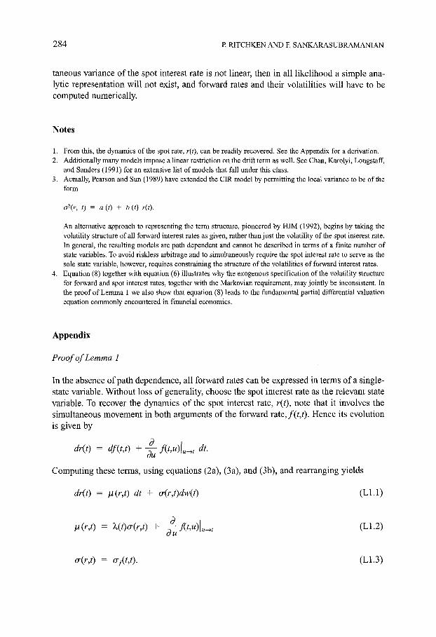
taneous variance of the spot interest rate is not linear, then in all likelihood a simple analytic representation will not exist, and forward rates and their volatilities will have to be computed numerically.

Notes

1. From this, the dynamics of the spot rate, r( t ) , can be readily recovered. See the Appendix for a derivation. 2. Additionally many models impose a linear restriction on the drift term as well. See Chan, Karolyi, Longstaff,

and Sanders (1991) for an extensive list of models that fall under this class. 3. Actually, Pearson and Sun (1989) have extended the CIR model by permitting the local variance to be of the

form

~r2(r, t) = a (t) + b ( t) r( t ) .

An alternative approach to representing the term structure, pioneered by HJM (1992), begins by taking the volatility structure of all forward interest rates as given, rather than just the volatility of the spot interest rate. In general, the resulting models are path dependent and cannot be described in terms of a finite number of state variables. To avoid riskless arbitrage and to simultaneously require the spot interest rate to serve as the sole state variable, however, requires constraining the structure of the volatilities of forward interest rates.

4. Equation (8) together with equation (6) illustrates why the exogenous specification of the volatility structure for forward and spot interest rates, together with the Markovian requirement, may jointly be inconsistent. In the proof of Lemma 1 we also show that equation (8) leads to the fundamental partial differential valuation equation commonly encountered in financial economics.

Appendix

Proof o f Lemma 1

In the absence of path dependence, all forward rates can be expressed in terms of a single- state variable. Without loss of generality, choose the spot interest rate as the relevant state variable. To recover the dynamics of the spot interest rate, r(t), note that it involves the simultaneous movement in both arguments of the forward rate, f(t,t). Hence its evolution is given by

dr(t) = df(t,t) + - ~ f(t,u)[u~, dt.

Computing these terms, using equations (2a), (3a), and (3b), and rearranging yields

dr(t) = #(r,t) dt + ~r(r,t)dw(t) (LI.1)

3 ~(r,t) = )~(t)~(r,t) + ~--flt ,u)]u~ t (L1.2)

d u "

~r(r,t) = o-fit, t). (L1.3)


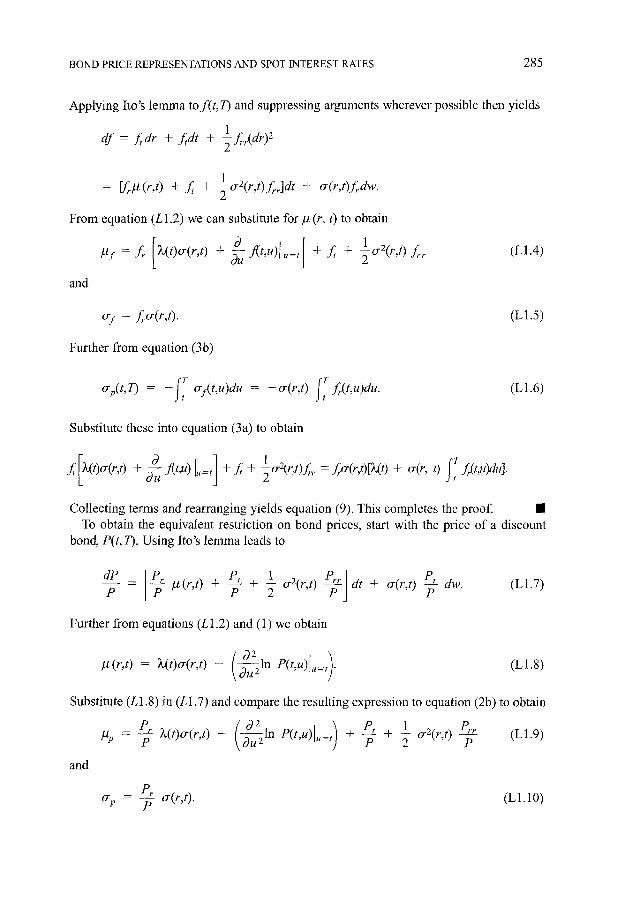
Applying Ito's lemma tof(t,T) and suppressing arguments wherever possible then yields

df = frdr + f d t + l f . r(dr)2

= [frCl(r,t) + f + lo-2(r,t)frr]dt + o-(r,t) frdw.

From equation (L1.2) we can substitute for/1 (r, t) to obtain

[ j 1 11f = f~ )~(t)o'(r,t) + ~ flt, u)l ,=t + f + °2(r,O f~r (L1.4)

and

0 7 = L ~ ( r , 0 . (L1.5)

Further from equation (3b)

O-p(t,7) = - t o'f(t,u)du = -o'(r,t) tr f~(t'u)du" (L1.6)

Substitute these into equation (3a) to obtain

f t)o-(r,t) + fit, u) I,=t + f + 3 °" (r,t)f,r = f°'(r,t)Dv(t) + o-(r, t) f t f(t,u)du].

Collecting terms and rearranging yields equation (9). This completes the proof. • To obtain the equivalent restriction on bond prices, start with the price of a discount

bond, P(t, 7). Using Ito's lemma leads to

p = 11(r,t) + P~P + 12 °-2(r't) dt + cr(r,t) --fi- dw. (El.7)

Further from equations (L1.2) and (1) we obtain

y(r,t) = £(t)o-(r,O - ~u21n P(t,u)[,= t . (L1.8)

Substitute (L 1.8) in (L 1.7) and compare the resulting expression to equation (2b) to obtain

Pr )~(Oo'(r,t) - ( 02 ) - - ~/P = T ~ U 21n P(/'b/)l + at + L o-2(r,t) /grr (El.9) u=t P 2 P

and

Pr o-(r,t). (L 1.10) % = T


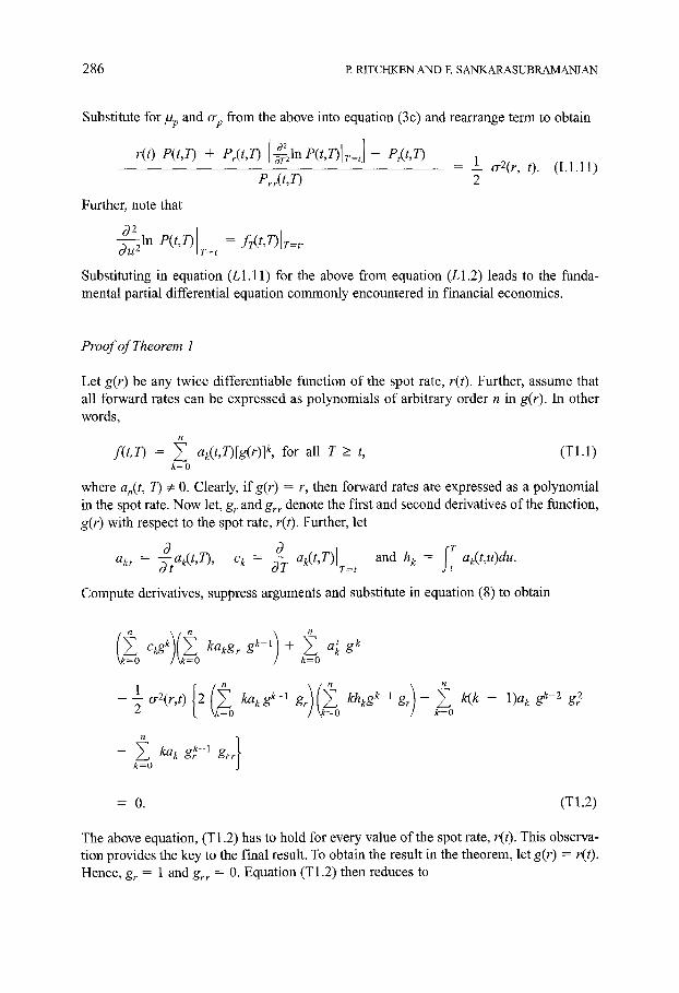
Substitute for #p and crp from the above into equation (3c) and rearrange term to obtain

r(t) P(t,T) + ~2

rr(t,T) [~r-?nP(t,T)lr=,]- P,(t,T) = 1 o_2(r, t). (LI . l l ) Pr~(t,T) 2

Further, note that

02 o~uzln P(t,T) r=t = fz(t'T)]r=r

Substituting in equation (LI.11) for the above from equation (L1.2) leads to the fundamental partial differential equation commonly encountered in financial economics.

Proof o f Theorem 1

Let g(r) be any twice differentiable function of the spot rate, r(t). Further, assume that all forward rates can be expressed as polynomials of arbitrary order n in g(r). In other words,

f(t ,T) = 2 ak(t,T)[g(r)]k, for all T > t, (TI.1) k=0

where an(t, 7) ~ O. Clearly, if g(r) = r, then forward rates are expressed as a polynomial in the spot rate. Now let, g~ and gr~ denote the first and second derivatives of the function, g(r) with respect to the spot rate, r(t). Further, let

3 0 and h k = f~ ak(t,u)du. a~ , = -~a~(t,T), ok = ~ ak(t,T)lr= '

Compute derivatives, suppress arguments and substitute in equation (8) to obtain

ckgk kakg ~ gk-1 + a~ gk k=0

2 k=O k(k - 1)a k gk-2 gr 2

- k=02 kak g)-I grr]

= 0 . ( T 1 . 2 )

The above equation, (T1.2) has to hold for every value of the spot rate, r(t). This observa- tion provides the key to the final result. To obtain the result in the theorem, let g(r) = r(t). Hence, gr = 1 and grr = 0. Equation (T1.2) then reduces to


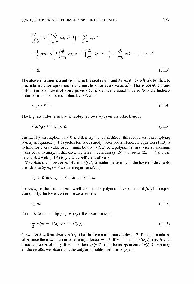
(k=~O ckrk) (~=~0 kak rk-1) + ~-o a~rk

k(k - 1)akrk-2

= 0. ( 7 1 . 3 )

The above equation is a polynomial in the spot rate, r and its volatility; cr2(r,t). Further, to preclude arbitrage opportunities, it must hold for every value of r. This is possible if and only if the coefficient o f every power of r is identically equal to zero. Now the highest- order term that is not multiplied by o2(r,t) is

ncnanr2"-l. (T1.4)

The highest-order term that is multiplied by o4(r,O on the other hand is

n2anhn(r 2n-2 o'2(r,t)). (T1.5)

Further, by assumption a , ~ 0 and thus h, ¢ 0. In addition, the second term multiplying o-2(r,t) in equation (T 1.3) yields terms of strictly lower order. Hence, if equation (T 1.3) is to hold for every value of r, it must be that cr2(r,t) be a polynomial in r with a maximum order equal to unity. In that case, the term in equation (T1.5) is o f order (2n - 1) and can be coupled with (T1.4) to yield a coefficient o f zero.

To obtain the lowest order of r in o-2(r,t), consider the term with the lowest order. To do this, denote by m, (m < n), an integer satisfying

a m ~ 0 and a k = 0, for all k < m.

Hence, a n is the first nonzero coefficient in the polynomial expansion off(t ,T). In equation (T1.3), the lowest order nonzero term is

Cmrm. (T1.6)

From the terms multiplying o-2(r,t), the lowest order is

1 m(m - 1)a m r m-2 o-2(r,t). (Yl.7)

Now, if m > 2, then clearly o-2(r, t) has to have a minimum order of 2. This is not admissible since the maximum order is unity. Hence, m < 2. I f m = 1, then o-2(r, t) must have a minimum order of unity. I f m = 0, then o-2(r, t) could be independent o f r(t). Combining all the results, we obtain that the only admissible form for ~2(r, t) is


~r2(r,t) = bo(t ) + bl(t ) r(t).

This completes the proof.

References

Chan, K. C., G. Karolyi, E Longstaff, and A. Sanders, "An Empirical Comparison of Alternative Models of the Term Structure of Interest Rates," Journal of Finance 47, 1209-1228, (1992).

Cox, L, J. Ingersoll, and S. Ross, "A Theory of the Term Structure of Interest Rates," Econometrica 53(2), 385-467, (1985).

Dothan, U. L. "On the Term Structure of Interest Rates," Journal of Financial Economics 4, 59-69, (1978). Duffle, D., and R. Kan, "A Yield Factor Model of Interest Rates," Working paper, Graduate School of Business,

Stanford University, 1994. Heath, D., R. Jarrow, and A. Morton, "Bond Pricing and the Term Structure of Interest Rates: A New

Methodology for Contingent Claims Valuation," Econometrica 60, 77-105, (1992). Pearson, N. D., and T. S. Sun, "A Test of the Cox, Ingersoll and Ross Model of the Term Structure of Interest

Rates Using the Method of Maximum Likelihood," Working paper, Sloan School, MIT, 1989. Vasicek, O., "An Equilibrium Characterization of the Term Structure," Journal of Financial Economics,

177-188, (November 1977).

bond price representations and the volatility of spot interest rates

Documents