boeing 757-200 interior simulation for cabin air quality ... · boeing 757-200 interior simulation...

Boeing 757-200 Interior Simulation for CabinAir Quality Analysis

Sigurður Ingi Einarsson

Thesis of 30 ECTS creditsMaster of Science (M.Sc.) in Mechanical Engineering

June 2015

Boeing 757-200 Interior Simulation for Cabin Air QualityAnalysis

Thesis of 30 ECTS credits submitted to the School of Science and Engineeringat Reykjavík University in partial fulfillment of

the requirements for the degree ofMaster of Science (M.Sc.) in Mechanical Engineering

June 2015

Supervisors:

Joseph Timothy Foley, SupervisorProfessor, Reykjavík University, Iceland

Þorgeir Pálsson, SupervisorProfessor Emeritus, Reykjavík University, Iceland

Examiners:

Páll Valdimarsson, ExaminerAdjunct Professor, Reykjavík University, Iceland

CopyrightSigurður Ingi Einarsson

June 2015

Boeing 757-200 Interior Simulation for Cabin Air QualityAnalysis


Thesis of 30 ECTS credits submitted to the School of Science and Engineeringat Reykjavík University in partial fulfillment of

the requirements for the degree ofMaster of Science (M.Sc.) in Mechanical Engineering

June 2015

Student:


Supervisors:

Joseph Timothy Foley

Þorgeir Pálsson

Examiner:

Páll Valdimarsson

The undersigned hereby grants permission to the Reykjavík University Library to reproducesingle copies of this Thesis entitled Boeing 757-200 Interior Simulation for Cabin AirQuality Analysis and to lend or sell such copies for private, scholarly or scientific researchpurposes only.

The author reserves all other publication and other rights in association with the copyrightin the Thesis, and except as herein before provided, neither the Thesis nor any substantialportion thereof may be printed or otherwise reproduced in any material form whatsoeverwithout the author’s prior written permission.

date

Sigurður Ingi EinarssonMaster of Science

Boeing 757-200 Interior Simulation for Cabin AirQuality Analysis


June 2015

Abstract

With increased competition in the flight industry Icelandair has heightened theirfocus on the well being of their passengers even more as well as upgrading boththe seats and the entertainment system on board most if not all of their aircraft.A few complaints have been lodged regarding the temperature in the cabin fromboth passengers as well as the crew. In order for Icelandair to maintain theircompetitive edge it is important for them to discover whether these complaints arebased in fact, and if there are some reasonable solutions present to improve theoverall passenger comfort during flight.

This thesis explores whether there is a way to establish a baseline for the airconditioning system so that a standardized measurement test could be carriedout in an arbitrary aircraft, would show if said aircraft system is functioning asintended compared to a baseline model.

To this end measurements were carried out on board an empty aircraft in Keflavikairport. To establish a baseline the decision was made to model the aircraft usingthe 3D Computer Aided Design (CAD) program Autodesk Inventor Professional(AIP) and import that model into Autodesk Simulation CFD (ASCFD) to simu-late the measured data. First the whole passenger cabin was simulated but laterit was decided to build a smaller surrogate for optimization of the cabin due tohigh element count and thus a long solution time. The results from the large simu-lated passenger cabin does however suggest that there are no dead spots or stagnantair pockets present in the cabin. The smaller surrogate of the aircraft called “TheSlice” included three seat rows. To compare the measured data to the simulationsMatlab was used to estimate the transfer functions of both the measured and thesimulated data from a set of seven time periods resulting from the measurements.The systems were then plotted for comparison. The starting temperature of eachperiod was used as a starting point in the corresponding simulation. To compareeach time period to its corresponding simulation the step response of both the mea-sured and simulated time periods were plotted. The overlaid plots show that thesimulations are well grounded to the measured data. To establish a baseline doeshowever require more measurements than from only one plane as was the casein this thesis. The results do however suggest that it would be feasible to modelsuch a baseline for a simple way to determine if the air conditioning system onboard some randomly selected aircraft is functioning as intended compared to thebaseline model.

xii

Hermun á lofteiginleikum í farþegarými Boeing757-200 flugvéla


júní 2015

Útdráttur

Með aukinni samkeppni í flugiðnaði hefur Icelandair beint sjónum sínum ennfrekar að velferð farþega sinna auk þess sem þeir hafa uppfært bæði sætin semog afþreyingarkerfin í flestum ef ekki öllum vélunum sínum. Þrátt fyrir það hafakvartanir borist frá bæði farþegum sem og áhöfn vegna hita í farþegarými á meðaná flugi stendur. Til að Icelandair haldi samkeppnisforskoti sínu er mjög mikilvægtað finna út úr því hvort þessar kvartanir eigi sér stoð í raunveruleikanum, og hvortraunhæfar lausnir séu til staðar til að bregðast við þeim.

Lokaverkefni þetta gengur út á að skoða hvort hægt sé að koma upp módeli fyrirloftræstikerfi vélanna þannig að stöðluð mæling um borð í einhverri einni vél, gætisagt fyrir um hvort loftræstikerfi mældu vélarinnar sé að vinna eins og til er ætlastsamanborið við módelið.

Til að búa til módelið var ákveðið að teikna vélina upp í þrívíddarforritinu AIPsem svo var flutt inn í ASCFD til að herma raunmælingarnar. Í byrjun var vélinöll teiknuð upp eftir miðju hennar en seinna var ákveðið að minnka það niður ílítinn hluta hennar vegna þess mikla tíma sem fór í að leysa hermunina. Mælingarvoru framkvæmdar um borð í einni flugvél Icelandair á Keflavíkurflugvelli þann16.apríl 2015 í því skyni að koma upp slíku módeli. Mælingunum var skipt uppí sjö tímabil sem réðust af upphafsgildi tímabils þar til kerfið náði jafnvægi afturáður en stillingu lofthitans var aftur breytt. Mældum og hermdum gildum var þákomið yfir í Matlab til að áætla yfirfærslufall tímabilanna og þau svo borin samanmeð þrepsvörunargrafi þeirra. Þegar gröfin voru lögð saman í eitt sýndu þau aðhermunin var mjög nálægt mældu gildunum á hverju tímabili fyrir sig. Til að komaupp módeli til að skera úr um hvort kerfi einhverrar einnar vélar sem valin væriaf handahófi sé innan marka þess sem eðlilegt getur talist þarf hins vegar að takamælingar um borð í fleiri en einni vél eins og gert var í þessu tilfelli. Niðurstöðurnarbenda hins vegar til þess að það sé fýsilegt að koma upp svona módeli til að getaá einfaldan hátt gengið úr skugga um hvort kerfi einhverrar einnar vélar bregðistvið á eðlilegan máta samanborið við módelið og þar með hvort hún sé innan markaþess sem aðrar sambærilegar vélar sýna.

Dedicated to the memory of my father Einar Sigurður Sigurðsson who I know would havebeen very proud.

Acknowledgements

I would like to thank my supervisors Joseph Timothy Foley and Þorgeir Pálsson for theirexcellent guidance and support through the course of the thesis. I thank the Icelandair/RUcollaboration Fund for supporting this project financially, Especially I would like to thankGuðni Oddur Jónsson at Icelandair Technical Services (ITS) for his help in the measure-ments and providing me with information related to the thesis.

I would also like to give thanks to Erlingur Brynjúlfsson at Controlant for their generousdiscount of the sensors purchased from them. RJ-Verkfræðingar (Herdís Björg Rafnsdóttir)for loaning me the temperature device and the T-probe and finally I would like to give thanksto Samey ehf. for loaning me the EL-WIFI-TC temperature device.

xix

Contents

Acknowledgements xvii

Contents xix

List of Figures xxi

List of Tables xxiii

1 Introduction 1

2 Background 32.1 Fluid Flow Definitions . . . . . . . . . . . . . . . . . . . . . . . . . . . . 4

2.1.1 Mach Number . . . . . . . . . . . . . . . . . . . . . . . . . . . . . 42.1.2 Incompressible vs Compressible . . . . . . . . . . . . . . . . . . . 52.1.3 Adiabatic Compressible . . . . . . . . . . . . . . . . . . . . . . . . 52.1.4 Laminar vs Turbulent . . . . . . . . . . . . . . . . . . . . . . . . . 62.1.5 Inviscid vs Viscous Flow . . . . . . . . . . . . . . . . . . . . . . . 62.1.6 Boundary Layer Flow . . . . . . . . . . . . . . . . . . . . . . . . . 72.1.7 Newtonian vs Non-Newtonian Fluid . . . . . . . . . . . . . . . . . 72.1.8 Conduction, Convection, Conjugate and Radiation Heat Transfer . . 72.1.9 Natural, Mixed and Forced Convection . . . . . . . . . . . . . . . . 82.1.10 Film Coefficients . . . . . . . . . . . . . . . . . . . . . . . . . . . 82.1.11 The K-ε turbulence model . . . . . . . . . . . . . . . . . . . . . . 92.1.12 Human comfort metrics . . . . . . . . . . . . . . . . . . . . . . . . 9

2.2 Theoretical Background . . . . . . . . . . . . . . . . . . . . . . . . . . . . 112.2.1 Governing Equations . . . . . . . . . . . . . . . . . . . . . . . . . 112.2.2 Discretization Method . . . . . . . . . . . . . . . . . . . . . . . . 12

3 Methods 153.1 Geometry . . . . . . . . . . . . . . . . . . . . . . . . . . . . . . . . . . . 15

3.1.1 Whole Cabin . . . . . . . . . . . . . . . . . . . . . . . . . . . . . 153.1.1.1 Plane Shell And Interior . . . . . . . . . . . . . . . . . . 163.1.1.2 Hand Luggage Compartment . . . . . . . . . . . . . . . 173.1.1.3 Seats . . . . . . . . . . . . . . . . . . . . . . . . . . . . 183.1.1.4 Mannequins . . . . . . . . . . . . . . . . . . . . . . . . 18

3.1.2 “The Slice” . . . . . . . . . . . . . . . . . . . . . . . . . . . . . . 203.1.2.1 Plane Shell And Interior . . . . . . . . . . . . . . . . . . 203.1.2.2 Seats . . . . . . . . . . . . . . . . . . . . . . . . . . . . 22

3.2 Simulation . . . . . . . . . . . . . . . . . . . . . . . . . . . . . . . . . . . 233.2.1 Geometry Tools . . . . . . . . . . . . . . . . . . . . . . . . . . . . 24

xx

3.2.2 Materials . . . . . . . . . . . . . . . . . . . . . . . . . . . . . . . 243.2.2.1 First Model (Whole Aircraft) . . . . . . . . . . . . . . . 243.2.2.2 “The Slice” . . . . . . . . . . . . . . . . . . . . . . . . . 25

3.2.3 Boundary Conditions . . . . . . . . . . . . . . . . . . . . . . . . . 253.2.3.1 Slip/Symmetry . . . . . . . . . . . . . . . . . . . . . . . 263.2.3.2 Velocity Normal And Inlet Temperature . . . . . . . . . . 263.2.3.3 Pressure . . . . . . . . . . . . . . . . . . . . . . . . . . 27

3.2.4 Mesh Sizing . . . . . . . . . . . . . . . . . . . . . . . . . . . . . . 283.2.5 Solve . . . . . . . . . . . . . . . . . . . . . . . . . . . . . . . . . 283.2.6 Instruments . . . . . . . . . . . . . . . . . . . . . . . . . . . . . . 293.2.7 Air Conditioning Control Panel . . . . . . . . . . . . . . . . . . . . 29

3.3 Measurements . . . . . . . . . . . . . . . . . . . . . . . . . . . . . . . . . 313.3.1 Measurements by Icelandair Technical Services . . . . . . . . . . . 313.3.2 Measurements Using Controlant Sensors . . . . . . . . . . . . . . . 333.3.3 Measurements on Board an Empty Aircraft . . . . . . . . . . . . . 34

4 Results & Discussion 374.1 1st Time Period 20:28:08-20:40:58 . . . . . . . . . . . . . . . . . . . . . . 434.2 2nd Time Period 20:41:08-20:54:58 . . . . . . . . . . . . . . . . . . . . . . 464.3 3rd Time Period 20:55:08-21:16:58 . . . . . . . . . . . . . . . . . . . . . . 494.4 4th Time Period 21:17:08-21:29:58 . . . . . . . . . . . . . . . . . . . . . . 494.5 5th Time Period 21:30:08-21:41:28 . . . . . . . . . . . . . . . . . . . . . . 534.6 6th Time Period 21:41:38-21:46:58 . . . . . . . . . . . . . . . . . . . . . . 534.7 7th Time Period 21:47:08-22:03:38 . . . . . . . . . . . . . . . . . . . . . . 53

5 Conclusions 555.1 Summary . . . . . . . . . . . . . . . . . . . . . . . . . . . . . . . . . . . 555.2 Final Thoughts . . . . . . . . . . . . . . . . . . . . . . . . . . . . . . . . 565.3 Future Work . . . . . . . . . . . . . . . . . . . . . . . . . . . . . . . . . . 57

Acronyms 59

Bibliography 61

A Unusable Data 63A.1 3rd Time Period 20:55:08-21:16:58 . . . . . . . . . . . . . . . . . . . . . . 63A.2 5th Time Period 21:30:08-21:41:28 . . . . . . . . . . . . . . . . . . . . . . 67A.3 6th Time Period 21:41:38-21:46:58 . . . . . . . . . . . . . . . . . . . . . . 70A.4 7th Time Period 21:47:08-22:03:38 . . . . . . . . . . . . . . . . . . . . . . 73

B Air Speed To Cabin 77

C Matlab 79C.1 MData.m . . . . . . . . . . . . . . . . . . . . . . . . . . . . . . . . . . . 79C.2 SData.m . . . . . . . . . . . . . . . . . . . . . . . . . . . . . . . . . . . . 80C.3 SystemAnalysis.m . . . . . . . . . . . . . . . . . . . . . . . . . . . . . . . 81C.4 CreatePlots.m . . . . . . . . . . . . . . . . . . . . . . . . . . . . . . . . . 82

xxi

List of Figures

2.1 Density change as a function of the Mach Number[8]. . . . . . . . . . . . . . . 52.2 Velocity as a function of distance from wall . . . . . . . . . . . . . . . . . . . 72.3 Predicted Percentage of Dissatisfied[14] . . . . . . . . . . . . . . . . . . . . . 10

3.1 First simulated model . . . . . . . . . . . . . . . . . . . . . . . . . . . . . . . 163.2 Ceiling . . . . . . . . . . . . . . . . . . . . . . . . . . . . . . . . . . . . . . . 163.3 Floor . . . . . . . . . . . . . . . . . . . . . . . . . . . . . . . . . . . . . . . . 163.4 Side Shell . . . . . . . . . . . . . . . . . . . . . . . . . . . . . . . . . . . . . 173.5 End Part . . . . . . . . . . . . . . . . . . . . . . . . . . . . . . . . . . . . . . 173.6 Hand luggage compartment . . . . . . . . . . . . . . . . . . . . . . . . . . . . 183.7 Seats . . . . . . . . . . . . . . . . . . . . . . . . . . . . . . . . . . . . . . . . 183.8 Mannequin . . . . . . . . . . . . . . . . . . . . . . . . . . . . . . . . . . . . 193.9 Final Model . . . . . . . . . . . . . . . . . . . . . . . . . . . . . . . . . . . . 203.10 Shell . . . . . . . . . . . . . . . . . . . . . . . . . . . . . . . . . . . . . . . . 203.11 Floor and End part . . . . . . . . . . . . . . . . . . . . . . . . . . . . . . . . 213.12 Seats . . . . . . . . . . . . . . . . . . . . . . . . . . . . . . . . . . . . . . . . 223.13 Autodesk Simulation CFD - Model . . . . . . . . . . . . . . . . . . . . . . . . 233.14 Defined Materials . . . . . . . . . . . . . . . . . . . . . . . . . . . . . . . . . 243.15 Defined materials . . . . . . . . . . . . . . . . . . . . . . . . . . . . . . . . . 253.16 Boundary Conditions . . . . . . . . . . . . . . . . . . . . . . . . . . . . . . . 253.17 Slip/Symmetry boundary condition . . . . . . . . . . . . . . . . . . . . . . . . 263.18 Velocity normal set to 2.24m s−1 . . . . . . . . . . . . . . . . . . . . . . . . . 273.19 Pressure surface definition . . . . . . . . . . . . . . . . . . . . . . . . . . . . 273.20 Mesh Sizes . . . . . . . . . . . . . . . . . . . . . . . . . . . . . . . . . . . . 283.21 Air conditioning control panel . . . . . . . . . . . . . . . . . . . . . . . . . . 303.22 Sensor placement in the cabin . . . . . . . . . . . . . . . . . . . . . . . . . . 323.23 Average temperature for each station in 38 flights . . . . . . . . . . . . . . . . 323.24 Controlant Sensor . . . . . . . . . . . . . . . . . . . . . . . . . . . . . . . . . 333.25 Measurements from 26th November 2014 . . . . . . . . . . . . . . . . . . . . 333.26 EL-WIFI-TC & T-Probe . . . . . . . . . . . . . . . . . . . . . . . . . . . . . 343.27 Instrument placement in the cabin . . . . . . . . . . . . . . . . . . . . . . . . 343.28 Measured data . . . . . . . . . . . . . . . . . . . . . . . . . . . . . . . . . . . 35

4.1 Half Plane, over 2 million elements . . . . . . . . . . . . . . . . . . . . . . . . 374.2 Air Flow In The Cabin . . . . . . . . . . . . . . . . . . . . . . . . . . . . . . 384.3 Passenger Comfort Temperature . . . . . . . . . . . . . . . . . . . . . . . . . 384.4 Predicted Mean Vote (PMV) In Row 27 . . . . . . . . . . . . . . . . . . . . . 394.5 Simulated cabin . . . . . . . . . . . . . . . . . . . . . . . . . . . . . . . . . . 404.6 Measured vs Simulated - Time Series - Time Period 1 . . . . . . . . . . . . . . 43

xxii

4.7 Measured vs Simulated - Step Response - Time Period 1 . . . . . . . . . . . . 444.8 Measured Data - Time Series vs Step Response - Time Period 1 . . . . . . . . . 454.9 Simulated Data - Time Series vs Step Response - Time Period 1 . . . . . . . . 454.10 Measured vs Simulated - Time Series - Time Period 1 . . . . . . . . . . . . . . 464.11 Measured vs Simulated - Step Response - Time Period 2 . . . . . . . . . . . . 474.12 Measured Data - Time Series vs Step Response - Time Period 2 . . . . . . . . . 484.13 Simulated Data - Time Series vs Step Response - Time Period 2 . . . . . . . . 494.14 Measured vs Simulated - Time Series - Time Period 4 . . . . . . . . . . . . . . 504.15 Measured vs Simulated - Step Response - Time Period 4 . . . . . . . . . . . . 514.16 Measured Data - Time Series vs Step Response - Time Period 4 . . . . . . . . . 524.17 Simulated Data - Time Series vs Step Response - Time Period 4 . . . . . . . . 52

5.1 Halved Aircraft Model . . . . . . . . . . . . . . . . . . . . . . . . . . . . . . 555.2 The Slice . . . . . . . . . . . . . . . . . . . . . . . . . . . . . . . . . . . . . 55

A.1 Measured vs Simulated - Time Series - Time Period 3 . . . . . . . . . . . . . . 63A.2 Measured vs Simulated - Step Response - Time Period 3 . . . . . . . . . . . . 64A.3 Measured Data - Time Series vs Step Response - Time Period 3 . . . . . . . . . 65A.4 Simulated Data - Time Series vs Step Response - Time Period 3 . . . . . . . . 65A.5 Measured vs Simulated - Time Series - Time Period 5 . . . . . . . . . . . . . . 67A.6 Measured vs Simulated - Step Response - Time Period 5 . . . . . . . . . . . . 68A.7 Measured Data - Time Series vs Step Response - Time Period 5 . . . . . . . . . 69A.8 Simulated Data - Time Series vs Step Response - Time Period 5 . . . . . . . . 69A.9 Measured vs Simulated - Time Series - Time Period 6 . . . . . . . . . . . . . . 70A.10 Measured vs Simulated - Step Response - Time Period 6 . . . . . . . . . . . . 71A.11 Measured Data - Time Series vs Step Response - Time Period 6 . . . . . . . . . 72A.12 Simulated Data - Time Series vs Step Response - Time Period 6 . . . . . . . . 72A.13 Measured vs Simulated - Time Series - Time Period 7 . . . . . . . . . . . . . . 73A.14 Measured vs Simulated - Step Response - Time Period 7 . . . . . . . . . . . . 74A.15 Measured Data - Time Series vs Step Response - Time Period 7 . . . . . . . . . 75A.16 Simulated Data - Time Series vs Step Response - Time Period 7 . . . . . . . . 75

xxiii

List of Tables

2.1 PMV thermal sensation scale[14] . . . . . . . . . . . . . . . . . . . . . . . . . 10

3.1 Mannequin developement and element count . . . . . . . . . . . . . . . . . . . 193.2 Material properties . . . . . . . . . . . . . . . . . . . . . . . . . . . . . . . . 253.3 Instruments . . . . . . . . . . . . . . . . . . . . . . . . . . . . . . . . . . . . 293.4 Sensor location . . . . . . . . . . . . . . . . . . . . . . . . . . . . . . . . . . 32

4.1 Simulation Tweaks . . . . . . . . . . . . . . . . . . . . . . . . . . . . . . . . 414.2 Fit Estimation data . . . . . . . . . . . . . . . . . . . . . . . . . . . . . . . . 424.3 Stepinfo - Time Period 1 . . . . . . . . . . . . . . . . . . . . . . . . . . . . . 444.4 Stepinfo - Time Period 2 . . . . . . . . . . . . . . . . . . . . . . . . . . . . . 474.5 Stepinfo - Time Period 4 . . . . . . . . . . . . . . . . . . . . . . . . . . . . . 51

A.1 Stepinfo - Time Period 3 . . . . . . . . . . . . . . . . . . . . . . . . . . . . . 64A.2 Stepinfo - Time Period 5 . . . . . . . . . . . . . . . . . . . . . . . . . . . . . 68A.3 Stepinfo - Time Period 6 . . . . . . . . . . . . . . . . . . . . . . . . . . . . . 71A.4 Stepinfo - Time Period 7 . . . . . . . . . . . . . . . . . . . . . . . . . . . . . 74

1

Chapter 1

Introduction

In this thesis, the feasibility in establishing a baseline model for the air conditioning sys-tem in Boeing 757-200 Icelandair aircraft will be explored. The idea is that by measuringthe temperature in an arbitrary aircraft in a standardized way, the measurements can becompared to a baseline model to identify if the air conditioning system is functioning asintended. A few complaints are often lodged from both passengers as well as crew membersregarding the in flight temperature in the passenger cabin. It would be ideal to be able toidentify if that is because the system in some particular aircraft is malfunctioning and inneed of maintenance. Implementing a standardized measuring procedure for comparison toa baseline model would point out if something is out the ordinary regarding the system ornot. To know if the problem arose because of the heat setting in the cockpit or if the systemis not functioning as intended is valuable for Icelandair and their passengers with respect totheir comfort during flight.

To answer this question, a Computational Fluid Dynamics (CFD) model of the aircraftwas built and simulated. The resulting simulation suggests that there are no dead spots orstagnant air pockets present in the cabin. Later another CFD model was built of a smallportion of the cabin referred to as “The Slice” for faster solution time to simulate manydifferent settings for trial and error experiments. By comparing the approximated transferfunctions step responses of the temperature the steady state error was calculated to be 2.2%±0.1C indicating that the model is in general agreement with reality.

3

Chapter 2

Background

CFD is a branch of fluid mechanics which uses algorithms and numerical methods to solveand analyze problems involving fluid flows. It would take an unreasonable long time for ahuman to do these calculations so computers are used to perform the calculations required tosimulate the interaction of liquids and gases with surfaces defined by boundary conditions.The basis upon which almost all CFD problems rest are the Navier-Stokes equations whichdefine any single phase viscous fluid flow whether it be gas or liquid, but not both[1].

The application of blunt bodies entering the atmosphere back in the late 1950s which atthe time would have been an Intercontinental Ballistic Missile (ICBM) and later manned at-mospheric entry of lunar and orbital vehicles. These vehicles enter the earth’s atmosphere atvery high velocities, about 7.9 km s−1 for orbital vehicles and 11.2 km s−1 for lunar vehicles[2]. At these hypersonic speeds, aerodynamic heating of the entry vehicle is very severe andof dominant concern regarding the design process of such vehicles.

Contrary to some popular intuition at the time work from National Advisory Committeefor Aeronautics (NACA) at Ames Aeronautical Laboratory which was not unclassified until1958[3] showed that a blunt object experiences considerably less aerodynamic heating thana sharp, slender body. The application of blunt bodies became extremely important whenthe manned space program came to be. No aerodynamic theory existed to properly calculatethe flow over such bodies.

In 1966 there was a breakthrough in the blunt body problem using the developing powerof CFD along with the concept of a “time-dependent” approach to the steady state. Morettiand Abbett[4] developed a numerical, finite-difference solution to the supersonic blunt bodyproblem which was the first practical engineering solution for this flow. Today this mostserious, most researched and complicated theoretical aerodynamical problem is a commonhomework assignment in CFD graduate courses. That in itself is an excellent example ofhow powerful the CFD approach really is.

Another great example of the power of CFD is the “Fastskin” swimsuit from Speedo.The majority of competitors wore the suit in the 2004 Athens Olympics where CFD firstentered the sport of competitive swimming in a significant way with the development of the“FASTSKIN FSII” swimsuit. The next three years were spent researching and testing usingCFD to maximize the performance, the result was Speedo’s next generation swimsuits the“LZR RACER”. The new suit was claimed to have up to 10% less drag and up to 5% moreefficiency for swimmers. That was essentially confirmed by 35 new world records in thefirst ten weeks from its launch[5].

CFD is the simulation of fluids in engineering systems using modeling (mathematicalphysical problem formulation) and numerical methods (discretization methods, solvers, nu-merical parameters, grid generations, etc.). To start with we have a fluid problem. To solve

4 CHAPTER 2. BACKGROUND

the fluid problem, we first need to know the physical properties of the fluid by using fluidmechanics. From that knowledge we can use mathematical equations to describe their phys-ical properties.

The Navier-Stokes equations are the governing equations of CFD coupled with the con-tinuity and energy equations. These equations describe the motion of fluid substances andare analytical. To solve these set of non-linear equations is however challenging and timeconsuming. A discretization method is needed to simplify these equations so that one cansolve them using algebraic methods, to which high-end computing power is optimized.

The CFD process can be broken down into the following steps:

1. Geometry definition: The volume of the space or environment to be analyzed is de-fined

2. Physical modeling: Properties like material, buoyancy and radiation is assigned

3. Boundary conditions: Heat and mass flows, slip symmetry, heat fluxes and such aredefined

4. Initial Conditions: Temperatures, pressure and such at the beginning defined

5. Meshing: Volume of the fluid occupying the space is divided into discrete cells orelements. The discretization process allows for temperature, velocity and other fluidproperties to be solved (The Autodesk Simulation CFD uses the Finite Element Method)

6. Solver: The simulation is run. In Autodesk Simulation CFD the default iteration stepsare set to 100, if convergence isn’t achieved iteration steps can be increased up to amaximum of 750 iterations.

2.1 Fluid Flow DefinitionsIn this section some general equations and basic terminology will be explained. All equa-tions in this Chapter are from the Autodesk Simulation CFD 2015 help website[6] unlessotherwise stated.

2.1.1 Mach NumberThe Mach number is the ratio of the speed of a body in some arbitrary medium to the speedof sound in that same medium. Mach number of 1 corresponds to the speed of sound in theearth’s atmosphere. The Mach number can be expressed as[1]:

M =u

a(2.1)

where u is the local velocity [m s−1] and a is the speed of sound [m s−1]. The speed ofsound can be expressed as[7]:

a =√γRT (2.2)

where a is the speed of sound [m s−1], γ is the ratio of the specific heats (or adiabaticindex or heat capacity ratio), R is the universal gas constant [J mol−1 K−1] and T is the

2.1. FLUID FLOW DEFINITIONS 5

static temperature in [K]. For Mach numbers less than 0.3, flows can be assumed to beincompressible (see section 2.1.2). If the Mach number is however greater than 0.3 theeffects of compressibility have to be considered.

2.1.2 Incompressible vs CompressibleIn general, liquids are incompressible and gases compressible. Adiabatic incompressibleflow is a flow whose density is constant along any streamline, in a compressible flow thedensity varies. When dealing with air velocity with the Mach number below 0.3 the densitychanges can be neglected. Figure 2.1 shows the density changes of an adiabatic flow plottedas a function of the Mach number. The density change is represented as ρ/ρ0 where ρ0is the air density at zero speed (i.e. Zero Mach Number). From Figure 2.1 we observethat for Mach numbers up to 0.3 the density changes are within 5% of ρ0. As a rule ofthumb the density changes can be neglected for Mach numbers below 0.3 for gases like air.Compressibility effects may be ignored if everywhere within a flow the Mach number is1/2M2 ≤ 1 which in practice is usually taken as M ≤ 0.3[1].

Figure 2.1: Density change as a function of the Mach Number[8].

2.1.3 Adiabatic CompressibleAn adiabatic process is a process in which no heat is gained nor lost by the system. The firstlaw of thermodynamics is the conservation of energy principle to heat and thermodynamicprocesses i.e. the change in the internal energy of a system is equal to the heat added to thesystem minus the work done by said system. So when no heat is added to the system thechange in internal energy is equal to the work done by the system.

In this type of flow the total energy is conserved. This can be formed in the followingequation as:

htotal =1

2V 2 + hstatic (2.3)

where h is the volumetric enthalpy [J](a measure of energy) and V is the velocity[m s−1]. Assuming an ideal gas this equation can be expressed with temperature as:


Ttotal =1

2

V 2

cp + Tstatic(2.4)

where cp is the mechanical specific heat [kJ kg−1 K−1] value calculated using:

cp =γRgas

γ − 1(2.5)

where γ is the ratio of the constant pressure specific heat [kJ kg−1 K−1] to the constantvolume specific heat [kJ kg−1 K−1] and Rgas is the gas constant [J mol−1 K−1].

2.1.4 Laminar vs TurbulentA smooth steady fluid motion is what characterizes a laminar flow. Turbulent flow is onthe other hand fluctuating and agitated fluid motion. What differs a laminar flow from theturbulent one is the speed of the fluid, where laminar flow is typically much slower thanturbulent flow. The Reynolds number is a dimensionless number which is used to classifywhether a flow is laminar or turbulent. The Reynolds equation is defined as:

Re =ρV L

µ(2.6)

where ρ is the density [kg m−3], V is the velocity [m s−1] and µ is the dynamic viscosity[Pa s]. The number that defines whether a flow is laminar or turbulent is however differentfor each geometry. The number for example for a flow in a pipe is defined as:

NRe =Dvρ

µ(2.7)

where NRe is the Reynolds number, D is the pipe diameter in [m], ρ is the density [kg m−3]and µ is the dynamic viscosity [Pa s] and velocity v is defined as the average velocity of thefluid in m s−1. Here the average velocity of the fluid is defined as the volumetric rate of flowdivided by the cross-sectional area of the pipe.

2.1.5 Inviscid vs Viscous FlowAll fluids have viscosity. The term inviscid refers to flows where the shear stress effects(viscosity) are neglected. When shear stress effects are taken in to account the flow is vis-cous. There are however very few applications where shear effects can be neglected andmeaningful results obtained. The Euler equations are used to solve inviscid flows. Theseequations are a subset of the Navier-Stokes equations (see section 2.2). The Euler equationscan be expressed in their differential form as:

∂ρ

∂t+∇ · (ρu) = 0 (2.8)

where ρ is the fluid mass density [kg m−3] and u is the fluid velocity vector, with com-ponents u, v and w [m s−1].


2.1.6 Boundary Layer FlowWhen fluids flow over a rigid surface, a boundary layer forms. For most boundary layerflows, the pressure in the boundary layer is virtually constant and there within is the fluidshear largely contained.

Figure 2.2 shows a general boundary layer where velocity as a function of distance fromthe wall surface is plotted. The resulting plot shows that the velocity of the fluid increaseswith the height y. The boundary layer thickness δ is the distance required for the velocity toreach the fluid speed.

Figure 2.2: Velocity as a function of distance from wall

where y-axis is the distance from the wall surface [m] (often called no-slip plane), x-axisis the velocity [m s−1] and δ is the thickness of the boundary layer [m].

2.1.7 Newtonian vs Non-Newtonian FluidNewtonian fluids (air in this case) exhibit constant viscosity regardless of any external stressplaced upon it. In contrast the non-Newtonian fluids can become thicker or thinner whenstress is applied to them. The defining factor of any Newtonian fluid is that it will flow thesame when a great deal of force is applied as when it is left alone. In short we can say that aNewtonian fluid has a linear relationship between fluid shear and strain:

τxy = µ∂u

∂y(2.9)

where τ is the fluid shear [Pa], µ is the coefficient of viscosity [Pa s] and the partialdifferential part is the velocity gradient [m s−1].

2.1.8 Conduction, Convection, Conjugate and Radiation HeatTransfer

In thermodynamics there are three ways that heat can be transferred. Conduction is one inwhich heat is transferred via molecular motion where the heat transfer rate depends on thethermal conductivity of the material used. Convection is another in which the heat transferrate depends on the fluid motion. Finally there is radiation which is an electromagnet phe-nomena depending on the optical conditions of the radiating fluid or media. Conjugate heattransfer is the concoction of two or all three of these heat transfers[9].


2.1.9 Natural, Mixed and Forced ConvectionThe above terms refer to heat transport. Natural convection is a heat transport where the fluidmotion is not generated by any external source e.g. a pump or a fan. It’s driven by densitydifferences (buoyancy) in the fluid occurring due to temperature gradients. This processtransfers heat energy from the bottom of the convection cell to top. Mixed (combined)convection is a combination of natural and forced heat transfer where the two act togetherto transfer heat. Forced heat transport is as the name suggests a process which is driven byan external source like a pump. In ASCFD the assumption for a low Mach number is usedto decompose the pressure:

p = Pref + ρωgixi + p∗ (2.10)

where Pref is a constant reference pressure [Pa] (usually atmospheric pressure), ρω is areference density [kg m−3] at the referenced pressure and temperature point, gi is the grav-itational vector [m s−2] and xi is the distance vector from the origin [m]. This equationis then substituted into the hydrostatic momentum equations, resulting in the new depen-dent variable p∗ [Pa]. By doing this the static head (second term on the right-hand side) issubtracted and the numerical stability is greatly improved.

Convection problems are both laminar and turbulent. For forced convection and mostmixed convection problems, the Reynolds number (equation 2.6) is the measure for deter-mining flow regimes. For natural convection flows, the Grashof number is used for themeasure. The Grashof number is defined as:

Gr =βgL3∆T

ν2(2.11)

where β is the volumetric expansion coefficient, g is the gravitational acceleration [m s−2],L is a characteristic length [m], ∆T is the temperature difference [C] and ν is the kine-matic viscosity [m2 s−1]. Sometimes, the Raleigh number (a combination of the Grashofand Prandtl numbers) is also referenced in buoyancy driven flows.The Prandtl number is defined as:

Pr =Cpµ

k(2.12)

the Raleigh number is defined as:

Ra = GrPr =βgL3∆T

ν2Cpµ

k=βgρ2CpL

3∆T

µk(2.13)

where Cp is the constant pressure specific heat [kJ kg−1 K−1], µ is the absolute viscosity[kg m−1 s−1] and k is the thermal conductivity [W m−1 K−1].

2.1.10 Film CoefficientsThe film coefficient (heat transfer coefficient) is a coefficient in which the proportion be-tween the heat flux and the thermodynamic driving force for the flow of heat is calculated.


In ASCFD the film coefficient is calculated in one of two ways. The former way is to cal-culate the heat transfer residual by forming the energy equation and substituting the lasttemperature (or enthalpy values) into the formed equations.The heat transfer residual is the required heat to maintain the solution temperature:

h =qres

∆T(2.14)

where h is the film coefficient [W m−2 K−1], qres is the heat transfer residual [W m−2]and ∆T is the temperature difference [K] between the wall value and a near wall value.

The latter way is to use the Reynolds number based on empirical correlation. The em-pirical correlation requires the calculation of the Nusselt number which is defined as:

Nu =hL

k(2.15)

where h is the film coefficient [W m−2 K−1], L is a characteristic length [m] and k isthe thermal conductivity [W m−1 K−1]. The Nusselt number is the ratio of convective toconductive heat transfer across or normal to the boundary. The correlation used by ASCFDto calculate the Nusselt number is:

Nu = CReaPrb (2.16)

where Pr is the Prandtl number and a, b and C are constants. Generally the Nusseltnumber length is the length along the surface for which film coefficients are being calculated.

2.1.11 The K-ε turbulence modelOne of the most common model to simulate turbulent flows in CFD is the K-ε model. It is atwo equation model with two extra transport equations to represent turbulent flow properties.The transport equations account for history effects such as convection and diffusion of theturbulent energy. In this model the assumption is that the turbulent viscosity is isotropic i.e.that the ratio between the Reynolds stress and the mean rate of deformations is the same inall directions. The first transport variable K is the turbulent kinetic energy and the latter (ε)is is the turbulent dissipation. ε determines the scale of the turbulence and the K determinesthe energy in said turbulence.

2.1.12 Human comfort metricsThermal comfort is largely a state of mind and can be separated from the equations for heatand mass transfer. The perception of comfort is however expected to be influenced by thevariables that affect the heat and mass transfer in energy balance models. To be able topredict thermal comfort we need to correlate the results of psychological experiments tothermal analysis variables. The Predicted Mean Vote PMV was developed by P.O. Fangerusing heat balance equations and empirical studies about skin temperature to define comfort.Standard thermal comfort surveys ask subjects about their thermal sensation on a seven pointscale from cold (-3) to hot (+3). Fanger’s equations are used to calculate the Predicted MeanVote (PMV) of a large group of subjects for a particular combination of air temperature,


mean radiant temperature, relative humidity, air speed, metabolic rate, and clothing insula-tion[10]. Fanger’s PMV correlation is based on the identification of a skin temperature andsweating rate required for “normal” comfort conditions, using data from Rohles and Nevins(1971) [11].

For the PMV scale Zero is the ideal value, representing thermal neutrality, and the com-fort zone is defined by the combinations of the six parameters for which the PMV is withinthe recommended limits (-0.5 < PMV < +0.5)[12]. Although predicting the thermal sensa-tion of a population is an important step in determining what conditions are comfortable, it ismore practical to consider whether or not people will be satisfied. Fanger developed anotherequation to relate the PMV to the Predicted Percentage of Dissatisfied (PPD). This relationwas based on studies that surveyed subjects in a chamber where the indoor conditions couldbe precisely controlled[10]. The PPD is depicted in Figure 2.3. This method treats all oc-cupants the same and disregards location and adaptation to the thermal environment[13]. Itbasically states that the indoor temperature should not change as the seasons do. Rather,there should be only one set temperature year-round. ASHRAE Standard 55-2010 uses thePMV model to set the requirements for indoor thermal conditions. It requires that at least80% of the occupants be satisfied[12].

Table 2.1 shows the PMV index of the seven point thermal sensation scale.

Table 2.1: PMV thermal sensation scale[14]

Value Sensation

-3 Cold-2 Cool-1 Slightly cold0 Neutral1 Slightly warm2 Warm3 Hot

Figure 2.3 shows the PPD which as before mentioned is of more practical use becauseof the quantification of a large group of population.

Figure 2.3: Predicted Percentage of Dissatisfied[14]

2.2. THEORETICAL BACKGROUND 11

2.2 Theoretical BackgroundIn this section the general governing equations for CFD calculations are presented. Thestarting point for all numerical simulations are the governing equations of the physics of theproblem being solved. The equations which govern the fluid flow can be derived from thestatements of the conservation of mass, momentum and energy. In the most general formthe motion of the fluid is governed by a time-dependent three dimensional Navier-Stokessystem of equations coupled with the first law of thermodynamics (energy equation). Theseequations for instantaneous motion are equally valid for both laminar and turbulent flows.

2.2.1 Governing EquationsThe Continuity Equation describes the transport of a conserved quantity. Mass, energy, mo-mentum, electric charge and other natural quantities are conserved under their respectiveappropriate conditions, so a variety of physical phenomena may be described using continu-ity equations. The continuity equation can be written as:

∂ρ

∂t+∂ρu

∂x+∂ρv

∂y+∂ρw

∂z= 0 (2.17)

Where ρ is the volume density [kg m−3], t is time [s], u, v and w are scalar variables repre-senting the flow velocity vector field [m s−1] along the x, y and z axis.

The conservation of mass is the principle for the continuity equation. The equation de-scribes a flow of some property, such as mass, energy, electric charge, momentum and evenprobability, through surfaces from one region of space to another. Generally the surfaces canbe real or imaginary, open or closed, with an arbitrary shape but are fixed for the calculationi.e. not time varying which would make the calculations much more complicated for noapparent advantage.

X-Momentum equation:

ρ∂u

∂t+ ρu

∂u

∂x+ ρv

∂u

∂y+ ρw

∂u

∂z= ρgx −

∂p

∂x+

∂

∂x

[2µ∂u

∂x

]+

∂

∂y

[µ

(∂u

∂y+∂v

∂x

)]+

∂

∂z

[µ

(∂u

∂z+∂w

∂x

)]+ Sω + SDR

(2.18)

Y-Momentum equation:

ρ∂v

∂t+ ρu

∂v

∂x+ ρv

∂v

∂y+ ρw

∂v

∂z= ρgy −

∂p

∂y+

∂

∂x

[µ

(∂u

∂y+∂v

∂x

)]+

∂

∂y

[2µ∂v

∂y

]+

∂

∂z

[µ

(∂v

∂z+∂w

∂y

)]+ Sω + SDR

(2.19)

Z-Momentum equation:

ρ∂w

∂t+ ρu

∂w

∂x+ ρv

∂w

∂y+ ρw

∂w

∂z= ρgz −

∂p

∂z+

∂

∂x

[µ

(∂u

∂z+∂w

∂x

)]+

∂

∂y

[µ

(∂v

∂z+∂w

∂y

)]+

∂

∂z

[2µ∂w

∂z

]+ Sω + SDR

(2.20)


the last two terms in the momentum equations Sω and SDR are for rotating coordinates(flow) and distributed resistances respectively.

The rotating coordinated term can be written in its general form as:

Sω = −2ρωi × Vi − ρωi × ωi × ri (2.21)

where i refers to the global coordinate direction (u, v and w momentum equation), ω is therotational speed [rad s−1] and r is the distance from the axis of rotation [m] and V is thevelocity [m s−1].

The distributed resistance in general terms can likewise be written as:

SDR = −(Ki +

f

DH

)ρV 2

i

2− CµVi (2.22)

where the terms are the same as described before, factor Ki term which can operate on asingle momentum equation at a time because each direction has its own unique K-factor, fis the friction factor, DH is the hydraulic parameter [m], C is the viscosity coefficient, µ isthe viscosity [kg m−1 s−1] and V is as before the velocity [m s−1].

2.2.2 Discretization MethodASCFD uses Finite Element Method (FEM) to reduce the size of the Partial DifferentialEquations (PDES) to a set of algebraic equations. The method uses the dependent vari-ables as a representation of polynomial shape functions over small areas or volumes (ele-ments). The polynomial shape functions are then substituted into the governing PDES, andthe weighted integral of said equations over the element is taken where the weight functionis chosen to be the same as the shape function. This substitution results in a set of algebraicequations for the dependent variables at discrete points or nodes on each and every element.

There are many methods used in discretization, where the three most popular ones arethe finite difference, finite volume and finite element methods.

Finite Difference Method (FDM):Usually a Taylor expansion series is used to replace the PDES, where the series istruncated after the first or second term. More terms the more accurate the solutionwill be, with the drawback that more terms causes the complexity and number ofnodes to increase rapidly. There are all kinds of problems with this method such asadditional cross-coupling of equations, mesh generation and general convergence.

Mainly used in specialized codes for high accuracy and efficiency by using embeddedboundaries or overlapping grids.

Finite Volume Method (FVM):This method uses the integration of the governing equations over a volume or cellwhere the assumption of piece-wise linear variation of the dependent variables ismade. The determining factor for both accuracy and complexity in this method isthe piece-wise linear variation. This method balances the fluxes across boundaries ofindividual volumes by calculating at the mid point between the discrete nodes in thedomain. The flux is therefore calculated between all neighboring nodes using topo-logical regular mesh. This method leads to huge amount of fluxes where each andevery one needs to be calculated to make sure all fluxes have been accounted for.

This method has an advantage in memory usage and solution speed for large problems,high Reynolds number flows and source term dominated flows like combustion.

2.2. THEORETICAL BACKGROUND 13

Finite Element Method (FEM):This method usually takes the Galerkin’s method of weighted residuals[15]. Herethe element or volume is multiplied by a weight function and then integrated intothe governing PDES. A shape function represents the dependent variables which havethe same form as the weight function. 2D triangular elements are used in AutodeskSimulation CFD where they are bi-linear for 2D quadrilateral elements, linear for 3Dtetrahedral elements and tri-linear for 3D hexahedral elements.

This method is more stable than the finite volume method but requires more memoryand has slower solution times than the FVM.

ASCFD primarily uses the finite element method for its flexibility in modeling any geo-metric shape. The default setting was used in all cases.

This has been a short overview of the methods used in ASCFD. For a more theoreticaldiscussion of these methods refer to Schnipke [16]

15

Chapter 3

Methods

The software used in the simulation is ASCFD 2015, the geometry is modeled using AIP2015. Dimensions of the cabin were obtained through ITS from Boeing, the dimensionscome from an Autocad (dwg) drawing where all dimensions were rounded to the nearestmillimeter.

3.1 Geometry

First, half of the whole cabin was modeled and simulated. This first model was howevertoo big i.e. the element count was too high for it to be reasonable to solve with varyingsettings for trial and error experiments. The first model before simplification produced over95 million elements when first imported and meshed in ASCFD. That many elements areextremely difficult to solve and is certainly not possible using a normal workstation as wasused in this case. Through extensive simplifications the element count for half of the wholeaircraft was reduced down to just over 2 million. Even then the solution time measured indays not hours. A few simulations were run never the less with believable results covered inthe beginning of next Chapter. The need to model a smaller portion of the cabin was immi-nent to be able to run many simulations as before mentioned. The smaller model referred toas “The Slice” was then used to simulate the time periods covered in the next Chapter.

3.1.1 Whole Cabin

The aircraft drawings were obtained from ITS to get the dimensions needed to model thecabin. Only half of the cabin was drawn to reduce the overall solution time using theslip/symmetry boundary condition (see subsection 3.2.3.1). Figure 3.1 shows the first modelafter it was simplified with seats and full of passengers.

16 CHAPTER 3. METHODS

Figure 3.1: First simulated model

3.1.1.1 Plane Shell And Interior

The model was limited to the passenger portion of the cabin excluding windows, doors,front and aft galley to simplify the model to include only the absolutely needed parts forthe simulation. The plane shell is divided into four parts which are the ceiling (Figure 3.2),floor (Figure 3.3), the side shell (Figure 3.4) and the two end parts (Figure 3.5) which areidentical.

Figure 3.2: Ceiling

Figure 3.3: Floor

3.1. GEOMETRY 17

Figure 3.4: Side Shell

Figure 3.5: End Part

3.1.1.2 Hand Luggage Compartment

The hand luggage compartment was made up of a simple extrusion seen in Figure 3.6.


Figure 3.6: Hand luggage compartment

3.1.1.3 Seats

There are three different types of seats in the airplane i.e. Business Class (BC) , ComfortClass (CC) and Economy Class (EC). Figure 3.7 shows the main dimensions for the threedifferent types of seat.

Figure 3.7: Seats

3.1.1.4 Mannequins

Human mannequins used in the first model i.e. the whole aircraft are made up of simple boxextrusions seen farthest to the right in Figure 3.8. The average body surface area for a grownman is generally given to be between 1.9 to 2m2[17]. The surface area of the mannequinused is 2m2.

3.1. GEOMETRY 19

Figure 3.8: Mannequin

In Figure 3.8 we see how the mannequin developed from a complex curved geometrydown to simple box extrusions representing a human never the less. The first one to the leftwhich had a staggering element count of 493.874 elements down to the one used farthestto the right which had by far the lowest element count of only 2.098. The simplificationprocess of reducing the element count and other information from ASCFD can be seen inTable 3.1.

Table 3.1: Mannequin developement and element count

Original Simplified Box Extrusion

Edge Merge 33 32 0Small Object 4 3 0Number Of Elements 493.874 294.764 2.098Percentage Of Original Size 100% 59.68 0.42%Coersened Number Of Elements 130.662 58.937 389Percentage Of Original Size 100% 45.11% 0.30%

The total heat generation of each individual human on-board the aircraft was given to be75W which is between seated at rest at 22C which gives 72W and seated, very light workat the same temperature giving 78W[18].


3.1.2 “The Slice”Figure 3.9 shows the model used to simulate all the time periods from the measurementscarried out on the 16th of April 2015.

Figure 3.9: Final Model

3.1.2.1 Plane Shell And Interior

The model was limited to a small portion of the passenger cabin excluding the windows tosimplify the model to include only the absolutely needed parts for the simulation. The shellis made up of only one geometry which includes the ceiling, the hand luggage compartmentand the outer and inner shell of the aircraft (Figure 3.10) and the air inlet seen in detailmarked A in Figure 3.10. The floor is a simple box geometry (Figure 3.11a) and finallythere are the two end parts (Figure 3.11b) which are identical.

Figure 3.10: Shell

3.1. GEOMETRY 21

(a) Floor (b) End part

Figure 3.11: Floor and End part


3.1.2.2 Seats

There are three different types of seats in the aircraft i.e. Business Class BC, CC and EC. Inthis simulation the seats are all of the same type or (EC) since the simulation will be focusedaround the midsection of the aircraft. Figure 3.12 shows the seats main dimensions.

Figure 3.12: Seats

3.2. SIMULATION 23

3.2 SimulationFor the simulation the ASCFD 2015 program was used. The model of the airplane is cut inhalf along its length to minimize the overall solution time. That is accomplished by usingthe slip/symmetry boundary condition (see 3.2.3.1). Figure 3.13 shows the model after ithas been opened in the simulation software with the air volume hidden to see the inside ofthe airplane portion that is to be analyzed. The x-axis is the length, y-axis is the width andz-axis is up.

Figure 3.13: Autodesk Simulation CFD - Model


3.2.1 Geometry Tools

The “Geometry Tools” window should reveal no surfaces nor edges that need to be removed.The “Void Fill” tab only needs to be used to fill the void if surfaces have not been created inadvance to close the cabin at the three openings i.e. the inlet, outlet and the side as was donein this case.

3.2.2 Materials

The best procedure to begin with according to the ASCFD help site[6] when materials areto be defined is to start by defining everything as air, using this step is a convenient way toensure that all parts are assigned a material before starting the analysis. This step consistsof defining each and every volume of the model to their real world counterparts.

3.2.2.1 First Model (Whole Aircraft)

The best procedure to begin with according to ASCFD help site when materials are to bedefined is to start by defining everything as air, using this step is a convenient way to en-sure that all parts are assigned a material before starting the analysis. This step consists ofdefining each and every volume of the model to their real world counterparts. The definedmaterials can be seen in Figure 3.14, where Figure 3.14a is from the “Design Study Bar”and Figure 3.14b is from the model window.

(a) Design Study Bar (b) Model Window Mate-rials

Figure 3.14: Defined Materials

The hand luggage compartment and the ceiling are defined as ABS molded plastic. Theair properties were set to have the temperature at 24C and a pressure of 101325Pa. Thepressure inside the airplane may however never go lower than 75260Pa in compliance withANSI/ASHRAE Standard 161-2013[19] as the minimum pressure allowed during flight.The solver part of the simulation software does not converge if the pressure at the outlet isset to be more than 0Pa so the decision was taken to simply ignore the pressure and usethe default settings since we are mainly interested in the air distribution and the temperature.Aluminum is defined for the seat base parts. Glass Wool material is defined for the shell partswhich are the side and the two associated end parts. Human material is self explanatory andfinally the Wood (soft) is defined for the seats for the lack of a better material in the defaultdatabase.

3.2. SIMULATION 25

3.2.2.2 “The Slice”

The defined materials can be seen in Figure 3.15, where Figure 3.15a is from the “DesignStudy Bar” and Figure 3.15b is from the model window.

(a) Design Study Bar (b) Model Window Materials

Figure 3.15: Defined materials

The air properties are set to have the temperature at 24.1C and a pressure of 101325Pa. The pressure inside the airplane may however never go lower than 75260 Pa in compli-ance with ANSI/ASHRAE Standard 161-2013[19] as the minimum pressure allowed duringflight. The solver part of the simulation software does not converge if the pressure at theoutlet is set to be more than 0 Pa, so the decision was taken to ignore the pressure and usethe default setting since we are mainly interested in air distribution and temperature. GlassWool material is defined for the shell parts, flooring material for the floor and finally Wood(soft) is defined for the seats mainly for the lack of a better material in the default database.Table 3.2 shows the parameters for the selected materials.

Table 3.2: Material properties

Property Glass Wool Flooring Wood Unit

Conductivity 0.038 0.14 0.12 W m−1 K−1

Density 24 650 510 kg m−3

Specific heat 700 1200 1380 J kg−1 K−1

Emissivity 0.8 0.89 0.8 NoneElectrical resistance 4E+13 0 3E+20 Ω m

3.2.3 Boundary Conditions

The boundary conditions were defined as Figure 3.16 depicts, where Figure 3.16a is fromthe “Design Study Bar” and Figure 3.16b is from the model window.

(a) Design Study Bar (b) Model Window BC

Figure 3.16: Boundary Conditions


3.2.3.1 Slip/Symmetry

Slip/Symmetry boundary condition is applied to the marked surface in Figure 3.17.

Figure 3.17: Slip/Symmetry boundary condition

Both the model as well as the flow are assumed to be symmetrical, greatly reducingthe elements, which results in a greatly reduced overall simulation time. The slip/symmetryboundary condition allows the air to flow along the slip/symmetry surface instead of stoppingat the wall and therefore the plane as a whole is simulated. The slip/symmetry boundarycondition can be used with a very low fluid viscosity to simulate Euler (inviscid) flow[20].

3.2.3.2 Velocity Normal And Inlet Temperature

There is only one air inlet defined in the model, were the velocity was set to 2.24 m s−1 (seeAppendix B) and the temperature was set to the desired setting. Its location can be seenin Figure 3.18. According to ANSI/ASHRAE Standard 161-2013[19] the recommendedminimum total air per person is 9.4l s−1 and the minimum required total air per person is7.1 l s−1. According to ITS data from Boeing the total air volume to the cabin is 1.5 m3 s−1,since the model is half the shell the total air volume used is 0.75 m3 s−1. The model has 96passengers which means that the total number of passengers is 192 but in reality Icelandairinterior setup has a maximum of 189 passengers. According to their setup the total air perperson is 7.9 l s−1 which complies adequately to the minimum required by the ASHRAEstandard.

The area upon which the air inlet is defined upon needs to be calculated to get the correctamount of air into the cabin, known is the total length of the cabin or 3.2 m and that thedesired air velocity is 2.24 m s−1 so to calculate the width of the surface one calculates thewidth of the rectangle using Formula 3.1:

width =0.75m3 s−1

2.24m s−1 · 3.2m≈ 0.1m (3.1)

3.2. SIMULATION 27

Figure 3.18: Velocity normal set to 2.24m s−1

3.2.3.3 Pressure

Figure 3.19: Pressure surface definition

For a HVAC simulation to work there needs to be at least one Pressure boundary definedwhere the air can get out. That surface is defined to be on the floor where the floor meets theshell like Figure 3.19 depicts. The pressure is defined to be 0 Pa at the outlet.


3.2.4 Mesh SizingFor the meshing the automatic mesh-size was used and then a mesh region (≈300mm×300mm)was added at the air inlet along the inlet, in Figure 3.20a we can see the mesh preview andFigure 3.20b shows the region box created to get smaller element sizes near the inlet. Theestimated element count for this simulation is given to be 215.913 elements.

(a) Mesh preview (b) Region box

Figure 3.20: Mesh Sizes

3.2.5 SolveThe simulation is broken up into two separate runs. First only flow is on and the modelsimulated using advection scheme 5 (ADV5) which is used in both the steady state and thetransient simulation. ADV5 was chosen over ADV1 or ADV2 for it produces more globallyconservative results and also for its energy balance stability[21]. The iterations are set to themaximum 750 iterations possible. After the steady state simulation has finished the scenariois cloned and renamed in this case “Transient - Heat transfer”. The following steps are thentaken:

1. Solve dialog -> Solution control -> Intelligent Solution Control is turned off

2. Solution mode changed from steady state to transient

3. Time step is set to 1 (seconds)

4. Stop time is set to 760 (12:40 seconds, same as measured data)

5. Inner iterations set to 2

6. Save intervals set to 10 based on steps to get the same frequency as in measured data

7. Continue from last steady state iteration s##

8. Physics tab -> Flow unchecked and only heat transfer is checked (If flow is “On” asmaller step size is required)

9. Auto forced convection is checked

10. Gravity direction set to 0,0,-1

3.2. SIMULATION 29

11. Radiation is checked

12. Hit solve

3.2.6 Instruments

Name Manufacturer Type Serial

Data log-ger[22]

Lascar Electronics EL-WIFI-TC 98-8B-AD-10-14-97

TemperatureSensora Testo T 0603 0646

Controlant In-dustrial Wire-less Sensorb

Controlant CO 03.01 N/A

Table 3.3: Instruments

aAccording to standard EN 60584-2, the accuracy of Class 1 refers to -40 to +350 C (Type T)bhttp://www.controlant.com/assets/images/pdf_files/Man-CO-03-01.pdf

3.2.7 Air Conditioning Control Panel

In the cockpit there is a control panel to adjust the temperature for the plane. It is divided intothree areas the flight deck (FLT DK), forward cabin (FWD CAB) and aft cabin (AFT CAB).The settings are from C (cold) to W (warm) with Auto in the middle. When referenced C is-3, W is +3 and Auto is 0 or Auto(0). In Figure 3.21 the control panel can be seen.

http://www.controlant.com/assets/images/pdf_files/Man-CO-03-01.pdf


Figure 3.21: Air conditioning control panel

Items 1 to 11:

1. Compartment Temperature (COMP TEMP) Indicators

• Displays actual temperature sensed in the compartment

2. Compartment Temperature Inoperative (INOP) LightsIlluminated (amber)–

• fault in the zone temperature controller

• the Compartment Temperature Control is OFF

• the trim air switch is OFF

3. Compartment Temperature ControlsAUTO–

• provides automatic compartment temperature control

• rotating the control toward C (cool) or W (warm) sets the desired temperaturebetween 18C and 30C

OFF–

• closes the compartment trim air valve

3.3. MEASUREMENTS 31

• the compartment temperature INOP light illuminates

4. Trim Air SwitchON–the trim air valve is commanded open.OFF (ON not visible)–the trim air valve is commanded closed

5. Trim Air OFF LightIlluminated (amber)–the TRIM AIR switch is off

6. PACK RESET SwitchesPush–resets an overheated pack if the pack has cooled to a temperature below theoverheat level.

7. Pack Inoperative (INOP) LightsIlluminated (amber)–

• the pack is overheated

• fault in the automatic control system

8. PACK OFF LigthsIlluminated (amber)–the pack valve is closed.

9. PACK Control SelectorsOFF–closes the pack valve AUTO–the pack is automatically controlledSTBY–

• N (normal)–regulates the pack outlet temperature to a constant, moderate tem-perature

• C (cool)–sets the pack to full cold operation

• W (warm)–sets the pack to full warm operation

10. Recirculation Fan (RECIRC FAN) Switches

• ON–the recirculation fan operates

• OFF(ON not visible)–the recirculation fan does not operate

11. Recirculation Fan Inoperative (INOP) LightsIlluminated (amber)–

• the recirculation fan is failed or not operating

• the RECIRC FAN switch is off

3.3 Measurements

3.3.1 Measurements by Icelandair Technical ServicesFirst data gathering or measurements were performed by ITS. They measured on board 4aircraft on 38 flights. Figure 3.22 shows the location of the sensors in the cabin.


Figure 3.22: Sensor placement in the cabin

In Table 3.4 the names of these locations can be seen.

Table 3.4: Sensor location

Logger # Location

1 Under flight attendant seat in forward galley2 Under seat 4B on top of life vest container3 Under seat 10B on top of life vest container4 Under seat 14E on top of life vest container5 Under seat 18B on top of life vest container6 Under seat 24E on top of life vest container7 Under seat 31B on top of life vest container8 Under flight attendant seat in aft galley

After reviewing that data it was concluded that it was lacking one key element that isthat there was no correlation to the settings in the cockpit i.e. the input to the system wasunknown. Figure 3.23 shows the average temperature from these 38 flights.

Figure 3.23: Average temperature for each station in 38 flights


3.3.2 Measurements Using Controlant Sensors

Figure 3.24: Controlant Sensor

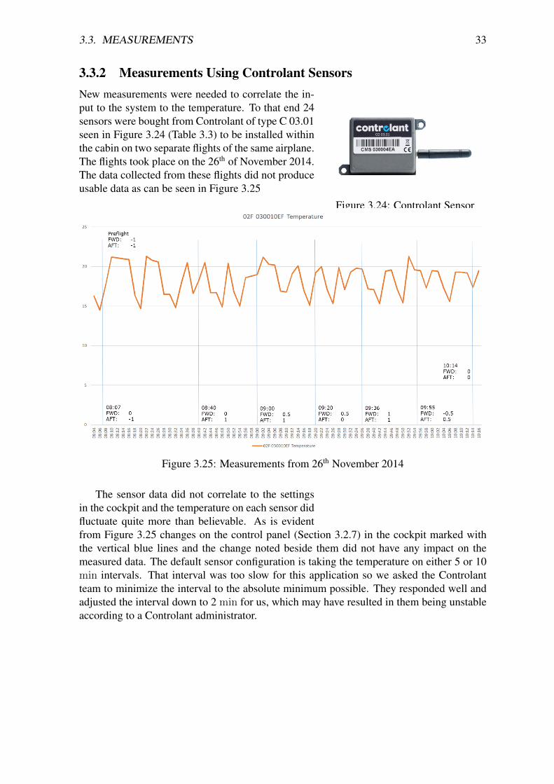
New measurements were needed to correlate the in-put to the system to the temperature. To that end 24sensors were bought from Controlant of type C 03.01seen in Figure 3.24 (Table 3.3) to be installed withinthe cabin on two separate flights of the same airplane.The flights took place on the 26th of November 2014.The data collected from these flights did not produceusable data as can be seen in Figure 3.25

Figure 3.25: Measurements from 26th November 2014

The sensor data did not correlate to the settingsin the cockpit and the temperature on each sensor didfluctuate quite more than believable. As is evidentfrom Figure 3.25 changes on the control panel (Section 3.2.7) in the cockpit marked withthe vertical blue lines and the change noted beside them did not have any impact on themeasured data. The default sensor configuration is taking the temperature on either 5 or 10min intervals. That interval was too slow for this application so we asked the Controlantteam to minimize the interval to the absolute minimum possible. They responded well andadjusted the interval down to 2 min for us, which may have resulted in them being unstableaccording to a Controlant administrator.


3.3.3 Measurements on Board an Empty Aircraft

Figure 3.26: EL-WIFI-TC & T-Probe

The last measurements to get the inputto the system correlated to the changesmade in the cockpit were undertaken on theground in an empty aircraft at Keflavik air-port on the 16th of April 2015. A new devicefrom Lascar electronics (Table 3.3) capableof logging at a 10 s interval was loaned tous from Samey ehf. The probe on that newdevice was a probe of PT-100 type which istoo slow for this application so a new T typeprobe was loaned to us from RJ Verkfræðin-gar. The sensor and the probe can be seen inFigure3.26. In this measurement session thechanges made in the cockpit on the controlpanel (Section 3.2.7) shows a response in the measured temperature. The placement insidethe cabin was at seat number 21D as shown in Figure 3.27. The temperature sensor itselfwas left hanging from the seat at approximately 20 cm from the floor. The measurementswere performed between 19:00 to 22:00 in the evening. The mean outside temperature overthe time it took to complete the measurements was 7C. The data collected from that sessionwas used as a starting point in the simulation.

Figure 3.27: Instrument placement in the cabin

Data collected that evening can be seen in Figure 3.28. The measurements were dividedinto seven time periods divided by the input to the system i.e. the control knob in the cockpit(see Section 3.2.7) which has settings from -3 (Cold) to +3 (Warm) where 0 (Auto) is in themiddle. Figure 3.28 Shows the measured data from the whole evening.


Figu

re3.

28:M

easu

red

data

37

Chapter 4

Results & Discussion

In the beginning a model was created of half of the whole aircraft, the slip/symmetry (subsec-tion 3.2.3.1) boundary condition is exactly suited for this to decrease the number of elementsneeded. It was simulated after extensive simplifications for that in the beginning it producedover 95 million elements when imported to ASCFD. Figure 4.1 shows the simulated airplanefull of passengers. This simulation produced just over 2 million elements when meshed andtherefore the solution time was quite long, measured in 3 days not hours. Even after all thesimplifications the element count was still too high for it to be reasonable to run simulationswith different settings for the duration of this project.

Figure 4.1: Half Plane, over 2 million elements

The simulation of the air flow through the half of the whole aircraft showed that therewere no dead spots or stagnant air pockets present in the plane. Figure 4.2 shows the com-puted air flow in the cabin, with all passengers present but hidden aside the ones showingof course for a better view of the flow itself. As Figure 4.2 demonstrates the airflow in thesimulation is well distributed over the whole of the cabin.

38 CHAPTER 4. RESULTS & DISCUSSION

Figure 4.2: Air Flow In The Cabin

The heat distribution throughout the cabin from measurements ITS carried out in severalflights showed that from front to back of the cabin the heat rises, the heat distribution fromthe simulation resembles that and can be read from Figure 4.3. From Figure 4.3 we seethat the passengers seated at the window row are generally 2 to 3 C colder than the onesseated at the isle which is exactly as it is in reality. It also shows how the temperature risesthroughout the cabin from front to back.

Figure 4.3: Passenger Comfort Temperature

39

Figure 4.4: PMV In Row 27

Figure 4.4 shows the PMV [12] (refer to 2.1.12) for passengers seated at row 27 in theaircraft. From the figure we can see that the passenger seated at the window is a bit colderthan the others which correlates exactly to the real world.


Figure 4.5: Simulated cabin

The time it took for the simulation to solve was aproblem because of the need to run many simulationswith different settings it would have taken monthsto complete. After some discussion it was decidedto make a new smaller surrogate for optimization ofthe cabin, which Figure 4.5 depicts. The smallermodel seen in Figure 4.5 had roughly 250.000 ele-ments which resulted in a much more reasonable so-lution time of about 3 - 4 hours per simulation run.This dramatic decrease in element count is largelybecause all circular and complex geometry was re-moved from the model in AIP. This process of sim-plifying when dealing with CFD problems is consid-ered to be the best practice[23] i.e. to take everythingthat doesn’t really matter to the simulation and delete it from the model. That does not affectthe air flow in this case because the air speed, where there are obstructions in the air flow,is always below 0.3m s−1 which does not influence the flow as it would at higher air speeds.This decrease in element count in ASCFD does not however influence the overall accuracyof neither the simulated air flow or the heat transfer computations of the model to a degreethat matters.

Before running the simulation the measured data seen in Figure 3.28 was divided intoseven time periods which all have a sample rate of 10s. Each time period started when thesystem was stable at the moment when the set point (input signal) was changed i.e. theheat setting in the cockpit. The simulation procedure for each measured time period wasperformed in the following way:

1. Starting temperature was set equal to the measured one

2. Initial inlet temperature (see subsection 3.2.3.2) was initially guessed

3. Time step size set to 1s

4. Number of time steps were set equal to the measured time period

5. Simulation was solved

6. Final simulated temperature compared to the measured final temperature → If sim-ulated final temperature was more than ±0.1C from the final measured temperatureinlet temperature was adjusted accordingly in the simulation

7. Iterate (run the simulation again from the beginning) until finishing temperature waswithin ±0.1C

To establish a baseline model from the simulations we needed to estimate the transferfunction (TF) from each time period. The TF provides a basis for determining importantsystem response characteristics without the need to solve the complete differential equationsfor a given system. A TF describes the ratio of the output of a system to the input of the samesystem. But we need to keep in mind that this is both an approximation and a linearizationof the “real” system. The Step Response (SR) is needed for the comparison of the measuredsystem to the simulated one. The SR of a system is the output of the system when a unit stepfunction is used as an input. That was chosen to be the best comparison method betweenthese two systems implemented by Matlab analysis.

41

When all simulated time periods were within set limits the data was exported from AS-CFD to a .cls file format. Excel was used to revert the .cls files to .xlsx files and then 10 fakepoints (zero padding) were added in front of all series due to a warning Matlab threw at thebeginning because the input signal started at 0 i.e. no time passed before the signal change.All the data was imported into Matlab using scripts (see Appendix C).

The time periods can be seen in Table 4.1. The simulations took from two to four runsto get all simulated temperature values within acceptable range of ±0, 1C. Table 4.1 showsthe time periods and the end result temperature from the simulations. As can be seen fromTable 4.1 the sample time is 10s. The last column (# 8) shows the end temperature of thesimulation which in all time periods is less than±0, 1C from the measured end temperaturein column 5.

Table 4.1: Simulation Tweaks

Periods Measured Values Simulation ValuesInlet Temp End Temp

Time Start End Start End# hh:mm:ss hh:mm:ss s C C C C

1 20:28:08 20:40:58 770 17.2 22.3 26.5 22.292 20:41:08 20:54:58 830 22.4 23.0 23.7 23.043 20:55:08 21:16:58 1310 23.0 24.2 25.2 24.154 21:17:08 21:29:58 770 24.1 26.7 29 26.705 21:30:08 21:41:28 680 26.6 29.3 31.8 29.336 21:41:38 21:46:58 320 29.4 30.0 30.9 30.047 21:47:08 22:03:38 990 30.4 24.0 19.3 23.97

Matlab has an inbuilt function which creates an identification object for the time-seriesdata:

data = iddata(y,u,Ts)

The “iddata” function creates a data object that contains a time-domain output signal “y”and input signal “u”, respectively. “Ts” specifies the sample time of the data which was setto being 10 s. The data objects created from the “iddata” function were then sent to anotherfunction which estimates a linear approximated continuous-time transfer function for theidentification object (“iddata”):

sys = tfest(data,np,nz)

The linear continuous-time transfer function, “sys”, is created using time- or frequencydomain data, number of poles (“np”), and number of zeros (“nz”), where the number ofzeros in the “sys” function is max(np − 1, 0). If the number of zeros (“nz”) to the functionisn’t set like in this case the zeroes are set to be one less than the poles which in this case isone. The number of poles from both the measured as well as the simulated data was set tobe two after trying out various of settings for the number of poles.

When the step response plots were diagnosed it became evident that the “tfest” func-tion resulted in unstable systems for some of the time periods. Because of these unstableproperties these time periods were excluded from the following sub chapters as they did not


produce any meaningful results. The results from the unstable time periods can be found inAppendix A. It is believed that this instability is because of a too short of a time period i.e.the systems were not stable enough coupled with a large overshoot in the measured temper-ature. For this reason measured time periods 3, 5, 6 and 7 were omitted from the results.Time period 5 was corrupted by the unexpected opening of the aircraft cabin shortly afterthe input signal was changed.

Table 4.2 shows the estimated data fit for the selected time periods both for the measured-and the simulated time periods. The fit value compute is the Normalized Root Mean SquareError (NRMSE) value, Final Prediction Error (FPE) and Mean Square Error (MSE).

Table 4.2: Fit Estimation data

NRMSE FPE MSE

Period # Meas Sim Meas Sim Meas Sim1 90,24% 93,67% 0,04558 0,01409 0,04011 0,0124002 75,51% 93,09% 0,02669 0,00026 0,02367 0,0002323 84,24% 93,85% 0,03366 0,0004812 0,03104 0,00044364 77,43% 93,53% 0,07845 0,00388 0,06903 0,0034185 83,31% 93,30% 0,06771 0,00491 0,05073 0,0042626 32,41% 90,92% 0,05203 0,0009013 0,04067 0,00070467 79,45% 93,11% 0,5854 0,02204 0,5088 0,01987

In the following subsections the results will be discussed for each individual usable timeperiod, refer to Appendix A for results from the time periods that were deemed unusable.

4.1. 1ST TIME PERIOD 20:28:08-20:40:58 43

4.1 1st Time Period 20:28:08-20:40:58

We start by looking at the time series from both the measured (from Figure 3.28) and thesimulated data plotted together in Figure 4.6.

Figure 4.6: Measured vs Simulated - Time Series - Time Period 1

In Figure 4.6 we see that the simulated time series follows the measured time seriesclosely from start to end. The measured time series are rather noisy which is believed tobe due to inaccuracies in the measurement device [22]. The delay of 100s in the beginningis because of the zero padding of 10 points. The temperature ends roughly the same asintended.

Next we take a look at Figure 4.7 where the step responses from the linearized modelsof those two systems are plotted together. The estimated linear transfer functions for boththe measured and the simulated data is given in Equation 4.1 and Equation 4.2 respectively.

H(s)Measured =0.01031s+ 0.000472

s2 + 0.01388s+ 0.0000911(4.1)

H(s)Simulated =0.05025s+ 0.0007823

s2 + 0.02932s+ 0.0001543(4.2)


Figure 4.7: Measured vs Simulated - Step Response - Time Period 1

From the graph in Figure 4.7 we see how well the measured system is simulated. But weneed to keep in mind that these are the approximated models, not the “true” systems. Thisis where it is most logical to make the comparison between these two systems. The aircraftsystem is a closed-loop system which results in the overshoot but the the simulated systemis an open-loop system which has no such capabilities. The only changeable variable in thesimulation is the inlet temperature (subsection 3.2.3.2).

Table 4.3 shows the comparison of key values from Matlab i.e. the rise time (10− 90%),settling time (2%), settling min, settling max and the overshoot.

Table 4.3: Stepinfo - Time Period 1

Name Measured Simulated

Rise Time 226.2 292.8Settling Time 595.3 537.5Settling Min 4.71 4.58Settling Max 5.37 5.06Overshoot 3.69 0

Table 4.3 and Figure 4.7 draws out the differences between these two systems where youhave a closed-loop controller in the aircraft vs the open-loop system for the simulation.

Figure 4.8 shows the step response and its corresponding time series plotted together.

4.1. 1ST TIME PERIOD 20:28:08-20:40:58 45

Figure 4.8: Measured Data - Time Series vs Step Response - Time Period 1

When the step response is plotted together with the time series for the measured data inFigure 4.8 we can see that it relates closely to the measured data. The noise in the measuredvalues is believed to be caused by inaccuracies in the measuring device. In Figure 4.9 Thesame plot is shown for the simulated data.

Figure 4.9: Simulated Data - Time Series vs Step Response - Time Period 1

Figure 4.9 shows well how very closely the linearized model relates to its time seriescounterpart.

From the graphs in Figure 4.8 and Figure 4.9 and from Figure 4.7 where the step re-sponses are plotted together from the two systems it is apparent that the simulated data


related very closely to the measured data. The question goes how good is the simulationcompared to the measured data? These two systems are fundamentally different as beforementioned i.e. the system on board the aircraft is probably at least a 2nd or a 3rd orderclosed-loop system with time delay whereas the simulated system is an open-loop system.Therefore it is logical to take a look at the steady state error which in this case is the finalvalue in the step response plots. The steady state error is calculated in Equation 4.3 from theconstant terms (zeroth-order terms) from Equation 4.1 and Equation 4.2:

A =0.05025s+0.0007823

s2 + 0.02932s+0.0001543= 5.07 B =

0.01031s+0.000472

s2 + 0.01388s+0.0000911= 5.18

Steady State Error = 1− A

B= 1− 5.07

5.18= 1− 0.97876 ≈ 2.1% (4.3)

This confirms that the simulation is well grounded to the measured data.

4.2 2nd Time Period 20:41:08-20:54:58We start as before by looking at the time series (Figure 3.28) from both the measured andthe simulated data plotted together in Figure 4.10.


In Figure 4.10 we see that the simulated time series have a large overshoot. The tem-perature does however end roughly the same for both as intended. It would be interestingto see if this behavior would repeat itself in another aircraft. The measurements do eventhough they are quite noisy show a large overshoot when the cockpit control knob for the airconditioning system is moved from -2 to -1. This could be intended but here the author ofthis thesis lacks the information needed to confirm that is indeed the case.

4.2. 2ND TIME PERIOD 20:41:08-20:54:58 47

Next we take a look at Figure 4.11 where the step responses from those two systems areplotted together. The estimated transfer functions for both the measured- and the simulateddata is given in Equation 4.4 and Euation 4.5 respectively.

H(s)Measured =0.01254s+ 0.00001764

s2 + 0.003895s+ 0.00002453(4.4)

H(s)Simulated =0.006027s+ 0.000008677

s2 + 0.01077s+ 0.00001386(4.5)


From the graph in Figure 4.11 we see the overshoot for the measured systems approx-imated step response. The time Matlab estimates for the system to become stable is morethan three times longer than the time series last. That suggests that more time would beneeded for the measured time series.




Rise Time 50.2 211.8Settling Time 2017 333.3Settling Min 0.39 0.56Settling Max 1.98 0.64Overshoot 174.8 0

Table 4.4 and Figure 4.11 confirm that either the measurement time was too short or thesystem is not functioning as intended at this setting.




When the step response is plotted together with the time series for the measured data inFigure 4.12 it becomes even more clear that the measurement time here is the likeliest culprit.But this result also demonstrates quite well how a baseline system could be used to identifyproblems in the air conditioning system given that the measurements were implemented ina standardized and correct way. In Figure 4.13 the step response for the simulated system isplotted with its corresponding time series. Even though the step response plot follows thesimulated time series very closely we see the similar behavior regarding the time estimatefor the system to get stable i.e. Matlab estimates that it would take more than twice as longthan time series actually are to get the system stable. From these result the author concludesthat the measurement time is too short.

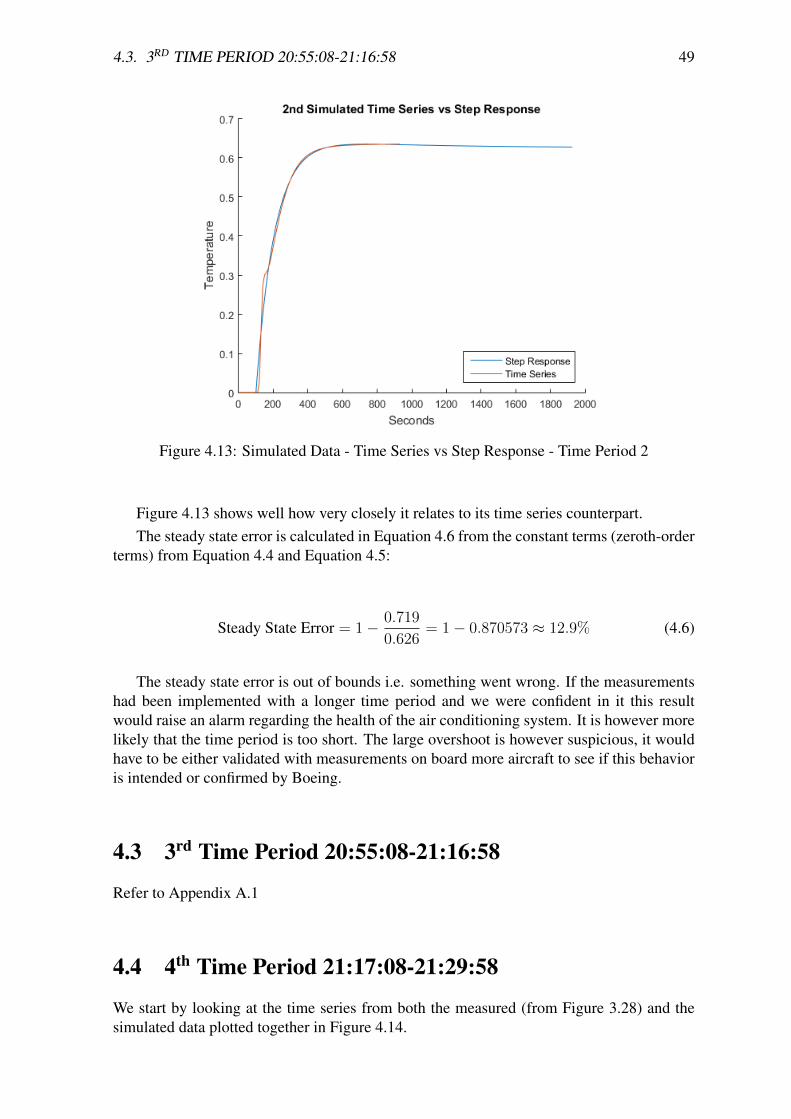
4.3. 3RD TIME PERIOD 20:55:08-21:16:58 49


Figure 4.13 shows well how very closely it relates to its time series counterpart.The steady state error is calculated in Equation 4.6 from the constant terms (zeroth-order

terms) from Equation 4.4 and Equation 4.5:

Steady State Error = 1− 0.719

0.626= 1− 0.870573 ≈ 12.9% (4.6)

The steady state error is out of bounds i.e. something went wrong. If the measurementshad been implemented with a longer time period and we were confident in it this resultwould raise an alarm regarding the health of the air conditioning system. It is however morelikely that the time period is too short. The large overshoot is however suspicious, it wouldhave to be either validated with measurements on board more aircraft to see if this behavioris intended or confirmed by Boeing.

4.3 3rd Time Period 20:55:08-21:16:58

Refer to Appendix A.1

4.4 4th Time Period 21:17:08-21:29:58

We start by looking at the time series from both the measured (from Figure 3.28) and thesimulated data plotted together in Figure 4.14.



In Figure 4.14 we see that apart from the overshoot in the measured data the simulateddata does correspond quite well to the time series. The temperature as before ends roughlythe same for both as intended.

Next we take a look at Figure 4.15 where the step responses from those two systemsare plotted together. To get the step responses we need the approximated TF. The estimatedtransfer functions for both the measured- and the simulated data is given in Equation 4.7 andEquation 4.8 respectively.

H(s)Measured =0.005919s+ 0.0004494

s2 + 0.008645s+ 0.0001692(4.7)

H(s)Simulated =0.02602s+ 0.0004911

s2 + 0.0328s+ 0.0001893(4.8)

4.4. 4TH TIME PERIOD 21:17:08-21:29:58 51


From the graph in Figure 4.15 we see how well the measured system is simulated apartfrom the overshoot they relate very closely together.




Rise Time 104.7 276.9Settling Time 841.2 503Settling Min 2.36 2.34Settling Max 3.55 2.59Overshoot 33.55 0

Table 4.5 illustrates how close the simulation is. The rise-, settling min- and the settlingmax times differ that much because of the overshoot.




The graph in Figure 4.16 shows that the estimated time for the system is like in timeperiod 2 extended before predicted stabilization is achieved but not as much this time. Thissuggests however again that this time period was too short too. In Figure 4.17 The same plotis shown for the simulated data.


The graph in Figure 4.17 shows that the time in the step response is extended far less thain time period 2 but extended anyway. That gives more confidence in drawing the conclusionthat the time periods in general need to be extended to be around at least 30min, but thatneeds to be tested for validation by measuring more aircraft.

4.5. 5TH TIME PERIOD 21:30:08-21:41:28 53

From the graphs in Figure 4.16 and Figure 4.17 and from Figure 4.15 where the stepresponses are plotted together from the two systems it is apparent that the simulated datarelated pretty closely to the measured data even though it seems that the time period wastoo short. The steady state error for this time period is calculated in Equation 4.9 from theconstant terms (zeroth-order terms) from Equation 4.7 and Equation 4.8:


2.59429= 1− 0.976757 ≈ 2.3% (4.9)

This confirms that the simulation is well grounded to the measured data despite themeasurement time being a little bit too short.

4.5 5th Time Period 21:30:08-21:41:28Refer to Appendix A.2



55

Chapter 5

Conclusions

5.1 SummaryAfter introducing Computational Fluid Dynamics (CFD), basic terminology and generalequations for fluid flow were explained. The general governing equations for CFD calcula-tions were presented and the three most popular discretization methods were introduced.

All geometry was modeled in Autodesk Inventor Professional (AIP). The 3D model fromAIP was then imported to Autodesk Simulation CFD (ASCFD) for the simulation. At thebeginning a half of all the aircraft was modeled and imported into ASCFD. No dead spotsor stagnant air pockets were present in the cabin as Figure 4.2 shows from the simulation ofthe whole cabin.

Figure 5.1: Halved Aircraft Model

Figure 5.2: The Slice

The time it took to run the simulation forthe whole aircraft was however measured in 3to 4 days not hours which would be acceptablein many cases but in this case where many set-tings and trial and error experiments were to takeplace it would take too long to solve each one. Inlight of this a smaller surrogate model for opti-mization was built and the model reduced downfrom the over 28m the cabin measures in realityto 3.2m with 3 seat rows from the mid section ofthe plane. Figure 5.1 shows the main dimensionsof the first model i.e. the half of the whole air-craft after extensive simplifications were madein order to reduce the element count to be ableto solve the model when imported to ASCFD.The cut down model referred to as “The Slice”as that is what it really is, a small portion of thecabin can be seen in Figure 5.2.

56 CHAPTER 5. CONCLUSIONS

Measurements were undertaken on board an empty aircraft at Keflavik airport on the16th of April 2015. The data from the empty aircraft contained seven time periods dividedby the input to the system i.e. the control knob in the cockpit which has settings from -3(Cold) to +3 (Warm) where 0 (Auto) is in the middle. All time periods were then simulatedusing “The Slice”. Upon diagnosing the data by using Matlab it became clear that a few ofthe time periods did not produce stable systems. The transfer function estimation process inMatlab predicted that the time to reach stability would be substantially longer. It is believedthat this behavior is due to the time periods being too short. For this reason time periods3, 5, 6 and 7 were excluded from the results chapter because these systems had not reachedequilibrium. The results from the excluded time periods can be seen in Appendix A. Thestarting temperature for each period was used in each corresponding simulation where theinlet temperature was tweaked until it gave the same end temperature as the measurements±0.1C. The results suggest that a standardized measurement procedure coupled with abaseline model would be a feasible choice to confirm whether an air conditioning system inan arbitrary aircraft of this type is functioning properly with respect to passenger comfort.

5.2 Final ThoughtsThe following main conclusions can be drawn from the project that has been carried out tobuild an analytical baseline model for the cabin environment of the Boeing 757-200 aircraft:

• A full fledged simulation of the entire cabin of the aircraft is a feasible albeit verydemanding in terms of computing performance for a standard workstation. Ideally itwould need to be solved using either a cloud service or a super computer. But thequestion remains whether that would be sensible or not.

• The simulation from the whole aircraft suggests that there are no dead spots or stag-nant air pockets present in the cabin. The heat distribution from the simulation isbelievable as it relates closely to actual temperature values from measurements Ice-landair Technical Services (ITS) carried out in several flights. Those measurementsshow that the heat rises from the front to the back of the aircraft to which the heatdistribution showed to be the same in both.

• The response from the cabin temperature to changes in the inlet temperature can beaccurately predicted by a simplified “slice” simulation model. This is a key to establisha baseline model for the cabin temperature and for assessing the performance of itscontrol system.

• The steady state error between the measured time periods and the simplified “slice”simulations was well within the acceptable range of 2.2%± 0.1% for the time periodscontaining plausible data.

• It is feasible to establish a baseline model to validate whether the control system onboard some chosen aircraft is functioning as intended. In order to verify and validatethis conclusion however, more measurements need to be taken from more than oneaircraft as is the case here, as it is not known whether this particular aircraft chosenfor the measurements is in fact exhibiting “normal” control system behavior.

5.3. FUTURE WORK 57

5.3 Future WorkTo establish a validated baseline model for comparison a number of tasks should be carriedout:

• The full model should be developed further with regards to simplifications e.g. inte-grate the hand luggage compartment to the shell as well as both the roof and the airinlet, seats do not need footing, etc.

• More measurements must be undertaken including more aircraft as that is necessaryto validate and establish how a “normal” control system behaves.

• The closed-loop control system should be modeled and included in the simulation.At this point limited information about the exact algorithm of the AC controller isavailable.

• A standardized measurement procedure preferably with fixed time periods should bedeveloped to determine the “health” of the cabin environmental system for the com-parison to the baseline model.

• Surveys should be integrated into the on board entertainment system. That could berewarded with early alarms should something go wrong in the air conditioning system.That would also emphasize that Icelandair “cares” for its passengers.

59

Acronyms

AIP Autodesk Inventor Professional. xii, xiii, 15, 40, 55

ASCFD Autodesk Simulation CFD. xii, xiii, 8, 9, 12, 13, 15, 19, 23, 24, 37, 40, 41, 55

BC Business Class. 18, 22

CAD Computer Aided Design. xii

CC Comfort Class. 18, 22

CFD Computational Fluid Dynamics. 1, 3, 4, 9, 11, 40, 55

EC Economy Class. 18, 22

FDM Finite Difference Method. 12

FEM Finite Element Method. 12, 13

FPE Final Prediction Error. 42

FVM Finite Volume Method. 13

ICBM Intercontinental Ballistic Missile. 3

ITS Icelandair Technical Services. xvii, 15, 31, 38, 56

MSE Mean Square Error. 42

NACA National Advisory Committee for Aeronautics. 3

NRMSE Normalized Root Mean Square Error. 42

PDES Partial Differential Equations. 12, 13

PMV Predicted Mean Vote. xxi, xxiii, 10, 39

PPD Predicted Percentage of Dissatisfied. 10

SR Step Response. 40

TF transfer function. 40, 51, Glossary: Transfer Function

61

Bibliography

[1] B. S. Massey, Mechanics of fluids, 8th ed. London ; New York: Taylor & Francis,2006, ISBN: 0415362067.

[2] J. Wendt, Computational Fluid Dynamics: An Introduction, en. Springer, Oct. 2008,ISBN: 9783540850564.

[3] H. Julian and A. J. Eggers, “A study of the motion and aerodynamic heating of bal-listic missiles entering the earth’s atmosphere at high supersonic speeds”, NationalAdvisory Committee for Aeronautics, Tech. Rep. 1381, 1958. [Online]. Available:http://digital.library.unt.edu/ark:/67531/metadc65613/m2/1/high_res_d/19930091020.pdf (visited on 04/25/2014).

[4] M. Abbett and G. Moretti, “A time-dependent computational method for blunt bodyflows.”, AIAA Journal, vol. 4, no. 12, pp. 2136–2141, 1966. [Online]. Available: http://arc.aiaa.org/doi/abs/10.2514/3.3867 (visited on 05/12/2014).

[5] Simulating swimwear for increased speed, Electronic. [Online]. Available: http://www.ansys.com/staticassets/ANSYS/staticassets/resourcelibrary/article/AA-V2-I2-Swimwear-for-Increased-Speed.pdf(visited on 03/14/2014).

[6] Autodesk help, Electronic. [Online]. Available: http://help.autodesk.com/view/SCDSE/2014/ENU/?guid=GUID-B737967D-DF1E-4A7E-AAED-CFD7FD41D0CD (visited on 04/18/2014).

[7] Mach number, Electronic. [Online]. Available: http://help.autodesk.com/view/SCDSE/2014/ENU/?guid=GUID-4DAF0D6D-F1F4-4E90-A9C8-5CACB85E79BE (visited on 04/18/2014).

[8] Density change as a function of the mach number, Electronic. [Online]. Available:http://www.aeromech.usyd.edu.au/aero/gasdyn/denvar1.gif(visited on 04/24/2014).

[9] N. Andersen and T. Rump, Varme ståbi, Danish. Kbh.: Nyt Teknisk Forlag, 2004,ISBN: 8757125465 9788757125467.

[10] F. P. Ole, Thermal comfort, 1970.

[11] F. Rohles and R. Nevins, “Nature of thermal comfort for sedentary man”, in ASHRAEJOURNAL, vol. 13, 1971, p. 58.

[12] A. Standard, “Standard 55-1992, thermal environmental conditions for human oc-cupancy, american society of heating, refrigerating and air conditioning engineers”,Refrigeration and Air-Conditioning Engineers, Inc., Atlanta, 1992.

http://digital.library.unt.edu/ark:/67531/metadc65613/m2/1/high_res_d/19930091020.pdf

http://digital.library.unt.edu/ark:/67531/metadc65613/m2/1/high_res_d/19930091020.pdf

http://arc.aiaa.org/doi/abs/10.2514/3.3867

http://arc.aiaa.org/doi/abs/10.2514/3.3867

http://www.ansys.com/staticassets/ANSYS/staticassets/resourcelibrary/article/AA-V2-I2-Swimwear-for-Increased-Speed.pdf



http://help.autodesk.com/view/SCDSE/2014/ENU/?guid=GUID-B737967D-DF1E-4A7E-AAED-CFD7FD41D0CD



http://help.autodesk.com/view/SCDSE/2014/ENU/?guid=GUID-4DAF0D6D-F1F4-4E90-A9C8-5CACB85E79BE



http://www.aeromech.usyd.edu.au/aero/gasdyn/denvar1.gif

62 BIBLIOGRAPHY

[13] N. Hashiguchi and Y. Tochihara, “Effects of low humidity and high air velocity in aheated room on physiological responses and thermal comfort after bathing: An exper-imental study”, International journal of nursing studies, vol. 46, no. 2, pp. 172–180,2009.

[14] Assessing thermal comfort results, Electronic. [Online]. Available: http://help.autodesk.com/view/SCDSE/2015/ENU/?guid=GUID-3283C0AF-B483-4897-970B-16A663ACF14E (visited on 05/28/2015).

[15] Galerkin’s method, Electronic. [Online]. Available: http://mathfaculty.fullerton.edu/mathews/n2003/GalerkinMod.html (visited on 04/25/2014).

[16] R. J. Schnipke, “A streamline upwind finite element method for laminar and turbulentflow”, Virginia Univ. Charlottsville, Tech. Rep., 1986. [Online]. Available: http://adsabs.harvard.edu/abs/1986PhDT........41S (visited on04/25/2014).

[17] Surface area of human skin, http://hypertextbook.com/facts/2001/IgorFridman.shtml.(visited on 04/27/2014).

[18] Persons and metabolic heat gain, Electronic. [Online]. Available: http://www.engineeringtoolbox.com/metabolic-heat-persons-d_706.html(visited on 04/14/2014).

[19] A. Standard, “Standard 161-2013, air quality within commercial aircraft, americansociety of heating, refrigerating and air conditioning engineers”, Refrigeration andAir-Conditioning Engineers, Inc., Atlanta, 2013.

[20] Slip/symmetry boundary condition, Electronic. [Online]. Available: http://help.autodesk.com/view/SCDSE/2015/ENU/?guid=GUID-9C1E28D5-B32E-4546-8620-7F428982184A (visited on 04/18/2014).

[21] How to choose an advection scheme in autodesk simulation cfd, Electonic. [Online].Available: http://help.autodesk.com/view/SCDSE/2014/ENU/?caas=caas/sfdcarticles/sfdcarticles/How-to-choose-an-advection-scheme-in-Autodesk-Simulation-CFD.html (visited on05/16/2014).

[22] Wifi thermocouple temperature data logging sensor, Electronic. [Online]. Available:https://www.dataloggerinc.com/datasheets/lascar/EL-WiFi-TC.pdf (visited on 04/14/2015).

[23] Geometry modeling techniques for aec applications, Electronic. [Online]. Available:http://help.autodesk.com/view/SCDSE/2015/ENU/?guid=GUID-9C1E28D5-B32E-4546-8620-7F428982184A (visited on 05/06/2015).

http://help.autodesk.com/view/SCDSE/2015/ENU/?guid=GUID-3283C0AF-B483-4897-970B-16A663ACF14E



http://mathfaculty.fullerton.edu/mathews/n2003/GalerkinMod.html

http://mathfaculty.fullerton.edu/mathews/n2003/GalerkinMod.html

http://adsabs.harvard.edu/abs/1986PhDT........41S

http://adsabs.harvard.edu/abs/1986PhDT........41S

http://www.engineeringtoolbox.com/metabolic-heat-persons-d_706.html

http://www.engineeringtoolbox.com/metabolic-heat-persons-d_706.html

http://help.autodesk.com/view/SCDSE/2015/ENU/?guid=GUID-9C1E28D5-B32E-4546-8620-7F428982184A



http://help.autodesk.com/view/SCDSE/2014/ENU/?caas=caas/sfdcarticles/sfdcarticles/How-to-choose-an-advection-scheme-in-Autodesk-Simulation-CFD.html



https://www.dataloggerinc.com/datasheets/lascar/EL-WiFi-TC.pdf

https://www.dataloggerinc.com/datasheets/lascar/EL-WiFi-TC.pdf



63

Appendix A

Unusable Data

A.1 3rd Time Period 20:55:08-21:16:58We start by looking at the time series from both the measured- and the simulated data plottedtogether in Figure A.1.

Figure A.1: Measured vs Simulated - Time Series - Time Period 3

In Figure A.1 we see that the simulated time series follows the measured time series justin the beginning, from there the measured temperature shows a massive overshoot. Thiswould need to be validated by measuring on board more aircraft to see if this behavior is theintended one. The temperature ends roughly the same for both as intended.

Next we take a look at the graph in Figure A.2 where the step responses from those twosystems are plotted together. The estimated transfer functions for both the measured- andthe simulated data is given in Equation A.1 and Equation A.2 respectively.

H(s) =0.009975s+ 0.00004902

s2 + 0.001872s+ 0.00002446(A.1)

64 APPENDIX A. UNUSABLE DATA

H(s) =0.01119s+ 0.000286

s2 + 0.03849s+ 0.0002547(A.2)

Figure A.2: Measured vs Simulated - Step Response - Time Period 3

The graph in Figure A.2 shows the resulting step responses. Because the measurementtime is to short the measured gain ends higher than it should because Matlab estimates theend result to be too high due to the time period being too short.

Table A.1 shows the comparison of key values from Matlab i.e. the rise time (10−90%),settling time (2%), settling min, settling max and the overshoot.

Table A.1: Stepinfo - Time Period 3


Variable Measured SimulatedRise Time 143.6 252.1Settling Time 4431 452.3Settling Min 1.10 1.01Settling Max 3.65 1.12Overshoot 82.2 0

Figure A.3 shows the measured step response and its corresponding time series plottedtogether.

A.1. 3RD TIME PERIOD 20:55:08-21:16:58 65

Figure A.3: Measured Data - Time Series vs Step Response - Time Period 3

When the step response is plotted together with the time series for the measured datain Figure A.3 we can see that it relates closely to the measured data but as is mentionedbefore the time period is too short so the estimation process in Matlab keeps on going. InFigure A.4 The same plot is shown for the simulated data.

Figure A.4: Simulated Data - Time Series vs Step Response - Time Period 3

The graph Figure A.4 confirms that the time period is too short and that neither systemis perceived being close to being stable.

From the graphs in Figure A.3 and Figure A.4 and from Figure A.2 where the step re-sponses are plotted together from the two systems it is apparent that the simulated data


related rather closely to the measured data apart from the large overshoot. The steady stateerror is calculated in Equation A.3 from the constant terms (zeroth-order terms) from Equa-tion A.1 and Equation A.2:


2.00409= 1− 0.560299 ≈ 44% (A.3)

The time period has to be prolonged.

A.2. 5TH TIME PERIOD 21:30:08-21:41:28 67

A.2 5th Time Period 21:30:08-21:41:28

We start by looking at the time series from both the measured- and the simulated data plottedtogether in Figure A.5.


In Figure A.5 the graph shows well how the time period got interrupted when the pas-senger cabin was opened unexpectedly shortly after the input signal was changed. Thistimeperiod is unusable for that sake.

H(s) =−0.003375s+ 0.00006247

s2 + 0.0000000000000004542s+ 0.00004485(A.4)

H(s) =0.02761s+ 0.0005448

s2 + 0.03369s+ 0.0001994(A.5)






Variable Measured SimulatedRise Time NaN 271.2Settling Time NaN 491.7Settling Min NaN 2.46Settling Max NaN 2.73Overshoot NaN 0


A.2. 5TH TIME PERIOD 21:30:08-21:41:28 69



The steady state error is calculated in Equation A.6 from the constant terms (zeroth-orderterms) from Equation A.4 and Equation A.5:


2.7322= 1− 0.509797 ≈ 49% (A.6)

The time period is unusable due to the opening of the passenger cabin.


A.3 6th Time Period 21:41:38-21:46:58



In Figure A.9 we can see that this time period is very short and therefore unusable.


H(s) =0.008661s− 0.00004658

s2 + 1.408 · 10−13s+ 0.0007605(A.7)

H(s) =0.008766s+ 0.00007454

s2 + 0.02249s+ 0.00008645(A.8)

A.3. 6TH TIME PERIOD 21:41:38-21:46:58 71





Variable Measured SimulatedRise Time NaN 349.9Settling Time NaN 686Settling Min NaN 0.78Settling Max NaN 0.86Overshoot NaN 0





The steady state error is calculated in Equation A.9 from the constant terms (zeroth-orderterms) from Equation A.7 and Equation A.8:


0.862233= 1− 0.071036 ≈ 93% (A.9)

The time period has to be prolonged to be able to read anything useful from the data.

A.4. 7TH TIME PERIOD 21:47:08-22:03:38 73

A.4 7th Time Period 21:47:08-22:03:38



From the graph in Figure A.13 the massive undershoot of the measured temperature. Thetime period is too short.


H(s) =0.007407s− 0.000004358

s2 + 4.613 · 10−8s+ 0.00000262(A.10)

H(s) =0.02305s+ 0.0001727

s2 + 0.02196s+ 0.00008101(A.11)



The graph in Figure A.14 shows the resulting step responses. Here it is evident that thesystem is regarded unstable at the end of the time period. Matlab estimates that the time itwould take to get the system stable very very long (2.5 · 108s). This result is a combinationof the too short of a time period and the massive undershoot. This measurement needs to berepeated on another aircraft to validate that this undershoot is the intended behavior.




Variable Measured SimulatedRise Time 2578 341.1Settling Time Nan 691.8Settling Min -6.49 1.92Settling Max 3.01 2.13Overshoot 290.1 0Undershoot 180.9 0


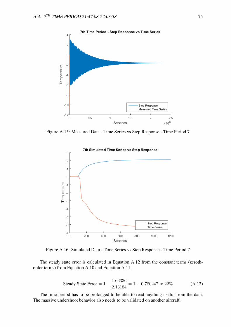
A.4. 7TH TIME PERIOD 21:47:08-22:03:38 75



The steady state error is calculated in Equation A.12 from the constant terms (zeroth-order terms) from Equation A.10 and Equation A.11:


2.13184= 1− 0.780247 ≈ 22% (A.12)

The time period has to be prolonged to be able to read anything useful from the data.The massive undershoot behavior also needs to be validated on another aircraft.

77

Appendix B

Air Speed To Cabin

79

Appendix C

Matlab

C.1 MData.m

1 %% Get measured data23 %% 1st Time Series 2028−20404 [~, ~, raw] = xlsread('D:\SVN_2015\project\cabin air quality\SIE\Inventor\

Icelandair_3D_Model_Slice\PV_2117_2129\Measured_data.xlsx','Sheet1','E2:E89');5 MT1 = reshape([raw:],size(raw));6 clearvars raw;7 [~, ~, raw] = xlsread('D:\SVN_2015\project\cabin air quality\SIE\Inventor\

Icelandair_3D_Model_Slice\PV_2117_2129\Measured_data.xlsx','Sheet1','F2:F89');8 MI1 = reshape([raw:],size(raw));9 clearvars raw;

1011 %% 2nd Time Series 2041−205412 [~, ~, raw] = xlsread('D:\SVN_2015\project\cabin air quality\SIE\Inventor\


Icelandair_3D_Model_Slice\PV_2117_2129\Measured_data.xlsx','Sheet1','F90:F183');16 MI2 = reshape([raw:],size(raw));17 clearvars raw;1819 %% 3rd Time Series 2055−211620 [~, ~, raw] = xlsread('D:\SVN_2015\project\cabin air quality\SIE\Inventor\


Icelandair_3D_Model_Slice\PV_2117_2129\Measured_data.xlsx','Sheet1','F184:F325');24 MI3 = reshape([raw:],size(raw));25 clearvars raw;2627 %% 4th Time Series 2117−212928 [~, ~, raw] = xlsread('D:\SVN_2015\project\cabin air quality\SIE\Inventor\



Icelandair_3D_Model_Slice\PV_2117_2129\Measured_data.xlsx','Sheet1','E414:E492');37 MT5 = reshape([raw:],size(raw));38 clearvars raw;

80 APPENDIX C. MATLAB

39 [~, ~, raw] = xlsread('D:\SVN_2015\project\cabin air quality\SIE\Inventor\Icelandair_3D_Model_Slice\PV_2117_2129\Measured_data.xlsx','Sheet1','F414:F492');

40 MI5 = reshape([raw:],size(raw));41 clearvars raw;4243 %% 6th Time Series 2141−214644 [~, ~, raw] = xlsread('D:\SVN_2015\project\cabin air quality\SIE\Inventor\




Icelandair_3D_Model_Slice\PV_2117_2129\Measured_data.xlsx','Sheet1','F536:F645');56 MI7 = reshape([raw:],size(raw));57 clearvars raw;

C.2 SData.m

1 %% Get simulation data23 %% 2028_20404 [~, ~, raw] = xlsread('D:\SVN_2015\project\cabin air quality\SIE\Inventor\

Icelandair_3D_Model_Slice\Simulation_AllPeriods\Sim_2028_2040_26dot5.xlsx','Sheet1','D2:D89');

5 ST1 = reshape([raw:],size(raw));6 clearvars raw;7 [~, ~, raw] = xlsread('D:\SVN_2015\project\cabin air quality\SIE\Inventor\

Icelandair_3D_Model_Slice\Simulation_AllPeriods\Sim_2028_2040_26dot5.xlsx','Sheet1','E2:E89');

8 SI1 = reshape([raw:],size(raw));9 clearvars raw;

10 %% 2041_205411 [~, ~, raw] = xlsread('D:\SVN_2015\project\cabin air quality\SIE\Inventor\




15 SI2 = reshape([raw:],size(raw));16 clearvars raw;17 %% 2055_211618 [~, ~, raw] = xlsread('D:\SVN_2015\project\cabin air quality\SIE\Inventor\





Icelandair_3D_Model_Slice\Simulation_AllPeriods\Sim_2117_2129_29.xlsx','Sheet1','D2:D89');26 ST4 = reshape([raw:],size(raw));27 clearvars raw;

C.3. SYSTEMANALYSIS.M 81

28 [~, ~, raw] = xlsread('D:\SVN_2015\project\cabin air quality\SIE\Inventor\Icelandair_3D_Model_Slice\Simulation_AllPeriods\Sim_2117_2129_29.xlsx','Sheet1','E2:E89');













50 SI7 = reshape([raw:],size(raw));51 clearvars raw;

C.3 SystemAnalysis.m

1 close all2 clear all3 clc45 %% Get data6 MData;7 SData;89 %% Create identification data objects

1011 MD1 = iddata(MT1,MI1,10);12 MD2 = iddata(MT2,MI2,10);13 MD3 = iddata(MT3,MI3,10);14 MD4 = iddata(MT4,MI4,10);15 MD5 = iddata(MT5,MI5,10);16 MD6 = iddata(MT6,MI6,10);17 MD7 = iddata(MT7,MI7,10);1819 SD1 = iddata(ST1,SI1,10);20 SD2 = iddata(ST2,SI2,10);21 SD3 = iddata(ST3,SI3,10);22 SD4 = iddata(ST4,SI4,10);23 SD5 = iddata(ST5,SI5,10);24 SD6 = iddata(ST6,SI6,10);25 SD7 = iddata(ST7,SI7,10);2627 %% Transfer function estimation


2829 MS1 = tfest(MD1,2);30 MS2 = tfest(MD2,2);31 MS3 = tfest(MD3,2);32 MS4 = tfest(MD4,2);33 MS5 = tfest(MD5,2);34 MS6 = tfest(MD6,2);35 MS7 = tfest(MD7,2);3637 SS1 = tfest(SD1,2);38 SS2 = tfest(SD2,2);39 SS3 = tfest(SD3,2);40 SS4 = tfest(SD4,2);41 SS5 = tfest(SD5,2);42 SS6 = tfest(SD6,2);43 SS7 = tfest(SD7,2);

C.4 CreatePlots.m

1 %% 1st Time Period − Meaured vs Simulated − 2028−20402 x1=0:10:870;3 figure('name','1st Time Period − Measured vs Simulated − 2028−2040')4 hold on5 plot(x1,MT1,x1,ST1);6 legend('Measured','Simulated','location','NorthEast')7 hold off8 title('1st Time Period − Time Series − Measured vs Simulated');9 xlabel('Seconds');

10 ylabel('Temperature');11 figure('name','1st Time Period − Step Response − Measured vs Simulated')12 hold on13 stepplot(MS1,SS1);14 legend('Measured','Simulated','location','SouthEast')15 hold off16 title('1st Time Period − Step Response − Measured vs Simulated');17 xlabel('Seconds');18 ylabel('Amplitude');1920 %% 2nd Time Period − Meaured vs Simulated − 2041−205421 x2=0:10:930;22 figure('name','2nd Time Period − Measured vs Simulated − 2041−2054')23 hold on24 plot(x2,MT2,x2,ST2);25 legend('Measured','Simulated','location','SouthEast')26 hold off27 title('2nd Time Period − Time Series − Measured vs Simulated');28 xlabel('Seconds');29 ylabel('Temperature');30 figure('name','2nd Time Period − Step Response − Measured vs Simulated')31 hold on32 stepplot(MS2,SS2);33 legend('Measured','Simulated','location','SouthEast')34 hold off35 title('2nd Time Period − Step Response − Measured vs Simulated');36 xlabel('Seconds');37 ylabel('Amplitude');3839 %% 3th Time Period 2055−211640 x3=0:10:1410;41 figure('name','3rd Time Period − Measured vs Simulated − 2055−2116')42 hold on43 plot(x3,MT3,x3,ST3);44 legend('Measured','Simulated','location','SouthEast')45 hold off46 title('3rd Time Period − Time Series − Measured vs Simulated');47 xlabel('Seconds');48 ylabel('Temperature');

C.4. CREATEPLOTS.M 83

49 figure('name','3rd Time Period − Step Respone − Measured vs Simulated')50 hold on51 stepplot(MS3,SS3);52 legend('Measured','Simulated','location','SouthEast')53 hold off54 title('3rd Time Period − Step Response − Measured vs Simulated');55 xlabel('Seconds');56 ylabel('Amplitude');5758 %% 4th Time Period 2117−212959 x4=0:10:870;60 figure('name','4th Time Period − Measured vs Simulated − 2117−2129')61 hold on62 plot(x4,MT4,x4,ST4);63 legend('Measured','Simulated','location','SouthEast')64 hold off65 title('4th Time Period − Time Series − Measured vs Simulated');66 xlabel('Seconds');67 ylabel('Temperature');68 figure('name','4th Time Period − Step Response − Measured vs Simulated')69 hold on70 stepplot(MS4,SS4);71 legend('Measured','Simulated','location','SouthEast')72 hold off73 title('4th Time Period − Step Response − Measured vs Simulated');74 xlabel('Seconds');75 ylabel('Amplitude');7677 %% 5th Time Period 2130−214178 x5=0:10:780;79 figure('name','5th Time Period − Measured vs Simulated − 2130−2141')80 hold on81 plot(x5,MT5,x5,ST5);82 legend('Measured','Simulated','location','SouthEast')83 hold off84 title('5th Time Period − Time Series − Measured vs Simulated');85 xlabel('Seconds');86 ylabel('Temperature');87 figure('name','5th Time Period − Step Response − Measured vs Simulated')88 hold on89 stepplot(MS5,SS5);90 legend('Measured','Simulated','location','SouthEast')91 hold off92 title('5th Time Period − Step Response − Measured vs Simulated');93 xlabel('Seconds');94 ylabel('Amplitude');9596 %% 6th Time Period 2141−214697 x6=0:10:420;98 figure('name','6th Time Period − Measured vs Simulated − 2141−2146')99 hold on

100 plot(x6,MT6,x6,ST6);101 legend('Measured','Simulated','location','SouthEast')102 hold off103 title('6th Time Period − Time Series − Measured vs Simulated');104 xlabel('Seconds');105 ylabel('Temperature');106 figure('name','6th Time Period − Step Response − Measured vs Simulated')107 hold on108 stepplot(MS6,SS6);109 legend('Measured','Simulated','location','SouthEast')110 hold off111 title('6th Time Period − Step Response − Measured vs Simulated');112 xlabel('Seconds');113 ylabel('Amplitude');114115 %% 7th Time Period 2147−2203116 x7=0:10:1090;117 figure('name','7th Time Period − Measured vs Simulated − 2147−2203')118 hold on


119 plot(x7,MT7,x7,ST7);120 legend('Measured','Simulated','location','SouthEast')121 hold off122 title('7th Time Period − Time Series − Measured vs Simulated');123 xlabel('Seconds');124 ylabel('Temperature');125 figure('name','7th Time Period − Step Response − Measured vs Simulated')126 hold on127 stepplot(MS7,SS7);128 legend('Measured','Simulated','location','SouthEast')129 hold off130 title('7th Time Period − Step Response − Measured vs Simulated');131 xlabel('Seconds');132 ylabel('Amplitude');133134 %% Time Periods vs Step Response for measured values135 % Zero padding136 add = zeros(10,1);137138 %% 1st Time Period − Step Response vs Time Series139 [mtemp1,mtime1] = step(MS1);140141 mtime1 = mtime1+100;142 mtime1 = vertcat(add,mtime1);143 mtemp1 = vertcat(add,mtemp1);144145 figure('name','1st Time Period − Step Response vs Time Series')146 hold on147 plot(mtime1,mtemp1);148 plot(x1,MT1);149 legend('Step Response','Measured Time Series','location','SouthEast')150 hold off151 title('1st Time Period − Step Response vs Measured Time Series');152 xlabel('Seconds');153 ylabel('Temperature');154155 %% 2nd Time Period − Step Response vs Time Series156 [mtemp2,mtime2] = step(MS2);157158 mtime2 = mtime2+100;159 mtime2 = vertcat(add,mtime2);160 mtemp2 = vertcat(add,mtemp2);161162 figure('name','2nd Time Period − Step Response vs Time Series')163 hold on164 plot(mtime2,mtemp2);165 plot(x2,MT2);166 legend('Step Response','Measured Time Series','location','SouthEast')167 hold off168 title('2nd Time Period − Step Response vs Measured Time Series');169 xlabel('Seconds');170 ylabel('Temperature');171172 %% 3rd Time Period − Step Response vs Time Series173 [mtemp3,mtime3] = step(MS3);174175 mtime3 = mtime3+100;176 mtime3 = vertcat(add,mtime3);177 mtemp3 = vertcat(add,mtemp3);178179 figure('name','3rd Time Period − Step Response vs Time Series')180 hold on181 plot(mtime3,mtemp3);182 plot(x3,MT3);183 legend('Step Response','Measured Time Series','location','SouthEast')184 hold off185 title('3rd Time Period − Step Response vs Measured Time Series');186 xlabel('Seconds');187 ylabel('Temperature');188


189 %% 4th Time Period − Step Response vs Time Series190 [mtemp4,mtime4] = step(MS4);191192 mtime4 = mtime4+100;193 mtime4 = vertcat(add,mtime4);194 mtemp4 = vertcat(add,mtemp4);195196 figure('name','4th Time Period − Step Response vs Time Series')197 hold on198 plot(mtime4,mtemp4);199 plot(x4,MT4);200 legend('Step Response','Measured Time Series','location','SouthEast')201 hold off202 title('4th Time Period − Step Response vs Measured Time Series');203 xlabel('Seconds');204 ylabel('Temperature');205206 %% 5th Time Period − Step Response vs Time Series207 [mtemp5,mtime5] = step(MS5);208209 mtime5 = mtime5+100;210 mtime5 = vertcat(add,mtime5);211 mtemp5 = vertcat(add,mtemp5);212213 figure('name','5th Time Period − Step Response vs Time Series')214 hold on215 plot(mtime5,mtemp5);216 plot(x5,MT5);217 legend('Step Response','Measured Time Series','location','SouthEast')218 hold off219 title('5th Time Period − Step Response vs Measured Time Series');220 xlabel('Seconds');221 ylabel('Temperature');222223 %% 6th Time Period − Step Response vs Time Series224 [mtemp6,mtime6] = step(MS6);225226 mtime6 = mtime6+100;227 mtime6 = vertcat(add,mtime6);228 mtemp6 = vertcat(add,mtemp6);229230 figure('name','6th Time Period − Step Response vs Time Series')231 hold on232 plot(mtime6,mtemp6);233 plot(x6,MT6);234 legend('Step Response','Measured Time Series','location','SouthEast')235 hold off236 title('6th Time Period − Step Response vs Measured Time Series');237 xlabel('Seconds');238 ylabel('Temperature');239240 %% 7th Time Period − Step Response vs Time Series241 [mtemp7,mtime7] = step(MS7);242243 mtime7 = mtime7+100;244 mtime7 = vertcat(add,mtime7);245 mtemp7 = vertcat(add,mtemp7);246247 figure('name','7th Time Period − Step Response vs Measured Time Series')248 hold on249 plot(mtime7,mtemp7);250 plot(x7,MT7);251 legend('Step Response','Measured Time Series','location','SouthEast')252 hold off253 title('7th Time Period − Step Response vs Time Series');254 xlabel('Seconds');255 ylabel('Temperature');256257 %% Time Periods vs Step Response for simulated values258


259 %% 1st Time Period − Step Response vs Time Series260 [stemp1,stime1] = step(SS1);261262 stime1 = stime1+100;263 stime1 = vertcat(add,stime1);264 stemp1 = vertcat(add,stemp1);265266 figure('name','1st Time Period − Step Response vs Simulated Time Series')267 hold on268 plot(stime1,stemp1);269 plot(x1,ST1);270 legend('Step Response','Time Series','location','SouthEast')271 hold off272 title('1st Simulated Time Series vs Step Response');273 xlabel('Seconds');274 ylabel('Temperature');275276 %% 2nd Time Period − Step Response vs Time Series277 [stemp2,stime2] = step(SS2);278279 stime2 = stime2+100;280 stime2 = vertcat(add,stime2);281 stemp2 = vertcat(add,stemp2);282283 figure('name','2nd Time Period − Step Response vs Simulated Time Series')284 hold on285 plot(stime2,stemp2);286 plot(x2,ST2);287 legend('Step Response','Time Series','location','SouthEast')288 hold off289 title('2nd Simulated Time Series vs Step Response');290 xlabel('Seconds');291 ylabel('Temperature');292293 %% 3rd Time Period − Step Response vs Time Series294 [stemp3,stime3] = step(SS3);295296 stime3 = stime3+100;297 stime3 = vertcat(add,stime3);298 stemp3 = vertcat(add,stemp3);299300 figure('name','3rd Time Period − Step Response vs Simulated Time Series')301 hold on302 plot(stime3,stemp3);303 plot(x3,ST3);304 legend('Step Response','Time Series','location','SouthEast')305 hold off306 title('3rd Simulated Time Series vs Step Response');307 xlabel('Seconds');308 ylabel('Temperature');309310 %% 4th Time Period − Step Response vs Time Series311 [stemp4,stime4] = step(SS4);312313 stime4 = stime4+100;314 stime4 = vertcat(add,stime4);315 stemp4 = vertcat(add,stemp4);316317 figure('name','4th Time Period − Step Response vs Simulated Time Series')318 hold on319 plot(stime4,stemp4);320 plot(x4,ST4);321 legend('Step Response','Time Series','location','SouthEast')322 hold off323 title('4th Simulated Time Series vs Step Response');324 xlabel('Seconds');325 ylabel('Temperature');326327 %% 5th Time Period − Step Response vs Time Series328 [stemp5,stime5] = step(SS5);


329330 stime5 = stime5+100;331 stime5 = vertcat(add,stime5);332 stemp5 = vertcat(add,stemp5);333334 figure('name','5th Time Period − Step Response vs Simulated Time Series')335 hold on336 plot(stime5,stemp5);337 plot(x5,ST5);338 legend('Step Response','Time Series','location','SouthEast')339 hold off340 title('5th Simulated Time Series vs Step Response');341 xlabel('Seconds');342 ylabel('Temperature');343344 %% 6th Time Period − Step Response vs Time Series345 [stemp6,stime6] = step(SS6);346347 stime6 = stime6+100;348 stime6 = vertcat(add,stime6);349 stemp6 = vertcat(add,stemp6);350351 figure('name','6th Time Period − Step Response vs Simulated Time Series')352 hold on353 plot(stime6,stemp6);354 plot(x6,ST6);355 legend('Step Response','Time Series','location','SouthEast')356 hold off357 title('6th Simulated Time Series vs Step Response');358 xlabel('Seconds');359 ylabel('Temperature');360361 %% 7th Time Period − Step Response vs Time Series362 [stemp7,stime7] = step(SS7);363364 stime7 = stime7+100;365 stime7 = vertcat(add,stime7);366 stemp7 = vertcat(add,stemp7);367368 figure('name','7th Time Period − Step Response vs Simulated Time Series')369 hold on370 plot(stime7,stemp7);371 plot(x7,ST7);372 legend('Step Response','Time Series','location','SouthEast')373 hold off374 title('7th Simulated Time Series vs Step Response');375 xlabel('Seconds');376 ylabel('Temperature');

School of Science and EngineeringReykjavík UniversityMenntavegur 1101 Reykjavík, IcelandTel. +354 599 6200Fax +354 599 6201www.ru.is

www.ru.is

boeing 757-200 interior simulation for cabin air quality ... · boeing 757-200 interior simulation...

Documents