black’s leverage eﬀect is not due to...

Electronic copy available at: http://ssrn.com/abstract=1762363

Black’s Leverage Effect

Is Not Due To Leverage∗

Jasmina Hasanhodzic† and Andrew W. Lo‡

This Draft: February 15, 2011

Abstract

One of the most enduring empirical regularities in equity markets is the inverse relationshipbetween stock prices and volatility, first documented by Black (1976) who attributed it tothe effects of financial leverage. As a company’s stock price declines, it becomes more highlyleveraged given a fixed level of debt outstanding, and this increase in leverage induces ahigher equity-return volatility. In a sample of all-equity-financed companies from January1972 to December 2008, we find that the leverage effect is just as strong if not stronger,implying that the inverse relationship between price and volatility is not driven by financialleverage.

Keywords: Volatility; Leverage Effect; Return/Volatility Relationship; Time-Varying Ex-pected Return; Behavioral Finance.

JEL Classification: G12

∗The views and opinions expressed in this article are those of the authors only, and do not necessarilyrepresent the views and opinions of AlphaSimplex Group, MIT, or any of their affiliates and employees. Theauthors make no representations or warranty, either expressed or implied, as to the accuracy or completenessof the information contained in this article, nor are they recommending that this article serve as the basis forany investment decision—this article is for information purposes only. Research support from AlphaSimplexGroup and the MIT Laboratory for Financial Engineering is gratefully acknowledged.

†Boston University and AlphaSimplex Group, Boston, MA, (646) 338–1971 (voice), [email protected] (email).‡Harris & Harris Group Professor, MIT Sloan School of Management, and Chief Investment Strategist,

AlphaSimplex Group, LLC. Corresponding author: Andrew W. Lo, MIT Sloan School of Management,E52–454, 50 Memorial Drive, Cambridge, MA 02142, (617) 253–0920 (voice), [email protected] (email).

Electronic copy available at: http://ssrn.com/abstract=1762363

Contents

1 Introduction 1

2 Literature Review 2

3 Data 7

4 Empirical Evidence 8

5 Conclusion 14

A Appendix 19

1 Introduction

One of the most enduring empirical regularities of equity markets is the fact that stock-return

volatility rises after price declines, with larger declines inducing greater volatility spikes. In

a seminal paper, Black (1976) provides a compelling explanation for this phenomenon in

terms of the firm’s financial leverage: a negative return implies a drop in the value of the

firm’s equity, increasing its leverage which, in turn, leads to higher equity-return volatility.

This explanation has been so tightly coupled with the empirical phenomenon that the inverse

relation between stock returns and volatility is now commonly known as the “leverage effect”.

This effect, and the leverage-based explanation, have been empirically confirmed by a number

of studies since Black (1976), e.g., Christie (1982), Cheung and Ng (1992), and Duffee (1995),

using linear regressions of returns on subsequent changes in volatility for individual stocks

and stock portfolios, and arguing that these relationships become stronger as the firms’ debt-

to-equity ratios increase. However, the validity of the leverage explanation has been called

into question more recently by Figlewski and Wang (2000), who document several empirical

anomalies associated with it.

In this paper we provide clear evidence that the leverage effect is not due to financial

leverage. Using the returns of all-equity-financed companies from January 1972 to December

2008, and the specifications of Black (1976), Christie (1982), and Duffee (1995), we find just

as strong an inverse relationship between returns and the subsequent volatility changes as

for their debt-financed counterparts. This finding suggests that we must look elsewhere for

an explanation of this empirical regularity, e.g., time-varying expected returns, endogenous

volatility, or path-dependent cognitive risk perceptions.

In Section 2 we provide a review of the literature in which the stock-return/volatility

relationship is documented, focusing on a few key regression-based studies that we replicate

using the sample of all-equity-financed companies described in Section 3. In Section 4 we

present our empirical results, and we conclude in Section 5 with a discussion of some possible

interpretations.

1

2 Literature Review

Black (1976) is widely credited as the originator of the leverage-effect literature. In his

pioneering paper, Black uses daily data from 1964 to 1975 of a sample of 30 stocks (mostly

Dow Jones Industrials) to study the relationship between volatility changes and returns in

individual stocks and the portfolio of those stocks. For each stock, Black constructs 21-day

summed returns, and estimates volatility over these intervals with the square root of the

sum of squared returns. The portfolio-level equivalents of these estimates, which he calls the

“summed market return” and the “market volatility estimate”, are obtained by averaging

the summed returns and the volatility estimates, respectively, across the sample of stocks.

He then defines the “volatility change” as the difference between the volatility estimate of

the current and the previous period, divided by the volatility estimate of the previous period,

and regresses the volatility change at time t+1 on the summed return at time t. His results

suggest a strong inverse relationship between the two: a 1% summed-return decline implies

a more than 1% volatility increase.

Black (1976) proposes two possible explanations for this relationship. The first explana-

tion, which he terms the “direct causation” effect, refers to the causal relation from stock

returns to volatility changes. A drop in the value of the firm’s equity will cause a negative

return on its stock and will increase the leverage of the stock (i.e., its debt/equity ratio),

and this rise in the debt/equity ratio will lead to a rise in the volatility of the stock. A

similar effect may arise even if the firm has almost no debt because of the presence of so-

called “operating leverage” (fixed costs that cannot be eliminated, at least in the short run,

hence when expected revenues fall, profit margins decline as well). The second explanation,

which Black (1976) calls the “reverse causation” effect, refers to the causal relationship from

volatility changes to stock returns. Changes in tastes and technology lead to an increase

in the uncertainty about the payoffs from investments. Because of the increase in expected

future volatility, stock prices must fall, so that the expected return from the stock rises to

induce investors to continue to hold the stock.

Using a sample of 379 stocks from 1962 to 1978, Christie (1982) estimates the following

linear relationship between changes in volatility from one quarter to the next and the return

2

over the first quarter for each stock:

ln(σt

σt−1

) = β0 + θSrt−1 + ut (1)

where σt−1 and rt−1 are the volatility estimate and return of the stock over quarter t−1.

He finds the cross-sectional mean elasticity to be −0.23, consistent with the leverage effect,

and then derives testable implications of various volatility models and efficient estimation

procedures to investigate the implications of risky debt and interest-rate changes on this

relationship. He finds significant positive association between equity volatility and financial

leverage, but the strength of this association declines with increasing leverage. Christie

finds that, contrary to the predictions stemming from the contingent claims literature, the

riskless interest rate and financial leverage jointly have a substantial positive impact on the

volatility of equity. Finally, he tests the elasticity hypothesis, which says that the observed

negative elasticity of equity volatility with respect to the value of equity is, in large measure,

attributable to financial leverage. For this purpose he uses the constant elasticity of variance

(CEV) model for equity prices, according to which σS = λSθ, and estimates the linear

regression:

ln(σS,t) = ln(λ) + θ ln(St) + ut (2)

where σS,t is the volatility estimated over quarter t, and St is the stock price at the beginning

of that quarter. He performs two separate tests of the hypothesis that θS is a function of

financial leverage—one based on leverage quartiles and the other on sub-periods—and finds

evidence in support of this hypothesis from both.

Cheung and Ng (1992) examine the inverse relation between future stock volatility and

current stock prices using daily returns of 252 NYSE-AMEX stocks with no missing returns

from 1962 to 1989, under the assumption of an exponential GARCH model for stock prices

(to control for heteroskedasticity and possible serial correlation in their returns). In this

model, the conditional variance equation has the logarithm of the lagged stock price on the

right-hand side, hence the corresponding coefficient θ is a measure of the leverage effect.

Applying the Spearman rank correlation test, the authors find a strong positive correlation

3

between θ and firm size, and explain this pattern by arguing that the smaller the firm,

the higher the debt/equity ratio. Their sub-sample analysis shows that the strength of

this relationship changes over time. In particular, conditional variances of stock returns on

average have become less sensitive to changes in stock prices over time, which, the authors

suggest, may be due to an increase in the firms’ liquidity over the sample period.

Duffee (1995) provides a new interpretation for the negative relationship between current

stock returns and changes in future stock return volatility at the firm level by arguing that

it is mainly due to a positive contemporaneous relationship between returns and volatility.

In addition to the usual test of leverage effect based on lagged returns, Duffee estimates the

following two contemporaneous regressions:

ln(σt) = α1 + λ1rt + εt,1 (3)

ln(σt+1) = α2 + λ2rt + εt+1,2 (4)

and observes that the usual lagged stock-return coefficient is simply the difference λ0 ≡

λ2− λ1. Using data for 2,500 firms traded on the AMEX or NYSE from 1977 to 1991 (not

necessarily continuously for the entire sample),1 Duffee finds that for a typical firm, λ1 is

strongly positive, λ2 is positive at the daily frequency and negative at the monthly frequency,

and that regardless of the sign of λ2, it is the case that λ1>λ2, implying that λ0<0. Duffee

then tests the theory behind the leverage effect, according to which highly leveraged firms

should have a stronger negative relation between stock returns and volatility than less highly

leveraged firms. Prior to his study, researchers have documented that the inverse relation

between period t stock returns and changes in the stock return volatility from period t to

period t+1 is stronger for firms with larger debt/equity ratios (e.g., Christie, 1982 and Cheung

and Ng, 1992), and that this relation is stronger for smaller firms (Cheung and Ng, 1992).

Using the Spearman rank correlations between the individual-firm regression coefficients (λ0,

λ1, and λ2) and debt/equity ratios and market capitalizations, Duffee obtains the following

1It is worth noting that, unlike Black (1976), Christie (1982), and Cheung and Ng (1992) who includeonly companies that were continuously traded throughout their sample periods, Duffee’s (1995) sample isbroader, including both continuously traded firms and those that exit the sample, which greatly reducessurvivorship bias. He finds that continuously traded firms are, on average, much larger and have lowerdebt/equity ratios than the typical firm.

4

three findings: First, the negative relation between λ0 and the debt/equity ratio found by

Christie (1982) and Cheung and Ng (1992) is confirmed only with monthly data for the

subset of continuously traded firms. When a larger sample of firms without survivorship

bias is used, the correlation between λ0 and the debt/equity ratio turns positive. Second,

highly leveraged firms exhibit stronger negative relations between stock returns and volatility

than less highly leveraged firms (the rank correlations between λ1 and the debt/equity ratio,

and λ2 and the debt/equity ratio, are both negative). And third, because the leverage

effect theory has no implications for the strength of the contemporaneous relation between

stock returns and volatility, Duffee argues that there is some reason other than the leverage

effect that is causing at least part of the correlation between firm debt/equity ratios and the

regression coefficients, and determining the negative correlation between the firm debt/equity

ratio and λ1. Furthermore, in accordance with Cheung and Ng (1992), he finds that λ0 is

positively correlated with size, at both monthly and daily frequencies, for all firms as well

as the sub-sample of continuously traded firms.

Our results differ from Duffie’s in a few important ways. First, Duffee’s conclusions apply

to the typical firm, whereas ours involve the extreme case of all-equity-financed companies.

Second, Duffee’s findings are mixed—as discussed above, he finds that the relationship be-

tween stock returns and volatility changes is negative for continuously traded firms, but

positive for the entire sample of firms—but we find a negative relationship in both contin-

uously traded and all firms in our sample of all-equity financed companies. Moreover, we

compare the relationship between stock returns and volatility changes of all-equity-financed

companies to that of their debt-financed counterparts, and find that the former is at least

as negative as the latter. These results lead us to conclude that rather than being the result

of leverage, the inverse relationship between average return and volatility is due to human

cognitive perceptions of risk (see Section 5). Although Duffee also suggests that something

other than leverage must be causing the correlation between firm debt/equity ratios and the

regression coefficients, he is motivated by his consideration of the contemporaneous relation

between returns and volatility changes for a typical firm, rather than by the lagged relation

between returns and volatility changes (the traditional “leverage effect” relationship) for

all-equity-financed firms and debt-financed firms separately.

Other explanations for the inverse relation between stock volatility and lagged returns

5

have been proposed, each developing into its own strand of literature. The most prominent

of these strands is the time-varying risk premia literature, according to which an increase in

return volatility implies an increase in the future required expected return of the stock, hence

a decline in the current stock price. In addition, due to the persistent nature of volatility

(large realizations of either good or bad news increase both current and future volatility),

a feedback loop is created: the increased current volatility raises expected future volatility

and, therefore, expected future returns, causing stock prices to fall now. The time-varying

risk premia explanation, also known as the volatility feedback effect, has been considered

by Pindyck (1984), French, Schwert, and Stambaugh (1987), and Campbell and Hentschel

(1992), typically using aggregate market returns within a GARCH framework.

Yet another explanation for the inverse relation between volatility and lagged returns,

first proposed by Schwert (1989) involves the apparent asymmetry in the volatility of the

macroeconomic variables. Empirical evidence suggests that real variables are more volatile

in recessions than expansions, hence, if a recession is expected but not yet realized, i.e., GDP

growth is forecasted to be lower in the future, stock prices will fall immediately, followed by

higher stock-return volatility when the recession is realized.

Disentangling these effects has proved to be a challenging task. For example, using

the data for the portfolios of Nikkei 225 stocks and a conditional CAPM model with a

GARCH-in-mean parametrization, Bekaert and Wu (2000) reject the leverage model and

find support for the volatility feedback explanation. In contrast, examining the relationship

between volatility and past and future returns using the S&P 500 futures high-frequency

data, Bollerslev, Litvinova, and Tauchen (2006) find that the correlations between absolute

high-frequency returns and current and past high-frequency returns are significantly negative

for several days, lending support to the leverage explanation, whereas the reverse cross-

correlations are negligible, which is inconsistent with the volatility feedback story.

Using the data for the individual stocks in the S&P 100 index, as well the aggregate index

data itself, Figlewski and Wang (2000) document a strong inverse volatility/lagged-return

relation associated with negative returns, but also a number of anomalies that cast some

doubt on the leverage-based explanation. Specifically, the inverse relation becomes much

weaker when positive returns reduce leverage, it is too small with measured leverage for

individual firms and too large when implied volatilities are used, and the volatility change

6

associated with a given change in leverage seems to decay over several months. Most impor-

tantly, there is no change in volatility when leverage changes due to a change in outstanding

debt or shares, but is observed only with stock-price changes, leading Figlewski and Wang

(2000) to propose a new label for the observed inverse volatility/lagged-return relation: the

“down-market effect”.

3 Data

Our sample consists of daily stock returns from the University of Chicago’s Center for

Research in Security Prices, and quarterly fundamental data from the CRSP/Compustat

Merged Database (Fundamentals Quarterly). We select only those stocks with zero total

debt for all quarters from January 1961 to December 2008, where total debt is defined as the

sum of total long-term debt, debt in current liabilities (short-term debt), and total preferred

stock.2 This filter yields 667 companies, which is our sample of all-equity financed (AE)

companies.

We also construct a complementary sample of companies with positive levels of total debt

in their capital structure in every quarter from January 1961 to December 2008, which yields

a considerably larger sample of 11,504 debt-financed companies. From this universe of debt-

financed (DF) companies, we select a smaller subset of 667 companies to match the number

of companies in our AE subset. This subset is selected by first sorting the AE companies

into size quintiles based on their median market capitalizations during the entire sample

period (where quintile breakpoints are computed from the entire CRSP Monthly Master

file), and then randomly selecting the same number of DF companies from each size quintile.

This procedure yields a matching sample of DF companies with approximately the same size

distribution as the AE sample.3 We then construct the subsets of the AE and DF monthly

datasets consisting of continuously traded firms for the 15-year period from January 3, 1994

2We first eliminate observations for which any of the long-term debt, current liabilities, or preferred stockis missing. Note that our definition of total debt differs slightly from Christie’s (1982), in which short-termdebt is measured by the accounting variable “current liabilities” (Compustat mnemonic LCT). This variableis comprised of four components: accounts payable (AP), current liabilities – other – total (LCO), debt incurrent liabilities (DLC), and income taxes payable (TXP). Since our filter is intended to separate companieswith and without debt in their capital structures, we use DLC as our measure of short-term debt.

3In particular, our AE sample contains 123, 109, 154, 188, and 93 companies in size quintiles 1 to 5,respectively.

7

to December 31, 2008. This time span was chosen as the best compromise to maximize the

number of time-series observations (15 years of daily returns) while maintaining a sufficiently

representative sample size of companies in the AE and DF sub-samples (23 continuously

listed AE firms and 41 continuously listed DF firms).

Finally, for each of the four samples (AE, DF, and their continuously listed sub-samples),

we obtain daily returns from the CRSP Daily Database, and to maintain the same start date

for the AE and DF companies, we use the later start date of December 18, 1972.

4 Empirical Evidence

We test the leverage effect using linear regression models where the dependent and inde-

pendent variables of the regression are those proposed by Black (1976), Christie (1982), and

Duffee (1995); using all three specifications serves as a robustness check on our results. To ob-

tain the dependent and independent variables used in the regression equations, we first split

the daily stock-returns data for each firm and for the portfolios of firms into non-overlapping

periods of a certain length, and compute the volatility and total returns over those periods.

Then, for each firm and portfolio, we regress the change in volatility between the current

period and the previous period on the total return over the previous period, and the change

in volatility between the current period and two periods ago on the return in the previous

period. The latter regression has the advantage of having no data in common to both sides

of the regression equation at the same time, which, as Black (1976, p. 181) observes, reduces

the chance that the coefficient estimates are biased by errors in the volatility estimates.

More formally, we estimate the following eight specifications—each a variation of the

same linear regression model—where period t−1 returns are related to changes in volatility

between periods t and t−1 in the first four specifications, and to the changes in volatility

between periods t and t−2 in the four remaining specifications:

1. BlackLag1 is given by σt−σt−1

σt−1

= α+ λrt−1 + εt, where σt is the square root of the sum

the squared daily simple returns over period t multiplied by the ratio of 252 to the

number of days in period t, and rt is the sum of daily simple returns over that period.

2. LogBlackLag1 is given by ln( σt

σt−1

) = α + λrt−1 + εt, where σt and rt are the same as

in BlackLag1.

8

3. ChristieLag1 is given by ln( σt

σt−1

) = α + λrt−1 + εt, where σt is the square root of

the sum of squared daily simple returns over the period, and rt is the sum of daily

log-returns over that period.

4. DuffeeLag1 is given by σt − σt−1 = α + λrt−1 + εt, where σt is the square root of the

sum of squared daily log-returns multiplied by the ratio of 252 to the number of days

in period t, and rt is the sum of daily log-returns over that period.

5. BlackLag2 is given by σt−σt−2

σt−1

= α + λrt−1 + εt, where σt and rt are the same as in

BlackLag1.

6. LogBlackLag2 is given by ln( σt

σt−2


in BlackLag1.

7. ChristieLag2 is given by ln( σt

σt−2


in ChristieLag1.

8. DuffeeLag2 is given by σt − σt−2 = α+ λrt−1 + εt, where σt and rt are the same as in

DuffeeLag1.

Each of these regression models is estimated on the AE and DF samples from December

18, 1972 to December 31, 2008, and on the continuously listed sub-sample of AE and DF

companies from January 3, 1994 to December 31, 2008. In keeping with Black (1976),

Christie (1982), and Duffie (1995), we use a 21-day interval to estimate volatilities and

returns,4 and we impose a minimum of 40 daily observations for each regression, hence

companies with fewer observations are eliminated from the sample. Our data consist of

companies listed on the New York Stock Exchange (NYSE), the American Stock Exchange

(AMEX), the NASDAQ Stock Exchange (NASDAQ), and the Archipelago Stock Exchange

(ARCA); to be consistent with the above-mentioned literature, we also consider subsets of

our datasets consisting of NYSE and AMEX companies only.5

4We have also used 10-, 40-, and 80-day intervals to check the robustness of our results, and have obtainedqualitatively similar patterns. See Tables A.1–A.3 in the Appendix for details.

5The filtering is done using the CRSP Header Exchange Code variable, which displays the latest exchangecode listed for a specific security.

9

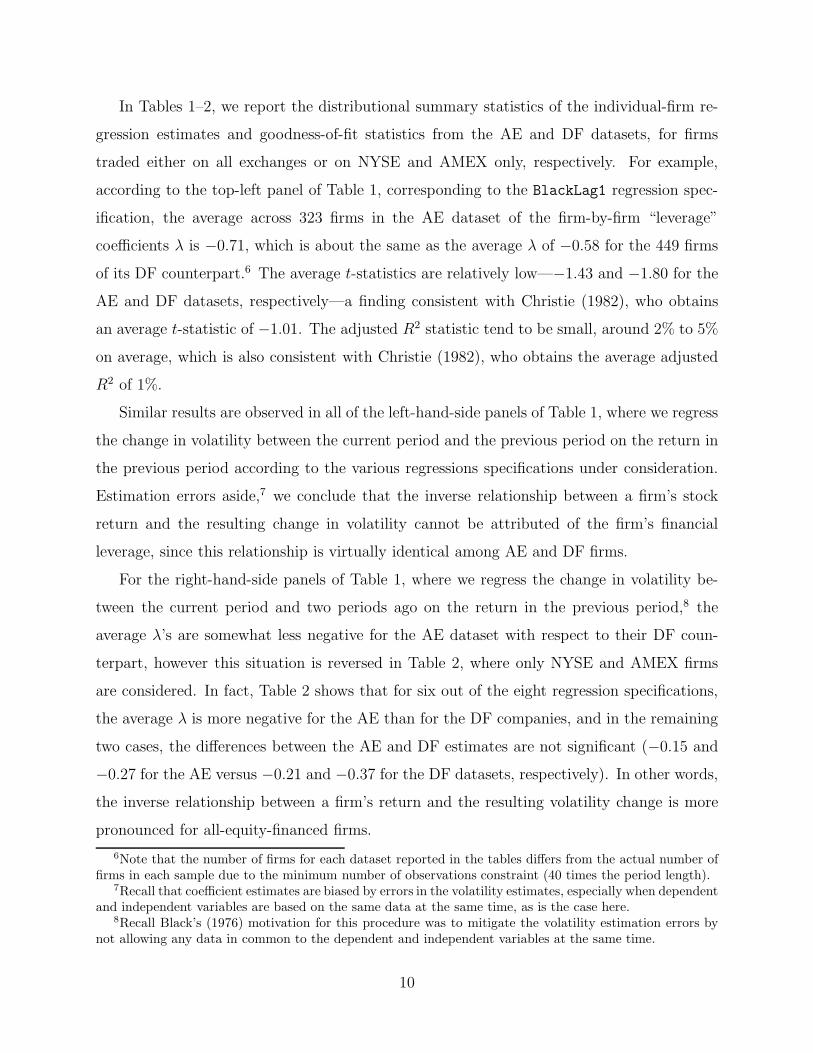
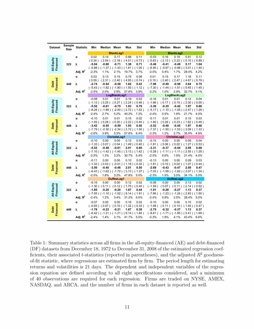
In Tables 1–2, we report the distributional summary statistics of the individual-firm re-

gression estimates and goodness-of-fit statistics from the AE and DF datasets, for firms

traded either on all exchanges or on NYSE and AMEX only, respectively. For example,

according to the top-left panel of Table 1, corresponding to the BlackLag1 regression spec-

ification, the average across 323 firms in the AE dataset of the firm-by-firm “leverage”

coefficients λ is −0.71, which is about the same as the average λ of −0.58 for the 449 firms

of its DF counterpart.6 The average t-statistics are relatively low—−1.43 and −1.80 for the

AE and DF datasets, respectively—a finding consistent with Christie (1982), who obtains

an average t-statistic of −1.01. The adjusted R2 statistic tend to be small, around 2% to 5%

on average, which is also consistent with Christie (1982), who obtains the average adjusted

R2 of 1%.

Similar results are observed in all of the left-hand-side panels of Table 1, where we regress

the change in volatility between the current period and the previous period on the return in

the previous period according to the various regressions specifications under consideration.

Estimation errors aside,7 we conclude that the inverse relationship between a firm’s stock

return and the resulting change in volatility cannot be attributed of the firm’s financial

leverage, since this relationship is virtually identical among AE and DF firms.

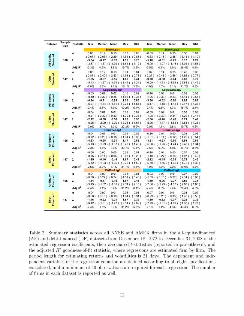
For the right-hand-side panels of Table 1, where we regress the change in volatility be-

tween the current period and two periods ago on the return in the previous period,8 the

average λ’s are somewhat less negative for the AE dataset with respect to their DF coun-

terpart, however this situation is reversed in Table 2, where only NYSE and AMEX firms

are considered. In fact, Table 2 shows that for six out of the eight regression specifications,

the average λ is more negative for the AE than for the DF companies, and in the remaining

two cases, the differences between the AE and DF estimates are not significant (−0.15 and

−0.27 for the AE versus −0.21 and −0.37 for the DF datasets, respectively). In other words,

the inverse relationship between a firm’s return and the resulting volatility change is more

pronounced for all-equity-financed firms.

6Note that the number of firms for each dataset reported in the tables differs from the actual number offirms in each sample due to the minimum number of observations constraint (40 times the period length).

7Recall that coefficient estimates are biased by errors in the volatility estimates, especially when dependentand independent variables are based on the same data at the same time, as is the case here.

8Recall Black’s (1976) motivation for this procedure was to mitigate the volatility estimation errors bynot allowing any data in common to the dependent and independent variables at the same time.

10

DatasetSample

SizeStatistic Min Median Mean Max Std Min Median Mean Max Std

α 0.02 0.14 0.17 0.88 0.11 -0.03 0.16 0.19 0.91 0.12

( 0.34 ) ( 2.04 ) ( 2.18 ) ( 4.51 ) ( 0.73 ) ( -0.63 ) ( 2.13 ) ( 2.22 ) ( 5.15 ) ( 0.89 )

λλλλ -5.04 -0.60 -0.71 1.38 0.71 -5.48 -0.41 -0.49 5.17 1.04

( -5.88 ) ( -1.37 ) ( -1.43 ) ( 1.81 ) ( 1.05 ) ( -6.95 ) ( -0.97 ) ( -0.98 ) ( 3.01 ) ( 1.40 )

Adj. R2

-2.3% 1.1% 2.1% 19.7% 3.7% -2.5% 0.4% 1.7% 28.4% 4.2%

α 0.03 0.13 0.15 0.75 0.08 0.01 0.15 0.17 1.16 0.11

( 0.55 ) ( 2.31 ) ( 2.40 ) ( 4.93 ) ( 0.74 ) ( 0.10 ) ( 2.40 ) ( 2.47 ) ( 4.67 ) ( 0.79 )

λλλλ -2.74 -0.54 -0.58 1.62 0.43 -7.98 -0.49 -0.58 3.64 0.75

( -5.43 ) ( -1.82 ) ( -1.80 ) ( 1.50 ) ( 1.12 ) ( -7.30 ) ( -1.44 ) ( -1.51 ) ( 5.45 ) ( 1.45 )

Adj. R2

-2.5% 2.0% 2.9% 27.6% 3.9% -2.2% 1.0% 2.9% 32.7% 5.1%

α -0.08 0.01 0.01 0.19 0.03 -0.16 0.01 0.01 0.12 0.04

( -1.13 ) ( 0.25 ) ( 0.27 ) ( 2.24 ) ( 0.46 ) ( -1.86 ) ( 0.17 ) ( 0.15 ) ( 2.30 ) ( 0.55 )

λλλλ -5.52 -0.61 -0.75 1.93 0.79 -3.36 -0.35 -0.42 1.97 0.68

( -8.28 ) ( -1.89 ) ( -2.00 ) ( 2.72 ) ( 1.52 ) ( -5.17 ) ( -1.10 ) ( -1.05 ) ( 2.47 ) ( 1.29 )

Adj. R2

-2.4% 2.7% 5.2% 40.2% 7.3% -2.4% 0.5% 1.8% 21.7% 4.0%

α -0.10 0.01 0.01 0.15 0.02 -0.11 0.01 0.01 0.15 0.03

( -1.05 ) ( 0.28 ) ( 0.30 ) ( 2.22 ) ( 0.40 ) ( -1.60 ) ( 0.26 ) ( 0.23 ) ( 1.62 ) ( 0.49 )

λλλλ -3.42 -0.55 -0.59 1.93 0.50 -2.52 -0.40 -0.45 1.97 0.46

( -7.79 ) ( -2.30 ) ( -2.34 ) ( 2.72 ) ( 1.50 ) ( -7.37 ) ( -1.50 ) ( -1.53 ) ( 3.09 ) ( 1.33 )

Adj. R2

-2.6% 3.9% 5.5% 57.6% 6.4% -2.3% 1.2% 2.7% 35.0% 4.8%

α -0.10 0.00 0.00 0.12 0.03 -0.15 0.00 0.00 0.09 0.04

( -1.33 ) ( 0.07 ) ( 0.04 ) ( 1.49 ) ( 0.40 ) ( -1.81 ) ( 0.06 ) ( 0.02 ) ( 1.27 ) ( 0.53 )

λλλλ -5.52 -0.48 -0.61 2.01 0.80 -3.31 -0.37 -0.44 2.09 0.68

( -7.10 ) ( -1.42 ) ( -1.45 ) ( 3.13 ) ( 1.42 ) ( -5.28 ) ( -1.11 ) ( -1.11 ) ( 2.55 ) ( 1.29 )

Adj. R2

-2.5% 1.3% 3.2% 30.7% 5.4% -2.5% 0.6% 1.9% 21.4% 4.0%

α -0.11 0.00 0.00 0.10 0.02 -0.13 0.00 0.00 0.09 0.03

( -1.33 ) ( 0.03 ) ( -0.01 ) ( 1.18 ) ( 0.32 ) ( -1.81 ) ( 0.10 ) ( 0.02 ) ( 1.07 ) ( 0.44 )

λλλλ -3.50 -0.40 -0.46 2.01 0.50 -2.69 -0.43 -0.47 2.09 0.47

( -6.43 ) ( -1.62 ) ( -1.72 ) ( 3.13 ) ( 1.37 ) ( -7.03 ) ( -1.59 ) ( -1.62 ) ( 3.07 ) ( 1.34 )

Adj. R2

-2.5% 1.8% 3.2% 47.8% 5.0% -2.3% 1.5% 3.0% 34.1% 5.0%

α -0.15 0.00 0.00 0.12 0.02 -0.08 0.00 0.00 0.13 0.02

( -1.30 ) ( 0.11 ) ( 0.12 ) ( 1.75 ) ( 0.40 ) ( -1.59 ) ( 0.07 ) ( 0.11 ) ( 2.14 ) ( 0.52 )

λλλλ -1.85 -0.20 -0.20 1.87 0.44 -1.91 -0.26 -0.27 1.13 0.37

( -7.55 ) ( -1.10 ) ( -1.02 ) ( 9.14 ) ( 1.91 ) ( -7.66 ) ( -1.23 ) ( -1.24 ) ( 2.83 ) ( 1.50 )

Adj. R2

-2.4% 1.2% 3.4% 31.2% 6.0% -2.4% 0.8% 2.5% 28.4% 5.0%

α -0.07 0.00 0.00 0.16 0.02 -0.10 0.00 0.00 0.10 0.02

( -0.93 ) ( 0.07 ) ( 0.10 ) ( 1.32 ) ( 0.33 ) ( -1.68 ) ( 0.11 ) ( 0.14 ) ( 1.40 ) ( 0.47 )

λλλλ -1.78 -0.22 -0.21 1.87 0.39 -2.75 -0.32 -0.37 1.13 0.37

( -6.42 ) ( -1.21 ) ( -1.21 ) ( 9.14 ) ( 1.84 ) ( -8.61 ) ( -1.71 ) ( -1.85 ) ( 5.41 ) ( 1.69 )

Adj. R2

-2.4% 1.4% 3.1% 41.7% 5.5% -2.3% 1.8% 4.1% 43.4% 6.6%

All-Equity

Financed

Debt

Financed

323

449

323

449

323

449

DuffeeLag1 DuffeeLag2

All-Equity

Financed

Debt

Financed

All-Equity

Financed

Debt

Financed

LogBlackLag1 LogBlackLag2

ChristieLag1 ChristieLag2

BlackLag1 BlackLag2All-Equity

Financed

Debt

Financed

323

449

Table 1: Summary statistics across all firms in the all-equity-financed (AE) and debt-financed(DF) datasets from December 18, 1972 to December 31, 2008 of the estimated regression coef-ficients, their associated t-statistics (reported in parentheses), and the adjusted R2 goodness-of-fit statistic, where regressions are estimated firm by firm. The period length for estimatingreturns and volatilities is 21 days. The dependent and independent variables of the regres-sion equation are defined according to all eight specifications considered, and a minimumof 40 observations are required for each regression. Firms are traded on NYSE, AMEX,NASDAQ, and ARCA, and the number of firms in each dataset is reported as well.

11

DatasetSample


α 0.03 0.12 0.13 0.33 0.06 -0.03 0.14 0.15 0.36 0.07

( 0.67 ) ( 2.06 ) ( 2.29 ) ( 4.51 ) ( 0.83 ) ( -0.63 ) ( 2.18 ) ( 2.38 ) ( 5.15 ) ( 1.10 )

λλλλ -3.34 -0.77 -0.82 1.12 0.73 -5.10 -0.51 -0.73 5.17 1.29

( -3.87 ) ( -1.37 ) ( -1.39 ) ( 1.81 ) ( 1.12 ) ( -6.95 ) ( -1.07 ) ( -1.16 ) ( 3.01 ) ( 1.53 )

Adj. R2

-2.3% 0.9% 1.8% 19.7% 3.5% -2.5% 0.5% 1.9% 28.4% 4.4%

α 0.05 0.12 0.13 0.31 0.04 0.02 0.14 0.15 0.42 0.06

( 0.87 ) ( 2.40 ) ( 2.43 ) ( 4.93 ) ( 0.73 ) ( 0.27 ) ( 2.46 ) ( 2.56 ) ( 4.52 ) ( 0.77 )

λλλλ -1.55 -0.57 -0.55 1.62 0.44 -3.70 -0.50 -0.64 0.86 0.70

( -5.43 ) ( -1.57 ) ( -1.74 ) ( 1.49 ) ( 1.24 ) ( -6.09 ) ( -1.53 ) ( -1.58 ) ( 2.84 ) ( 1.49 )

Adj. R2

-2.0% 1.6% 2.7% 15.1% 3.6% -1.9% 1.0% 3.1% 31.7% 5.6%

α -0.03 0.01 0.02 0.10 0.02 -0.10 0.01 0.01 0.08 0.03

( -0.40 ) ( 0.32 ) ( 0.35 ) ( 1.58 ) ( 0.35 ) ( -1.86 ) ( 0.33 ) ( 0.23 ) ( 1.41 ) ( 0.57 )

λλλλ -4.94 -0.71 -0.85 1.05 0.86 -3.36 -0.52 -0.60 1.92 0.83

( -6.27 ) ( -1.74 ) ( -1.81 ) ( 2.24 ) ( 1.54 ) ( -5.17 ) ( -1.18 ) ( -1.18 ) ( 2.47 ) ( 1.33 )

Adj. R2

-2.4% 2.3% 3.9% 40.2% 6.4% -2.4% 0.6% 1.7% 15.7% 3.4%

α -0.04 0.01 0.01 0.08 0.02 -0.09 0.02 0.01 0.08 0.03

( -0.51 ) ( 0.32 ) ( 0.33 ) ( 1.70 ) ( 0.36 ) ( -1.08 ) ( 0.39 ) ( 0.34 ) ( 1.29 ) ( 0.47 )

λλλλ -2.12 -0.58 -0.56 1.80 0.50 -2.06 -0.40 -0.48 0.71 0.48

( -6.25 ) ( -2.09 ) ( -2.20 ) ( 2.23 ) ( 1.65 ) ( -5.26 ) ( -1.47 ) ( -1.53 ) ( 1.83 ) ( 1.35 )

Adj. R2

-2.0% 3.4% 5.0% 27.3% 5.9% -2.0% 1.1% 2.6% 19.7% 4.5%

α -0.04 0.01 0.01 0.09 0.02 -0.10 0.01 0.00 0.08 0.03

( -0.72 ) ( 0.20 ) ( 0.18 ) ( 1.34 ) ( 0.33 ) ( -1.81 ) ( 0.14 ) ( 0.12 ) ( 1.22 ) ( 0.54 )

λλλλ -4.83 -0.58 -0.71 1.17 0.88 -3.31 -0.53 -0.60 1.93 0.81

( -5.13 ) ( -1.29 ) ( -1.37 ) ( 2.79 ) ( 1.49 ) ( -5.28 ) ( -1.26 ) ( -1.24 ) ( 2.48 ) ( 1.34 )

Adj. R2

-2.3% 1.1% 2.6% 30.7% 5.1% -2.5% 0.9% 1.8% 16.7% 3.5%

α -0.06 0.00 0.00 0.03 0.01 -0.10 0.01 0.00 0.07 0.03

( -0.75 ) ( 0.11 ) ( 0.06 ) ( 0.63 ) ( 0.28 ) ( -1.10 ) ( 0.27 ) ( 0.16 ) ( 1.07 ) ( 0.42 )

λλλλ -1.95 -0.46 -0.44 1.67 0.49 -2.12 -0.45 -0.51 0.73 0.46

( -5.12 ) ( -1.63 ) ( -1.66 ) ( 2.79 ) ( 1.50 ) ( -5.50 ) ( -1.56 ) ( -1.65 ) ( 1.72 ) ( 1.36 )

Adj. R2

-2.5% 2.0% 3.1% 21.7% 4.4% -1.9% 1.3% 2.9% 19.0% 4.5%

α -0.04 0.00 0.01 0.08 0.01 -0.03 0.00 0.01 0.07 0.02

( -0.86 ) ( 0.22 ) ( 0.24 ) ( 1.51 ) ( 0.40 ) ( -1.59 ) ( 0.15 ) ( 0.22 ) ( 2.14 ) ( 0.60 )

λλλλ -1.34 -0.17 -0.15 1.87 0.43 -1.39 -0.26 -0.27 0.59 0.34

( -5.45 ) ( -1.02 ) ( -1.01 ) ( 9.14 ) ( 2.15 ) ( -7.66 ) ( -1.23 ) ( -1.37 ) ( 2.60 ) ( 1.66 )

Adj. R2

-2.4% 1.1% 3.4% 31.2% 6.1% -2.4% 0.8% 2.4% 28.4% 4.6%

α -0.04 0.00 0.01 0.06 0.01 -0.07 0.01 0.01 0.08 0.02

( -0.68 ) ( 0.15 ) ( 0.19 ) ( 1.04 ) ( 0.34 ) ( -0.79 ) ( 0.26 ) ( 0.33 ) ( 1.40 ) ( 0.50 )

λλλλ -1.46 -0.22 -0.21 1.87 0.39 -1.30 -0.32 -0.37 0.22 0.32

( -6.42 ) ( -1.31 ) ( -1.27 ) ( 9.14 ) ( 2.02 ) ( -7.79 ) ( -1.81 ) ( -1.99 ) ( 1.36 ) ( 1.77 )

Adj. R2

-2.4% 1.6% 3.3% 31.2% 5.8% -2.1% 1.4% 4.3% 43.4% 6.9%



BlackLag1 BlackLag2


All-Equity

Financed

106

Debt

Financed

147

All-Equity

Financed

106

Debt

Financed

147

All-Equity

Financed

106

Debt

Financed

147

All-Equity

Financed

106

Debt

Financed

147

Table 2: Summary statistics across all NYSE and AMEX firms in the all-equity-financed(AE) and debt-financed (DF) datasets from December 18, 1972 to December 31, 2008 of theestimated regression coefficients, their associated t-statistics (reported in parentheses), andthe adjusted R2 goodness-of-fit statistic, where regressions are estimated firm by firm. Theperiod length for estimating returns and volatilities is 21 days. The dependent and inde-pendent variables of the regression equation are defined according to all eight specificationsconsidered, and a minimum of 40 observations are required for each regression. The numberof firms in each dataset is reported as well.

12

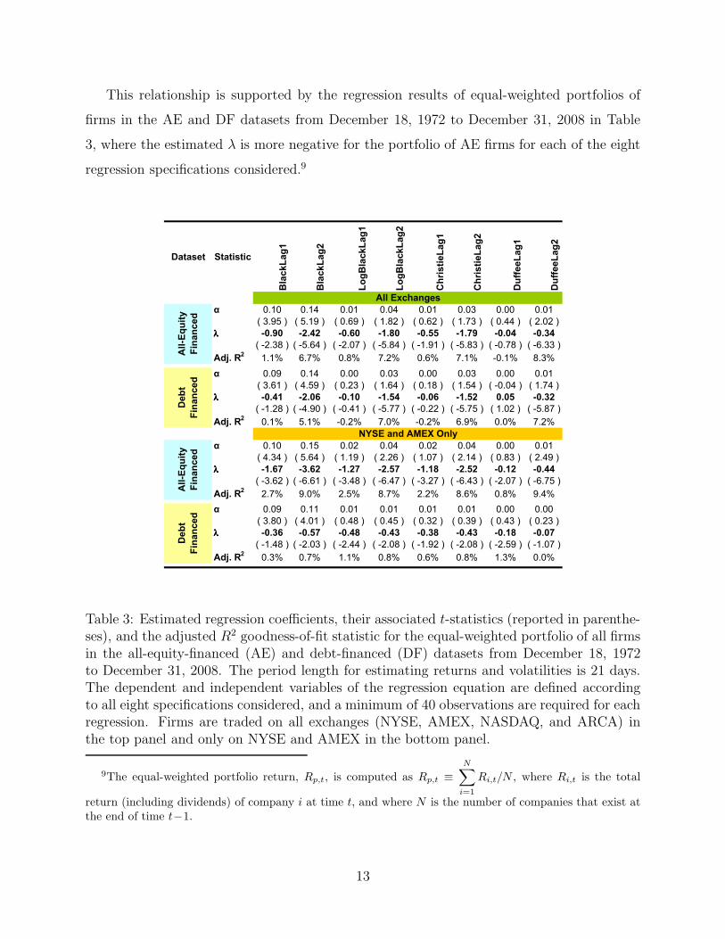
This relationship is supported by the regression results of equal-weighted portfolios of

firms in the AE and DF datasets from December 18, 1972 to December 31, 2008 in Table

3, where the estimated λ is more negative for the portfolio of AE firms for each of the eight

regression specifications considered.9

Dataset Statistic

BlackLag1

BlackLag2

LogBlackLag1

LogBlackLag2

ChristieLag1

ChristieLag2

DuffeeLag1

DuffeeLag2

α 0.10 0.14 0.01 0.04 0.01 0.03 0.00 0.01

( 3.95 ) ( 5.19 ) ( 0.69 ) ( 1.82 ) ( 0.62 ) ( 1.73 ) ( 0.44 ) ( 2.02 )

λλλλ -0.90 -2.42 -0.60 -1.80 -0.55 -1.79 -0.04 -0.34

( -2.38 ) ( -5.64 ) ( -2.07 ) ( -5.84 ) ( -1.91 ) ( -5.83 ) ( -0.78 ) ( -6.33 )

Adj. R2

1.1% 6.7% 0.8% 7.2% 0.6% 7.1% -0.1% 8.3%

α 0.09 0.14 0.00 0.03 0.00 0.03 0.00 0.01

( 3.61 ) ( 4.59 ) ( 0.23 ) ( 1.64 ) ( 0.18 ) ( 1.54 ) ( -0.04 ) ( 1.74 )

λλλλ -0.41 -2.06 -0.10 -1.54 -0.06 -1.52 0.05 -0.32

( -1.28 ) ( -4.90 ) ( -0.41 ) ( -5.77 ) ( -0.22 ) ( -5.75 ) ( 1.02 ) ( -5.87 )

Adj. R2

0.1% 5.1% -0.2% 7.0% -0.2% 6.9% 0.0% 7.2%

α 0.10 0.15 0.02 0.04 0.02 0.04 0.00 0.01

( 4.34 ) ( 5.64 ) ( 1.19 ) ( 2.26 ) ( 1.07 ) ( 2.14 ) ( 0.83 ) ( 2.49 )

λλλλ -1.67 -3.62 -1.27 -2.57 -1.18 -2.52 -0.12 -0.44

( -3.62 ) ( -6.61 ) ( -3.48 ) ( -6.47 ) ( -3.27 ) ( -6.43 ) ( -2.07 ) ( -6.75 )

Adj. R2

2.7% 9.0% 2.5% 8.7% 2.2% 8.6% 0.8% 9.4%

α 0.09 0.11 0.01 0.01 0.01 0.01 0.00 0.00

( 3.80 ) ( 4.01 ) ( 0.48 ) ( 0.45 ) ( 0.32 ) ( 0.39 ) ( 0.43 ) ( 0.23 )

λλλλ -0.36 -0.57 -0.48 -0.43 -0.38 -0.43 -0.18 -0.07

( -1.48 ) ( -2.03 ) ( -2.44 ) ( -2.08 ) ( -1.92 ) ( -2.08 ) ( -2.59 ) ( -1.07 )

Adj. R2

0.3% 0.7% 1.1% 0.8% 0.6% 0.8% 1.3% 0.0%

All Exchanges

All-Equity

Financed

Debt

Financed

NYSE and AMEX Only

All-Equity

Financed

Debt

Financed

Table 3: Estimated regression coefficients, their associated t-statistics (reported in parenthe-ses), and the adjusted R2 goodness-of-fit statistic for the equal-weighted portfolio of all firmsin the all-equity-financed (AE) and debt-financed (DF) datasets from December 18, 1972to December 31, 2008. The period length for estimating returns and volatilities is 21 days.The dependent and independent variables of the regression equation are defined accordingto all eight specifications considered, and a minimum of 40 observations are required for eachregression. Firms are traded on all exchanges (NYSE, AMEX, NASDAQ, and ARCA) inthe top panel and only on NYSE and AMEX in the bottom panel.

9The equal-weighted portfolio return, Rp,t, is computed as Rp,t ≡

N∑

i=1

Ri,t/N , where Ri,t is the total

return (including dividends) of company i at time t, and where N is the number of companies that exist atthe end of time t−1.

13

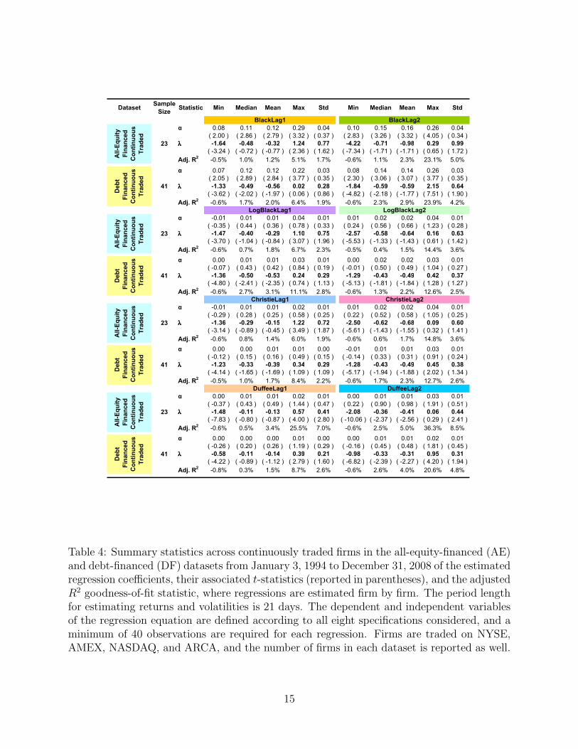
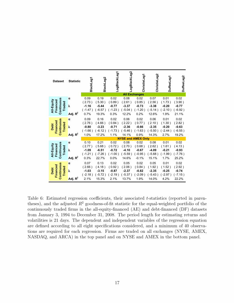
In Tables 4–6, we provide some robustness checks on our results by re-running the analysis

of Tables 1–3 for subsets of the AE and DF datasets containing only those firms that are

continuously traded over a common time period (see Duffee, 1995). And in Tables A.1–A.3

of the Appendix, we replicate the regressions of Table 1 but allow for more or less flexibility

in the estimates by focusing on the 10, 40, and 80-day volatility- and return-estimation

periods, respectively. All of these results are qualitatively consistent with the patterns from

the complete AE and DF samples.

5 Conclusion

The inverse relationship between equity returns and subsequent volatility changes is one of

the most well-established empirical regularities in stock-market data. Long considered to be

the result of leverage, the so-called “leverage effect” is, in fact, not due to leverage. Our

results show that this inverse relationship is at least as strong, and often stronger, among a

sample of all-equity-financed firms.

Our analysis does not provide a clear-cut alternative to the leverage explanation. By

ruling out leverage as the source of the return/volatility relationship, our results may be

interpreted as supportive of the time-varying expected return hypothesis of Pindyck (1984),

French, Schwert, and Stambaugh (1987), and Campbell and Hentschel (1992). Our findings

also support the recent volatility-feedback model of Danielsson, Shin, and Zigrand (2009),

in which asset-market volatility is endogenously determined in equilibrium by a combination

of leverage constraints, feedback effects, and market conditions.

However, our findings are also consistent with a behavioral interpretation in which in-

vestors’ behavior is shaped by their recent experiences, altering their perceptions of risk

and, consequently, giving rise to changes in their demand for risky assets. Such biased per-

ceptions of risk have been modeled by Gennaioli and Shleifer (2010), in which individuals

make judgments by recalling past experiences and scenarios that are the most representative

of the current situation, and combining these experiences with current information. Such

judgments will be biased not only because the representative scenarios that come to mind

depend on the situation being evaluated, but also because the scenarios that first come to

mind tend to be stereotypical ones. In our context, the first memories that come to mind

14

DatasetSample


α 0.08 0.11 0.12 0.29 0.04 0.10 0.15 0.16 0.26 0.04

( 2.00 ) ( 2.86 ) ( 2.79 ) ( 3.32 ) ( 0.37 ) ( 2.83 ) ( 3.26 ) ( 3.32 ) ( 4.05 ) ( 0.34 )

λλλλ -1.64 -0.48 -0.32 1.24 0.77 -4.22 -0.71 -0.98 0.29 0.99

( -3.24 ) ( -0.72 ) ( -0.77 ) ( 2.36 ) ( 1.62 ) ( -7.34 ) ( -1.71 ) ( -1.71 ) ( 0.65 ) ( 1.72 )

Adj. R2

-0.5% 1.0% 1.2% 5.1% 1.7% -0.6% 1.1% 2.3% 23.1% 5.0%

α 0.07 0.12 0.12 0.22 0.03 0.08 0.14 0.14 0.26 0.03

( 2.05 ) ( 2.89 ) ( 2.84 ) ( 3.77 ) ( 0.35 ) ( 2.30 ) ( 3.06 ) ( 3.07 ) ( 3.77 ) ( 0.35 )

λλλλ -1.33 -0.49 -0.56 0.02 0.28 -1.84 -0.59 -0.59 2.15 0.64

( -3.62 ) ( -2.02 ) ( -1.97 ) ( 0.06 ) ( 0.86 ) ( -4.82 ) ( -2.18 ) ( -1.77 ) ( 7.51 ) ( 1.90 )

Adj. R2

-0.6% 1.7% 2.0% 6.4% 1.9% -0.6% 2.3% 2.9% 23.9% 4.2%

α -0.01 0.01 0.01 0.04 0.01 0.01 0.02 0.02 0.04 0.01

( -0.35 ) ( 0.44 ) ( 0.36 ) ( 0.78 ) ( 0.33 ) ( 0.24 ) ( 0.56 ) ( 0.66 ) ( 1.23 ) ( 0.28 )

λλλλ -1.47 -0.40 -0.29 1.10 0.75 -2.57 -0.58 -0.64 0.16 0.63

( -3.70 ) ( -1.04 ) ( -0.84 ) ( 3.07 ) ( 1.96 ) ( -5.53 ) ( -1.33 ) ( -1.43 ) ( 0.61 ) ( 1.42 )

Adj. R2

-0.6% 0.7% 1.8% 6.7% 2.3% -0.5% 0.4% 1.5% 14.4% 3.6%

α 0.00 0.01 0.01 0.03 0.01 0.00 0.02 0.02 0.03 0.01

( -0.07 ) ( 0.43 ) ( 0.42 ) ( 0.84 ) ( 0.19 ) ( -0.01 ) ( 0.50 ) ( 0.49 ) ( 1.04 ) ( 0.27 )

λλλλ -1.36 -0.50 -0.53 0.24 0.29 -1.29 -0.43 -0.49 0.42 0.37

( -4.80 ) ( -2.41 ) ( -2.35 ) ( 0.74 ) ( 1.13 ) ( -5.13 ) ( -1.81 ) ( -1.84 ) ( 1.28 ) ( 1.27 )

Adj. R2

-0.6% 2.7% 3.1% 11.1% 2.8% -0.6% 1.3% 2.2% 12.6% 2.5%

α -0.01 0.01 0.01 0.02 0.01 0.01 0.02 0.02 0.04 0.01

( -0.29 ) ( 0.28 ) ( 0.25 ) ( 0.58 ) ( 0.25 ) ( 0.22 ) ( 0.52 ) ( 0.58 ) ( 1.05 ) ( 0.25 )

λλλλ -1.36 -0.29 -0.15 1.22 0.72 -2.50 -0.62 -0.68 0.09 0.60

( -3.14 ) ( -0.89 ) ( -0.45 ) ( 3.49 ) ( 1.87 ) ( -5.61 ) ( -1.43 ) ( -1.55 ) ( 0.32 ) ( 1.41 )

Adj. R2

-0.6% 0.8% 1.4% 6.0% 1.9% -0.6% 0.6% 1.7% 14.8% 3.6%

α 0.00 0.00 0.01 0.01 0.00 -0.01 0.01 0.01 0.03 0.01

( -0.12 ) ( 0.15 ) ( 0.16 ) ( 0.49 ) ( 0.15 ) ( -0.14 ) ( 0.33 ) ( 0.31 ) ( 0.91 ) ( 0.24 )

λλλλ -1.23 -0.33 -0.39 0.34 0.29 -1.28 -0.43 -0.49 0.45 0.38

( -4.14 ) ( -1.65 ) ( -1.69 ) ( 1.09 ) ( 1.09 ) ( -5.17 ) ( -1.94 ) ( -1.88 ) ( 2.02 ) ( 1.34 )

Adj. R2

-0.5% 1.0% 1.7% 8.4% 2.2% -0.6% 1.7% 2.3% 12.7% 2.6%

α 0.00 0.01 0.01 0.02 0.01 0.00 0.01 0.01 0.03 0.01

( -0.37 ) ( 0.43 ) ( 0.49 ) ( 1.44 ) ( 0.47 ) ( 0.22 ) ( 0.90 ) ( 0.98 ) ( 1.91 ) ( 0.51 )

λλλλ -1.48 -0.11 -0.13 0.57 0.41 -2.08 -0.36 -0.41 0.06 0.44

( -7.83 ) ( -0.80 ) ( -0.87 ) ( 4.00 ) ( 2.80 ) ( -10.06 ) ( -2.37 ) ( -2.56 ) ( 0.29 ) ( 2.41 )

Adj. R2

-0.6% 0.5% 3.4% 25.5% 7.0% -0.6% 2.5% 5.0% 36.3% 8.5%

α 0.00 0.00 0.00 0.01 0.00 0.00 0.01 0.01 0.02 0.01

( -0.26 ) ( 0.20 ) ( 0.26 ) ( 1.19 ) ( 0.29 ) ( -0.16 ) ( 0.45 ) ( 0.48 ) ( 1.81 ) ( 0.45 )

λλλλ -0.58 -0.11 -0.14 0.39 0.21 -0.98 -0.33 -0.31 0.95 0.31

( -4.22 ) ( -0.89 ) ( -1.12 ) ( 2.79 ) ( 1.60 ) ( -6.82 ) ( -2.39 ) ( -2.27 ) ( 4.20 ) ( 1.94 )

Adj. R2

-0.8% 0.3% 1.5% 8.7% 2.6% -0.6% 2.6% 4.0% 20.6% 4.8%

All-Equity

Financed

Continuous

Traded

23

Debt

Financed

Continuous

Traded

41


All-Equity

Financed

Continuous

Traded

23

Debt

Financed

Continuous

Traded

41

All-Equity

Financed

Continuous

Traded

23

Debt

Financed

Continuous

Traded

41



All-Equity

Financed

Continuous

Traded

Debt

Financed

Continuous

Traded

BlackLag1 BlackLag2

23

41

Table 4: Summary statistics across continuously traded firms in the all-equity-financed (AE)and debt-financed (DF) datasets from January 3, 1994 to December 31, 2008 of the estimatedregression coefficients, their associated t-statistics (reported in parentheses), and the adjustedR2 goodness-of-fit statistic, where regressions are estimated firm by firm. The period lengthfor estimating returns and volatilities is 21 days. The dependent and independent variablesof the regression equation are defined according to all eight specifications considered, and aminimum of 40 observations are required for each regression. Firms are traded on NYSE,AMEX, NASDAQ, and ARCA, and the number of firms in each dataset is reported as well.

15

DatasetSample


α 0.08 0.11 0.11 0.17 0.02 0.10 0.15 0.16 0.22 0.03

( 2.00 ) ( 2.85 ) ( 2.77 ) ( 3.32 ) ( 0.38 ) ( 2.83 ) ( 3.33 ) ( 3.35 ) ( 4.05 ) ( 0.36 )

λλλλ -1.64 -0.53 -0.29 1.24 0.82 -4.22 -1.00 -1.08 0.27 1.01

( -3.24 ) ( -0.70 ) ( -0.65 ) ( 2.36 ) ( 1.70 ) ( -7.34 ) ( -1.71 ) ( -1.83 ) ( 0.53 ) ( 1.77 )

Adj. R2

-0.5% 0.6% 1.2% 5.1% 1.8% -0.6% 1.1% 2.6% 23.1% 5.4%

α 0.07 0.12 0.12 0.16 0.03 0.08 0.14 0.14 0.21 0.03

( 2.39 ) ( 2.77 ) ( 2.81 ) ( 3.29 ) ( 0.25 ) ( 2.65 ) ( 3.21 ) ( 3.25 ) ( 3.77 ) ( 0.28 )

λλλλ -1.32 -0.56 -0.58 -0.29 0.26 -1.84 -0.97 -0.96 -0.36 0.41

( -2.96 ) ( -1.71 ) ( -1.78 ) ( -0.52 ) ( 0.76 ) ( -3.24 ) ( -2.79 ) ( -2.53 ) ( -1.14 ) ( 0.68 )

Adj. R2

-0.4% 1.4% 1.5% 4.2% 1.5% 0.2% 3.7% 3.2% 5.1% 1.7%

α -0.01 0.02 0.01 0.02 0.01 0.01 0.02 0.02 0.04 0.01

( -0.35 ) ( 0.47 ) ( 0.34 ) ( 0.78 ) ( 0.34 ) ( 0.24 ) ( 0.65 ) ( 0.69 ) ( 1.23 ) ( 0.28 )

λλλλ -1.47 -0.42 -0.25 1.10 0.79 -2.57 -0.61 -0.70 0.12 0.64

( -3.43 ) ( -0.90 ) ( -0.63 ) ( 3.07 ) ( 1.96 ) ( -5.53 ) ( -1.33 ) ( -1.53 ) ( 0.26 ) ( 1.45 )

Adj. R2

-0.6% 0.5% 1.7% 5.8% 2.1% -0.5% 0.4% 1.7% 14.4% 3.8%

α 0.00 0.01 0.01 0.02 0.00 0.01 0.02 0.02 0.03 0.01

( 0.11 ) ( 0.43 ) ( 0.42 ) ( 0.65 ) ( 0.13 ) ( 0.41 ) ( 0.64 ) ( 0.66 ) ( 1.04 ) ( 0.20 )

λλλλ -1.36 -0.50 -0.54 0.08 0.30 -1.29 -0.80 -0.73 -0.29 0.30

( -3.86 ) ( -2.20 ) ( -2.08 ) ( 0.19 ) ( 1.06 ) ( -3.31 ) ( -2.44 ) ( -2.39 ) ( -1.22 ) ( 0.66 )

Adj. R2

-0.6% 2.7% 2.4% 7.3% 2.3% 0.3% 2.7% 2.8% 5.4% 1.6%

α -0.01 0.01 0.01 0.02 0.01 0.01 0.02 0.02 0.04 0.01

( -0.29 ) ( 0.31 ) ( 0.25 ) ( 0.58 ) ( 0.26 ) ( 0.23 ) ( 0.57 ) ( 0.62 ) ( 1.05 ) ( 0.24 )

λλλλ -1.36 -0.30 -0.12 1.22 0.77 -2.50 -0.65 -0.74 0.06 0.61

( -3.14 ) ( -0.74 ) ( -0.30 ) ( 3.49 ) ( 1.93 ) ( -5.61 ) ( -1.44 ) ( -1.66 ) ( 0.14 ) ( 1.45 )

Adj. R2

-0.6% 0.6% 1.4% 6.0% 2.0% -0.6% 0.6% 1.9% 14.8% 3.9%

α 0.00 0.01 0.01 0.01 0.00 0.00 0.02 0.02 0.03 0.01

( -0.05 ) ( 0.24 ) ( 0.25 ) ( 0.49 ) ( 0.15 ) ( 0.03 ) ( 0.48 ) ( 0.49 ) ( 0.91 ) ( 0.24 )

λλλλ -1.23 -0.41 -0.42 0.28 0.31 -1.28 -0.82 -0.74 -0.31 0.29

( -3.47 ) ( -1.75 ) ( -1.63 ) ( 0.72 ) ( 1.04 ) ( -3.39 ) ( -2.47 ) ( -2.48 ) ( -1.30 ) ( 0.67 )

Adj. R2

-0.4% 1.2% 1.5% 5.9% 1.8% 0.4% 2.8% 3.1% 5.6% 1.7%

α 0.00 0.01 0.01 0.02 0.01 0.00 0.01 0.01 0.03 0.01

( -0.37 ) ( 0.56 ) ( 0.53 ) ( 1.44 ) ( 0.49 ) ( 0.24 ) ( 1.06 ) ( 1.08 ) ( 1.91 ) ( 0.48 )

λλλλ -1.48 -0.13 -0.14 0.57 0.44 -2.08 -0.39 -0.45 0.04 0.45

( -7.83 ) ( -0.81 ) ( -0.92 ) ( 4.00 ) ( 3.00 ) ( -10.06 ) ( -2.64 ) ( -2.78 ) ( 0.29 ) ( 2.49 )

Adj. R2

-0.5% 1.1% 3.9% 25.5% 7.3% -0.6% 3.3% 5.6% 36.3% 8.9%

α 0.00 0.00 0.01 0.01 0.00 0.00 0.01 0.01 0.02 0.01

( -0.02 ) ( 0.35 ) ( 0.44 ) ( 1.19 ) ( 0.35 ) ( -0.06 ) ( 0.69 ) ( 0.81 ) ( 1.81 ) ( 0.52 )

λλλλ -0.58 -0.17 -0.18 0.39 0.22 -0.98 -0.43 -0.46 -0.14 0.23

( -3.74 ) ( -1.22 ) ( -1.54 ) ( 2.26 ) ( 1.63 ) ( -5.54 ) ( -3.23 ) ( -3.30 ) ( -1.12 ) ( 1.46 )

Adj. R2

-0.8% 1.0% 2.1% 6.9% 2.8% 0.1% 5.1% 6.2% 14.4% 4.9%

BlackLag1 BlackLag2




All

-Eq

uit

y

Fin

an

ced

Co

nti

nu

ou

s

Tra

ded

20

Deb

t

Fin

an

ced

Co

nti

nu

ou

s

Tra

ded

15

All

-Eq

uit

y

Fin

an

ced

Co

nti

nu

ou

s

Tra

ded

20

Deb

t

Fin

an

ced

Co

nti

nu

ou

s

Tra

ded

15

All

-Eq

uit

y

Fin

an

ced

Co

nti

nu

ou

s

Tra

ded

20

Deb

t

Fin

an

ced

Co

nti

nu

ou

s

Tra

ded

15

All

-Eq

uit

y

Fin

an

ced

Co

nti

nu

ou

s

Tra

ded

20

Deb

t

Fin

an

ced

Co

nti

nu

ou

s

Tra

ded

15

Table 5: Summary statistics across continuously traded NYSE and AMEX firms in the all-equity-financed (AE) and debt-financed (DF) datasets from January 3, 1994 to December31, 2008 of the estimated regression coefficients, their associated t-statistics (reported inparentheses), and the adjusted R2 goodness-of-fit statistic, where regressions are estimatedfirm by firm. The period length for estimating returns and volatilities is 21 days. Thedependent and independent variables of the regression equation are defined according toall eight specifications considered, and a minimum of 40 observations are required for eachregression. The number of firms in each dataset is reported as well.

16

Dataset Statistic

BlackLag1

BlackLag2

LogBlackLag1

LogBlackLag2

ChristieLag1

ChristieLag2

DuffeeLag1

DuffeeLag2

α 0.09 0.19 0.02 0.08 0.02 0.07 0.01 0.02

( 2.73 ) ( 5.30 ) ( 0.89 ) ( 2.61 ) ( 0.85 ) ( 2.56 ) ( 1.73 ) ( 3.90 )

λλλλ -1.16 -5.44 -0.77 -3.37 -0.73 -3.38 -0.20 -0.77

( -1.47 ) ( -6.57 ) ( -1.23 ) ( -5.04 ) ( -1.20 ) ( -5.14 ) ( -2.10 ) ( -6.92 )

Adj. R2

0.7% 19.3% 0.3% 12.2% 0.2% 12.6% 1.9% 21.1%

α 0.09 0.16 0.02 0.06 0.02 0.06 0.01 0.02

( 2.76 ) ( 4.66 ) ( 0.84 ) ( 2.22 ) ( 0.77 ) ( 2.10 ) ( 1.30 ) ( 2.82 )

λλλλ -0.80 -3.23 -0.71 -2.36 -0.66 -2.35 -0.20 -0.63

( -1.66 ) ( -6.12 ) ( -1.73 ) ( -5.46 ) ( -1.63 ) ( -5.50 ) ( -2.44 ) ( -6.55 )

Adj. R2

1.0% 17.2% 1.1% 14.1% 0.9% 14.3% 2.7% 19.2%

α 0.10 0.21 0.02 0.08 0.02 0.08 0.01 0.02

( 2.77 ) ( 5.68 ) ( 0.72 ) ( 2.70 ) ( 0.68 ) ( 2.62 ) ( 1.61 ) ( 4.13 )

λλλλ -1.09 -6.51 -0.72 -4.10 -0.67 -4.09 -0.21 -0.93

( -1.21 ) ( -7.26 ) ( -1.00 ) ( -5.59 ) ( -0.95 ) ( -5.68 ) ( -1.99 ) ( -7.76 )

Adj. R2

0.3% 22.7% 0.0% 14.6% -0.1% 15.1% 1.7% 25.2%

α 0.07 0.13 0.02 0.05 0.02 0.05 0.01 0.02

( 2.66 ) ( 4.18 ) ( 0.92 ) ( 2.06 ) ( 0.84 ) ( 1.92 ) ( 1.52 ) ( 2.92 )

λλλλ -1.03 -3.15 -0.87 -2.37 -0.82 -2.35 -0.25 -0.74

( -2.18 ) ( -5.72 ) ( -2.19 ) ( -5.37 ) ( -2.09 ) ( -5.43 ) ( -2.97 ) ( -7.15 )

Adj. R2

2.1% 15.3% 2.1% 13.7% 1.9% 14.0% 4.2% 22.2%

All-Equity

Financed

Continuous

Traded

Debt

Financed

Continuous

Traded

All Exchanges

NYSE and AMEX Only

All-Equity

Financed

Continuous

Traded

Debt

Financed

Continuous

Traded

Table 6: Estimated regression coefficients, their associated t-statistics (reported in paren-theses), and the adjusted R2 goodness-of-fit statistic for the equal-weighted portfolio of thecontinuously traded firms in the all-equity-financed (AE) and debt-financed (DF) datasetsfrom January 3, 1994 to December 31, 2008. The period length for estimating returns andvolatilities is 21 days. The dependent and independent variables of the regression equationare defined according to all eight specifications considered, and a minimum of 40 observa-tions are required for each regression. Firms are traded on all exchanges (NYSE, AMEX,NASDAQ, and ARCA) in the top panel and on NYSE and AMEX in the bottom panel.

17

of an investor who has experienced significant financial loss is despair; as a result, emotions

take hold, prompting the investor to quickly reverse his positions, rather than continuing

with a given investment policy.

The view that our recent experiences can have substantial effects on our future behavior

is also backed by Lleras, Kawahara, and Levinthal (2009).10 In their research, Lleras and

his co-authors show that memories of past experiences affect the kinds of information we

pay attention to today. In particular, they compare the effects on the attention system of

externally-attributed rewards and penalties to the memory-driven effects that arise when

subjects repeatedly perform a task, and find that in both cases the attention system is

affected in analogous ways. This leads them to conclude that memories are tainted (positively

or negatively) by implicit assessments of our past performance.

Additional support for a behavioral interpretation of the leverage effect may be found

in some recent experimental evidence (Hens and Steude, 2009) in which 24 students were

asked to trade artificial securities with each other using an electronic trading system, and the

returns generated by these trades were negatively correlated with changes in future volatility

estimates. Clearly in this experimental context, neither leverage nor time-varying expected

returns can explain the inverse return/volatility relationship.

To distinguish among these competing explanations, further empirical and experimen-

tal analysis—with more explicit models of investor behavior and market equilibrium—is

required. We hope to pursue these extensions in future research.

10See also Lleras’ ongoing research as described in his APS Revolutionary Science 22nd Annual Conventioninvited talk “The Hidden Value In Memories: Equivalent Effects of Memory and External Rewards onAttention System” (May 2010).

18

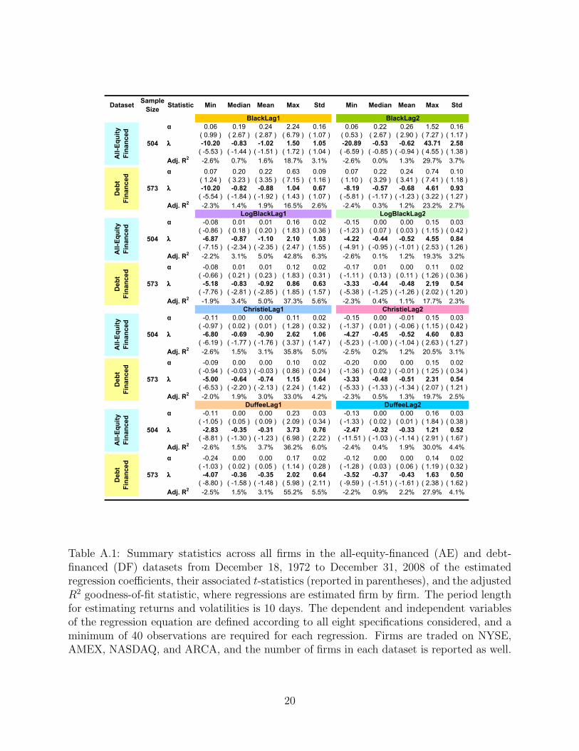
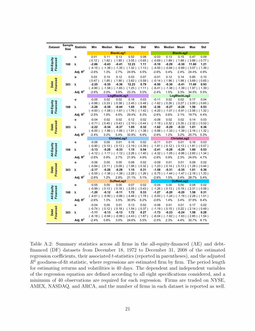
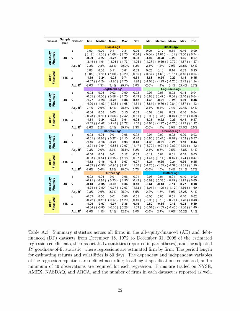
A Appendix

To provide additional robustness checks for our results, we re-run the analysis of Table 1 for

10, 40, and 80-day volatility- and return-estimation windows, and the results are reported

in Tables A.1–A.3, respectively. All of these results are qualitatively consistent with the

patterns from the complete AE and DF samples.

19

DatasetSample


α 0.06 0.19 0.24 2.24 0.16 0.06 0.22 0.26 1.52 0.16

( 0.99 ) ( 2.67 ) ( 2.87 ) ( 6.79 ) ( 1.07 ) ( 0.53 ) ( 2.67 ) ( 2.90 ) ( 7.27 ) ( 1.17 )

λλλλ -10.20 -0.83 -1.02 1.50 1.05 -20.89 -0.53 -0.62 43.71 2.58

( -5.53 ) ( -1.44 ) ( -1.51 ) ( 1.72 ) ( 1.04 ) ( -6.59 ) ( -0.85 ) ( -0.94 ) ( 4.55 ) ( 1.38 )

Adj. R2

-2.6% 0.7% 1.6% 18.7% 3.1% -2.6% 0.0% 1.3% 29.7% 3.7%

α 0.07 0.20 0.22 0.63 0.09 0.07 0.22 0.24 0.74 0.10

( 1.24 ) ( 3.23 ) ( 3.35 ) ( 7.15 ) ( 1.16 ) ( 1.10 ) ( 3.29 ) ( 3.41 ) ( 7.41 ) ( 1.18 )

λλλλ -10.20 -0.82 -0.88 1.04 0.67 -8.19 -0.57 -0.68 4.61 0.93

( -5.54 ) ( -1.84 ) ( -1.92 ) ( 1.43 ) ( 1.07 ) ( -5.81 ) ( -1.17 ) ( -1.23 ) ( 3.22 ) ( 1.27 )

Adj. R2

-2.3% 1.4% 1.9% 16.5% 2.6% -2.4% 0.3% 1.2% 23.2% 2.7%

α -0.08 0.01 0.01 0.16 0.02 -0.15 0.00 0.00 0.15 0.03

( -0.86 ) ( 0.18 ) ( 0.20 ) ( 1.83 ) ( 0.36 ) ( -1.23 ) ( 0.07 ) ( 0.03 ) ( 1.15 ) ( 0.42 )

λλλλ -6.87 -0.87 -1.10 2.10 1.03 -4.22 -0.44 -0.52 4.55 0.84

( -7.15 ) ( -2.34 ) ( -2.35 ) ( 2.47 ) ( 1.55 ) ( -4.91 ) ( -0.95 ) ( -1.01 ) ( 2.53 ) ( 1.26 )

Adj. R2

-2.2% 3.1% 5.0% 42.8% 6.3% -2.6% 0.1% 1.2% 19.3% 3.2%

α -0.08 0.01 0.01 0.12 0.02 -0.17 0.01 0.00 0.11 0.02

( -0.66 ) ( 0.21 ) ( 0.23 ) ( 1.83 ) ( 0.31 ) ( -1.11 ) ( 0.13 ) ( 0.11 ) ( 1.26 ) ( 0.36 )

λλλλ -5.18 -0.83 -0.92 0.86 0.63 -3.33 -0.44 -0.48 2.19 0.54

( -7.76 ) ( -2.81 ) ( -2.85 ) ( 1.85 ) ( 1.57 ) ( -5.38 ) ( -1.25 ) ( -1.26 ) ( 2.02 ) ( 1.20 )

Adj. R2

-1.9% 3.4% 5.0% 37.3% 5.6% -2.3% 0.4% 1.1% 17.7% 2.3%

α -0.11 0.00 0.00 0.11 0.02 -0.15 0.00 -0.01 0.15 0.03

( -0.97 ) ( 0.02 ) ( 0.01 ) ( 1.28 ) ( 0.32 ) ( -1.37 ) ( 0.01 ) ( -0.06 ) ( 1.15 ) ( 0.42 )

λλλλ -6.80 -0.69 -0.90 2.62 1.06 -4.27 -0.45 -0.52 4.60 0.83

( -6.19 ) ( -1.77 ) ( -1.76 ) ( 3.37 ) ( 1.47 ) ( -5.23 ) ( -1.00 ) ( -1.04 ) ( 2.63 ) ( 1.27 )

Adj. R2

-2.6% 1.5% 3.1% 35.8% 5.0% -2.5% 0.2% 1.2% 20.5% 3.1%

α -0.09 0.00 0.00 0.10 0.02 -0.20 0.00 0.00 0.15 0.02

( -0.94 ) ( -0.03 ) ( -0.03 ) ( 0.86 ) ( 0.24 ) ( -1.36 ) ( 0.02 ) ( -0.01 ) ( 1.25 ) ( 0.34 )

λλλλ -5.00 -0.64 -0.74 1.15 0.64 -3.33 -0.48 -0.51 2.31 0.54

( -6.53 ) ( -2.20 ) ( -2.13 ) ( 2.24 ) ( 1.42 ) ( -5.33 ) ( -1.33 ) ( -1.34 ) ( 2.07 ) ( 1.21 )

Adj. R2

-2.0% 1.9% 3.0% 33.0% 4.2% -2.3% 0.5% 1.3% 19.7% 2.5%

α -0.11 0.00 0.00 0.23 0.03 -0.13 0.00 0.00 0.16 0.03

( -1.05 ) ( 0.05 ) ( 0.09 ) ( 2.09 ) ( 0.34 ) ( -1.33 ) ( 0.02 ) ( 0.01 ) ( 1.84 ) ( 0.38 )

λλλλ -2.83 -0.35 -0.31 3.73 0.76 -2.47 -0.32 -0.33 1.21 0.52

( -8.81 ) ( -1.30 ) ( -1.23 ) ( 6.98 ) ( 2.22 ) ( -11.51 ) ( -1.03 ) ( -1.14 ) ( 2.91 ) ( 1.67 )

Adj. R2

-2.6% 1.5% 3.7% 36.2% 6.0% -2.4% 0.4% 1.9% 30.0% 4.4%

α -0.24 0.00 0.00 0.17 0.02 -0.12 0.00 0.00 0.14 0.02

( -1.03 ) ( 0.02 ) ( 0.05 ) ( 1.14 ) ( 0.28 ) ( -1.28 ) ( 0.03 ) ( 0.06 ) ( 1.19 ) ( 0.32 )

λλλλ -4.07 -0.36 -0.35 2.02 0.64 -3.52 -0.37 -0.43 1.63 0.50

( -8.80 ) ( -1.58 ) ( -1.48 ) ( 5.98 ) ( 2.11 ) ( -9.59 ) ( -1.51 ) ( -1.61 ) ( 2.38 ) ( 1.62 )

Adj. R2

-2.5% 1.5% 3.1% 55.2% 5.5% -2.2% 0.9% 2.2% 27.9% 4.1%



BlackLag1 BlackLag2


All

-Eq

uit

y

Fin

an

ced

504

Deb

t

Fin

an

ced

573

All

-Eq

uit

y

Fin

an

ced

504

Deb

t

Fin

an

ced

573

All

-Eq

uit

y

Fin

an

ced

504

Deb

t

Fin

an

ced

573

All

-Eq

uit

y

Fin

an

ced

504

Deb

t

Fin

an

ced

573

Table A.1: Summary statistics across all firms in the all-equity-financed (AE) and debt-financed (DF) datasets from December 18, 1972 to December 31, 2008 of the estimatedregression coefficients, their associated t-statistics (reported in parentheses), and the adjustedR2 goodness-of-fit statistic, where regressions are estimated firm by firm. The period lengthfor estimating returns and volatilities is 10 days. The dependent and independent variablesof the regression equation are defined according to all eight specifications considered, and aminimum of 40 observations are required for each regression. Firms are traded on NYSE,AMEX, NASDAQ, and ARCA, and the number of firms in each dataset is reported as well.

20

DatasetSample


α 0.01 0.11 0.13 0.52 0.08 -0.03 0.13 0.15 0.47 0.09

( 0.12 ) ( 1.82 ) ( 1.85 ) ( 3.55 ) ( 0.65 ) ( -0.69 ) ( 1.89 ) ( 1.88 ) ( 3.86 ) ( 0.77 )

λλλλ -2.86 -0.43 -0.41 12.23 1.11 -5.10 -0.29 -0.30 11.60 1.21

( -4.15 ) ( -1.38 ) ( -1.35 ) ( 1.32 ) ( 1.13 ) ( -4.50 ) ( -0.84 ) ( -0.89 ) ( 3.07 ) ( 1.39 )

Adj. R2

-2.6% 1.3% 2.7% 24.9% 4.5% -2.6% 0.4% 2.4% 24.4% 4.9%

α 0.03 0.10 0.12 0.53 0.07 -0.01 0.12 0.14 0.85 0.10

( 0.47 ) ( 1.85 ) ( 1.90 ) ( 3.83 ) ( 0.59 ) ( -0.14 ) ( 1.96 ) ( 1.98 ) ( 3.69 ) ( 0.65 )

λλλλ -2.25 -0.35 -0.36 12.23 0.79 -6.50 -0.36 -0.41 11.60 0.93

( -4.90 ) ( -1.58 ) ( -1.65 ) ( 1.25 ) ( 1.11 ) ( -6.41 ) ( -1.38 ) ( -1.39 ) ( 1.97 ) ( 1.39 )

Adj. R2

-2.6% 2.0% 3.5% 23.3% 5.0% -2.4% 1.5% 3.3% 34.5% 5.5%

α -0.05 0.02 0.02 0.18 0.03 -0.11 0.02 0.02 0.17 0.04

( -0.88 ) ( 0.33 ) ( 0.38 ) ( 2.45 ) ( 0.48 ) ( -1.62 ) ( 0.26 ) ( 0.27 ) ( 3.00 ) ( 0.65 )

λλλλ -3.28 -0.38 -0.44 1.05 0.55 -2.36 -0.27 -0.28 1.56 0.53

( -4.93 ) ( -1.58 ) ( -1.61 ) ( 1.76 ) ( 1.42 ) ( -4.20 ) ( -1.01 ) ( -0.91 ) ( 2.56 ) ( 1.32 )

Adj. R2

-2.5% 1.9% 4.5% 29.4% 6.3% -2.6% 0.6% 2.1% 19.7% 4.4%

α -0.04 0.02 0.02 0.12 0.02 -0.08 0.02 0.02 0.14 0.03

( -0.71 ) ( 0.40 ) ( 0.43 ) ( 2.10 ) ( 0.44 ) ( -1.18 ) ( 0.32 ) ( 0.35 ) ( 2.32 ) ( 0.52 )

λλλλ -2.22 -0.34 -0.37 1.05 0.32 -1.62 -0.29 -0.33 1.01 0.36

( -6.00 ) ( -1.86 ) ( -1.95 ) ( 1.91 ) ( 1.38 ) ( -5.88 ) ( -1.33 ) ( -1.39 ) ( 2.16 ) ( 1.32 )

Adj. R2

-2.4% 3.2% 5.4% 32.8% 6.9% -2.6% 1.2% 3.2% 25.7% 5.3%

α -0.06 0.00 0.01 0.16 0.02 -0.11 0.01 0.01 0.16 0.03

( -0.90 ) ( 0.10 ) ( 0.13 ) ( 2.19 ) ( 0.39 ) ( -1.81 ) ( 0.12 ) ( 0.13 ) ( 1.81 ) ( 0.57 )

λλλλ -3.13 -0.28 -0.33 1.15 0.54 -2.41 -0.28 -0.29 1.60 0.53

( -4.12 ) ( -1.11 ) ( -1.12 ) ( 2.26 ) ( 1.40 ) ( -4.32 ) ( -1.05 ) ( -0.96 ) ( 2.60 ) ( 1.34 )

Adj. R2

-2.6% 0.9% 2.7% 21.9% 4.9% -2.6% 0.9% 2.3% 24.0% 4.7%

α -0.06 0.00 0.00 0.08 0.02 -0.09 0.01 0.01 0.08 0.02

( -0.84 ) ( 0.11 ) ( 0.09 ) ( 1.06 ) ( 0.32 ) ( -1.23 ) ( 0.14 ) ( 0.13 ) ( 1.28 ) ( 0.44 )

λλλλ -2.17 -0.26 -0.28 1.15 0.31 -1.58 -0.31 -0.35 1.01 0.36

( -5.05 ) ( -1.36 ) ( -1.38 ) ( 2.28 ) ( 1.26 ) ( -5.75 ) ( -1.44 ) ( -1.47 ) ( 2.18 ) ( 1.33 )

Adj. R2

-2.6% 1.2% 2.9% 21.1% 5.1% -2.6% 1.5% 3.4% 28.7% 5.4%

α -0.05 0.00 0.00 0.07 0.02 -0.05 0.00 0.00 0.08 0.02

( -0.99 ) ( 0.13 ) ( 0.18 ) ( 2.05 ) ( 0.43 ) ( -1.26 ) ( 0.13 ) ( 0.19 ) ( 2.31 ) ( 0.59 )

λλλλ -1.20 -0.12 -0.11 1.72 0.33 -1.27 -0.20 -0.20 1.58 0.31

( -4.61 ) ( -0.90 ) ( -0.86 ) ( 4.48 ) ( 1.78 ) ( -5.93 ) ( -1.24 ) ( -1.19 ) ( 2.28 ) ( 1.51 )

Adj. R2

-2.6% 1.3% 3.5% 30.9% 6.2% -2.6% 1.4% 3.4% 37.9% 6.4%

α -0.04 0.00 0.01 0.13 0.02 -0.06 0.01 0.01 0.17 0.02

( -0.74 ) ( 0.12 ) ( 0.18 ) ( 1.54 ) ( 0.37 ) ( -1.19 ) ( 0.15 ) ( 0.22 ) ( 2.14 ) ( 0.49 )

λλλλ -1.11 -0.13 -0.13 1.72 0.27 -1.73 -0.23 -0.24 1.58 0.28

( -6.18 ) ( -0.94 ) ( -0.99 ) ( 4.43 ) ( 1.67 ) ( -6.04 ) ( -1.62 ) ( -1.63 ) ( 2.85 ) ( 1.54 )

Adj. R2

-2.4% 0.8% 3.0% 24.6% 5.5% -2.5% 2.3% 4.4% 30.7% 6.1%

All-Equity

Financed

168

Debt

Financed

303


All-Equity

Financed

168

Debt

Financed

303

All-Equity

Financed

168

Debt

Financed

303



Debt

Financed

303

BlackLag1 BlackLag2All-Equity

Financed

168


21

DatasetSample


α 0.00 0.09 0.11 0.31 0.06 0.00 0.12 0.14 0.46 0.09

( 0.12 ) ( 1.65 ) ( 1.68 ) ( 2.70 ) ( 0.54 ) ( 0.04 ) ( 1.81 ) ( 1.81 ) ( 3.50 ) ( 0.74 )

λλλλ -0.99 -0.27 -0.27 0.91 0.38 -1.97 -0.28 -0.29 1.65 0.67

( -3.44 ) ( -1.01 ) ( -1.03 ) ( 1.73 ) ( 1.25 ) ( -4.37 ) ( -0.69 ) ( -0.79 ) ( 1.87 ) ( 1.57 )

Adj. R2

-2.3% 0.8% 2.6% 20.9% 5.2% -2.5% 1.3% 2.9% 21.5% 5.4%

α 0.00 0.08 0.11 0.61 0.09 0.02 0.10 0.14 0.83 0.13

( 0.05 ) ( 1.56 ) ( 1.60 ) ( 3.20 ) ( 0.65 ) ( 0.34 ) ( 1.68 ) ( 1.67 ) ( 3.45 ) ( 0.64 )

λλλλ -1.59 -0.24 -0.24 0.71 0.31 -1.88 -0.24 -0.29 1.14 0.45

( -4.57 ) ( -1.24 ) ( -1.26 ) ( 1.75 ) ( 1.28 ) ( -4.08 ) ( -1.23 ) ( -1.20 ) ( 2.42 ) ( 1.24 )

Adj. R2

-2.6% 1.3% 3.4% 29.7% 6.0% -2.6% 1.1% 3.1% 27.4% 5.7%

α -0.03 0.03 0.03 0.09 0.02 -0.05 0.03 0.03 0.14 0.04

( -0.65 ) ( 0.60 ) ( 0.56 ) ( 1.70 ) ( 0.49 ) ( -0.83 ) ( 0.47 ) ( 0.54 ) ( 2.10 ) ( 0.64 )

λλλλ -1.27 -0.23 -0.28 0.86 0.42 -1.43 -0.21 -0.25 1.09 0.46

( -4.20 ) ( -1.03 ) ( -1.25 ) ( 1.68 ) ( 1.51 ) ( -3.84 ) ( -0.76 ) ( -0.84 ) ( 1.87 ) ( 1.43 )

Adj. R2

-2.1% 0.9% 4.4% 28.7% 7.5% -2.5% 0.5% 2.4% 22.4% 5.4%

α -0.04 0.03 0.03 0.15 0.03 -0.09 0.02 0.03 0.16 0.04

( -0.73 ) ( 0.50 ) ( 0.56 ) ( 2.42 ) ( 0.61 ) ( -0.98 ) ( 0.41 ) ( 0.46 ) ( 2.52 ) ( 0.58 )

λλλλ -1.61 -0.24 -0.22 0.61 0.28 -1.31 -0.22 -0.23 0.41 0.27

( -5.65 ) ( -1.42 ) ( -1.49 ) ( 1.77 ) ( 1.55 ) ( -3.98 ) ( -1.27 ) ( -1.25 ) ( 1.29 ) ( 1.17 )

Adj. R2

-2.6% 2.2% 5.1% 39.7% 8.3% -2.6% 1.4% 3.0% 24.5% 5.6%

α -0.03 0.01 0.01 0.06 0.02 -0.04 0.02 0.02 0.09 0.03

( -0.61 ) ( 0.26 ) ( 0.27 ) ( 1.10 ) ( 0.40 ) ( -0.86 ) ( 0.41 ) ( 0.40 ) ( 1.62 ) ( 0.57 )

λλλλ -1.16 -0.16 -0.20 0.93 0.40 -1.38 -0.21 -0.25 1.10 0.44

( -3.91 ) ( -0.64 ) ( -0.85 ) ( 2.07 ) ( 1.47 ) ( -3.79 ) ( -0.91 ) ( -0.89 ) ( 1.79 ) ( 1.42 )

Adj. R2

-2.3% 0.0% 2.9% 25.1% 6.2% -2.4% 0.8% 2.5% 16.8% 5.1%

α -0.06 0.01 0.01 0.12 0.02 -0.12 0.01 0.01 0.09 0.03

( -0.83 ) ( 0.14 ) ( 0.15 ) ( 1.18 ) ( 0.37 ) ( -1.47 ) ( 0.14 ) ( 0.15 ) ( 1.24 ) ( 0.47 )

λλλλ -1.52 -0.16 -0.15 0.67 0.27 -1.24 -0.25 -0.24 0.36 0.25

( -4.39 ) ( -0.96 ) ( -0.95 ) ( 2.01 ) ( 1.36 ) ( -4.78 ) ( -1.35 ) ( -1.32 ) ( 1.31 ) ( 1.20 )

Adj. R2

-2.6% 0.6% 2.6% 28.0% 5.7% -2.6% 1.5% 3.4% 24.1% 5.7%

α -0.02 0.01 0.01 0.06 0.01 -0.03 0.01 0.01 0.10 0.02

( -0.71 ) ( 0.28 ) ( 0.33 ) ( 1.55 ) ( 0.49 ) ( -0.82 ) ( 0.38 ) ( 0.49 ) ( 1.79 ) ( 0.65 )

λλλλ -0.40 -0.05 -0.08 0.36 0.18 -0.64 -0.13 -0.14 0.27 0.18

( -4.94 ) ( -0.50 ) ( -0.77 ) ( 2.63 ) ( 1.72 ) ( -5.04 ) ( -1.05 ) ( -1.12 ) ( 1.56 ) ( 1.60 )

Adj. R2

-2.3% 0.6% 3.7% 25.9% 6.5% -2.2% 1.5% 3.9% 35.2% 7.1%

α -0.03 0.00 0.01 0.06 0.01 -0.06 0.00 0.01 0.10 0.02

( -0.72 ) ( 0.12 ) ( 0.17 ) ( 1.20 ) ( 0.40 ) ( -0.95 ) ( 0.13 ) ( 0.21 ) ( 1.78 ) ( 0.48 )

λλλλ -1.00 -0.07 -0.07 0.36 0.19 -0.80 -0.14 -0.18 0.28 0.19

( -4.84 ) ( -0.80 ) ( -0.65 ) ( 3.28 ) ( 1.59 ) ( -5.04 ) ( -1.53 ) ( -1.45 ) ( 1.86 ) ( 1.40 )

Adj. R2

-2.6% 1.1% 3.1% 32.3% 6.0% -2.6% 2.7% 4.6% 35.2% 7.1%

All-Equity

Financed

48

Debt

Financed

115

All-Equity

Financed

48

Debt

Financed

115

All-Equity

Financed

48

Debt

Financed

115

All-Equity

Financed

48

Debt

Financed

115

BlackLag1 BlackLag2





22

References

Bekaert, G. and G. Wu, 2000, “Asymmetric Volatility and Risk in Equity Markets”, Review

of Financial Studies 13, 1–42.

Black, F., 1976, “Studies of Stock Price Volatility Changes”, Proceedings of the Business

and Economics Section of the American Statistical Association , 177–181.

Bollerslev, T., J. Litvinova, and G. Tauchen, 2006, “Leverage and Volatility Feedback Effects

in High-Frequency Data”, Journal of Financial Econometrics 4, 353–384.

Campbell, J. and L. Hentschel, 1992, “Non News is good news: An asymmetric model of

changing volatility in stock returns”, Journal of Financial Economics 31, 281–318.

Cheung, Y.-W. and L. Ng, 1992, “Stock Price Dynamics and Firm Size: An Empirical

Investigation”, Journal of Finance XLVII, 1985–1997.

Christie, A., 1982, “The Stochastic Behavior of Common Stock Variances: Value, leverage,

and Interest Rate Effects”, Journal of Financial Economics 10, 407–432.

Danielsson, J., H. S. Shin, and J.-P. Zigrand, 2009, “Risk Appetite and Endogenous Risk”,

Technical report, FRB of Cleveland/NBER Research Conference on Quantifying Systemic

Risk.

Duffee, G., 1995, “Stock Returns and Volatility: A Firm Level Analysis”, Journal of Finan-

cial Economics 37, 399–420.

Figlewski, S. and X. Wang, 2000, “Is the “Leverage Effect” a Leverage Effect?”, Technical

report, NYU Stern School of Business and City University of Hong Kong.

French, K., W. Schwert, and R. Stambaugh, 1987, “Expected Stock Returns and Volatility”,

Journal of Financial Economics 19, 3–29.

Gennaioli, N. and A. Shleifer, 2009, “What Comes to Mind”, Technical report, NBER Work-

ing Paper No. w15084.

Hens, T. and S. C. Steude, 2009, “The Leverage Effect Without Leverage”, Finance Research

Letters 6, 83–94.

Lleras, A., J. Kawahara, and B. R. Levinthal, 2009, “Past Rejections Lead to Future Misses:

Selection-Related Inhibition Produces Blink-Like Misses of Future (Easily Detectable)

Events”, Journal of Vision 9, 1–12.

Pindyck, R., 1984, “Risk, Inflation, and the Stock Market”, American Economic Review 74,

335–351.

Schwert, W., 1989, “Why Does Stock Market Volatility Change Over Time?”, Journal of

Finance XLIV, 1115–1153.

23

black’s leverage eﬀect is not due to...

Documents