biost 536 lecture 18 1 lecture 18 – multinomial and ordinal regression models
Post on 21-Dec-2015
273 views
TRANSCRIPT

BIOST 536 Lecture 18 1
Lecture 18 – Multinomial and Ordinal Regression Models Outcomes are discrete and on a nominal scale
1. Political party (Democrat, Republican, Green, Libertarian, etc.)
2. Religion
3. Disease type (No disease, cancer, CHD, etc.)
Ordering of categories is arbitrary
Model : Y = 0, 1, …, K (0 is the referent, but arbitrary)
Probability of being in a category depends on some covariate vector x
For simplicity, assume 3 outcome categories Y = 0, 1, 2
1 1 10 11 1 12 2 1 1
( 1| )logit (x) ( ) log ...
( 0 | ) p p
P Y xg x x x x
P Y x
2 2 20 21 1 22 2 2 2
( 2 | )logit (x) ( ) log ...
( 0 | ) p p
P Y xg x x x x
P Y x

BIOST 536 Lecture 18 2
Can compute the multinomial probability of being in each category
10 11 1 1 20 21 1 2 1 2... ...
1 1( 0 | )
1 1p p p px x x xP Y xe e e e
10 11 1 1 1
10 11 1 1 20 21 1 2 1 2
...
... ...( 1| )1 1
p p
p p p p
x x
x x x x
e eP Y x
e e e e
20 21 1 2 2
10 11 1 1 20 21 1 2 1 2
...
... ...( 2 | )1 1
p p
p p p p
x x
x x x x
e eP Y x
e e e e
Consider the relative risk ratio for outcome j relative to outcome 0 for comparing x=b to x=a
0 1
10 11 20 21 10 11 20 21
0 1
10 11 20 21 10 11 20 21
1( | ) ( 0 | ) 1 1( , )( | ) ( 0 | ) 1
1 1
j j
j j
a
a a a a
j b
b b b ab
eP Y j x a P Y x a e e e eRRR a bP Y j x b P Y x b e
e e e e
0 1
1
0 1
( )( , )j j
j
j j
aa b
j b
eRRR a b e
e
There are two relative risk ratios in this case for outcome 1 relative to 0 and outcome 2 relative to 0
comparing x=b to x=a
In some cases there may be value to testing 11 21
BIOST 536 Lecture 18 3
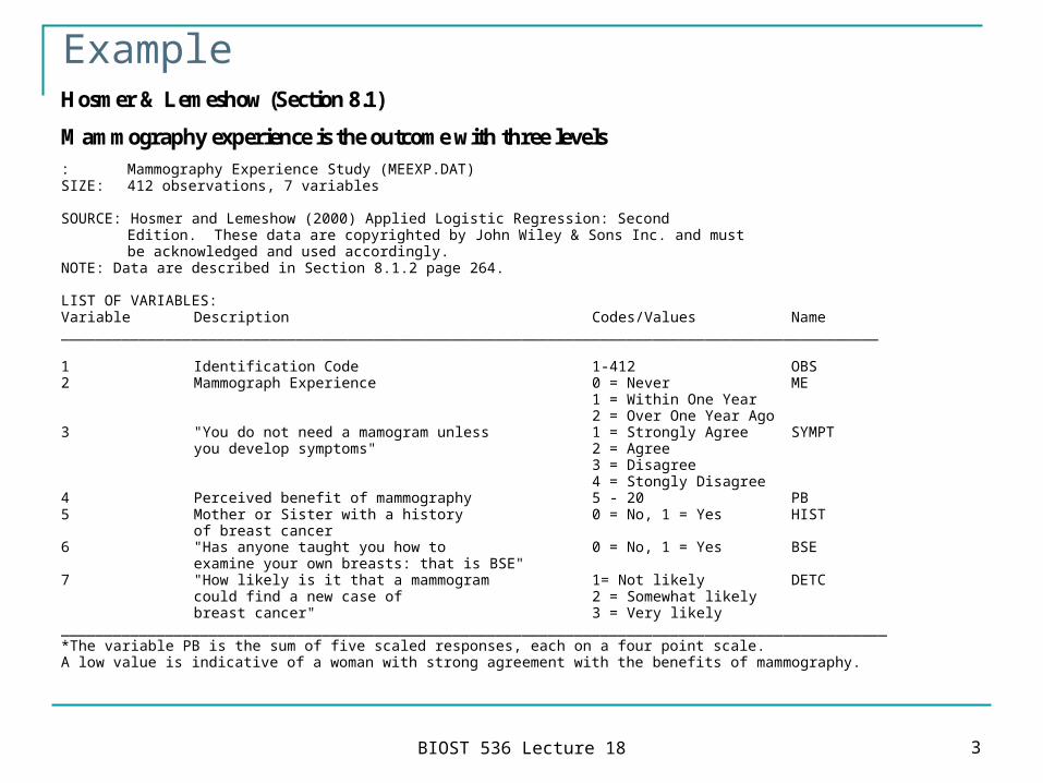
Example Hosmer & Lemeshow (Section 8.1)
Mammography experience is the outcome with three levels : Mammography Experience Study (MEEXP.DAT) SIZE: 412 observations, 7 variables SOURCE: Hosmer and Lemeshow (2000) Applied Logistic Regression: Second Edition. These data are copyrighted by John Wiley & Sons Inc. and must be acknowledged and used accordingly. NOTE: Data are described in Section 8.1.2 page 264. LIST OF VARIABLES: Variable Description Codes/Values Name ______________________________________________________________________________________________ 1 Identification Code 1-412 OBS 2 Mammograph Experience 0 = Never ME 1 = Within One Year 2 = Over One Year Ago 3 "You do not need a mamogram unless 1 = Strongly Agree SYMPT you develop symptoms" 2 = Agree 3 = Disagree 4 = Stongly Disagree 4 Perceived benefit of mammography 5 - 20 PB 5 Mother or Sister with a history 0 = No, 1 = Yes HIST of breast cancer 6 "Has anyone taught you how to 0 = No, 1 = Yes BSE examine your own breasts: that is BSE" 7 "How likely is it that a mammogram 1= Not likely DETC could find a new case of 2 = Somewhat likely breast cancer" 3 = Very likely _______________________________________________________________________________________________ *The variable PB is the sum of five scaled responses, each on a four point scale. A low value is indicative of a woman with strong agreement with the benefits of mammography.
BIOST 536 Lecture 18 4
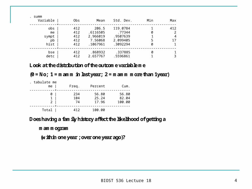
. summ Variable | Obs Mean Std. Dev. Min Max -------------+-------------------------------------------------------- obs | 412 206.5 119.0784 1 412 me | 412 .6116505 .77344 0 2 sympt | 412 2.966019 .9507639 1 4 pb | 412 7.56068 2.099405 5 17 hist | 412 .1067961 .3092294 0 1 -------------+-------------------------------------------------------- bse | 412 .868932 .337885 0 1 detc | 412 2.657767 .5596861 1 3
Look at the distribution of the outcome variable me
(0 = No; 1 = mamm in last year; 2 = mamm more than 1year) . tabulate me me | Freq. Percent Cum. ------------+----------------------------------- 0 | 234 56.80 56.80 1 | 104 25.24 82.04 2 | 74 17.96 100.00 ------------+----------------------------------- Total | 412 100.00
Does having a family history affect the likelihood of getting a
mammogram
(within one year ; over one year ago)?
BIOST 536 Lecture 18 5
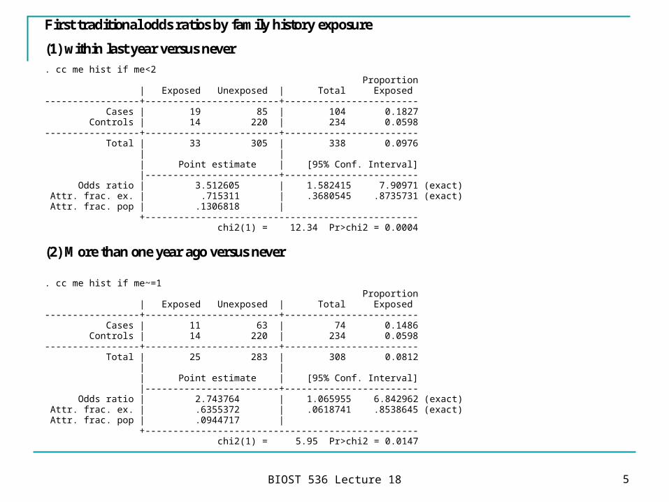
First traditional odds ratios by family history exposure
(1) within last year versus never . cc me hist if me<2 Proportion | Exposed Unexposed | Total Exposed -----------------+------------------------+------------------------ Cases | 19 85 | 104 0.1827 Controls | 14 220 | 234 0.0598 -----------------+------------------------+------------------------ Total | 33 305 | 338 0.0976 | | | Point estimate | [95% Conf. Interval] |------------------------+------------------------ Odds ratio | 3.512605 | 1.582415 7.90971 (exact) Attr. frac. ex. | .715311 | .3680545 .8735731 (exact) Attr. frac. pop | .1306818 | +------------------------------------------------- chi2(1) = 12.34 Pr>chi2 = 0.0004
(2) More than one year ago versus never . cc me hist if me~=1 Proportion | Exposed Unexposed | Total Exposed -----------------+------------------------+------------------------ Cases | 11 63 | 74 0.1486 Controls | 14 220 | 234 0.0598 -----------------+------------------------+------------------------ Total | 25 283 | 308 0.0812 | | | Point estimate | [95% Conf. Interval] |------------------------+------------------------ Odds ratio | 2.743764 | 1.065955 6.842962 (exact) Attr. frac. ex. | .6355372 | .0618741 .8538645 (exact) Attr. frac. pop | .0944717 | +------------------------------------------------- chi2(1) = 5.95 Pr>chi2 = 0.0147
BIOST 536 Lecture 18 6
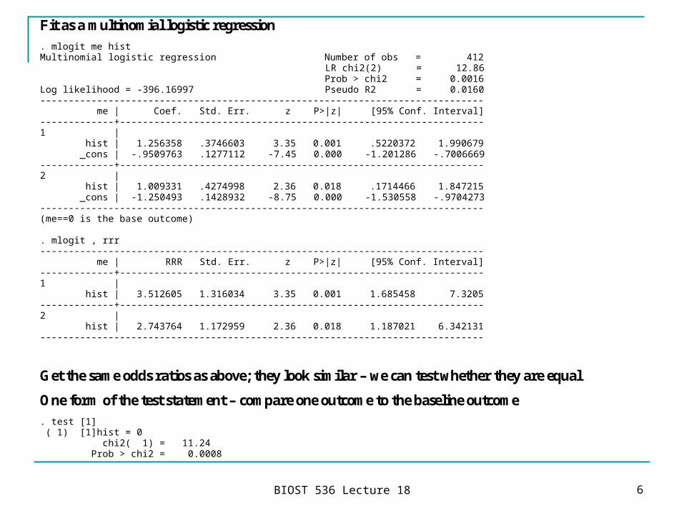
Fit as a multinomial logistic regression . mlogit me hist Multinomial logistic regression Number of obs = 412 LR chi2(2) = 12.86 Prob > chi2 = 0.0016 Log likelihood = -396.16997 Pseudo R2 = 0.0160 ------------------------------------------------------------------------------ me | Coef. Std. Err. z P>|z| [95% Conf. Interval] -------------+---------------------------------------------------------------- 1 | hist | 1.256358 .3746603 3.35 0.001 .5220372 1.990679 _cons | -.9509763 .1277112 -7.45 0.000 -1.201286 -.7006669 -------------+---------------------------------------------------------------- 2 | hist | 1.009331 .4274998 2.36 0.018 .1714466 1.847215 _cons | -1.250493 .1428932 -8.75 0.000 -1.530558 -.9704273 ------------------------------------------------------------------------------ (me==0 is the base outcome) . mlogit , rrr ------------------------------------------------------------------------------ me | RRR Std. Err. z P>|z| [95% Conf. Interval] -------------+---------------------------------------------------------------- 1 | hist | 3.512605 1.316034 3.35 0.001 1.685458 7.3205 -------------+---------------------------------------------------------------- 2 | hist | 2.743764 1.172959 2.36 0.018 1.187021 6.342131 ------------------------------------------------------------------------------
Get the same odds ratios as above; they look similar – we can test whether they are equal
One form of the test statement – compare one outcome to the baseline outcome . test [1] ( 1) [1]hist = 0 chi2( 1) = 11.24 Prob > chi2 = 0.0008
BIOST 536 Lecture 18 7
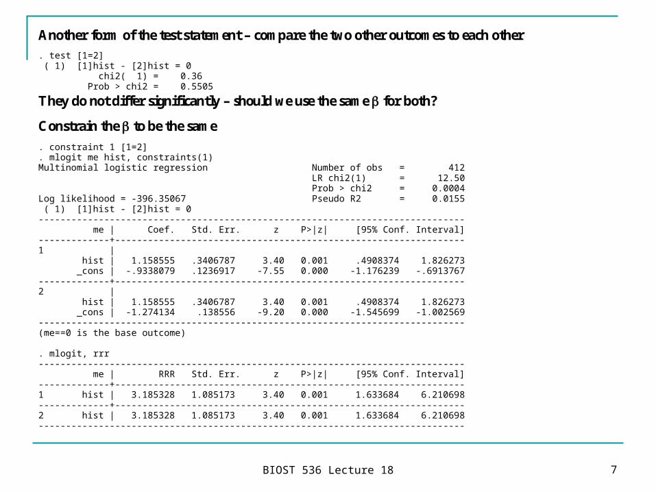
Another form of the test statement – compare the two other outcomes to each other . test [1=2] ( 1) [1]hist - [2]hist = 0 chi2( 1) = 0.36 Prob > chi2 = 0.5505
They do not differ significantly – should we use the same for both?
Constrain the to be the same
. constraint 1 [1=2]
. mlogit me hist, constraints(1) Multinomial logistic regression Number of obs = 412 LR chi2(1) = 12.50 Prob > chi2 = 0.0004 Log likelihood = -396.35067 Pseudo R2 = 0.0155 ( 1) [1]hist - [2]hist = 0 ------------------------------------------------------------------------------ me | Coef. Std. Err. z P>|z| [95% Conf. Interval] -------------+---------------------------------------------------------------- 1 | hist | 1.158555 .3406787 3.40 0.001 .4908374 1.826273 _cons | -.9338079 .1236917 -7.55 0.000 -1.176239 -.6913767 -------------+---------------------------------------------------------------- 2 | hist | 1.158555 .3406787 3.40 0.001 .4908374 1.826273 _cons | -1.274134 .138556 -9.20 0.000 -1.545699 -1.002569 ------------------------------------------------------------------------------ (me==0 is the base outcome) . mlogit, rrr ------------------------------------------------------------------------------ me | RRR Std. Err. z P>|z| [95% Conf. Interval] -------------+---------------------------------------------------------------- 1 hist | 3.185328 1.085173 3.40 0.001 1.633684 6.210698 -------------+---------------------------------------------------------------- 2 hist | 3.185328 1.085173 3.40 0.001 1.633684 6.210698 ------------------------------------------------------------------------------
BIOST 536 Lecture 18 8
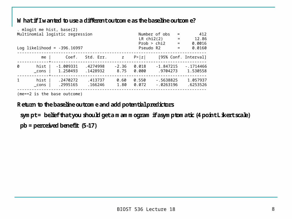
What if I wanted to use a different outcome as the baseline outcome? . mlogit me hist, base(2) Multinomial logistic regression Number of obs = 412 LR chi2(2) = 12.86 Prob > chi2 = 0.0016 Log likelihood = -396.16997 Pseudo R2 = 0.0160 ------------------------------------------------------------------------------ me | Coef. Std. Err. z P>|z| [95% Conf. Interval] -------------+---------------------------------------------------------------- 0 hist | -1.009331 .4274998 -2.36 0.018 -1.847215 -.1714466 _cons | 1.250493 .1428932 8.75 0.000 .9704273 1.530558 -------------+---------------------------------------------------------------- 1 hist | .2470272 .413737 0.60 0.550 -.5638825 1.057937 _cons | .2995165 .166246 1.80 0.072 -.0263196 .6253526 ------------------------------------------------------------------------------ (me==2 is the base outcome)
Return to the baseline outcome and add potential predictors
sympt = belief that you should get a mammogram if asymptomatic (4 point Likert scale)
pb = perceived benefit (5-17)

BIOST 536 Lecture 18 9
. mlogit me hist sympt pb Multinomial logistic regression Number of obs = 412 LR chi2(6) = 86.82 Prob > chi2 = 0.0000 Log likelihood = -359.18891 Pseudo R2 = 0.1078 ------------------------------------------------------------------------------ me | Coef. Std. Err. z P>|z| [95% Conf. Interval] -------------+---------------------------------------------------------------- 1 hist | 1.332345 .4121394 3.23 0.001 .5245667 2.140123 sympt | .9350847 .1710481 5.47 0.000 .5998365 1.270333 pb | -.2630025 .0716593 -3.67 0.000 -.4034522 -.1225527 _cons | -1.933438 .8388576 -2.30 0.021 -3.577568 -.289307 -------------+---------------------------------------------------------------- 2 hist | 1.039386 .4410652 2.36 0.018 .1749146 1.903858 sympt | .5279655 .1614014 3.27 0.001 .2116246 .8443063 pb | -.1601409 .0711738 -2.25 0.024 -.299639 -.0206429 _cons | -1.586551 .8054184 -1.97 0.049 -3.165142 -.0079599 ------------------------------------------------------------------------------ (me==0 is the base outcome)
Test whether the coefficients are the same between the two other outcomes . test [1==2] ( 1) [1]hist - [2]hist = 0 ( 2) [1]sympt - [2]sympt = 0 ( 3) [1]pb - [2]pb = 0 chi2( 3) = 7.25 Prob > chi2 = 0.0645
Simultaneous test of difference between all three covariates – may only want to test one . test [1==2]: hist ( 1) [1]hist - [2]hist = 0 chi2( 1) = 0.48 Prob > chi2 = 0.4866
BIOST 536 Lecture 18 10
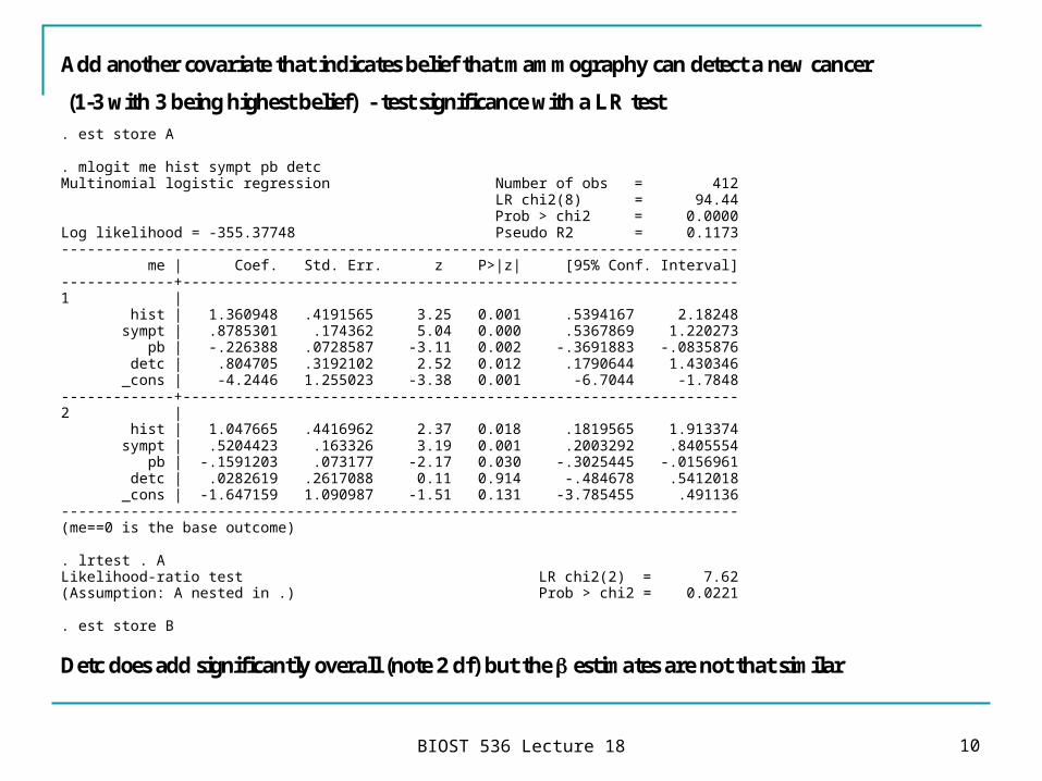
Add another covariate that indicates belief that mammography can detect a new cancer
(1-3 with 3 being highest belief) - test significance with a LR test . est store A . mlogit me hist sympt pb detc Multinomial logistic regression Number of obs = 412 LR chi2(8) = 94.44 Prob > chi2 = 0.0000 Log likelihood = -355.37748 Pseudo R2 = 0.1173 ------------------------------------------------------------------------------ me | Coef. Std. Err. z P>|z| [95% Conf. Interval] -------------+---------------------------------------------------------------- 1 | hist | 1.360948 .4191565 3.25 0.001 .5394167 2.18248 sympt | .8785301 .174362 5.04 0.000 .5367869 1.220273 pb | -.226388 .0728587 -3.11 0.002 -.3691883 -.0835876 detc | .804705 .3192102 2.52 0.012 .1790644 1.430346 _cons | -4.2446 1.255023 -3.38 0.001 -6.7044 -1.7848 -------------+---------------------------------------------------------------- 2 | hist | 1.047665 .4416962 2.37 0.018 .1819565 1.913374 sympt | .5204423 .163326 3.19 0.001 .2003292 .8405554 pb | -.1591203 .073177 -2.17 0.030 -.3025445 -.0156961 detc | .0282619 .2617088 0.11 0.914 -.484678 .5412018 _cons | -1.647159 1.090987 -1.51 0.131 -3.785455 .491136 ------------------------------------------------------------------------------ (me==0 is the base outcome) . lrtest . A Likelihood-ratio test LR chi2(2) = 7.62 (Assumption: A nested in .) Prob > chi2 = 0.0221 . est store B
Detc does add significantly overall (note 2 df) but the estimates are not that similar
BIOST 536 Lecture 18 11
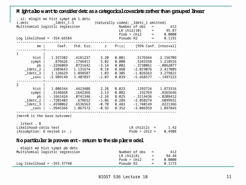
Might also want to consider detc as a categorical covariate rather than grouped linear . xi: mlogit me hist sympt pb i.detc i.detc _Idetc_1-3 (naturally coded; _Idetc_1 omitted) Multinomial logistic regression Number of obs = 412 LR chi2(10) = 95.87 Prob > chi2 = 0.0000 Log likelihood = -354.66584 Pseudo R2 = 0.1191 ------------------------------------------------------------------------------ me | Coef. Std. Err. z P>|z| [95% Conf. Interval] -------------+---------------------------------------------------------------- 1 | hist | 1.337202 .4181237 3.20 0.001 .5176944 2.156709 sympt | .876626 .1746411 5.02 0.000 .5343358 1.218916 pb | -.2296069 .0731642 -3.14 0.002 -.3730061 -.0862077 _Idetc_2 | .1989643 1.131674 0.18 0.860 -2.019076 2.417005 _Idetc_3 | 1.126629 1.098587 1.03 0.305 -1.026563 3.279821 _cons | -2.909149 1.407897 -2.07 0.039 -5.668577 -.1497223 -------------+---------------------------------------------------------------- 2 | hist | 1.006344 .4423408 2.28 0.023 .1393724 1.873316 sympt | .5146668 .1642366 3.13 0.002 .192769 .8365646 pb | -.1661424 .0741346 -2.24 0.025 -.3114436 -.0208412 _Idetc_2 | -.7201403 .678652 -1.06 0.289 -2.050274 .6099931 _Idetc_3 | -.4590062 .6536563 -0.70 0.483 -1.740149 .8221366 _cons | -.9945566 1.067572 -0.93 0.352 -3.086959 1.097845 ------------------------------------------------------------------------------ (me==0 is the base outcome) . lrtest . B Likelihood-ratio test LR chi2(2) = 1.42 (Assumption: B nested in .) Prob > chi2 = 0.4908
No particular improvement – return to the simpler model . mlogit me hist sympt pb detc Multinomial logistic regression Number of obs = 412 LR chi2(8) = 94.44 Prob > chi2 = 0.0000 Log likelihood = -355.37748 Pseudo R2 = 0.1173
BIOST 536 Lecture 18 12
------------------------------------------------------------------------------ me | Coef. Std. Err. z P>|z| [95% Conf. Interval] -------------+---------------------------------------------------------------- 1 | hist | 1.360948 .4191565 3.25 0.001 .5394167 2.18248 sympt | .8785301 .174362 5.04 0.000 .5367869 1.220273 pb | -.226388 .0728587 -3.11 0.002 -.3691883 -.0835876 detc | .804705 .3192102 2.52 0.012 .1790644 1.430346 _cons | -4.2446 1.255023 -3.38 0.001 -6.7044 -1.7848 -------------+---------------------------------------------------------------- 2 | hist | 1.047665 .4416962 2.37 0.018 .1819565 1.913374 sympt | .5204423 .163326 3.19 0.001 .2003292 .8405554 pb | -.1591203 .073177 -2.17 0.030 -.3025445 -.0156961 detc | .0282619 .2617088 0.11 0.914 -.484678 .5412018 _cons | -1.647159 1.090987 -1.51 0.131 -3.785455 .491136 ------------------------------------------------------------------------------ (me==0 is the base outcome)
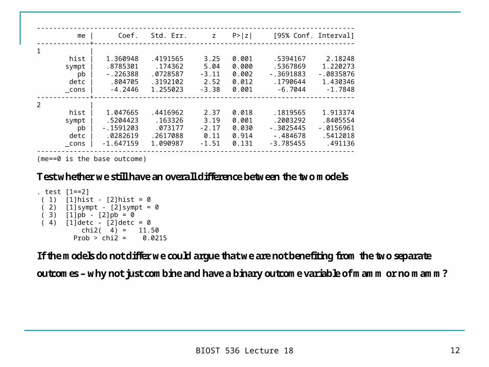
Test whether we still have an overall difference between the two models . test [1==2] ( 1) [1]hist - [2]hist = 0 ( 2) [1]sympt - [2]sympt = 0 ( 3) [1]pb - [2]pb = 0 ( 4) [1]detc - [2]detc = 0 chi2( 4) = 11.50 Prob > chi2 = 0.0215
If the models do not differ we could argue that we are not benefiting from the two separate
outcomes – why not just combine and have a binary outcome variable of mamm or no mamm?
BIOST 536 Lecture 18 13
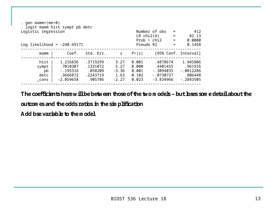
. gen mamm=(me>0)
. logit mamm hist sympt pb detc Logistic regression Number of obs = 412 LR chi2(4) = 82.13 Prob > chi2 = 0.0000 Log likelihood = -240.69171 Pseudo R2 = 0.1458 ------------------------------------------------------------------------------ mamm | Coef. Std. Err. z P>|z| [95% Conf. Interval] -------------+---------------------------------------------------------------- hist | 1.216836 .3719299 3.27 0.001 .4878674 1.945806 sympt | .7010307 .1331072 5.27 0.000 .4401455 .961916 pb | -.195316 .058209 -3.36 0.001 -.3094035 -.0812286 detc | .3666872 .2243719 1.63 0.102 -.0730737 .806448 _cons | -2.059658 .905786 -2.27 0.023 -3.834966 -.2843505 ------------------------------------------------------------------------------
The coefficients here will be between those of the two models – but loses some detail about the
outcomes and the odds ratios in the simplification
Add bse variable to the model
BIOST 536 Lecture 18 14
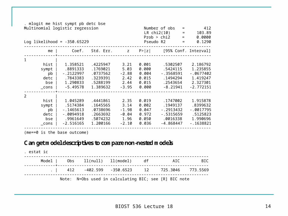
. mlogit me hist sympt pb detc bse Multinomial logistic regression Number of obs = 412 LR chi2(10) = 103.89 Prob > chi2 = 0.0000 Log likelihood = -350.65229 Pseudo R2 = 0.1290 ------------------------------------------------------------------------------ me | Coef. Std. Err. z P>|z| [95% Conf. Interval] -------------+---------------------------------------------------------------- 1 | hist | 1.358521 .4225947 3.21 0.001 .5302507 2.186792 sympt | .8891333 .1769021 5.03 0.000 .5424115 1.235855 pb | -.2122997 .0737562 -2.88 0.004 -.3568591 -.0677402 detc | .7843383 .3239391 2.42 0.015 .1494294 1.419247 bse | 1.290833 .5288199 2.44 0.015 .2543654 2.327301 _cons | -5.49578 1.389632 -3.95 0.000 -8.21941 -2.772151 -------------+---------------------------------------------------------------- 2 | hist | 1.045289 .4441861 2.35 0.019 .1747002 1.915878 sympt | .5174384 .1645565 3.14 0.002 .1949137 .8399632 pb | -.1465613 .0738696 -1.98 0.047 -.2913432 -.0017795 detc | -.0094918 .2663692 -0.04 0.972 -.5315659 .5125823 bse | .9961649 .5074232 1.96 0.050 .0016338 1.990696 _cons | -2.516165 1.200166 -2.10 0.036 -4.868447 -.1638821 ------------------------------------------------------------------------------ (me==0 is the base outcome)
Can get model descriptives to compare non-nested models . estat ic ----------------------------------------------------------------------------- Model | Obs ll(null) ll(model) df AIC BIC -------------+--------------------------------------------------------------- . | 412 -402.599 -350.6523 12 725.3046 773.5569 ----------------------------------------------------------------------------- Note: N=Obs used in calculating BIC; see [R] BIC note
BIOST 536 Lecture 18 15
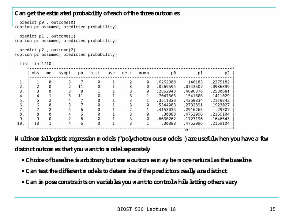
Can get the estimated probability of each of the three outcomes . predict p0 , outcome(0) (option pr assumed; predicted probability) . predict p1 , outcome(1) (option pr assumed; predicted probability) . predict p2 , outcome(2) (option pr assumed; predicted probability) . list in 1/10 +-----------------------------------------------------------------------------------+ | obs me sympt pb hist bse detc mamm p0 p1 p2 | |-----------------------------------------------------------------------------------| 1. | 1 0 3 7 0 1 2 0 .6262988 .146183 .2275182 | 2. | 2 0 2 11 0 1 3 0 .8269594 .0743507 .0986899 | 3. | 3 0 3 8 1 1 3 0 .2862943 .4606376 .2530681 | 4. | 4 1 3 11 0 1 3 1 .7047365 .1541606 .1411029 | 5. | 5 2 4 7 0 1 3 1 .3511323 .4368834 .2119843 | 6. | 6 0 3 7 0 1 3 0 .5344083 .2732891 .1923027 | 7. | 7 2 4 6 0 1 2 1 .4153034 .2916265 .29307 | 8. | 8 0 4 6 0 1 3 0 .30888 .4752096 .2159104 | 9. | 9 0 2 6 0 1 3 0 .6630262 .1723196 .1646543 | 10. | 10 1 4 6 0 1 3 1 .30888 .4752096 .2159104 | +-----------------------------------------------------------------------------------+
Multinomial logistic regression models (“polychotomous models”) are useful when you have a few
distinct outcomes that you want to model separately
Choice of baseline is arbitrary but some outcomes may be more natural as the baseline
Can test the different models to determine if the predictors really are distinct
Can impose constraints on variables you want to control while letting others vary
BIOST 536 Lecture 18 16
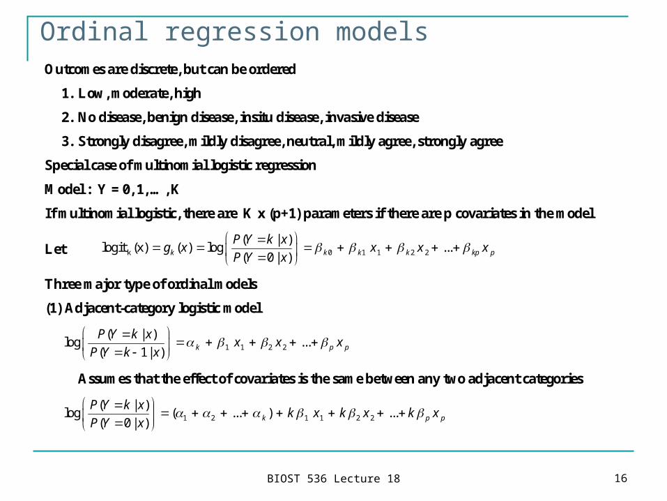
Ordinal regression models Outcomes are discrete, but can be ordered
1. Low, moderate, high
2. No disease, benign disease, insitu disease, invasive disease
3. Strongly disagree, mildly disagree, neutral, mildly agree, strongly agree
Special case of multinomial logistic regression
Model : Y = 0, 1, …, K
If multinomial logistic, there are K x (p+1) parameters if there are p covariates in the model
Let k 0 1 1 2 2
( | )logit (x) ( ) log ...
( 0 | )k k k k kp p
P Y k xg x x x x
P Y x
Three major type of ordinal models
(1) Adjacent-category logistic model
1 1 2 2
( | )log ...
( 1| ) k p p
P Y k xx x x
P Y k x
Assumes that the effect of covariates is the same between any two adjacent categories
1 2 1 1 2 2
( | )log ( ... ) ...
( 0 | ) k p p
P Y k xk x k x k x
P Y x

BIOST 536 Lecture 18 17
(2) Continuation ratio model
1 1 2 2
( | )log ... 1,...,
( | ) k k k k p p
P Y k xx x x k K
P Y k x
The above model can be fit as K-1 separate logistic regressions
The model can be simplified by assuming that all ’s are the same, i.e.
1 1 2 2
( | )log ...
( | ) k p p
P Y k xx x x
P Y k x
(3) Proportional odds model
1 1 2 2
( | )log ... 0,1,..., 1
( | ) k p p
P Y k xx x x k K
P Y k x
Example from text
Birthweight of babies classified into 4 groups:
0: BWT > 3500 g
1: 3000 < BWT ≤ 3500 g
2: 2500 < BWT ≤ 3000 g
3: BWT ≤ 2500 g
BIOST 536 Lecture 18 18
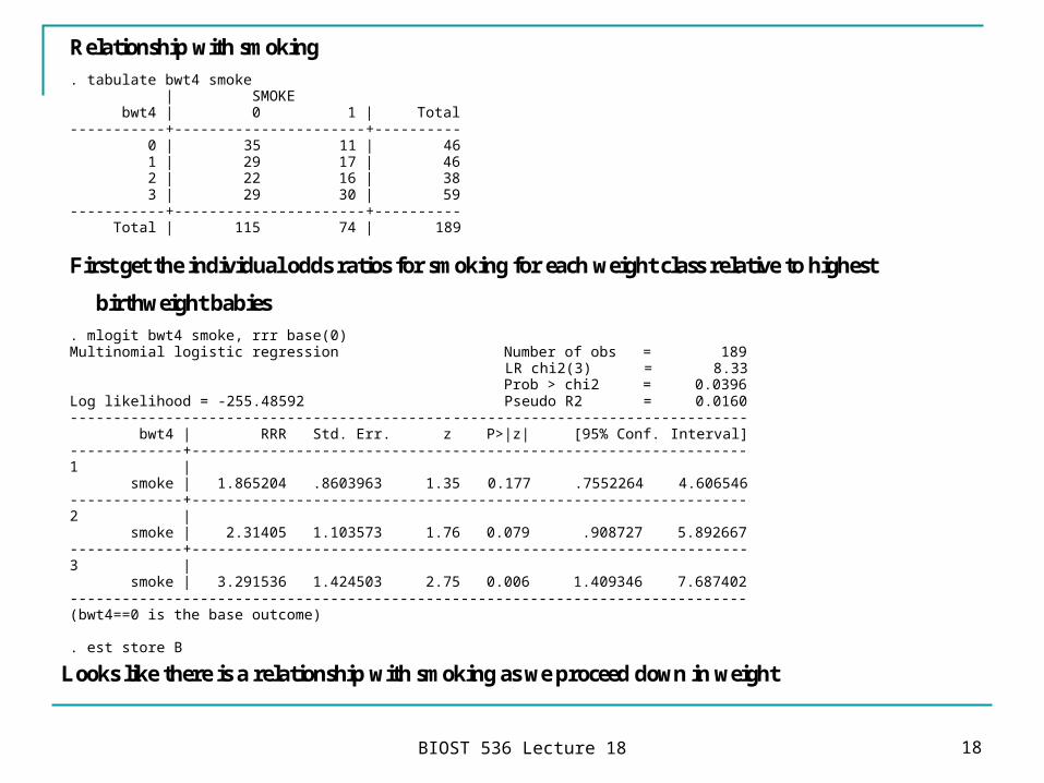
Relationship with smoking . tabulate bwt4 smoke | SMOKE bwt4 | 0 1 | Total -----------+----------------------+---------- 0 | 35 11 | 46 1 | 29 17 | 46 2 | 22 16 | 38 3 | 29 30 | 59 -----------+----------------------+---------- Total | 115 74 | 189
First get the individual odds ratios for smoking for each weight class relative to highest
birthweight babies . mlogit bwt4 smoke, rrr base(0) Multinomial logistic regression Number of obs = 189 LR chi2(3) = 8.33 Prob > chi2 = 0.0396 Log likelihood = -255.48592 Pseudo R2 = 0.0160 ------------------------------------------------------------------------------ bwt4 | RRR Std. Err. z P>|z| [95% Conf. Interval] -------------+---------------------------------------------------------------- 1 | smoke | 1.865204 .8603963 1.35 0.177 .7552264 4.606546 -------------+---------------------------------------------------------------- 2 | smoke | 2.31405 1.103573 1.76 0.079 .908727 5.892667 -------------+---------------------------------------------------------------- 3 | smoke | 3.291536 1.424503 2.75 0.006 1.409346 7.687402 ------------------------------------------------------------------------------ (bwt4==0 is the base outcome) . est store B
Looks like there is a relationship with smoking as we proceed down in weight
BIOST 536 Lecture 18 19
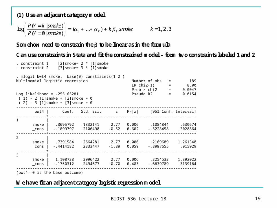
(1) Use an adjacent category model
1 1
( | )log ( ... ) 1, 2, 3
( 0 | ) k
P Y k smokek smoke k
P Y smoke
Somehow need to constrain the to be linear as in the formula
Can use constraints in Stata and fit the constrained model – form two constraints labeled 1 and 2 . constraint 1 [2]smoke= 2 * [1]smoke . constraint 2 [3]smoke= 3 * [1]smoke . mlogit bwt4 smoke, base(0) constraints(1 2 ) Multinomial logistic regression Number of obs = 189 LR chi2(1) = 8.00 Prob > chi2 = 0.0047 Log likelihood = -255.65281 Pseudo R2 = 0.0154 ( 1) - 2 [1]smoke + [2]smoke = 0 ( 2) - 3 [1]smoke + [3]smoke = 0 ------------------------------------------------------------------------------ bwt4 | Coef. Std. Err. z P>|z| [95% Conf. Interval] -------------+---------------------------------------------------------------- 1 | smoke | .3695792 .1332141 2.77 0.006 .1084844 .630674 _cons | -.1099797 .2106498 -0.52 0.602 -.5228458 .3028864 -------------+---------------------------------------------------------------- 2 | smoke | .7391584 .2664281 2.77 0.006 .2169689 1.261348 _cons | -.4414182 .2333447 -1.89 0.059 -.8987655 .015929 -------------+---------------------------------------------------------------- 3 | smoke | 1.108738 .3996422 2.77 0.006 .3254533 1.892022 _cons | -.1750312 .2494677 -0.70 0.483 -.6639789 .3139164 ------------------------------------------------------------------------------ (bwt4==0 is the base outcome)
We have fit an adjacent category logistic regression model
BIOST 536 Lecture 18 20
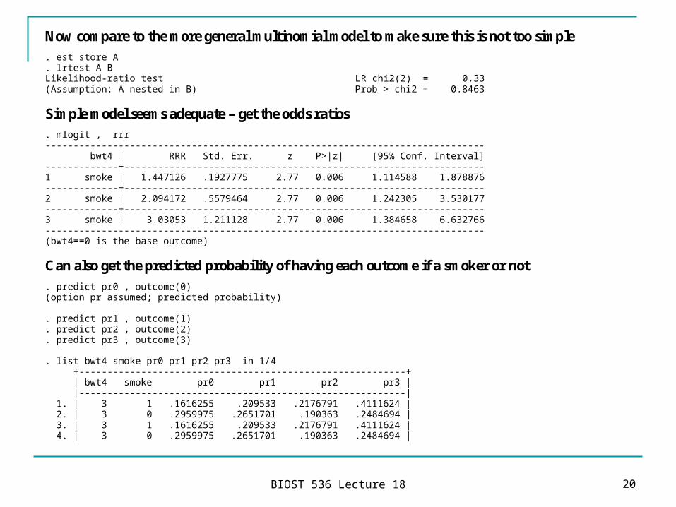
Now compare to the more general multinomial model to make sure this is not too simple . est store A . lrtest A B Likelihood-ratio test LR chi2(2) = 0.33 (Assumption: A nested in B) Prob > chi2 = 0.8463
Simple model seems adequate – get the odds ratios . mlogit , rrr ------------------------------------------------------------------------------ bwt4 | RRR Std. Err. z P>|z| [95% Conf. Interval] -------------+---------------------------------------------------------------- 1 smoke | 1.447126 .1927775 2.77 0.006 1.114588 1.878876 -------------+---------------------------------------------------------------- 2 smoke | 2.094172 .5579464 2.77 0.006 1.242305 3.530177 -------------+---------------------------------------------------------------- 3 smoke | 3.03053 1.211128 2.77 0.006 1.384658 6.632766 ------------------------------------------------------------------------------ (bwt4==0 is the base outcome)
Can also get the predicted probability of having each outcome if a smoker or not . predict pr0 , outcome(0) (option pr assumed; predicted probability) . predict pr1 , outcome(1) . predict pr2 , outcome(2) . predict pr3 , outcome(3) . list bwt4 smoke pr0 pr1 pr2 pr3 in 1/4 +----------------------------------------------------------+ | bwt4 smoke pr0 pr1 pr2 pr3 | |----------------------------------------------------------| 1. | 3 1 .1616255 .209533 .2176791 .4111624 | 2. | 3 0 .2959975 .2651701 .190363 .2484694 | 3. | 3 1 .1616255 .209533 .2176791 .4111624 | 4. | 3 0 .2959975 .2651701 .190363 .2484694 |
BIOST 536 Lecture 18 21
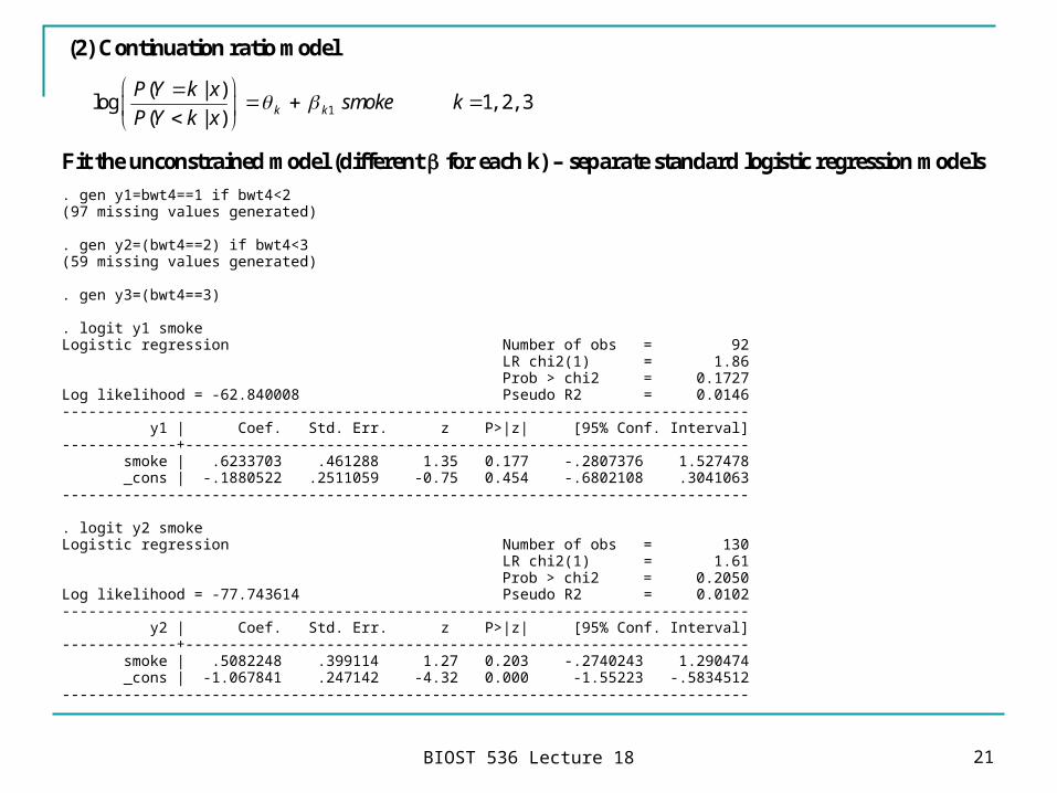
(2) Continuation ratio model
1
( | )log 1, 2, 3
( | ) k k
P Y k xsmoke k
P Y k x
Fit the unconstrained model (different for each k) – separate standard logistic regression models
. gen y1=bwt4==1 if bwt4<2 (97 missing values generated) . gen y2=(bwt4==2) if bwt4<3 (59 missing values generated) . gen y3=(bwt4==3) . logit y1 smoke Logistic regression Number of obs = 92 LR chi2(1) = 1.86 Prob > chi2 = 0.1727 Log likelihood = -62.840008 Pseudo R2 = 0.0146 ------------------------------------------------------------------------------ y1 | Coef. Std. Err. z P>|z| [95% Conf. Interval] -------------+---------------------------------------------------------------- smoke | .6233703 .461288 1.35 0.177 -.2807376 1.527478 _cons | -.1880522 .2511059 -0.75 0.454 -.6802108 .3041063 ------------------------------------------------------------------------------ . logit y2 smoke Logistic regression Number of obs = 130 LR chi2(1) = 1.61 Prob > chi2 = 0.2050 Log likelihood = -77.743614 Pseudo R2 = 0.0102 ------------------------------------------------------------------------------ y2 | Coef. Std. Err. z P>|z| [95% Conf. Interval] -------------+---------------------------------------------------------------- smoke | .5082248 .399114 1.27 0.203 -.2740243 1.290474 _cons | -1.067841 .247142 -4.32 0.000 -1.55223 -.5834512 ------------------------------------------------------------------------------
BIOST 536 Lecture 18 22
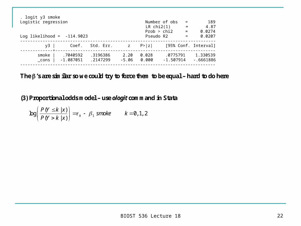
. logit y3 smoke Logistic regression Number of obs = 189 LR chi2(1) = 4.87 Prob > chi2 = 0.0274 Log likelihood = -114.9023 Pseudo R2 = 0.0207 ------------------------------------------------------------------------------ y3 | Coef. Std. Err. z P>|z| [95% Conf. Interval] -------------+---------------------------------------------------------------- smoke | .7040592 .3196386 2.20 0.028 .0775791 1.330539 _cons | -1.087051 .2147299 -5.06 0.000 -1.507914 -.6661886 ------------------------------------------------------------------------------
The ’s are similar so we could try to force them to be equal – hard to do here
(3) Proportional odds model – use ologit command in Stata
1
( | )log 0, 1, 2
( | ) k
P Y k xsmoke k
P Y k x
BIOST 536 Lecture 18 23
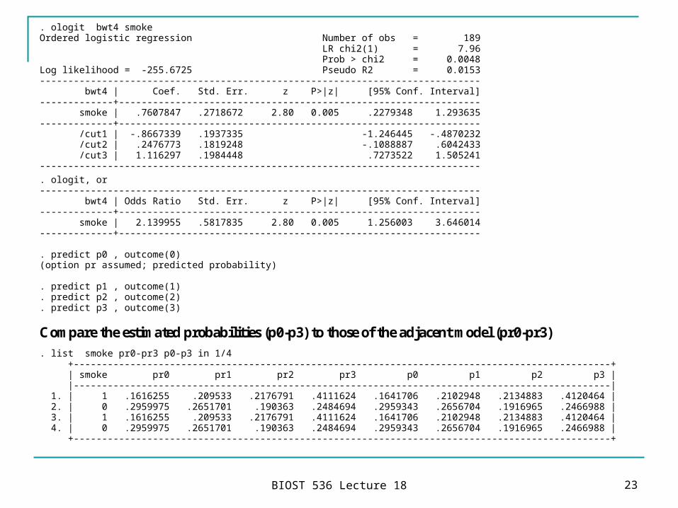
. ologit, or ------------------------------------------------------------------------------ bwt4 | Odds Ratio Std. Err. z P>|z| [95% Conf. Interval] -------------+---------------------------------------------------------------- smoke | 2.139955 .5817835 2.80 0.005 1.256003 3.646014 -------------+---------------------------------------------------------------- . predict p0 , outcome(0) (option pr assumed; predicted probability) . predict p1 , outcome(1) . predict p2 , outcome(2) . predict p3 , outcome(3)
Compare the estimated probabilities (p0-p3) to those of the adjacent model (pr0-pr3) . list smoke pr0-pr3 p0-p3 in 1/4 +-----------------------------------------------------------------------------------------------+ | smoke pr0 pr1 pr2 pr3 p0 p1 p2 p3 | |-----------------------------------------------------------------------------------------------| 1. | 1 .1616255 .209533 .2176791 .4111624 .1641706 .2102948 .2134883 .4120464 | 2. | 0 .2959975 .2651701 .190363 .2484694 .2959343 .2656704 .1916965 .2466988 | 3. | 1 .1616255 .209533 .2176791 .4111624 .1641706 .2102948 .2134883 .4120464 | 4. | 0 .2959975 .2651701 .190363 .2484694 .2959343 .2656704 .1916965 .2466988 | +-----------------------------------------------------------------------------------------------+
. ologit bwt4 smoke Ordered logistic regression Number of obs = 189 LR chi2(1) = 7.96 Prob > chi2 = 0.0048 Log likelihood = -255.6725 Pseudo R2 = 0.0153 ------------------------------------------------------------------------------ bwt4 | Coef. Std. Err. z P>|z| [95% Conf. Interval] -------------+---------------------------------------------------------------- smoke | .7607847 .2718672 2.80 0.005 .2279348 1.293635 -------------+---------------------------------------------------------------- /cut1 | -.8667339 .1937335 -1.246445 -.4870232 /cut2 | .2476773 .1819248 -.1088887 .6042433 /cut3 | 1.116297 .1984448 .7273522 1.505241 ------------------------------------------------------------------------------
BIOST 536 Lecture 18 24
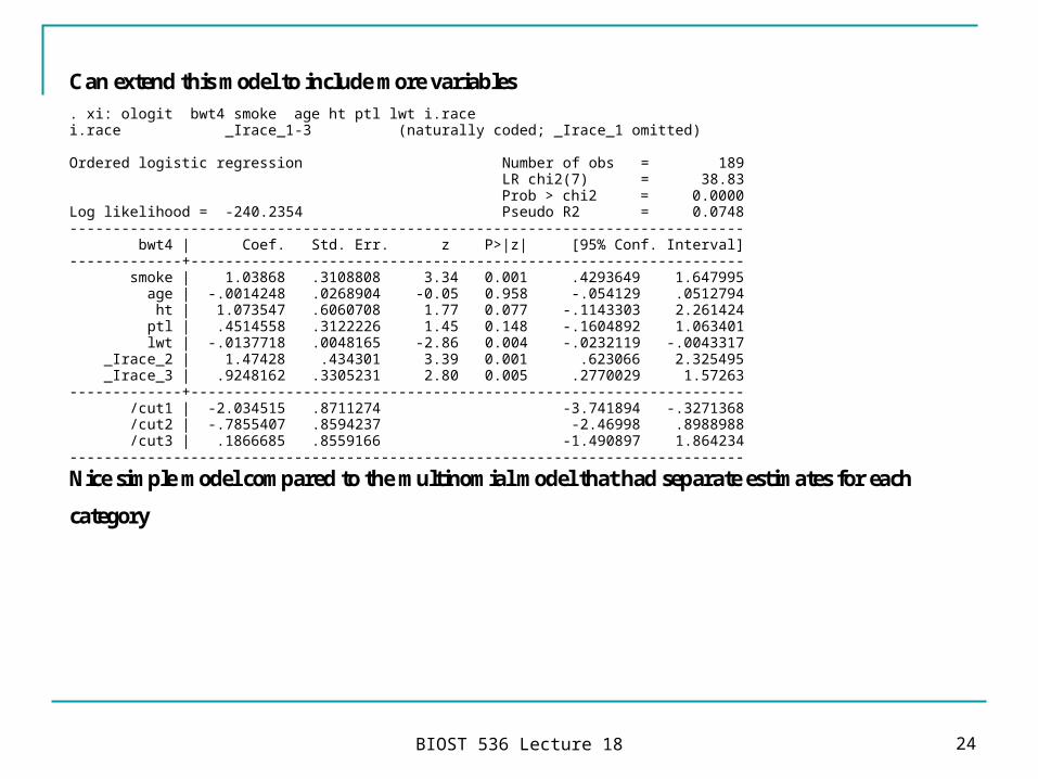
Can extend this model to include more variables . xi: ologit bwt4 smoke age ht ptl lwt i.race i.race _Irace_1-3 (naturally coded; _Irace_1 omitted) Ordered logistic regression Number of obs = 189 LR chi2(7) = 38.83 Prob > chi2 = 0.0000 Log likelihood = -240.2354 Pseudo R2 = 0.0748 ------------------------------------------------------------------------------ bwt4 | Coef. Std. Err. z P>|z| [95% Conf. Interval] -------------+---------------------------------------------------------------- smoke | 1.03868 .3108808 3.34 0.001 .4293649 1.647995 age | -.0014248 .0268904 -0.05 0.958 -.054129 .0512794 ht | 1.073547 .6060708 1.77 0.077 -.1143303 2.261424 ptl | .4514558 .3122226 1.45 0.148 -.1604892 1.063401 lwt | -.0137718 .0048165 -2.86 0.004 -.0232119 -.0043317 _Irace_2 | 1.47428 .434301 3.39 0.001 .623066 2.325495 _Irace_3 | .9248162 .3305231 2.80 0.005 .2770029 1.57263 -------------+---------------------------------------------------------------- /cut1 | -2.034515 .8711274 -3.741894 -.3271368 /cut2 | -.7855407 .8594237 -2.46998 .8988988 /cut3 | .1866685 .8559166 -1.490897 1.864234 ------------------------------------------------------------------------------
Nice simple model compared to the multinomial model that had separate estimates for each
category

BIOST 536 Lecture 18 25
ROC models – actually an ordinal regression model
Usually use a probit link instead of logit for historical reasons but idea is the same
Mammograms are graded on an ordinal scale (y)
Actual result within one year ( 0 = no cancer ; 1 = cancer ) | case y | 0 1 | Total -----------+----------------------+----------
1 | 217,537 199 | 217,736 Normal | 99.91 0.09 | 100.00 -----------+----------------------+----------
2 | 24,536 49 | 24,585 Benign | 99.80 0.20 | 100.00 -----------+----------------------+----------
3 | 4,325 42 | 4,367 Probably benign – short term follow-up | 99.04 0.96 | 100.00 -----------+----------------------+----------
4 | 1,199 10 | 1,209 Probably benign – immediate follow-up | 99.17 0.83 | 100.00 -----------+----------------------+----------
5 | 22,856 769 | 23,625 Indeterminate – additional imaging | 96.74 3.26 | 100.00 -----------+----------------------+----------
6 | 1,156 249 | 1,405 Suspicious | 82.28 17.72 | 100.00 -----------+----------------------+----------
7 | 32 149 | 181 Highly suspicious | 17.68 82.32 | 100.00 -----------+----------------------+---------- Total | 271,641 1,467 | 273,108 | 99.46 0.54 | 100.00
BIOST 536 Lecture 18 26
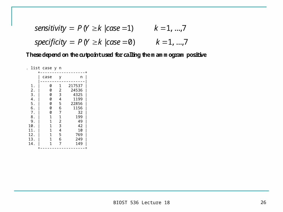
( | 1) 1, ...,7sensitivity P Y k case k
( | 0) 1, ...,7specificity P Y k case k
These depend on the cutpoint used for calling the mammogram positive . list case y n +-------------------+ | case y n | |-------------------| 1. | 0 1 217537 | 2. | 0 2 24536 | 3. | 0 3 4325 | 4. | 0 4 1199 | 5. | 0 5 22856 | 6. | 0 6 1156 | 7. | 0 7 32 | 8. | 1 1 199 | 9. | 1 2 49 | 10. | 1 3 42 | 11. | 1 4 10 | 12. | 1 5 769 | 13. | 1 6 249 | 14. | 1 7 149 | +-------------------+
BIOST 536 Lecture 18 27
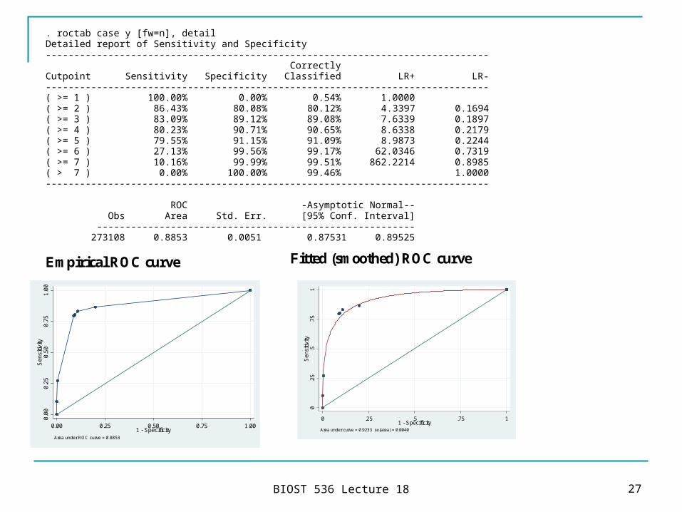
. roctab case y [fw=n], detail Detailed report of Sensitivity and Specificity ------------------------------------------------------------------------------ Correctly Cutpoint Sensitivity Specificity Classified LR+ LR- ------------------------------------------------------------------------------ ( >= 1 ) 100.00% 0.00% 0.54% 1.0000 ( >= 2 ) 86.43% 80.08% 80.12% 4.3397 0.1694 ( >= 3 ) 83.09% 89.12% 89.08% 7.6339 0.1897 ( >= 4 ) 80.23% 90.71% 90.65% 8.6338 0.2179 ( >= 5 ) 79.55% 91.15% 91.09% 8.9873 0.2244 ( >= 6 ) 27.13% 99.56% 99.17% 62.0346 0.7319 ( >= 7 ) 10.16% 99.99% 99.51% 862.2214 0.8985 ( > 7 ) 0.00% 100.00% 99.46% 1.0000 ------------------------------------------------------------------------------ ROC -Asymptotic Normal-- Obs Area Std. Err. [95% Conf. Interval] -------------------------------------------------------- 273108 0.8853 0.0051 0.87531 0.89525
Empirical ROC curve
0.0
00
.25
0.5
00
.75
1.0
0S
ens
itivi
ty
0.00 0.25 0.50 0.75 1.001 - Specificity
Area under ROC curve = 0.8853
Fitted (smoothed) ROC curve
0.2
5.5
.75
1S
ens
itivi
ty
0 .25 .5 .75 11 - Specificity
Area under curve = 0.9233 se(area) = 0.0040
BIOST 536 Lecture 18 28
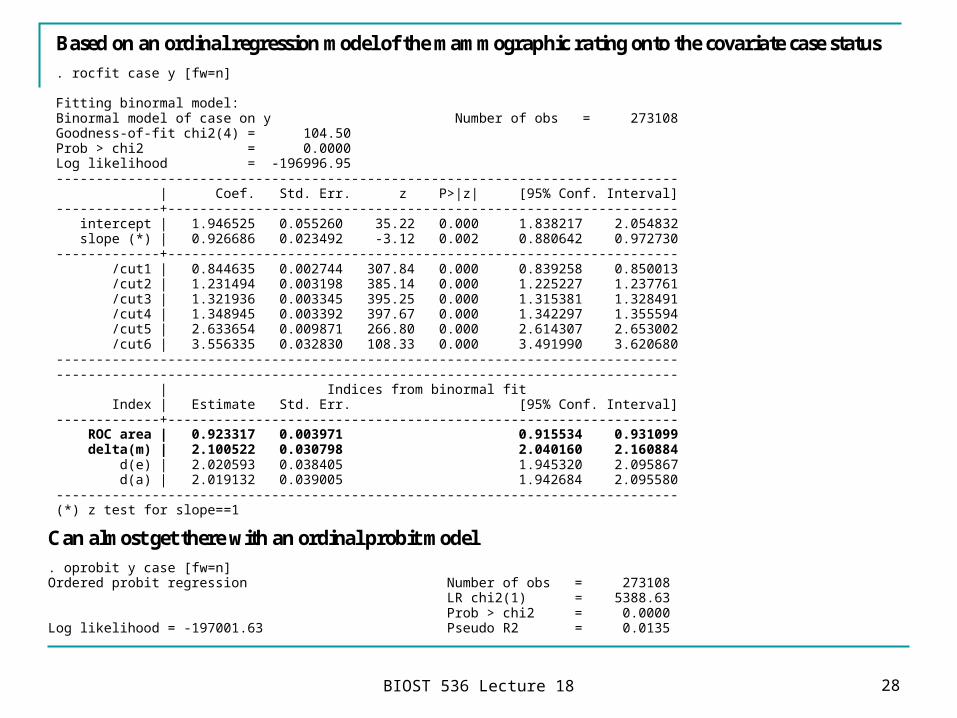
Based on an ordinal regression model of the mammographic rating onto the covariate case status . rocfit case y [fw=n] Fitting binormal model: Binormal model of case on y Number of obs = 273108 Goodness-of-fit chi2(4) = 104.50 Prob > chi2 = 0.0000 Log likelihood = -196996.95 ------------------------------------------------------------------------------ | Coef. Std. Err. z P>|z| [95% Conf. Interval] -------------+---------------------------------------------------------------- intercept | 1.946525 0.055260 35.22 0.000 1.838217 2.054832 slope (*) | 0.926686 0.023492 -3.12 0.002 0.880642 0.972730 -------------+---------------------------------------------------------------- /cut1 | 0.844635 0.002744 307.84 0.000 0.839258 0.850013 /cut2 | 1.231494 0.003198 385.14 0.000 1.225227 1.237761 /cut3 | 1.321936 0.003345 395.25 0.000 1.315381 1.328491 /cut4 | 1.348945 0.003392 397.67 0.000 1.342297 1.355594 /cut5 | 2.633654 0.009871 266.80 0.000 2.614307 2.653002 /cut6 | 3.556335 0.032830 108.33 0.000 3.491990 3.620680 ------------------------------------------------------------------------------ ------------------------------------------------------------------------------ | Indices from binormal fit Index | Estimate Std. Err. [95% Conf. Interval] -------------+---------------------------------------------------------------- ROC area | 0.923317 0.003971 0.915534 0.931099 delta(m) | 2.100522 0.030798 2.040160 2.160884 d(e) | 2.020593 0.038405 1.945320 2.095867 d(a) | 2.019132 0.039005 1.942684 2.095580 ------------------------------------------------------------------------------ (*) z test for slope==1
Can almost get there with an ordinal probit model . oprobit y case [fw=n] Ordered probit regression Number of obs = 273108 LR chi2(1) = 5388.63 Prob > chi2 = 0.0000 Log likelihood = -197001.63 Pseudo R2 = 0.0135
BIOST 536 Lecture 18 29
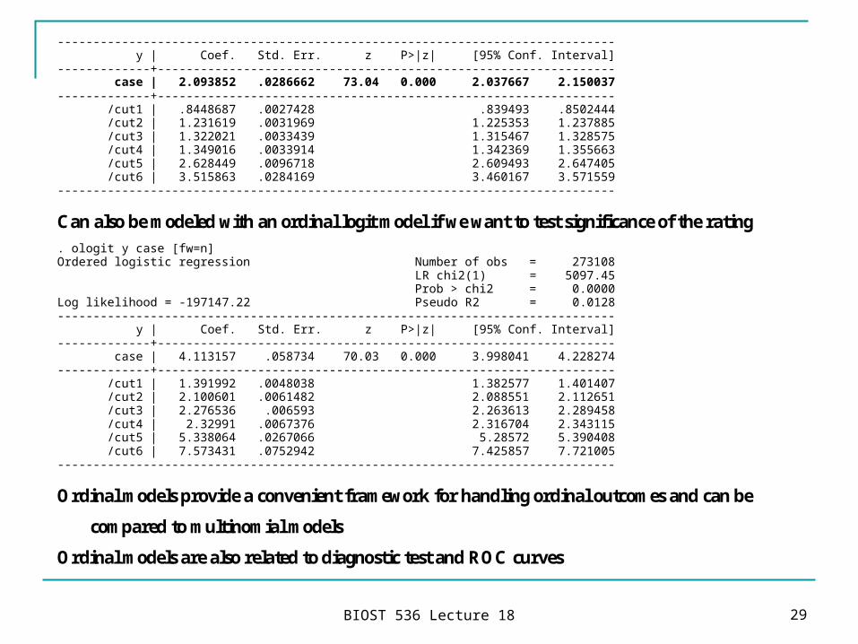
------------------------------------------------------------------------------ y | Coef. Std. Err. z P>|z| [95% Conf. Interval] -------------+---------------------------------------------------------------- case | 2.093852 .0286662 73.04 0.000 2.037667 2.150037 -------------+---------------------------------------------------------------- /cut1 | .8448687 .0027428 .839493 .8502444 /cut2 | 1.231619 .0031969 1.225353 1.237885 /cut3 | 1.322021 .0033439 1.315467 1.328575 /cut4 | 1.349016 .0033914 1.342369 1.355663 /cut5 | 2.628449 .0096718 2.609493 2.647405 /cut6 | 3.515863 .0284169 3.460167 3.571559 ------------------------------------------------------------------------------
Can also be modeled with an ordinal logit model if we want to test significance of the rating . ologit y case [fw=n] Ordered logistic regression Number of obs = 273108 LR chi2(1) = 5097.45 Prob > chi2 = 0.0000 Log likelihood = -197147.22 Pseudo R2 = 0.0128 ------------------------------------------------------------------------------ y | Coef. Std. Err. z P>|z| [95% Conf. Interval] -------------+---------------------------------------------------------------- case | 4.113157 .058734 70.03 0.000 3.998041 4.228274 -------------+---------------------------------------------------------------- /cut1 | 1.391992 .0048038 1.382577 1.401407 /cut2 | 2.100601 .0061482 2.088551 2.112651 /cut3 | 2.276536 .006593 2.263613 2.289458 /cut4 | 2.32991 .0067376 2.316704 2.343115 /cut5 | 5.338064 .0267066 5.28572 5.390408 /cut6 | 7.573431 .0752942 7.425857 7.721005 ------------------------------------------------------------------------------
Ordinal models provide a convenient framework for handling ordinal outcomes and can be
compared to multinomial models
Ordinal models are also related to diagnostic test and ROC curves