binary classification with models and data density distribution by xuan chen
TRANSCRIPT

Binary Classification with Models
and Data Density Distribution
Xuan Chen
E-mail: [email protected]
Supervised by:
Professor Raymond Chi-Wing Wong
E-mail: [email protected]
Abstract. Classification has always been a fundamental topic in data mining.
Traditionally, the study of binary classification has been formulated as a deterministic
problem with 0-1 labels. However, probabilistic information is becoming more popular
nowadays, and it has many practical applications such as pattern recognition as well
as tumour diagnosis. Since probabilistic labels are more informative - they imply
probabilities of the samples belonging to positive cases (i.e., labelled as 1), instead
of plainly stating conclusions, we believe that predictions can be more accurate with
probabilistic labels in training dataset, which is what this project tries to prove.
Keywords: data density distribution, probabilistic labels, error bound, models,
optimization
1. Introduction
1.1. Motivation
Binary classification has its universal application in people’s life: predictions on stock
price, spam email filter, etc. In common cases of binary classification in machine
learning, with a given training dataset T including features X and 0-1 labels Y of
each sample, a model is expected to be created so that when a group of new features
of training dataset are given, its labels can be precisely predicted. However, in real life
situations, probabilistic labels can have a wider range of uses. For example, experts
in many fields often state the probabilities of positive/negative outcomes instead of
giving specific predictions, and a training datasets are often built based on such experts’
justifications. This makes sense, since it would be unfair if experts are required to classify
all the samples with certainty. Hence, in order to obatin meaningful instructions in real
life situations, it would be better if classification with probabilistic information gains
more attention in academic research.
Binary Classification with Models and Data Density Distribution 2
In this paper, in discussion of different data density distribution, we want to find
out whether the accuracy of prediction with the use of probabilistic labels was better
than with traditional results. The conclusion will tell us whether it is worth using
probabilistic labels.
1.2. Binary Classification with Models and Noise Conditions
We study the problem called Binary Classification with Models and Noise Conditions.
Given a training dataset T, with both probabilistic and clear-cut (0-1) labels, we want
to figure out which kind of labels tends make more precise predictions.
Data always follow some sort of distribution. Therefore, data density distribution
such as peak distribution, uniform distribution and convex distribution, and even some
special distribution such as double-arch and double-bowl distribution, were taken into
consideration in this project. Definitions of those data density distribution are specified
in Section 3. We believe that the distributions we mention in this paper are enough to
cover common cases that we are likely to meet in real life.
Moreover, models also have things to do with the accuracy of prediction. Hence,
popular models were involved in our experimental phase. We put those models’
performances with the use of probabilistic labels and clear-cut labels in contrast
respectively. Also, by comparison across different models, we may see which models
relatively do the best work, and which ones improve the most with probabilistic labels
involved. In the end of our experiment, we even tried classification ensemble to improve
when results were not satisfying.
1.3. Contributions
Generally, Gaussian Process Regression works better with probabilistic labels than
with clear-cut labels only when data density follows either bowl distribution, V-shape
distribution, double-arch or double-bowl distribution. With the use of probabilistic
labels and Gaussian Process Regression, as the instances are more found around the
classification boundary, the prediction is less accurate. Also, though Gaussian Process
Regression always performed the best, it is really imperceptible which models improve
the most with the use of probabilistic labels.
Based on theoretical analysis (which is introduced in details in Section 4), with
Gaussian Process Regression and probabilistic labels, prediction error is bounded by
O(n−2+γ4 ) generally[2], where parameter γ determines data density distribution. Under
non-realizable setting, our error bound is always no worse than the best-known error
bound (i.e. O(n−12 ))[5]. Nevertheless, the best-known error bound under realizable
setting is O(n−1)[5], which our result is not necessarily better than.
In experimental phase, we adopted four common models: Gaussian Process
Regression, Radial Basis Function Network, Nearest Neighbour and LibSVM. Generally,
Gaussian Process Regression provided the best prediction. In addition, according to our
experimental result, those models performed much better with probabilistic labels just
Binary Classification with Models and Data Density Distribution 3
when data density followed specific distribution: predictions were more accurate when
instances are farther away from the classification boundary. In those situations when
probabilistic labels had few things to do with prediction, we harnessed classification
ensemble with probability labels and showed that it efficiently improved the accuracy
when data were more found around the classification boundary.
The rest of this paper is organized as follows. In Section 2, we show the source of
common ideas and fundamental knowledge of machine learning and statistical learning
theory, along with the error bounds that were previously obtained. We then give our
problem definition in Section 3. Later on in Section 4, Section 5 and Section 6, we
present our theoretical proofs and experimental results, and we state our observations
based on these. Furthermore, we conclude our work and discuss future works in Section
7. Besides, in the end in Section 8 we talk about challenges and failures that we met
during the process of this project.
2. Related Work
In [5], it has been proven that the error is bounded by O(n−1) for clear-cut training
datasets if data distribution follows realizable assumption (i.e., there exists a classifier
which can perfectly classify any dataset generated from a distribution). In more
general cases that data distribution follows non-realizable assumption, the error of a
classifier is O(n−12 ). On the other hand, with probabilistic labels under Tysbakov Noise
Condition[10], the error produced by Gaussian Process Regression goes down to O(n2+γ4 )
(where γ ≥ 0)[2]. Our discussion of different data density distribution is a derivative
of such a result. Our result is never worse than the error bound offered by [5] under
non-realizable setting in any distribution. However, under realizable setting, with data
density following uniform or peak distribution, our error bound is unfortunately worse
than the one given by [5]. Analysis is stated in Section 4.
Common ideas in statistical learning theory were mostly introduced in [6], and basic
concepts were introduced in [8].
3. Problem Definition
3.1. Training datasets
Consider a binary classification with two classes, 0 and 1. In traditional setting, we are
given a training dataset T which contains n instances I1, I2, ..., In. Each instance Iiis associated with a feature vector xi and a target attribute yi where i ∈ N. Let X be
the set of all possible feature vectors. Note that there are two possible values of target
attribute yi, namely 0 and 1. A classifier h is defined to be a hypothesis or a function
which takes feature vector xi as an input and its output yi is either 0 or 1.
Now let’s turn to classification with probabilistic information. Similar to traditional
setting, T contains n instances, namely I1, I2, ..., In. We assume that the data samples
in the dataset are independent and identically distributed (i.i.d).Each instance Ii is
Binary Classification with Models and Data Density Distribution 4
associated with a feature vector xi and a fractional score fi (rather than a target
attribute yi) where i ∈ N. We assume that all instances are generated according to
a joint distribution of two random variables, X and Y , denoted by Pr(X,Y ). Given a
feature vector x, we define η(x) to be the conditional probability Pr(Y = 1|X = x),
the probability that an instance with its feature xi has its target attribute equal to 1.
η(x) is the estimated probability, i.e., η(x) can be considered as the computed
version of η(x) provided by models.
Since fractional score fi is obtained by labelers and some statistical information, it
can be regarded as an observed version of η(xi). To be more specific, fi is the value η(xi)
added by Gaussian white noise. The Gaussian white noise is represented in the form
of Gaussian distribution N (0, σ2) where σ is a standard deviation of this distribution.
With this noise condition, each fractional score fi follows the distribution of N (0, σ2).
If fi is smaller than 0, then it can be assigned to class 0. Likewise, if fi is larger than
1, then it can be assigned to class 1.
3.2. Measurement of error
It is assumed that the excess error of a given classifier corresponds to the difference
between the expected error generated by this classifier and the expected error generated
by the best classifier.
Given a classifier h = Iη(x)≥0.5, the expected error of h, denoted by err(h), is defined
to be Pr(x,y)∼Pr(X,Y )(y 6= h(x)). The Bayes classifier, denoted by h∗, is defined to be
the classifier which gives the minimum expected error. Note that h∗ = Iη(x)≥0.5. Given
a classifier h, its excess error is defined as the difference between its expected error
and the expected error of h∗, i.e., the excess error of h, denoted by E(h), is equal to
err(h) − err(h∗). Note that E(h) must be greater than 0. Apparently, the hypothesis
is more accurate when E(h) is approaching 0.
In a word, when η(x) is very similar to η(x), our classifiers perform as good as
optimal achievable classifier(i.e. Bayes Classifier).
3.3. Data density distribution
First of all, we state the definition of Tysbakov Noise Condition.
Definition 3.1. (Tysbakov Noise Condition) Given two noise parameters c > 0 and
γ ≥ 0, ∀t ∈ (0, 0.5),
Pr(E[|η(x)− 1/2|] < t) ≤ c · tγ.
Define f(t) = ctγ. Then g(t) = f ′(t) = cγ · tγ−1 = cγ · ta reflects the distribution
of data density. The distributions are symmetrical about η(x) = 12. Let’s discuss the
cases of different values of γ. Note that in discussion we take ”=” of the formula. But
actually, since the definition is an in-equation, distribution that under the curves we
draw in Figure 1-5 (i.e., smaller than c · tγ) can be attributed to its corresponding case.
Binary Classification with Models and Data Density Distribution 5
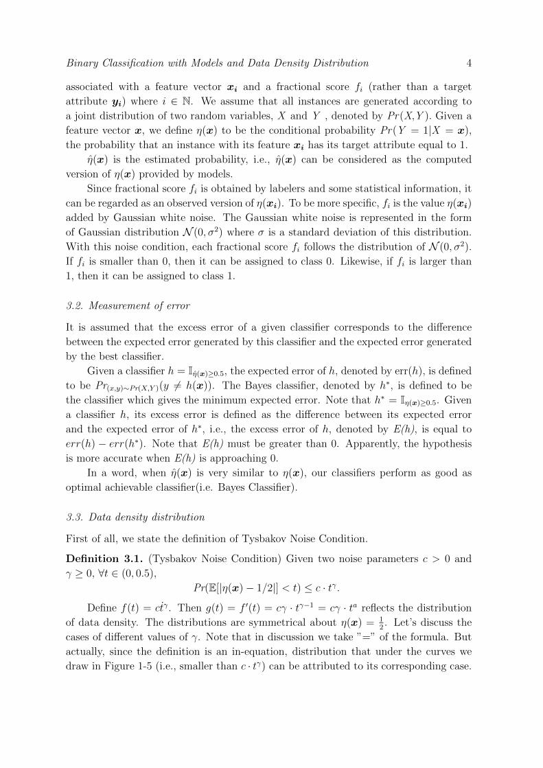
3.3.1. Convex Distribution Cases of convex distribution is shown in Figure 1.
1© Bowl-shape Distribution: When
γ > 2, g′(t) starts from 0 and increases
as t increases. Therefore, data density in
terms of η(x) looks like a bowl.
2© V-shape Distribution: When γ =
2, a = 1 and g(t) is a linear function.
So data density in terms of η(x) is a
symmetrical V-shape and the lowest point
occurs at η(x) = 12.
3© Cusp Distribution: When 1 < γ <
2, 0 < a < 1 and g′(t) decreases but
always larger than 0 as t increases. As a result, data density in terms of η(x) is a
cusp.
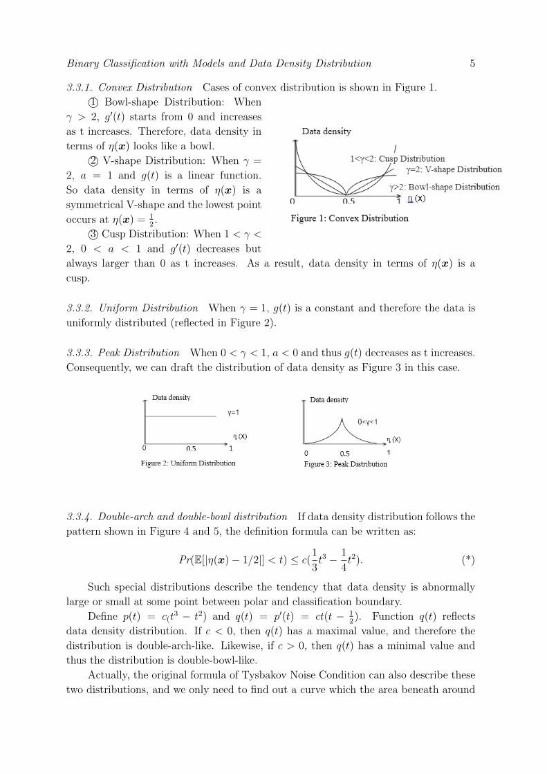
3.3.2. Uniform Distribution When γ = 1, g(t) is a constant and therefore the data is
uniformly distributed (reflected in Figure 2).
3.3.3. Peak Distribution When 0 < γ < 1, a < 0 and thus g(t) decreases as t increases.
Consequently, we can draft the distribution of data density as Figure 3 in this case.
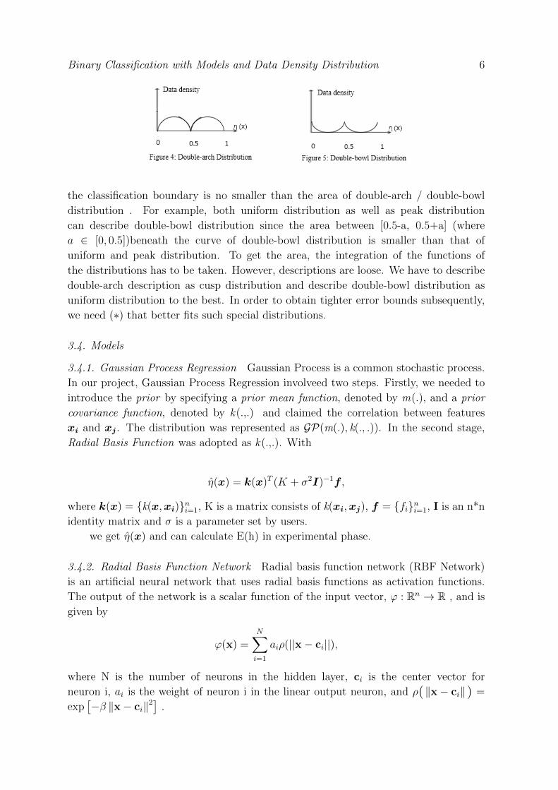
3.3.4. Double-arch and double-bowl distribution If data density distribution follows the
pattern shown in Figure 4 and 5, the definition formula can be written as:
Pr(E[|η(x)− 1/2|] < t) ≤ c(1
3t3 − 1
4t2). (*)
Such special distributions describe the tendency that data density is abnormally
large or small at some point between polar and classification boundary.
Define p(t) = c(t3 − t2) and q(t) = p′(t) = ct(t − 1
2). Function q(t) reflects
data density distribution. If c < 0, then q(t) has a maximal value, and therefore the
distribution is double-arch-like. Likewise, if c > 0, then q(t) has a minimal value and
thus the distribution is double-bowl-like.
Actually, the original formula of Tysbakov Noise Condition can also describe these
two distributions, and we only need to find out a curve which the area beneath around
Binary Classification with Models and Data Density Distribution 6
the classification boundary is no smaller than the area of double-arch / double-bowl
distribution . For example, both uniform distribution as well as peak distribution
can describe double-bowl distribution since the area between [0.5-a, 0.5+a] (where
a ∈ [0, 0.5])beneath the curve of double-bowl distribution is smaller than that of
uniform and peak distribution. To get the area, the integration of the functions of
the distributions has to be taken. However, descriptions are loose. We have to describe
double-arch description as cusp distribution and describe double-bowl distribution as
uniform distribution to the best. In order to obtain tighter error bounds subsequently,
we need (∗) that better fits such special distributions.
3.4. Models
3.4.1. Gaussian Process Regression Gaussian Process is a common stochastic process.
In our project, Gaussian Process Regression involveed two steps. Firstly, we needed to
introduce the prior by specifying a prior mean function, denoted by m(.), and a prior
covariance function, denoted by k(.,.) and claimed the correlation between features
xi and xj . The distribution was represented as GP(m(.), k(., .)). In the second stage,
Radial Basis Function was adopted as k(.,.). With
η(x) = k(x)T (K + σ2I)−1f ,
where k(x) = {k(x,xi)}ni=1, K is a matrix consists of k(xi,xj), f = {fi}ni=1, I is an n*n
identity matrix and σ is a parameter set by users.
we get η(x) and can calculate E(h) in experimental phase.
3.4.2. Radial Basis Function Network Radial basis function network (RBF Network)
is an artificial neural network that uses radial basis functions as activation functions.
The output of the network is a scalar function of the input vector, ϕ : Rn → R , and is
given by
ϕ(x) =N∑i=1
aiρ(||x− ci||),
where N is the number of neurons in the hidden layer, ci is the center vector for
neuron i, ai is the weight of neuron i in the linear output neuron, and ρ(‖x− ci‖
)=
exp[−β ‖x− ci‖2
].

Binary Classification with Models and Data Density Distribution 7
3.4.3. Nearest Neighbour Nearest Neighbors algorithm is a non-parametric method
used for classification and regression. An object is classified by a majority vote of its
neighbors, with the object being assigned to the class most common among its k nearest
instances. For implementation of this algorithm, the nearer neighbors contribute more
to the justification of unknown instances. For example, a common weighting scheme
gives each neighbor a weight of 1/d, where d is the distance to the neighbor.
3.4.4. Support Vector Machine Support vector machines (SVMs) are supervised
learning models with associated learning algorithms that analyze data and recognize
patterns. Since SVM is a well-known and popular technique that has many variants, we
do not include detailed introductions in this paper. Intuitions of SVMs can be found in
[7].
In this project, we used a SVM algorithm called LibSVM [9] brought out by Chih-
Chung Chang and Chih-Jen Lin.
3.5. Problem
In this project, we study whether in every data density distribution can the models
perform better with probabilistic labels than with clear-cut labels. We give proofs when
Gaussian Process Regression is harnessed as our model. For other popular models,
though we do not give theoretical analysis, we still adopted them to our experiments
and have had our observations.
4. Theoretical Analysis
The following analysis is for Gaussian Process Regression.
We start up with the proof in [1].
E(h) = Pr(Y 6= h(x))− Pr(Y 6= h∗(x))
= E[|2η(x)− 1| · |h(x)− h∗(x)|]≤ 2E[|η(x)− η(x)| · Pr(h(x) 6= h∗(x))]
≤ 2√E[(η(x)− η(x))2] ·
√Pr(h(x) 6= h∗(x))
(1)
Please note that when h(x) 6= h∗(x), we have |η(x)− 12| ≤ |η(x)− η(x)|. Because
if η(x) ≤ 12, η(x) > 1
2and thus η(x) and η(x) stand on two sides of 1
2. If η(x) > 1
2, the
proof and conclusion are similar.
With probability of at least 1− δ, by proving
E[(η(x)− f)2] ≤ ∆ (2)
where
∆ ∈ O(n−1), (3)
Binary Classification with Models and Data Density Distribution 8
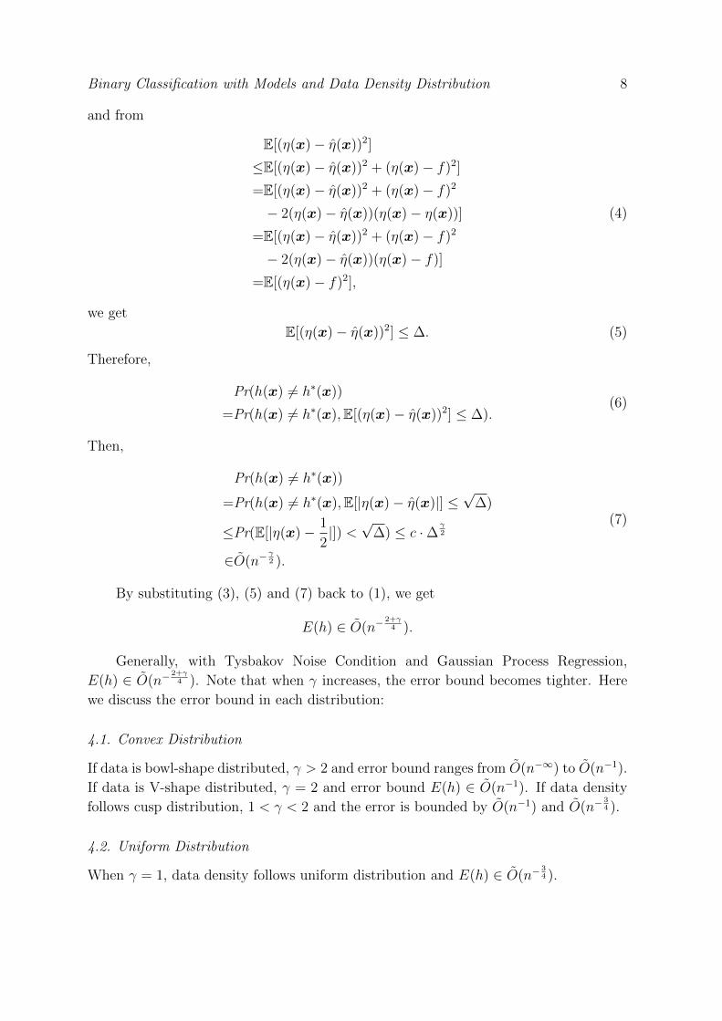
and from
E[(η(x)− η(x))2]
≤E[(η(x)− η(x))2 + (η(x)− f)2]
=E[(η(x)− η(x))2 + (η(x)− f)2
− 2(η(x)− η(x))(η(x)− η(x))]
=E[(η(x)− η(x))2 + (η(x)− f)2
− 2(η(x)− η(x))(η(x)− f)]
=E[(η(x)− f)2],
(4)
we get
E[(η(x)− η(x))2] ≤ ∆. (5)
Therefore,
Pr(h(x) 6= h∗(x))
=Pr(h(x) 6= h∗(x),E[(η(x)− η(x))2] ≤ ∆).(6)
Then,
Pr(h(x) 6= h∗(x))
=Pr(h(x) 6= h∗(x),E[|η(x)− η(x)|] ≤√
∆)
≤Pr(E[|η(x)− 1
2|]) <
√∆) ≤ c ·∆
γ2
∈O(n−γ2 ).
(7)
By substituting (3), (5) and (7) back to (1), we get
E(h) ∈ O(n−2+γ4 ).
Generally, with Tysbakov Noise Condition and Gaussian Process Regression,
E(h) ∈ O(n−2+γ4 ). Note that when γ increases, the error bound becomes tighter. Here
we discuss the error bound in each distribution:
4.1. Convex Distribution
If data is bowl-shape distributed, γ > 2 and error bound ranges from O(n−∞) to O(n−1).
If data is V-shape distributed, γ = 2 and error bound E(h) ∈ O(n−1). If data density
follows cusp distribution, 1 < γ < 2 and the error is bounded by O(n−1) and O(n−34 ).
4.2. Uniform Distribution
When γ = 1, data density follows uniform distribution and E(h) ∈ O(n−34 ).
Binary Classification with Models and Data Density Distribution 9
4.3. Peak Distribution
In this situation 0 ≤ γ < 1. Hence the error is better than O(n−12 ) but worse than
O(n−34 ).
4.4. Double-arch and double-bowl distribution
As defined in Section 3,
Pr(E[|η(x)− 1/2|] <√
∆) ≤ c(1
3∆
32 − 1
4∆1) ∈ O(n−1).
Hence,
E(h) ≤ 2√E[(η(x)− η(x))2] ·
√Pr(h(x) 6= h∗(x))
∈O(n−12 ) · O(n−
12 ) = O(n−1)
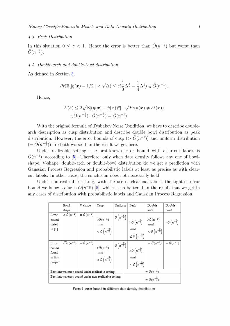
With the original formula of Tysbakov Noise Condition, we have to describe double-
arch description as cusp distribution and describe double bowl distribution as peak
distribution. However, the error bounds of cusp (> O(n−1)) and uniform distribution
(= O(n−34 )) are both worse than the result we get here.
Under realizable setting, the best-known error bound with clear-cut labels is
O(n−1), according to [5]. Therefore, only when data density follows any one of bowl-
shape, V-shape, double-arch or double-bowl distribution do we get a prediction with
Gaussian Process Regression and probabilistic labels at least as precise as with clear-
cut labels. In other cases, the conclusion does not necessarily hold.
Under non-realizable setting, with the use of clear-cut labels, the tightest error
bound we know so far is O(n−12 ) [5], which is no better than the result that we get in
any cases of distribution with probabilistic labels and Gaussian Process Regression.
Binary Classification with Models and Data Density Distribution 10
5. Experiment
We conducted experiments via Weka (Waikato Environment for Knowledge Analysis)
3.6, a popular suite of machine learning software written in Java, on a workstation with
2.10 GHz CPU and 2.0 GB RAM.
During experiments, we selected real datasets Model Years, Student Performance
and Wine Quality originally for regression from UCI repositary[12], and Cadata and
Body Fat from [13]. The normalized value of the target attribute of each instance
ranging from 0 to 1 was seen as the probability that the instance belongs to class 1.
The first dataset is Model Years, whose data roughly follows bowl-shape distribution
(data become sparser while approaching classification boundary 0.5). The second one
is Cadata, with uniformly distributed data in it. Data in Student Performance follows
peak distribution. We also tested dataset named Wine Quality and Body Fat, whose
data can be observed to be double-arch distributed.
As stated in Section 3, we are only given an observed version of the probabilistic
dataset, says Tf . Thus, we generate Tf by adding a noise value randomly picked from
N (0, σ) to each probability. Each added value corresponds to a fractional score in Tf .
Note that if the added value is greater than 1, we reset it to 1. If it is smaller than 0,
we attribute it to 0. In all experiments, we set σ = 0.01 as default.
We implemented our proposed classifier based on Gaussian Process Regression.
Though in theoretical analysis, we only study the error bound with the use of (1)
Gaussian Process Regression, here we also considered three other common comparative
classifiers in our experiment: (1) Radial Basis Function Network (RBF Network),
(2) Nearest Neighbour and (3) LibSVM. We ran all those four classifiers with both
probabilistic labels and clear-cut labels. Those classifications are introduced in Section
3.4. Note that (4) LibSVM is only available for clear-cut labels. Hence we merely ran
it on datasets with 0-1 labels in our experiments. We gave trials with different models
to see how models performed when probabilistic labels were adopted in prediction.
We performed a 10-fold cross validation for these experiments. The training
datasets was randomly divided into 10 pieces, each of which was regarded as testing
dataset in one of the ten folds, while the rest worked for training. We evaluate a
classifier in terms of its average accuracy on the held-out test set.
5.1. Model Years
Here is the distribution of data in Model Years. Left is the distribution of clear-cut
labels, with the distribution of probabilistic labels on the right. Apparently, data roughly
followed bowl-shape distribution.

Binary Classification with Models and Data Density Distribution 11
The chart in below presents the performance of each model with both clear-cut
labels as well as probabilistic labels.
From the chart we can find out that, with probabilistic labels, the prediction was
more accurate not only when the model was Gaussian Process Regression, as we prove in
Section 4, but when the model was RBF Network or Nearest Neighbour. Additionally,
it is interesting to notice that Nearest Neighbour classifier with probabilistic labels also
had satisfying performance, just a little bit behind Gaussian Process Regression. The
result supported our analysis that when data is bowl-shape distributed, prediction with
probabilistic labels is more accurate than with clear-cut labels.
5.2. Cadata
Here is the distribution of data in Cadata. Data followed uniform distribution.
The chart in below presents the performance of each model with both clear-cut
labels as well as probabilistic labels.
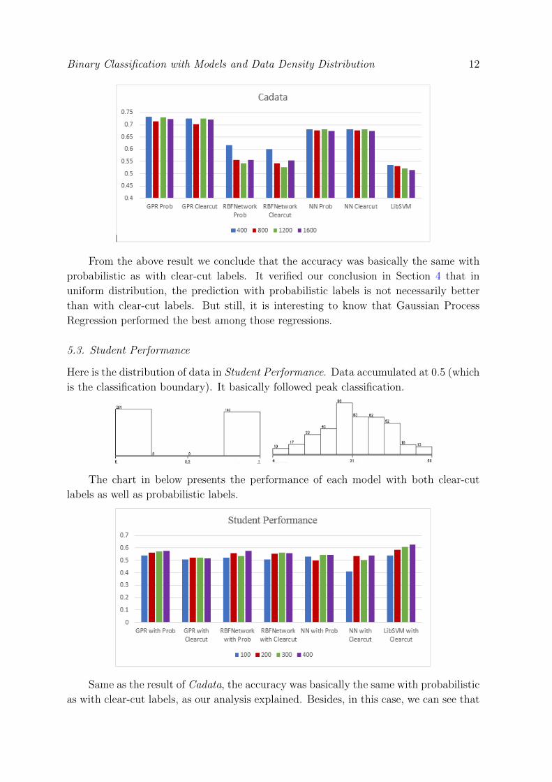
Binary Classification with Models and Data Density Distribution 12
From the above result we conclude that the accuracy was basically the same with
probabilistic as with clear-cut labels. It verified our conclusion in Section 4 that in
uniform distribution, the prediction with probabilistic labels is not necessarily better
than with clear-cut labels. But still, it is interesting to know that Gaussian Process
Regression performed the best among those regressions.
5.3. Student Performance
Here is the distribution of data in Student Performance. Data accumulated at 0.5 (which
is the classification boundary). It basically followed peak classification.
The chart in below presents the performance of each model with both clear-cut
labels as well as probabilistic labels.
Same as the result of Cadata, the accuracy was basically the same with probabilistic
as with clear-cut labels, as our analysis explained. Besides, in this case, we can see that

Binary Classification with Models and Data Density Distribution 13
prediction with Gaussian Process Regression was not outstanding anymore. All models
involved gave around the same accuracy.
5.4. Wine Quality
Here is the distribution of data in Wine Quality. Double-arch distribution is able to
best describe the distribution.
The conclusion from this result is similar to what we’ve got from Model Years : the
improvement on prediction accuracy was obvious when probabilistic labels was put in
use. In addition, in this case Gaussian Process Regression still had the best performance.
5.5. Body Fat
Here is the distribution of data in Body fat. Double-arch distribution is able to best
describe the distribution.
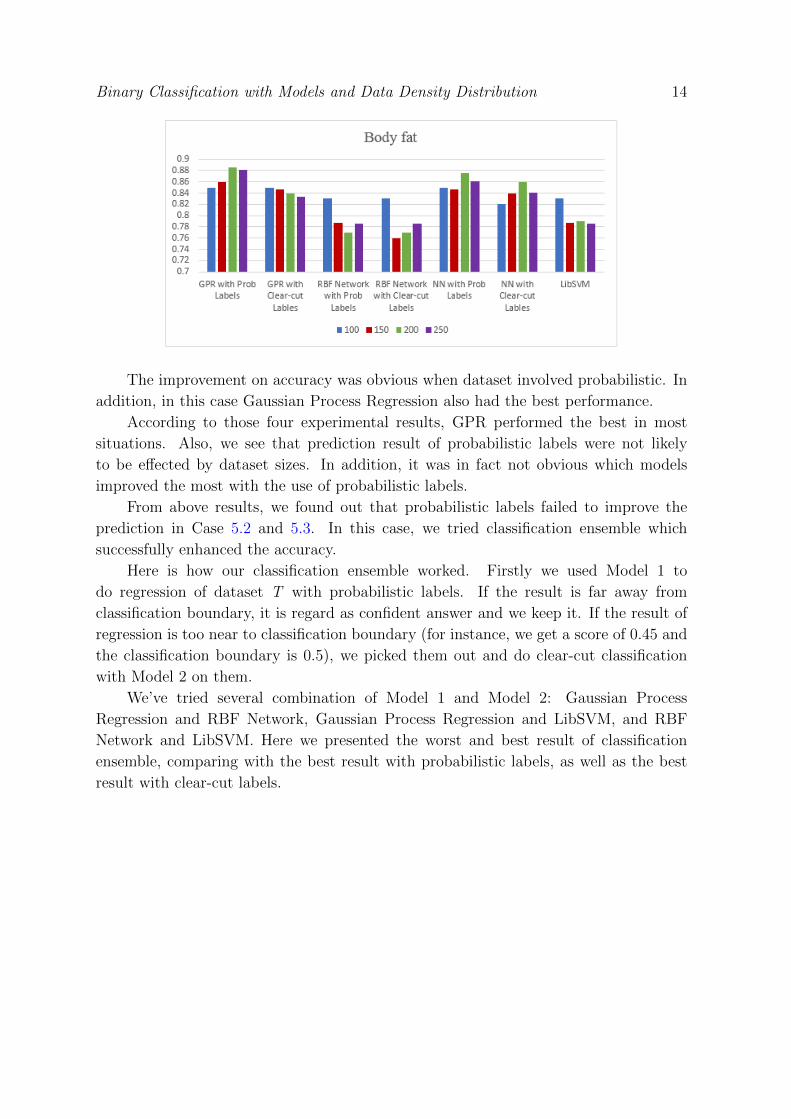
Binary Classification with Models and Data Density Distribution 14
The improvement on accuracy was obvious when dataset involved probabilistic. In
addition, in this case Gaussian Process Regression also had the best performance.
According to those four experimental results, GPR performed the best in most
situations. Also, we see that prediction result of probabilistic labels were not likely
to be effected by dataset sizes. In addition, it was in fact not obvious which models
improved the most with the use of probabilistic labels.
From above results, we found out that probabilistic labels failed to improve the
prediction in Case 5.2 and 5.3. In this case, we tried classification ensemble which
successfully enhanced the accuracy.
Here is how our classification ensemble worked. Firstly we used Model 1 to
do regression of dataset T with probabilistic labels. If the result is far away from
classification boundary, it is regard as confident answer and we keep it. If the result of
regression is too near to classification boundary (for instance, we get a score of 0.45 and
the classification boundary is 0.5), we picked them out and do clear-cut classification
with Model 2 on them.
We’ve tried several combination of Model 1 and Model 2: Gaussian Process
Regression and RBF Network, Gaussian Process Regression and LibSVM, and RBF
Network and LibSVM. Here we presented the worst and best result of classification
ensemble, comparing with the best result with probabilistic labels, as well as the best
result with clear-cut labels.

Binary Classification with Models and Data Density Distribution 15
Basically, predictions given by classification ensemble were always no worse than
our former results. Particularly, there always existed some combination of classification
ensemble whose prediction was much better.
6. Discussion
Intuitively, with probabilistic labels models are able to predict much more precise
estimated target attribute. However, such an advantage does not show when instances
are located around the classification boundary. For example, there is an instance labelled
as 0.49999 and is attributed to class 0. Though with probabilistic labels we are able to
predict estimated probability as 0.50001, which is pretty close to the true value whereas
it should be attributed to class 1 by models and is thus wrong. In a word, when more
data are founded around the classification boundary, the prediction is much less accurate
with probabilistic labels. This perfectly explain why the prediction error of Gaussian
Process Regression with probabilistic labels is no worse than the best-known error bound
under any setting with clear-cut labels only when γ is large enough.
7. Conclusion
In this paper, we study the worth of probabilistic labels, which depends on the data
density distribution. Generally, when data are more observed around the classification
boundary, predictions with probabilistic labels are not necessarily better than with clear-
cut labels. However, we can try classification ensembles in those cases, and the accuracy
can be better than the result when we use probabilistic or clear-cut labels solely.
Besides, from experimental result we can conclude that GPR performed the best
in most situations, whereas it was hard to define which models were improved the most
when probabilistic labels were involved.
Acknowledgements:The author would like to thank the supervisor of this project,
Professor Raymond Chi-Wing Wong, for always arranging meetings during which he
helped the the author to look at this final year thesis from different points of view, offered
Binary Classification with Models and Data Density Distribution 16
useful materials for learning, and gave good advice when the author had difficulties in
proofs.
The author would also like to thank Mr. Peng Peng, a PhD candidate at HKUST
under the supervision of Professor Wong, for always arranging advisory discussions
whenever the author asked for help. He helped the author understand machine learning
and clarify proofs and ideas in [2] at the beginning, and he always readily provided helps
when the author got stuck in thinking of ideas in his final year thesis.
Besides, the author would like to thank Mr. Ted Spaeth, who is the Final Year
Thesis Tutor. He paid a lot of time reviewing and rectifying the reports of this project.
He has also been giving much advice for improving the writing and presentation.
8. Challenges and Future Work
We met some challenges during the process of this project.
We wanted to prove whether some other algorithms gives out better performance
with the use of probabilistic labels. We tried to follow the ideas presented in [2],
whereas Gaussian Process Regression has its speciality:∑n
i=1(η(xi)−fi)2 ∈ O(1), where
η(xi) is estimated probability got from models and fi is observed version of conditional
probability η(xi). In this case the deviations were no longe ravailable. We then tried
to introduced Hausser’s Theorem, VC Dimension and VC entropy, along with Covering
Numbers, whereas none of them provides promising insights and description of a smaller
error bounds.
Therefore, there are interesting future works and room for improvement. By
considering algorithms, we may see whether our conclusion is also suitable for other
classifiers.
References
[1] P. Peng and R. Wong, Selective Sampling on Probabilistic Data, Proc. 2014 Int’l Data Mining
(SDM 14), 28-36.
[2] P. Peng, R. Wong, P. Yu, Learning on Probabilistic Labels, Proc. 2014 Int’l Data Mining (SDM
14), 307-315.
[3] Q. Nguyen, H. Valizadegan, M. Hauskrecht, Learning Classification with Auxiliary Probabilistic
Information, Proc. 2011 IEEE int’l Conf. on Data Mining (ICDM 2011), 477-486.
[4] M. Ebden, Gaussian Process for Regression: A Quick Introduction,
http://www.robots.ox.ac.uk/ mebden/reports/GPtutorial.pdf, 1-5.
[5] M. Anthony, P. L. Bartlett, Neural Network Learning: Theoretical Foundations, March 1994,
Cambridge University Press 1999, 278.
[6] Q. Bousquet, S. Boucheron,G. Lugosi, Introduction to Statistical Learning Theory,
www.kyb.mpg.de/publications/pdfs/pdf2819.pdf, 179-213.
[7] A. Ng, Introduction of Support Vector Machine, http://cs229.stanford.edu/notes/cs229-notes3.pdf.
[8] A. Ng, CS229: Machine Learning, http://Coursera.org, 2014.
[9] C. Chang, C. Lin, LibSVM, http://www.csie.ntu.edu.tw/ cjlin/libsvm/
[10] A. Tysbakov, Optimal aggregation of classifiers in statistical learning, The Annals of Statistics
2004, 135-166.

Binary Classification with Models and Data Density Distribution 17
[11] P. Massart, E. Nedelec, Risk Bounds for Statistical Learning, The Annals of Statistics 2006, 2326-
2366.
[12] A. Frank,A. Asuncion, UCI machine learning repositary, https://archive.ics.uci.edu/ml/datasets.html
[13] Department of Statistics at Carnegie Mellon University, StatLib, http://lib.stat.cmu.edu/