bidding tendencies in the gulf of mexico · bidding tendencies in the gulf of mexico ... bids along...

Running Header: Final Project

The Pennsylvania State University

Department of Geography

Bidding Tendencies in the Gulf of Mexico

by

Fabian Guarin Angarita

Master of GIS

2016


Abstract

The US Federal government through the Bureau of Ocean Energy Management (BOEM) leases acreage

in the offshore Gulf of Mexico (GOM). The BOEM leasing program includes 93.75 million acres in one of

the most productive petroleum basins in the world. This project explores the geographic distribution of

bids in the GOM by analyzing bid amount and locations. The study includes the identification of hot

spots where bids are more frequent or higher, and indicates industry areas of interest.

Introduction

In today’s dynamic world, millions of people are generating a demand for energy, specifically oil. We

participate in creating this demand by continuously going to the gas station and pump some refined oil

into our cars. This gasoline is the result of an exploration process that started many years before. In this

project I focus on the initial steps were lands are leased to exploration companies that search for this

energy resource.

The goal of this project is to identify trends between lease bids and their location. I will be exploring the

patterns in bid locations and how their location and price tend to cluster.

Background of the Topic:

Every year the Federal government lease out 3x3 mile blocks of offshore federal land in the Gulf of

Mexico. According to the BOEM, in the last lease sale in 2015, 21 million acres were available in the

western Gulf of Mexico lease sale (BOEM 2013). The bids have a wide price range, and in some cases for

a 10 year lease the bids go up into the 100 million dollars.

The Bureau of Ocean Energy Management, Regulation, and Enforcement (BOEMRE) dictates the rules

and dates when lease sales take place. It also regulates the standards and conditions for these leases

(Nomack 2010).

Usually a block is leased for 5 to 10 years. Small blocks close to the coast are leased for 5 years, and

blocks in water deeper than 1000 feet are leased for 10 years (Crawford et al., 2008). The bids for the

lots are secret until the date of the lease sale. The day of the lease sale, the bids are made public and are

read aloud at a public meeting.

Research Question:

This project intends to find geographical distribution patterns of the lease sale bids. In addition, I seek to

determine if bids have cluster patterns and, if so, determine where similar bids group forming hot and

cold spots. I hope to find out if there is a pattern in the monetary value of bids by creating point

samples that represent each GOM lease block, and assigning the dollar value to each point.

To limit the scope of this project I only use lease data that are current. No historic dollar offers on the

same lease sale or on different leases will be analyzed.


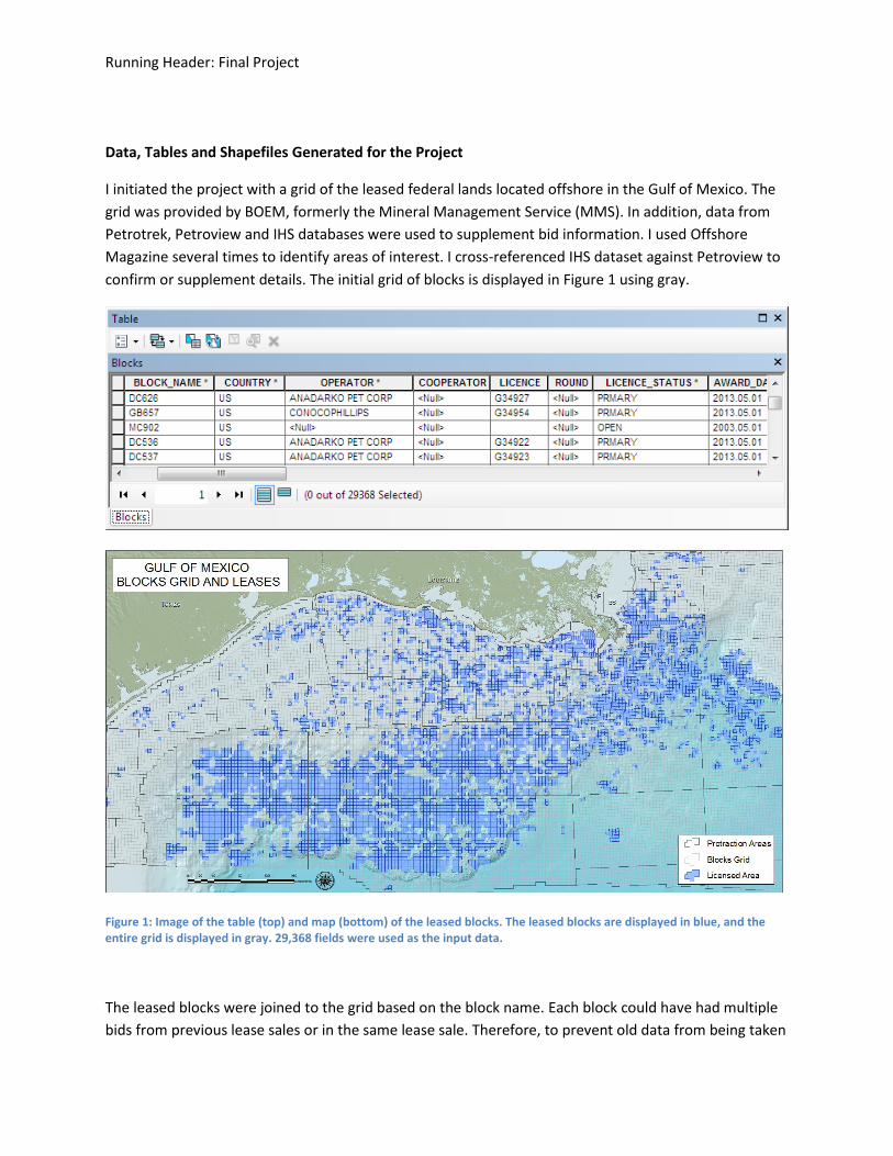
Data, Tables and Shapefiles Generated for the Project

I initiated the project with a grid of the leased federal lands located offshore in the Gulf of Mexico. The

grid was provided by BOEM, formerly the Mineral Management Service (MMS). In addition, data from

Petrotrek, Petroview and IHS databases were used to supplement bid information. I used Offshore

Magazine several times to identify areas of interest. I cross-referenced IHS dataset against Petroview to

confirm or supplement details. The initial grid of blocks is displayed in Figure 1 using gray.

Figure 1: Image of the table (top) and map (bottom) of the leased blocks. The leased blocks are displayed in blue, and the entire grid is displayed in gray. 29,368 fields were used as the input data.

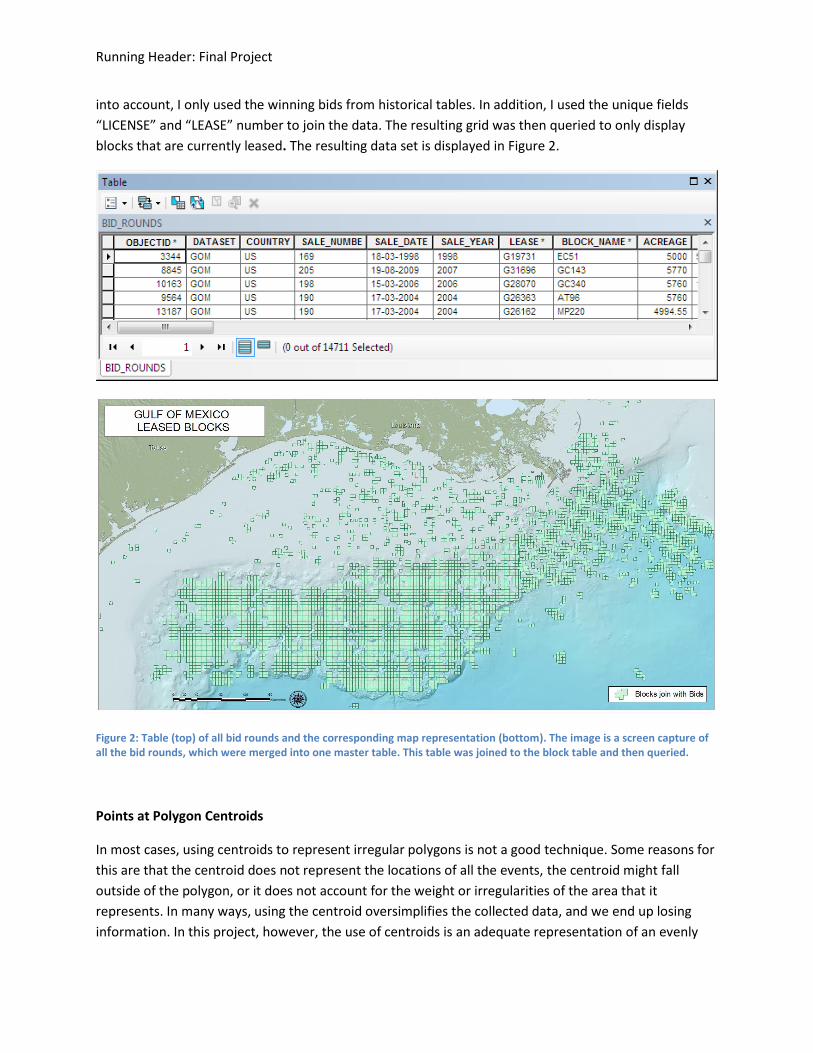
The leased blocks were joined to the grid based on the block name. Each block could have had multiple

bids from previous lease sales or in the same lease sale. Therefore, to prevent old data from being taken


into account, I only used the winning bids from historical tables. In addition, I used the unique fields

“LICENSE” and “LEASE” number to join the data. The resulting grid was then queried to only display

blocks that are currently leased. The resulting data set is displayed in Figure 2.

Figure 2: Table (top) of all bid rounds and the corresponding map representation (bottom). The image is a screen capture of all the bid rounds, which were merged into one master table. This table was joined to the block table and then queried.

Points at Polygon Centroids

In most cases, using centroids to represent irregular polygons is not a good technique. Some reasons for

this are that the centroid does not represent the locations of all the events, the centroid might fall

outside of the polygon, or it does not account for the weight or irregularities of the area that it

represents. In many ways, using the centroid oversimplifies the collected data, and we end up losing

information. In this project, however, the use of centroids is an adequate representation of an evenly


spaced grid of parallelograms that are in their majority identical in shape and size. As a consequence,

the use of centroids facilitates the analysis.

By knowing the data we are working with, we can make a representation using steps that help retain its

value and avoid creating a modifiable areal unit problem (MAUP) (O’Sullivan 2010). The data in this

study is distributed in a grid-like way, in which most of the blocks fall into two categories: the south

addition blocks and the deep water blocks. Their sizes are respectively 5,000 acres and 5,760 acres

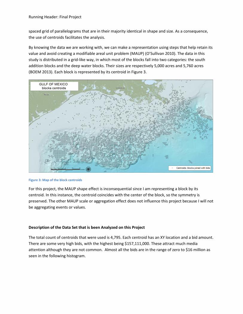
(BOEM 2013). Each block is represented by its centroid in Figure 3.

Figure 3: Map of the block centroids

For this project, the MAUP shape effect is inconsequential since I am representing a block by its

centroid. In this instance, the centroid coincides with the center of the block, so the symmetry is

preserved. The other MAUP scale or aggregation effect does not influence this project because I will not

be aggregating events or values.

Description of the Data Set that is been Analyzed on this Project

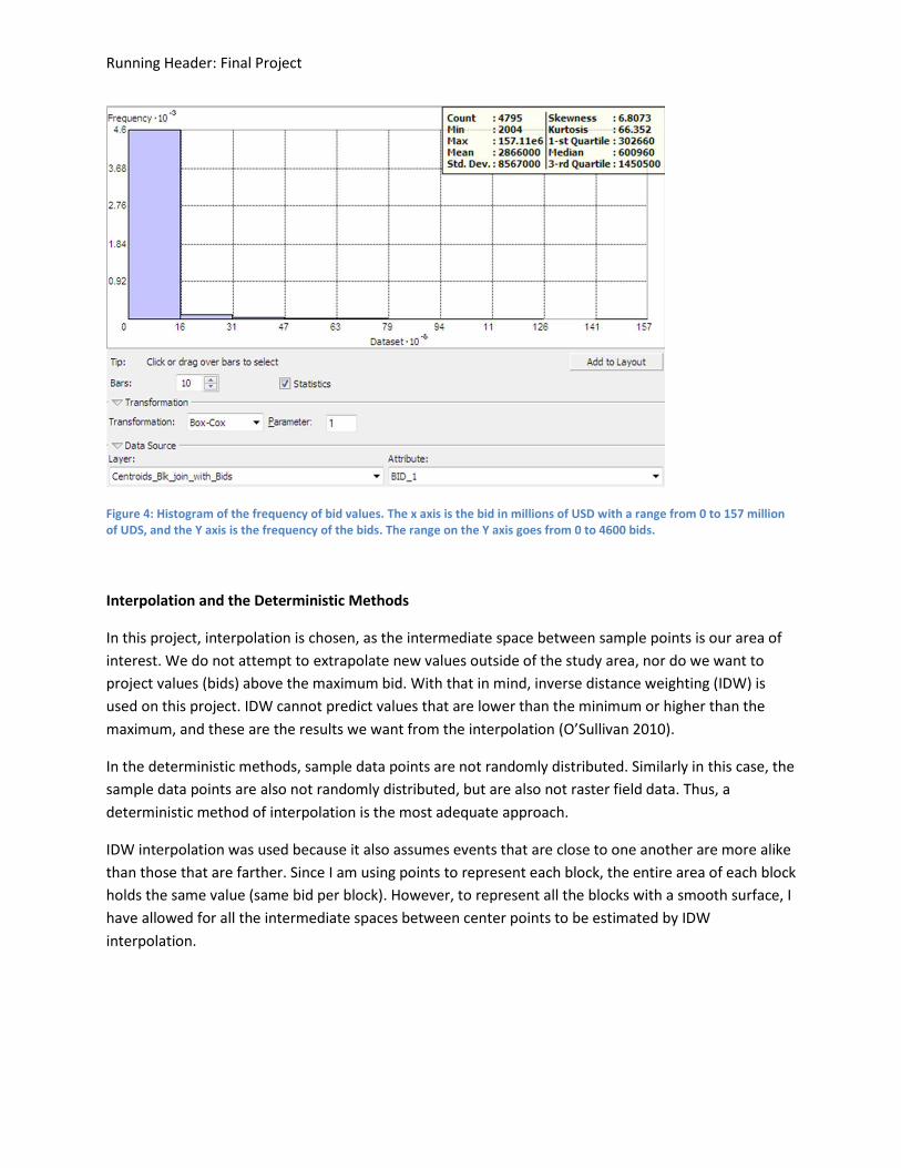
The total count of centroids that were used is 4,795. Each centroid has an XY location and a bid amount.

There are some very high bids, with the highest being $157,111,000. These attract much media

attention although they are not common. Almost all the bids are in the range of zero to $16 million as

seen in the following histogram.


Figure 4: Histogram of the frequency of bid values. The x axis is the bid in millions of USD with a range from 0 to 157 million of UDS, and the Y axis is the frequency of the bids. The range on the Y axis goes from 0 to 4600 bids.

Interpolation and the Deterministic Methods

In this project, interpolation is chosen, as the intermediate space between sample points is our area of

interest. We do not attempt to extrapolate new values outside of the study area, nor do we want to

project values (bids) above the maximum bid. With that in mind, inverse distance weighting (IDW) is

used on this project. IDW cannot predict values that are lower than the minimum or higher than the

maximum, and these are the results we want from the interpolation (O’Sullivan 2010).

In the deterministic methods, sample data points are not randomly distributed. Similarly in this case, the

sample data points are also not randomly distributed, but are also not raster field data. Thus, a

deterministic method of interpolation is the most adequate approach.

IDW interpolation was used because it also assumes events that are close to one another are more alike

than those that are farther. Since I am using points to represent each block, the entire area of each block

holds the same value (same bid per block). However, to represent all the blocks with a smooth surface, I

have allowed for all the intermediate spaces between center points to be estimated by IDW

interpolation.


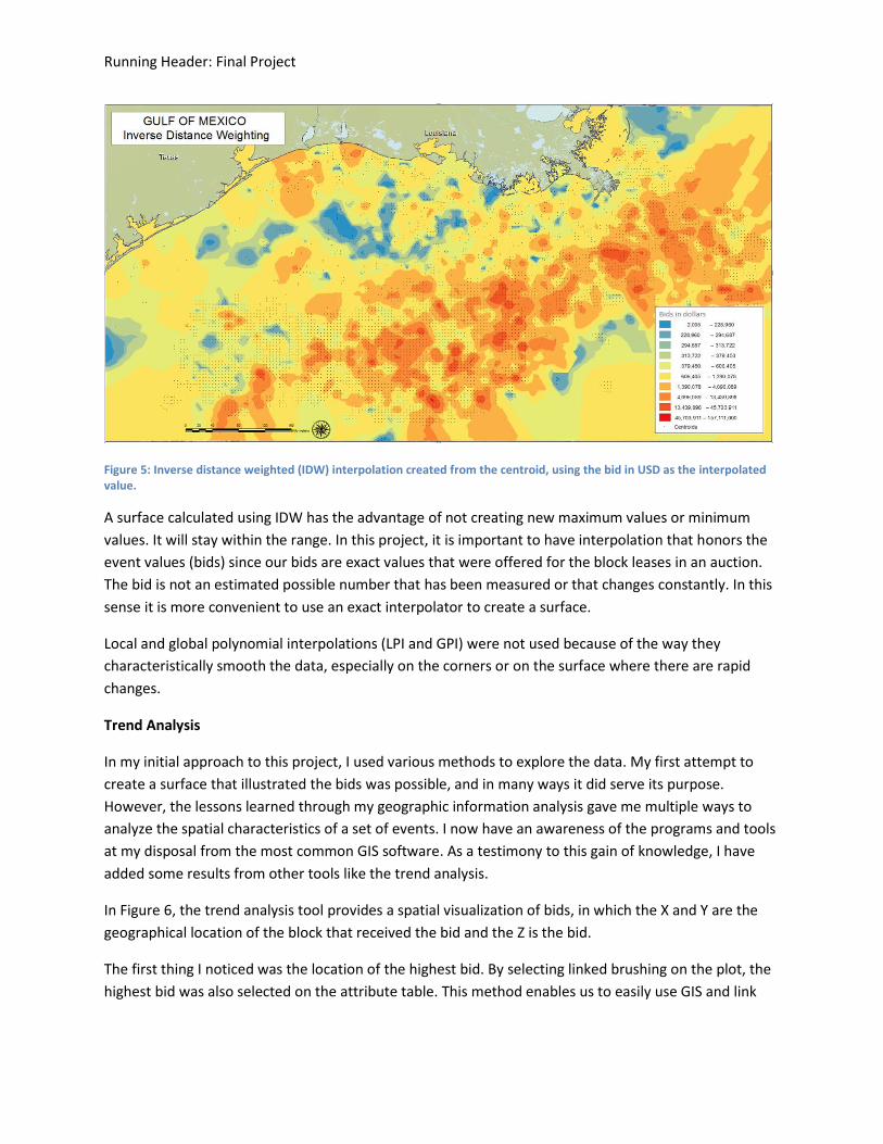
Figure 5: Inverse distance weighted (IDW) interpolation created from the centroid, using the bid in USD as the interpolated value.

A surface calculated using IDW has the advantage of not creating new maximum values or minimum

values. It will stay within the range. In this project, it is important to have interpolation that honors the

event values (bids) since our bids are exact values that were offered for the block leases in an auction.

The bid is not an estimated possible number that has been measured or that changes constantly. In this

sense it is more convenient to use an exact interpolator to create a surface.

Local and global polynomial interpolations (LPI and GPI) were not used because of the way they

characteristically smooth the data, especially on the corners or on the surface where there are rapid

changes.

Trend Analysis

In my initial approach to this project, I used various methods to explore the data. My first attempt to

create a surface that illustrated the bids was possible, and in many ways it did serve its purpose.

However, the lessons learned through my geographic information analysis gave me multiple ways to

analyze the spatial characteristics of a set of events. I now have an awareness of the programs and tools

at my disposal from the most common GIS software. As a testimony to this gain of knowledge, I have

added some results from other tools like the trend analysis.

In Figure 6, the trend analysis tool provides a spatial visualization of bids, in which the X and Y are the

geographical location of the block that received the bid and the Z is the bid.

The first thing I noticed was the location of the highest bid. By selecting linked brushing on the plot, the

highest bid was also selected on the attribute table. This method enables us to easily use GIS and link


some additional information to the data, such as the company that made the bid or the date of the bid.

Then we can estimate when the bid occurred and also analyze all the relevant time-related data.

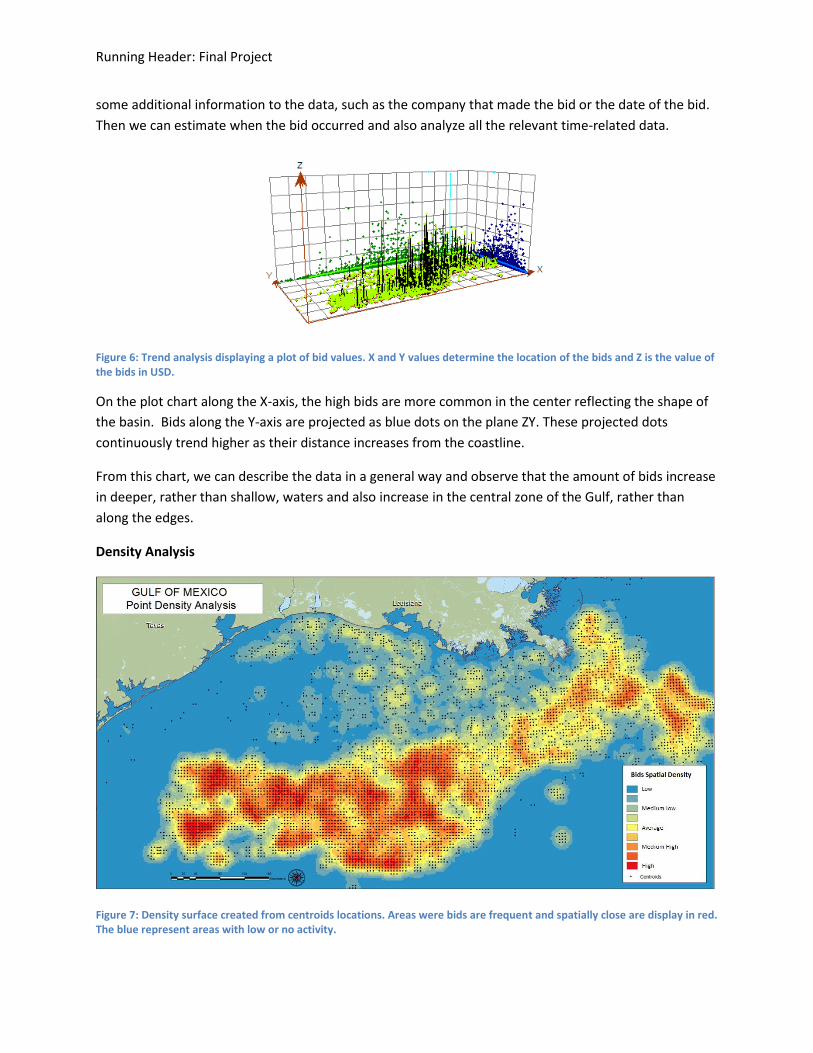
Figure 6: Trend analysis displaying a plot of bid values. X and Y values determine the location of the bids and Z is the value of the bids in USD.

On the plot chart along the X-axis, the high bids are more common in the center reflecting the shape of

the basin. Bids along the Y-axis are projected as blue dots on the plane ZY. These projected dots

continuously trend higher as their distance increases from the coastline.

From this chart, we can describe the data in a general way and observe that the amount of bids increase

in deeper, rather than shallow, waters and also increase in the central zone of the Gulf, rather than

along the edges.

Density Analysis

Figure 7: Density surface created from centroids locations. Areas were bids are frequent and spatially close are display in red. The blue represent areas with low or no activity.


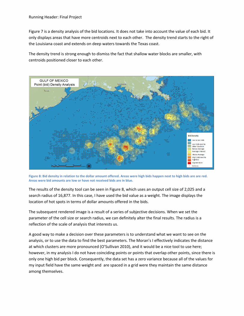
Figure 7 is a density analysis of the bid locations. It does not take into account the value of each bid. It

only displays areas that have more centroids next to each other. The density trend starts to the right of

the Louisiana coast and extends on deep waters towards the Texas coast.

The density trend is strong enough to dismiss the fact that shallow water blocks are smaller, with

centroids positioned closer to each other.

Figure 8: Bid density in relation to the dollar amount offered. Areas were high bids happen next to high bids are are red. Areas were bid amounts are low or have not received bids are in blue.

The results of the density tool can be seen in Figure 8, which uses an output cell size of 2,025 and a

search radius of 16,877. In this case, I have used the bid value as a weight. The image displays the

location of hot spots in terms of dollar amounts offered in the bids.

The subsequent rendered image is a result of a series of subjective decisions. When we set the

parameter of the cell size or search radius, we can definitely alter the final results. The radius is a

reflection of the scale of analysis that interests us.

A good way to make a decision over these parameters is to understand what we want to see on the

analysis, or to use the data to find the best parameters. The Moran’s I effectively indicates the distance

at which clusters are more pronounced (O’Sullivan 2010), and it would be a nice tool to use here;

however, in my analysis I do not have coinciding points or points that overlap other points, since there is

only one high bid per block. Consequently, the data set has a zero variance because all of the values for

my input field have the same weight and are spaced in a grid were they maintain the same distance

among themselves.


Further Analysis

After interpolating the surfaces from the filtered table and running the analysis tools, I can include all

the blocks, whether they had bids or not. In my current analysis, I have only included the blocks with

bids, so in a way I have ignored all the blocks without bids. For a future project, all the blocks with no

bids can be added and their bid fields can be populated with zeros to compare results.

This approach might cause us to wrongly consider the block value as zero. In addition, this assumption

might create an artificial deviation of the results. However the lease sale participants deemed these

blocks to be unworthy to bid on.

Additional Results and Conclusions:

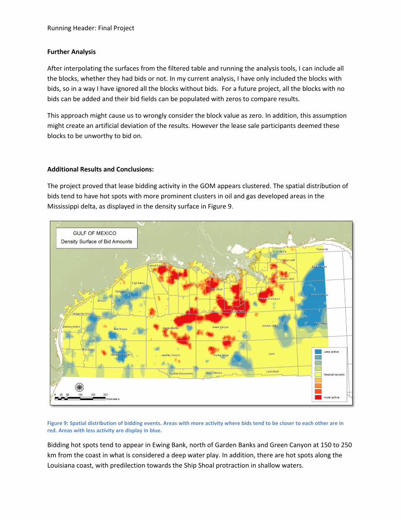
The project proved that lease bidding activity in the GOM appears clustered. The spatial distribution of

bids tend to have hot spots with more prominent clusters in oil and gas developed areas in the

Mississippi delta, as displayed in the density surface in Figure 9.

Figure 9: Spatial distribution of bidding events. Areas with more activity where bids tend to be closer to each other are in red. Areas with less activity are display in blue.

Bidding hot spots tend to appear in Ewing Bank, north of Garden Banks and Green Canyon at 150 to 250

km from the coast in what is considered a deep water play. In addition, there are hot spots along the

Louisiana coast, with predilection towards the Ship Shoal protraction in shallow waters.


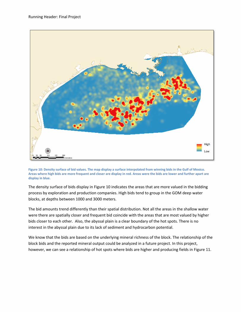
Figure 10: Density surface of bid values. The map display a surface interpolated from winning bids in the Gulf of Mexico. Areas where high bids are more frequent and closer are display in red. Areas were the bids are lower and further apart are display in blue.

The density surface of bids display in Figure 10 indicates the areas that are more valued in the bidding

process by exploration and production companies. High bids tend to group in the GOM deep water

blocks, at depths between 1000 and 3000 meters.

The bid amounts trend differently than their spatial distribution. Not all the areas in the shallow water

were there are spatially closer and frequent bid coincide with the areas that are most valued by higher

bids closer to each other. Also, the abyssal plain is a clear boundary of the hot spots. There is no

interest in the abyssal plain due to its lack of sediment and hydrocarbon potential.

We know that the bids are based on the underlying mineral richness of the block. The relationship of the

block bids and the reported mineral output could be analyzed in a future project. In this project,

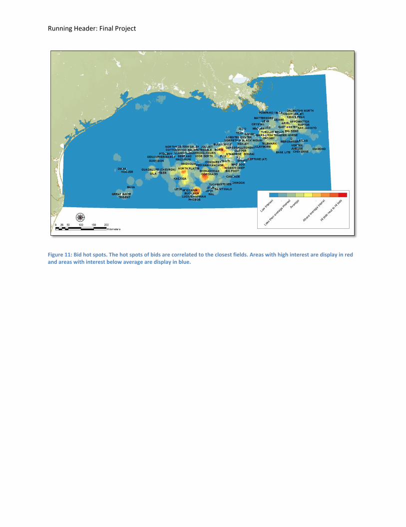
however, we can see a relationship of hot spots where bids are higher and producing fields in Figure 11.


Figure 11: Bid hot spots. The hot spots of bids are correlated to the closest fields. Areas with high interest are display in red and areas with interest below average are display in blue.


Sources

Bureau of Ocean Energy Management (2013), Status of Gulf of Mexico Plans. Retrieved December 7, 2013, from http://www.boem.gov/Status-of-Gulf-of-Mexico-Plans/

Crawford, Gerald T. (2008) "Estimated Oil and Gas Reserves Gulf of Mexico OCS Region." OCS Report BOEM

Fischer, Manfred M. (2009) Handbook of applied spatial analysis software tools, methods and applications.

Iledare, Omowumi Odeniyi (2015) "Profitability in Offshore Petroleum Leases: Empirical Evidence From the US Gulf of Mexico Deepwater Region." SPE Annual Technical Conference and Exhibition (2008). Web. 29 Sept. 2015.

Nomack, Mallory (2010) "Deepwater Gulf of Mexico Oil Reserves and Production." Deepwater Gulf of Mexico Oil Reserves and Production. Ed. Cutler J Cleveland. The Encyclopedia of the Earth, 24 Sept. 2010. Web. 14 Oct. 2015.

O’Sullivan, David and Unwin, David J. (2010). Geographic Information Analysis 2nd ed. Retrieved

December 8, 2013.

Tavares, Mario (2000) "Bidding Strategy: Reducing the "Money-Left-on-the-Table" in E&P Licensing Opportunity." Proceedings of SPE Annual Technical Conference and Exhibition (2000). Web. 29 Sept. 2015.

U.S. Bureau of the Census (n.d.).American FactFinder. Retrieved December 7, 2013 from http://factfinder2.census.gov

bidding tendencies in the gulf of mexico · bidding tendencies in the gulf of mexico ... bids along...

Documents