bicycling suitability in downtown, cairo, egypt · cairo, the capital of egypt is considered as one...
TRANSCRIPT
Master Thesis in Geographical Information Science nr 60
Karim Alaa El Din Mohamed Soliman El Attar
2016
Department of
Physical Geography and Ecosystem Science
Centre for Geographical Information Systems
Lund University
Sölvegatan 12
S-223 62 Lund
Sweden
Bicycling Suitability in Downtown, Cairo, Egypt

ii
Author: Karim Alaa El Din Mohamed Soliman El Attar. Title: Bicycling Suitability in Downtown, Cairo, Egypt. Master degree thesis, 30/ credits in Master in Geographical Information Sciences Department of Physical Geography and Ecosystem Science, Lund University
iii
Bicycling Suitability in Downtown, Cairo, Egypt
Karim A. El Attar
Master thesis, 30 credits, in Geographical Information Sciences
Vaughan Phillips Lund University
Supervisor
Amr H. Ali Benha University
Co-Supervisor

iv
Dedication
At the beginning, I would like to thank God, for supporting me during the Master’s
Degree journey and for giving me the ability to complete this thesis.
Many thanks to my family especially my wife Dina and my kids Yahia and Yasin for
their understanding and support during the Master’s journey that took me away from
them for a long time. A special thanks to my best friend, Ahmed Makram.
I would like to send a special dedication to the soul of my father Hossam Khairat who
died before completing this Degree. He encouraged and supported me in all possible
ways; I wish he were with me now.

v
Acknowledgment
A very special thanks and appreciation to my supervisor Dr. Vaughan Philips,
Department of Physical Geography and Ecosystem Science, LUND University for his
kindness and valuable support, and providing the expert guidance. Special thanks also to
Dr. Amr Ali for his valuable suggestions and discussions throughout the LUMA program
as a co-supervisor for this research. Also, I would like to thank Eng. Heba El Kady for
her great support.
I wish to express my gratitude to Dr. Ulrik Mårtensson, Dr. Micael Runnstöm and Dr.
Petter Pilesjö for their assistance throughout LUMA program.
Finally, I would like to thank LUND University-GIS Centrum team for their support
during the whole Master’s journey.
Karim El Attar
vi
Abstract
The Greater Cairo is one of the most crowded cities in the world and it is the
biggest metropolitan area in Middle East. The high population density in the Greater
Cairo causes traffic problems that harm many living aspects. This study discusses one of
the solutions for limiting the traffic congestions using bicycle as an alternative
transportation mean which is already applied in many other countries.
There are many models have been introduced to study the suitability of having
bicyclists on a motor road. This study will apply some of the most commonly used
models created to measure bicycling suitability.in Down Town Cairo area.
A GIS tool has been created to conduct applying the bicycling suitability models
on the study area’s streets. The tool was developed in ArcMap using Microsoft Visual
Studio.
The results of this study encourage having alternative transportation network for
bicycles in Down Town Cairo. The tool created is a user-friendly tool and it could be
used for other researches in different areas or countries.
vii
Table of Contents List of Figures ................................................................................................................................... ix
List of Tables .................................................................................................................................... ix
List of Equations ............................................................................................................................... x
List of Abbreviations ........................................................................................................................ xi
1 Introduction ............................................................................................................................. 1
1.1 Problem definition ........................................................................................................... 1
1.2 Objectives ........................................................................................................................ 2
Proposed method .................................................................................................... 2 1.2.1
1.3 Research Questions ......................................................................................................... 2
2 Study Area ............................................................................................................................... 3
2.1 Geographic Location ........................................................................................................ 3
2.2 Historical Importance ...................................................................................................... 4
2.3 Economic Importance ...................................................................................................... 4
2.4 Population ....................................................................................................................... 4
2.5 Cairo................................................................................................................................. 5
2.6 Downtown ....................................................................................................................... 5
2.7 Cycling in Egypt ................................................................................................................ 6
3 Literature Review .................................................................................................................... 9
3.1 Theoretical Approaches ................................................................................................... 9
Egypt’s Infrastructure and Road Network ............................................................... 9 3.1.1
Traffic congestion in Cairo ....................................................................................... 9 3.1.2
Why Downtown? ................................................................................................... 10 3.1.3
Bicycle as an indispensable transportation mean ................................................. 14 3.1.4
Co-benefits of Cycling ............................................................................................ 14 3.1.5
Factors Affecting Cycling ....................................................................................... 15 3.1.6
Previous studies about planning a Cycling network .............................................. 16 3.1.7
Common Methods, Theories and Models ............................................................. 21 3.1.8
3.2 Technical Approaches .................................................................................................... 37
What is GIS? ........................................................................................................... 37 3.2.1
GIS Applications ..................................................................................................... 37 3.2.2
4 Data Required ........................................................................................................................ 39
viii
4.1 Geometry ....................................................................................................................... 39
4.2 Attributes ....................................................................................................................... 39
4.3 Data Description ............................................................................................................ 40
4.4 Sources of the Data ....................................................................................................... 45
4.5 Received Data ................................................................................................................ 46
Geometry ............................................................................................................... 46 4.5.1
Traffic Volumes ...................................................................................................... 47 4.5.2
Speed Limits........................................................................................................... 49 4.5.3
Street Lanes Attributes .......................................................................................... 49 4.5.4
5 Methodology and Analysis .................................................................................................... 51
5.1 Introduction ................................................................................................................... 51
5.2 Bicycle Suitability Methodologies ................................................................................. 51
5.3 Data Preparation ........................................................................................................... 52
5.4 The Bicycle Suitability Modelling Tool ........................................................................... 53
6 Results and Analysis .............................................................................................................. 57
6.1 Bruce Epperson Modified Roadway Condition Index .................................................... 57
6.2 Petritsch’s BLOS ............................................................................................................. 61
6.3 Bicycle Compatibility Index (Harkey) ............................................................................. 64
6.4 Bicycle Level of Service (HCM)....................................................................................... 68
6.5 Discussion ...................................................................................................................... 71
7 Conclusions ............................................................................................................................ 73
7.1 Future Work .................................................................................................................. 74
7.2 Recommendations ......................................................................................................... 74
8 References ............................................................................................................................. 75
9 Appendices ............................................................................................................................ 81
9.1 Appendix A .................................................................................................................... 81
ix
List of Figures Figure 1 Egypt Map from the official web site of GIZA governorate (www.giza.gov.eg) 3
Figure 2 European Style Buildings, downtown Cairo (Berthold Werner, 2010) ................ 5
Figure 3 Borders of Cairo Downtown area (Hassan , Lee & Yoo, 2014) ........................... 6
Figure 4 Ground and first storey use of the Cairo downtown area (Hassan , Lee & Yoo, 2014) ................................................................................................................................. 11
Figure 5 Pedestrians are exposed to motor vehicle emissions in Downtown (El Araby, 2002) ................................................................................................................................. 12
Figure 6 A Map illustrates the no-parking streets in downtown area (Awatta, 2015) ...... 13
Figure 7 Flow chart of the Procedure (Huang & Ye, 1995) ............................................. 17
Figure 8 Bicycle Level Of service and DEMAND cluster maps (Rybarczyk & Wu, 2010)........................................................................................................................................... 18
Figure 9 Display for the prioritization index applied on the Island of Montreal (Larsen , Patterson & El-Geneidy, 2013) ......................................................................................... 20
Figure 10 Street Lanes (Harkey , Reinfurt & Sorton, 1998) ............................................. 43
Figure 11 Data Sources ..................................................................................................... 45
Figure 12 Downtown Geometry (Source: Benha University) .......................................... 46
Figure 13 Adding the Add-In to the ArcMap ................................................................... 54
Figure 14 Displayed icons for the Bicycling Suitability Modelling Tool ........................ 54
Figure 15 Bicycling Suitability Modelling Interface ........................................................ 55
Figure 16 Bicycling Suitability Modelling Interface - Unit Conversion function ............ 55
Figure 17 Columns generated via the Bicycling Suitability Modelling tool and the sympology map that could be created using them ............................................................ 56
Figure 18 Chart illustrates Bruce Epperson Modified Roadway Condition Index KMs/Index Class ............................................................................................................... 57
Figure 19 Bruce Epperson Modified Roadway Condition Index applied on Downtown area .................................................................................................................................... 60
Figure 20 Chart illustrates Petritsch’s BLOS KMs/Index Class ....................................... 61
Figure 21 Petritsch’s BLOS Model applied on Downtown area ...................................... 63
Figure 22 Chart illustrates BCI KMs/Index Class ............................................................ 64
Figure 23 BCI Model applied on Downtown area ............................................................ 67
Figure 24 Chart illustrates HCM BLOS KMs/Index Class .............................................. 68
Figure 25 HCM BLOS Model applied on Downtown area .............................................. 70
Figure 26 All Models Applied Results Comparison ......................................................... 71
List of Tables Table 1 1997–2000 Jersey City Bicycle Crash Severity Index Distribution (Allen-Munley & Daniel, 2006) ................................................................................................................ 21
Table 2 Common Bicycle Suitability Methods (Lowry , Callister , Gresham & Moore, 2012) ................................................................................................................................. 22
Table 3 Bicycle Suitability/Safety/LOS Methodologies Affecting Factors (Turner , Shafer & Stewart, 1997) ............................................................................................................... 23
Table 4 Interpretation of Bicycle Suitability Scores (Turner , Shafer & Stewart, 1997) . 29
Table 5 BCI Adjustment factors ....................................................................................... 33
Table 6 BCI ranges associated with LOS Designations and Qualifiers (Harkey , Reinfurt , Knuiman , Stewart & Sorton, 1998) ................................................................................. 34
x
Table 7 Roadway Attributes for Selected Bicycle Suitability Methods (Callister & Lowry, 2013) ................................................................................................................................. 34
Table 8 Levels of Traffic Stress (LTS) (Mekuria , Furth & Nixon, 2012) ....................... 36
Table 9 Traffic peak periods in the Greater Cairo Metropolitan Area (World Bank, 2013)........................................................................................................................................... 42
Table 10 Urban Roads Specifications in Egypt (The Egyptian Code of Practice) ........... 44
Table 11 Downtown Attributes (Source: Benha University) ............................................ 47
Table 12 Gomhuria Street and Abd El Khalik Tharwat Street (Source: Ain Shams University) ........................................................................................................................ 48
Table 13 The applied Methods and Factors ...................................................................... 51
Table 14 Field Sheet to facilitate the field measurements ................................................ 52
Table 15 Bruce Epperson Modified Roadway Condition Index KM covered per Index Class .................................................................................................................................. 57
Table 16 Bruce Epperson Modified Roadway Condition Index Class' KMs covered per Street Name ....................................................................................................................... 58
Table 17 Petritsch’s BLOS KM covered per Index Class ................................................ 61
Table 18 Petritsch’s BLOS Index Class' KMs covered per Street Name ......................... 62
Table 19 BCI KM covered per Index Class ...................................................................... 64
Table 20 BCI Index Class' KMs covered per Street Name ............................................... 65
Table 21 HCM BLOS KM covered per Index Class ........................................................ 68
Table 22 HCM BLOS Index Class' KMs covered per Street Name ................................. 69
Table 23 Average results per Street Name per Model and General suitablity score ........ 72
List of Equations Equation 1 The prioritization index equation (Larsen , Patterson & El-Geneidy, 2013) . 19
Equation 2 (RSI) and (IEI) Equations (Epperson, 1994) .................................................. 24
Equation 3 Epperson-Davis RCI (Turner , Shafer & Stewart, 1997) ............................... 25
Equation 4 Modified RCI (Epperson, 1994) ..................................................................... 26
Equation 5 Interaction Hazard Score (IHS) Equation (Landis, 1994) .............................. 26
Equation 6 Landis’ Bicycle Level of Service Model (The update) (Turner , Shafer & Stewart, 1997) ................................................................................................................... 27
Equation 7 Bicycle Suitability Score Equation (Turner , Shafer & Stewart, 1997) ......... 28
Equation 8 Jensen BLOS Model (Jensen, 2007) .............................................................. 30
Equation 9 Bicycle Segment LOS (, 2007) ....................................................................... 31
Equation 10 Bicycle Facility LOS (, 2007) ...................................................................... 32
Equation 11 Bicycle Compatibility Index Model (Harkey , Reinfurt , Knuiman , Stewart & Sorton, 1998) ................................................................................................................ 32
Equation 12 BLOS Perception Index (Callister & Lowry, 2013) ..................................... 35
Equation 13 Peak Hour Volume Equation (Harkey , Reinfurt , Knuiman , Stewart & Sorton, 1998)..................................................................................................................... 41
xi
List of Abbreviations AADT: Average Anual daily Traffic. ADT: Average daily traffic. BCI: Bicycle Compatability Idex. BLOS: Bicycle level of service. BSA: Sicycle Suitability Assessment. BSIR: Bicycle Suitability Score Index. BSL: Bicycle Stress Level. BSS: bicycle Suitability Score. HCM: Highway capacity manual. LTS: Level of Traffic Stress. RCI: Road Condition Index.

xii
1
1 Introduction
The city of Cairo, Egypt is ranked as the 42nd most crowded city in the world, with
around 12 Million inhabitants and a density of about 1540/sq. km (Maps of World, 2015).
5.854 million Vehicles are registered in Egypt 31.6 percent of which exist in Cairo only
with an ownership rate of over 20/100 people (Ahram Online, 2011). Over 1.2 million
vehicles are registered in Greater Cairo only, with an annual incremental rate of 10% (Ali
& Tamura, 2002) especially through Down Town, where most of the ministries,
governmental institutions, banks, and local or private companies are located.
President Abd el Fattah El Sisi has recently started encouraging cycling by showing
up at many events riding a bicycle. Even during his presidential campaign before the
elections; the co-founder of Cairo Cycler’s Club commented on Sisi’s cycling activities,
saying that the sunny weather and suitable topographic nature make Cairo an attractive
place for cyclists (Kingsley, 2014). Cycling has become a trend in Egypt in the recent
years, as there are now multiple groups and parties that could be found on social media
managing cycling events during the year (Rabie, 2015).
On an international level, many directed strategies aim to use sustainable transport
means that are safe, clean and affordable. In addition to being an economic, safe, and
healthy mean of transport, the bicycle contributes to the reduction of polluting emissions
(World Bank, 2008).
1.1 Problem definition
Cairo, the capital of Egypt is considered as one of the most crowded cities in the
world. Down Town, Cairo suffers from traffic jams and many other problems. It is a
historical area that is full of museums, banks, governmental offices, shopping spots and site
scenes.
Riding bicycles is not a common behavior in the Egyptian culture. However, in the
past few years, a trend has developed among the young generation to use bicycles instead
of other transportation means. Unfortunately, the road network infrastructure is not ready
for such kind of means.
Establishing a bicycle route network in the downtown area will contribute to
decreasing the traffic jams and pollution problems, as the new network would encourage
2
inhabitants and visitors to ride bicycles instead of other motorized means. Down Town
streets’ features and dimensions need to be studied to determine the best fit ways for the
bicycle route network through applying known methodologies and models of the bicycle
level of service and compatibility to help the decision maker select the suitable streets for
the new users’ segment.
1.2 Objectives
The aim of this research project is to use Arc GIS in testing the bicycle suitability
models to establish a route network for cycling in Down Town Cairo for the purpose of
traffic reduction and to support an alternative mean of transportation in Egypt.
Proposed method 1.2.1
The proposed method is to use GIS capabilities in planning the cycling route network
in Downtown, Cairo with respect to factors chosen based on the current situation in the
study area and similar projects applied in other countries – listed as following:
1- Road Bicycle Level of Service (BLOS) or Compatibility.
2- Traffic (speed, function class, number of points of interest) – sourcing from
educational/governmental authorities.
3- Road Characteristics (width, number of lanes, type and condition of pavement,
number of intersections) – Field data collection.
1.3 Research Questions
Research questions are the main lead for the hypotheses of this resreach so the
questions listed below are being asked all the time while writting this thesis.
- Do Egypt need a cycling network? Why?
- What is the applicability of establishing a cycling routes network in Egypt?
- Is cycling a solution for reducing traffic?
- Is cycling a trend in Egypt?
- Who would use bicycle as a transportation mean?
- How GIS would help in establishing Cycling Routes network?
3
2 Study Area
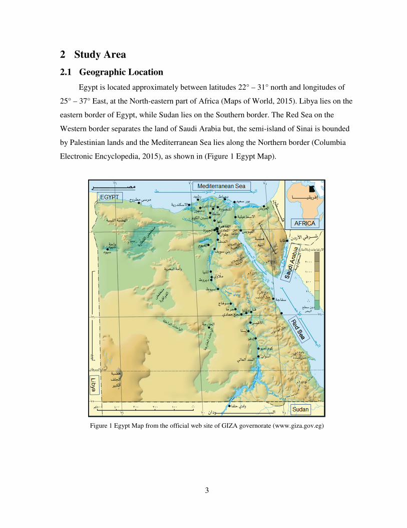
2.1 Geographic Location
Egypt is located approximately between latitudes 22° – 31° north and longitudes of
25° – 37° East, at the North-eastern part of Africa (Maps of World, 2015). Libya lies on the
eastern border of Egypt, while Sudan lies on the Southern border. The Red Sea on the
Western border separates the land of Saudi Arabia but, the semi-island of Sinai is bounded
by Palestinian lands and the Mediterranean Sea lies along the Northern border (Columbia
Electronic Encyclopedia, 2015), as shown in (Figure 1 Egypt Map).
Figure 1 Egypt Map from the official web site of GIZA governorate (www.giza.gov.eg)
4
The Nile River, which is the longest river on Earth, traverses Egypt Longitudinally.
Herodotus, a Greek historian, said ‘’Egypt is a gift of the Nile’’ – in other words, the Nile
River is the main source of water for agriculture and drinking in Egypt (Adams, 2007).
2.2 Historical Importance
Egypt is the land of the second oldest civilization after Sumerians: the Pharaohs. Not
only did they build the oldest standing structure, the Great Pyramid, which was made for
the Pharaoh “Khufu” they also preserved Pharaohs’ bodies with a mysterious process
known as mummification (Maps of World, 2015).
2.3 Economic Importance
Egypt roles Suez Canal that links between Mediterranean Sea to the Red Sea that
represents the shortest water path from Atlantic Ocean to the Indian Ocean by saving about
7000 KM between Europe and India (Suez Canal Authority, 2008). The GDP of Egypt
contributes 0.46% to the world economy, and its growth rate has been increasing over the
last 10 years, to reach a peak of 7.3%. Thus, Egypt is considered as one of the significant
developing countries in Middle East and Africa (Trading Economics, 2015).
2.4 Population
Egypt is the densest Arab country in the Middle East in terms of population, with
about 1540 per kilometer squared, its population exceeds 90 million (Maps of World,
2015); Egypt is divided/categorized into two regions – Upper Egypt, which includes rural
areas nearby the Sudanese borders in the south, and Lower Egypt in the south which covers
the Nile delta and cities by the Mediterranean shore including the capital, Cairo (Samari &
Pebley, 2015). 75% of Egypt’s population lives in Lower Egypt (Handoussa, 2008).
The prevailing religions in the country are Islam and Christianity, and the official
language is Arabic (Maps of World, 2015) . Furthermore, according to 2006 census data,
around 25% of the population is under 29 years (Handoussa, 2010).
5
2.5 Cairo
Cairo, Egypt’s capital is the largest metropolitan city in Africa and is ranked as the
13th largest mega city across the world (Huzayyin & Salem, 2013).Cairo’s population
exceeds 22% of the total Egyptian population; thus it suffers from serious traffic problems
that affect the economy negatively (World Bank, 2013).
2.6 Downtown
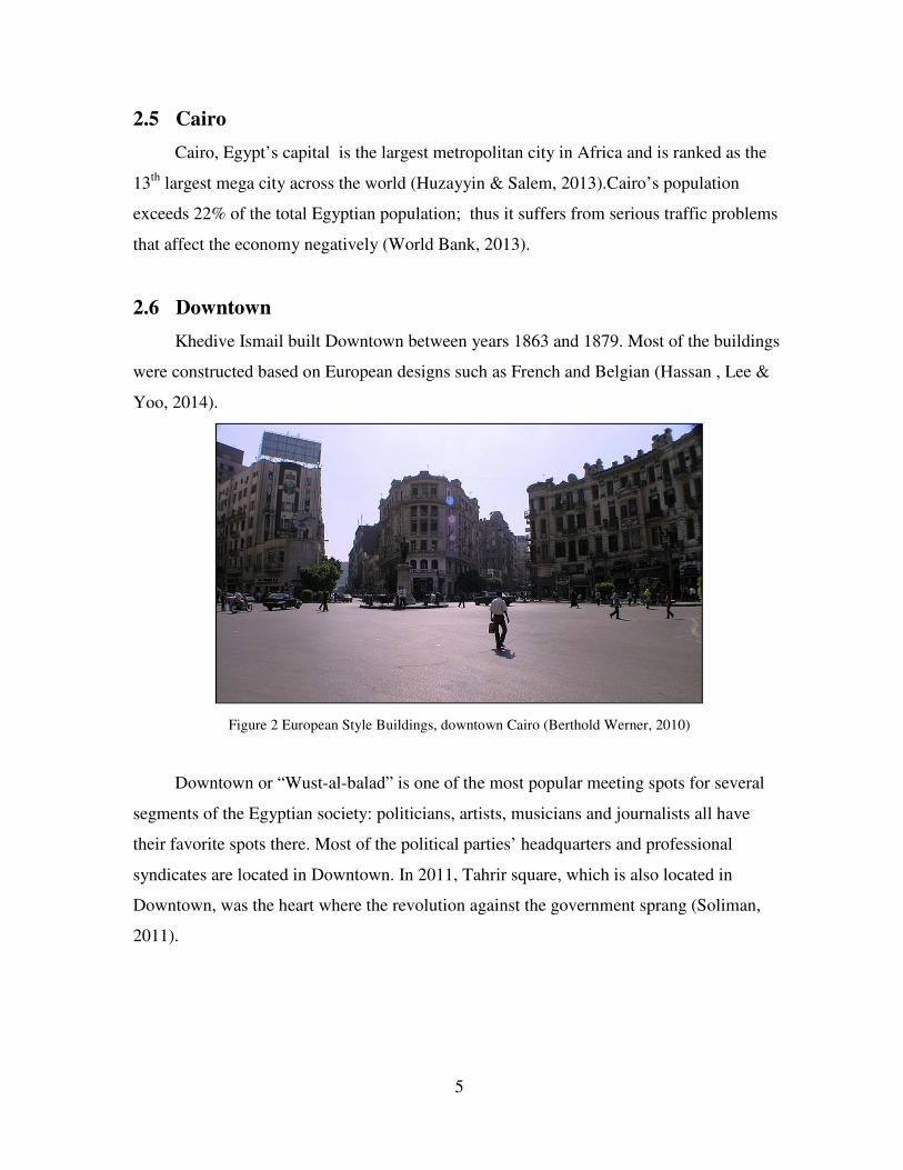
Khedive Ismail built Downtown between years 1863 and 1879. Most of the buildings
were constructed based on European designs such as French and Belgian (Hassan , Lee &
Yoo, 2014).
Figure 2 European Style Buildings, downtown Cairo (Berthold Werner, 2010)
Downtown or “Wust-al-balad” is one of the most popular meeting spots for several
segments of the Egyptian society: politicians, artists, musicians and journalists all have
their favorite spots there. Most of the political parties’ headquarters and professional
syndicates are located in Downtown. In 2011, Tahrir square, which is also located in
Downtown, was the heart where the revolution against the government sprang (Soliman,
2011).
6
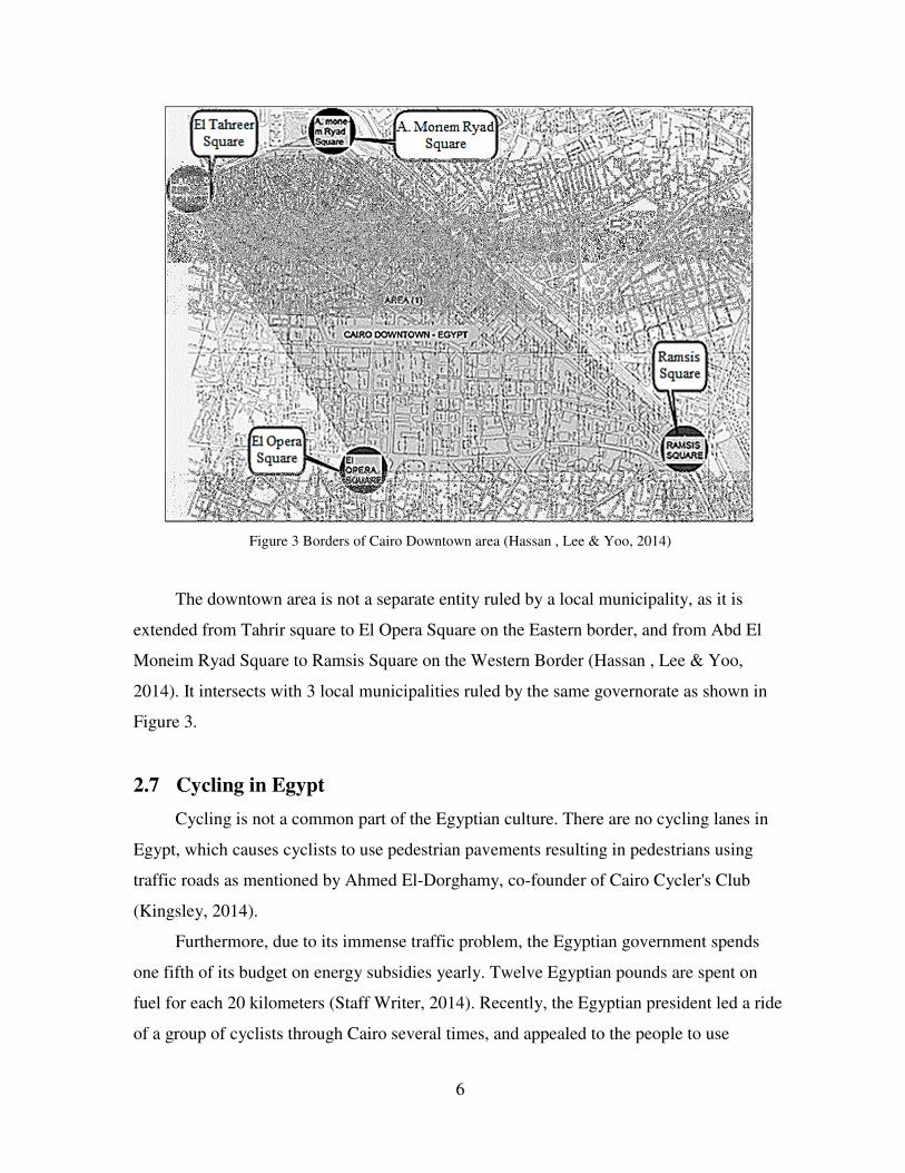
Figure 3 Borders of Cairo Downtown area (Hassan , Lee & Yoo, 2014)
The downtown area is not a separate entity ruled by a local municipality, as it is
extended from Tahrir square to El Opera Square on the Eastern border, and from Abd El
Moneim Ryad Square to Ramsis Square on the Western Border (Hassan , Lee & Yoo,
2014). It intersects with 3 local municipalities ruled by the same governorate as shown in
Figure 3.
2.7 Cycling in Egypt
Cycling is not a common part of the Egyptian culture. There are no cycling lanes in
Egypt, which causes cyclists to use pedestrian pavements resulting in pedestrians using
traffic roads as mentioned by Ahmed El-Dorghamy, co-founder of Cairo Cycler's Club
(Kingsley, 2014).
Furthermore, due to its immense traffic problem, the Egyptian government spends
one fifth of its budget on energy subsidies yearly. Twelve Egyptian pounds are spent on
fuel for each 20 kilometers (Staff Writer, 2014). Recently, the Egyptian president led a ride
of a group of cyclists through Cairo several times, and appealed to the people to use

7
bicycles as an indispensable transportation mean that will result in saving a noticeable part
of energy spending (Kingsley, 2014).

8
9
3 Literature Review
3.1 Theoretical Approaches
Egypt’s Infrastructure and Road Network 3.1.1
Egypt has languid road infrastructures caused by unplanned operations and lack of
tactical management (Semeida, 2013). One of the major road network problems in Egypt is
the lack of secondary roads that connect between main roads and the heart of the city; for
example, the Down Town area (El Araby, 2002).
Around 31 thousand kilometers of paved roads in good condition exist in Egypt,
connecting main cities with in the areas of the Nile Delta and Nile valley. However, a lack
of road markings and international standards is obvious on Egyptian highways. Main roads
are not sufficient for pedestrians in urban areas, as almost 50% of road accidents occur on
the roads maintained by the local authorities. Road signs follow European standards on
main roads only. Safety procedures such as emergency phones, traffic lights, and reflectors
are fairly widespread on highways unlike on secondary roads. Speed bumps are scattered
without planning and are barely marked. A non-safe driving environment prevails
throughout the street network due to the diversified and unrelated traffic mix that consists
of donkey carts, motorized tricycles, heavy trucks, busses, taxis, private vehicles and
minibuses (Association For safe International Road Travel, 2009).
The road fatality rates in the U.S. and UK are 0.9 and 0.7 respectively per 100-
kilometers, while in Egypt, rates reach 43.2, which is extremely high (Association For safe
International Road Travel, 2009). About 9608 deaths occurred in 2013 on Egypt’s roads, as
reported by the World Health Organization (Exelby, 2014).
Traffic congestion in Cairo 3.1.2
Traffic problems are caused by the increasing rate of owned vehicles registered in
Cairo, specifically 1.2 million, with an increasing ownership rate of 10% (Ali & Tamura,
2002). About 4.2 million vehicles move daily in streets that have an actual capacity of
500,000 vehicles only (Association For safe International Road Travel, 2009). This volume
of traffic congestion in Cairo actually costs the government about 8 billion USD annually,
which represents about 4% of the total Gross Domestic Product of Egypt (Exelby, 2014).
10
The Greater Cairo Metropolitan Region is considered as one of the worst cities with respect
to traffic (El Araby, 2002).
Around 59% of traffic problems are due to bad driving behaviour, including horn use,
wrong way driving, driving without focus, non-maintained vehicles, breaking speed rules,
and lack of lane commitment. (Ali & Tamura, 2002)
The Egyptian government started to plan and execute mega projects such as ring
road, new bridges and satellite cities surrounding greater Cairo, in order to try and handle
the rapidly increasing rate of private car ownership (World Bank, 2013).
There are solutions not that might not be considered mega projects, but will positively
affect the traffic situation, such as increasing the number of public buses, preventing side
parking in heavily crowded areas or at least during rush hours, carpooling, and toll-roads
(El Araby, 2002). Public transports serve over 60% of people’s daily trips in Greater Cairo
(World Bank, 2013).
Why Downtown? 3.1.3
The downtown area is mainly full of commercial stores, banks, headquarters, and
governmental offices; in addition to universities, institutes, schools, and tourist attraction
spots. As a result, there are employees, workers, students, shoppers, and tourists who
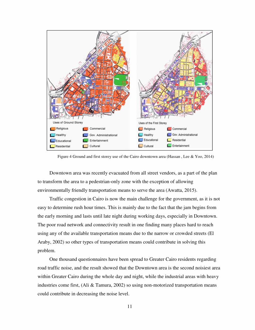
frequently visit Downtown (Hassan , Lee & Yoo, 2014)and (Laura, 2011). Figure 4
illustrates the land use coverage for the ground and first storeys in the Downtown Area:
11
Figure 4 Ground and first storey use of the Cairo downtown area (Hassan , Lee & Yoo, 2014)
Downtown area was recently evacuated from all street vendors, as a part of the plan
to transform the area to a pedestrian-only zone with the exception of allowing
environmentally friendly transportation means to serve the area (Awatta, 2015).
Traffic congestion in Cairo is now the main challenge for the government, as it is not
easy to determine rush hour times. This is mainly due to the fact that the jam begins from
the early morning and lasts until late night during working days, especially in Downtown.
The poor road network and connectivity result in one finding many places hard to reach
using any of the available transportation means due to the narrow or crowded streets (El
Araby, 2002) so other types of transportation means could contribute in solving this
problem.
One thousand questionnaires have been spread to Greater Cairo residents regarding
road traffic noise, and the result showed that the Downtown area is the second noisiest area
within Greater Cairo during the whole day and night, while the industrial areas with heavy
industries come first, (Ali & Tamura, 2002) so using non-motorized transportation means
could contribute in decreasing the noise level.
12
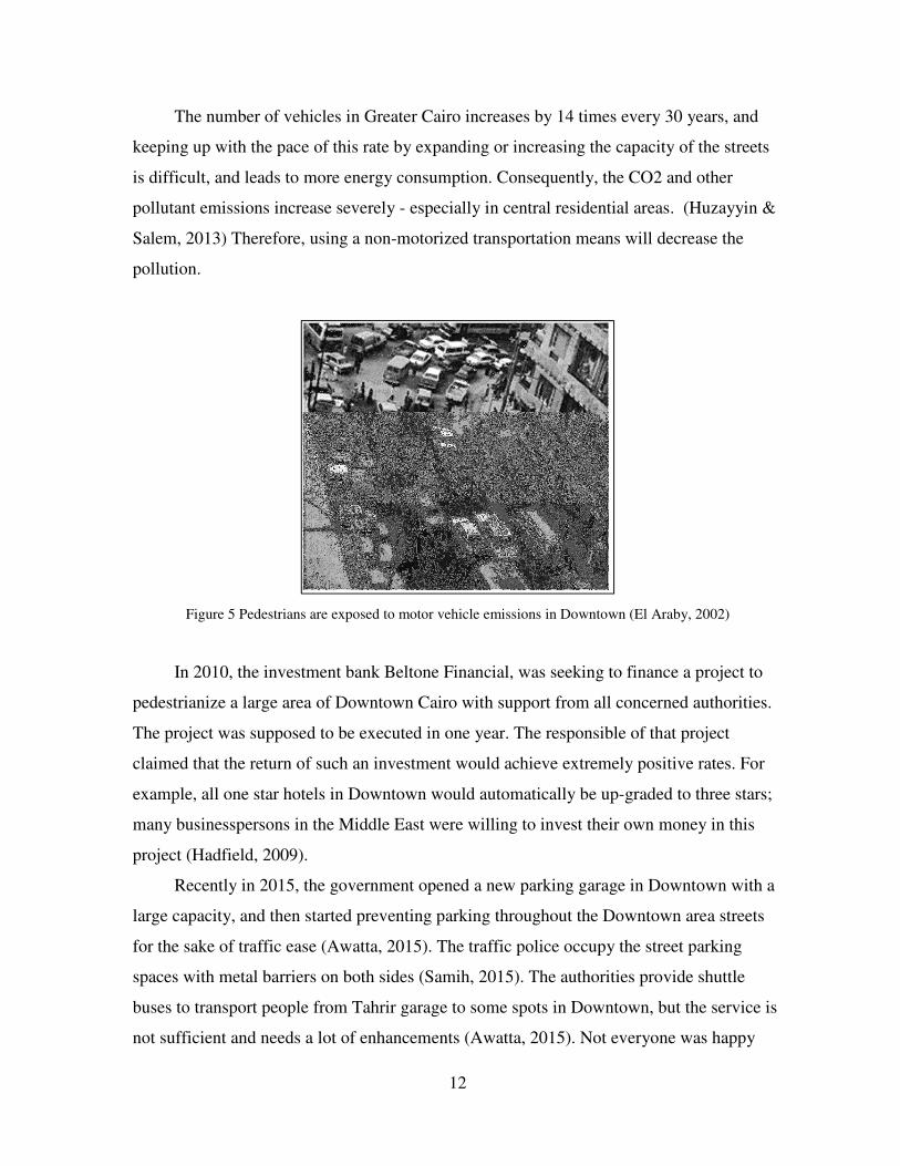
The number of vehicles in Greater Cairo increases by 14 times every 30 years, and
keeping up with the pace of this rate by expanding or increasing the capacity of the streets
is difficult, and leads to more energy consumption. Consequently, the CO2 and other
pollutant emissions increase severely - especially in central residential areas. (Huzayyin &
Salem, 2013) Therefore, using a non-motorized transportation means will decrease the
pollution.
Figure 5 Pedestrians are exposed to motor vehicle emissions in Downtown (El Araby, 2002)
In 2010, the investment bank Beltone Financial, was seeking to finance a project to
pedestrianize a large area of Downtown Cairo with support from all concerned authorities.
The project was supposed to be executed in one year. The responsible of that project
claimed that the return of such an investment would achieve extremely positive rates. For
example, all one star hotels in Downtown would automatically be up-graded to three stars;
many businesspersons in the Middle East were willing to invest their own money in this
project (Hadfield, 2009).
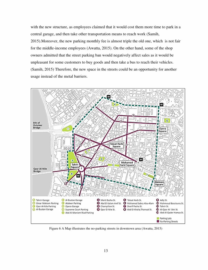
Recently in 2015, the government opened a new parking garage in Downtown with a
large capacity, and then started preventing parking throughout the Downtown area streets
for the sake of traffic ease (Awatta, 2015). The traffic police occupy the street parking
spaces with metal barriers on both sides (Samih, 2015). The authorities provide shuttle
buses to transport people from Tahrir garage to some spots in Downtown, but the service is
not sufficient and needs a lot of enhancements (Awatta, 2015). Not everyone was happy
13
with the new structure, as employees claimed that it would cost them more time to park in a
central garage, and then take other transportation means to reach work (Samih,
2015).Moreover, the new parking monthly fee is almost triple the old one, which is not fair
for the middle-income employees (Awatta, 2015). On the other hand, some of the shop
owners admitted that the street parking ban would negatively affect sales as it would be
unpleasant for some customers to buy goods and then take a bus to reach their vehicles.
(Samih, 2015) Therefore, the new space in the streets could be an opportunity for another
usage instead of the metal barriers.
Figure 6 A Map illustrates the no-parking streets in downtown area (Awatta, 2015)
14
Bicycle as an indispensable transportation mean 3.1.4
In order to design a cycling route network, all transportation systems should be
subjected to an assessment. Bicycles cannot be the only transportation mean for a certain
city, but must be integrated to the current transportation system to serve people in the best
way. This is not about which transportation mean is better than the other, but about the
most suitable transportation system for a certain area or city, In urban dense areas, bicycles
will not need much parking space and will save the time consumed waiting for public
transportation (Godefrooij & Schepel, 2010).
In general, each transportation mean has some pros and some cons, as for the bicycle,
there are many pros and limited cons. The bicycle as a transportation mean is an
environmentally friendly mean, and its usage requires simple training. Furthermore, its cost
per kilometer is low compared with other transportation means (Godefrooij & Schepel,
2010); in Egypt, a two way trip by bicycle will save around 60% of the trip’s total cost.
(Kingsley, 2014). On the other hand, the bicycle is not sufficient for long distance
travelling as it limits the size of luggage that could be taken and it has a high vulnerability
level due to the lack of respect by other road users (Godefrooij & Schepel, 2010).
Co-benefits of Cycling 3.1.5
The main aim for any transportation system is to allow access to any part of the area
served within a proper period. In that regard, the bicycle provides additional accessibility
options to its user especially in the metropolitan cities that might have narrow streets and
bad pavement conditions. Another beneficial advantage of using a bicycle is the freedom
of time, compared with public transportation means, as they have fixed times to move from
one station to another, which might not suitable for some people. The bicycle as
transportation mean is the best option for those who do not have alternatives rather than
walking, as it will increase the distances that could be reached (Deffner , Hefter , Rudolph
& Ziel, 2012).
Traffic congestion is one of the main problems in all urban areas, and the solution of
establishing new roads or extending existing ones proved its inefficiency. The bicycle could
possibly be the best solution for congestions as the road capacity will improve, and if
15
cycling routes become connected with the public transportation system that will create the
perfect mix to decrease traffic jams to the minimum (Godefrooij & Schepel, 2010).
Cycling will make cities more attractive for families in order to raise their kids in a
healthy and clean environment, as it is a people oriented way of travelling rather than being
a vehicle oriented place that limits the freedom of movements for pedestrians and increased
pollution (Godefrooij & Schepel, 2010).
CO2 is positively correlated to the distance travelled, and it is one of the most
harmful emissions to the environment. It comes mainly from motorized vehicles, where a
57% CO2 emission increment is expected between years 2005-2030 and 80% of that
increment will come from developing countries. The bicycle produces no emissions; it is an
environment friendly transportation mean and if it is promoted correctly, its usage will
potentially contribute to saving the environment and limiting the amount of pollution
(Godefrooij & Schepel, 2010).
A healthy person should have a few minutes of exercising daily; nevertheless, due to
the busy environment that urban residents live, they might forget to spend even one minute
exercising. Using the bicycle will provide a moderate time of exercise to keep in shape and
take care of one’s general body health (Ege & Krag, 2010).
As a summary, the bicycle does not need fuel, maintenance, registration, insurance,
big parking space or high acquisition cost. Its user enjoys exercising in every trip (Allen-
Munley & Daniel, 2006), It is the best alternative for all motorized means in order to save
money, energy, hustle, space and avoid noise, traffic congestions, pollution in addition to
living in a healthy way.
Factors Affecting Cycling 3.1.6
There are many factors that affect cycling in different levels. Cycling route choice by
cyclists is very relevant to the cycling route design, as they rate their satisfaction and
comfort level towards the route specifications and conditions. Some of the influential
factors are road slope, number of traffic lights, street direction, number of intersections,
street width, quality of pavement, security, traffic speed, traffic volume and number of
buses or trucks that use the street (Segadilha & da Penha Sanches, 2014).
16
Width of the street or the number of lanes is one of the major factors that affect
cycling routes design; cyclists may choose their route based on the number of lanes
(Shankwiler, 2006). The more driving lanes in the road, the more exposed cyclists are to
accidents (Segadilha & da Penha Sanches, 2014); in other words it is a safety issue for the
cyclists.
The road condition is an influential factor on cycling; it is very relevant to the service
level existing on the road, which is a safety or security issue from the cyclists’ perception.
Cyclists may avoid the use of unpaved roads (Stinson & Bhat, 2004).
Cyclists tend to use roads with low traffic volumes, and in some cases and that
decision could be influenced by the cycling experience. On the other hand, traffic volume is
not a standalone factor, as it is negatively correlated with the traffic speed on a certain road.
The higher the traffic volume, the lower the traffic speed; this factor also affects the safety
level on roads (Segadilha & da Penha Sanches, 2014). Speed and volume are an indicator
for the road functional class, the road type such as arterial, collector, and local roads
reflects the speed, volume and level of safety expected that influence the cycling flow
(Snizek , Nielsen & Skov-Petersen, 2013). 75% of accidents occur when the posted speed
limit for a certain road is higher than 35 miles per hour (Hunter , Pein & Stutts, 1996).
As a conclusion for all the main factors discussed, the safety perception is the main
factor when designing a cycling route network, as cyclists evaluate all road characteristics
and conditions including the risk of having accident or being injured (Lawson , Pakrashi ,
Ghosh & Szeto, 2013). Based on the World Health Organization report for 2013, most of
road accidents victims or injuries are cyclists, pedestrians, or motorcyclists (Asadi-Shekari ,
Moeinaddini & Zaly Shah, 2015). Safety is a highly considered factor in planning bicycle
facilities for most of the metropolitan areas (Allen-Munley & Daniel, 2006).
Previous studies about planning a Cycling network 3.1.7
Previous studies illustrate practical and applied examples in different cities that
would help in developing new practices in other areas.
3.1.7.1 Selecting Bicycle Commuting Routes Using GIS
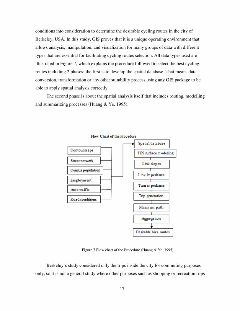
Huang, Yuanlin and Ye, Gorden (1995) introduced a study called “selecting Bicycle
Commuting Routes Using GIS” that takes travel time, volume, road slope and surface
17
conditions into consideration to determine the desirable cycling routes in the city of
Berkeley, USA. In this study, GIS proves that it is a unique operating environment that
allows analysis, manipulation, and visualization for many groups of data with different
types that are essential for facilitating cycling routes selection. All data types used are
illustrated in Figure 7, which explains the procedure followed to select the best cycling
routes including 2 phases; the first is to develop the spatial database. That means data
conversion, transformation or any other suitability process using any GIS package to be
able to apply spatial analysis correctly.
The second phase is about the spatial analysis itself that includes routing, modelling
and summarizing processes (Huang & Ye, 1995).
Figure 7 Flow chart of the Procedure (Huang & Ye, 1995)
Berkeley’s study considered only the trips inside the city for commuting purposes
only, so it is not a general study where other purposes such as shopping or recreation trips
18
are included. Inference, this study is not beneficial for people who work inside the city but
lives outside it or vice versa (Huang & Ye, 1995). Furthermore, some of the factors that
have been analyzed in this study are strongly related to the study area’s topographic nature
such as the slope; and there are other factors that might be important for this type of
analysis such as the direction of travel.
3.1.7.2 Bicycle facility planning using GIS and multi-criteria decision analysis
Many studies introduced models to plan a bicycle facility, and they are divided into
two individual groups; one of them is related to the demand based model and the other is
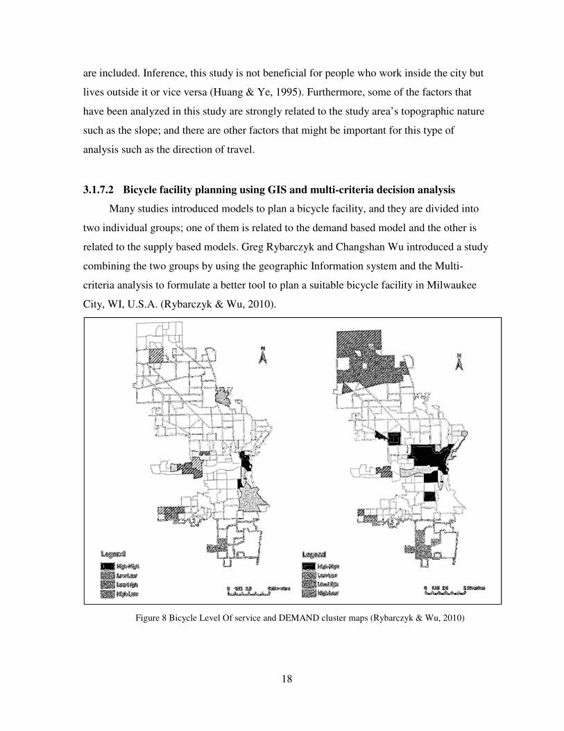
related to the supply based models. Greg Rybarczyk and Changshan Wu introduced a study
combining the two groups by using the geographic Information system and the Multi-
criteria analysis to formulate a better tool to plan a suitable bicycle facility in Milwaukee
City, WI, U.S.A. (Rybarczyk & Wu, 2010).
Figure 8 Bicycle Level Of service and DEMAND cluster maps (Rybarczyk & Wu, 2010)
19
Combining the supply and demand based models gives the planners a good
alternative method to plan a bicycle facility as the results of this study indicate that the
network analysis is able to detect the suitable road segments where the neighborhood level
analysis is a main contributor in a citywide strategic plan. That analysis, applied in terms of
Bicycle Level Of service (BLOS) grades, measures the cyclists safety based on the route
design and traffic condition versus the DEMAND on a network level and neighborhood
level (Rybarczyk & Wu, 2010).
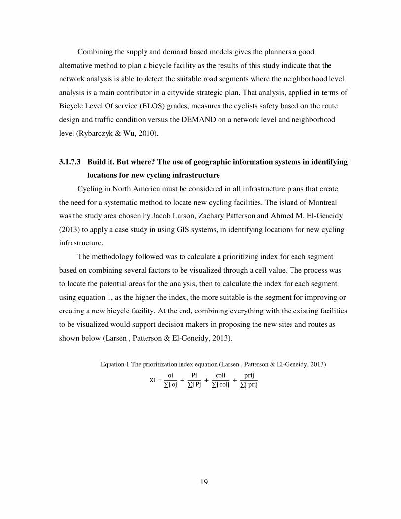
3.1.7.3 Build it. But where? The use of geographic information systems in identifying
locations for new cycling infrastructure
Cycling in North America must be considered in all infrastructure plans that create
the need for a systematic method to locate new cycling facilities. The island of Montreal
was the study area chosen by Jacob Larson, Zachary Patterson and Ahmed M. El-Geneidy
(2013) to apply a case study in using GIS systems, in identifying locations for new cycling
infrastructure.
The methodology followed was to calculate a prioritizing index for each segment
based on combining several factors to be visualized through a cell value. The process was
to locate the potential areas for the analysis, then to calculate the index for each segment
using equation 1, as the higher the index, the more suitable is the segment for improving or
creating a new bicycle facility. At the end, combining everything with the existing facilities
to be visualized would support decision makers in proposing the new sites and routes as
shown below (Larsen , Patterson & El-Geneidy, 2013).
Equation 1 The prioritization index equation (Larsen , Patterson & El-Geneidy, 2013)
Xi = oi∑joj + Pi
∑jPj + coli∑jcolj + prij
∑jprij
20
Figure 9 Display for the prioritization index applied on the Island of Montreal (Larsen , Patterson &
El-Geneidy, 2013)
This study is not presenting the ultimate method for using GIS in such a purpose,
but it illustrates the applicability to do so as the selected factors are not complete; they have
been used discreetly without any deep analysis or weighting process. GIS has been used to
analyze grid cells and various data sources such as observed bicycle trips, potential bicycle
trips, high priority segments chosen by survey respondents, bicycle accidents data, and
dead end bicycle facilities to help in planning new bicycle facilities (Larsen , Patterson &
El-Geneidy, 2013).
3.1.7.4 Urban Bicycle Route Safety Rating Model Application in Jersey City, New
Jersey
Cheryl Allen-Munley and Janice Daniels (2006) claim in their study that to increase
non-motorized transportation means usage, safety standards should take the ultimate
priority in designing routes. The main aim of this study was to develop a decision support
tool for planners to help them in establishing safe bicycle route networks in Jersey City.

21
The model used in this study is a function of nine factors including slope, traffic
volume, lane width, road classification, housing density, heavy trucks routes, direction of
travel, road condition, and daylight period. The mentioned factors were used to study and
analyze the expected severe injuries caused by bicycle-vehicle crashes or accidents (Allen-
Munley & Daniel, 2006).
Table 1 1997–2000 Jersey City Bicycle Crash Severity Index Distribution (Allen-Munley & Daniel,
2006)
NJDOT
injury
class
Injury
severity
index
Quality Description
0 1 32 Not known
1 3 0 Amputation
2 3 2 Concussion
3 3 0 Internal
4 3 36 Bleeding
5 3 59 Contusion/bruise/abrasion
6 3 0 Burn
7 3 12 Fracture/dislocation
8 2 146 Complaint of pain
9 1 27 none visible
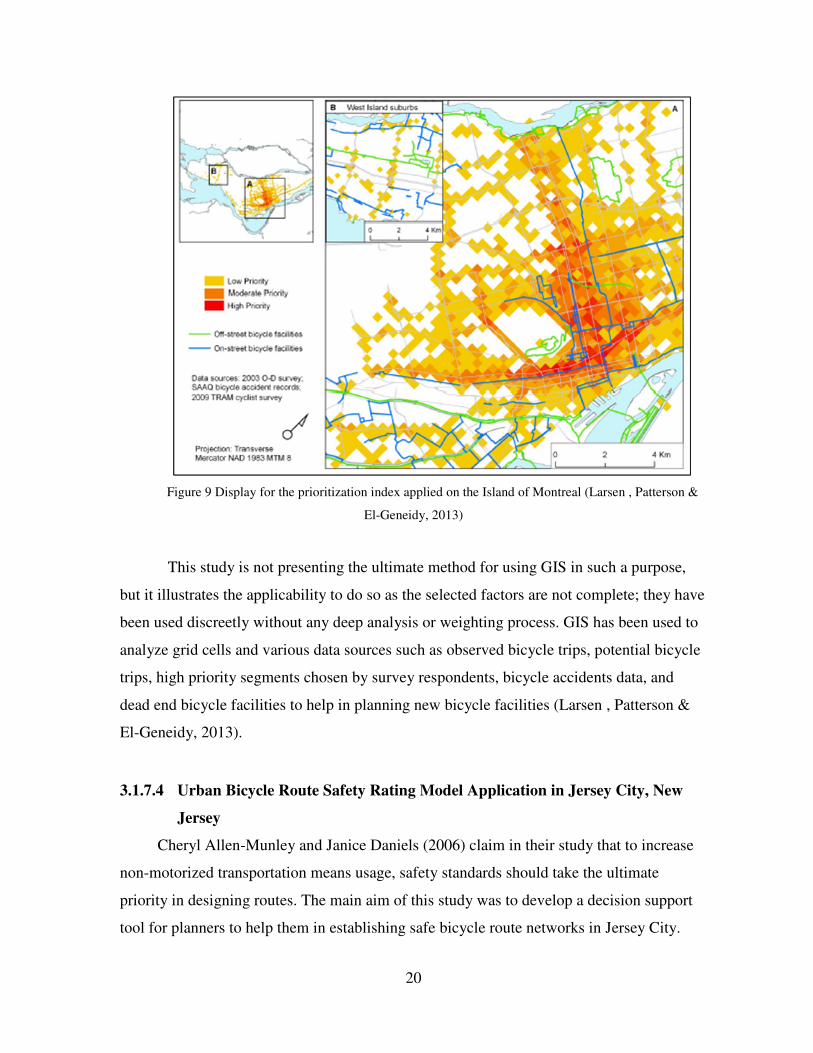
Common Methods, Theories and Models 3.1.8
There are many terminologies for bicycle facility planning, such as bicycle
suitability, bikeability, and bicycle friendliness. Bicycle friendliness is the community’s
acceptance to use the bicycle as transportation mean in their daily lives, while bikeability is
about the ease of accessibility for the intended destinations that include bicycle parking
spaces and cycling route networks’ richness. Bicycle suitability is about the level of safety
provided on the chosen or planned routes for cycling which is what this study is about
(Lowry , Callister , Gresham & Moore, 2012). Table 2 illustrates the common proposed
methods to measure bicycle suitability in terms of a score or index that assessed for a linear
segment of a bikeway using different groups of attributes.
22
Table 2 Common Bicycle Suitability Methods (Lowry , Callister , Gresham & Moore, 2012)
Name of Method Acronym Reference Reference Date
Bicycle Safety Index Rating BSIR Davis 1987
Bicycle Stress Level BSL Sorton and Walsh 1994
Road Condition Index RCI Epperson 1994
Interaction Hazard Score IHS Landis 1994
Bicycle Suitability Rating BSR Davis 1995
Bicycle Level of Service (Botma) BLOS Botma 1995
Bicycle Level of Service (Dixon) BLOS Dixon 1996
Bicycle Suitability Score BSS Turner et al 1997
Bicycle Compatibility Index BCI Harkey et al 1998
Bicycle Suitability Assessment BSA Emery and Crump 2003
Bicycle Level of Service (Jensen) BLOS Jensen 2007
Bicycle Level of Service (Petitsch et al) BLOS Petritsch et al 2007
Bicycle Level of Service (HCM) BLOS HCM 2011
In this section, some of the methods mentioned in Table 2 will be discussed briefly in
order to pick the most applicable one for the study area of Downtown.
At the very beginning, engineers and planners used to be more interested in the road
capacity, but have recently found another factor to measure called the level of service
(LOS). LOS is an indication of the road condition and the quality of using it that describes
the level of safety in terms of lane width, number of lanes, and how comfortable the road is
in terms of maneuverings and traffic jams. LOS is being measured using six grades that
start with grade A and end by grade F. Grade A indicates the perfect road for cyclists, all
factors considered, in the methodology used for the measuring, while grade F indicates the
lowest road suitability level for cycling (Epperson, 1994).
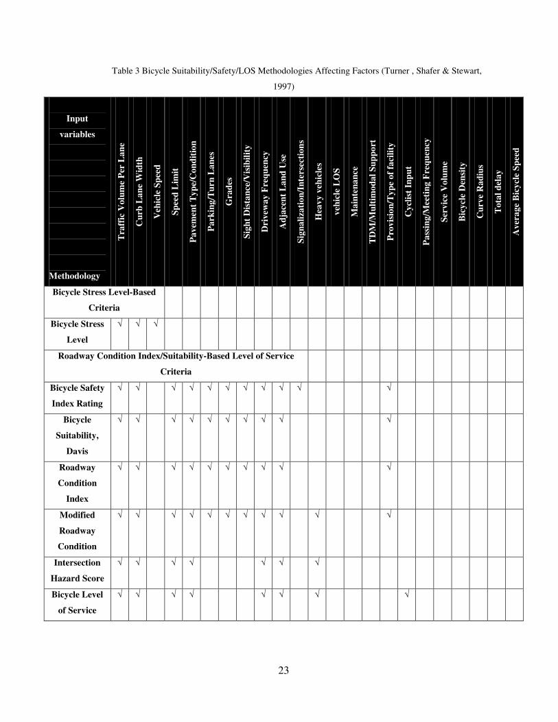
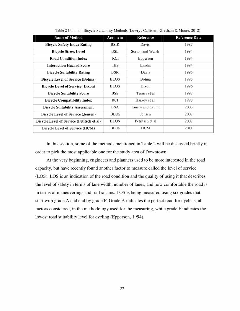
23
Table 3 Bicycle Suitability/Safety/LOS Methodologies Affecting Factors (Turner , Shafer & Stewart,
1997)
Input
variables
Methodology
Tra
ffic
Vo
lum
e P
er L
an
e
Cu
rb L
an
e W
idth
Veh
icle
Sp
eed
Sp
eed
Lim
it
Pa
vem
ent
Ty
pe/
Co
nd
itio
n
Pa
rkin
g/T
urn
La
nes
Gra
des
Sig
ht
Dis
tan
ce/V
isib
ilit
y
Dri
vew
ay
Fre
qu
ency
Ad
jace
nt
La
nd
Use
Sig
na
liza
tio
n/I
nte
rsec
tio
ns
Hea
vy
veh
icle
s
veh
icle
LO
S
Ma
inte
na
nce
TD
M/M
ult
imo
da
l S
up
po
rt
Pro
vis
ion
/Ty
pe
of
faci
lity
Cy
clis
t In
pu
t
Pa
ssin
g/M
eeti
ng
Fre
qu
ency
Ser
vic
e V
olu
me
Bic
ycl
e D
ensi
ty
Cu
rve
Ra
diu
s
To
tal
del
ay
Av
era
ge
Bic
ycl
e S
pee
d
Bicycle Stress Level-Based
Criteria
Bicycle Stress
Level
√ √ √
Roadway Condition Index/Suitability-Based Level of Service
Criteria
Bicycle Safety
Index Rating
√ √ √ √ √ √ √ √ √ √ √
Bicycle
Suitability,
Davis
√ √ √ √ √ √ √ √ √ √
Roadway
Condition
Index
√ √ √ √ √ √ √ √ √ √
Modified
Roadway
Condition
√ √ √ √ √ √ √ √ √ √ √
Intersection
Hazard Score
√ √ √ √ √ √ √
Bicycle Level
of Service
√ √ √ √ √ √ √ √
24
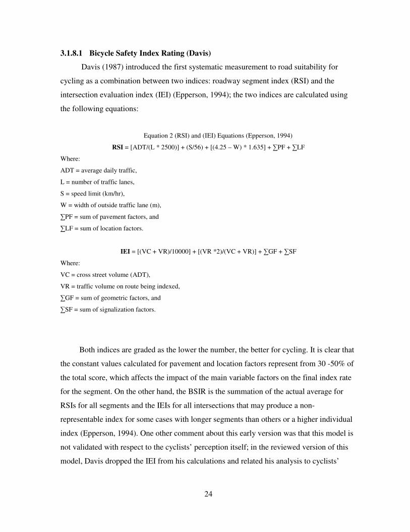
3.1.8.1 Bicycle Safety Index Rating (Davis)
Davis (1987) introduced the first systematic measurement to road suitability for
cycling as a combination between two indices: roadway segment index (RSI) and the
intersection evaluation index (IEI) (Epperson, 1994); the two indices are calculated using
the following equations:
Equation 2 (RSI) and (IEI) Equations (Epperson, 1994)
RSI = [ADT/(L * 2500)] + (S/56) + [(4.25 – W) * 1.635] + ∑PF + ∑LF
Where:
ADT = average daily traffic,
L = number of traffic lanes,
S = speed limit (km/hr),
W = width of outside traffic lane (m),
∑PF = sum of pavement factors, and
∑LF = sum of location factors.
IEI = [(VC + VR)/10000] + [(VR *2)/(VC + VR)] + ∑GF + ∑SF
Where:
VC = cross street volume (ADT),
VR = traffic volume on route being indexed,
∑GF = sum of geometric factors, and
∑SF = sum of signalization factors.
Both indices are graded as the lower the number, the better for cycling. It is clear that
the constant values calculated for pavement and location factors represent from 30 -50% of
the total score, which affects the impact of the main variable factors on the final index rate
for the segment. On the other hand, the BSIR is the summation of the actual average for
RSIs for all segments and the IEIs for all intersections that may produce a non-
representable index for some cases with longer segments than others or a higher individual
index (Epperson, 1994). One other comment about this early version was that this model is
not validated with respect to the cyclists’ perception itself; in the reviewed version of this
model, Davis dropped the IEI from his calculations and related his analysis to cyclists’
25
perception evaluation (Turner , Shafer & Stewart, 1997). In fact, Davis’ equations are the
pioneer attempt for measuring the true LOS rating for bicycles (Epperson, 1994).
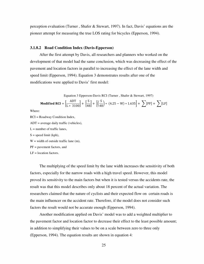
3.1.8.2 Road Condition Index (Davis-Epperson)
After the first attempt by Davis, all researchers and planners who worked on the
development of that model had the same conclusion, which was decreasing the effect of the
pavement and location factors in parallel to increasing the effect of the lane width and
speed limit (Epperson, 1994). Equation 3 demonstrates results after one of the
modifications were applied to Davis’ first model:
Equation 3 Epperson-Davis RCI (Turner , Shafer & Stewart, 1997)
����������� = � ADTL ∗ 3100 +� S
48 +�$ S48% ∗ &4.25 − W, ∗ 1.635 +./PF1 +./LF1
Where:
RCI = Roadway Condition Index,
ADT = average daily traffic (vehicles),
L = number of traffic lanes,
S = speed limit (kph),
W = width of outside traffic lane (m),
PF = pavement factors, and
LF = location factors.
The multiplying of the speed limit by the lane width increases the sensitivity of both
factors, especially for the narrow roads with a high travel speed. However, this model
proved its sensitivity to the main factors but when it is tested versus the accidents rate, the
result was that this model describes only about 18 percent of the actual variation. The
researchers claimed that the nature of cyclists and their expected flow on certain roads is
the main influencer on the accident rate. Therefore, if the model does not consider such
factors the result would not be accurate enough (Epperson, 1994).
Another modification applied on Davis’ model was to add a weighted multiplier to
the pavement factor and location factor to decrease their effect to the least possible amount;
in addition to simplifying their values to be on a scale between zero to three only
(Epperson, 1994). The equation results are shown in equation 4:
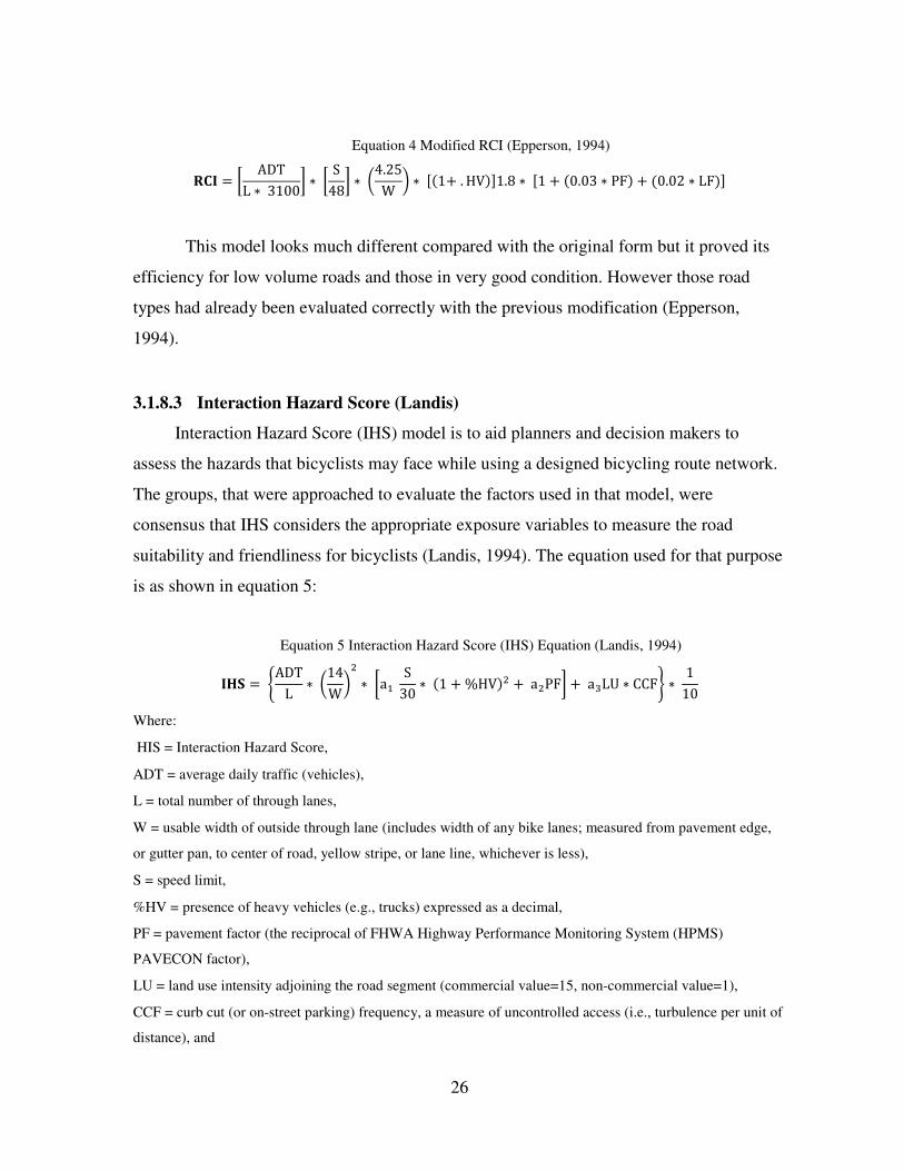
26
Equation 4 Modified RCI (Epperson, 1994)
��� = � ADTL ∗ 3100 ∗ � S
48 ∗ $4.25W % ∗ /&1+. HV,11.8 ∗ /1 + &0.03 ∗ PF, + &0.02 ∗ LF,1
This model looks much different compared with the original form but it proved its
efficiency for low volume roads and those in very good condition. However those road
types had already been evaluated correctly with the previous modification (Epperson,
1994).
3.1.8.3 Interaction Hazard Score (Landis)
Interaction Hazard Score (IHS) model is to aid planners and decision makers to
assess the hazards that bicyclists may face while using a designed bicycling route network.
The groups, that were approached to evaluate the factors used in that model, were
consensus that IHS considers the appropriate exposure variables to measure the road
suitability and friendliness for bicyclists (Landis, 1994). The equation used for that purpose
is as shown in equation 5:
Equation 5 Interaction Hazard Score (IHS) Equation (Landis, 1994)
�45 = 6ADTL ∗$14W%7 ∗ �a9 S
30 ∗ &1 + %HV,7 +a7PF +a;LU ∗ CCF> ∗ 110
Where:
HIS = Interaction Hazard Score,
ADT = average daily traffic (vehicles),
L = total number of through lanes,
W = usable width of outside through lane (includes width of any bike lanes; measured from pavement edge,
or gutter pan, to center of road, yellow stripe, or lane line, whichever is less),
S = speed limit,
%HV = presence of heavy vehicles (e.g., trucks) expressed as a decimal,
PF = pavement factor (the reciprocal of FHWA Highway Performance Monitoring System (HPMS)
PAVECON factor),
LU = land use intensity adjoining the road segment (commercial value=15, non-commercial value=1),
CCF = curb cut (or on-street parking) frequency, a measure of uncontrolled access (i.e., turbulence per unit of
distance), and
27
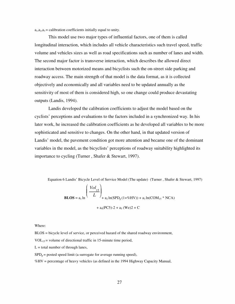
a1,a2,a3 = calibration coefficients initially equal to unity.
This model use two major types of influential factors, one of them is called
longitudinal interaction, which includes all vehicle characteristics such travel speed, traffic
volume and vehicles sizes as well as road specifications such as number of lanes and width.
The second major factor is transverse interaction, which describes the allowed direct
interaction between motorized means and bicyclists such the on-street side parking and
roadway access. The main strength of that model is the data format, as it is collected
objectively and economically and all variables need to be updated annually as the
sensitivity of most of them is considered high, so one change could produce devastating
outputs (Landis, 1994).
Landis developed the calibration coefficients to adjust the model based on the
cyclists’ perceptions and evaluations to the factors included in a synchronized way. In his
later work, he increased the calibration coefficients as he developed all variables to be more
sophisticated and sensitive to changes. On the other hand, in that updated version of
Landis’ model, the pavement condition got more attention and became one of the dominant
variables in the model, as the bicyclists’ perceptions of roadway suitability highlighted its
importance to cycling (Turner , Shafer & Stewart, 1997).
Equation 6 Landis’ Bicycle Level of Service Model (The update) (Turner , Shafer & Stewart, 1997)
BLOS = a1 ln + a2 ln(SPDp (1+%HV)) + a3 ln(COM15 * NCA)
+ a4(PC5)-2 + a5 (We)2 + C
Where:
BLOS = bicycle level of service, or perceived hazard of the shared roadway environment,
VOL15 = volume of directional traffic in 15-minute time period,
L = total number of through lanes,
SPDp = posted speed limit (a surrogate for average running speed),
%HV = percentage of heavy vehicles (as defined in the 1994 Highway Capacity Manual,
Vol 15
L
28
COM15 = trip generation intensity of the land use adjoining the road segment (stratified to a commercial trip
generation of “15,” multiplied by the percentage of the segment with adjoining commercial land development,
NCA = effective frequency per mile of non-controlled vehicular access (e.g., driveways and/or on-street
parking spaces),
PC5 = FHWA’s five point pavement surface condition rating,
We = average effective width of outside through lane:
= Wt + WI - ∑Wr
Where: Wt = total width of outside lane (and shoulder) pavement,
WI = width of paving between the outside lane stripe and the edge of pavement,
Wr = width (and frequency) of encroachments in the outside lane,
= Wp * % of segment with on-street parking + Wg
Where: Wp = width of pavement occupied by on-street parking activity,
Wg = combined width and frequency factor of other
encroachments, and,
a1 = 0.589 (calibration coefficient) a2 = 0.826 (calibration coefficient) a3 = 0.019 (calibration coefficient) a4 =
6.406 (calibration coefficient) a5 = 0.005 (calibration coefficient) C = 1.579 (calibration coefficient).
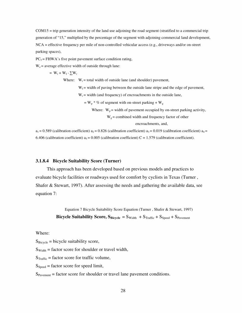
3.1.8.4 Bicycle Suitability Score (Turner)
This approach has been developed based on previous models and practices to
evaluate bicycle facilities or roadways used for comfort by cyclists in Texas (Turner ,
Shafer & Stewart, 1997). After assessing the needs and gathering the available data, see
equation 7:
Equation 7 Bicycle Suitability Score Equation (Turner , Shafer & Stewart, 1997)
Bicycle Suitability Score, SBicycle = SWidth + STraffic + SSpeed + SPavement
Where:
SBicycle = bicycle suitability score,
SWidth = factor score for shoulder or travel width,
STraffic = factor score for traffic volume,
SSpeed = factor score for speed limit,
SPavement = factor score for shoulder or travel lane pavement conditions.
29
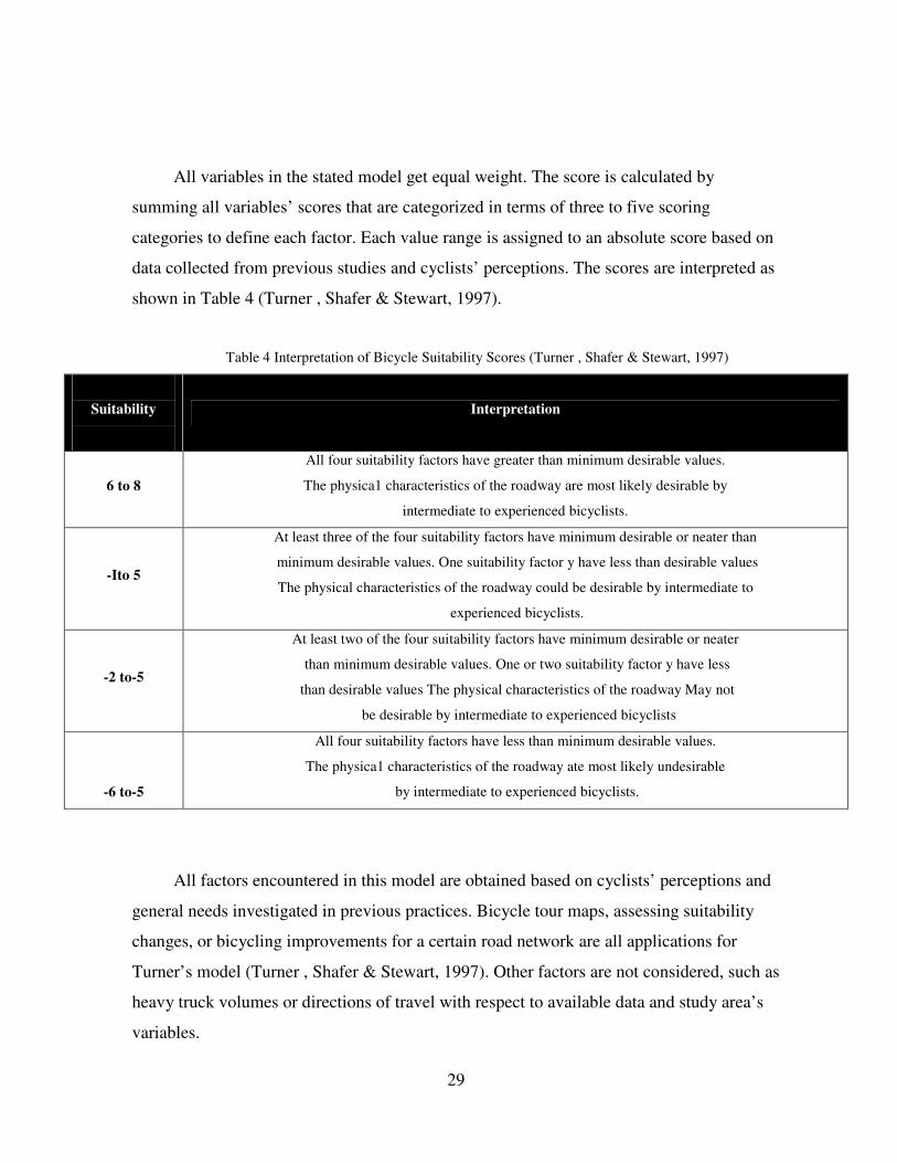
All variables in the stated model get equal weight. The score is calculated by
summing all variables’ scores that are categorized in terms of three to five scoring
categories to define each factor. Each value range is assigned to an absolute score based on
data collected from previous studies and cyclists’ perceptions. The scores are interpreted as
shown in Table 4 (Turner , Shafer & Stewart, 1997).
Table 4 Interpretation of Bicycle Suitability Scores (Turner , Shafer & Stewart, 1997)
Bicycle
Suitability
Score Range
Interpretation
6 to 8
All four suitability factors have greater than minimum desirable values.
The physica1 characteristics of the roadway are most likely desirable by
intermediate to experienced bicyclists.
-Ito 5
At least three of the four suitability factors have minimum desirable or neater than
minimum desirable values. One suitability factor y have less than desirable values
The physical characteristics of the roadway could be desirable by intermediate to
experienced bicyclists.
-2 to-5
At least two of the four suitability factors have minimum desirable or neater
than minimum desirable values. One or two suitability factor y have less
than desirable values The physical characteristics of the roadway May not
be desirable by intermediate to experienced bicyclists
-6 to-5
All four suitability factors have less than minimum desirable values.
The physica1 characteristics of the roadway ate most likely undesirable
by intermediate to experienced bicyclists.
All factors encountered in this model are obtained based on cyclists’ perceptions and
general needs investigated in previous practices. Bicycle tour maps, assessing suitability
changes, or bicycling improvements for a certain road network are all applications for
Turner’s model (Turner , Shafer & Stewart, 1997). Other factors are not considered, such as
heavy truck volumes or directions of travel with respect to available data and study area’s
variables.
30
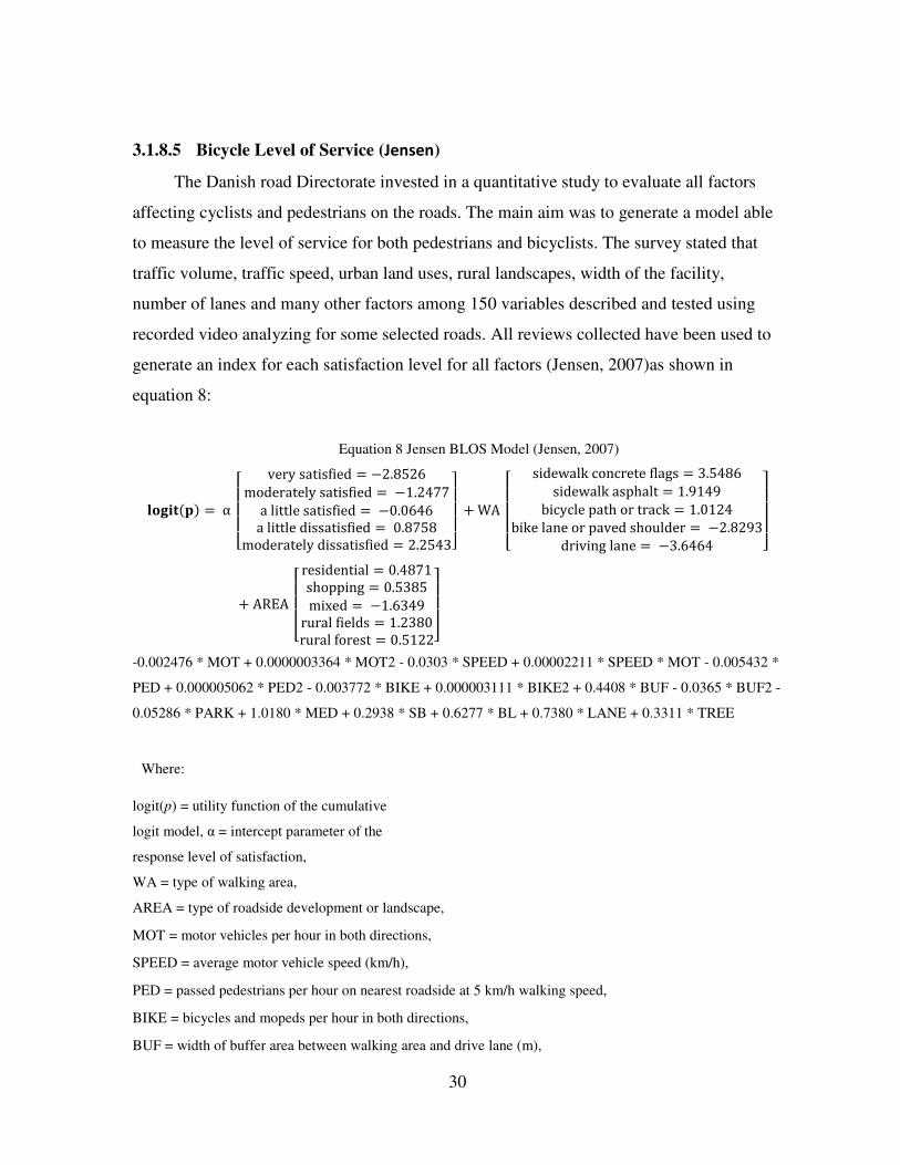
3.1.8.5 Bicycle Level of Service (Jensen)
The Danish road Directorate invested in a quantitative study to evaluate all factors
affecting cyclists and pedestrians on the roads. The main aim was to generate a model able
to measure the level of service for both pedestrians and bicyclists. The survey stated that
traffic volume, traffic speed, urban land uses, rural landscapes, width of the facility,
number of lanes and many other factors among 150 variables described and tested using
recorded video analyzing for some selected roads. All reviews collected have been used to
generate an index for each satisfaction level for all factors (Jensen, 2007)as shown in
equation 8:
Equation 8 Jensen BLOS Model (Jensen, 2007)
?�@�A&B, = αDEEEF verysatisfied = −2.8526moderatelysatisfied = −1.2477alittlesatisfied = −0.0646alittledissatisfied = 0.8758moderatelydissatisfied = 2.2543PQ
QQR+ WA
DEEEF sidewalkconcreteflags = 3.5486sidewalkasphalt = 1.9149bicyclepathortrack = 1.0124bikelaneorpavedshoulder = −2.8293drivinglane = −3.6464 PQ
QQR
+ AREADEEEF residential = 0.4871shopping = 0.5385mixed = −1.6349ruralfields = 1.2380ruralforest = 0.5122PQ
QQR
-0.002476 * MOT + 0.0000003364 * MOT2 - 0.0303 * SPEED + 0.00002211 * SPEED * MOT - 0.005432 *
PED + 0.000005062 * PED2 - 0.003772 * BIKE + 0.000003111 * BIKE2 + 0.4408 * BUF - 0.0365 * BUF2 -
0.05286 * PARK + 1.0180 * MED + 0.2938 * SB + 0.6277 * BL + 0.7380 * LANE + 0.3311 * TREE
Where:
logit(p) = utility function of the cumulative
logit model, α = intercept parameter of the
response level of satisfaction,
WA = type of walking area,
AREA = type of roadside development or landscape,
MOT = motor vehicles per hour in both directions,
SPEED = average motor vehicle speed (km/h),
PED = passed pedestrians per hour on nearest roadside at 5 km/h walking speed,
BIKE = bicycles and mopeds per hour in both directions,
BUF = width of buffer area between walking area and drive lane (m),
31
PARK = parked motor vehicle on road per 100 m,
MED = median dummy, no median = 0, median = 1,
SB = width of walking area, if this is a sidewalk or bicycle path/track (m),
BL = total width of walking area and nearest drive lane, if walking area is a bicycle lane, paved shoulder or
drive lane (m),
LANE = drive lane dummy, four or more drive lanes = 1, one to three lanes = 0, TREE = tree dummy, one
tree or more on road per 50 m = 1, otherwise 0.
This model shows the benefits for planners to design new roads, to redesign existing
roads, to improve level of service, and to put plans for long-term planning decisions
(Jensen, 2007). Many factors are taken into consideration in that model, as it was originally
made based on the Danish community’s perspective. This might lead to the need for many
enhancements and edits in order to fit the model for each study area. The degree of
importance for each factor is not the same everywhere.
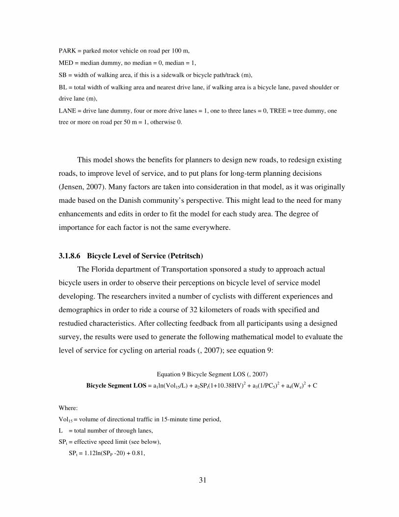
3.1.8.6 Bicycle Level of Service (Petritsch)
The Florida department of Transportation sponsored a study to approach actual
bicycle users in order to observe their perceptions on bicycle level of service model
developing. The researchers invited a number of cyclists with different experiences and
demographics in order to ride a course of 32 kilometers of roads with specified and
restudied characteristics. After collecting feedback from all participants using a designed
survey, the results were used to generate the following mathematical model to evaluate the
level of service for cycling on arterial roads (, 2007); see equation 9:
Equation 9 Bicycle Segment LOS (, 2007)
Bicycle Segment LOS = a1ln(Vol15/L) + a2SPt(1+10.38HV)2 + a3(1/PC5)2 + a4(We)
2 + C
Where:
Vol15 = volume of directional traffic in 15-minute time period,
L = total number of through lanes,
SPt = effective speed limit (see below),
SPt = 1.12ln(SPP -20) + 0.81,
32
SPP = Posted speed limit (mi/h),
HV = percentage of heavy vehicles,
PC5= FHWA’s five point surface condition rating,
We = average effective width of outside through lane,
C = a constant.
Coefficients:
a1: 0.507 a2: 0.199 a3: 7.066 a4: - 0.005 C: 0.760
Equation 10 Bicycle Facility LOS (, 2007)
Bicycle Facility LOS = a1(AvSegLOS) + a2 (NumUnsigpm) + C
Where:
AvSegLOS = distance-weighted average segment bicycle LOS along the facility,
NumUnsigpm = the number of unsignalized intersections per mile along the facility,
C = a constant.
Even though, this study included a wide cross section of cyclists, it might be not
suitable for any other kind of roads such as rural and streets with high access management
(, 2007).
3.1.8.7 Bicycle Compatibility Index (Harkey)
The main aim of Harkey’s study was to develop a new model to be used by planners
and decision makers to accommodate the streets to serve non-motorized users. Lab videos
were used to study road characteristics and list the factors affecting their compatibility.
Using the contribution of 200 volunteers in 3 different study areas, the model was created
as shown below (Harkey , Reinfurt , Knuiman , Stewart & Sorton, 1998):
Equation 11 Bicycle Compatibility Index Model (Harkey , Reinfurt , Knuiman , Stewart & Sorton,
1998)
BCI = 3.67 - 0.966BL - 0.410BLW - 0.498CLW + 0.002CLV + 0.0004OLV
+ 0.022SPD + 0.506PKG - 0.264AREA + AF
Where:
33
BL=Presence of a bicycle lane or paved shoulder >=0.9 m (no=0 , yes=1),
BLW=bicycle lane(or paved shoulder) width, m(to the nearest tenth),
CLW=curb lane width, m(to the nearest tenth),
CLV=curb lane volume, vph in one direction,
OLV=other lane(s) volume, same direction, vph,
SPD=85th percentile speed of traffic, km/h,
PKG=presence if parking lane with more than 30 percent occupancy (no=0, yes=1),
AREA=type of road side development (residential=1, other type=0),
AF=ft+fp+frt
Where:
ft=adjustment factor for truck volumes,
fp=adjustment factor for parking turnover,
frt=adjustment factor for right-turn volumes.
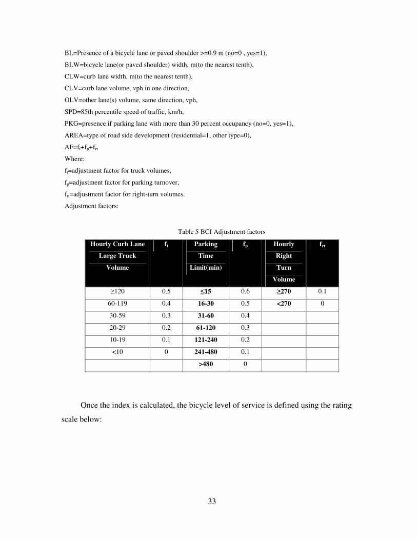
Adjustment factors:
Table 5 BCI Adjustment factors
Hourly Curb Lane
Large Truck
Volume
ft Parking
Time
Limit(min)
fp Hourly
Right
Turn
Volume
frt
≥120 0.5 ≤15 0.6 ≥270 0.1
60-119 0.4 16-30 0.5 <270 0
30-59 0.3 31-60 0.4
20-29 0.2 61-120 0.3
10-19 0.1 121-240 0.2
<10 0 241-480 0.1
>480 0
Once the index is calculated, the bicycle level of service is defined using the rating
scale below:
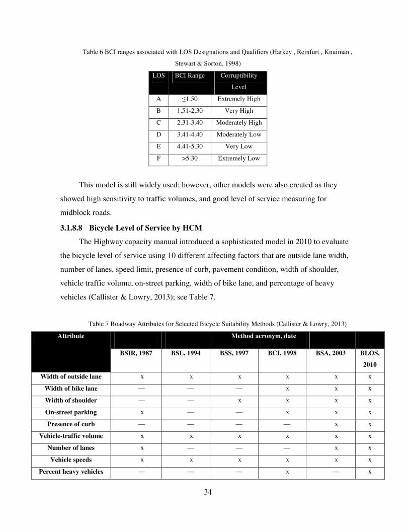
34
Table 6 BCI ranges associated with LOS Designations and Qualifiers (Harkey , Reinfurt , Knuiman ,
Stewart & Sorton, 1998)
LOS BCI Range Corruptibility
Level
A ≤1.50 Extremely High
B 1.51-2.30 Very High
C 2.31-3.40 Moderately High
D 3.41-4.40 Moderately Low
E 4.41-5.30 Very Low
F >5.30 Extremely Low
This model is still widely used; however, other models were also created as they
showed high sensitivity to traffic volumes, and good level of service measuring for
midblock roads.
3.1.8.8 Bicycle Level of Service by HCM
The Highway capacity manual introduced a sophisticated model in 2010 to evaluate
the bicycle level of service using 10 different affecting factors that are outside lane width,
number of lanes, speed limit, presence of curb, pavement condition, width of shoulder,
vehicle traffic volume, on-street parking, width of bike lane, and percentage of heavy
vehicles (Callister & Lowry, 2013); see Table 7.
Table 7 Roadway Attributes for Selected Bicycle Suitability Methods (Callister & Lowry, 2013)
Attribute Method acronym, date
BSIR, 1987 BSL, 1994 BSS, 1997 BCI, 1998 BSA, 2003 BLOS,
2010
Width of outside lane x x x x x x
Width of bike lane — — — x x x
Width of shoulder — — x x x x
On-street parking x — — x x x
Presence of curb — — — — x x
Vehicle-traffic volume x x x x x x
Number of lanes x — — — x x
Vehicle speeds x x x x x x
Percent heavy vehicles — — — x — x
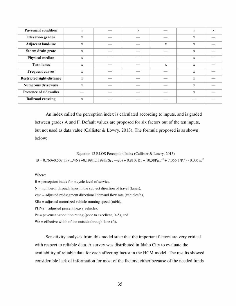
35
Pavement condition x — x — x x
Elevation grades x — — — x —
Adjacent land-use x — — x x —
Storm drain grate x — — — x —
Physical median x — — — x —
Turn lanes x — — x x —
Frequent curves x — — — x —
Restricted sight-distance x — — — x —
Numerous driveways x — — — x —
Presence of sidewalks — — — — x —
Railroad crossing x — — — — —
An index called the perception index is calculated according to inputs, and is graded
between grades A and F. Default values are proposed for six factors out of the ten inputs,
but not used as data value (Callister & Lowry, 2013). The formula proposed is as shown
below:
Equation 12 BLOS Perception Index (Callister & Lowry, 2013)
B = 0.760+0.507 ln(vma/4N) +0.199[1.1199ln(SRa —20) + 0.8103](1 + 10.38PHva)2 + 7.066(1/Pc
2) - 0.005we2
Where:
B = perception index for bicycle level of service,
N = numberof through lanes in the subject direction of travel (lanes),
vma = adjusted midsegment directional demand flow rate (vehicles/h),
SRa = adjusted motorized vehicle running speed (mi/h),
PHVa = adjusted percent heavy vehicles,
Pc = pavement-condition rating (poor to excellent, 0–5), and
We = effective width of the outside through-lane (ft).
Sensitivity analyses from this model state that the important factors are very critical
with respect to reliable data. A survey was distributed in Idaho City to evaluate the
availability of reliable data for each affecting factor in the HCM model. The results showed
considerable lack of information for most of the factors; either because of the needed funds
36
for data collection or because there was no use for such data to be collected yet (Callister &
Lowry, 2013).
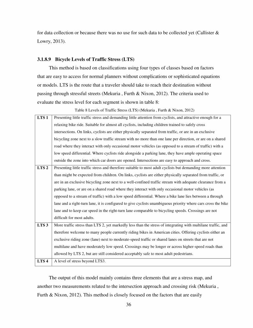
3.1.8.9 Bicycle Levels of Traffic Stress (LTS)
This method is based on classifications using four types of classes based on factors
that are easy to access for normal planners without complications or sophisticated equations
or models. LTS is the route that a traveler should take to reach their destination without
passing through stressful streets (Mekuria , Furth & Nixon, 2012). The criteria used to
evaluate the stress level for each segment is shown in table 8:
Table 8 Levels of Traffic Stress (LTS) (Mekuria , Furth & Nixon, 2012)
LTS 1 Presenting little traffic stress and demanding little attention from cyclists, and attractive enough for a
relaxing bike ride. Suitable for almost all cyclists, including children trained to safely cross
intersections. On links, cyclists are either physically separated from traffic, or are in an exclusive
bicycling zone next to a slow traffic stream with no more than one lane per direction, or are on a shared
road where they interact with only occasional motor vehicles (as opposed to a stream of traffic) with a
low speed differential. Where cyclists ride alongside a parking lane, they have ample operating space
outside the zone into which car doors are opened. Intersections are easy to approach and cross.
LTS 2 Presenting little traffic stress and therefore suitable to most adult cyclists but demanding more attention
than might be expected from children. On links, cyclists are either physically separated from traffic, or
are in an exclusive bicycling zone next to a well-confined traffic stream with adequate clearance from a
parking lane, or are on a shared road where they interact with only occasional motor vehicles (as
opposed to a stream of traffic) with a low speed differential. Where a bike lane lies between a through
lane and a right-turn lane, it is configured to give cyclists unambiguous priority where cars cross the bike
lane and to keep car speed in the right-turn lane comparable to bicycling speeds. Crossings are not
difficult for most adults.
LTS 3 More traffic stress than LTS 2, yet markedly less than the stress of integrating with multilane traffic, and
therefore welcome to many people currently riding bikes in American cities. Offering cyclists either an
exclusive riding zone (lane) next to moderate-speed traffic or shared lanes on streets that are not
multilane and have moderately low speed. Crossings may be longer or across higher-speed roads than
allowed by LTS 2, but are still considered acceptably safe to most adult pedestrians.
LTS 4 A level of stress beyond LTS3.
The output of this model mainly contains three elements that are a stress map, and
another two measurements related to the intersection approach and crossing risk (Mekuria ,
Furth & Nixon, 2012). This method is closely focused on the factors that are easily
37
controlled and based on researching, rather than those based on equations and mathematical
formulas. However, enhancements may be needed for other study areas, as the model
ignores many influencers that could strongly affect the LTS.
3.1.8.10 Which Model is the best?
Despite the fact that BLOS, which is introduced in the highway capacity manual, is
commonly used in the USA, the Bicycle compatibility index showed high sensitivity to
traffic volume and speed of travel factors (Munro, 2013). As the study area mainly suffers
from traffic jams, BCI should produce good bicycle suitability analyses for the existing
road networks. However, all models should be applied and the decision maker or the
planner would select the best fit solution.
3.2 Technical Approaches
What is GIS? 3.2.1
GIS is a set of tools used to visualize, store, analyze, capture, retrieve, question, and
interpret different types of data used to study relationships and trends in order to propose or
provide different alternatives and options for the decision makers, planners, or analysts to
select the best options for their projects (Schuurman, 2004).
GIS Applications 3.2.2
GIS has no identity, as it serves many fields and meets many interests. Some people
have an interest in “where’’, as the geographical location represents the core information
for them and GIS is a very powerful tool in dealing with such data. On the other hand,
some have an interest in ‘’how’’ or ‘’attribute data’’ as descriptive data is more important
than the location for them. GIS is very clever in sorting, analyzing, comparing, or even
dealing mathematically with numerous types of data (Schuurman, 2004).
GIS has proved its importance for many fields but in general it is powerful in finding
solutions and investigating the socio-economic and environmental problems. The core
benefit that differentiates GIS from other systems is the ability of establishing relationships
between spatial analysis and modelling or in other words linking location, condition, trend,
routing, pattern and modelling together in one output with different views (Maguire, 1991).

38
39
4 Data Required
Several sources of the data had been acquired to be analysed in order to get the best of
it. Sources were mainly govermental sectors and universities to get the most trusted data
avaialble for the study area. The missing data, that could not be sourced, has been collected
via field data collection project by the Author himself. A field sheet has been used to
collect the needed data in field.
4.1 Geometry
A shape file for all geometries in Downtown Area is required, containing all streets
with their names and a land-use coverage for the area surrounding. It could be acquired
from a private or local authority or by digitizing the area using free satellite images that is
available on the internet.
4.2 Attributes
Average Annual Daily Traffic (AADT): is the number of vehicles passing through a
certain point on a street within one year divided by 365. Vehicle/day unit expresses it
(Garber & Hoel, 2014).
Average Daily Traffic (ADT): is the number of vehicles passing through a certain point
on a street within a number greater than one day but less than one year and divided by that
number. Vehicle/day unit expresses it (Garber & Hoel, 2014).
Curb lane: is the first lane from the right hand side which is the first lane after the curb or
the pavement. (Harkey , Reinfurt & Sorton, 1998)
Curb Width: is the distance between the edge of the driving lanes and the edge of the
pavement or the sidewalk, according to the Department of Transportation of New York
City.
Direction of Travel (DOT): is the direction of driving on a certain street that might be one
way or both ways, according to wordreference.com.
Function Class (FC): is a class number represents the street’s condition or its level of
service, according to the Federal Highway Administration.
40
K-Factor: is representing a percentage of the average annual daily traffic (AADT) so it is
used to estimate or calculate the AADT or the ADT (State of Florida Department of
Transportation, 2012).
Lane Width: is the distance between the two edges’ markings that define the lane (Karim,
2015).
Number of lanes: is the number of marked passages on one street having the same
direction of travel, according to merriam-webster.com.
Pavement/Sidewalk width: is the distance between the physical edges for the space that
pedestrians can use, according to San Francisco Better Streets.
Peak Hour Volume: it is the highest number of vehicles passing through a certain point on
a street within one Hour. Vehicles/hour unit expresses it (Garber & Hoel, 2014).
Running Speed/Actual Speed/Average Speed: it is the average speed that vehicles follow
on a certain street and it is calculated by dividing the street length by the time commuted
starting from entering the street until reaching its end. Another method to calculate the
running speed is to sum a sample number of vehicles’ speeds on a certain street and divide
it by the sample size (Fitzpatrick, 2003).
Shoulder Width: is the width of the emergency stop lane that is usually existed on the
right hand side for the countries, which drive on the right and vice versa, according to the
Traffic Technology Today.
Speed Limit: is the maximum speed that a vehicle could reach on a certain street according
to its design and the law; called posted speed (Fitzpatrick, 2003).
4.3 Data Description
The average daily traffic is one of the main required variables to apply most of the
bicycle suitability models discussed in the literature review. Average daily traffic or ADT
is the average number of vehicles passing through a certain street within a period of more
than one day and less than one year. It is essential for many planning purposes such as
evaluation of the existing traffic flow or measuring the current demand, however gathering
this type of information is relatively expensive (Garber & Hoel, 2014).
The average annual daily traffic is another important variable needed for evaluating
the suitability of riding a bicycle on a certain street. Average Annual daily Traffic or
41
AADT is the average number of vehicles passing through a certain street during a period of
one full year. AADT is mainly used for the purpose of planning new highways and
designing a maintenance program (Garber & Hoel, 2014).
Counting the number of vehicles for many days or year is not the only way to get the
ADT or the AADT as the peak hour volume plays an essential role in estimating both
figures. The peak hour volume is the highest volume counted during one hour among 24
hours for the same day (World Bank, 2013). Usually the traffic counts is divided into 15
minutes periods so the highest 4 sequential quarters or intervals represent the peak hour
volume for a certain street (Anderson, 1994).
After getting, the peak hour volume then the k-factor could be used for estimating the
average daily traffic or the annual average daily traffic using the formula below:
Equation 13 Peak Hour Volume Equation (Harkey , Reinfurt , Knuiman , Stewart & Sorton, 1998)
PHV = AADT x K x D
Where:
PHV = peak-hour directional volume,
AADT = average annual daily traffic (vehicles per day),
K = peak-hour factor (the proportion of vehicles traveling during the peak hour, expressed as a decimal), and
D = directional split factor (the proportion of vehicles traveling in the peak direction during the peak hour,
expressed as a decimal).
Usually the k-factor ranges from 7% to 15% universally but as a default, it is 10% out
of the AADT for urban roads (Harkey , Reinfurt & Sorton, 1998); in other references, it
ranges from 12% to 18% out of the AADT for rural roads (Pline, 1992). What is applied for
Egypt is 10% to 12% out of the AADT for rural roads (Semeida, 2013) and (ABBAS,
2003); for urban areas k-factor ranges from 8% to 10% out of the ADT (Abd-El-Latif ,
Sabry , Yousef & Badra, 2007) while, for rural roads, the Egyptian Code of Practices states
that the peak hour ranges from 8% to 12% from the ADT.
Following the same regime for estimating the average daily traffic, universally, the
peak hour volume represents 9-10% of the ADT (Note, n.d.). On the other hand, ADT
represent 1.1% of the AADT in Egypt, approximately, according to Dr. Mostafa Sabry
(Professor of transport and traffic Engineering, Ain Shams university). For the directional
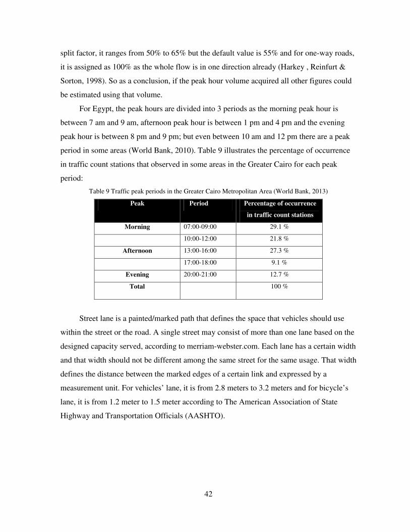
42
split factor, it ranges from 50% to 65% but the default value is 55% and for one-way roads,
it is assigned as 100% as the whole flow is in one direction already (Harkey , Reinfurt &
Sorton, 1998). So as a conclusion, if the peak hour volume acquired all other figures could
be estimated using that volume.
For Egypt, the peak hours are divided into 3 periods as the morning peak hour is
between 7 am and 9 am, afternoon peak hour is between 1 pm and 4 pm and the evening
peak hour is between 8 pm and 9 pm; but even between 10 am and 12 pm there are a peak
period in some areas (World Bank, 2010). Table 9 illustrates the percentage of occurrence
in traffic count stations that observed in some areas in the Greater Cairo for each peak
period:
Table 9 Traffic peak periods in the Greater Cairo Metropolitan Area (World Bank, 2013)
Peak Period Percentage of occurrence
in traffic count stations
Morning 07:00-09:00 29.1 %
10:00-12:00 21.8 %
Afternoon 13:00-16:00 27.3 %
17:00-18:00 9.1 %
Evening 20:00-21:00 12.7 %
Total 100 %
Street lane is a painted/marked path that defines the space that vehicles should use
within the street or the road. A single street may consist of more than one lane based on the
designed capacity served, according to merriam-webster.com. Each lane has a certain width
and that width should not be different among the same street for the same usage. That width
defines the distance between the marked edges of a certain link and expressed by a
measurement unit. For vehicles’ lane, it is from 2.8 meters to 3.2 meters and for bicycle’s
lane, it is from 1.2 meter to 1.5 meter according to The American Association of State
Highway and Transportation Officials (AASHTO).
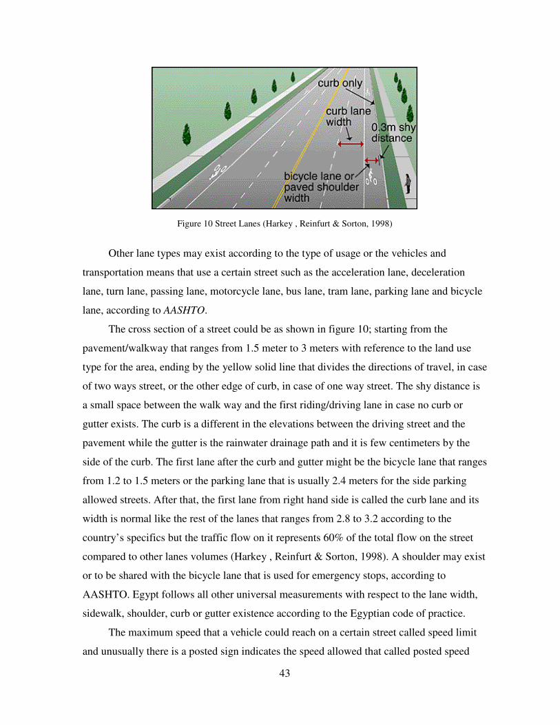
43
Figure 10 Street Lanes (Harkey , Reinfurt & Sorton, 1998)
Other lane types may exist according to the type of usage or the vehicles and
transportation means that use a certain street such as the acceleration lane, deceleration
lane, turn lane, passing lane, motorcycle lane, bus lane, tram lane, parking lane and bicycle
lane, according to AASHTO.
The cross section of a street could be as shown in figure 10; starting from the
pavement/walkway that ranges from 1.5 meter to 3 meters with reference to the land use
type for the area, ending by the yellow solid line that divides the directions of travel, in case
of two ways street, or the other edge of curb, in case of one way street. The shy distance is
a small space between the walk way and the first riding/driving lane in case no curb or
gutter exists. The curb is a different in the elevations between the driving street and the
pavement while the gutter is the rainwater drainage path and it is few centimeters by the
side of the curb. The first lane after the curb and gutter might be the bicycle lane that ranges
from 1.2 to 1.5 meters or the parking lane that is usually 2.4 meters for the side parking
allowed streets. After that, the first lane from right hand side is called the curb lane and its
width is normal like the rest of the lanes that ranges from 2.8 to 3.2 according to the
country’s specifics but the traffic flow on it represents 60% of the total flow on the street
compared to other lanes volumes (Harkey , Reinfurt & Sorton, 1998). A shoulder may exist
or to be shared with the bicycle lane that is used for emergency stops, according to
AASHTO. Egypt follows all other universal measurements with respect to the lane width,
sidewalk, shoulder, curb or gutter existence according to the Egyptian code of practice.
The maximum speed that a vehicle could reach on a certain street called speed limit
and unusually there is a posted sign indicates the speed allowed that called posted speed
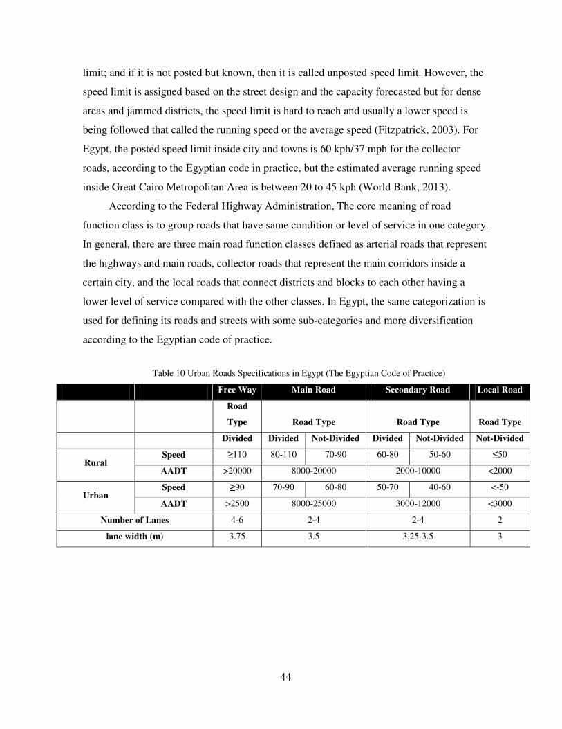
44
limit; and if it is not posted but known, then it is called unposted speed limit. However, the
speed limit is assigned based on the street design and the capacity forecasted but for dense
areas and jammed districts, the speed limit is hard to reach and usually a lower speed is
being followed that called the running speed or the average speed (Fitzpatrick, 2003). For
Egypt, the posted speed limit inside city and towns is 60 kph/37 mph for the collector
roads, according to the Egyptian code in practice, but the estimated average running speed
inside Great Cairo Metropolitan Area is between 20 to 45 kph (World Bank, 2013).
According to the Federal Highway Administration, The core meaning of road
function class is to group roads that have same condition or level of service in one category.
In general, there are three main road function classes defined as arterial roads that represent
the highways and main roads, collector roads that represent the main corridors inside a
certain city, and the local roads that connect districts and blocks to each other having a
lower level of service compared with the other classes. In Egypt, the same categorization is
used for defining its roads and streets with some sub-categories and more diversification
according to the Egyptian code of practice.
Table 10 Urban Roads Specifications in Egypt (The Egyptian Code of Practice)
Free Way Main Road Secondary Road Local Road
Road
Type Road Type Road Type Road Type
Divided Divided Not-Divided Divided Not-Divided Not-Divided
Rural Speed ≥110 80-110 70-90 60-80 50-60 ≤50
AADT >20000 8000-20000 2000-10000 <2000
Urban Speed ≥90 70-90 60-80 50-70 40-60 <-50
AADT >2500 8000-25000 3000-12000 <3000
Number of Lanes 4-6 2-4 2-4 2
lane width (m) 3.75 3.5 3.25-3.5 3
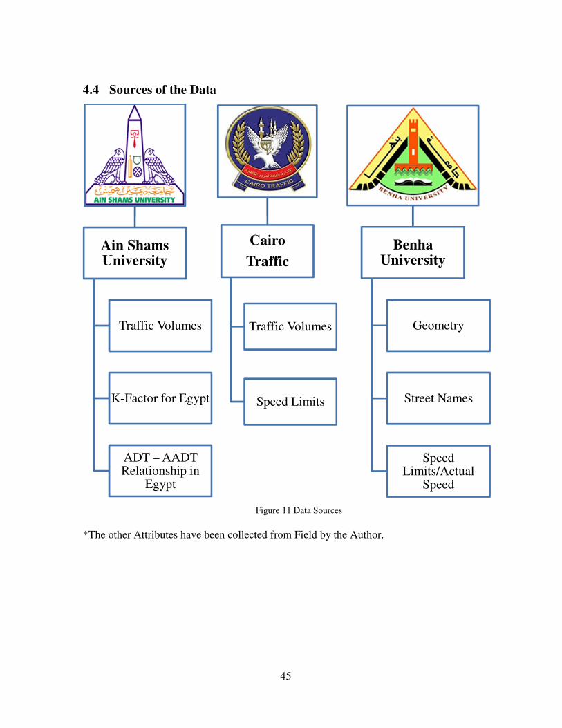
45
4.4 Sources of the Data
Figure 11 Data Sources
*The other Attributes have been collected from Field by the Author.
Ain Shams University
Traffic Volumes
K-Factor for Egypt
ADT – AADT Relationship in
Egypt
Cairo
Traffic
Traffic Volumes
Speed Limits
BenhaUniversity
Geometry
Street Names
Speed Limits/Actual
Speed
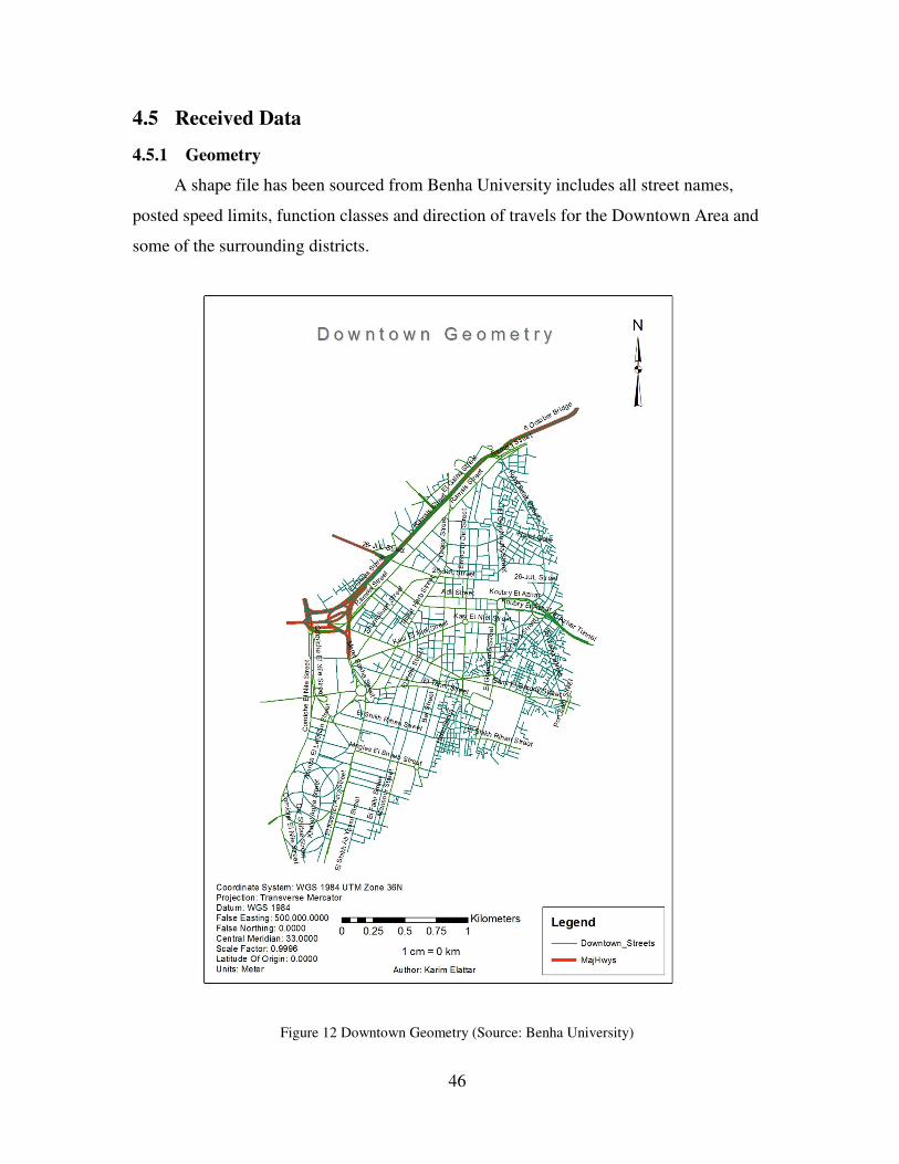
46
4.5 Received Data
Geometry 4.5.1
A shape file has been sourced from Benha University includes all street names,
posted speed limits, function classes and direction of travels for the Downtown Area and
some of the surrounding districts.
Figure 12 Downtown Geometry (Source: Benha University)
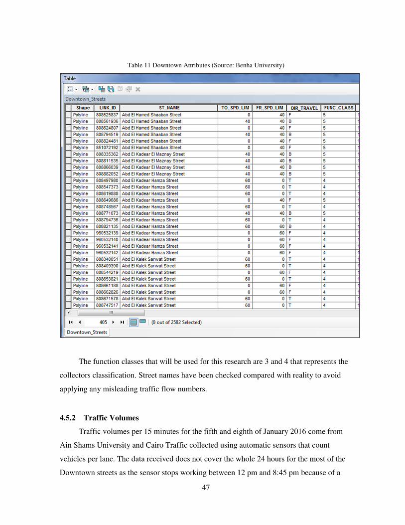
47
Table 11 Downtown Attributes (Source: Benha University)
The function classes that will be used for this research are 3 and 4 that represents the
collectors classification. Street names have been checked compared with reality to avoid
applying any misleading traffic flow numbers.
Traffic Volumes 4.5.2
Traffic volumes per 15 minutes for the fifth and eighth of January 2016 come from
Ain Shams University and Cairo Traffic collected using automatic sensors that count
vehicles per lane. The data received does not cover the whole 24 hours for the most of the
Downtown streets as the sensor stops working between 12 pm and 8:45 pm because of a
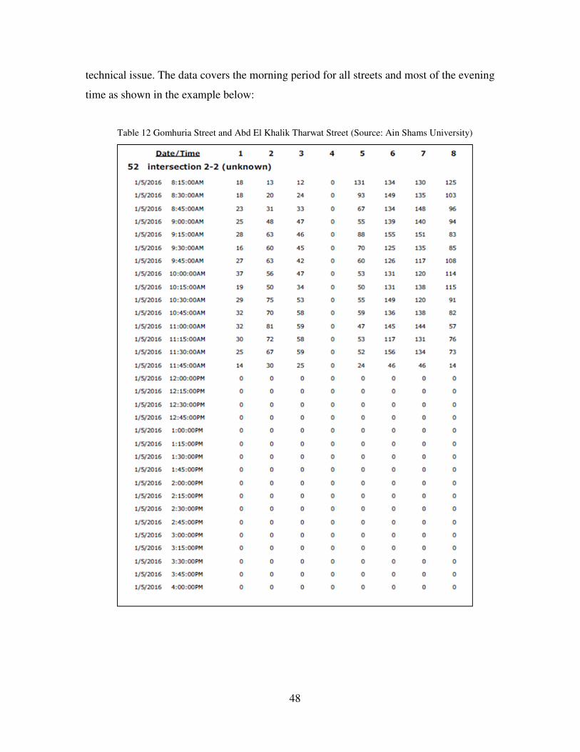
48
technical issue. The data covers the morning period for all streets and most of the evening
time as shown in the example below:
Table 12 Gomhuria Street and Abd El Khalik Tharwat Street (Source: Ain Shams University)
49
Speed Limits 4.5.3
There is no posted speed limit for the most of the Downtown streets but the default
speed limit for this admin area is 60 kph, according to the Cairo Traffic Authority. On the
other hand, the actual average speed limit for all streets in Downtown area is 40 kph,
according to Benha and Ain Shams Universities.
Street Lanes Attributes 4.5.4
The maximum number of lanes collected is four lanes and the minimum is three
lanes, according to the filed data collection. For the lane width, however the function class
is vary for the study area streets but the width of three meters per lane is measured,
according to the field data collection.

50
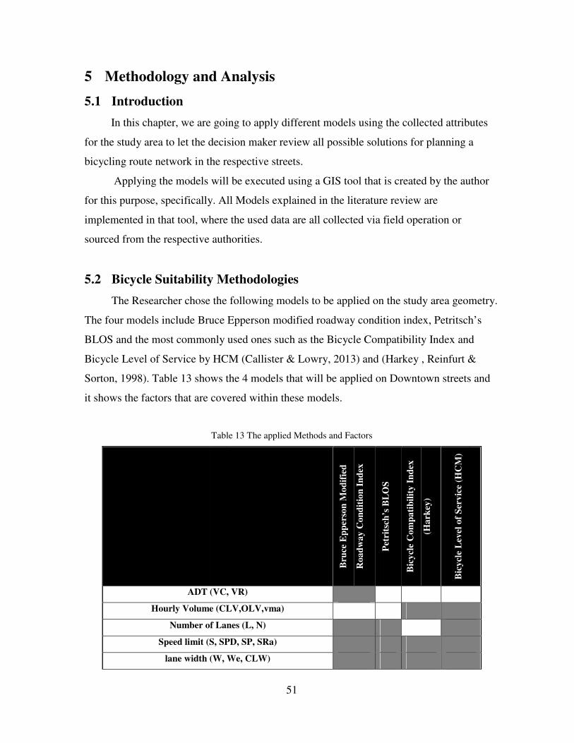
51
5 Methodology and Analysis
5.1 Introduction
In this chapter, we are going to apply different models using the collected attributes
for the study area to let the decision maker review all possible solutions for planning a
bicycling route network in the respective streets.
Applying the models will be executed using a GIS tool that is created by the author
for this purpose, specifically. All Models explained in the literature review are
implemented in that tool, where the used data are all collected via field operation or
sourced from the respective authorities.
5.2 Bicycle Suitability Methodologies
The Researcher chose the following models to be applied on the study area geometry.
The four models include Bruce Epperson modified roadway condition index, Petritsch’s
BLOS and the most commonly used ones such as the Bicycle Compatibility Index and
Bicycle Level of Service by HCM (Callister & Lowry, 2013) and (Harkey , Reinfurt &
Sorton, 1998). Table 13 shows the 4 models that will be applied on Downtown streets and
it shows the factors that are covered within these models.
Table 13 The applied Methods and Factors
Bru
ce E
pp
erso
n M
od
ifie
d
Ro
ad
wa
y C
on
dit
ion
In
dex
Pet
rits
ch’s
BL
OS
Bic
ycl
e C
om
pa
tib
ilit
y I
nd
ex
(Ha
rkey
)
Bic
ycl
e L
evel
of
Ser
vic
e (H
CM
)
ADT (VC, VR)
Hourly Volume (CLV,OLV,vma)
Number of Lanes (L, N)
Speed limit (S, SPD, SP, SRa)
lane width (W, We, CLW)
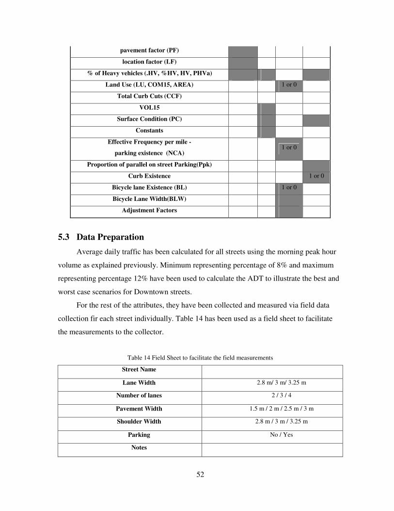
52
pavement factor (PF)
location factor (LF)
% of Heavy vehicles (.HV, %HV, HV, PHVa)
Land Use (LU, COM15, AREA) 1 or 0
Total Curb Cuts (CCF)
VOL15
Surface Condition (PC)
Constants
Effective Frequency per mile -
parking existence (NCA) 1 or 0
Proportion of parallel on street Parking(Ppk)
Curb Existence 1 or 0
Bicycle lane Existence (BL) 1 or 0
Bicycle Lane Width(BLW)
Adjustment Factors
5.3 Data Preparation
Average daily traffic has been calculated for all streets using the morning peak hour
volume as explained previously. Minimum representing percentage of 8% and maximum
representing percentage 12% have been used to calculate the ADT to illustrate the best and
worst case scenarios for Downtown streets.
For the rest of the attributes, they have been collected and measured via field data
collection fir each street individually. Table 14 has been used as a field sheet to facilitate
the measurements to the collector.
Table 14 Field Sheet to facilitate the field measurements
Street Name
Lane Width 2.8 m/ 3 m/ 3.25 m
Number of lanes 2 / 3 / 4
Pavement Width 1.5 m / 2 m / 2.5 m / 3 m
Shoulder Width 2.8 m / 3 m / 3.25 m
Parking No / Yes
Notes
53
Microsoft Excel has been used to spread all calculations for all needed attributes
and to spread the collected ones as well. Then all attributes have been copied to the
attribute table in the ArcMap.
5.4 The Bicycle Suitability Modelling Tool
A GIS tool has been developed to aid in applying all bicycling suitability models on
any geometry needed. The tool contains the majority of the suitability models excluding
any points based models such as the Bicycle Stress level and the Bicycle Levels of Traffic
Stress. All other models are included in this tool such as Davis Bicycle Safety Index
Rating, Epperson- Davis Roadway Condition Index, Bruce Epperson Modified Roadway
Condition Index, Intersection Hazard Score - BRUCE W. LANDIS, Landis’ BLOS,
Petritsch’s BLOS, Bicycle Compatibility Index (Harkey) and Bicycle Level of Service
(HCM).
Microsoft Visual studio has been used to develop the Bicycle Suitability Modelling
tool. Microsoft Visual Studio consists of multiple development platforms in order to form
one integrated development environment. It is developed by Microsoft to be used for
creating computer programs, web sites, web applications and web services supporting
multiple programming languages such as C, C++, VB.NET and many others (Johnson,
2012). The programming language used in VB.NET to create the Bicycle Suitability
Modelling Tool using the ESRI libraries that are impeded in ArcObject 10 and the compiler
is .NET Frame Work 3.5. This tool is applicable with ArcMap versions of 10 and 10.2.
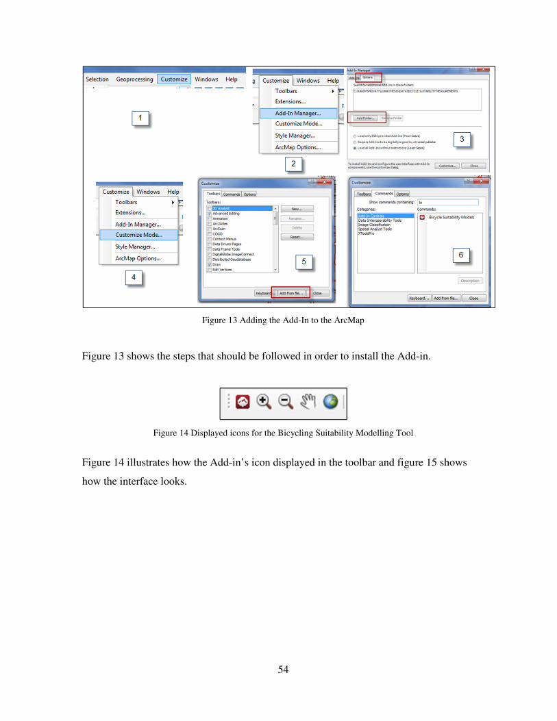
54
Figure 13 Adding the Add-In to the ArcMap
Figure 13 shows the steps that should be followed in order to install the Add-in.
Figure 14 Displayed icons for the Bicycling Suitability Modelling Tool
Figure 14 illustrates how the Add-in’s icon displayed in the toolbar and figure 15 shows
how the interface looks.
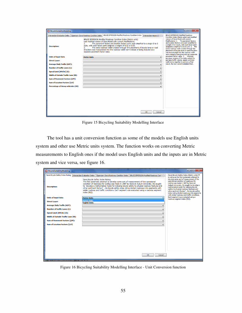
55
Figure 15 Bicycling Suitability Modelling Interface
The tool has a unit conversion function as some of the models use English units
system and other use Metric units system. The function works on converting Metric
measurements to English ones if the model uses English units and the inputs are in Metric
system and vice versa, see figure 16.
Figure 16 Bicycling Suitability Modelling Interface - Unit Conversion function
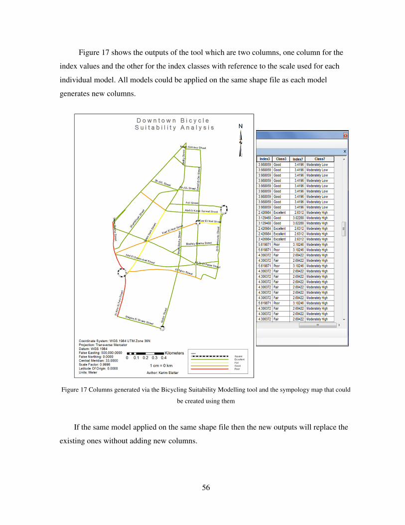
56
Figure 17 shows the outputs of the tool which are two columns, one column for the
index values and the other for the index classes with reference to the scale used for each
individual model. All models could be applied on the same shape file as each model
generates new columns.
Figure 17 Columns generated via the Bicycling Suitability Modelling tool and the sympology map that could
be created using them
If the same model applied on the same shape file then the new outputs will replace the
existing ones without adding new columns.
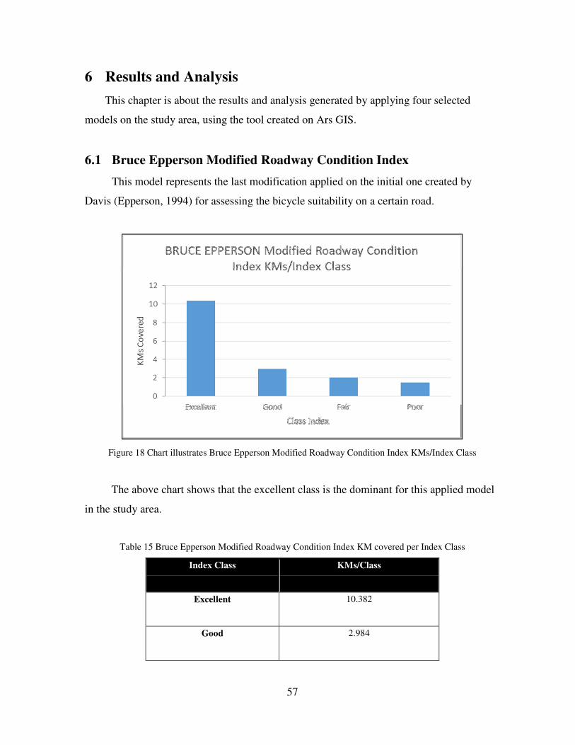
57
6 Results and Analysis
This chapter is about the results and analysis generated by applying four selected
models on the study area, using the tool created on Ars GIS.
6.1 Bruce Epperson Modified Roadway Condition Index
This model represents the last modification applied on the initial one created by
Davis (Epperson, 1994) for assessing the bicycle suitability on a certain road.
Figure 18 Chart illustrates Bruce Epperson Modified Roadway Condition Index KMs/Index Class
The above chart shows that the excellent class is the dominant for this applied model
in the study area.
Table 15 Bruce Epperson Modified Roadway Condition Index KM covered per Index Class
Index Class
KMs/Class
Excellent
10.382
Good
2.984
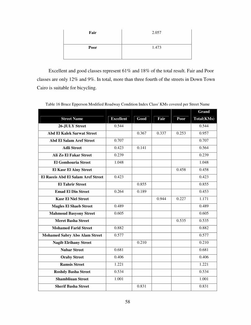
58
Fair
2.057
Poor
1.473
Excellent and good classes represent 61% and 18% of the total result. Fair and Poor
classes are only 12% and 9%. In total, more than three fourth of the streets in Down Town
Cairo is suitable for bicycling.
Table 16 Bruce Epperson Modified Roadway Condition Index Class' KMs covered per Street Name
Street Name Excellent Good Fair Poor
Grand
Total(KMs)
26-JULY Street 0.544 0.544
Abd El Kalek Sarwat Street 0.367 0.337 0.253 0.957
Abd El Salam Aref Street 0.707 0.707
Adli Street 0.423 0.141 0.564
Ali Zo El Fakar Street 0.239 0.239
El Gomhouria Street 1.048 1.048
El Kasr El Ainy Street 0.458 0.458
El Raeeis Abd El Salam Aref Street 0.423 0.423
El Tahrir Street 0.855 0.855
Emad El Din Street 0.264 0.189 0.453
Kasr El Niel Street 0.944 0.227 1.171
Magles El Shaeb Street 0.489 0.489
Mahmoud Basyony Street 0.605 0.605
Meret Basha Street 0.535 0.535
Mohamed Farid Street 0.882 0.882
Mohamed Sabry Abo Alam Street 0.577 0.577
Nagib Elrihany Street 0.210 0.210
Nubar Street 0.681 0.681
Oraby Street 0.406 0.406
Ramsis Street 1.221 1.221
Roshdy Basha Street 0.534 0.534
Shambliuan Street 1.001 1.001
Sherif Basha Street 0.831 0.831
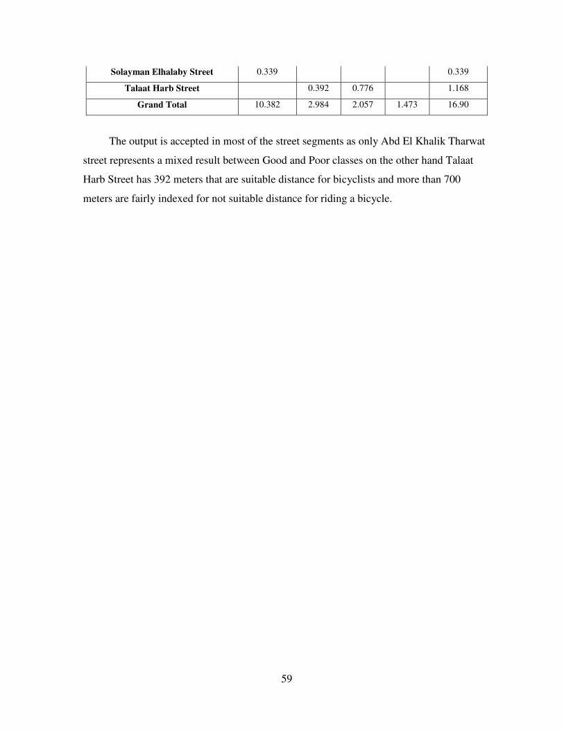
59
Solayman Elhalaby Street 0.339 0.339
Talaat Harb Street 0.392 0.776 1.168
Grand Total 10.382 2.984 2.057 1.473 16.90
The output is accepted in most of the street segments as only Abd El Khalik Tharwat
street represents a mixed result between Good and Poor classes on the other hand Talaat
Harb Street has 392 meters that are suitable distance for bicyclists and more than 700
meters are fairly indexed for not suitable distance for riding a bicycle.
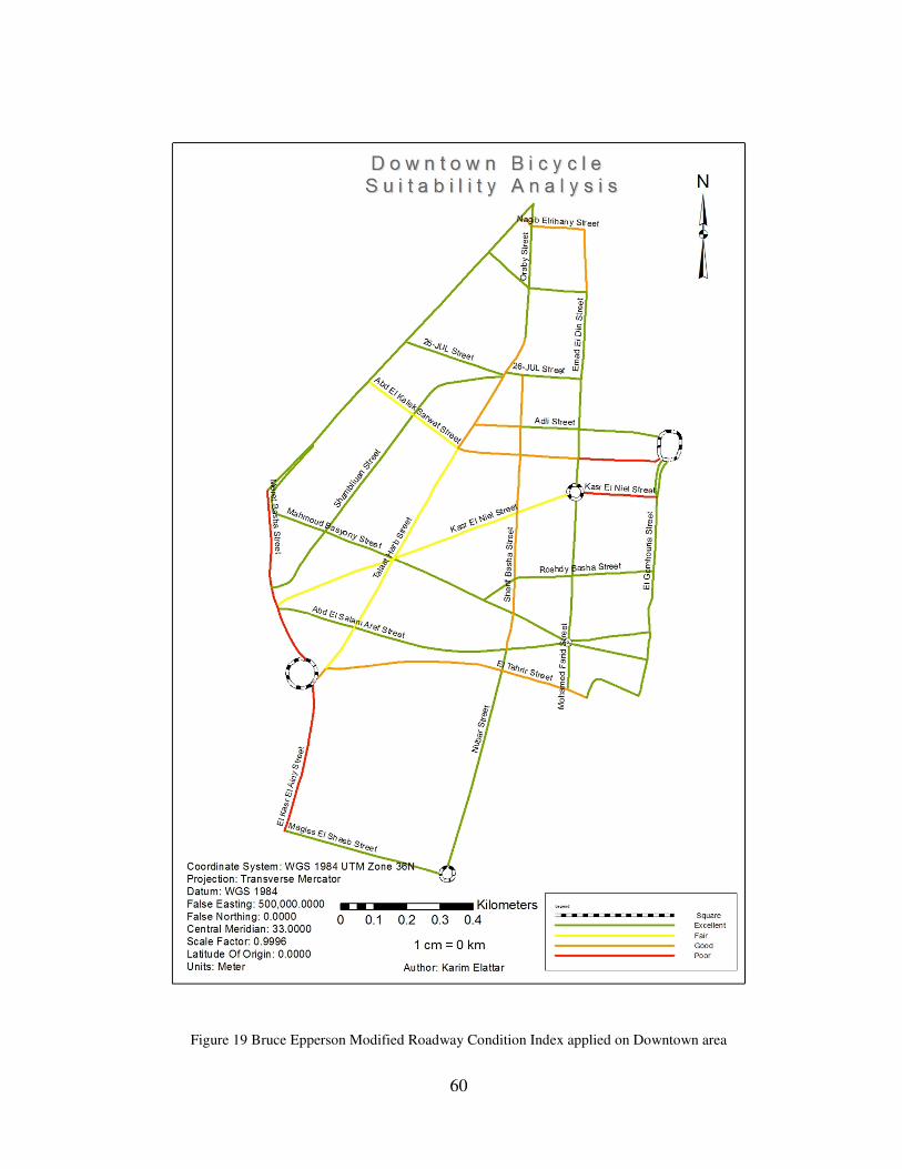
60
Figure 19 Bruce Epperson Modified Roadway Condition Index applied on Downtown area
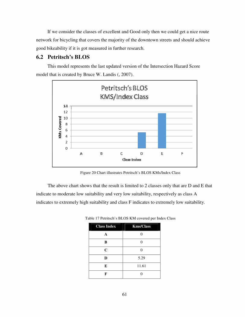
61
If we consider the classes of excellent and Good only then we could get a nice route
network for bicycling that covers the majority of the downtown streets and should achieve
good bikeability if it is got measured in further research.
6.2 Petritsch’s BLOS
This model represents the last updated version of the Intersection Hazard Score
model that is created by Bruce W. Landis (, 2007).
Figure 20 Chart illustrates Petritsch’s BLOS KMs/Index Class
The above chart shows that the result is limited to 2 classes only that are D and E that
indicate to moderate low suitability and very low suitability, respectively as class A
indicates to extremely high suitability and class F indicates to extremely low suitability.
Table 17 Petritsch’s BLOS KM covered per Index Class
Class Index Kms/Class
A 0
B 0
C 0
D 5.29
E 11.61
F 0
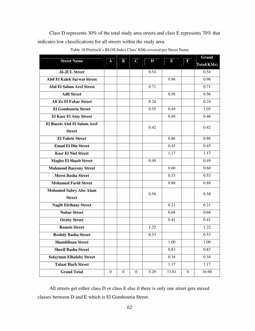
62
Class D represents 30% of the total study area streets and class E represents 70% that
indicates low classifications for all streets within the study area.
Table 18 Petritsch’s BLOS Index Class' KMs covered per Street Name
Street Name A B C D E F Grand
Total(KMs)
26-JUL Street 0.54 0.54
Abd El Kalek Sarwat Street 0.96 0.96
Abd El Salam Aref Street 0.71 0.71
Adli Street 0.56 0.56
Ali Zo El Fakar Street 0.24 0.24
El Gomhouria Street 0.55 0.49 1.05
El Kasr El Ainy Street 0.46 0.46
El Raeeis Abd El Salam Aref
Street 0.42 0.42
El Tahrir Street 0.86 0.86
Emad El Din Street 0.45 0.45
Kasr El Niel Street 1.17 1.17
Magles El Shaeb Street 0.49 0.49
Mahmoud Basyony Street 0.60 0.60
Meret Basha Street 0.53 0.53
Mohamed Farid Street 0.88 0.88
Mohamed Sabry Abo Alam
Street 0.58 0.58
Nagib Elrihany Street 0.21 0.21
Nubar Street 0.68 0.68
Oraby Street 0.41 0.41
Ramsis Street 1.22 1.22
Roshdy Basha Street 0.53 0.53
Shambliuan Street 1.00 1.00
Sherif Basha Street 0.83 0.83
Solayman Elhalaby Street 0.34 0.34
Talaat Harb Street 1.17 1.17
Grand Total 0 0 0 5.29 11.61 0 16.90
All streets get either class D or class E else if there is only one street gets mixed
classes between D and E which is El Gomhouria Street.
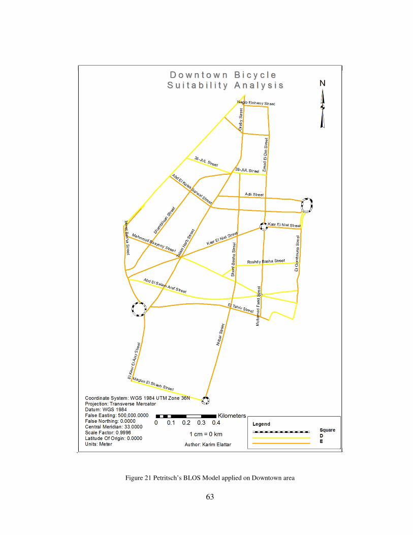
63
Figure 21 Petritsch’s BLOS Model applied on Downtown area
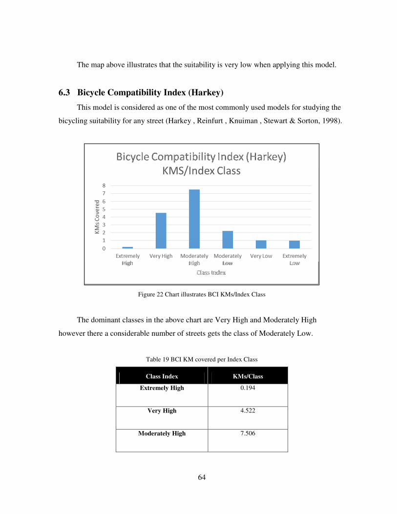
64
The map above illustrates that the suitability is very low when applying this model.
6.3 Bicycle Compatibility Index (Harkey)
This model is considered as one of the most commonly used models for studying the
bicycling suitability for any street (Harkey , Reinfurt , Knuiman , Stewart & Sorton, 1998).
Figure 22 Chart illustrates BCI KMs/Index Class
The dominant classes in the above chart are Very High and Moderately High
however there a considerable number of streets gets the class of Moderately Low.
Table 19 BCI KM covered per Index Class
Class Index KMs/Class
Extremely High
0.194
Very High
4.522
Moderately High
7.506
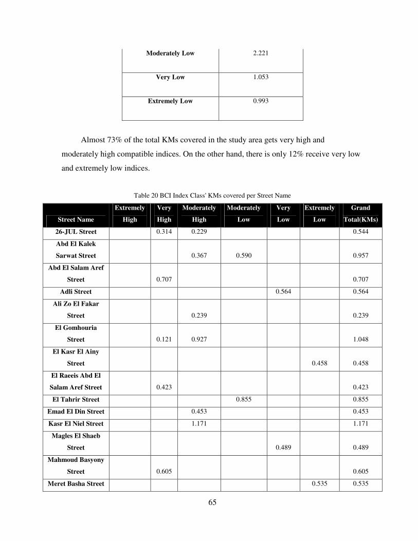
65
Moderately Low
2.221
Very Low
1.053
Extremely Low
0.993
Almost 73% of the total KMs covered in the study area gets very high and
moderately high compatible indices. On the other hand, there is only 12% receive very low
and extremely low indices.
Table 20 BCI Index Class' KMs covered per Street Name
Street Name
Extremely
High
Very
High
Moderately
High
Moderately
Low
Very
Low
Extremely
Low
Grand
Total(KMs)
26-JUL Street 0.314 0.229 0.544
Abd El Kalek
Sarwat Street 0.367 0.590 0.957
Abd El Salam Aref
Street 0.707 0.707
Adli Street 0.564 0.564
Ali Zo El Fakar
Street 0.239 0.239
El Gomhouria
Street 0.121 0.927 1.048
El Kasr El Ainy
Street 0.458 0.458
El Raeeis Abd El
Salam Aref Street 0.423 0.423
El Tahrir Street 0.855 0.855
Emad El Din Street 0.453 0.453
Kasr El Niel Street 1.171 1.171
Magles El Shaeb
Street 0.489 0.489
Mahmoud Basyony
Street 0.605 0.605
Meret Basha Street 0.535 0.535
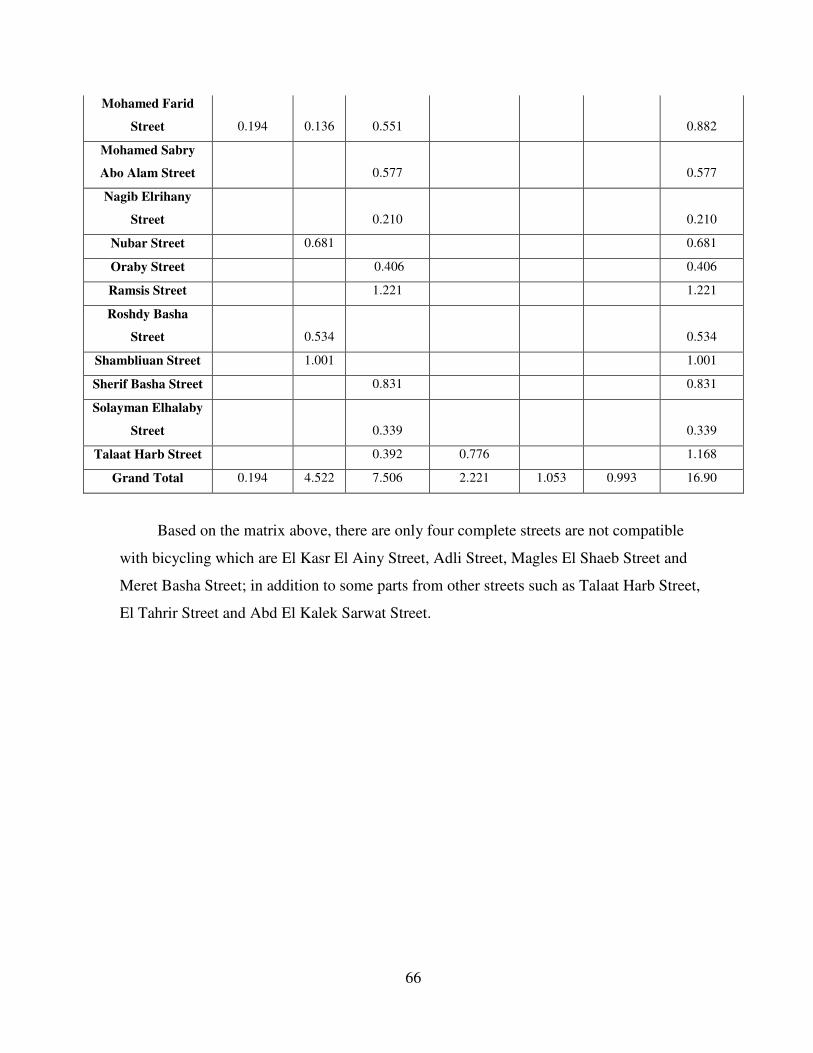
66
Mohamed Farid
Street 0.194 0.136 0.551 0.882
Mohamed Sabry
Abo Alam Street 0.577 0.577
Nagib Elrihany
Street 0.210 0.210
Nubar Street 0.681 0.681
Oraby Street 0.406 0.406
Ramsis Street 1.221 1.221
Roshdy Basha
Street 0.534 0.534
Shambliuan Street 1.001 1.001
Sherif Basha Street 0.831 0.831
Solayman Elhalaby
Street 0.339 0.339
Talaat Harb Street 0.392 0.776 1.168
Grand Total 0.194 4.522 7.506 2.221 1.053 0.993 16.90
Based on the matrix above, there are only four complete streets are not compatible
with bicycling which are El Kasr El Ainy Street, Adli Street, Magles El Shaeb Street and
Meret Basha Street; in addition to some parts from other streets such as Talaat Harb Street,
El Tahrir Street and Abd El Kalek Sarwat Street.
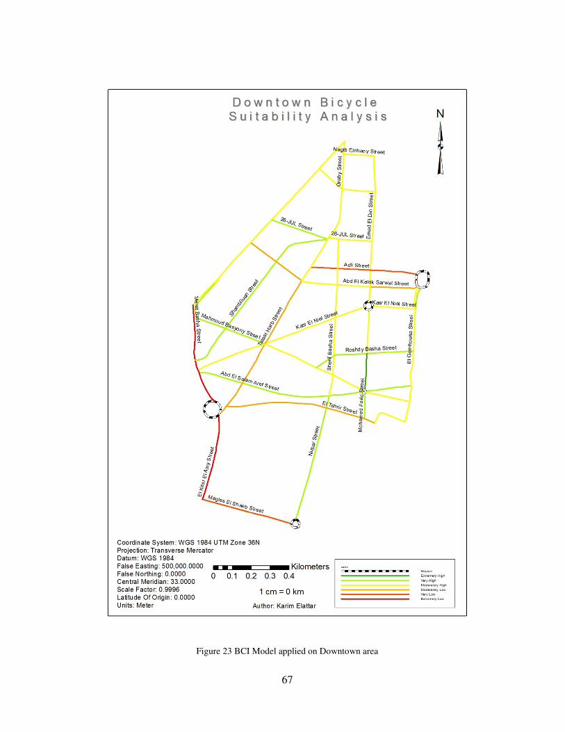
67
Figure 23 BCI Model applied on Downtown area
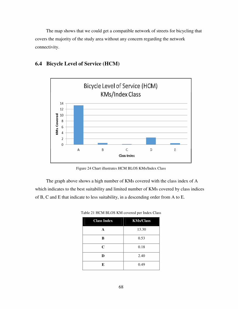
68
The map shows that we could get a compatible network of streets for bicycling that
covers the majority of the study area without any concern regarding the network
connectivity.
6.4 Bicycle Level of Service (HCM)
Figure 24 Chart illustrates HCM BLOS KMs/Index Class
The graph above shows a high number of KMs covered with the class index of A
which indicates to the best suitability and limited number of KMs covered by class indices
of B, C and E that indicate to less suitability, in a descending order from A to E.
Table 21 HCM BLOS KM covered per Index Class
Class Index KMs/Class
A 13.30
B 0.53
C 0.18
D 2.40
E 0.49
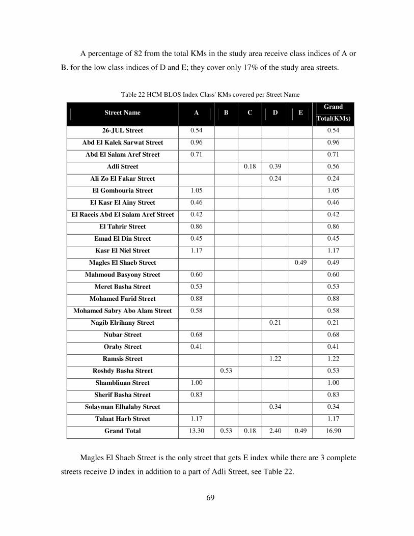
69
A percentage of 82 from the total KMs in the study area receive class indices of A or
B. for the low class indices of D and E; they cover only 17% of the study area streets.
Table 22 HCM BLOS Index Class' KMs covered per Street Name
Street Name A B C D E Grand
Total(KMs)
26-JUL Street 0.54 0.54
Abd El Kalek Sarwat Street 0.96 0.96
Abd El Salam Aref Street 0.71 0.71
Adli Street 0.18 0.39 0.56
Ali Zo El Fakar Street 0.24 0.24
El Gomhouria Street 1.05 1.05
El Kasr El Ainy Street 0.46 0.46
El Raeeis Abd El Salam Aref Street 0.42 0.42
El Tahrir Street 0.86 0.86
Emad El Din Street 0.45 0.45
Kasr El Niel Street 1.17 1.17
Magles El Shaeb Street 0.49 0.49
Mahmoud Basyony Street 0.60 0.60
Meret Basha Street 0.53 0.53
Mohamed Farid Street 0.88 0.88
Mohamed Sabry Abo Alam Street 0.58 0.58
Nagib Elrihany Street 0.21
0.21
Nubar Street 0.68 0.68
Oraby Street 0.41 0.41
Ramsis Street 1.22 1.22
Roshdy Basha Street 0.53 0.53
Shambliuan Street 1.00 1.00
Sherif Basha Street 0.83 0.83
Solayman Elhalaby Street 0.34 0.34
Talaat Harb Street 1.17 1.17
Grand Total 13.30 0.53 0.18 2.40 0.49 16.90
Magles El Shaeb Street is the only street that gets E index while there are 3 complete
streets receive D index in addition to a part of Adli Street, see Table 22.
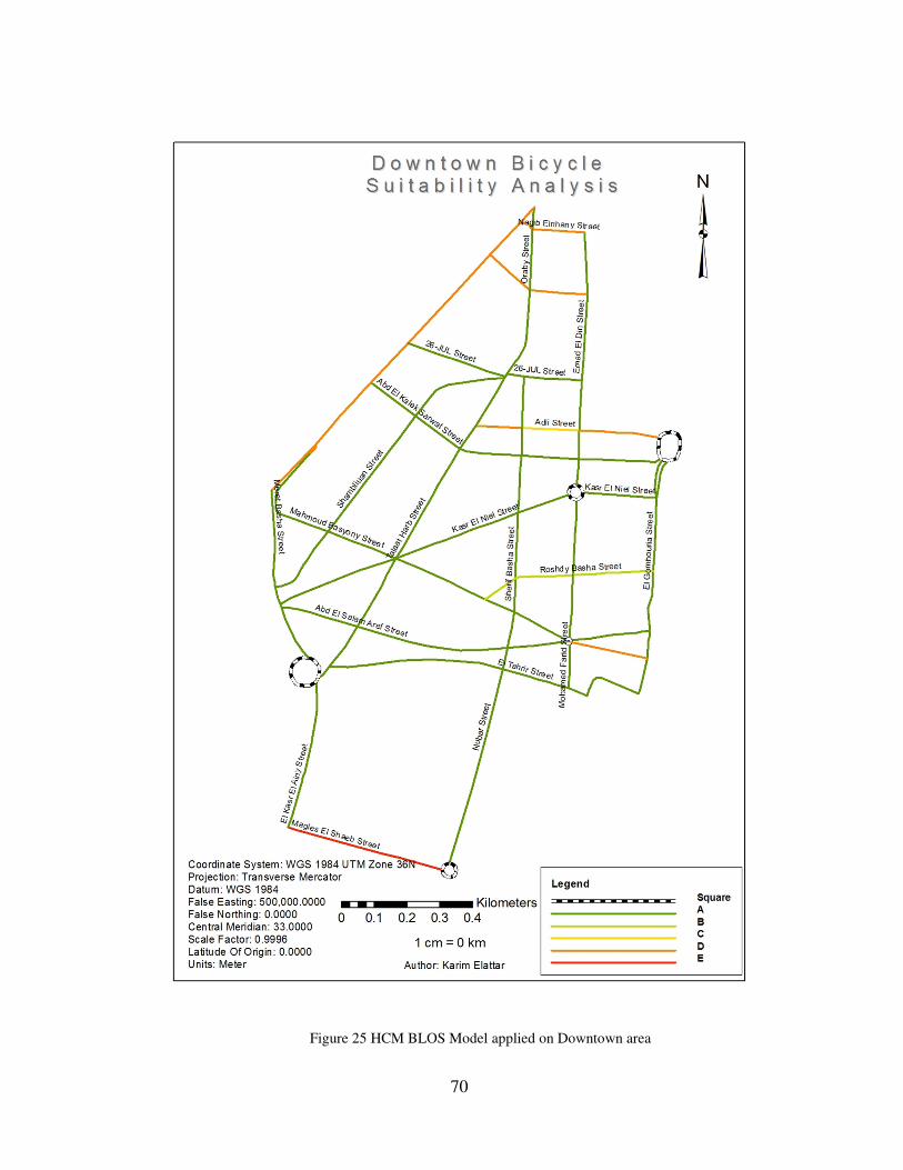
70
Figure 25 HCM BLOS Model applied on Downtown area
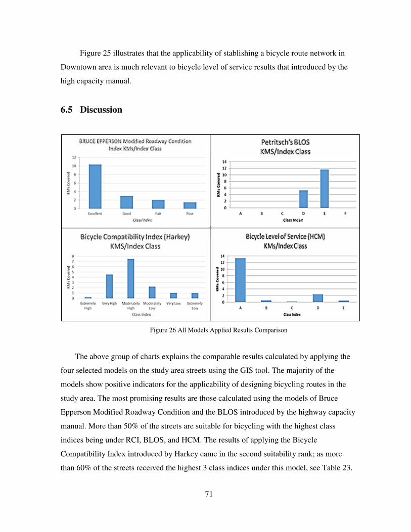
71
Figure 25 illustrates that the applicability of stablishing a bicycle route network in
Downtown area is much relevant to bicycle level of service results that introduced by the
high capacity manual.
6.5 Discussion
Figure 26 All Models Applied Results Comparison
The above group of charts explains the comparable results calculated by applying the
four selected models on the study area streets using the GIS tool. The majority of the
models show positive indicators for the applicability of designing bicycling routes in the
study area. The most promising results are those calculated using the models of Bruce
Epperson Modified Roadway Condition and the BLOS introduced by the highway capacity
manual. More than 50% of the streets are suitable for bicycling with the highest class
indices being under RCI, BLOS, and HCM. The results of applying the Bicycle
Compatibility Index introduced by Harkey came in the second suitability rank; as more
than 60% of the streets received the highest 3 class indices under this model, see Table 23.
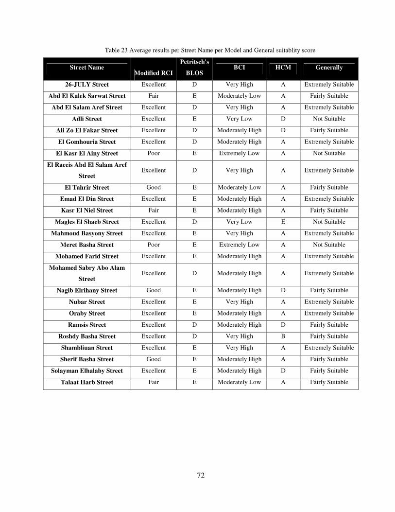
72
Table 23 Average results per Street Name per Model and General suitablity score
Street Name Modified RCI
Petritsch's
BLOS BCI HCM Generally
26-JULY Street Excellent D Very High A Extremely Suitable
Abd El Kalek Sarwat Street Fair E Moderately Low A Fairly Suitable
Abd El Salam Aref Street Excellent D Very High A Extremely Suitable
Adli Street Excellent E Very Low D Not Suitable
Ali Zo El Fakar Street Excellent D Moderately High D Fairly Suitable
El Gomhouria Street Excellent D Moderately High A Extremely Suitable
El Kasr El Ainy Street Poor E Extremely Low A Not Suitable
El Raeeis Abd El Salam Aref
Street Excellent D Very High A Extremely Suitable
El Tahrir Street Good E Moderately Low A Fairly Suitable
Emad El Din Street Excellent E Moderately High A Extremely Suitable
Kasr El Niel Street Fair E Moderately High A Fairly Suitable
Magles El Shaeb Street Excellent D Very Low E Not Suitable
Mahmoud Basyony Street Excellent E Very High A Extremely Suitable
Meret Basha Street Poor E Extremely Low A Not Suitable
Mohamed Farid Street Excellent E Moderately High A Extremely Suitable
Mohamed Sabry Abo Alam
Street Excellent D Moderately High A Extremely Suitable
Nagib Elrihany Street Good E Moderately High D Fairly Suitable
Nubar Street Excellent E Very High A Extremely Suitable
Oraby Street Excellent E Moderately High A Extremely Suitable
Ramsis Street Excellent D Moderately High D Fairly Suitable
Roshdy Basha Street Excellent D Very High B Fairly Suitable
Shambliuan Street Excellent E Very High A Extremely Suitable
Sherif Basha Street Good E Moderately High A Fairly Suitable
Solayman Elhalaby Street Excellent E Moderately High D Fairly Suitable
Talaat Harb Street Fair E Moderately Low A Fairly Suitable
73
7 Conclusions
Egypt suffers from traffic jams, inadequate planning, and air and noise pollution
especially in the capital, Cairo. One of the solutions that could contribute to limiting the
respective problems is green transportation, which means using non-motorized
transportation means to travel within a certain city or town such as the bicycle. On the other
hand, Egypt needs a ready infrastructure to serve the bicycle users.
Riding a bicycle not only benefits the environment, the economy, the health and
physical fitness of the country’s citizens, but is also considered a green mean of
transportation. Egypt does not have any designed bicycling route networks except some
small trials in two or three areas far from Cairo, even though it is the main sufferer.
Bicycling in Egypt is becoming a trend among the new generation, as many parties
and communities were created that nurtured and encouraged passion towards bicycling as a
sport, or supported the idea of using non-motorized transportation means.
Many models have been created in the previous 30 years to measure the suitability of
having bicycle riders on a certain street or road. Some of these models were created to
serve a certain case in a specific city, and others were created based on cyclers’ evaluation
to the most related street attributes view.
GIS has the required functionalities to support re-planning the existing infrastructure
to serve the bicycle users. A GIS tool has been especially created for research that includes
all possible introduced models until now. The tool created is user-friendly, and could be
used for other researches in different areas or countries to visualize the suitability analysis
for every single street.
Four models were selected to be applied on the study area of Downtown Cairo, to
provide the decision maker with a clear vision for the results produced by different
methodologies. The results proved that around 90% of the streets in the study are suitable
for bicycling.
In conclusion, the study area is suitable for bicycling on the majority of the streets,
even the main ones with high densities of traffic showed acceptable results when tested
with certain models. Generally, 35% of the total KMs of Downtown Cairo are Extremely
Suitable for bicycling while 50% of the KMs are Fairly Suitable and only 15% are
considered not suitable for bicycling.
74
7.1 Future Work
Every Few Years, a new model appears, and thus, there are many research points that
may help for further work such as:
a- Applying all available models on different study areas in Egypt and comparing the
results to find the most suitable one that could be generalized for all Egypt.
b- Creating a new model that suits the local specifications in Egypt.
c- Testing the bikeability and the bicycle friendliness of each area after establishing
the physical cycling route network.
d- Include all other future models to the GIS tool introduced in this research.
e- Applying field survey to verify all results from all models applied.
7.2 Recommendations
The general recommendation is to use one of the commonly used models (e.g. BCI or
HCM) and apply its results on the study area to generate the bicycling route network.
The researcher’s recommendation is to generate a unified scale for the average score
result for each road segment from the four models, and apply it on the study area to
take/obtain the safest decision.
75
8 References
ABBAS, K., 2003. User charging for roads in Egypt: a case study of Cairo-Alexandria toll
road. s.l., s.n.
Abd-El-Latif, H., Sabry, M., Yousef, S. & Badra, N., 2007. Determination of AADT from
Short Period Traffic Volume Survey. Journal of Applied Sciences Research, 3(7), pp. 607-
612.
Adams, C., 2007. The Geography, Topography and Land Transport Networks of Egypt.
s.l.:Oxford University Press.
Ahram Online, 2011. Egypt vehicles up 13.5 per cent in 2010, new figures show, Cairo:
Ahram.
Ali, S. & Tamura, A., 2002. Road traffic noise mitigation strategies in Greater Cairo,
Egypt. Applied Acoustics, 63(11), p. 1257–1265.
Allen-Munley, C. & Daniel, J., 2006. Urban Bicycle Route Safety Rating Model
Application in Jersey City, New Jersey. Journal of Transportation Engineering, 132(6), pp.
499-507.
Anderson, M., 1994. Manual of transportation engineering studies. s.l.:Englewood Cliffs:
Prentice Hall.
Asadi-Shekari, Z., Moeinaddini, M. & Zaly Shah, M., 2015. A bicycle safety index for
evaluating urban street facilities. Traffic injury prevention, 16(3), pp. 283-288.
Association For safe International Road Travel, 2009. ROAD TRAVEL REPORT: ARAB
REPUBLIC OF EGYPT , Egypt: Association For safe International Road Travel.
Awatta, H., 2015. Whose Downtown is it Anyway? The Urban Transformation of
Downtown Cairo between State and Non-State Stakeholders, Cairo: The American
University in Cairo.
Berthold Werner, 2010. Talaat Harb square. Wikimedia Commons, 5 November.
Callister, D. & Lowry, M., 2013. Tools and Strategies for Wide-Scale Bicycle Level-of-
Service Analysis. Journal of Urban Planning and Development, 139(4), pp. 250-257.
76
Columbia Electronic Encyclopedia, 2015. Egypt. 6Th Edition ed. s.l.:Columbia University
Press.
Deffner, J., Hefter, T., Rudolph, C. & Ziel, T. E., 2012. Handbook on cycling inclusive
planning and promotion. Frankfurt/Hamburg: Capacity development material for the
multiplier training within the mobile2020 project.
Ege, C. & Krag, T., 2010. Cycling will improve environment and health. Hypertension,
30(32), p. 30.
El Araby, M., 2002. Urban growth and environmental degradation. Elsevier Ltd, 19(6), p.
389–400.
Epperson, B., 1994. Evaluating suitability of roadways for bicycle use: Toward a cycling
level-of-service standard, s.l.: Transportation Reserach Record.
Exelby, J., 2014. LINKING EGYPT'S URBAN CENTRES. MEED: Middle East Economic
Digest, pp. 14-15.
Fitzpatrick, K., 2003. Design speed, operating speed, and posted speed practices. 504 ed.
s.l.:Transportation Research Board.
Garber, N. & Hoel, L., 2014. Traffic and highway engineering. 4th ed. s.l.:Cengage
Learning.
Godefrooij, T. & Schepel, S., 2010. Co-benefits of cycling-inclusive : planning and
promotion, s.l.: World Bank.
Hadfield, W., 2009. Downtown Cairo to be pedestrianised. MEED: Middle East Economic
Digest, 53(28), pp. 12-12.
Handoussa, H., 2008. Egypt Human Development Report 2008 - Egypt's Social Contract:
The Role of Civil Society, Egypt: United Nations Development Program.
Handoussa, H., 2010. Egypt Human Development Report 2010 - Youth in Egypt: Building
our Future, Egypt: United Nations Development Program.
Harkey, D. L. et al., 1998. Development of the bicycle compatibility index: A level of
service concept, final report, s.l.: s.n.
77
Harkey, D. L., Reinfurt, D. W. & Sorton, A., 1998. The Bicycle Compatibility Index: A
level of service concept, implementation manual, s.l.: s.n.
Hassan, A. M., Lee, H. & Yoo, U., 2014. Evaluation of the contemporary urban design
through the classic urban theories: Cairo and Gwangju downtown as a case study. HBRC
Journal, 10(3), pp. 327-338.
Huang, Y. & Ye, G., 1995. Selecting bicycle commuting routes using GIS. Berkeley
Planning Journal, 10(1).
Hunter, W. W., Pein, W. E. & Stutts, J. C., 1996. Bicycle-motor vehicle crash types of the
early 1990s, s.l.: Transportation Research Record.
Huzayyin, A. S. & Salem, H., 2013. Research in Transportation Economics. Elsevier
Science, 40(1), pp. 104-115.
Jensen, S., 2007. Pedestrian and bicyclist level of service on roadway segments.
Transportation Research Record: Journal of the Transportation Research Board, Issue
2031, pp. 43-51.
Johnson, B., 2012. Professional visual studio 2012. s.l.:John Wiley & Sons.
Karim, D. M., 2015. Narrower Lanes, Safer Streets, City of Toronto: academia.edu.
Kingsley, P., 2014. Sisi gets on his bike to tackle Egypt's bulging fuel subsidies – and
waistlines. The Guardian, 13 June.
Landis, B. W., 1994. Bicycle interaction hazard score: a theoretical model, s.l.: s.n.
Larsen, J., Patterson, Z. & El-Geneidy, A., 2013. Build it. But where? The use of
geographic information systems in identifying locations for new cycling infrastructure.
International Journal of Sustainable Transportation, 7(4), pp. 299-317.
Laura, B., 2011. Tahrir Square's tourism counterrevolution, s.l.: USA Today.
Lawson, A. R., Pakrashi, V., Ghosh, B. & Szeto, W., 2013. Perception of safety of cyclists
in Dublin City. Accident Analysis & Prevention, Volume 50, pp. 499-511.
78
Lowry, M., Callister, D., Gresham, M. & Moore, B., 2012. Using bicycle level of service to
assess community-wide bikeability. Washington, DC, Transportation Research Board.
Maguire, D. J., 1991. An overview and definition of GIS. Geographical information
systems: Principles and applications, Volume 1, pp. 9-20.
Maps of World, 2015. Egypt Latitude and Longitude Map. [Online]
Available at: http://www.mapsofworld.com/lat_long/egypt-lat-long.html
[Accessed 21 September 2015].
Mekuria, M. C., Furth, P. G. & Nixon, H., 2012. Low-stress bicycling and network
connectivity. Mineta Transportation Institute Publications.
Munro, C., 2013. Level of service model for bicycle riders.
Note, G., n.d. Submitted to: Nebraska Department of Roads. Lincoln, NE.
Petritsch, T. et al., 2007. Bicycle level of service for arterials. Transportation Research
Record: Journal of the Transportation Research Board, Issue 2031, pp. 34-42.
Pline, J. L., 1992. Traffic engineering handbook. s.l., Prentice Hall.
Rybarczyk, G. & Wu, C., 2010. Bicycle facility planning using GIS and multi-criteria
decision analysis. Applied Geography, 30(2), pp. 282-293.
Samari, G. & Pebley, A. R., 2015. Individual and Household Determinants of Women’s
Autonomy: Recent Evidence from Egypt. California Center for Population Research, pp.
9-13.
Samih, M., 2015. Downtown traffic improves. Al Ahram Weekly, 4 March.
Schuurman, N., 2004. GIS : a short introduction. s.l.:Oxford : Blackwell, 2004.
Segadilha, A. B. P. & da Penha Sanches, S., 2014. Identification of Factors that Influence
Cyclistś Route Choice. Procedia-Social and Behavioral Sciences, Volume 160, pp. 372-
380.
Semeida, A. M., 2013. New models to evaluate the level of service and capacity for rural
multi-lane highways in Egypt. Alexandria Engineering Journal, 52(3), p. 455–466.
79
Shankwiler, K. D., 2006. Developing a Framework for Behavior Assessment of Bicycle
Commuters: A Cyclist-Centric Appriach. p. 87.
Snizek, B., Nielsen, T. A. S. & Skov-Petersen, H., 2013. Mapping bicyclists’ experiences
in Copenhagen. Journal of Transport Geography, Volume 30, pp. 227-233.
Soliman, M., 2011. Artistic interpretations of Downtown Cairo. Journal of Postcolonial
Writing, 47(4), pp. 391-403.
Staff Writer, 2014. Egypt's Sisi goes cycling for fuel economy. Al Arabiya News, 13 June.
State of Florida Department of Transportation, 2012. Project Traffic Forecasting Hand
Book, Florida: s.n.
Stinson, M. & Bhat, C., 2004. Frequency of bicycle commuting: internet-based survey
analysis. Transportation Research Record: Journal of the Transportation Research Board,
Issue 1878, pp. 122-130.
Suez Canal Authority, 2008. About Suez Canal. [Online]
Available at: http://www.suezcanal.gov.eg/sc.aspx?show=17
[Accessed 21 September 2015].
Trading Economics, 2015. Egypt GDP. [Online]
Available at: http://www.tradingeconomics.com/egypt/gdp
[Accessed 24 September 2015].
Turner, S., Shafer, C. S. & Stewart, W. P., 1997. Bicycle suitability criteria for state
roadways in Texas, Texas: Texas Transportation Institute, Texas A & M University
System.
World Bank, 2008. Launch of the World Bank Group's Transport Business Strategy for
2008-2012. Washington, World Bank.
World Bank, 2010. Cairo Traffic Congestion Study Phase 1, s.l.: World Bank.
World Bank, 2013. Cairo Traffic Congestion Study, s.l.: World Bank.
World Bank, 2013. The Arab Republic of Egypt : For Better or For Worse, Air Pollution in
Greater Cairo, Washington, DC: World Bank.

80
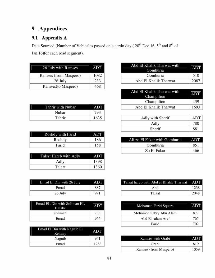
81
9 Appendices
9.1 Appendix A
Data Sourced (Number of Vehicales passed on a certin day ( 28th Dec.16, 5th and 8th of
Jan.16)for each road segment).
26 July with Ramses ADT
Abd El Khalik Tharwat with Gomhuria
ADT
Ramses (from Maspero) 1082
Gomhuria 510
26 July 233
Abd El Khalik Tharwat 2087
Ramses(to Maspero) 468
Abd El Khalik Tharwat with
Champilion ADT
Champilion 439
Tahrir with Nubar ADT
Abd El Khalik Tharwat 1693
Nubar 793
Tahrir 1635
Adly with Sherif ADT
Adly 780
Sherif 881
Roshdy with Farid ADT
Roshdy 186
Ali zo El Fakar with Gomhuria ADT
Farid 158
Gomhuria 851
Zo El Fakar 466
Talsst Hareb with Adly ADT
Adly 1398
Talaat 1360
Emad El Din with 26 July ADT
Talaat hareb with Abd el Khalik Tharwat ADT
Emad 887
Abd 1238
26 July 991
Talaat 2048
Emad EL Din with Soliman EL
Halabe ADT
Mohamed Farid Square ADT
soliman 738
Mohamed Sabry Abu Alam 877
Emad 955
Abd El salam Aref 765
Farid 702
Emad El Din with Naguib El Rehany
ADT
Naguib 941
Ramses with Orabi ADT
Emad 1283
Orabi 819
Ramses (from Maspero) 1059

82
Qasr El Nile with Gomhuria ADT
Ramses(to Maspero) 489
Gomhuria 851
Qasr 1536
Adly with Mohamed Farid ADT
Farid 1141
Mostafa Kamel square ADT
Adly 1224
Farid 982
Qasr 1177
83
Series from Lund University
Department of Physical Geography and Ecosystem Science
Master Thesis in Geographical Information Science
1. Anthony Lawther: The application of GIS-based binary logistic regression for
slope failure susceptibility mapping in the Western Grampian Mountains,
Scotland (2008).
2. Rickard Hansen: Daily mobility in Grenoble Metropolitan Region, France.
Applied GIS methods in time geographical research (2008).
3. Emil Bayramov: Environmental monitoring of bio-restoration activities using
GIS and Remote Sensing (2009).
4. Rafael Villarreal Pacheco: Applications of Geographic Information Systems
as an analytical and visualization tool for mass real estate valuation: a case
study of Fontibon District, Bogota, Columbia (2009).
5. Siri Oestreich Waage: a case study of route solving for oversized transport:
The use of GIS functionalities in transport of transformers, as part of
maintaining a reliable power infrastructure (2010).
6. Edgar Pimiento: Shallow landslide susceptibility – Modelling and validation
(2010).
7. Martina Schäfer: Near real-time mapping of floodwater mosquito breeding
sites using aerial photographs (2010).
8. August Pieter van Waarden-Nagel: Land use evaluation to assess the outcome
of the programme of rehabilitation measures for the river Rhine in the
Netherlands (2010).
9. Samira Muhammad: Development and implementation of air quality data mart
for Ontario, Canada: A case study of air quality in Ontario using OLAP tool.
(2010).
10. Fredros Oketch Okumu: Using remotely sensed data to explore spatial and
temporal relationships between photosynthetic productivity of vegetation and
malaria transmission intensities in selected parts of Africa (2011).
84
11. Svajunas Plunge: Advanced decision support methods for solving diffuse
water pollution problems (2011).
12. Jonathan Higgins: Monitoring urban growth in greater Lagos: A case study
using GIS to monitor the urban growth of Lagos 1990 - 2008 and produce
future growth prospects for the city (2011).
13. Mårten Karlberg: Mobile Map Client API: Design and Implementation for
Android (2011).
14. Jeanette McBride: Mapping Chicago area urban tree canopy using color
infrared imagery (2011).
15. Andrew Farina: Exploring the relationship between land surface temperature
and vegetation abundance for urban heat island mitigation in Seville, Spain
(2011).
16. David Kanyari: Nairobi City Journey Planner: An online and a Mobile
Application (2011).
17. Laura V. Drews: Multi-criteria GIS analysis for siting of small wind power
plants - A case study from Berlin (2012).
18. Qaisar Nadeem: Best living neighborhood in the city - A GIS based multi
criteria evaluation of ArRiyadh City (2012).
19. Ahmed Mohamed El Saeid Mustafa: Development of a photo voltaic building
rooftop integration analysis tool for GIS for Dokki District, Cairo, Egypt
(2012).
20. Daniel Patrick Taylor: Eastern Oyster Aquaculture: Estuarine Remediation via
Site Suitability and Spatially Explicit Carrying Capacity Modeling in
Virginia’s Chesapeake Bay (2013).
21. Angeleta Oveta Wilson: A Participatory GIS approach to unearthing
Manchester’s Cultural Heritage ‘gold mine’ (2013).
22. Ola Svensson: Visibility and Tholos Tombs in the Messenian Landscape: A
Comparative Case Study of the Pylian Hinterlands and the Soulima Valley
(2013).
23. Monika Ogden: Land use impact on water quality in two river systems in
South Africa (2013).
85
24. Stefan Rova: A GIS based approach assessing phosphorus load impact on Lake
Flaten in Salem, Sweden (2013).
25. Yann Buhot: Analysis of the history of landscape changes over a period of 200
years. How can we predict past landscape pattern scenario and the impact on
habitat diversity? (2013).
26. Christina Fotiou: Evaluating habitat suitability and spectral heterogeneity
models to predict weed species presence (2014).
27. Inese Linuza: Accuracy Assessment in Glacier Change Analysis (2014).
28. Agnieszka Griffin: Domestic energy consumption and social living standards: a
GIS analysis within the Greater London Authority area (2014).
29. Brynja Guðmundsdóttir: Detection of potential arable land with remote
sensing and GIS - A Case Study for Kjósarhreppur (2014).
30. Oleksandr Nekrasov: Processing of MODIS Vegetation Indices for analysis of
agricultural droughts in the southern Ukraine between the years 2000-2012
(2014).
31. Sarah Tressel: Recommendations for a polar Earth science portal
in the context of Arctic Spatial Data Infrastructure (2014).
32. Caroline Gevaert: Combining Hyperspectral UAV and Multispectral
Formosat-2 Imagery for Precision Agriculture Applications (2014).
33. Salem Jamal-Uddeen: Using GeoTools to implement the multi-criteria
evaluation analysis - weighted linear combination model (2014).
34. Samanah Seyedi-Shandiz: Schematic representation of geographical railway
network at the Swedish Transport Administration (2014).
35. Kazi Masel Ullah: Urban Land-use planning using Geographical Information
System and analytical hierarchy process: case study Dhaka City (2014).
36. Alexia Chang-Wailing Spitteler: Development of a web application based on
MCDA and GIS for the decision support of river and floodplain rehabilitation
projects (2014).
37. Alessandro De Martino: Geographic accessibility analysis and evaluation of
potential changes to the public transportation system in the City of Milan
(2014).
86
38. Alireza Mollasalehi: GIS Based Modelling for Fuel Reduction Using
Controlled Burn in Australia. Case Study: Logan City, QLD (2015).
39. Negin A. Sanati: Chronic Kidney Disease Mortality in Costa Rica;
Geographical Distribution, Spatial Analysis and Non-traditional Risk Factors
(2015).
40. Karen McIntyre: Benthic mapping of the Bluefields Bay fish sanctuary,
Jamaica (2015).
41. Kees van Duijvendijk: Feasibility of a low-cost weather sensor network for
agricultural purposes: A preliminary assessment (2015).
42. Sebastian Andersson Hylander: Evaluation of cultural ecosystem services
using GIS (2015).
43. Deborah Bowyer: Measuring Urban Growth, Urban Form and Accessibility as
Indicators of Urban Sprawl in Hamilton, New Zealand (2015).
44. Stefan Arvidsson: Relationship between tree species composition and
phenology extracted from satellite data in Swedish forests (2015).
45. Damián Giménez Cruz: GIS-based optimal localisation of beekeeping in rural
Kenya (2016).
46. Alejandra Narváez Vallejo: Can the introduction of the topographic indices in
LPJ-GUESS improve the spatial representation of environmental variables?
(2016).
47. Anna Lundgren: Development of a method for mapping the highest coastline
in Sweden using breaklines extracted from high resolution digital elevation
models (2016).
48. Oluwatomi Esther Adejoro: Does location also matter? A spatial analysis of
social achievements of young South Australians (2016).
49. Hristo Dobrev Tomov: Automated temporal NDVI analysis over the Middle
East for the period 1982 - 2010 (2016).
50. Vincent Muller: Impact of Security Context on Mobile Clinic Activities
A GIS Multi Criteria Evaluation based on an MSF Humanitarian Mission in
Cameroon (2016).
87
51. Gezahagn Negash Seboka: Spatial Assessment of NDVI as an Indicator of
Desertification in Ethiopia using Remote Sensing and GIS (2016).
52. Holly Buhler: Evaluation of Interfacility Medical Transport Journey Times in
Southeastern British Columbia. (2016).
53. Lars Ole Grottenberg: Assessing the ability to share spatial data between
emergency management organisations in the High North (2016).
54. Sean Grant: The Right Tree in the Right Place: Using GIS to Maximize the
Net Benefits from Urban Forests (2016).
55. Irshad Jamal: Multi-Criteria GIS Analysis for School Site Selection in Gorno-
Badakhshan Autonomous Oblast, Tajikistan (2016).
56. Fulgencio Sanmartín: Wisdom-volkano: A novel tool based on open GIS and
time-series visualization to analyse and share volcanic data (2016).
57. Nezha Acil: Remote sensing-based monitoring of snow cover dynamics and its
influence on vegetation growth in the Middle Atlas Mountains (2016).
58. Julia Hjalmarsson: A Weighty Issue: Estimation of Fire Size with
Geographically Weighted Logistic Regression (2016).
59. Mathewos Tamiru Amato: Using multi-criteria evaluation and GIS for chronic
food and nutrition insecurity indicators analysis in Ethiopia (2016).