Accepted Manuscript

Benchmarking state-of-the-art classification algorithms for creditscoring: An update of research

Stefan Lessmann , Bart Baesens , Hsin-Vonn Seow ,Lyn C. Thomas

PII: S0377-2217(15)00420-8DOI: 10.1016/j.ejor.2015.05.030Reference: EOR 12954

To appear in: European Journal of Operational Research

Received date: 23 December 2013Revised date: 9 March 2015Accepted date: 11 May 2015

Please cite this article as: Stefan Lessmann , Bart Baesens , Hsin-Vonn Seow , Lyn C. Thomas ,Benchmarking state-of-the-art classification algorithms for credit scoring: An update of research, Euro-pean Journal of Operational Research (2015), doi: 10.1016/j.ejor.2015.05.030

This is a PDF file of an unedited manuscript that has been accepted for publication. As a serviceto our customers we are providing this early version of the manuscript. The manuscript will undergocopyediting, typesetting, and review of the resulting proof before it is published in its final form. Pleasenote that during the production process errors may be discovered which could affect the content, andall legal disclaimers that apply to the journal pertain.

ACCEPTED MANUSCRIPT

ACCEPTED MANUSCRIP

T

1

Highlights Large-scale benchmark of 41 classifiers across 8 real-word credit scoring data sets.

Introduction of ensemble selection routines to the credit scoring community.

Analysis of 6 established and novel indicators to measure scorecard accuracy.

Assessment of the financial impact of different scorecards.

ACCEPTED MANUSCRIPT

ACCEPTED MANUSCRIP

T

2

Benchmarking state-of-the-art classification algorithms for credit

scoring: An update of research

Stefan Lessmanna,*

, Bart Baesensbc

, Hsin-Vonn Seowd , Lyn C. Thomas

c

a School of Business and Economics, Humboldt-University of Berlin

b Department of Decision Sciences & Information Management, Catholic University of Leuven

c School of Management, University of Southampton, Highfield, Southampton, SO17 1BJ, United Kingdom

d Nottingham University Business School, University of Nottingham-Malaysia Campus

Abstract

Many years have passed since Baesens et al. published their benchmarking study of

classification algorithms in credit scoring [Baesens, B., Van Gestel, T., Viaene, S., Stepanova,

M., Suykens, J., & Vanthienen, J. (2003). Benchmarking state-of-the-art classification

algorithms for credit scoring. Journal of the Operational Research Society, 54(6), 627-635.].

The interest in prediction methods for scorecard development is unbroken. However, there

have been several advancements including novel learning methods, performance measures

and techniques to reliably compare different classifiers, which the credit scoring literature

does not reflect. To close these research gaps, we update the study of Baesens et al. and

compare several novel classification algorithms to the state-of-the-art in credit scoring. In

addition, we examine the extent to which the assessment of alternative scorecards differs

across established and novel indicators of predictive accuracy. Finally, we explore whether

more accurate classifiers are managerial meaningful. Our study provides valuable insight for

professionals and academics in credit scoring. It helps practitioners to stay abreast of technical

advancements in predictive modeling. From an academic point of view, the study provides an

independent assessment of recent scoring methods and offers a new baseline to which future

approaches can be compared.

Keywords: Data Mining, Credit Scoring, OR in banking, Forecasting benchmark

* Corresponding author: Tel.: +49.30.2093.5742, Fax: +49.30.2093.5741, E-Mail: stefan.lessmann@hu-

berlin.de. a

School of Business and Economics, Humboldt-University of Berlin, Unter den Linden 6, 10099 Berlin,

Germany b

Department of Decision Sciences & Information Management, Catholic University of Leuven, Naamsestraat

69, B-3000 Leuven, Belgium c

School of Management, University of Southampton, Highfield, Southampton, SO17 1BJ, United Kingdom d Nottingham University Business School, University of Nottingham-Malaysia Campus, Jalan Broga, 43500

Semenyih, Selangor Darul Ehsan, Malaysia

ACCEPTED MANUSCRIPT

ACCEPTED MANUSCRIP

T

3

1 Introduction

Credit scoring is concerned with developing empirical models to support decision making

in the retail credit business (Crook, et al., 2007). This sector is of considerable economic

importance. For example, the volume of consumer loans held by banks in the US was

$1,132bn in 2013; compared to $1,541bn in the corporate business.1 In the UK, loans and

mortgages to individuals were even higher than corporate loans in 2012 (£11,676m c.f.

£10,388m).2 These figures indicate that financial institutions require formal tools to inform

lending decisions.

A credit score is a model-based estimate of the probability that a borrower will show some

undesirable behavior in the future. In application scoring, for example, lenders employ

predictive models, called scorecards, to estimate how likely an applicant is to default. Such

PD (probability of default) scorecards are routinely developed using classification algorithms

(e.g., Hand & Henley, 1997). Many studies have examined the accuracy of alternative

classifiers. One of the most comprehensive classifier comparisons to date is the benchmarking

study of Baesens, et al. (2003).

Albeit much research, we argue that the credit scoring literature does not reflect several

recent advancements in predictive learning. For example, the development of selective

multiple classifier systems that pool different algorithms and optimize their weighting through

heuristic search represents an important trend in machine learning (e.g., Partalas, et al., 2010).

Yet, no attempt has been made to systematically examine the potential of such approach for

credit scoring. More generally, recent advancements concern three dimensions: i) novel

classification algorithms to develop scorecards (e.g., extreme learning machines, rotation

forest, etc.), ii) novel performance measures to assess scorecards (e.g., the H-measure or the

partial Gini coefficient), and iii) statistical hypothesis tests to compare scorecard performance

(e.g., García, et al., 2010). An analysis of the PD modeling literature confirms that these

developments have received little attention in credit scoring, and reveals further limitations of

previous studies; namely i) using few and/or small data sets, ii) not comparing different state-

of-the-art classifiers to each other, and iii) using only a small set of conceptually similar

accuracy indicators. We elaborate on these issues in Section 2.

The above research gaps warrant an update of Baesens, et al. (2003). Therefore, the

motivation of this paper is to provide a holistic view of the state-of-the-art in predictive

1 Data from the Federal Reserve Board, H8, Assets and Liabilities of Commercial Banks in the United States

(http://www.federalreserve.gov/releases/h8/current/). 2 Data from ONS Online, SDQ7: Assets, Liabilities and Transactions in Finance Leasing, Factoring and Credit

Granting: 1st quarter 2012 (http://www.ons.gov.uk).

ACCEPTED MANUSCRIPT

ACCEPTED MANUSCRIP

T

4

modeling and how it can support decision making in the retail credit business. In pursuing this

objective, we make the following contributions: First, we perform a large scale benchmark of

41 classification methods across eight credit scoring data sets. Several of the classifiers are

new to the community and for the first time assessed in credit scoring. Second, using the

principles of cost-sensitive learning, we shed light on the link between the (statistical)

accuracy of scorecard predictions and the business value of a scorecard. This offers some

guidance whether deploying advanced – more accurate – classification models is

economically sensible. Third, we examine the correspondence between empirical results

obtained using different accuracy indicators. In particular, we clarify the reliability of

scorecard comparisons in the light of recently identified limitations of the area under a

receiver operating characteristics curve (Hand, 2009; Hand & Anagnostopoulos, 2013).

Finally, we illustrate the use of advanced nonparametric testing procedures to secure

empirical findings and, thereby, offer guidance how to organize future classifier comparisons.

In the remainder of the paper we first review related work in Section 2. We then

summarize the classifiers that we compare (Section 3) and describe our experimental design

(Section 4). Next, we discuss empirical results (Section 5). Section 6 concludes the paper. The

online appendix3 provides a detailed description of the classification algorithms and additional

results.

2 Literature review

Much literature explores the development, application, and evaluation of predictive

decision support models in the credit industry (see, Crook, et al., 2007; Kumar & Ravi, 2007

for reviews). Such models estimate credit worthiness based on a set of explanatory variables.

Corporate risk models employ data from balance sheets, financial ratios, or macro-economic

indicators, whereas retail models use data from application forms, customer demographics,

and transactional data from the customer history (e.g., Thomas, 2010). The differences

between the types of variables suggest that specific modeling challenges arise in consumer as

opposed to corporate credit scoring. Thus, many studies focus on either the corporate or the

retail business. The latter is the focus of this paper.

A variety of prediction tasks arise in consumer credit risk modeling. The Basel II Capital

Accord requires financial institutions to estimate, respectively, the probability of default (PD),

the exposure at default (EAD), and the loss given default (LGD). EAD and LGD models have

recently become a popular research topic (e.g., Calabrese, 2014; Yao, et al., 2015). PD models

3 Available at: (URL will be inserted by Elsevier when available)

ACCEPTED MANUSCRIPT

ACCEPTED MANUSCRIP

T

5

are especially well researched and continue to attract much interest. Topical research question

include, for example, how to update PD scorecards in the face of new information (Hofer,

2015; Sohn & Ju, 2014). The prevailing methods to develop PD models are classification and

survival analysis. The latter facilitates estimating not only whether but also when a customer

defaults (e.g., Tong, et al., 2012). In addition, a special type of survival model called mixture

cure model facilitates predicting multiple events of interest; for example default and early

repayment (e.g., Dirick, et al., 2015; Liu, et al., 2015). Classification analysis, on the other

hand, represents the classic approach and benefits from an unmatched variety of modeling

methods.

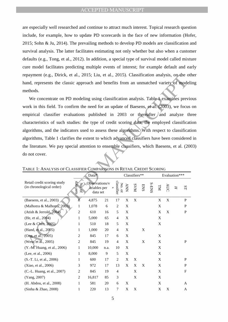
We concentrate on PD modeling using classification analysis. Table 1 examines previous

work in this field. To confirm the need for an update of Baesens, et al. (2003), we focus on

empirical classifier evaluations published in 2003 or thereafter and analyze three

characteristics of such studies: the type of credit scoring data, the employed classification

algorithms, and the indicators used to assess these algorithms. With respect to classification

algorithms, Table 1 clarifies the extent to which advanced classifiers have been considered in

the literature. We pay special attention to ensemble classifiers, which Baesens, et al. (2003)

do not cover.

TABLE 1: ANALYSIS OF CLASSIFIER COMPARISONS IN RETAIL CREDIT SCORING

Retail credit scoring study

(in chronological order)

Data* Classifiers** Evaluation***

No

. of

data sets

Observations/v

ariables per

data set

No

. of

classifier

s

AN

N

SV

M

EN

S

S-E

NS

TM

AU

C

H

ST

(Baesens, et al., 2003) 8 4,875 21 17 X X

X X P

(Malhotra & Malhotra, 2003) 1 1,078 6 2 X

X

P

(Atish & Jerrold, 2004) 2 610 16 5 X

X X P

(He, et al., 2004) 1 5,000 65 4 X

X

(Lee & Chen, 2005) 1 510 18 5 X

X

(Hand, et al., 2005) 1 1,000 20 4 X

X

(Ong, et al., 2005) 2 845 17 6 X

X

(West, et al., 2005) 2 845 19 4 X

X

X

P

(Y.-M. Huang, et al., 2006) 1 10,000 n.a. 10 X

X

(Lee, et al., 2006) 1 8,000 9 5 X

X

(S.-T. Li, et al., 2006) 1 600 17 2 X X

X

P

(Xiao, et al., 2006) 3 972 17 13 X X X

X

P

(C.-L. Huang, et al., 2007) 2 845 19 4

X

X

F

(Yang, 2007) 2 16,817 85 3

X

X

(H. Abdou, et al., 2008) 1 581 20 6 X

X

A

(Sinha & Zhao, 2008) 1 220 13 7 X X

X X A

ACCEPTED MANUSCRIPT

ACCEPTED MANUSCRIP

T

6

(C.-F. Tsai & Wu, 2008) 3 793 16 3 X

X

X

P

(Xu, et al., 2009) 1 690 15 4

X

X

(Yu, et al., 2008) 1 653 13 7

X X X

(H. A. Abdou, 2009) 1 1,262 25 3

X

(Bellotti & Crook, 2009) 1 25,000 34 4

X

X

(Chen, et al., 2009) 1 2,000 15 5

X

X

(Nanni & Lumini, 2009) 3 793 16 16 X X X X X

(Šušteršič, et al., 2009) 1 581 84 2 X

X

(M.-C. Tsai, et al., 2009) 1 1,877 14 4 X

X

Q

(Yu, et al., 2009) 3 959 16 10 X X X

X X P

(J. Zhang, et al., 2009) 1 1,000 102 4

X

(Hsieh & Hung, 2010) 1 1,000 20 4 X X X

X

(Martens, et al., 2010) 1 1,000 20 4

X

X

(Twala, 2010) 2 845 18 5

X

X

(Yu, et al., 2010) 1 1,225 14 8 X X X

X

P

(D. Zhang, et al., 2010) 2 845 17 11 X X X

X

(Zhou, et al., 2010) 2 1,113 17 25 X X X X X

(J. Li, et al., 2011) 2 845 17 11

X

X

(Finlay, 2011) 2 104,649 47 18 X

X

X

P

(Ping & Yongheng, 2011) 2 845 17 4 X X

X

(Wang, et al., 2011) 3 643 17 13 X X X

X

(Yap, et al., 2011) 1 2,765 4 3

X

(Yu, et al., 2011) 2 845 17 23 X X

X

(Akkoc, 2012) 1 2,000 11 4 X

X X

(Brown & Mues, 2012) 5 2,582 30 9 X X X

X F/P

(Hens & Tiwari, 2012) 2 845 19 4

X

X

(S. Li, et al., 2012) 2 672 15 5

X X

X

(Marqués, et al., 2012a) 4 836 20 35 X X X

X

F/P

(Marqués, et al., 2012b) 4 836 20 17 X X X

X X F/P

(Kruppa, et al., 2013) 1 65,524 17 5

X

X

(Abellán & Mantas, 2014) 3 793 16 5 X X X A

(C.-F. Tsai, 2014) 3 793 16 21 X X X F/P

Mean / counts 1.9 6,167 24 7.8 30 24 18 3 40 10 0 17

* We report the mean of observations and independent variables for studies that employ multiple data sets.

Eight studies mix retail and corporate credit data. Table 1 considers the retail data sets only.

** Abbreviations have the following meaning: ANN=Artificial neural network, SVM=Support vector machine,

ENS=Ensemble classifier, S-ENS=Selective Ensemble (e.g., Partalas, et al., 2010).

*** Abbreviations have the following meaning: TM=Threshold metric (e.g., classification error, true positive

rate, costs, etc.), AUC=Area under receiver operating characteristics curve, H=H-measure (Hand, 2009),

ST=Statistical hypothesis testing. We use the following codes to report the type of statistical test used for

classifier comparisons: P=Pairwise comparison (e.g., paired t-test), A=Analysis of variance, F=Friedman

test, F/P=Friedman test together with post-hoc test (e.g., Demšar, 2006), Q=Press’s Q statistic.

Five conclusions emerge from Table 1. First, it is common practice to use a small number

of data sets (1.9 on average), many of which contain only few cases and/or independent

variables. This appears inappropriate. Using multiple data sets (e.g., data from different

ACCEPTED MANUSCRIPT

ACCEPTED MANUSCRIP

T

7

companies) facilitates examining the robustness of a scorecard toward environmental

conditions. Also, real-world credit data sets are typically large and high-dimensional. The data

used in classifier comparisons should be similar to ensure the external validity of empirical

results (e.g., Finlay, 2011; Hand, 2006).

Second, the number of classifiers per study varies considerably. This can be explained

with common research setups. Studies with fewer classifiers propose a novel algorithm and

compare it to some reference methods (e.g., Abellán & Mantas, 2014; Akkoc, 2012; Yang,

2007). Studies with several classifiers often pair algorithms and ensemble strategies in a

factorial design (e.g., Marqués, et al., 2012a; Nanni & Lumini, 2009; Wang, et al., 2011).

Both setups have limitations. The latter focuses on preselected methods and omits a

systematic comparison of several state-of-the-art classifiers. Studies that introduce novel

classifiers may be over-optimistic because i) the developers of a new method are more adept

with their approach than external users, and ii) the new method may have been tuned more

intensively than reference methods (Hand, 2006; Thomas, 2010). Independent benchmarks

complement the other setups in that they compare many classifiers without prior hypotheses

which method excels.

Third, most studies rely on a single performance measure or measures of the same type. In

general, performance measures split into three types. Those that assess the discriminatory

ability of the scorecard (e.g., AUC); those that assess the accuracy of the scorecard’s

probability predictions (e.g., Brier Score) and those that assess the correctness of the

scorecards’ categorical predictions (e.g., classification error). Different types of indicators

embody a different notion of classifier performance. Few studies mix evaluation measures

from different categories. For example, none of the reviewed studies uses the Brier Score to

assess the accuracy of probabilistic predictions. This misses an important aspect of scorecard

performance because financial institutions require PD estimates that are not only accurate but

also well calibrated. Furthermore, no previous study uses the H-measure, although it

overcomes conceptual shortcomings of the AUC (Hand, 2009). It is thus beneficial to also

consider the H-measure in classifier comparisons and, more generally, to assess scorecards

with conceptually different performance measures.

Fourth, statistical hypothesis testing is often neglected or employed inappropriately.

Common mistakes include using parametric tests (e.g., the t-test) or performing multiple

comparisons without controlling the family-wise error level (shown by a ‘P’ in the last

column of Table 1). The approaches are inappropriate because the assumptions of parametric

tests are violated in classifier comparisons (Demšar, 2006). Similarly, pairwise comparisons

ACCEPTED MANUSCRIPT

ACCEPTED MANUSCRIP

T

8

without p-value adjustment increase the actual probability of Type-I errors beyond the stated

level of 𝛼 (e.g., García, et al., 2010).

Last, only two studies employ selective ensembles and they use rather simple approaches

(Yu, et al., 2008; Zhou, et al., 2010). Selective ensembles are an active field of research and

have shown promising results (e.g., Partalas, et al., 2010). The lack of a systematic evaluation

of selective ensembles in credit scoring might thus be an important research gap.

From the literature review, we conclude that an update of Baesens, et al. (2003) is needed.

This study overcomes several of the above issues through i) conducting a large-scale

comparison of many established and novel classifiers including selective ensembles, ii) using

multiple data sets of considerable size, iii) considering several conceptually different

performance criteria, and iv) using suitable statistical testing procedures.

3 Classification algorithms for scorecard construction

We illustrate the development of a credit scorecard in the context of application scoring.

Let 𝒙 = (𝑥1, 𝑥2, … , 𝑥𝑚) ∈ ℝ𝑚 be an m-dimensional vector with application characteristics,

and let 𝑦 ∈ {−1; +1} be a binary variable that distinguishes good (𝑦 = −1) and bad loans

(𝑦 = +1). A scorecard estimates the (posterior) probability 𝑝(+|𝒙𝑖) that a default event will

be observed for loan i; where 𝑝(+|𝒙) is a shorthand form of 𝑝(𝑦 = +1|𝒙). To decide on an

application, a credit analyst compares the estimated default probability to a threshold 𝜏;

approving the loan if 𝑝(+|𝒙) ≤ 𝜏, and rejecting it otherwise. The task to estimate 𝑝(+|𝒙)

belongs to the field of classification (e.g., Hand & Henley, 1997). A scorecard is a

classification model that results from applying a classification algorithm to a data set 𝐷 =

(𝑦𝑖, 𝒙𝑖)𝑖=1𝑛 of past loans.

This study compares 41 different classification algorithms. Our selection draws inspiration

from previous studies (e.g., Baesens, et al., 2003; Finlay, 2011; Verbeke, et al., 2012) and

covers several different approaches (linear/nonlinear, parametric/non-parametric, etc.). The

algorithms split into individual and ensemble classifiers. The eventual scorecard consists of a

single classification model in the first group. Ensemble classifiers integrate the prediction of

multiple models, called base models. We distinguish homogeneous ensembles, which create

the base models using the same algorithm, and heterogeneous ensembles, which employ

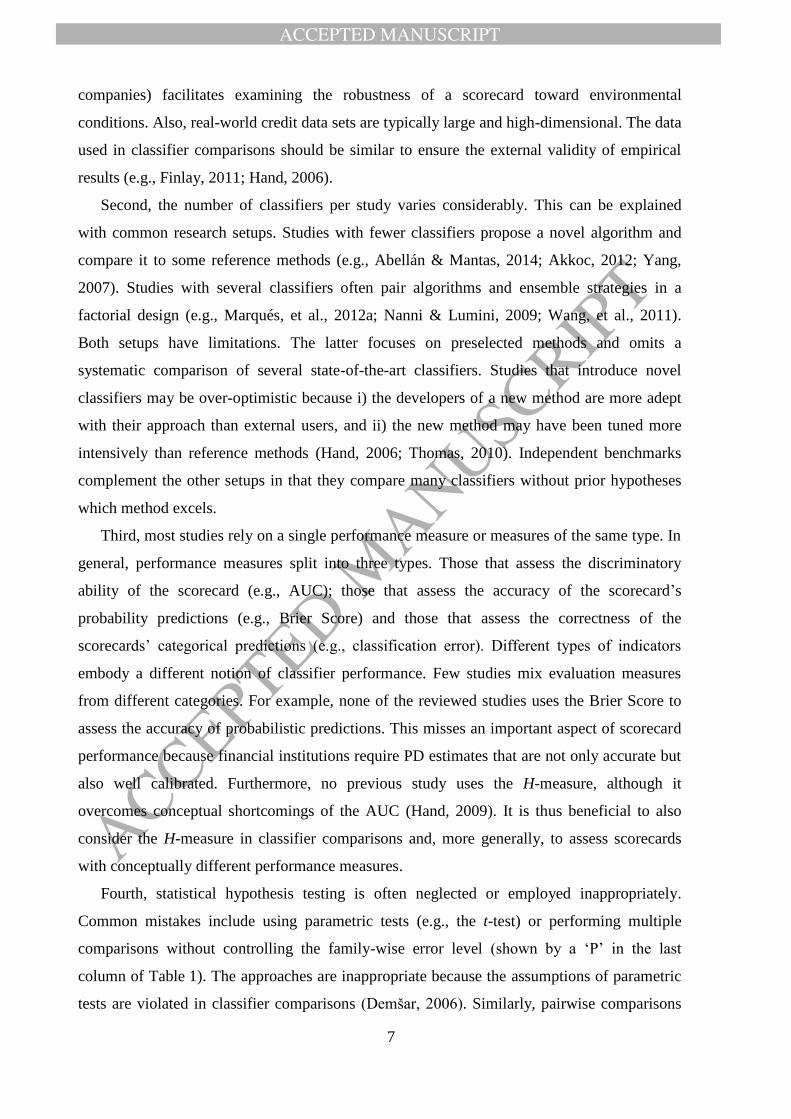
different algorithms. Figure 1 illustrates the modeling process using different classifiers.

ACCEPTED MANUSCRIPT

ACCEPTED MANUSCRIP

T

9

Classification models1

Validation set predictions

Heterogeneous ensemblealgorithm

Individual classification

algorithm

Homogeneousensemble algorithm

Training set

Validation set

Testset

DataTrain

classifier

Test set prediction

Train ensemble

Ensemble models2

Applymodel

Apply model

Benchmarkclassifier

1 Individual classifier & homogeneous ensemble classifier2 Heterogeneous ensemble classifier

Figure 1: Classifier development and evaluation process

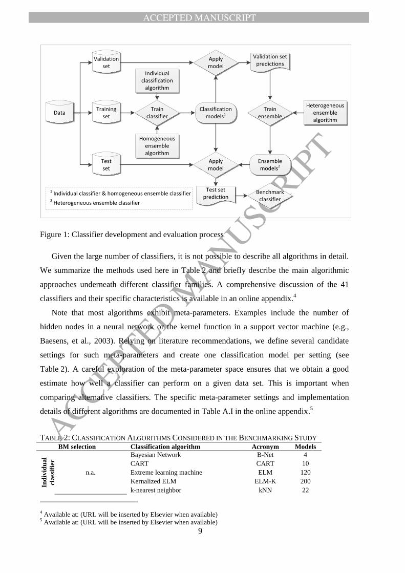
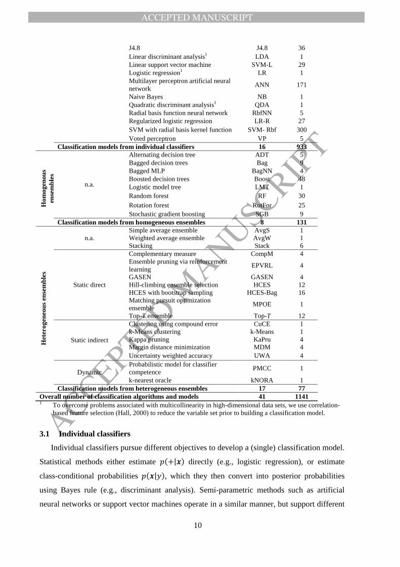
Given the large number of classifiers, it is not possible to describe all algorithms in detail.

We summarize the methods used here in Table 2 and briefly describe the main algorithmic

approaches underneath different classifier families. A comprehensive discussion of the 41

classifiers and their specific characteristics is available in an online appendix.4

Note that most algorithms exhibit meta-parameters. Examples include the number of

hidden nodes in a neural network or the kernel function in a support vector machine (e.g.,

Baesens, et al., 2003). Relying on literature recommendations, we define several candidate

settings for such meta-parameters and create one classification model per setting (see

Table 2). A careful exploration of the meta-parameter space ensures that we obtain a good

estimate how well a classifier can perform on a given data set. This is important when

comparing alternative classifiers. The specific meta-parameter settings and implementation

details of different algorithms are documented in Table A.I in the online appendix.5

TABLE 2: CLASSIFICATION ALGORITHMS CONSIDERED IN THE BENCHMARKING STUDY BM selection Classification algorithm Acronym Models

Ind

ivid

ua

l

cla

ssif

ier

(16

alg

ori

thm

s

an

d 9

33

mo

del

s in

tota

l)

n.a.

Bayesian Network B-Net 4

CART CART 10

Extreme learning machine ELM 120

Kernalized ELM ELM-K 200

k-nearest neighbor kNN 22

4 Available at: (URL will be inserted by Elsevier when available)

5 Available at: (URL will be inserted by Elsevier when available)

ACCEPTED MANUSCRIPT

ACCEPTED MANUSCRIP

T

10

J4.8 J4.8 36

Linear discriminant analysis1 LDA 1

Linear support vector machine SVM-L 29

Logistic regression1 LR 1

Multilayer perceptron artificial neural

network ANN 171

Naive Bayes NB 1

Quadratic discriminant analysis1 QDA 1

Radial basis function neural network RbfNN 5

Regularized logistic regression LR-R 27

SVM with radial basis kernel function SVM- Rbf 300

Voted perceptron VP 5

Classification models from individual classifiers 16 933

Ho

mo

gen

ou

s

ense

mb

les

n.a.

Alternating decision tree ADT 5

Bagged decision trees Bag 9

Bagged MLP BagNN 4

Boosted decision trees Boost 48

Logistic model tree LMT 1

Random forest RF 30

Rotation forest RotFor 25

Stochastic gradient boosting SGB 9

Classification models from homogeneous ensembles 8 131

Het

ero

gen

eou

s en

sem

ble

s

n.a.

Simple average ensemble AvgS 1

Weighted average ensemble AvgW 1

Stacking

Stack 6

Static direct

Complementary measure CompM 4

Ensemble pruning via reinforcement

learning EPVRL 4

GASEN

GASEN 4

Hill-climbing ensemble selection

HCES 12

HCES with bootstrap sampling

HCES-Bag 16

Matching pursuit optimization

ensemble MPOE 1

Top-T ensemble Top-T 12

Static indirect

Clustering using compound error CuCE 1

k-Means clustering

k-Means 1

Kappa pruning KaPru 4

Margin distance minimization

MDM 4

Uncertainty weighted accuracy UWA 4

Dynamic

Probabilistic model for classifier

competence PMCC 1

k-nearest oracle

kNORA 1

Classification models from heterogeneous ensembles 17 77

Overall number of classification algorithms and models 41 1141 1 To overcome problems associated with multicollinearity in high-dimensional data sets, we use correlation-

based feature selection (Hall, 2000) to reduce the variable set prior to building a classification model.

3.1 Individual classifiers

Individual classifiers pursue different objectives to develop a (single) classification model.

Statistical methods either estimate 𝑝(+|𝒙) directly (e.g., logistic regression), or estimate

class-conditional probabilities 𝑝(𝒙|𝑦), which they then convert into posterior probabilities

using Bayes rule (e.g., discriminant analysis). Semi-parametric methods such as artificial

neural networks or support vector machines operate in a similar manner, but support different

ACCEPTED MANUSCRIPT

ACCEPTED MANUSCRIP

T

11

functional forms and require the modeler to select one specification a priori. The parameters

of the resulting model are estimated using nonlinear optimization. Tree-based methods

recursively partition a data set so as to separate good and bad loans through a sequence of

tests (e.g., is loan amount > threshold). This produces a set of rules that facilitate assessing

new loan applications. The specific covariates and threshold values to branch a node follow

from minimizing indicators of node impurity such as the Gini coefficient or information gain

(e.g., Baesens, et al., 2003).

3.2 Homogeneous ensemble classifiers

Homogeneous ensemble classifiers pool the predictions of multiple base models. Much

empirical and theoretical evidence has shown that model combination increases predictive

accuracy (e.g., Finlay, 2011; Paleologo, et al., 2010). Homogeneous ensemble learners create

the base models in an independent or dependent manner. For example, the bagging algorithm

derives independent base models from bootstrap samples of the original data (Breiman, 1996).

Boosting algorithms, on the other hand, grow an ensemble in a dependent fashion. They

iteratively add base models that are trained to avoid the errors of the current ensemble (Freund

& Schapire, 1996). Several extensions of bagging and boosting have been proposed in the

literature (e.g., Breiman, 2001; Friedman, 2002; Rodriguez, et al., 2006). The common

denominator of homogeneous ensembles is that they develop the base models using the same

classification algorithm.

3.3 Heterogeneous ensemble classifiers

Heterogeneous ensembles also combine multiple classification models but create these

models using different classification algorithms. In that sense, they encompass individual

classifiers and homogeneous ensembles as special cases (see Figure 1). The idea is that

different algorithms have different views about the same data and can complement each other.

Recently, heterogeneous ensembles that prune some base models prior to combination have

attracted much research (e.g., Partalas, et al., 2010). This study pays special attention to such

selective ensembles because they have received little attention in credit scoring (see Table 1).

Generally speaking, ensemble modeling involves two steps: base models development and

forecast combination. Selective ensembles add a third step. After creating a pool of base

models, they search the space of available base models for a ‘suitable’ model subset that

enters the ensemble. An interesting feature of this framework is that the search problem can

be approached in many different ways. Hence, much research concentrates on developing

different ensemble selection strategies (e.g., Caruana, et al., 2006; Partalas, et al., 2009).

ACCEPTED MANUSCRIPT

ACCEPTED MANUSCRIP

T

12

Selective ensembles split into static and dynamic approaches, depending on how they

organize the selection step. Static approaches perform the base model search once. Dynamic

approaches repeat the selection step for every case. More specifically, using the independent

variables of a case, they compose a tailor-made ensemble from the model library. Dynamic

ensemble selection might violate regulatory requirements in credit scoring because one would

effectively use different scorecards for different customers. In view of this, we focus on static

methods, but consider two dynamic approaches (Ko, et al., 2008; Woloszynski & Kurzynski,

2011) as benchmarks.

The goal of an ensemble is to predict with high accuracy. To achieve this, many selective

ensembles chose base models so as to maximize predictive accuracy (e.g., Caruana, et al.,

2006). We call this a direct approach. Indirect approaches, on the other hand, optimize the

diversity among base models, which is another determinant of ensemble success (e.g.,

Partalas, et al., 2010).

4 Experimental Setup

4.1 Credit scoring data sets

The empirical evaluation includes eight retail credit scoring data sets. The data sets

Australian credit (AC) and German credit (GC) from the UCI Library (Lichman, 2013) and

the Th02 data set from Thomas, et al. (2002) have been used in several previous papers (see

Section 2). Three other data sets, Bene-1, Bene-2, and UK, also used in Baesens, et al. (2003),

were collected from major financial institutions in the Benelux and UK, respectively. Note

that our data set UK encompasses the UK-1, …, UK-4 data sets of Baesens, et al. (2003). We

pool the data because it refers to the same product and time period. Finally, the data sets PAK

and GMC have been provided by two financial institutions for the 2010 PAKDD data mining

challenge and the “Give me some credit” Kaggle competition, respectively.

The data sets include several covariates to develop PD scorecards and a binary response

variable, which indicates bad loans. The covariates capture information from the application

form (e.g., loan amount, interest rate, etc.) and customer information (e.g., demographic,

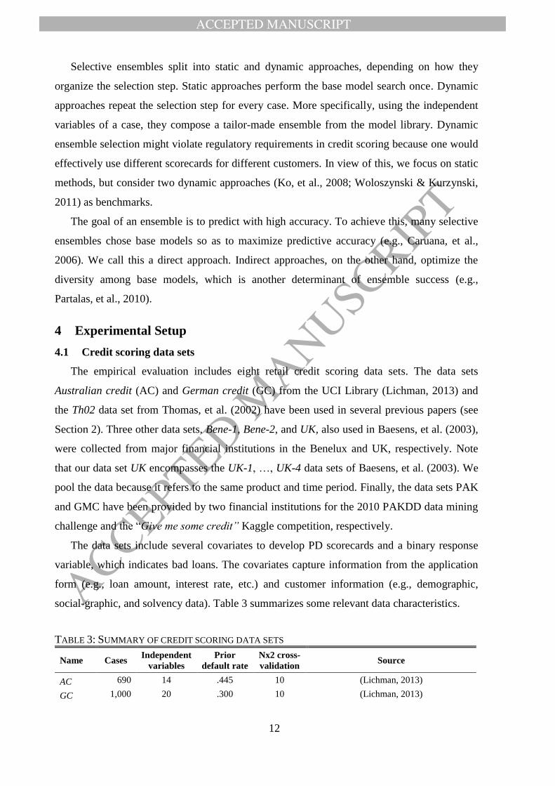
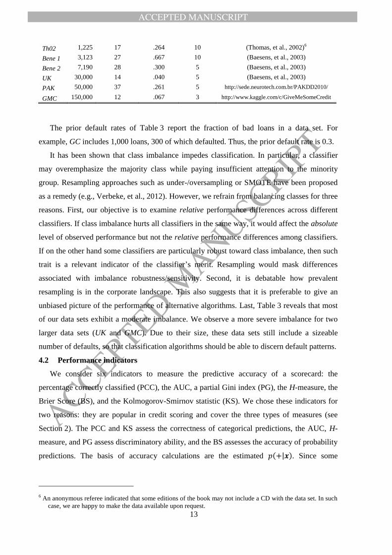
social-graphic, and solvency data). Table 3 summarizes some relevant data characteristics.

TABLE 3: SUMMARY OF CREDIT SCORING DATA SETS

Name Cases Independent

variables

Prior

default rate

Nx2 cross-

validation Source

AC 690 14 .445 10 (Lichman, 2013)

GC 1,000 20 .300 10 (Lichman, 2013)

ACCEPTED MANUSCRIPT

ACCEPTED MANUSCRIP

T

13

Th02 1,225 17 .264 10 (Thomas, et al., 2002)6

Bene 1 3,123 27 .667 10 (Baesens, et al., 2003)

Bene 2 7,190 28 .300 5 (Baesens, et al., 2003)

UK 30,000 14 .040 5 (Baesens, et al., 2003)

PAK 50,000 37 .261 5 http://sede.neurotech.com.br/PAKDD2010/

GMC 150,000 12 .067 3 http://www.kaggle.com/c/GiveMeSomeCredit

The prior default rates of Table 3 report the fraction of bad loans in a data set. For

example, GC includes 1,000 loans, 300 of which defaulted. Thus, the prior default rate is 0.3.

It has been shown that class imbalance impedes classification. In particular, a classifier

may overemphasize the majority class while paying insufficient attention to the minority

group. Resampling approaches such as under-/oversampling or SMOTE have been proposed

as a remedy (e.g., Verbeke, et al., 2012). However, we refrain from balancing classes for three

reasons. First, our objective is to examine relative performance differences across different

classifiers. If class imbalance hurts all classifiers in the same way, it would affect the absolute

level of observed performance but not the relative performance differences among classifiers.

If on the other hand some classifiers are particularly robust toward class imbalance, then such

trait is a relevant indicator of the classifier’s merit. Resampling would mask differences

associated with imbalance robustness/sensitivity. Second, it is debatable how prevalent

resampling is in the corporate landscape. This also suggests that it is preferable to give an

unbiased picture of the performance of alternative algorithms. Last, Table 3 reveals that most

of our data sets exhibit a moderate imbalance. We observe a more severe imbalance for two

larger data sets (UK and GMC). Due to their size, these data sets still include a sizeable

number of defaults, so that classification algorithms should be able to discern default patterns.

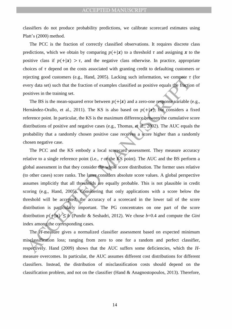
4.2 Performance indicators

We consider six indicators to measure the predictive accuracy of a scorecard: the

percentage correctly classified (PCC), the AUC, a partial Gini index (PG), the H-measure, the

Brier Score (BS), and the Kolmogorov-Smirnov statistic (KS). We chose these indicators for

two reasons: they are popular in credit scoring and cover the three types of measures (see

Section 2). The PCC and KS assess the correctness of categorical predictions, the AUC, H-

measure, and PG assess discriminatory ability, and the BS assesses the accuracy of probability

predictions. The basis of accuracy calculations are the estimated 𝑝(+|𝒙). Since some

6 An anonymous referee indicated that some editions of the book may not include a CD with the data set. In such

case, we are happy to make the data available upon request.

ACCEPTED MANUSCRIPT

ACCEPTED MANUSCRIP

T

14

classifiers do not produce probability predictions, we calibrate scorecard estimates using

Platt’s (2000) method.

The PCC is the fraction of correctly classified observations. It requires discrete class

predictions, which we obtain by comparing 𝑝(+|𝒙) to a threshold 𝜏 and assigning 𝒙 to the

positive class if 𝑝(+|𝒙) > 𝜏, and the negative class otherwise. In practice, appropriate

choices of 𝜏 depend on the costs associated with granting credit to defaulting customers or

rejecting good customers (e.g., Hand, 2005). Lacking such information, we compute 𝜏 (for

every data set) such that the fraction of examples classified as positive equals the fraction of

positives in the training set.

The BS is the mean-squared error between 𝑝(+|𝒙) and a zero-one response variable (e.g.,

Hernández-Orallo, et al., 2011). The KS is also based on 𝑝(+|𝒙), but considers a fixed

reference point. In particular, the KS is the maximum difference between the cumulative score

distributions of positive and negative cases (e.g., Thomas, et al., 2002). The AUC equals the

probability that a randomly chosen positive case receives a score higher than a randomly

chosen negative case.

The PCC and the KS embody a local scorecard assessment. They measure accuracy

relative to a single reference point (i.e., or the KS point). The AUC and the BS perform a

global assessment in that they consider the whole score distribution. The former uses relative

(to other cases) score ranks. The latter considers absolute score values. A global perspective

assumes implicitly that all thresholds are equally probable. This is not plausible in credit

scoring (e.g., Hand, 2005). Considering that only applications with a score below the

threshold will be accepted, the accuracy of a scorecard in the lower tail of the score

distribution is particularly important. The PG concentrates on one part of the score

distribution 𝑝(+|𝒙) ≤ 𝑏 (Pundir & Seshadri, 2012). We chose b=0.4 and compute the Gini

index among the corresponding cases.

The H-measure gives a normalized classifier assessment based on expected minimum

misclassification loss; ranging from zero to one for a random and perfect classifier,

respectively. Hand (2009) shows that the AUC suffers some deficiencies, which the H-

measure overcomes. In particular, the AUC assumes different cost distributions for different

classifiers. Instead, the distribution of misclassification costs should depend on the

classification problem, and not on the classifier (Hand & Anagnostopoulos, 2013). Therefore,

ACCEPTED MANUSCRIPT

ACCEPTED MANUSCRIP

T

15

the H-measure uses a beta-distribution7 to specify the relative severities of classification

errors in a way that is consistent across classifiers.

Given that the class distributions in our data show some imbalance (see Table 3), it is

important to reason whether and how class skew affects the performance measures. The AUC

is not affected by class imbalance (Fawcett, 2006). This feature extends to the other ranking

measures (i.e., the PG and the H-measure) because these ground on the same principles as the

AUC. The BS and the KS are based on the score distribution of a classifier. As such, they are

robust toward class skew in general (e.g., Gong & Huang, 2012). However, class imbalance

could exert an indirect effect in that it might bias the scores that the classifier produces.

Finally, using the PCC in the presence of class imbalance is often discouraged. A common

critic is that PCC reports high performance for naïve classifiers, which always predict the

majority class. However, we argue that this critic is misleading in that it misses the important

role of the classification threshold A proper choice of for example according to Bayes rule,

reflects the prior probabilities of the classes and thereby mitigates the naïve classifier

problem; at least to some extent.

For the reasons outlined above, we consider each of the six performance measures a viable

approach for classifier comparisons. In addition, further protection from class imbalance

biasing the benchmarking results comes from our approach to calibrate predictions prior to

assessing accuracy (see above). Calibration ensures that we compare different classifiers on a

common ground. More specifically, calibration sanitizes a classifier’s score distribution and

thus prevents imbalance from indirectly affecting the BS or the KS. For the PCC, we set

such that the fraction of cases classified as positive is equal to the prior default probability in

the training set. With these strategies in place, we argue that the residual effect of class

imbalance on the observed results comes directly from different algorithms being more or less

sensitive toward imbalance. Such effects are useful to observe as class imbalance is a

common phenomenon in credit scoring.

4.3 Data preprocessing and partitioning

We first impute missing values using a mean/mode replacement for numeric/nominal

attributes. Next, we create two versions of each data set; one which mixes nominal and

numeric variables and one where all nominal variables are converted to numbers using

weight-of-evidence coding (e.g., Thomas, et al., 2002). This is because some classification

algorithms are well suited to work with data of mixed scaling level (e.g., classification trees

7 We use a beta-distribution with parameters 𝛼 = 𝛽 = 2.

ACCEPTED MANUSCRIPT

ACCEPTED MANUSCRIP

T

16

and Bayes classifiers), whereas others (e.g., ANNs and SVMs) benefit from encoding nominal

variables (e.g., Crone, et al., 2006).

An important pre-processing decision concerns data partitioning (see Figure 1). We use

Nx2-fold cross-validation (Dietterich, 1998). This involves i) randomly splitting a data set in

half, ii) using the first and second half for model building and evaluation, respectively, iii)

switching the roles of the two partitions, and iv) repeating the two-fold validation N times.

Compared to using a fixed training and test set, multiple repetitions of two-fold cross-

validation give more robust results, especially when working with small data sets. Thus, we

set N depending on data set size (Table 3). This is also to ensure computational feasibility.

Recall that we develop multiple classification models with one algorithm. The models

differ in terms of their meta-parameter settings (see Table 2). Thus, prior to comparing

different classifiers, we identify the best meta-parameter configuration for each classification

algorithm. This requires auxiliary validation data. We also require validation data to prune

base models in selective ensemble algorithms. To obtain such validation data, we perform an

additional (internal) five-fold cross-validation on every training set of the (outer) Nx2-cross-

validation loop (Caruana, et al., 2006). The classification models selected in this stage enter

the actual benchmark, where we compare the best models from different algorithms in the

outer Nx2 cross-validation loop. Given that model performance depends on the specific

accuracy indicator employed, we repeat the selection of the best model per classifier for every

performance measure. This way, we tune every classifier to the specific performance measure

under consideration and ensure that the algorithm predicts as accurately as possible; given the

predefined candidate settings for meta-parameters (see Table A.1 in the online appendix8).

5 Empirical Results

The empirical results consist of performance estimates of the 41 classifiers across the eight

credit scoring data sets in terms of the six performance measures. Interested readers find these

raw results in Table A.2 – A.7 in the online appendix9. Below, we report aggregated results.

5.1 Benchmarking results

In the core benchmark, we rank classifier performance across data sets and accuracy

indicators. For example, the classifier giving the highest AUC on the AC data sets receives a

rank of one, the second best classifier a rank of two, and the worst classifier a rank of 41.

8 Available at: (URL will be inserted by Elsevier when available)

9 Available online at: (URL will be inserted by Elsevier when available).

ACCEPTED MANUSCRIPT

ACCEPTED MANUSCRIP

T

17

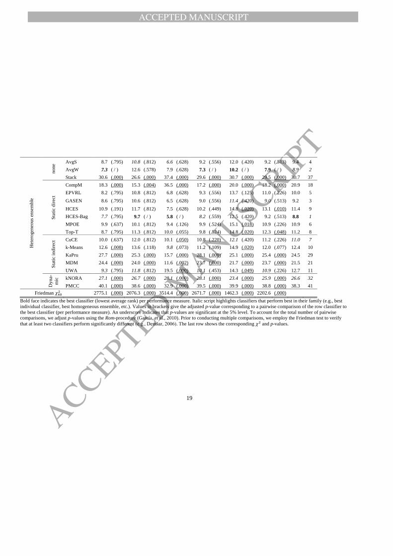
Table 4 shows the average (across data sets) ranks per accuracy indicator. The second to

last column of Table 4 gives a grand average (AvgR), which we compute as the mean

classifier rank across performance measures. The last column translates the AvgR into a high

score position (e.g., the overall best performing classifier receives the first place, the second

best place two, etc.)

The average ranks of Table 4 are also the basis of a statistical analysis of model

performance. In particular, we employ a nonparametric testing framework to compare the

classifiers to a control classifier (Demšar, 2006). The control classifier is the best performing

classifier per performance measure. The last row of Table 4 depicts the test statistic and p-

value (in brackets) of a Friedman test of the null-hypothesis that all classifier ranks are equal.

Given that we can reject the null-hypothesis for all performance measures (p < .000), we

proceed with pairwise comparisons of a classifier to the control classifier using the Rom-

procedure for p-value adjustment (García, et al., 2010). Table 4 depicts the p-values

corresponding to these pairwise comparisons in brackets. An underscore indicates that we can

reject the null-hypothesis of a classifier performing equal to the control classifier (i.e., p <

.05).

A number of conclusions emerge from Table 4. First, it emphasizes the need to update

Baesens, et al. (2003) who focused on individual classifiers. With an average rank of 18.8, the

best individual classifier (ANN) performs only midfield. This evidences notable

advancements in predictive learning since 2003. Similar to Baesens, et al. (2003), we observe

ANN to perform slightly better than the industry standard LR (AvgR 19.3). Some authors

have taken the similarity between LR and advanced methods such as ANN as evidence that

complex classifiers do not offer much advantage over simpler methods (e.g., Finlay, 2009).

We do not agree with this view. Our results suggest that comparisons among individual

classifiers are too narrow to shed light on the value of advanced classifiers. For example, the

p-values of the pairwise comparisons indicate that the individual classifiers predict

significantly less accurately than the best classifier. This shows that advanced methods can

outperform simple classifiers and LR in particular.

ACCEPTED MANUSCRIPT

ACCEPTED MANUSCRIP

T

18

TABLE 4: AVERAGE CLASSIFIER RANKS ACROSS DATA SETS FOR DIFFERENT PERFORMANCE MEASURES

Classifier

family

BM

selection Classifier AUC PCC BS H PG KS AvgR

High

score

Ind

ivid

ual

cla

ssif

ier

n.a

.

ANN 16.2 (.000) 18.6 (.000) 27.5 (.000) 17.9 (.000) 14.9 (.020) 17.6 (.000) 18.8 14

B-Net 27.8 (.000) 26.8 (.000) 20.4 (.000) 28.3 (.000) 23.7 (.000) 26.2 (.000) 25.5 30

CART 36.5 (.000) 32.8 (.000) 35.9 (.000) 36.3 (.000) 25.7 (.000) 34.1 (.000) 33.6 38

ELM 30.1 (.000) 29.8 (.000) 35.9 (.000) 30.6 (.000) 27.0 (.000) 27.9 (.000) 30.2 36

ELM-K 20.6 (.000) 19.9 (.000) 36.8 (.000) 19.0 (.000) 23.0 (.000) 20.6 (.000) 23.3 26

J4.8 36.9 (.000) 34.2 (.000) 34.3 (.000) 35.4 (.000) 35.7 (.000) 32.5 (.000) 34.8 39

k-NN 29.3 (.000) 30.1 (.000) 27.2 (.000) 30.0 (.000) 26.6 (.000) 30.5 (.000) 29.0 34

LDA 21.8 (.000) 20.9 (.000) 16.7 (.000) 20.5 (.000) 24.8 (.000) 21.9 (.000) 21.1 20

LR 20.1 (.000) 19.9 (.000) 13.3 (.000) 19.0 (.000) 23.1 (.000) 20.4 (.000) 19.3 16

LR-R 22.5 (.000) 22.0 (.000) 34.6 (.000) 22.5 (.000) 21.4 (.000) 21.4 (.000) 24.1 28

NB 30.1 (.000) 29.9 (.000) 23.8 (.000) 29.3 (.000) 22.2 (.000) 29.1 (.000) 27.4 33

RbfNN 31.4 (.000) 31.7 (.000) 28.0 (.000) 31.9 (.000) 24.1 (.000) 31.7 (.000) 29.8 35

QDA 27.0 (.000) 26.4 (.000) 22.6 (.000) 26.4 (.000) 23.6 (.000) 27.3 (.000) 25.5 31

SVM-L 21.7 (.000) 23.0 (.000) 31.8 (.000) 22.6 (.000) 19.7 (.000) 21.7 (.000) 23.4 27

SVM-Rbf 20.5 (.000) 22.2 (.000) 31.8 (.000) 22.0 (.000) 21.7 (.000) 21.3 (.000) 23.2 25

VP 37.8 (.000) 36.4 (.000) 31.4 (.000) 37.8 (.000) 34.6 (.000) 37.6 (.000) 35.9 40

Ho

mo

gen

eou

s en

sem

ble

n.a

.

ADT 22.0 (.000) 18.8 (.000) 19.0 (.000) 21.7 (.000) 19.4 (.000) 20.0 (.000) 20.2 17

Bag 25.1 (.000) 22.6 (.000) 18.3 (.000) 23.5 (.000) 25.2 (.000) 24.7 (.000) 23.2 24

BagNN 15.4 (.000) 17.3 (.000) 12.6 (.000) 16.5 (.000) 15.0 (.020) 16.6 (.000) 15.6 13

Boost 16.9 (.000) 16.7 (.000) 25.2 (.000) 18.2 (.000) 19.2 (.000) 18.1 (.000) 19.0 15

LMT 22.9 (.000) 23.4 (.000) 15.6 (.000) 25.1 (.000) 20.1 (.000) 22.9 (.000) 21.7 22

RF 14.7 (.000) 14.3 (.039) 12.6 (.000) 12.8 (.004) 19.4 (.000) 15.3 (.000) 14.8 12

RotFor 22.8 (.000) 21.9 (.000) 23.0 (.000) 21.1 (.000) 21.6 (.000) 22.9 (.000) 22.2 23

SGB 21.0 (.000) 19.9 (.000) 20.8 (.000) 21.2 (.000) 22.5 (.000) 20.8 (.000) 21.0 19

ACCEPTED MANUSCRIPT

ACCEPTED MANUSCRIP

T

19

Het

ero

gen

eou

s en

sem

ble

no

ne

AvgS 8.7 (.795) 10.8 (.812) 6.6 (.628) 9.2 (.556) 12.0 (.420) 9.2 (.513) 9.4 4

AvgW 7.3 ( / ) 12.6 (.578) 7.9 (.628) 7.3 ( / ) 10.2 ( / ) 7.9 ( / ) 8.9 2

Stack 30.6 (.000) 26.6 (.000) 37.4 (.000) 29.6 (.000) 30.7 (.000) 29.5 (.000) 30.7 37

Sta

tic

dir

ect

CompM 18.3 (.000) 15.3 (.004) 36.5 (.000) 17.2 (.000) 20.0 (.000) 18.2 (.000) 20.9 18

EPVRL 8.2 (.795) 10.8 (.812) 6.8 (.628) 9.3 (.556) 13.7 (.125) 11.0 (.226) 10.0 5

GASEN 8.6 (.795) 10.6 (.812) 6.5 (.628) 9.0 (.556) 11.4 (.420) 9.0 (.513) 9.2 3

HCES 10.9 (.191) 11.7 (.812) 7.5 (.628) 10.2 (.449) 14.8 (.020) 13.1 (.010) 11.4 9

HCES-Bag 7.7 (.795) 9.7 ( / ) 5.8 ( / ) 8.2 (.559) 12.5 (.420) 9.2 (.513) 8.8 1

MPOE 9.9 (.637) 10.1 (.812) 9.4 (.126) 9.9 (.524) 15.1 (.018) 10.9 (.226) 10.9 6

Top-T 8.7 (.795) 11.3 (.812) 10.0 (.055) 9.8 (.524) 14.8 (.020) 12.3 (.048) 11.2 8

Sta

tic

ind

irec

t CuCE 10.0 (.637) 12.0 (.812) 10.1 (.050) 10.8 (.220) 12.1 (.420) 11.2 (.226) 11.0 7

k-Means 12.6 (.008) 13.6 (.118) 9.8 (.073) 11.2 (.109) 14.9 (.020) 12.0 (.077) 12.4 10

KaPru 27.7 (.000) 25.3 (.000) 15.7 (.000) 28.1 (.000) 25.1 (.000) 25.4 (.000) 24.5 29

MDM 24.4 (.000) 24.0 (.000) 11.6 (.002) 23.7 (.000) 21.7 (.000) 23.7 (.000) 21.5 21

UWA 9.3 (.795) 11.8 (.812) 19.5 (.000) 10.1 (.453) 14.3 (.049) 10.9 (.226) 12.7 11

Dy

na-

mic

kNORA 27.1 (.000) 26.7 (.000) 28.1 (.000) 28.1 (.000) 23.4 (.000) 25.9 (.000) 26.6 32

PMCC 40.1 (.000) 38.6 (.000) 32.9 (.000) 39.5 (.000) 39.9 (.000) 38.8 (.000) 38.3 41

Friedman 𝜒402

2775.1 (.000) 2076.3 (.000) 3514.4 (.000) 2671.7 (.000) 1462.3 (.000) 2202.6 (.000)

Bold face indicates the best classifier (lowest average rank) per performance measure. Italic script highlights classifiers that perform best in their family (e.g., best

individual classifier, best homogeneous ensemble, etc.). Values in brackets give the adjusted p-value corresponding to a pairwise comparison of the row classifier to

the best classifier (per performance measure). An underscore indicates that p-values are significant at the 5% level. To account for the total number of pairwise

comparisons, we adjust p-values using the Rom-procedure (García, et al., 2010). Prior to conducting multiple comparisons, we employ the Friedman test to verify

that at least two classifiers perform significantly different (e.g., Demšar, 2006). The last row shows the corresponding 𝜒2 and p-values.

ACCEPTED MANUSCRIPT

ACCEPTED MANUSCRIP

T

20

On the other hand, a second result of Table 4 is that sophisticated methods do not

necessarily improve accuracy. More specifically, Table 4 casts doubt on some of the latest

attempts to improve existing algorithms. For example, ELMs and RotFor extend classical

ANNs and the RF classifier, respectively (Guang-Bin, et al., 2006; Rodriguez, et al., 2006).

According to Table 4, neither of the augmented classifiers improves upon its ancestor.

Additional evidence against the merit of sophisticated classifiers comes from the results of

dynamic ensemble selection algorithms. Arguably, dynamic ensembles are the most complex

classifiers in the study. However, no matter what performance measure we consider, they

predict a lot less accurately than simpler alternatives including LR and other well-known

techniques.

Given somewhat contradictory signals as to the value of advanced classifiers, our results

suggest that the complexity and/or recency of a classifier are misleading indicators of its

prediction performance. Instead, there seem to be some specific approaches that work well; at

least for the credit scoring data sets considered here. Identifying these ‘nuggets’ among the

myriad of methods is an important objective and contribution of classifier benchmarks.

In this sense, a third result of Table 4 is that it confirms and extends previous findings of

Finlay (2011). We confirm Finlay (2011) in that we also observe multiple classifier

architectures to predict credit risk with high accuracy. We also extend his study by

considering selective ensemble methods, and find some evidence that such methods are

effective in credit scoring. Overall, heterogeneous ensembles secure the first eleven ranks.

The strongest competitor outside this family is RF with an average rank of 14.8

(corresponding to place 12). RF is often credited as a very strong classifier (e.g., Brown &

Mues, 2012; Kruppa, et al., 2013). We also observe RF to outperform several alternative

methods (including SVMs, ANNs, and boosting). However, a comparison to heterogeneous

ensemble classifiers – not part of previous studies and explicitly requested by Finlay (2011, p.

377) – reveals that such approaches further improve on RF. For example, the p-values in

Table 4 show that RF predicts significantly less accurately than the best classifier.

Finally, Table 4 also facilitates some conclusions related to the relative effectiveness of

different types of heterogeneous ensembles. First, we observe that the very simple approach to

combine all base model predictions through (unweighted) averaging achieves competitive

performance. Overall, the AvgS ensemble gives the fourth-best classifier in the comparison.

Moreover, AvgS predicts never significantly less accurately than the best classifier. Second,

we find some evidence that combining base models using a weighted average (AvgW) might

be even more promising. This approach produces a very strong classifier with second best

ACCEPTED MANUSCRIPT

ACCEPTED MANUSCRIP

T

21

overall performance. Third, we observe mixed results for selective ensemble classifiers.

Direct approaches achieve ranks in the top-10. In many pairwise comparisons, we cannot

reject the null-hypothesis that a direct selective ensemble and the best classifier perform akin.

The overall best classifier in the study, HCES-Bag (Caruana, et al., 2006), also belongs to the

family of direct selective ensembles. Recall that direct approaches select ensemble members

so as to maximize predictive accuracy (see the online appendix for details10

). Consequently,

they compose different ensembles for different performance measures from the same base

model library. In a similar way, using different performance measures leads to different base

model weights in the AvgW ensemble. On the other hand, performance-measure-agnostic

ensemble strategies tend to predict less accurately. Exceptions to this tendency exist, for

example the high performance of AvgS or the relatively poor performance of CompM.

However, Table 4 suggests an overall trend that the ability to account explicitly for an

externally given performance measure is important in credit scoring.

5.2 Comparison of selected scoring techniques

To complement the previous comparison of several classifiers to a control classifier (i.e.,

the best classifier per performance measure), this section examines to what extent four

selected classifiers are statistically different. In particular, we concentrate on LR, ANN, RF,

and HCES-Bag. We select LR for its popularity in credit scoring, and the other three for

performing best in their category (best individual classifier, best homogeneous/heterogeneous

ensemble).

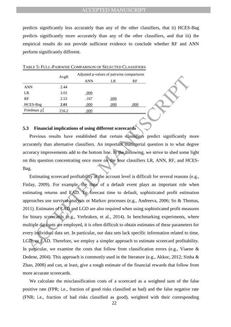
Table 5 reports the results of a full pairwise comparison of these classifiers. The second

column reports their average ranks across data sets and performance measures and the last

row the results of the Friedman test. Based on the observed 𝜒32 = 216.2, we reject the null-

hypothesis that the average ranks are equal (p < .000) and proceed with pairwise comparisons.

For each pair of classifiers, i and j, we compute (Demšar, 2006):

𝑧 = 𝑅𝑖 − 𝑅𝑗 √𝑘(𝑘 + 1)

6𝑁⁄ (1)

where Ri and Rj are the average ranks of classifier i and j, respectively, k (=4) denotes the

number of classifiers, and N (=8) the number of data sets used in the comparison. We convert

the z-values into probabilities using the standard normal distribution and adjust the resulting

p-values for the overall number of comparisons using the Bergmann-Hommel procedure

(García & Herrera, 2008). Based on the results shown in Table 5, we conclude that i) LR

10 Available at: (URL will be inserted by Elsevier when available)

ACCEPTED MANUSCRIPT

ACCEPTED MANUSCRIP

T

22

predicts significantly less accurately than any of the other classifiers, that ii) HCES-Bag

predicts significantly more accurately than any of the other classifiers, and that iii) the

empirical results do not provide sufficient evidence to conclude whether RF and ANN

perform significantly different.

TABLE 5: FULL-PAIRWISE COMPARISON OF SELECTED CLASSIFIERS

AvgR

Adjusted p-values of pairwise comparisons

ANN LR RF

ANN 2.44

LR 3.02 .000

RF 2.53 .167 .000

HCES-Bag 2.01 .000 .000 .000

Friedman 𝜒32 216.2 .000

5.3 Financial implications of using different scorecards

Previous results have established that certain classifiers predict significantly more

accurately than alternative classifiers. An important managerial question is to what degree

accuracy improvements add to the bottom line. In the following, we strive to shed some light

on this question concentrating once more on the four classifiers LR, ANN, RF, and HCES-

Bag.

Estimating scorecard profitability at the account level is difficult for several reasons (e.g.,

Finlay, 2009). For example, the time of a default event plays an important role when

estimating returns and EAD. To forecast time to default, sophisticated profit estimation

approaches use survival analysis or Markov processes (e.g., Andreeva, 2006; So & Thomas,

2011). Estimates of EAD and LGD are also required when using sophisticated profit measures

for binary scorecards (e.g., Verbraken, et al., 2014). In benchmarking experiments, where

multiple data sets are employed, it is often difficult to obtain estimates of these parameters for

every individual data set. In particular, our data sets lack specific information related to time,

LGD, or EAD. Therefore, we employ a simpler approach to estimate scorecard profitability.

In particular, we examine the costs that follow from classification errors (e.g., Viaene &

Dedene, 2004). This approach is commonly used in the literature (e.g., Akkoc, 2012; Sinha &

Zhao, 2008) and can, at least, give a rough estimate of the financial rewards that follow from

more accurate scorecards.

We calculate the misclassification costs of a scorecard as a weighted sum of the false

positive rate (FPR; i.e., fraction of good risks classified as bad) and the false negative rate

(FNR; i.e., fraction of bad risks classified as good), weighted with their corresponding

ACCEPTED MANUSCRIPT

ACCEPTED MANUSCRIP

T

23

decision costs. Let 𝐶(+|−) be the opportunity costs that result from denying credit to a good

risk. Similarly, let 𝐶(−|+) be the costs of granting credit to a bad risk (e.g., net present value

of EAD*LGD – interests paid prior to default). Then, we can calculate the error costs of a

scorecard, C(s), as:

𝐶(𝑠) = 𝐶(+|−) ∗ FPR + 𝐶(−|+) ∗ FNR (2)

Given that a scorecard produces probability estimates 𝑝(+|𝒙), FPR and FNR depend on

the threshold 𝜏. Bayesian decision theory suggests that an optimal threshold depends on the

prior probabilities of good and bad risks and their corresponding misclassification costs (e.g.,

Viaene & Dedene, 2004). To cover different scenarios, we consider 25 cost ratios in the

interval 𝐶(+|−): 𝐶(−|+) = 1: 2, … , 1: 50, always assuming that it is more costly to grant

credit to a bad risk than rejecting a good application (e.g., Thomas, et al., 2002). Note that

fixing 𝐶(+|−) at one does not constrain generality (e.g., Hernández-Orallo, et al., 2011). For

each cost setting and credit scoring data set, we i) compute the misclassification costs of a

scorecard from (2), ii) estimate expected error costs through averaging over data sets, and iii)

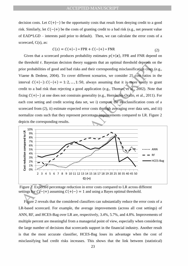
normalize costs such that they represent percentage improvements compared to LR. Figure 2

depicts the corresponding results.

Figure 2: Expected percentage reduction in error costs compared to LR across different

settings for 𝐶(−|+) assuming 𝐶(+|−) = 1 and using a Bayes optimal threshold.

Figure 2 reveals that the considered classifiers can substantially reduce the error costs of a

LR-based scorecard. For example, the average improvements (across all cost settings) of

ANN, RF, and HCES-Bag over LR are, respectively, 3.4%, 5.7%, and 4.8%. Improvements of

multiple percent are meaningful from a managerial point of view, especially when considering

the large number of decisions that scorecards support in the financial industry. Another result

is that the most accurate classifier, HCES-Bag loses its advantage when the cost of

misclassifying bad credit risks increases. This shows that the link between (statistical)

0%

1%

2%

3%

4%

5%

6%

7%

8%

9%

10%

2 3 4 5 6 7 8 9 10 11 12 13 14 15 16 17 18 19 20 25 30 35 40 45 50

Co

st r

ed

uct

ion

co

mp

are

d t

o L

R

C(-|+)

ANN

RF

HCES-Bag

ACCEPTED MANUSCRIPT

ACCEPTED MANUSCRIP

T

24

accuracy and business value is far from perfect. The most accurate classifier does not

necessarily give the most profitable scorecard.

RF and ANN achieve a larger cost reduction than HCES-Bag when misclassifying a bad

risk is eleven and eighteen times more expensive than the opposite error, respectively. Using a

Bayes-optimal threshold, higher costs of misclassifying a bad risk lower the threshold and

thus the acceptance rate. Hence, incorrect rejections of actually good risks become the main

determinant of the error costs of a scorecard. This suggests that the partial superiority of RF

(and ANN) over HCES-Bag results from the latter producing too conservative predictions for

clients with low credit risk. It could be interesting to examine whether this pattern persists if

HCES-Bag were setup to minimize error costs directly (i.e., within ensemble selection). We

leave this test to future research.

5.4 Correspondence of classifier performance across performance measures

Given that many previous studies have used a small number of accuracy indicators, it is

interesting to examine the dependency of observed results on the chosen indicator. Moreover,

such an analysis can add some empirical evidence to the recent debate whether and when the

AUC is a suitable measure to compare different classifiers and retail scorecards in particular

(e.g., Hand & Anagnostopoulos, 2013; Hernández-Orallo, et al., 2011).

Table 6 depicts the agreement of classifier rankings across accuracy indicators using

Kendall’s rank correlation coefficient. With respect to the AUC, we find that empirical results

do not differ much between this measure and the H-measure (correlation: .93). Thus, if a

credit analyst were to choose a scorecard among alternatives, the AUC and the H-measure

would typically give similar recommendations. In fact, Table 6 supports generalizing this

view even further. Pairwise correlations around .90 indicate high similarity between classifier

ranks in terms of the KS and the PCC with those of the AUC and the H-measure. Despite

substantial conceptual differences between these measures (e.g., local versus global

assessment; see Section 4.3), they rank classifiers rather similarly. Therefore, it appears

sufficient to use one of them in empirical classifier comparisons.

A different conclusion emerges for the BS and the PG. Using the same measurement

approach as the AUC, the PG emphasizes the accuracy of a scorecard in the most important

segment of the score distribution. Our results confirm that this captures a different aspect of

performance. For example, the AUC is notably less correlated with the PG than with the H-

measure. However, we observe the smallest correlation between the BS and the other

measures. The BS is the only indicator that assesses the accuracy of probability estimates.

ACCEPTED MANUSCRIPT

ACCEPTED MANUSCRIP

T

25

Table 6 reveals that this notion of performance contributes useful information to a classifier

comparison over and above those captured in the AUC, PCC, H-measure, and KS.

Based on Table 6 we recommend that future studies use at least three performance

measures: the AUC, the PG, and the BS, whereby one could replace the AUC with the H-

measure. The PG and the BS offer an additional angle from which to examine predictive

accuracy. Thus, they should routinely be part of scorecard comparisons.

TABLE 6: CORRELATION OF CLASSIFIER RANKINGS ACROSS PERFORMANCE MEASURES

AUC PCC BS H PG KS

AUC 1.00

PCC .88 1.00

BS .54 .54 1.00

H .93 .91 .56 1.00

PG .79 .72 .51 .76 1.00

KS .92 .89 .54 .91 .79 1.00

6 Conclusions

We set out to update Baesens, et al. (2003) and to explore the relative effectiveness of

alternative classification algorithms in retail credit scoring. To that end, we compared 41

classifiers in terms of six performance measures across eight real-world credit scoring data

sets. Our results suggest that several classifiers predict credit risk significantly more

accurately than the industry standard LR. Especially heterogeneous ensembles classifiers

perform well. We also provide some evidence that more accurate scorecards facilitate sizeable

financial returns. Finally, we show that several common performance measures give similar

signals as to which scorecard is most effective, and recommend the use of two rarely

employed measures that contribute additional information.

Our study consolidates previous work in PD modeling and provides a holistic picture of

the state-of-the-art in predictive modeling for retail scorecard development. This has

implications for academia and industry. From an academic point of view, an important

question is whether efforts into the development of novel scoring techniques are worthwhile.

Our study provides some support but also raises concerns. We find some advanced methods to

perform extremely well on our credit scoring data sets, but never observe the most recent

classifiers to excel. ANNs perform better than ELMs, RF better than RotFor, and dynamic

selective ensembles worse than almost all other classifiers. This may indicate that progress in

the field has stalled (e.g., Hand, 2006), and that the focus of attention should move from PD

ACCEPTED MANUSCRIPT

ACCEPTED MANUSCRIP

T

26

models to other modeling problems in the credit industry including data quality, scorecard

recalibration, variable selection, and LGD/EAD modeling.

On the other hand, we do not expect the desire to develop better, more accurate scorecards

to end any time soon. Likely, future papers will propose novel classifiers and the “search for

the silver bullet” (Thomas, 2010) will continue. An implication of our study is that such

efforts must be accompanied by a rigorous assessment of the proposed method vis-à-vis

challenging benchmarks. In particular, we recommend RF as benchmark against which to

compare new classification algorithms. HCES-Bag might be even more difficult to

outperform, but is not as easily available in standard software. Furthermore, we caution

against the practice to compare a newly proposed classifier to LR (or some other individual

classifier) only, which we still observe in the literature. LR is the industry standard and it is

useful to examine how a new classifier compares to this approach. However, given the state-

of-the-art, outperforming LR can no longer be accepted as a signal of methodological

advancement.

An important question to be answered in future research is whether the characteristics of a

classification algorithm and a data set facilitate appraising the classifier’s suitability for this

data set a priori. We have identified classifiers that work well for PD modeling, but cannot

explain their success. Nonetheless, our benchmark can be seen as a first step toward gaining

explanatory insight in that it provides an empirical fundament for meta-analytic research. For

example, gathering features of individual classifiers and characteristics of the credit scoring

data sets, and using these as covariates in a regression framework to explain classifier

performance (as dependent variable) could help to uncover the underlying drivers of classifier

efficacy in credit scoring.

From a managerial perspective, it is important to reason whether the superior performance

that we observe for some classifiers generalizes to real-world applications, and to what extent

their adoption would increase returns. These questions are much debated in the literature (e.g.,

Finlay, 2011). From this study, we can add some points to the discussion.

First, we show that advancements in computer power, classifier learning, and statistical

testing facilitate rigorous classifier comparisons. This does not guarantee external validity.

Several concerns why laboratory experiments (as this one) may overestimate the advantage of

advanced classifiers remain valid; and might be insurmountable (e.g., Hand, 2006). However,

experimental designs with several cross-validation repetitions, different performance

measures, and appropriate multiple-comparison procedures overcome some limitations of

ACCEPTED MANUSCRIPT

ACCEPTED MANUSCRIP

T

27

previous studies and, thereby, provide stronger support that advanced classifiers have the

potential to increase predictive accuracy not only in the laboratory but also in industry.

Second, our results facilitate some remarks related to the organizational acceptance of

advanced classifiers. In particular, a lack of acceptance can result from concerns that much

expertise is needed to handle such classifiers. Our results show that this is not the case. The

accuracy differences that we observe result from a fully-automatic modeling approach.

Consequently, certain advanced classifiers do not require human intervention to predict

significantly more accurately than simpler alternatives. Furthermore, the current interest in

Big Data indicates a shift toward a data-driven decision making paradigm among managers.

This might further increase the acceptability of advanced scoring methods.

Finally, the business value of more accurate scorecard predictions is a crucial issue. Our

preliminary simulation provides some evidence that the “higher (statistical) accuracy equals

more profit equation” might hold. Furthermore, retail scorecards support a vast number of

business decisions. Consider for example the credit card industry or scoring tasks in online

settings. In such environments, one-time investments (e.g., for hardware, software, and user

training) into a more elaborate scoring technique will pay-off in the long run when small but

significant accuracy improvements are multiplied by hundreds of thousands of scorecard

applications. The difficulties of introducing advanced scoring methods including ensemble

models are more psychological than business related. Using a large number of models, a

significant minority of which give contradictory answers, is counterintuitive to many business

leaders. Such organizations will need to experiment fully before accepting a change from the

historic industry standard procedures.

Regulatory frameworks and organizational acceptance constrain and sometimes prohibit

the use of advanced scoring techniques today; at least for classic credit products. However,

given the current interest in data-centric decision aids and the richness of online-mediated

forms of credit granting, we foresee a bright future for advanced scoring methods in credit

scoring.

References

Abdou, H., Pointon, J., & El-Masry, A. (2008). Neural nets versus conventional techniques in credit scoring in

Egyptian banking. Expert Systems with Applications, 35, 1275-1292.

Abdou, H. A. (2009). Genetic programming for credit scoring: The case of Egyptian public sector banks. Expert

Systems with Applications, 36, 11402-11417.

Abellán, J., & Mantas, C. J. (2014). Improving experimental studies about ensembles of classifiers for

bankruptcy prediction and credit scoring. Expert Systems with Applications, 41, 3825-3830.

Akkoc, S. (2012). An empirical comparison of conventional techniques, neural networks and the three stage

hybrid Adaptive Neuro Fuzzy Inference System (ANFIS) model for credit scoring analysis: The case of

Turkish credit card data. European Journal of Operational Research, 222, 168-178.

ACCEPTED MANUSCRIPT

ACCEPTED MANUSCRIP

T

28

Andreeva, G. (2006). European generic scoring models using survival analysis. Journal of the Operational

Research Society, 57, 1180-1187.

Atish, P. S., & Jerrold, H. M. (2004). Evaluating and tuning predictive data mining models using receiver

operating characteristic curves. Journal of Management Information Systems, 21, 249-280.

Baesens, B., Van Gestel, T., Viaene, S., Stepanova, M., Suykens, J., & Vanthienen, J. (2003). Benchmarking

state-of-the-art classification algorithms for credit scoring. Journal of the Operational Research Society, 54,

627-635.

Bellotti, T., & Crook, J. (2009). Support vector machines for credit scoring and discovery of significant features.

Expert Systems with Applications, 36, 3302–3308.

Breiman, L. (1996). Bagging predictors. Machine Learning, 24, 123-140.

Breiman, L. (2001). Random forests. Machine Learning, 45, 5-32.

Brown, I., & Mues, C. (2012). An experimental comparison of classification algorithms for imbalanced credit

scoring data sets. Expert Systems with Applications, 39, 3446-3453.

Calabrese, R. (2014). Downturn loss given default: Mixture distribution estimation. European Journal of

Operational Research, 237, 271-277.

Caruana, R., Munson, A., & Niculescu-Mizil, A. (2006). Getting the Most Out of Ensemble Selection. In Proc.

of the 6th Intern. Conf. on Data Mining (pp. 828-833). Hong Kong, China: IEEE Computer Society.

Chen, W., Ma, C., & Ma, L. (2009). Mining the customer credit using hybrid support vector machine technique.

Expert Systems with Applications, 36, 7611-7616.

Crone, S. F., Lessmann, S., & Stahlbock, R. (2006). The impact of preprocessing on data mining: An evaluation

of classifier sensitivity in direct marketing. European Journal of Operational Research, 173, 781-800.

Crook, J. N., Edelman, D. B., & Thomas, L. C. (2007). Recent developments in consumer credit risk assessment.

European Journal of Operational Research, 183, 1447-1465.

Demšar, J. (2006). Statistical comparisons of classifiers over multiple data sets. Journal of Machine Learning

Research, 7, 1-30.

Dietterich, T. G. (1998). Approximate statistical tests for comparing supervised classification learning. Neural

Computation, 10, 1895-1923.

Dirick, L., Claeskens, G., & Baesens, B. (2015). An Akaike information criterion for multiple event mixture cure

models. European Journal of Operational Research, 241, 449-457.

Fawcett, T. (2006). An introduction to ROC analysis. Pattern Recognition Letters, 27, 861-874.

Finlay, S. (2009). Credit scoring for profitability objectives. European Journal of Operational Research, 202,

528-537.

Finlay, S. (2011). Multiple classifier architectures and their application to credit risk assessment. European

Journal of Operational Research, 210, 368-378.

Freund, Y., & Schapire, R. E. (1996). Experiments With a New Boosting Algorithm. In L. Saitta (Ed.), Proc. of

the 13th Intern. Conf. on Machine Learning (pp. 148-156). Bari, Italy: Morgan Kaufmann.

Friedman, J. H. (2002). Stochastic gradient boosting. Computational Statistics & Data Analysis, 38, 367-378.

García, S., Fernández, A., Luengo, J., & Herrera, F. (2010). Advanced nonparametric tests for multiple

comparisons in the design of experiments in computational intelligence and data mining: Experimental

analysis of power. Information Sciences, 180, 2044-2064.

García, S., & Herrera, F. (2008). An extension on "Statistical comparisons of classifiers over multiple data sets"

for all pairwise comparisons. Journal of Machine Learning Research, 9, 2677-2694.

Gong, R., & Huang, S. H. (2012). A Kolmogorov–Smirnov statistic based segmentation approach to learning

from imbalanced datasets: With application in property refinance prediction. Expert Systems with Applications,

39, 6192-6200.

Guang-Bin, H., Lei, C., & Chee-Kheong, S. (2006). Universal approximation using incremental constructive

feedforward networks with random hidden nodes. IEEE Transactions on Neural Networks, 17, 879-892.

Hall, M. A. (2000). Correlation-Based Feature Selection for Discrete and Numeric Class Machine Learning. In

P. Langley (Ed.), Proc. of the 17th Intern. Conf. on Machine Learning (pp. 359-366). Stanford, CA, USA:

Morgan Kaufmann

Hand, D. J. (2005). Good practice in retail credit scorecard assessment Journal of the Operational Research

Society, 56, 1109-1117.

Hand, D. J. (2006). Classifier technology and the illusion of progress. Statistical Science, 21, 1-14.

Hand, D. J. (2009). Measuring classifier performance: A coherent alternative to the area under the ROC curve.

Machine Learning, 77, 103-123.

Hand, D. J., & Anagnostopoulos, C. (2013). When is the area under the receiver operating characteristic curve an

appropriate measure of classifier performance? Pattern Recognition Letters, 34, 492-495.

Hand, D. J., & Henley, W. E. (1997). Statistical classification models in consumer credit scoring: A review.

Journal of the Royal Statistical Society: Series A (General), 160, 523-541.

Hand, D. J., Sohn, S. Y., & Kim, Y. (2005). Optimal bipartite scorecards. Expert Systems with Applications, 29,

684-690.

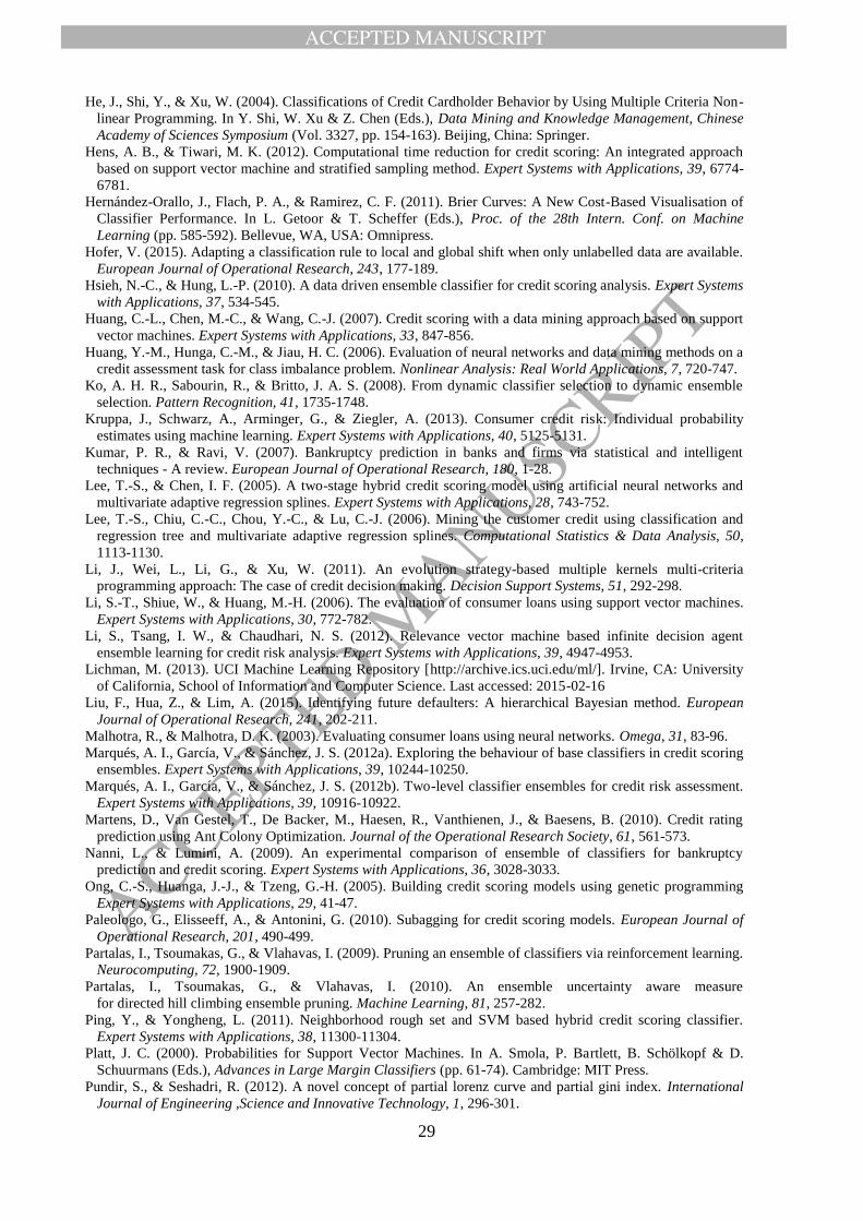
ACCEPTED MANUSCRIPT

ACCEPTED MANUSCRIP

T

29

He, J., Shi, Y., & Xu, W. (2004). Classifications of Credit Cardholder Behavior by Using Multiple Criteria Non-

linear Programming. In Y. Shi, W. Xu & Z. Chen (Eds.), Data Mining and Knowledge Management, Chinese

Academy of Sciences Symposium (Vol. 3327, pp. 154-163). Beijing, China: Springer.

Hens, A. B., & Tiwari, M. K. (2012). Computational time reduction for credit scoring: An integrated approach

based on support vector machine and stratified sampling method. Expert Systems with Applications, 39, 6774-

6781.

Hernández-Orallo, J., Flach, P. A., & Ramirez, C. F. (2011). Brier Curves: A New Cost-Based Visualisation of

Classifier Performance. In L. Getoor & T. Scheffer (Eds.), Proc. of the 28th Intern. Conf. on Machine

Learning (pp. 585-592). Bellevue, WA, USA: Omnipress.

Hofer, V. (2015). Adapting a classification rule to local and global shift when only unlabelled data are available.

European Journal of Operational Research, 243, 177-189.

Hsieh, N.-C., & Hung, L.-P. (2010). A data driven ensemble classifier for credit scoring analysis. Expert Systems

with Applications, 37, 534-545.

Huang, C.-L., Chen, M.-C., & Wang, C.-J. (2007). Credit scoring with a data mining approach based on support

vector machines. Expert Systems with Applications, 33, 847-856.

Huang, Y.-M., Hunga, C.-M., & Jiau, H. C. (2006). Evaluation of neural networks and data mining methods on a

credit assessment task for class imbalance problem. Nonlinear Analysis: Real World Applications, 7, 720-747.

Ko, A. H. R., Sabourin, R., & Britto, J. A. S. (2008). From dynamic classifier selection to dynamic ensemble

selection. Pattern Recognition, 41, 1735-1748.

Kruppa, J., Schwarz, A., Arminger, G., & Ziegler, A. (2013). Consumer credit risk: Individual probability

estimates using machine learning. Expert Systems with Applications, 40, 5125-5131.

Kumar, P. R., & Ravi, V. (2007). Bankruptcy prediction in banks and firms via statistical and intelligent

techniques - A review. European Journal of Operational Research, 180, 1-28.

Lee, T.-S., & Chen, I. F. (2005). A two-stage hybrid credit scoring model using artificial neural networks and

multivariate adaptive regression splines. Expert Systems with Applications, 28, 743-752.

Lee, T.-S., Chiu, C.-C., Chou, Y.-C., & Lu, C.-J. (2006). Mining the customer credit using classification and

regression tree and multivariate adaptive regression splines. Computational Statistics & Data Analysis, 50,

1113-1130.

Li, J., Wei, L., Li, G., & Xu, W. (2011). An evolution strategy-based multiple kernels multi-criteria

programming approach: The case of credit decision making. Decision Support Systems, 51, 292-298.

Li, S.-T., Shiue, W., & Huang, M.-H. (2006). The evaluation of consumer loans using support vector machines.

Expert Systems with Applications, 30, 772-782.

Li, S., Tsang, I. W., & Chaudhari, N. S. (2012). Relevance vector machine based infinite decision agent

ensemble learning for credit risk analysis. Expert Systems with Applications, 39, 4947-4953.

Lichman, M. (2013). UCI Machine Learning Repository [http://archive.ics.uci.edu/ml/]. Irvine, CA: University

of California, School of Information and Computer Science. Last accessed: 2015-02-16

Liu, F., Hua, Z., & Lim, A. (2015). Identifying future defaulters: A hierarchical Bayesian method. European

Journal of Operational Research, 241, 202-211.

Malhotra, R., & Malhotra, D. K. (2003). Evaluating consumer loans using neural networks. Omega, 31, 83-96.

Marqués, A. I., García, V., & Sánchez, J. S. (2012a). Exploring the behaviour of base classifiers in credit scoring

ensembles. Expert Systems with Applications, 39, 10244-10250.

Marqués, A. I., García, V., & Sánchez, J. S. (2012b). Two-level classifier ensembles for credit risk assessment.

Expert Systems with Applications, 39, 10916-10922.

Martens, D., Van Gestel, T., De Backer, M., Haesen, R., Vanthienen, J., & Baesens, B. (2010). Credit rating

prediction using Ant Colony Optimization. Journal of the Operational Research Society, 61, 561-573.

Nanni, L., & Lumini, A. (2009). An experimental comparison of ensemble of classifiers for bankruptcy

prediction and credit scoring. Expert Systems with Applications, 36, 3028-3033.

Ong, C.-S., Huanga, J.-J., & Tzeng, G.-H. (2005). Building credit scoring models using genetic programming

Expert Systems with Applications, 29, 41-47.

Paleologo, G., Elisseeff, A., & Antonini, G. (2010). Subagging for credit scoring models. European Journal of

Operational Research, 201, 490-499.

Partalas, I., Tsoumakas, G., & Vlahavas, I. (2009). Pruning an ensemble of classifiers via reinforcement learning.

Neurocomputing, 72, 1900-1909.

Partalas, I., Tsoumakas, G., & Vlahavas, I. (2010). An ensemble uncertainty aware measure

for directed hill climbing ensemble pruning. Machine Learning, 81, 257-282.

Ping, Y., & Yongheng, L. (2011). Neighborhood rough set and SVM based hybrid credit scoring classifier.

Expert Systems with Applications, 38, 11300-11304.

Platt, J. C. (2000). Probabilities for Support Vector Machines. In A. Smola, P. Bartlett, B. Schölkopf & D.

Schuurmans (Eds.), Advances in Large Margin Classifiers (pp. 61-74). Cambridge: MIT Press.

Pundir, S., & Seshadri, R. (2012). A novel concept of partial lorenz curve and partial gini index. International

Journal of Engineering ,Science and Innovative Technology, 1, 296-301.

ACCEPTED MANUSCRIPT

ACCEPTED MANUSCRIP

T

30

Rodriguez, J. J., Kuncheva, L. I., & Alonso, C. J. (2006). Rotation forest: A new classifier ensemble method.

IEEE Transactions on Pattern Analysis and Machine Intelligence, 28, 1619-1630.

Sinha, A. P., & Zhao, H. (2008). Incorporating domain knowledge into data mining classifiers: An application in

indirect lending. Decision Support Systems, 46, 287-299.

So, M. M. C., & Thomas, L. C. (2011). Modelling the profitability of credit cards by Markov decision processes.

European Journal of Operational Research, 212, 123-130.

Sohn, S. Y., & Ju, Y. H. (2014). Updating a credit-scoring model based on new attributes without realization of

actual data. European Journal of Operational Research, 234, 119-126.

Šušteršič, M., Mramor, D., & Zupan, J. (2009). Consumer credit scoring models with limited data. Expert

Systems with Applications, 36, 4736-4744.

Thomas, L. C. (2010). Consumer finance: Challenges for operational research. Journal of the Operational

Research Society, 61, 41-52.

Thomas, L. C., Edelman, D. B., & Crook, J. N. (2002). Credit Scoring and its Applications. Philadelphia: Siam.

Tong, E. N. C., Mues, C., & Thomas, L. C. (2012). Mixture cure models in credit scoring: if and when borrowers

default. European Journal of Operational Research, 218, 132-139.

Tsai, C.-F. (2014). Combining cluster analysis with classifier ensembles to predict financial distress. Information

Fusion, 16, 46-58.

Tsai, C.-F., & Wu, J.-W. (2008). Using neural network ensembles for bankruptcy prediction and credit scoring.

Expert Systems with Applications, 34, 2639-2649.

Tsai, M.-C., Lin, S.-P., Cheng, C.-C., & Lin, Y.-P. (2009). The consumer loan default predicting model - An

application of DEA-DA and neural network. Expert Systems with Applications, 36, 11682-11690.

Twala, B. (2010). Multiple classifier application to credit risk assessment. Expert Systems with Applications, 37,

3326-3336.

Verbeke, W., Dejaeger, K., Martens, D., Hur, J., & Baesens, B. (2012). New insights into churn prediction in the

telecommunication sector: A profit driven data mining approach. European Journal of Operational Research,

218, 211-229.

Verbraken, T., Bravo, C., Weber, R., & Baesens, B. (2014). Development and application of consumer credit

scoring models using profit-based classification measures. European Journal of Operational Research, 238,

505-513.

Viaene, S., & Dedene, G. (2004). Cost-sensitive learning and decision making revisited. European Journal of

Operational Research, 166, 212-220.

Wang, G., Hao, J., Ma, J., & Jiang, H. (2011). A comparative assessment of ensemble learning for credit scoring.

Expert Systems with Applications, 38, 223-230.

West, D., Dellana, S., & Qian, J. (2005). Neural network ensemble strategies for financial decision applications.

Computers & Operations Research, 32, 2543-2559.

Woloszynski, T., & Kurzynski, M. (2011). A probabilistic model of classifier competence for dynamic ensemble

selection. Pattern Recognition, 44, 2656-2668.

Xiao, W., Zhao, Q., & Fei, Q. (2006). A comparative study of data mining methods in consumer loans credit

scoring management. Journal of Systems Science and Systems Engineering, 15, 419-435.

Xu, X., Zhou, C., & Wang, Z. (2009). Credit scoring algorithm based on link analysis ranking with support

vector machine. Expert Systems with Applications, 36, 2625-2632.

Yang, Y. (2007). Adaptive credit scoring with kernel learning methods. European Journal of Operational

Research, 183, 1521-1536.

Yao, X., Crook, J., & Andreeva, G. (2015). Support vector regression for loss given default modelling. European

Journal of Operational Research, 240, 528-538.

Yap, B. W., Ong, S. H., & Husain, N. H. M. (2011). Using data mining to improve assessment of credit

worthiness via credit scoring models. Expert Systems with Applications, 38, 13274-13283.

Yu, L., Wang, S., & Lai, K. K. (2008). Credit risk assessment with a multistage neural network ensemble

learning approach. Expert Systems with Applications, 34, 1434-1444.

Yu, L., Wang, S., & Lai, K. K. (2009). An intelligent-agent-based fuzzy group decision making model for

financial multicriteria decision support: The case of credit scoring. European Journal of Operational

Research, 195, 942-959.

Yu, L., Yao, X., Wang, S., & Lai, K. K. (2011). Credit risk evaluation using a weighted least squares SVM

classifier with design of experiment for parameter selection. Expert Systems with Applications, 38, 15392-

15399.

Yu, L., Yue, W., Wang, S., & Lai, K. K. (2010). Support vector machine based multiagent ensemble learning for

credit risk evaluation. Expert Systems with Applications, 37, 1351-1360.

Zhang, D., Zhou, X., Leung, S. C. H., & Zheng, J. (2010). Vertical bagging decision trees model for credit

scoring. Expert Systems with Applications, 37, 7838-7843.

Zhang, J., Shi, Y., & Zhang, P. (2009). Several multi-criteria programming methods for classification.

Computers & Operations Research, 36, 823-836.

ACCEPTED MANUSCRIPT

ACCEPTED MANUSCRIP

T

31

Zhou, L., Lai, K. K., & Yu, L. (2010). Least Squares Support Vector Machines ensemble models for credit

scoring. Expert Systems with Applications, 37, 127-133.

ACCEPTED MANUSCRIPT

ACCEPTED MANUSCRIP

T

Classification models1

Validation set predictions

Heterogeneous ensemblealgorithm

Individual classification

algorithm

Homogeneousensemble algorithm

Training set

Validation set

Testset

DataTrain

classifier

Test set prediction

Train ensemble

Ensemble models2

Applymodel

Apply model

Benchmarkclassifier

1 Individual classifier & homogeneous ensemble classifier2 Heterogeneous ensemble classifier

Benchmarking state-of-the-art classification algorithms for credit scoring:

Classification model development and evaluation process