behavioral responses of elk (cervus elaphus) to ) …
TRANSCRIPT
BEHAVIORAL RESPONSES OF ELK (Cervus elaphus) TO
THE THREAT OF WOLF (Canus lupus) PREDATION
by
John Arthur Winnie, Jr.
A dissertation submitted in partial fulfillment of the requirements for the degree
of
Doctor of Philosophy
in
Biological Sciences
Montana State University Bozeman, Montana
April, 2006

© Copyright
by
John Arthur Winnie, Jr.
2006
All rights reserved

ii
APPROVAL
of a dissertation submitted by
John Arthur Winnie, Jr.
This dissertation has been read by each member of the dissertation committee and has been found to be satisfactory regarding content, English usage, format, citations, bibliographic style, and consistency, and is ready for submission to the Division of Graduate Education.
Dr. Scott Creel
Approval for the Department of Ecology
Dr. David Roberts
Approval for the Division of Graduate Education
Dr. Joseph J. Fedock

iii
STATEMENT OF PERMISSION TO USE
In presenting this dissertation in partial fulfillment of the requirements for a
doctoral degree at Montana State University, I agree that the Library shall make it
available to borrowers under rules of the Library. I further agree that copying of
this dissertation is allowable only for scholarly purposes, consistent with “fair use”
as prescribed in the U.S. Copyright Law. Requests for extensive copying or
reproduction of this dissertation should be referred to ProQuest Information and
Learning, 300 North Zeeb Road, Ann Arbor, Michigan 48106, to whom I have
granted “the exclusive right to reproduce and distribute my dissertation in and
from microform along with the non-exclusive right to reproduce and distribute my
abstract in any format in whole or in part.”
John Arthur Winnie, Jr.
April, 2006

iv
TABLE OF CONTENTS
LIST OF TABLES ......................................................................................vi LIST OF FIGURES ...................................................................................vii
1. BEHAVIORAL RESPONSES OF ELK TO THE THREAT OF WOLF
PREDATION: INTRODUCTION ................................................................ 1 2. BEHAVIORAL RESPONSES OF ELK TO THE THREAT OF WOLF
PREDATION: SEX SPECIFIC CONSTRAINTS......................................... 4 Abstract...................................................................................................... 4 Introduction ................................................................................................ 5 Methods ................................................................................................... 11 Study Area .................................................................................... 11 Wolves .......................................................................................... 12 Determining Wolf Presence and Temporal Variation in Predation Risk........................................................................... 12 Elk................................................................................................. 13 Elk Distributions, Herd Sizes and Herd Compositions .................. 14 Elk Behavior.................................................................................. 16 Kill Locations and Carcass Marrow Fat Determination ................. 18 Statistical Methods........................................................................ 19 Results..................................................................................................... 22 Herd Dynamics and Distributions.................................................. 22 Marrow Fat and Predation Risk..................................................... 24 Moving, Bedding and Other Behavior ........................................... 26 Vigilance and Grazing Behavior.................................................... 27 Discussion ............................................................................................... 30
3. RULES FOR HABITAT SELECTION BY ELK ARE SIMPLIFIED BY
THE PRESENCE OF WOLVES............................................................... 39 Abstract ................................................................................................... 39
Introduction.............................................................................................. 40 Methods................................................................................................... 43 Study Area.................................................................................... 43 Elk................................................................................................. 44
Wolves .......................................................................................... 45 Habitat Composition at Elk Locations ........................................... 46

v TABLE OF CONTENTS continued
Environmental Variables ............................................................... 48 Statistical Analysis ........................................................................ 49 Independent Variables .......................................................... 51
Results and Discussion ........................................................................... 53 4. SUMMARY AND SOME CAVEATS ............................................................... 61 Summary ................................................................................................. 61 Trophic Cascades.................................................................................... 63 Influences of indirect Costs on Prey Population Dynamics..................... 66 REFERENCES CITED ....................................................................................... 68 APPENDIX A: Model Parameters in Best Models .............................................. 76

vi
LIST OF TABLES Table Page 1.1. Herd size changes in relation to wolf presence .......................................... 24 1.2 Associations between elk behavior and sex, location, position within herd,
and wolf presence. Part b presents an analysis separate from the main factorial ANOVA, addressing the effects of distance to timber .................. 27 2.1. Habitat attributes of elk GPS locations with wolves present and absent, and global model goodness-of-fit.............................................................. 54 2.2. Coefficients and their standard errors from model averaging using AICc weights (ωi). ............................................................................................... 57 2.3. Relative importance values from AICc........................................................ 57

vii
LIST OF FIGURES
Figure Page 1.1. Effect of wolf presence on the distance between elk herds and woodland edges (protective cover)........................................................... 23 1.2. Sex differences and winter changes in physical condition, as measured by femur marrow fat concentration. ........................................ 25 1.3 . Vigilance differences between the sexes in behavioral responses to the presence of wolves. ................................................................................. 29 1.4. Grazing differences between the sexes in behavioral responses to the presence of wolves. ................................................................................. 29 2.1 Summary of the best models of habitat selection by elk............................. 56
1
CHAPTER 1
BEHAVIORAL RESPONSES OF ELK TO THE THREAT OF WOLF PREDATION
Introduction
The effects of predators on prey population dynamics have traditionally
been viewed, and modeled, as direct offtake (Lotka 1925; Bergerud and Elliot
1986, 1998; Berryman 1992; Boyce 1993; Hayes and Harestad 2000). However,
prey respond to the mere threat of predation risk and these responses carry
costs (Morgantini & Hudson 1979, 1985; Werner et al. 1983; Lima and Dill 1990;
Illius and Fitzgibbon 1994; Abramsky et al. 1996). Prey responses to predation
threat range from shifts in habitat use with associated reductions in food quality
or quantity (Morgantini & Hudson 1979, 1985; Heithaus & Dill 2002), to changes
in individual and grouping behaviors that reduce feeding rates or locally increase
intraspecific competition for food (Elgar 1989; Roberts 1996).
Because most prey (not just those individuals about to be killed by
predators) respond to the threat of predation, the costs of risk reduction are likely
to manifest themselves at both the individual and the population level, and may
even exceed direct offtake (Ives and Dobson 1987; Bolnick and Preisser 2005).
Differences between individual prey in behavioral responses that can be
attributed to differences in physiological constraints will give an indication of the
costs associated with antipredator behaviors. If these costs are sufficiently large

2
in terrestrial vertebrates, then efforts should be made to incorporate them into
future models of predator-prey interactions. The following work addresses elk
behavioral responses to the threat of wolf predation, responses that are likely to
carry costs, and singly or in concert, manifest themselves through changes in elk
population dynamics.
Each of the two main sections are papers currently in review, and both are
continuations of work already published (Creel and Winnie 2005, Creel et al
2005). There is some overlap in the introductions and methods sections and
each section has its own abstract. Because of this, the main sections (chapters
2 and 3) can be read as stand-alone works, or viewed as part of the larger body
of work.
The first main section, Sex-specific behavioral responses of elk to spatial
and temporal variation in the threat of wolf predation, addresses elk anti-predator
behavior at the scale of individual behaviors (time budgets), and landscapes
(distribution within a drainage). We found sex specific behavioral responses to
threat that appear to be constrained by body condition, implying that antipredator
behaviors carry caloric costs. In addition to these results, the dichotomy between
cow and bull behavior lends insights into the mechanisms driving sexual
segregation in elk, and here we propose a simple explanation for this
phenomenon.
The second main section, Rules for Habitat Selection by Elk are Simplified
by the Presence of Wolves, compares elk decision making processes during high
versus low risk periods. Although this chapter addresses habitat use decisions, it

3
does not directly deal with landscape level issues. Rather, it investigates the
environmental variables that elk respond to when making habitat use decisions.
The results from this section point to constraints on the elk decision making
process that possibly reducing elk foraging and movement efficiency when
wolves are present in a drainage. As such, this section addresses subtle, and
heretofore undressed, costs associated with predator avoidance.
Throughout a manuscript I use the term “we” because the work involved
extensive collaboration between myself, my advisor Dr. Scott Creel, fellow
graduate student David Christianson, and Dr. Bruce Maxwell and his students
and lab personnel in the LRES department at Montana State University.

4
CHAPTER 2
SEX-SPECIFIC BEHAVIORAL RESPONSES OF ELK TO SPATIAL AND TEMPORAL VARIATION IN THE THREAT OF WOLF PREDATION
Abstract
We studied individual and herd level behavioral responses of elk to spatial
and temporal variation in the risk of predation by wolves over three winters in the
Upper Gallatin drainage, Montana. Within a given drainage, elk of both sexes
moved into or closer to protective cover (timber) in response to wolf presence.
Cow elk responded to elevated risk by increasing vigilance in exchange for
foraging, and large mixed (cow, calf, spike) herds substantially decreased in size.
In contrast, when wolves were present, bulls did not increase vigilance levels, nor
decrease feeding, and small bull-only groups slightly increased in size. As a
consequence, small bull-only herds and large mixed sex herds converged on a
similar size when wolves were present. We believe this response is a balancing
of the benefits of risk dilution with increased detectability or attractiveness of
larger herds to wolves. Based on proportions in the population, wolves
overselected bulls and underselected cows as prey. Thus, bulls showed weaker
antipredator responses than cows, despite facing a greater risk of predation.
Using marrow fat content from elk killed by wolves as an indicator of body
condition, bulls were in significantly worse body condition than cows throughout
the winter, and condition deteriorated for both sexes as winter progressed.

5
Overall, we conclude that: anti-predator behaviors carry substantial foraging
costs; bulls, due to their poorer body condition, are less able to pay these costs
than cows; and differences in ability to pay foraging costs likely explain sex
specific differences in anti-predator behaviors.
Introduction
Anti-predator behavior is well documented across a wide variety of taxa, at
many spatial and temporal scales. At relatively broad scales, prey often alter
their use of habitats in response to predation risk, trading security for a reduction
in forage quality, quantity, or both. Bottlenose dolphins (Tursiops aduncus) avoid
shallow, productive foraging areas during seasons when tiger sharks
(Galeocurdo cuvier) are present, but favor these areas when sharks are absent
(Heithaus & Dill 2002). Elk (Cervus elaphus) move out of open grassy habitats
into less nutritionally profitable closed, forested habitats during human hunting
seasons (Morgantini & Hudson 1985). When faced with the threat of predation
by trained barn owls (Tyto alba), desert gerbils (Gerbillus allenbyi and G.
pyramidum) limit their foraging activity and avoid open areas, foraging under
cover in brushy habitats (Abramsky et al. 1996). In experimental studies, the
presence of predatory large mouth bass (Micropterus salmoides) limited small
bluegill sunfish (Lepomis macrochirus) to vegetated habitats near shore,
significantly reducing their growth rate (Werner et al. 1983).
At finer temporal and spatial scales, prey often alter their behavior in
response to changes in predation risk. Among the most studied of these

6
responses are changes in vigilance levels, group formation, and interactions
between the two (Elgar 1989; Lima & Dill 1990; Roberts 1996). Individuals may
increase vigilance in response to elevated threat, and as with habitat shifts, this
response often carries a foraging cost, typically paid with a reduction in foraging
time (Jennings & Evans 1980; Underwood 1982; Berger & Cunningham 1988;
Lima 1998; Abramsky et al. 2002).
Prey may benefit by grouping through multiple mechanisms, which may
interact: collective vigilance (Pulliam 1973; Powell 1974; Kenward 1978; Roberts,
1996); confusion of attacking predators or cooperative defense (Cresswell 1994;
Krause & Godin 1995); dilution of individual risk (Lima & Dill 1990; Cresswell
1994); and attack abatement (Turner & Pitcher 1986; Uetz & Hieber 1994).
Individual vigilance levels often decline with increasing group size, which implies
that prey do indeed perceive themselves as safer in larger groups (Roberts 1996;
but see Elgar 1989, for a critical review).
The benefits of grouping are reduced (and potentially reversed) if
predators can detect large groups more easily, or prefer to attack them. Several
authors have reported that larger groups are more often detected and attacked,
but some have shown that despite this - and sometimes despite higher predator
success when attacking large groups - individual prey in larger groups are still
safer, due to offsetting benefits of dilution (Creel & Creel 2002; Hebblewhite &
Pletscher 2002), collective detection or cooperation in escape (Krause & Godin
1995), or combinations of these effects (Cresswell 1994; Uetz & Hieber 1994).

7
Predation risk varies in space and time. In the absence of constraints,
prey would respond to risk and minimize predation rates in all places at all times.
However, anti-predator behaviors commonly carry foraging costs (Lima & Dill
1990; Lima,1998), and when prey must exchange food for security, constraints
on both foraging and antipredator behaviors are inevitable. Constraints vary
among individuals depending on nutritional status, and vulnerability to predation
should similarly vary (Lima & Dill 1990; Sinclair & Arcese 1995; Lima 1998).
Consequently, an individual’s physical condition is likely to affect its behavioral
response to variation in risk. Nutritionally compromised individuals should be
less responsive if they are unable to pay the costs associated with reducing
predation risk (Bachman 1993; Lima 1996). Notably, despite the widespread
assumption that elevated vigilance confers greater security, few studies have
directly shown higher predator attack rates upon, or higher mortality rates for,
individuals displaying lower vigilance (but see Fitzgibbon 1988, 1990; and Scheel
1993 for a comparison of species).
Differences in behavioral responses that can be attributed to differences in
physiological constraints will give an indication of the costs associated with
antipredator behaviors. Because most prey (not just those individuals about to
be killed by predators) respond to the threat of predation, the costs of risk
reduction are likely to manifest themselves at both the individual and the
population level, and may even exceed direct offtake (Ives and Dobson 1987;
Bolnick and Preisser 2005). If these costs are sufficiently large in terrestrial

8
vertebrates, then efforts should be made to incorporate them into future models
of predator-prey interactions.
We know of no field studies that have attempted to directly assess
behavioral responses of prey to interactions between body condition, spatial
variation in risk, and temporal variation in risk. This is particularly true for studies
in which true predation risk varied naturally across space and through time,
rather than using simulated risk or experimentally controlled predation. Here we
examine the vigilance, grouping and cover seeking responses of elk (Cervus
elaphus) to fine scale variations in both spatial (distance to protective cover
[timbered areas], position in herd) and temporal (wolf [Canis lupus] presence)
risk, and further ask how these behaviors are constrained by prey physical
condition.
Because it was not possible to sample physical condition for the general
elk population, we compared the behavior of two classes that prior research
indicates are under different energetic constraints through winter: bulls (branch
antlered males with brow tines) and cows (females > 1 year old). Bull elk enter
winter weakened by the fall rut, having lost as much as 20% of their pre-rut
(August) body mass by mid-November, and continue to lose weight more rapidly
than cows throughout the winter (Anderson et al. 1972; Mitchell et al. 1976; Geist
2002; Hudson et al. 2002). In contrast, cow elk typically lose less than 10% of
their body mass between August and May, ending most winters with
proportionally less weight loss than bulls experience prior to winter’s onset. It
should be noted that in most populations over 80% of cows are pregnant each

9
winter, and a cow’s spring weight includes that of her developing fetus - so most
cows’ personal over winter weight losses are greater than 10%. However, fetus
growth is approximately exponential, with the majority of fetal weight gain
occurring in the spring, so cow weight loss is typically low for most of winter
(Hudson et al. 2002; Geist 2002; Cook et al. 2004). Here we attempt to confirm
differences in body condition by comparing the bone marrow of wolf-killed bulls
and wolf-killed cows. The chief limitation to this approach is that wolf-killed elk
do not represent a random sample of the population at large. We do not assume
in our analyses that marrow fat is the same in the sample of killed animals as in
the general population. We do assume that any differences in condition between
live elk and wolf killed elk are the same for males and females. In other words,
the data force an assumption that loss of body condition would increase the risk
of predation in the same manner for cows and bulls.
We tested the hypotheses that:
1. Vigilance levels for elk would increase when wolves were present, for both
sexes (i.e. elk are sensitive to short term temporal variation in risk).
2. Vigilance would decrease with increasing group size (assuming that elk find
greater security in larger groups).
3. Vigilance would increase with distance to timber (i.e. elk are sensitive to fine-
scale spatial variation in risk). Here we assume that elk perceive timber as
protective cover, because we have previously used the distribution of kill sites
to show that risk increases with distance to timber (Creel & Winnie 2005).

10
4. Vigilance is higher on the periphery of herds since these animals might be the
first to encounter attacking wolves (Jennings & Evans 1980; Berger &
Cunningham 1988; Fitzgibbon 1990).
5A. Bulls in our study area would display a greater increase in vigilance than
cows when wolves were present. Several studies of wolf-ungulate
interactions have found that males are preferentially selected by wolves in
winter (Kolenosky 1972; Huggard 1993; Mech et al. 2001). Our evaluation of
this hypothesis includes testing whether or not bulls are preferentially preyed
upon in this population. For this hypothesis we assume variation in risk is
the primary driver of variation in vigilance in elk.
5B. In direct opposition to hypothesis 5A, bulls would show a smaller increase in
vigilance if they were in poorer condition than cows, when wolves were
present. Our evaluation of this hypothesis includes testing whether bulls are
in poorer condition than cows in this population. For this hypothesis we
assume that variation in constraints is the primary driver of variation in
vigilance in elk.
Evaluating hypotheses 5A and 5B constitutes a test of the relative
strengths of predation risk and foraging costs, in their effects on elk behavior. A
priori, it is difficult to know whether variation in antipredator responses will be
more closely associated with variation in risk, or with variation in the costs of
response. Logic cannot resolve this question: it must be addressed empirically.
11
Methods
Study Area
Our study area covers 125.8 km2 in four drainages along the upper
Gallatin River (Porcupine [30.3 km2], Taylor [56.0 km2], Tepee [13.1 km2] and
Daly [26.4 km2]), on a combination of National Forest, National Park, State, and
private land. South-facing slopes and valley bottoms are generally a mixture of
open sage (Artemesia spp.) and grassland (dominated by Idaho fescue Festuca
idahoensis and bluebunch wheatgrass Agropyron spicatum) with riparian areas
bordering small creeks and the upper Gallatin River. North-facing slopes and
higher elevations are primarily coniferous forest (lodgepole pine and Douglas fir:
Pinus contorta & Pseudotsuga menziessii) broken by occasional small meadows.
Elevation runs from 1975 m to 2432 m above sea level.
Two properties of the upper Gallatin drainage provided good conditions
with which to test our hypotheses. First, a short growing season and harsh
winters mean that elk face energetically difficult conditions that produce notable
differences between cows and bulls during the winter study season (see
Results). Second, wolves enter and leave each of the four drainages many times
per winter, creating substantial variation in predation pressure within and among
drainages.

12
The data analyzed here were collected during periods that elk were on
their winter range, beginning around January 1 each year and ending at melt out
in late May or early June over three winters (2001 - 2003).
Wolves
Wolves colonized the study area in 1997. During the study, we had 1, 3,
and 2 packs per year using the study area. The total number of wolves using the
study area each year ranged from 12 to16. The Chief Joseph pack’s territory
overlapped most of the Tepee, Daly and Taylor drainages, plus extensive areas
inside Yellowstone National Park that were outside of the study area. Frequent
movements of the Chief Joseph pack on and off the study site produced
substantial short-term variation in predation risk. This pack held 12, 7 and 12
wolves in the winters of 2000-01, 2001-02 and 2002-03, respectively and denned
in the Daly Creek drainage each spring. Two smaller packs attempted to den in
the study area, one in Porcupine (2001), which apparently failed, and the other in
the Taylor Fork drainage (2002 and 2003). The Taylor Fork wolves (Sentinel
pack) successfully bred both years, producing ≥3 pups both years.
Determining Wolf Presence and Temporal Variation in Predation Risk
While walking fixed transect routes, and during daily visits to drainages,
we continuously checked for signs that wolves were present within a drainage on
that day. We considered wolves present within a drainage if we located them via
VHF radiotelemetry, found a fresh kill, fresh scat, or fresh tracks in snow, mud or

13
loose soil. The number of radiocollared wolves in the study area varied within
and between years due to mortality and dispersal. In the Chief Joseph pack, 0-6
wolves carried radiocollars. In the Sentinel pack, 0-2 carried radiocollars, and no
wolves were collared in the short-lived pack in the Porcupine drainage. If wolves
denned in a drainage (typically near April 15th), we scored all days during the
denning period as having wolves present. Because not all wolves in the study
area were radiocollared and we undoubtedly missed some physical evidence of
their presence, it is likely that we failed to detect wolves on some days. This
classification is conservative – failure to detect wolf presence might mask
responses by elk to wolves (Type II errors), but should not create apparent
differences where none exist (Type I errors).
Elk
Elk in the study area are part of a seasonally migratory population
(averaging 1725 ± 63 SE: minimum and maximum counts of 1214 and 3028
since 1928) that winters along the tributaries of the upper Gallatin River from the
northwest corner of Yellowstone National Park, north to Big Sky, Montana.
Summer range for most of the population is at higher elevations within western
Yellowstone National Park. The migration route and winter range have changed
little over the past 75 years (Brazda 1953; Peek et al. 1967; Peek & Lovaas
1968; Winnie & Creel unpublished data).

14
Most elk herds were small (mean = 13.9 ± 0.67 SE, max = 253 elk: ground
counts of 1143 herds in winter) and concentrated in the four study area
drainages, avoiding the steep, rocky terrain typical of the rest of the region.
Based on VHF radio telemetry and GPS telemetry data, elk rarely moved
between drainages during the study period (20,400 fixes from 47 individuals over
2 years).
Moose (Alces alces), mule deer (Odocoileus hemionus) and white tailed
deer (Odocoileus virginianus) were present in the study area at low densities.
Elk comprised more than 90% of our ungulate observations, and more than 90%
of wolf kills we detected were elk (Creel & Winnie 2005).
Elk Distributions, Herd Sizes and Herd Compositions
Within every two-week interval from mid- January until the end of May, we
surveyed fixed areas (viewsheds) in each of the four drainages, beginning at first
light. Survey routes were chosen to maximize the area scanned in each
drainage while minimizing disturbance caused by our presence. During a survey
we scanned from fixed highpoints, using a tripod mounted 40-56X Nikon ED
spotting scope, and used 10X binoculars while moving between highpoints.
Each drainage was divided into 6-8 fixed zones, based upon viewsheds. Even
though these are not comprehensive counts of all elk within a drainage, we refer
to these bi-weekly counts as censuses. In addition to this formal sampling
regimen, we attempted to visit each drainage on every day of the winter-spring
study period, in either the morning or evening, usually traversing part of our fixed
15
sampling routes. These ad-lib samples provided additional information on herd
sizes and compositions, and wolf presence.
Upon sighting elk we noted the following: UTM location; herd size;
composition (calves [young of the year, either sex], bulls [adult males with brow
tines], cows [females > 1 year old], spikes [one year-old antlered males with no
brow tine and usually no branching], and unknown); distance to timber in four
classes (0-30 m, 31-100 m, 101-300 m, and 301+ m); primary activity (vigilant,
grazing, moving, bedded, other); and habitat type (timber, grass, riparian, sage,
combinations, other). Over three winters, we recorded these data for 1143 elk
herds.
We regularly checked among observers (three individuals) for agreement
on calf classification and our assessments were consistent. Our criteria as to
what constituted separate herds were also tested and consistent. Rather than
apply a simple rule to define herd membership (i.e. all elk within 5 body lengths
of each other comprise a herd), we chose to let elk behavior define herds. Early
in the study, we made preliminary observations and developed the following
criteria to define herds as groups that behave as discrete units: inter-elk spacing
tends to be consistent within herds; individuals tend to be oriented and moving in
the same direction; individuals tend to move at the same speed within herds or to
be simultaneously stationary; and large gaps that well exceeded intra-group
spacing defined separate groups. Using this definition, most herds of 2 or more
elk (732 out of 992) had mean intra-group spacing of 5 body lengths or less.
Small, widely scattered herds typify the Gallatin population (mean herd size =
16
13.9 elk, SE = 0.67, maximum = 253; median distance between observed herds
= 1.40 km, mean = 1.66 km, SE = 47.5 m) – inter-herd distances were two to
three orders of magnitude greater than intra-herd spacing for most (74%) herds.
In our demographic classifications, we did not combine spikes (yearling
males) with bulls, because of important behavioral and physiological differences.
Bulls often segregate themselves from cow-calf herds, while spikes usually do
not. Spikes rarely breed, and consequently avoid the energetic costs of rutting
and concomitant survival costs later in the winter (Geist 2002). We did not
distinguish yearling cows from older cows. Yearling cows often breed, placing
them under similar energetic constraints to older cows (Cook et al., 2004).
Moreover, we could not reliably distinguish yearlings and older cows under field
conditions.
We estimated herd distances to timber in the field using a combination of
GPS fixes and USGS topographic maps rather than using GIS, because ground
truthing of US Forest Service raster maps of habitat types revealed that locations
of habitat edges were often not accurate.
Elk Behavior We gathered behavioral data in every two-week period in each of the 4
drainages from mid-January to the end of May, in 2002 and 2003. To avoid
affecting the animals’ behavior, we made observations at distances of
approximately 0.5 to 2 km through spotting scopes or binoculars. If a herd
retreated from observers or showed other signs of being affected by our
17
presence (such as vigilance directed towards us), or if it became apparent that
we were mis-classifying the herd due to terrain features that hid some individuals
from us for part of the session, we stopped observations and discarded the entire
session’s data. In addition to the following behavioral data, we recorded all of the
data described above in Elk Distributions, Herd Sizes and Compositions.
We used instantaneous scan sampling, which provides an accurate and
unbiased measure of the proportion of time spent engaged in each behavior
(Altmann 1974; Hanson et al. 1993; MacDonald et al. 2000). At five minute
interval, for a minimum of six and a maximum of 13 intervals, we scanned
through herds noting: sex and age (cow, calf, bull, spike, unknown); position
within the herd (peripheral or interior); and behavior (grazing, moving, vigilant,
bedded, other) of every animal in the herd.
We defined interior animals as those that a predator from outside the herd
could not approach without first encountering another herd member. Peripheral
animals were those individuals that could first be encountered by a predator that
approached from outside the herd. We classified a set of mutually exclusive
behaviors as follows: Grazing animals were those standing with their heads down
in forage or a hoofed-out crater in snow; Moving animals were either walking or
running; Vigilant animals were standing or bedded (see note below), head erect,
with ears cocked forward in the direction of gaze; Bedded animals were lying
down, often ruminating, and rarely, sleeping; Other includes relatively infrequent
behaviors such as grooming or sparring. We collected behavioral data on 88
herds, and logged 11,287 instantaneous individual behaviors. A note regarding

18
vigilance: As with many African ungulates (Underwood 1982), elk vigilance is
performed to the exclusion of foraging – even if an elk has a mouth full of food, it
normally stops chewing while vigilant. Moreover, elk feeding behavior is not
limited to grazing and browsing, but also includes extended periods of rumination
that are essential and often performed while bedded (Cook 2002). Because time
spent vigilant while bedded interrupts rumination, it is likely to carry nutritional
costs, so we pooled animals that were vigilant while bedded with other vigilant
animals.
Kill Locations and Carcass Marrow Fat Determination We located wolf kills using a combination of techniques: scanning for
signs of wolf chases and kill sites from transects and high points; backtracking
wolves through snow; following or scanning for scavengers (ravens, eagles,
magpies and coyotes); and investigating sites where wolves congregated for
more than a few hours (usually determined using VHF telemetry). Upon finding a
carcass, we recorded the same information as described above for live elk
observations. We also examined the carcass to determine the likely cause of
death, estimated when death occurred, extracted an incisor for aging using
dental cementum annuli (Matson Labs, Milltown, Montana), and cut an
approximately 8 cm section from the middle of a femur to obtain a marrow
sample. Marrow fat is a commonly used indicator of body condition in ungulates.
This is the last fat reserve tapped by ungulates, and substantial declines in

19
percent fat indicate an animal is, or has been, operating at a caloric deficit
(Neiland 1970; Sinclair & Arcese 1995).
We stored the femur sections in sealed plastic bags in a deep freezer
until analysis the following summer. We used a Soxhlet extractor and the
method described by Neiland (1970) to extract and determine percent marrow fat
of wet weight, with one modification: we exchanged the solvent until the samples
stopped losing weight (some of the samples with higher proportions of fat
required 4 solvent changes before all fat was removed). Out of 59 definite and
probable wolf kills, 33 provided marrow samples from animals that we could
determine were bulls or cows (bulls, n=23; cows, n=10).
Statistical Methods
The dependent variables in our analyses of behavior were total proportion
of time spent vigilant, grazing, moving, bedded, and other. We arcsin-
transformed these proportions to obtain normality (Zar, 1999). All independent
variables were categorical: wolf presence, sex, herd position, and distance to
timber.
We hypothesized a priori that sex, wolf presence, herd position, and
distance to timber might affect vigilance through main effects or interactions.
However, distance to timber was not significantly associated with vigilance as a
main effect or in any interactions in exploratory analysis. Because of this result
(which is somewhat surprising and discussed later), we used information content
(AICc) to determine which independent variables to include in our primary

20
analyses (Burnham and Anderson 2002, Stephens et al. 2005). Based on AICc,
the best model included wolf presence, sex, and position in herd. A model with
these effects and distance to timber was 3.5 AICc units worse. Therefore, we
removed distance to timber from our primary analyses and used fixed effect
factorial ANOVA. We tested for differences in behavioral responses between the
four drainages and found none, so we pooled the data across drainages.
We addressed potential pseudoreplication in three ways. First, our basic
unit of observation was the herd. Elk herd sizes and compositions changed
frequently on our study site, relative to the two-week interval at which we
recorded behavioral observations (as also reported by Shoesmith, [1980] in his
study of 236 marked elk on Yellowstone’s Mirror Plateau). Consequently, it was
not possible to make repeated observations on specific herds: a set of individuals
that formed a herd at one time were very unlikely to be aggregated in the same
way during the next two week interval. Consequently, we considered each herd
a unique observation and the degrees of freedom for ANOVA were based on the
number of herds observed. Second, repeated scans within one observation
period produced a single data point. That is, we pooled across individuals and
scans within each herd to derive a single proportion of time spent in each
behavior for each of the age by sex by position classes in each herd observed.
Finally, we evaluated our assumption that the behavior of different age-sex
classes was functionally independent in our data set. Of the 88 herds we
observed, only 14 (16%) held both cows and bulls. Sexual segregation is
common among ungulates (Clutton-Brock et al. 1987; Main & Coblentz 1990).

21
Of the 14 mixed-sex herds, 6 (6.8%) occurred when wolves were present, and 8
(9%) when wolves were absent, with moderate positive (but not significant at α =
0.05) correlations between cow and bull vigilance in both cases (r2=0.393, P =
0.183, & r2 = 0.17, P = 0.309, respectively). Also, if positive correlations exist in
mixed herds, they will tend to mask differences between bull and cow behavior,
creating conservative, Type 2 errors. Given these patterns, we pooled the 14
integrated herds with the 74 segregated herds. For the purposes of our
analyses, the main point is that 84% of behavioral observations came from
single-sex herds, so that correlations between the behaviors of bulls and cows
have relatively little effect.
To test whether vigilance levels respond to herd size, we used simple
linear regression, using arcsin transformed proportion of vigilance (Zar, 1999), as
the dependent variable and herd size as the independent variable.
We used contingency tables (Zar 1999) to test whether the presence of
wolves affected the number of herds (and individuals) seen at various distances
to timber.
The dependent variable in our marrow fat analysis was proportion fat, and
the independent variables were sex (bull or cow) and time of year (Early =
January 15 – March 31; Late = April 1 – June 15).
Gathering data through ground observations limited our ability to detect both
live elk and wolf kills within heavily timbered areas. Consequently, our
hypotheses do not extend to wolf-elk interactions within these areas.

22
Results
Herd Dynamics and Distributions Wolf presence had a strong effect on the distance between elk herds and
timbered areas (protective cover). Fewer herds (and individuals) than expected
by chance were far from timber when wolves were present and more herds (and
individuals) than expected were far from timber when wolves were absent (Fig.
1.1. Herds: χ2 = 8.047, df = 3, P = 0.045. Individuals: χ2 = 586, df = 3, P <
0.001).
In addition to this redistribution of elk in response to wolf presence, the
number of elk counted in each census zone was lower by a factor of two when
wolves were present (wolves present: 3.03 elk ± 9.024 SD, N = 204 census
zones; wolves absent: 6.2 elk ± 14.92 SD, N = 467 census zones; t = 3.387, P <
0.001). Data from VHF and GPS telemetry indicated that elk were not leaving
their drainage in response to wolf presence. In conjunction with the significant
pattern for elk to move closer to timber when wolves were present we interpreted
this reduction in the number of elk counted to be an indication that elk moved into
timbered areas when wolves were present (a response confirmed by GPS
telemetry: Creel et al. 2005).
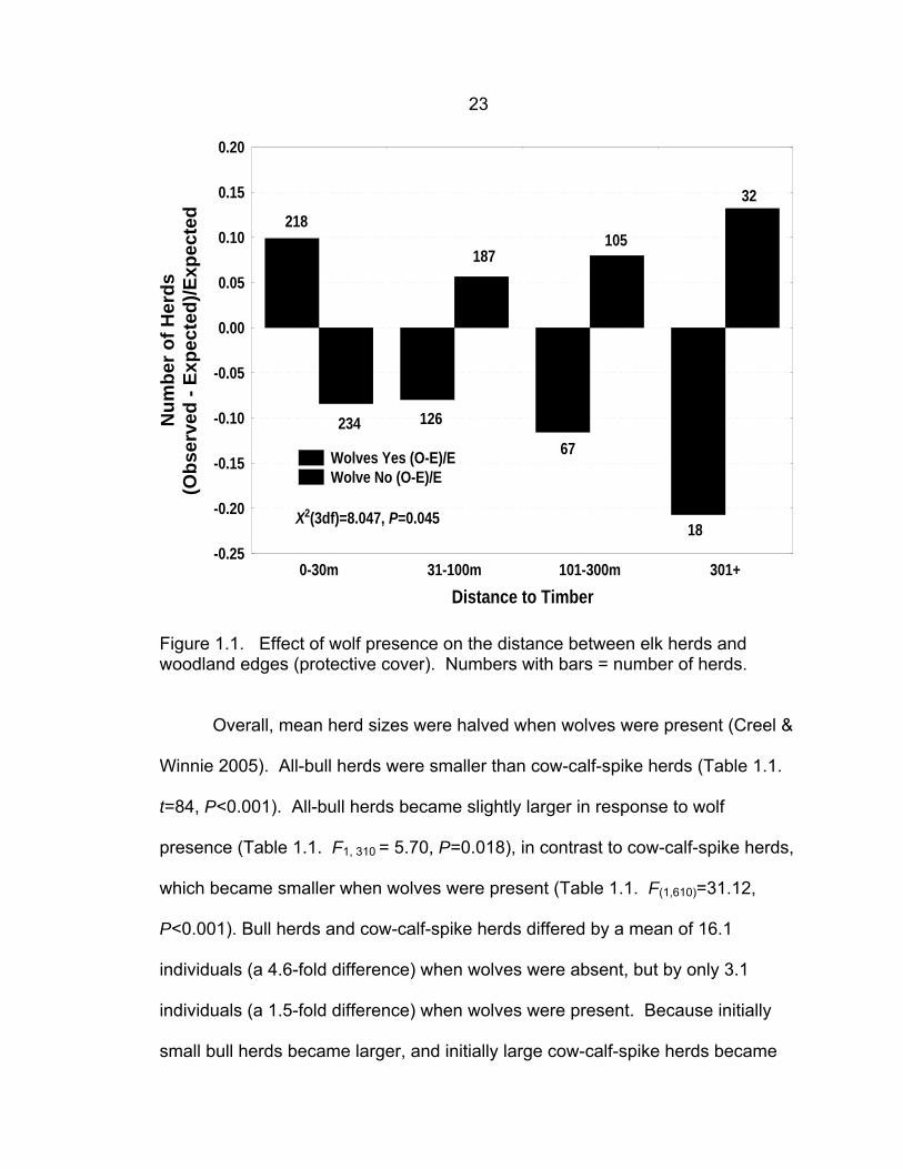
23
0-30m 31-100m 101-300m 301+Distance to Timber
-0.25
-0.20
-0.15
-0.10
-0.05
0.00
0.05
0.10
0.15
0.20N
umbe
r of H
erds
(Obs
erve
d - E
xpec
ted)
/Exp
ecte
d
Wolves Yes (O-E)/E Wolve No (O-E)/E
X2(3df)=8.047, P=0.045
218
126
67
18
234
187105
32
Figure 1.1. Effect of wolf presence on the distance between elk herds and woodland edges (protective cover). Numbers with bars = number of herds.
Overall, mean herd sizes were halved when wolves were present (Creel &
Winnie 2005). All-bull herds were smaller than cow-calf-spike herds (Table 1.1.
t=84, P<0.001). All-bull herds became slightly larger in response to wolf
presence (Table 1.1. F1, 310 = 5.70, P=0.018), in contrast to cow-calf-spike herds,
which became smaller when wolves were present (Table 1.1. F(1,610)=31.12,
P<0.001). Bull herds and cow-calf-spike herds differed by a mean of 16.1
individuals (a 4.6-fold difference) when wolves were absent, but by only 3.1
individuals (a 1.5-fold difference) when wolves were present. Because initially
small bull herds became larger, and initially large cow-calf-spike herds became

24
smaller, herds of all compositions converged to mean sizes of 6-9 elk when
wolves were present. In other words, variation in herd size decreased in
response to the presence of wolves.
Overall Wolves Absent Wolves Present Bull-only Herds 5.12, (4.48, 5.76) 4.472, (3.75, 5.19) 6.03, (4.88, 7.18)
Cow, Calf, Spike Herds 15.14, (13.08, 17.2) 20.58, (17.8, 23.4) 9.14, (6.22, 12.06)
Table 1.1. Herd size changes in relation to wolf presence (mean, 95% CI).
Marrow Fat and Individual Predation Risk Wolf-killed bulls were in poorer condition than wolf-killed cows throughout
the winter, as measured by marrow fat concentration (Fig 1.2: F1, 29 = 22.55, P <
0.001). Overall, the mean marrow fat content in bulls (0.35 proportion fat by
mass, 95% CI =0.27, 0.42) was half that of cows (0.70, 95% CI = 0.57, 0.83).
Marrow fat reserves in wolf-killed individuals of both sexes declined from early
winter to spring (F1, 29 = 23.704, P < 0.001, early mean = 0.70, 95% CI = 0.61,
0.90; late mean = 0.34, 95% CI = 0.22, 0.46). The interaction between the
effects of sex and season on marrow fat was weak (Fig. 1.2. F1, 29 = 1.86, P =
0.183).
Differences in body condition mirrored the patterns of predation reported
by Creel and Winnie (2005), where rates of predation differed from expected for
all age-sex classes (χ2= 39.21, df = 2, P < 0.001). Adult females were killed one-
third as often as expected by chance, while bulls and calves were killed 2.2-fold

25
and 2.5-fold more often than expected by chance, respectively. From the
perspective of an individual elk, the risk of being killed by wolves was 6.3 times
higher for a bull than for a cow. Because our marrow data are not a random
sample of the population at large, in isolation they do not allow a strong
conclusion that bulls are in worse condition than cows. However, when
considered alongside the work of others indicating that live bulls are in worse
condition than live cows in the winter (Anderson et al. 1972; Mitchell et al. 1976;
Geist 2002; Hudson et al. 2002), these data reasonably lead to the conclusion
that bulls in this population (as elsewhere) face stronger winter foraging
constraints than cows.
Early LatePeriod of Winter
0.0
0.2
0.4
0.6
0.8
1.0
1.2
1.4
1.6
Prop
ortio
n of
Fat
in M
arro
w (A
rcSi
n)
Cows
Bulls
Figure 1.2. Sex differences and winter changes in physical condition, as measured by femur marrow fat concentration.

26
Moving, Bedding and Other Behavior Moving, bedding and other behaviors accounted for 8.6%, 12.1%, and 2%,
of behavioral time budgets, respectively. The proportion of time spent moving
and bedding were unaffected by wolf presence, position in herd, or sex (Table
1.2). There was an overall decrease in other behaviors when wolves were
present, driven primarily by bulls (Table 1.2. F(1, 160)=6.8848, P=0.0095), and
while we did not formally break other down into sub-classes, our field notes
indicate this was probably due to bulls not sparring when wolves were present.
Because our study period was well past the fall rut, the sparring we observed
tended to be a relatively gentle but noisy rattling of antlers, limited to all-bull
herds.
The proportion of time spent moving did not change with distance to
timber (Table 1.2b). However, there was an interaction between wolf presence,
sex, and distance to timber (Table 1.2b. F(3,79)=3.19, P=0.028), driven by high
cow movements in the 0 to 30 m class when wolves were absent. A possible
explanation for this is that areas near timber are more heavily grazed than those
far from timber when wolves are present (Fig. 1.1) and that elk are simply more
likely to be moving through this zone to preferred foraging areas farther from
timber when wolves are absent. Because our data collection was not structured
to address this issue, it does not affect our general conclusions.

27
A Vigilance Grazing Moving Bedding Other Wolf Presence
F(1, 160)=1.145, P=0.286
F(1, 160)=0.301, P=0.584
F(1,160)=0.16, P=0.69
F(1,160)=0.09, P=0.76
F(1,160)=7.33, P=0.008
Sex F(1, 160) = 9.19, P=0.0028
F(1, 160)=1.63, P=0.2
F(1,160)=0.01, P=0.91
F(1,160)=0.65, P=0.42
F(1,160)=0.05, P=0.82
Position F(1, 160)=2.81, P=0.0956
F(1, 160)=2.85, P=0.093
F(1,160)=0.95, P=0.33
F(1,160)=0.24, P=0.63
F(1,160)=0.25, P=0.62
Wolf Presence x Sex
F(1, 160)=5.27, P=0.023
F(1, 160)=4.79, P=0.03
F(1,160)=2.14, P=0.15
F(1,160)=2.22, P=0.14
F(1,160)=6.88, P=0.01
Wolf Presence x Position
F(1, 160)=1.47, P=0.227
F(1, 160)=0.35, P=0.554
F(1, 160)=0.43. P=0.51
F(1, 160)=.07, P=0.79
F(1,160)<0.01, P=0.99
Sex x Position
F(1, 160)=0.08, P=0.78
F(1, 160)=0.48, P=0.49
F(1, 160)=0.1, P=0.76
F(1, 160)=0.22, P=0.64
F(1,160)=0, P=1.0
Wolf Pres. x Sex x Position
F(1, 160)=0.59, P=0.442
F(1,160)=0.09, P=0.77
F(1, 160)=0.09. P=0.76
F(1, 160)=0.5, P=0.48
F(1,160)=0.71, P=0.4
B Distance to Timber
F(3, 79)=0.09, P=0.965
F(3, 79)=0.627, P=0.6
F(3, 79)=0.406, P=0.749
F(3, 79)=1.148, P=0.34
F(1,160)=0.05, P=0.95
Wolf Presence x Dist. To Timber F(3, 79)=1.36, P=0.26
F(3,79) = 0.81, P=0.492
F(3,79) = 2.258, P=0.088
F(3,79) = 1.52, P=0.216
F(1,160)=1.55, P=0.22
Sex x Dist. to Timber F(3, 79)=0.07, P=0.98
F(3, 79)=0.55, P=0.65
F(3, 79)=0.528, P=0.664
F(3,79) = 0.425, P=0.736
F(1,160)=0.44, P=0.65
Wolf Pres. x Sex x Dist. to Timber
F(3, 79)=1.05, P=0.375
F(3, 79)= 0.56, P=0.65
F(3, 79)= 3.19, P=0.028
F(3,79) = 1.643, P=0.186
F(1,160)=0.26, P=0.77
Table 1.2. Associations between elk behavior and sex, location, position within herd, and wolf presence. Part b presents an analysis separate from the main factorial ANOVA, addressing the effects of distance to timber (see methods for details). Vigilance and Grazing Behavior Vigilance is the behavior most often traded with foraging (Lima & Dill 1990;
Lima 1998), and our results confirm this relationship. An increase in the
proportion of time spent vigilant can reasonably be considered a direct response

28
to elevated risk, and the corresponding decrease in foraging time as a cost of this
vigilance. Vigilance and grazing accounted for 15.8% (bedded vigilant: 4.9%;
standing vigilant: 10.9%) and 61.5% of all behaviors we recorded respectively.
Overall mean levels of vigilance and grazing did not change in response to wolf
presence (main effects: vigilance: F 1, 160 = 1.145, P = 0.286; grazing: F1, 160 =
0.301, P = 0.584) and the proportion of time spent grazing did not differ between
cows and bulls (F1, 160 = 1.63, P = 0.20). However, there was an interaction
between gender and wolf presence. Vigilance was higher in cows than in bulls
(F1, 160 = 9.19, P = 0.003). The difference in vigilance between the sexes was
driven by cows increasing their vigilance when wolves were present, while bulls
did not (Fig. 1.3. wolf x sex interaction: F1, 160 = 5.2733, P = 0.023). There was a
corresponding decrease in the proportion of time cows spent grazing when
wolves were present (Fig. 1.4. wolf x sex interaction: F1, 160 = 4.79, P = 0.03).
Overall, elk on the periphery of herds tended to be more vigilant and graze
less than interior animals, (vigilance: F1, 160 = 2.81, P=0.096; grazing: F1, 160 =
2.850, P = 0.093). Vigilance and grazing did not change with distance to timber
(vigilance: F3, 79 = 0.091, P = 0.965; grazing: F3, 79 = 0.627, P = 0.60). Similarly,
vigilance and grazing did not vary with herd size (vigilance: r2 = 0.007, F (1,86) =
0.64 , P = 0.43; grazing: r2 = 0.008, F (1,86) =0.70, P = 0.40).

29
Wolves Absent Wolves Present
0.2
0.3
0.4
0.5
Prop
ortio
n of
Tim
e Vi
gila
nt (A
rcSi
n) COWS
BULLS
Figure 1.3. Vigilance differences between the sexes in behavioral responses to the presence of wolves.
Wolves Absent Wolves Present0.6
0.7
0.8
0.9
1.0
1.1
1.2
Prop
ortio
n G
razi
ng (A
rcSi
n)
BULLS
COWS
Figure 1.4. Grazing differences between the sexes in behavioral responses to the presence of wolves.

30
Discussion
Our results show that elk do not categorize areas far from timber as
inherently dangerous, because mean vigilance levels do not increase with
distance to timber. This is surprising in light of our previous work indicating that
elk in our study area were disproportionately likely to be killed in open areas far
from timber (Creel & Winnie 2005). These areas are used primarily when the
temporal risk of predation is low (Fig. 1.1), and vigilance levels only increase (in
cows) when temporal risk is high (Fig. 1.3). The antipredator behavior of elk is
sensitive to both temporal and spatial variation in risk, so that areas that are only
dangerous in the presence of wolves do not provoke an increase in vigilance
(with its associated decrease in foraging) when wolves are absent. Moreover,
temporal variation in risk produces stronger antipredator responses in cows than
in bulls (Fig. 1.3), as expected based on cows’ greater latitude to pay the
associated foraging costs (Hudson et al. 2002; Geist 2002; Cook et al. 2004)
(Fig. 1.2). These patterns suggest that antipredator responses are quite sensitive
to variation in both costs and benefits.
Because herd size decreases when wolves are present (Creel & Winnie
2005), it is clear that elk do not aggregate for increased security when far from
timber. This response is somewhat surprising in light of the large number of
studies that document antipredator benefits to grouping, and suggests that elk
may disaggregate to reduce the likelihood of being detected by wolves. An

31
individual’s risk of predation can be broken into 4 components that comprise the
sequence of predation (Creel & Creel 2002):
1) Encounter rates — the probability of being encountered by a predator.
2) Attack preferences — the probability that the predator will hunt, upon
encountering prey.
3) Hunting success — the probability that the predator will make a kill, upon
hunting.
4) Dilution of risk — the probability that a given individual will be the victim,
upon a kill being made.
Predation risk is the product of these four conditional probabilities. Each of the
first three probabilities can be altered by changes in individual and group
vigilance, habitat types occupied by prey, or a combination of these. All four can
be altered by group size. We would expect prey to attempt to minimize the
product of these probabilities through behavior responses (if available),
depending on the associated costs and ability of individuals to pay. However,
behavioral responses that reduce one or more of the above probabilities may
result in an offsetting, or partially offsetting, increase in one or more of the
remaining probabilities, as when increases in group size benefit individuals
through dilution of risk, but also increase encounter, attack, and predator success
rates (Creel & Creel 2002; Hebblewhite & Pletscher 2002). Factors affecting
hunting success and dilution of risk are relatively well studied, but we know
surprisingly little about the ways that prey change their behavior to manipulate
encounter and attack rates (Creel & Creel 2002). Logically, we would expect

32
antipredator behavior to be directed to the first two stages in predator-prey
systems in which hunting success (stage 3) is difficult or energetically expensive
for prey to reduce.
When wolves were present in drainages, habitats far from timber were
substantially more dangerous for elk, and ground census data show that herd
sizes decreased at all but the nearest distance to timber category, where they
already tended to be small (Creel & Winnie 2005). GPS telemetry shows that
elk move into timbered areas when wolves are present (Creel et al. 2005). The
results presented here further indicate that elk are taking refuge in and near
timber, and thus probably perceive this cover as protective rather than
obstructive (Lazarus & Symonds 1992). Without behavioral observations of elk
and wolves in timber, we cannot say with certainty which of the first three
probabilities are affected by reducing herd size and dispersing into timber, but it
is likely that these responses reduce the risk of detection. Moreover, these
responses clearly come at the expense of dilution (at the level of single herds),
because herd sizes are smaller in the presence of wolves.
Hebblewhite and Pletscher (2002) found that wolves in Alberta
encountered larger groups of elk more than expected. Similar findings with wild
dogs and their prey in Africa (Creel & Creel 2002), spiders and parasitoid wasps
(Uetz and Hieber 1994), and cichlids and guppies (Krause and Godin 1995),
suggest that at least one reason for elk to reduce herd size is to reduce
encounters with wolves. However, the mechanics of encounter and attack
reduction remain unclear: elk may be reducing their detectability by scattering

33
into timber; or wolves may be aware of these scattered small groups and avoid
hunting them due to the increased effort (reduced profitability) involved in
approaching and testing multiple small groups before a vulnerable individual is
found; or elk may gain tactical advantages that influence wolves’ decisions
whether or not to attack; or some combination of these.
Regardless of the mechanisms involved, the above discussion begs the
question, “if reducing group size reduces individuals’ encounter probabilities, why
be in groups at all?” If aggregation is a response to predation risk, the answer is
probably dilution of risk. Dilution benefits accrue rapidly as group size increases
above one, with the biggest gains occurring with the first few added individuals.
However, wolf hunting behavior indicates that there is an increase in detectability
or attractiveness to wolves as elk group size increases (Hebblewhite & Pletscher
2002), and this probably forces elk to balance these opposing effects. Trade-offs
between encounters with predators and dilution provide a coherent explanation
for the herd size responses of bull versus cow-calf-spike herds (recall that, when
wolves were present, bull herds increased slightly from 4.5 to 6, whereas cow-
calf-spike herds decreased from 20.5 to 9.1). These two types of herds make
different behavioral responses to the threat of predation to arrive at a common
solution – intermediate herd sizes of 6-9 elk. These results suggest that groups
of roughly 6-9 individuals may provide a balance between detectability (or
attractiveness to wolves) and dilution.
34
A large body of theoretical and empirical work has established that
foraging decisions and risk taking should both depend on body condition
(Houston & McNamara 1982; McNamara & Houston 1992; Bachman 1993;
Sinclair & Arcese 1995). In the Gallatin, wolves killed bulls more often than
expected by chance (Creel & Winnie 2005), and overselection of males in winter
is common in other studies of predation on large ungulates (Huggard 1993; Mech
et al. 2001). The poor condition of bulls during winter that we observed offers
insight into sex-differences in behavioral responses, and incidentally, the
mechanisms that might be driving sexual segregation. Wolf-killed bulls were in
worse physical condition than wolf-killed cows throughout the winter. Bulls were
significantly less vigilant than cows; did not respond to wolf presence with
increased vigilance; and formed groups less than half the overall mean herd size.
Our previous work has shown that individual bulls are roughly 6 times more likely
than cows to be killed by wolves (Creel & Winnie 2005), yet despite this relatively
high level of personal risk, bulls do not increase vigilance in response to wolf
presence. Bachman (1993) reported similar results where experimentally
starved ground-squirrels reduced vigilance levels in exchange for increased
foraging time, and were less responsive to the warning calls of conspecifics. If
the differences between wolf-killed bulls and live bulls are similar to differences
between wolf-killed cows and live cows, as previous research indicates they
probably are (Anderson et al. 1972; Mitchell et al. 1976; Geist 2002; Hudson et
al. 2002), then the above behavioral patterns suggest that bulls are less able to
pay the foraging costs of responding to wolf presence by increasing vigilance.

35
Despite the slight increase in herd size in response to elevated risk, bull
groups tended to be small, regardless of wolf presence (Table 1.1). This may be
driven by their lower ability to pay the costs of increased numbers of encounters.
Other studies suggest that large groups are encountered and attacked by
predators more often than expected by chance (Creel & Creel 2002; Hebblewhite
& Pletscher 2002; Krause and Godin 1995). Consequently, bulls may need to
avoid large groups (despite the benefits of risk-dilution) for two reasons. First,
encounters with wolves carry energetic costs that bulls are ill prepared to pay
due to poor condition. Second, the benefits of risk dilution are probably not
distributed evenly within herds. There is probably a set of relatively vulnerable
individuals within most herds from which the victim is selected, and rut-weakened
bulls, if present in these herds, are likely to be in this subset (Geist 2002). The
combination of the cost of more frequent encounters, and their relative
vulnerability given an encounter (hence reduced dilution benefits), may be
sufficient to keep bulls out of larger cow-calf-spike herds, thus promoting sexual
segregation.
There may be differences in the way that wolves select bulls and cows
based on condition. Bulls, about 30% larger than cows and carrying antlers, may
represent a more dangerous adversary than cows, so that wolves do not risk
attacking them until they are in worse condition. Given our data, we can not
directly assess this aspect of prey selection, but the fact that wolf-killed bulls
have significantly lower marrow fat than wolf-killed cows suggests that wolves
may select males only when they fall below a threshold of vulnerability.

36
Furthermore, this threshold of vulnerability may be relative – depending on the
current condition of otherwise more vulnerable cows.
In contrast to bulls, cows employ a broad set of responses to elevated
threat that operate at multiple scales: cows increase individual vigilance levels at
the expense of grazing, reduce group size, and move closer to or into timber.
Despite the behavioral responses of cows, calves suffer higher rates of predation
than expected by chance (Creel & Winnie 2005). Calves are dependent upon
their mothers and do not have the option of leaving large mixed herds, as bulls
do, when wolves are present (Creel & Winnie 2005). When these herds are
attacked (despite the behavioral responses of the cows), calves may be singled
out by attacking wolves. The high vulnerability of calves to predation may in part
contribute to the strong behavioral responses of cows seeking to protect not just
themselves, but also a substantial reproductive investment in their current calf.
We cannot assess the absolute effectiveness of cow behavioral
responses, but in parallel with their behavioral responsiveness, they experience a
low rate of predation in comparison to bulls. If the antipredator behavior of cows
is relatively effective when compared to bulls, this may be all that is necessary.
Savino and Stein (1989) examined the effects of prey behavioral responses and
habitat selection on predation rates in fish. In an environment containing 2
species each of predators and prey, the prey species that shifted from open to
closed habitats markedly decreased its risk of predation, while the prey species
that did not respond suffered increased predation. Elk of different sexes display
a similar dichotomy of behavior, with a similar pattern of predation. The lack of

37
effective behavioral responses by bulls may increase the effectiveness of cow
responses – cows make themselves unavailable to wolves relative to bulls. Bulls
then bear the brunt of wolf predation because of their inability to pay the costs
associated with more effective anti-predator behavior.
Grazing and vigilance levels were unaffected by herd size or distance to
timber (main effects, Table 1.2). It appears that, regardless of local elk density or
habitat quality, Gallatin elk consistently attempt to maximize forage intake in
winter, and only when faced with imminent danger (the presence of wolves in the
drainage), are they willing to reduce feeding time in exchange for increased
vigilance (cows), or compromise forage quality by moving nearer and into timber
(both sexes).
Elk in the upper Gallatin assess spatial variation in predation risk at fine
scales, on the order of meters, and temporal variation in risk on the order of a
single day (or less). Moreover, spatial and temporal variation in risk interact and
this is reflected in the behavioral responses of elk. These variations in risk drive
a suite of anti-predator behavioral responses that depend on gender and physical
condition, apparently constrained by individuals’ ability to pay the associated cost
in foraging time. Despite heavy over-selection by wolves in our study system,
bulls did not increase vigilance when wolves were present in a drainage. This
implies that the foraging costs of increased vigilance are substantial, yet these
foraging costs are being paid by cows at a time when most are carrying
developing fetuses (Cook 2002; Hudson et al. 2002; Cook et al. 2004). These

38
antipredator responses create indirect costs of predation which may affect prey
demography through survival or reproduction.
All of these responses occur on a time scale that corresponds to the
comings and goings of wolves, and a spatial scale defined by the movements of
elk on that time scale, which is substantially smaller than a complete wolf
territory. These results are relevant to current debate over wolf-elk-plant trophic
cascades in the Yellowstone ecosystem: to date, direct data on the responses of
elk to wolves have been lacking, making it difficult to disentangle elk effects from
myriad other influences on surrounding plant communities. This emphasizes the
necessity of observing prey behavioral responses to risk on the scales at which
important variation in risk actually occurs.
39
CHAPTER 3
ELK DECISION-MAKING RULES ARE SIMPLIFIED
IN THE PRESENCE OF WOLVES
Abstract
The risk of predation drives many behavioral responses in prey. However,
few studies have directly tested whether predation risk alters the way other
variables influence prey behavior. Here we use information theory (AICc) in a
novel way to test the hypothesis that the decision-making rules governing elk
behavior are simplified by the presence of wolves. With elk habitat use as the
dependent variable, we test whether the number of independent variables (i.e.
the size of the models) that best predict this behavior differ when wolves are
present versus absent. Thus, we use AICc scores simply to determine the
number of variables to which elk respond when making decisions. We
measured habitat use using 2288 locations from GPS collars on 14 elk, over two
winters (14 elk winters), in the Gallatin Canyon portion of the Greater
Yellowstone Ecosystem. We found that use of three major habitat components
(grass, conifer, sage) was sensitive to many variables on days that wolves were
locally absent, with the best models (∆AICc ≤ 2) averaging 7.4 parameters. In
contrast, habitat use was sensitive to few variables on days when wolves were
present: the best models averaged only 2.5 parameters. Because fewer
variables affect elk behavior in the presence of wolves, we conclude that elk use

40
simpler decision-making rules in the presence of wolves. This simplification of
decision-making rules implies subtle, but potentially important, constraints that
predation risk imposes on prey behavior, by reducing prey’s ability to optimize
foraging and movement.
Introduction
When faced with the threat of predation, most animals engage in
behaviors that reduce risk, and selection should favor individuals who best
balance the benefits of risk reduction against its costs (Lima & Dill 1990; Illius &
Fitzgibbon 1994). Responses to predation risk include increased vigilance (Elgar
1989; Lima and Dill 1990), reduced foraging time (Hughes & Ward 1993;
Abramsky et al. 2002), reduced movement (Sih & McCarthy 2002), reduced use
of conspicuous behavioral displays (Sih et al. 1990), changes in group size (Lima
& Dill 1990; Creel & Winnie 2005), and habitat shifts (e.g. retreat to low risk areas
or refuges: Bergerud et al. 1983; Formanowicz & Bobka 1988; Blumstein &
Daniel 2002; Heithaus and Dill 2002).
The above studies address direct behavioral responses to the threat of
predation. However, prey must do more than simply manage predation risk to
survive (Lima and Dill 1990), and shifting habitats in response to predators will
interact with other important demands. Regardless of the presence of predators,
most prey species must move about the environment frequently and forage to
meet their daily needs, and variables unrelated to risk should also affect foraging
behavior and movements.

41
There is an emerging literature on decision-making that addresses the
use of simple heuristics or rules-of-thumb, versus complex optimization
algorithms (Hutchinson and Gigerenzer 2005; Kemp 2005). This literature
suggests that simple rules produce more general solutions, but complex
optimization strategies produce better solutions to specific problems. In this
paper, we use data on habitat use by elk to test whether predation risk affects the
complexity of decision-making rules.
When prey are unconstrained by risk, their foraging decisions might be
optimized by using a wide range of information and responding to many
variables. Conversely, predator-induced constraints may force prey to forego
complex decision making strategies, and resort to simpler algorithms, or rules-of-
thumb (Kemp 2005). Prey decision-making rules may further be constrained if
preferred foraging environments are not the same as escape terrain. When
predators are absent, foraging prey may accumulate relatively little information
about escape terrain. If this is the case, prey engaging in a spatial shift to
escape terrain in response to elevated risk may not have the information
necessary to optimize their behavior in a habitat-specific manner, and be forced
to resort to simpler algorithms, or rules of thumb when making foraging and
movement decisions.
In the winter, elk in the Upper Gallatin River drainage respond to short-
term changes in the threat of wolf predation at multiple scales: individual, herd
and landscape. When wolves are present in a drainage, some individuals
(females) increase vigilance at the expense of foraging (Winnie and Creel, in
42
review), mean herd size decreases and herd composition changes (Creel and
Winnie, 2005), and elk leave open grassy areas and move into the protective
cover of timbered areas (Creel et al 2005). These responses appear to be
constrained by body condition, indicating that antipredator behaviors carry
foraging costs (Winnie and Creel in review).
Regardless of the presence of wolves, elk move about the landscape to
forage, and we would expect that foraging and movement are affected by
variables other than risk. Net energy and protein content differ between woody
browse and grasses (Christianson and Creel in press), and both the availability of
plants and foraging costs are affected by interactions between growth form and
snow conditions (Jenkins and Wright 1987). Thus, we might expect elk behavior
to be affected by differences in snow depth and snow density across local
landscapes (Sweeney and Sweeney 1984). Elk of both sexes face a negative
energy budget in winter, but males appear to face stronger energetic constraints
because they enter winter with depleted energy stores following the fall rut (Geist
2002; Winnie & Creel in review). Consequently, we might expect gender to play
a role in behavior. Winter weather in the Northern Rockies can be extreme even
for cold-adapted species, so we might expect rules for selection of open and
closed habitats to be sensitive to temperature and wind speed (Merrill 1991;
Jones et al 2002).
Differences in elk decision making rules should be reflected in differences
in models that best describe their behavior. Here, we test the hypothesis that the
rules by which elk select habitats are simplified by the presence of wolves

43
Specifically, when elk are unconstrained by predation risk, models describing
behavior should contain more parameters, and conversely, when risk is high,
models should contain fewer parameters.
Methods
Study Area
Our study area is a mosaic of National Forest, National Park, State, and
private land, covering 125.8 km2 in four drainages along the upper Gallatin River
(Porcupine [30.3 km2], Taylor [56.0 km2], Tepee [13.1 km2] and Daly [26.4 km2]).
South-facing slopes and valley bottoms are generally a mixture of open sage
(Artemesia spp.) and grassland (dominated by Idaho fescue and bluebunch
wheatgrass: Festuca idahoensis & Agropyron spicatum) with riparian areas
bordering creeks. North-facing slopes and higher elevations are primarily
coniferous forest (lodgepole pine and Douglas fir: Pinus contorta & Pseudotsuga
menziessii) broken by occasional small meadows. Elevation runs from 1975 m
ASL to 2432 m ASL.
We surveyed fixed areas (viewsheds) in each of the four drainages,
beginning at first light, every two-weeks from mid- January, 2002 until the end of
May, 2002, and during the same period in 2003, and recorded all wolves, elk and
elk carcasses located in these surveys. Survey routes were chosen to maximize
the area scanned in each drainage while minimizing disturbance caused by our
presence. During a survey, we scanned from fixed highpoints and while walking
fixed routes between highpoints. Each drainage was divided into 6-8 viewsheds.

44
In addition to this formal sampling regimen, we attempted to visit each drainage
on every day of the winter-spring study period, in either the morning or evening,
usually traversing part of our fixed sampling routes. These ad-lib samples
provided additional information on wolf presence (see Wolf Presence below).
Elk The elk in the study area are part of a largely migratory population
(averaging 1725 [se 63] and varying from 1214 to 3028 animals annually since
1928) that winters along the upper Gallatin River and its tributaries from the
northwest corner of Yellowstone National Park, north to Big Sky, Montana
(Brazda 1953; Peek et al 1967; Peek and Lovaas 1968). Both the migration
route and winter range encompass state, private, and federal lands, while the
summer range for most of the elk lies within western Yellowstone National Park.
We designed and built data-logging GPS units based on SiRFstar I GPS
engines (SiRF Technology, San Jose, California) and riveted them to the tops of
conventional VHF radio collars equipped with timed drop-off mechanisms
(Advanced Telemetry Systems, Inc., Isanti, Minnesota, USA). We collared 7 elk
each winter (10 adult females, 4 adult males) for a total of 14 elk winters. Each
collar was set to fix every 2 hours, and the mean realized fix rate was 61.7%
(mean fix interval of 3.24 hours), yielding 18,317 fixes. Of these fixes, 2288 fell
in winter periods in study drainages at times for which we data on wolf presence
or absence. We tested for differences in fix rate between forested and open
habitat types and found no significant differences (forested F=1.67, P=0.196;

45
open F=0.88; P=0.35). Wolf presence or absence in a drainage did not
detectably alter the fix rate (F = 0.88, P = 0.35).
Wolves Wolves colonized the upper Gallatin drainage in 1997, and during the
course of this study, 2 packs (12-16 wolves) used the study area each year.
We used a combination of direct observations, conventional VHF collars, snow
tracking, and detection of scats and wolf kills to determine wolf presence in each
of the study drainages on each day. While walking survey routes or collecting
ad-lib behavioral observations, we continuously checked for signs of wolves. We
considered wolves present within a drainage on a given day if we located them
via VHF radiotelemetry, found a fresh kill, fresh scat, or fresh tracks in snow, mud
or loose soil. We considered wolves absent from a drainage if we surveyed and
detected no sign of wolf presence for that day. For days that a drainage was not
surveyed, we excluded the GPS data. If wolves denned in a drainage (near April
15th both years), we scored wolves as present in that drainage on all days during
the denning period. Because not all wolves in the study area were radiocollared
and we undoubtedly missed some physical evidence of their presence, it is likely
that we failed to detect wolves on some days. This failure to detect wolf
presence might mask responses by elk to wolves (Type II errors), but should not
create apparent differences where none exist (Type I errors), so tests comparing
data from wolf present and wolf absent conditions are conservative.

46
Our work in this study system (Creel & Winnie 2005; Creel et al. 2005;
Winnie & Creel in review) has shown that elk respond to the presence and
absence of wolves at the scale of our data and analyses, both temporally (days
and hours) and spatially (drainages, broad habitat types measured at 30m
pixels). Of course, this does not mean that elk do not also respond to wolves at
other spatial and temporal scales (see Discussion).
Habitat Composition at Elk Locations
To assess habitat types at elk GPS locations, we applied logistic
regression models for the probability of occurrence of dominant plant species,
developed for Yellowstone’s Northern Range (Rew et. al., 2005; Rew et al, in
press). These regressions were selected using AICc via single term deletions
from a full model including slope, elevation, sine (E/W) and cosine (N/S) of
aspect, and seven bands of Landsat 7 ETM reflectance data. Model selection via
single term additions yielded the same result in all cases. We validated the
regression models using 315 sampling locations stratified by drainage and
elevation across the Gallatin study site. To simplify the analysis of habitat
selection by elk, we combined probabilities of occurrence for all conifer species
(lodgepole pine, limber pine, subalpine fir, Douglas fir, and Englemann spruce)
into one habitat component (conifers), combined the probabilities of occurrence
for the two dominant native grasses (bluebunch wheatgrass and Idaho fescue)
into a second component (grass), and combined sage species (big sage,
Artemesia tridentata and silver sage A. cana) into a third component (sage).
47
Using ArcGIS, each elk location was assigned separate probabilities of conifer
occurrence, grass occurrence, and sage occurrence. The use of three
probabilities is probably an oversimplification of how elk perceive habitats, but
our previous work (Creel et al 2005; Winnie and Creel in review) has shown that
these probabilities (dependent variables) do respond to wolf presence in this
system. To test the hypothesis that the complexity of decision-making rules
responds to predation risk, all that is required are dependent variables known to
be affected by risk.
Each habitat component is modeled independently of the other two
components, so the three probabilities of occurrence need not sum to 1. This is
appropriate, because many locations have a high likelihood of more than one
habitat component being present. This approach incorporates continuous spatial
variation in preferred food (grass), protective cover (conifers), and sage, which is
associated with food but also may provide limited cover. Incidental properties of
this approach are that the probability of occurrence for each habitat component
on any pixel (30m x 30 m) was never 1 or 0 (the model was never absolutely
certain that a habitat component did or did not occur in a given pixel), and
probabilities did not share the same scale from model to model, i.e. relative
probabilities of occurrence are consistent across locations within a habitat model,
but probabilities of occurrence cannot be directly compared across habitat
models. This method of mapping habitat components is more descriptive than
simply categorizing habitats into three exclusive types, because it is unlikely that
elk perceive locations categorically, as one habitat type or another. Locations
48
are mixtures of food and cover that vary along continuous scales, and multiple
plant components can and do occur in the same patch (in the case of our
models, 30 x 30m pixels).
Environmental Variables We recorded temperature and wind speed during every trip to a drainage
using Kestrel pocket weather stations. During each bi-weekly survey trip up a
drainage, we gathered data on snow depth and density at three fixed monitoring
locations (at low, middle, and high elevations in each drainage). Sites at each
elevation consisted of a pair of open and timbered measurement areas within
50m of each other. We measured snow depth by digging down to dirt and using
a retractable tape measure. We measured snow density by dropping a 3 kg steel
shot attached to a cord from 30cm above the snow surface and recording the
depth of penetration. We express snow density as depth of penetration from a
30 cm drop divided by total depth, yielding numbers ranging from 0 to 1, with
numbers near 1 representing the least dense snow. At times and in places
where snow depth was 0, we scored snow density as 1, to reflect the fact that
snow did not impair access under this condition. We averaged depths and
densities for the three elevations within each drainage to get one mean snow
depth in the timber and one in the open and one snow density in the timber and
one in the open. We made snow depth and density measurements at two week
intervals in each drainage, and used linear interpolation between measurement
days to estimate daily values in each drainage. Because we collected these data

49
across the study site using a design stratified by drainage, elevation and habitat
type, we preferred them to daily data on snow-water-equivalent accumulation
from regional NRCS SNOTEL sites.
Statistical Analysis
To test our hypothesis, we compared the complexity of models that best fit
data on elk behavior in high and low risk conditions. We did this via model
selection using Akaike’s Information Criterion (AICc), applied in a novel way.
Typically, AICc is used to distinguish among competing hypotheses, each framed
as a regression model. Here, we used AICc simply to test whether well-
supported models included a larger set of independent variables when wolves
were absent. That is, we used AICc scores to identify models with good support
from the data, so that the number of parameters in these models could be used
in the next step.
Using the models identified by AICc, our intention shifted from identifying
strong models to testing hypotheses about the differences between model sets.
We performed three one-tailed t – tests, one for each habitat component. Each t-
test compared the mean number of parameters in the best models (within 2 AIC
units of the best model) when wolves present versus wolves absent (H0: the
number of parameters equal or greater when wolves present; Ha: fewer
parameters when wolves are present). Degrees of freedom were based on the
number of models within 2 AIC units of the best model, calculated conservatively
using a method that penalizes for high sample variance (Devore and Peck 2001).

50
Overall, the logic of our analysis is as follows. We hypothesized that the
presence of wolves (high predation risk) imposes constraints on habitat selection
rules. The models of habitat use selected when wolves are present identify the
number of variables to which elk respond when constrained by immediate risk.
Similarly, the models of habitat use selected when wolves are absent identify the
number of variables to which elk respond without the constraints of immediate
predation risk. We hypothesized that models would be larger (more complex)
when elk were unconstrained by predation risk and smaller when wolves were
present. We used ‘best subsets’ modeling, allowing elk to tell us how many
environmental variables were important to them when making habitat use
decisions. Because this approach yields a large model list, we limit all
subsequent inferences (including model averaging and calculating relative
variable importance) to models within 2 AIC units of the best model. Best
subsets modeling has been criticized as data dredging, in the normal context of
using AIC to compare a set of models, each of which represents a hypothesis of
direct interest (Burnham & Anderson 2002, Stephens et al. 2005). But we use
AIC only to determine the complexity of the best models under two conditions.
The hypothesis we test is that the model sets differ in the size of the models that
receive support from the data – a test to which the data-dredging criticism does
not apply.
To test how predation risk affected habitat selection rules, we divided the
elk GPS locations into two data sets based on differences in short-term predation
risk: wolves present versus wolves absent from that drainage on that day. For

51
each of the data sets (wolves present, wolves absent) we used model selection
based on information theory (using Akaike’s Information Criterion with sample
size correction, AICc) to identify the models that best predicted the probabilities
of occurrence of grass, sage, and conifer at elk locations. Thus, we compared
models of habitat selection for three dependent variables (habitat components),
each under two conditions (wolves present = high risk, wolves absent = low risk),
for a total of six model-selection analyses. We applied a log-odds transformation
to the dependent data log(y/((1-y)) that yielded an approximately normal
distribution, and specified an identity link to the independent variables.
Independent Variables. For each of the six dependent variables, our
independent variables were:
- Previous location. The attributes of an elk’s current location are related to
the attributes of its location two hours earlier, so treating all of the GPS
fixes as independent data points would cause pseudoreplication. To
avoid this, we used autoregression, including the value of the dependent
variable for the previous location in the time series as a predictor. We
tested whether the inclusion of more than one time lag improved the
model, but AICc scores strongly supported the single-lag model (Creel et
al. 2005). This procedure accounts for repeated measures and temporal
autocorrelation in the data while retaining all of the GPS fixes for
maximum valid power.

52
- Sex. Our previous work revealed behavioral differences between bulls
(branch antlered males) and cows (females > 1 year old) in their
responses to wolves (Winnie and Creel in review).
- Minimum recorded temperature in each drainage for that day.
- Maximum wind speed in each drainage on that day.
- Temperature x Wind Speed interaction (minimum x maximum,
respectively).
- Depth of snow in the open.
- Depth of snow in timber.
- Density of snow in the open.
- Density of snow in timber.
- Day of year, beginning January 1st. This variable incorporates three
effects that we did not measure directly. Forage quality declines as winter
progresses (Demarchi, 1968). Forage quantity also declines because this
was a winter study, and there was no plant re-growth after grazing and
browsing. Finally, body condition declines, due to the interaction of the
declining forage quantity and quality with high winter metabolic demands.
Declining body condition through winter has been reported in other
ungulate studies, and we have presented evidence for elk in this system
(Winnie and Creel in review). This factor is problematic because it is
correlated with temperature and snow depth, and thus contributes to
overdispersion in models that also contain these variables.
53
Because regression models (and parameter estimates) can be expected
to differ from one data set to another, it is important to keep in mind that these
analyses use six discrete data sets (predicting 3 habitat variables under two
levels of risk). Thus, differences in parameter estimates between models should
be interpreted cautiously and we limit our inferences to overall differences
between sets of model-averaged parameters.
Results and Discussion
The attributes of elk GPS locations and global model goodness-of-fit,
when wolves were present and absent are summarized in Table 2.1. Model
selection revealed marked and consistent differences in the number of
parameters that influenced elk behavior when wolves were present versus
absent. The probability of occurrence of all three habitat components at elk GPS
locations was best predicted by models with many environmental parameters
when wolves were absent, and fewer parameters when wolves were present:
conifers wolves present mean 2.2, wolves absent mean 7.2, (t0.05(1), 22 = 12.6, p <
0.0001); sage wolves present mean 2.2, wolves absent mean 6.7 (t0.05(1),33 =
11.9, p < 0.0001); grass wolves present mean 2.0, wolves absent mean 8.2
(t0.05(1),7 = 21.4, p < 0.0001).

54
Wolves Absent Global Model Log Odds N Mean Min. Max. SD CV R2 F (10 DF) P Conifer 1604 -2.31 -4.42 0.15 1.03 44.35 0.09 14.9 <0.0001 Grass 1604 -0.32 -2.22 1.53 0.74 229.73 0.06 10.01 <0.0001 Sage 1604 -0.40 -3.24 2.14 1.14 282.98 0.04 6.5 <0.0001
Wolves Present Log Odds N Mean Min. Max. SD CV R2 F (10 DF) P Conifer 684 -1.69 -4.50 0.52 1.19 70.09 0.06 4.22 <0.0001 Grass 684 -0.82 -2.32 2.50 0.78 95.30 0.04 2.75 0.0030 Sage 684 -1.15 -3.46 1.93 1.24 107.16 0.06 3.68 <.0001
Table 2.1. Habitat attributes of elk GPS locations with wolves present and absent, and global model goodness-of-fit. 1Lower log-odds indicate a lower probability of occurrence of a habitat component. * Autocorrelation in these data are accounted for in the analysis, see methods.
When wolves were absent, several models within two AIC units of the best
model included 8 or more parameters (overall wolves absent: mean = 7.42
parameters in the top models: Figures 2.1a, b, c). For conifers, the global model
(10 parameters) was in the set of best models. In particular, parameters
describing snow conditions significantly affected the occurrence of all three
habitat components at elk locations, and appeared in most of the top models
when wolves were absent (Appendix A).
When wolves were present, the best models describing elk behavior were
much simpler. Most of the top models contained 2 parameters, and none had
more than 4 (wolves present: mean = 2.46 parameters). For all three habitat
components, previous location alone was the best model, based on AICc scores
(Figure 2.1a, b, c and Appendix A). Given this, the worst ∆AICc score that any
two parameter model could attain when wolves were present was two AIC units
worse than previous location alone. Consequently, for all of the two parameter

55
models with ∆AICc values near 2, the second parameter has relatively little effect
on habitat use (Tables 2.2 & 2.3, Appendix A). This is reflected in the parameter
estimates and their standard errors (Table 2.2), and in relative importance values
(Burnham & Anderson 2002) for each variable (Table 2.3). No factors other than
previous location had significant effects on habitat use at α = 0.05 (Table 2.2),
and no factors other than previous location had relative importance approaching
1 when wolves were present (Table 2.3).
Differences in the complexity of the models suggest differences in the
rules that elk use to make decisions about habitat use. In the absence of wolves,
elk respond to many environmental factors, particularly snow conditions, when
making habitat use decisions. On days that wolves were absent, the probability
of both conifer and grass occurrence at elk locations is sensitive to snow depth
and density in both open and forested areas (Tables 2.2 & 2.3). Sensitivity to
environmental conditions is probably a response to the combination of poor
winter food quality and the energetic costs of moving and foraging in snow.
Frequent adjustments to movements and foraging locations based on fine
temporal and spatial scale information about snow conditions may be necessary
to optimize trade-offs between energy expenditure and intake. For elk in winter,
facing a long-term negative energy budget (Cook 2002, Hudson et al 2002),
selection pressures on this optimization are likely to be strong.

Conifer Models (all models within 2 AIC units of the best model)
0 1 2 3 4 5 6 7 8 9 10 11Number of Model Parameters
1
2
3
4
5
6
7
8
9
10
Mod
el R
ank
Wolves Absent Wolves Present
Global Model
Figure 2.1a.
Grass Models(all models within 2 AIC units of the best model)
0 1 2 3 4 5 6 7 8 9 10 11Number of Model Parameters
123456789
10111213
Mod
el R
ank
Wolves Absent Wolves Present
Global Model
Figure 2.1b.
Sage Models(all models within 2 AIC units of the best model)
0 1 2 3 4 5 6 7 8 9 10 11Number of Model Parameters
123456789
1011121314151617181920212223
Mod
el R
ank Wolves Absent
Wolves Present
Global Model 56 Figure 2.1c. Figure 2.1a, b, c. Summary of the best models of habitat selection by elk, identified via Akaike’s Information Criterion. Each panel summarizes the set of best models for a given habitat component, for data with wolves absent (black bars) and present (crosshatched bars). (a) conifers, (b) grassland, (c) sage. See Appendix A for details of each model.

57
Parameter Estimates from Model Averaging (bold indicates 95% CI does not contain 0) Conifer Grass Sage
Wolves Absent Wolves Present Wolves Absent Wolves Present Wolves Absent Wolves Present
-0.960 -1.370 -0.520 -0.620 -1.230 -1.500 Parameter Estimate SE Estimate SE Estimate SE Estimate SE Estimate SE Estimate SE
Previous Location 0.214 0.025 0.250 0.038 0.183 0.025 0.118 0.133 0.147 0.025 0.201 0.039Sex -0.115 0.042 0.000 0.056 0.060 0.031 0.014 0.038 0.046 0.046 -0.035 0.059
Day of Year 0.004 0.003 0.001 0.002 -0.004 0.002 0.000 0.001 -0.006 0.003 0.004 0.006
Temperature -0.008 0.006 0.001 0.008 0.003 0.004 -0.004 0.006 0.008 0.006 -0.005 0.010
Wind Speed -0.012 0.007 0.003 0.012 0.006 0.005 0.007 0.008 0.015 0.008 0.000 0.013
Temp. x Wind -0.003 0.001 0.001 0.002 0.001 0.001 -0.002 0.001 0.002 0.001 -0.001 0.002
Snow Depth Open 0.012 0.004 -0.001 0.002 -0.010 0.003 0.059 0.075 -0.010 0.004 0.025 0.017
Snow Depth Timber -0.012 0.004 0.000 0.003 0.007 0.003 -0.003 0.339 0.006 0.005 -0.037 0.024
Snow Density Open 0.272 0.111 -0.206 0.226 -0.214 0.081 0.097 0.153 -0.199 0.123 0.574 0.383
Snow Density Timber -0.405 0.158 -0.149 0.337 0.277 0.116 0.165 0.226 0.303 0.177 -0.844 0.757
Table 2.2. Coefficients and their standard errors from model averaging using AICc weights (ωi). Coefficients reported separately for each habitat component under each predation-risk condition. Bold entries indicate parameters that differ from zero at α = 0.05). Deviance/DF (ĉ) for each global model is reported in parentheses under wolf presence headings. Relative Importance
Conifer Grass Sage Wolves Wolves Wolves Wolves Wolves Wolves
Parameter Absent Present Absent Present Absent Present Previous Location 1.000 1.000 1.000 1.000 1.000 1.000 Sex 1.000 0.081 0.901 0.062 0.232 0.043 Day of Year 0.677 0.081 1.000 0.059 0.900 0.151 Temperature 0.427 0.081 0.216 0.132 0.367 0.118 Wind Speed 0.581 0.083 0.287 0.082 0.931 0.038 Temp. x Wind 0.923 0.094 0.600 0.117 0.774 0.082 Snow Depth Open 1.000 0.083 1.000 0.194 1.000 0.360 Snow Depth Timber 1.000 0.081 1.000 0.191 0.278 0.368 Snow Density Open 1.000 0.113 1.000 0.195 0.557 0.424 Snow Density Timber 1.000 0.086 1.000 0.067 0.804 0.344
Table 2.3. Relative importance values from AICc.

58
On days that wolves were present, the same elk, in the same drainages,
showed substantially less complexity in their decisions about habitat use. The
lack of sensitivity to snow conditions when wolves are present implies that elk are
not attempting to gain tactical antipredator advantages (or reduce tactical
disadvantages) by avoiding or favoring areas with particular snow conditions.
When combined with our previous research showing that elk retreat to the cover
of timbered areas when wolves are present (Creel and Winnie 2005; Winnie and
Creel in review), this result suggests (but does not prove) that elk spatial
responses are weighted towards avoiding encounters with wolves, rather than
manipulating the outcome of encounters. Alternatively, it is possible that the
temporal (bi-weekly) and spatial (open versus timbered) scales at which we
measured snow conditions were only able to detect conditions that mattered to
elk when they are unconstrained by predation risk. When wolves are present, elk
may be sensitive to snow conditions (and possibly other unmeasured variables)
at finer scales than we measured - i.e. fine enough scales to avoid terrain traps
created by deep and crusty snow if they are pursued by wolves.
The results of model selection for sage are not as clear as the results for
conifers and grass (Figure 2.1c.). This is not due to sage being uniformly
distributed among elk locations, because sage probability of occurrence has a
higher CV than either grass or conifer (Table 2.1). At the risk of telling Just So
Stories (Kipling1902), we believe this is because sage offers neither preferred
foraging habitat when wolves are absent, nor preferred cover when wolves are
present. When unconstrained by snow or predation risk, elk strongly prefer
59
grazing to browsing (Christianson and Creel in press), and when faced with
elevated predation risk they move to timber (Creel et al 2005, Winnie and Creel
in review). Anecdotally, from substantial experience walking on this study site,
moving through sage is particularly difficult. The complex plant structure collects
snow and creates suspended surfaces that collapse when weighted. When
walking surveys, the most difficult stretches to traverse were consistently patches
with sage.
For grass and sage, coefficients of variation (CV) were smaller in the data
with wolves present (Table 2.1). This creates the possibility that simpler models
are supported for data with wolves present simply because there is less variation
to be explained. However, the CV for conifer probability of occurrence was
greater when wolves were present than when they were absent. Despite this,
the data with wolves absent supported a set of very complex models, suggesting
that the differences in complexity are real.
The overall differences between the wolf present and wolf absent models
sets indicates that predator avoidance may carry costs beyond forced diet
changes due to habitat shifts (Morgantini and Hudson, 1985; Christianson and
Creel in press). Because elk are more sensitive to environmental factors when
not constrained by wolves, this implies that there are benefits to environmental
sensitivity, such as increased foraging or movement efficiency. Conversely, lack
of response to environmental factors that results in decreased foraging and
movement efficiency could add to, or compound, the negative effects of a diet
shift. However, it is conceptually possible that environmental sensitivity is only

60
beneficial when elk are unconstrained by predation risk. That is, the dietary shift
that accompanies a habitat shift in response to elevated risk might negate the
need for environmental sensitivity. For example, moving from the open into
timber may reduce snow’s influence on movement efficiency, and the
corresponding diet shift from grass to woody browse may reduce the influence of
snow pack on foraging efficiency. If this is the case, then diet shifts are likely to
be the primary cost of habitat shifts, and the loss of environmentally sensitivity in
response to wolves would carry little cost.
The higher sensitivity of elk to environmental factors in the absence of
wolves may lend some insight into current discussion surrounding trophic
cascades in the Greater Yellowstone Ecosystem. Our data on elk locations with
‘wolves absent’ were not gathered before wolf reintroduction, but it is reasonable
to believe that our analysis underestimates elk sensitivity to environmental
conditions prior to wolf reintroduction (because the risk of wolf predation probably
never truly drops to zero as it was before wolf reintroduction). If habitat use and
foraging decisions are based on a complex suite of environmental factors when
wolves are absent, then changes in these environmental factors would result in
changes in elk habitat use and foraging patterns. Consequently, it would be
prudent to consider patterns of snow depth and density when evaluating the
drivers of trophic cascades from wolves to elk to plants.

61
CHAPTER 4
SUMMARY AND SOME CAVEATS
Summary
In response to the threat of wolf predation, elk altered their behavior at
every scale we measured. At the scale of landscapes, elk shifted from open,
grassy habitats to timbered areas associated with woody browse (Creel et al
2005). At the herd level, overall group size decreased and herd compositions
changed (Creel and Winnie 2005), while bull-only groups increased slightly in
size. Cow elk increased vigilance at the expense of feeding. At finer scales, elk
sensitivity (or responses) to environmental conditions appeared to decrease in
response to wolf presence.
Each behavioral response noted above carries probable costs, either in
diet shifts, time spent feeding, increased movement and foraging costs, or in
some combination. However, our results don’t directly rule out the possibility of
compensating behavioral mechanisms reducing the costs of predator avoidance.
For example, we measured vigilance and feeding and expressed them as
proportions of time observed, but did not measure total time spent feeding in a
day. Elk tend to feed in bouts with interspersed periods of ruminating, resting,
and moving (personal observation). They might compensate for reduced feeding
rates within a bout by increasing bout length, increasing the number of bouts in a
day, or both. In field experiments using sheep (Ovis aries), individuals that had

62
feeding time artificially limited were only able to compensate (by extending
feeding bout length) for the temporal shortfall when food availability was very
high (Iason et al. 1999) . When food availability was low, the sheep were unable
to compensate for lost grazing time. Given the low quality of winter food on our
study area and the relatively high costs of foraging in snow, it seems likely
compensating feeding behavior (if present) can only reduce, but not entirely
eliminate, the negative fitness effects of the predation avoidance behaviors we
have documented in elk.
We have no data comparing wolf hunting success in timbered versus open
habitats. If risk reduction explains why elk move into timber, and it works, elk
habitat shifts should have a negative effect on wolf hunting success and this
would obviously benefit individual elk by reducing their probability of death.
However, because possible death is not the only cost of an encounter with
wolves (being chased is undoubtedly costly to elk that survive an attack), a
reduction in the probability of death is not necessary to explain habitat shifts.
Suppose the average cost of an encounter (to elk surviving an attack) exceeds
the average cost of a habitat shift. If elk breaking into smaller groups and
scattering into timber reduces encounter probabilities, then even if this behavior
does not reduce an individual’s probability of death, it should be favored. This
scenario is possible if an individual elk’s probability of death is the product of
encounter probability and probability of death given an encounter (dilution). Upon
detecting wolves, elk go from being in fewer large groups to multiple small
groups. If each group’s probability of encounter is reduced, then because dilution

63
benefits are simultaneously reduced, an individual’s probability death could
potentially remain constant while its probability of encounter was reduced.
Thus, some elk behavioral responses to the threat of predation may not be
specifically directed at reducing the risk of dying, but rather directed at reducing
the need for costly, escalated responses that arise from encounters with
predators. This idea deviates from our implicit assumption that elk are engaging
in certain behaviors solely to reduce risk, and that these behaviors carry costs,
and raises the possibility that some responses to the threat of predation are
attempts to reduce predation avoidance costs. This does not mean that habitat
shifts are cost-free, but instead implies that elk may be engaging in a
sophisticated balancing of costs associated with predator avoidance – balancing
the cost of predator avoidance in the open with the costs of a habitat shift
combined with reduced probability of encounter.
Trophic Cascades
Ungulate density and distribution can influence plant communities
(McNaughton 1985) and this has led to speculation that wolves may initiate a
trophic cascade, indirectly influencing Yellowstone plant communities through
their effects on elk behavior (Smith et al 2003). Recent research addressing this
issue has either used a bottom-up approach, examining current and pre-wolf
browse patterns on willows and aspen (Ripple and Larson 2000; Ripple and
Beschta 2003, 2004), or indirect measures of elk habitat use and risk such as
pellet counts (Hernandez and Laundre 2005), or seasonal assessment of risk

64
inferred from wolf utilization distributions (Fortin et al 2005). These lines of
inquiry have led to the conclusion that wolves have indirectly affected plant
communities through their influence on elk behavior, specifically, that wolves
have caused elk to reduce consumption of willow and aspen (woody browse).
Implicit in all of these studies is the assumption that elk eat more browse when
they are unconstrained by risk. This is interesting because in a meta-analysis of
over 80 studies of elk dietary preferences, Christianson and Creel (in press),
found that when elk are unconstrained by either risk or snow, they strongly prefer
grass to woody browse. (It should be noted that in most studies in the meta-
analysis the source of risk was humans and a difference to different predators is
possible. However, the habitat shifts we documented in response to wolves are
similar to reported elk responses to humans.) Thus the purported effect of
wolves on elk diet composition is not what one would expect from a broad survey
of elk dietary preferences and the effect of predation risk on the diet. Our studies
presented in this dissertation, as well as work we have published elsewhere
(Creel and Winnie 2005; Creel et al. 2005), indicate that when wolves are absent
elk are found in areas dominated by grass, and when wolves are present elk are
found in areas associated with woody browse. These results suggest that the
threat of wolf predation should lead to an increase in woody browse in elk diets
on our study site, rather than a reduction. Our data do not specifically address
elk browsing aspen and willow versus other woody species. It is possible that
aspen and willow are perceived differently from other browse species (notably
conifers and sage) by elk, and may be foods that are preferred similarly to grass.
65
However, in every trophic cascade study in the Greater Yellowstone Ecosystem
to date, despite substantial evidence to the contrary, such preferences have
been assumed.
So why do these discrepancies exist? There are several possibilities. If
they are occurring, trophic cascades could be driven by changes in elk density,
changes in elk behavior, or both. Since wolf reintroduction, elk populations have
fallen steadily both on Yellowstone’s northern range and in the Gallatin drainage
(where most research on trophic cascades has been done) (Creel et al in
review). Fewer elk could mean reduced competition for preferred food (grass),
resulting in an overall lower incidence of browsing. Weather changes provide
another possible explanation. Changes in winter range snow pack may affect the
relative availability of grass and browse (Christianson and Creel in press), and if
post-wolf reintroduction weather has increased grass availability, then elk may
have reduced their browsing. Decreased elk density and weather changes could
further interact, leading to a synergistic (greater than additive) reduction in
browsing. These possible explanations address influences that operate over
large areas at long time scales. The relatively short time and small space scale
behavioral responses that we have documented may act to partially offset these
effects, by periodically increasing elk browsing. Clearly, more work needs to be
done before the nature of trophic cascades in the Yellowstone Ecosystem, and
mechanisms that drive them, are understood. The discrepancies in the
implications and findings of current studies surrounding trophic cascades
highlight the need to test alternative hypotheses, as well as the value of

66
integrating plant, weather, elk population, and elk behavior and distribution, data
gathered at multiple temporal and spatial scales.
Influences of Indirect Costs on Prey Population Dynamics
How the costs of predator avoidance influence elk population dynamics
has not been established. However, recent work in invertebrate systems
indicates that indirect effects of predators on prey population dynamics can be
substantial. In field experiments, the presence of predators incapable of killing
prey (surgically altered damsel bugs – Nabis spp.) reduced aphid (Acyrthosiphon
pisum) population growth rates by approximately 30%. In comparing the effects
of threat and direct offtake in two trials, threat represented 80% and 39% of the
total effect predators had on aphid population growth (Nelson et al. 2004). In a
meta-analysis of 166 mostly aquatic invertebrate studies, Preisser et al. (2005)
found that indirect effects of predators on prey population dynamics were “…at
least as strong as direct consumption…”.
Field experiments involving vertebrates have yielded similar, but not as
striking, results. In pond experiments, predator induced habitat shifts resulted in
reduced growth rates in juvenile blue gill sunfish (Lepomis macrochirus) (Werner
et al. 1983). Because the number of eggs produced are positively correlated with
body size in fish, these habitat shifts are likely to result in population level
consequences. In field experiments, when elk were repeatedly disturbed (but not
killed) by humans during calving season, projected population growth fell from
7% annually to 0 (Phillips and Aldredge 2000). Preliminary data from the upper

67
Gallatin and neighboring study areas indicates that pregnancy rates may be
negatively correlated with increased wolf activity (Creel unpublished data). The
exact mechanism for the apparent decrease in pregnancy rates is not clear. It
could be due to interference from wolves during mating season; direct behavioral
responses by cow elk seeking to avoid the added burden of a pregnancy in a
high risk environment; increased stress levels that interfere with some aspect of
pregnancy; decreased food quality or availability because of behavioral
constraints (this raises the interesting possibility of the threat of predation
decreasing prey K) or a combination of factors.
The multi-scale suite of elk behavioral responses to the threat of
predation, and their likely costs, indicates that the effects of wolves on elk
populations can not be adequately described by offtake alone. Our work,
considered with the above cited field experiments and other empirical and
theoretical work (Ives and Dobson 1987; Formanowicz and Bobka 1988; Bolnick
and Preisser 2005), suggests that indirect effects of predators on prey are
substantial, and may influence elk population dynamics.

68
REFERENCES CITED
Abramsky, Z., Strauss, E., Subach, A., Kotler, B.P., 1996. The effect of barn owls (Tyto alba) on the activity and microhabitat selection of Gerbillus allenbyi and G. pyramidum. Oecologia 105:313-319. Abramsky, Z., Rosenzwieg, M.L., Subach, A., 2002. The costs of apprehensive foraging. Ecology 83:1330-1349. Altmann, J. 1974. Observational study of behavior: sampling methods. Behaviour 49:227-267. Anderson, A.E., Medin, D.E., Bowden, D.C., 1972. Indices of carcass fat in a Colorado mule deer population. Journal of Wildlife Management 63:579-594. Bachman, G.C., 1993. The effect of body condition on the trade-off between vigilance and foraging in Belding’s ground squirrels. Animal Behaviour 46:233-244. Berger, J., Cunningham, C., 1988. Size-related effects on search times in North American grassland female ungulates. Ecology 69:177-183. Bergerud, A. T., Butler, H. E. & Miller, D. R. 1983. Antipredator tactics of calving caribou: dispersion in mountains. Canadian Journal of Zoology 62:1566-1575. Bergerud, A.T., Elliot, J.P., 1986. Dynamics of caribou and wolves in northern British Columbia. Canadian Journal of Zoology 64:1515-1529. Bergerud, A.T., Elliot, J.P., 1998. Wolf predation in a multiple-ungulate system in northern British Columbia. Canadian Journal of Zoology 76:1551-1569. Berryman, A.A., 1992. The origins and evolution of predator-prey theory. Ecology 73:1530-1535. Blumstein, D. T. & Daniel, J.C. 2002. Isolation from mammalian predators differentially affects two congeners. Behavioral Ecology 13:657-663. Bolnick, D.A., Preisser, E.L., 2005. Resource competition modifies the strength of trait-mediated predator-prey interactions: a meta-analysis. Ecology 86(10): 2771-2779.

69
Boyce, M.S. 1993. Predicting the consequences of wolf recovery to ungulates in Yellowstone National Park. In Cook, R.S., ed. Ecological issues on reintroducing wolves into Yellowstone National Park. National Park Service, Denver, Colorado. NPS/NRYELL/NRSM-93/22 Brazda, A.R., 1953. Elk migration patterns, and some of the factors affecting movements in the Gallatin River drainage, Montana. Journal of Wildlife Management 17:9-23. Burnham, K.P., Anderson, D.R. 2002. Model Selection and Multimodel Inference, A Practical Information Theoretic Approach. Second edition. Springer. Christianson, D., Creel, S., In review. A review of environmental factors affecting elk winter diets. Clutton-Brock, T.H., Iason, G.R., Guinness, F.E., 1987. Sexual Segregation and density-related changes in habitat use in male Red deer (Cervus elaphus). Journal of Zoology 211:275-289. Cook, J.G., 2002. Nutrition and Food. In: North American Elk, Ecology and Management. Smithsonian Institution Press, Ed. Toweill, D.E., and Thomas, J.W. Cook, J.G., Johnson, B.K., Cook, R.C., Riggs, R.A., Delcurto, T., Bryant, L.D., Irwin, L.L. , 2004. Effects of summer-autumn nutrition and parturition date on reproduction and survival of elk. Wildlife Monographs, 155. Creel, S. and Creel, N.M., 2002. The African Wild Dog: Behavior, Ecology and Conservation. Princeton, New Jersey: Princeton University Press. Creel, S., Winnie, J., Jr., 2005. Responses of elk herd size to fine-scale spatial and temporal variation in the risk of predation by wolves. Animal Behaviour 69:1181-1189. Creel, S., Winnie, J., Jr., Maxwell, B., Hamlin, K, Creel, M., 2005. Elk alter habitat selection as an antipredator response to wolves. Ecology 86:3387-3397. Cresswell, W. 1994. Flocking is an effective anti-predation strategy in redshanks, Tringa totanus. Animal Behaviour 47:433-442. Demarchi, R., 1968. Chemical composition of bighorn winter forages. Journal of Range Management 21(9):385-388. Elgar, M.A., 1989. Predator vigilance and group size in mammals and birds: a critical review of empirical evidence. Biological Review 64:13-33.

70
Fitzgibbon, C.D., 1988. A cost to individuals with reduced vigilance in groups of Thompson’s gazelles hunted by cheetahs. Animal Behaviour 37:508-510. Fitzgibbon, C.D., 1990. Why do hunting cheetahs prefer male gazelles? Animal Behaviour 40:837-845. Formanowicz, D.R. & Bobka, M.S. 1988. Predation risk and microhabitat preference: an experimental study of the behavioral responses of prey and predator. American Midlands Naturalist 121:379-386. Geist, V. 2002. Adaptive and behavioral strategies. In: North American Elk, Ecology and Management. Smithsonian Institution Press, Ed. Toweill, D.E., and Thomas, J.W. Hanson, M.B., Bledsoe, L.J., Kirkevold, B.C., Casson, C.J., Nightengale, J.W., 1993. Behavioral time budgets of captive sea otter mother-pup pairs during pup development. Zoo Biology 12:459-477. Hayes, R.D., Harestad, A.S., 2000. Wolf functional responses and regulation of moose in the Yukon. Canadian Journal of Zoology 78:60-66. Hebblewhite, M. & Pletscher, D. H. 2002. Effects of elk group size on predation by wolves. Canadian Journal of Zoology 80:800-809. Heithaus, M.R., Dill, L.M., 2002. Food availability and tiger shark predation risk influence bottlenose dolphin habitat use. Ecology 83:480-491. Houston, A.I., McNamara, J.M., 1982. A sequential approach to risk-taking. Animal Behaviour 30:1260-1261. Hudson, R.J., Haigh, J.C., Bubenik, A.B. 2002. Physical and physiological adaptations. In: North American Elk, Ecology and Management. Smithsonian Institution Press, Ed. Toweill, D.E., and Thomas, J.W. Huggard, D.J., 1993. Prey selectivity of wolves in Banff National Park. II. Age, sex, and condition. Canadian Journal of Zoology 71:140-147. Hughes, J.J. & Ward, D., 1993. Predation risk and distance to cover affect foraging behaviour in Namib Desert gerbils. Animal Behaviour 46:1243-1245. Hutchinson, J.M.C., Gigerenzer, G., 2005. Connecting behavioural biologists and psychologists: Clarifying distinctions and suggestions for further work. Behavioural Processes 69:159-163.

71
Iason, G.R., Mantecon, A.R.., Sim, D.A., Gonzalez, J., Foreman, E., Bermudez, F.F., Elston, D.A., 1999. Can grazing sheep compensate for a daily foraging time constraint? Journal of Animal Ecology 68:87-93. Illius, A.W. & Fitzgibbon, C., 1994. Costs of vigilance in foraging ungulates. Animal Behaviour 47:481-484. Ives, A.R., Dobson, A.P. 1987. Antipredator behavior and the population dynamics of simple predator-prey systems. The American Naturalist 130(3): 431-447. Jenkins, K.J., Wright, R.G., 1987. Dietary niche relationships among cervids relative to winter snowpack in northwestern Montana. Canadian Journal of Zoology 65:1397–1401. Jennings, T., Evans, S.M., 1980. Influence of position in the flock and flock size on vigilance in the starling, Sturnus vulgaris. Animal Behaviour 28:634-635. Jones, P.F., Hudson, R.J., Farr, D.R., 2001. Evaluation of a winter habitat suitability index model for elk in west-central Alberta. Forest Science 48(2):417-425. Kemp, S., 2005. Simple Optimisation. Behavioural Processes 69:131-132. Kenward, R.E., 1978. Hawks and doves: factors affecting success and selection in goshawk attacks on woodpigeons. Journal of Animal Ecology 47:449-460. Kipling, R. 1902. Just So Stories. London MacMillan &Co. Kolenosky, G.B., 1972. Wolf predation on wintering deer in east-central Ontario. Journal of Wildlife Management 36:357-369. Krause, J., Godin, J.J., 1995. Predator preferences for attacking particular prey group sizes: consequences for predator hunting success and prey predation risk. Animal Behaviour 50:465-473. Lazarus, J. & Symonds, M. 1992. Contrasting effects of protective and obstructive cover on avian vigilance. Animal Behaviour 43:519-521. Lima, S.L., 1996. Predation risk and unpredictable feeding conditions: determinants of body mass in birds. Ecology 67:377-385. Lima, S.L., 1998. Nonlethal effects in the ecology of predator-prey interactions. Bioscience 48:25-34
72
Lima, S.L., Dill, L.M., 1990. Behavioral decisions made under the risk of predation: a review and prospectus. Canadian Journal of Zoology 68:619-640. Lotka, A.J., 1925. Elements of physical biology. Williams and Wilkins, Baltimore, Maryland, USA. MacDonald, D.W., Stewart, P.D., Stopka, P., Yamaguchi, N., 2000. Measuring the dynamics of mammalian societies: an ecologist’s guide to ethological methods. In: Research Techniques in Animal Ecology: Controversies and Consequences. Boitani, L. and Fuller, T. K. eds. Columbia University Press, NY. Main, M. B., Coblentz, B. E. 1990. Sexual segregation among ungulates: a critique. Wildlife Society Bulletin 18:204-210. Matson Labs. P.O. Box 308, Milltown, Montana, 59851 McNamara, J.M., Houston, A.I., 1992. Risk sensitive foraging: A review of the theory. Bulletin of Mathematical Biology 54:355-378. McNaughton, S.J., 1985. Ecology of a grazing ecosystem: the Serengeti. Ecological Monographs 55(3):259-294. Mech, D.L., Smith, D.W., Murphy, K.M., MacNulty, D.R., 2001. Winter severity and wolf predation on a formerly wolf-free elk herd. Journal of Wildlife Management 65:998-1003. Merrill, E.H., 1991. Thermal constraints on use of cover types and activity time of elk. Applied Animal Behaviour Science 29, 251-267. Mitchell, B., McCowan, D., Nicholson, I.A., 1976. Annual cycles of weight and condition in Scottish Red deer, Cervus elaphus. Journal of Zooloogy, London, 180:107-127. Morgantini, L.E., Hudson, R.J., 1979. Human disturbance and habitat selection in elk. In: North American elk: ecology, behavior, and management. University of Wyoming, Ed. Boyce, M.S., Hayden-Wing, L.D. Morgantini, L.E., Hudson, R.J., 1985. Changes in diets of Wapiti during a hunting season. Journal of Range Management 38:77-79. Neiland, K.A., 1970. Weight of dried marrow as indicator of fat in caribou femurs. Journal of Wildlife Management 34:904-907. Nelson, E.H., Matthews, C.E., Rosenheim, J.A., 2004. Predators reduce prey population growth by inducing changes in prey behavior. Ecology 85(7):1853-1858.

73
Peek, J.M., Lovaas, A.L., 1968. Differential distribution of elk by sex and age on the Gallatin winter range, Montana. Journal of Wildlife Management 32:553-565. Peek, J.M., Lovaas, A.L., Rouse, R.A., 1967. Population changes within the Gallatin elk herd, 1932-65. Journal of Wildlife Management 31:304-316. Phillips, G., Alldredge, A.W., 2000. Reproductive success of elk following disturbance by humans during calving season. Journal of Wildlife Management 64(2):521-530. Powell, G.V.N., 1974. Experimental analysis of the social value of flocking by starlings (Sturnus vulgaris) in relation to predation and foraging. Animal Behavior 22:501-505. Preisser, E.L., Bolnick, D.I., Benard, M.F., 2005. Scared to death? The effects of intimidation and consumtion in predator-prey interactions. Ecology 86(2):501-509. Pulliam, H.R., 1973. On the advantages of flocking. Journal of Theoretical Biology 38:419-422. Rew, Lisa J.; Maxwell, Bruce D.; Aspinall, Richard; 2005. Predicting the occurrence of nonindigenous species using evnironmental and remotely sensed data. Weed Science 53:236-241. Rew, Lisa J.; Maxwell, Bruce D.; Dougher, Frank, L., Aspinall, Richard, In Press. Searching for a needle in a haystack: evaluating survey methods for non-indiginous plant species. Biological Invasions Special Issue. Ripple, W.J., Bechsta, R.L., 2003. Wolf reintroduction, predation risk and cottonwood recovery in Yellowstone National Park. Forest Ecology and Management 184:299-313. Ripple, W.J., Bechsta, R.L., 2004. Wolves, elk, willows and trophic cascades in the upper Gallatin Range of South-western Montana, USA. Forest Ecology and Management 200: 161-181. Ripple, W.J., Larsen, E.J., 2000. Historic aspen recruitment, elk and wolves in northern Yellowstone National Park. Biological Conservation 95:361-370. Roberts, G., 1996. Why individual vigilance declines as group size increases. Animal Behaviour 51:1077-1086. Savino, J.F., Stein, R.A., 1989. Behavioural interactions between fish predators and their prey: effects of plant density. Animal Behaviour 37:311-321.

74
Scheel, D., 1993. Watching for lions in the grass: the usefulness of scanning and its effects during hunts. Animal Behaviour 46:695-704. Shoesmith, M.W., 1980. Seasonal movements and social behavior of elk on the Mirror Plateau, Yellowstone National Park. In: North American Elk: Ecology, Behavior and Management. University of Wyoming Press, Ed. Boyce, M.S. and Hayden-Wing, L.D. Sih, A. & McCarthy, T.M. 2002. Prey responses to pulses of risk and safety: testing the risk allocation hypothesis. Animal Behaviour 63:437-443. Sih, A. Krupa, J., Travers, S. 1990. An experimental study on the effects of predation risk and feeding regime on the mating behavior of the water strider. The American Nauralist 135:284-290. Sinclair, A.R.E., Arcese, P., 1995. Population consequences of predation sensitive foraging: the Serengeti wildebeest. Ecology 76:882-891. Smith, D.W., Peterson, R.O., Houston, D.B., 2003. Yellowstone after wolves. Bioscience 53(4):330-340. Turner, G.F., Pitcher, T.J., 1986. Attack abatement: a model for group protection by combined avoidance and dilution. The American Naturalist 128:228-240. Stephens, P.A., Buskirk, S.W., Hayward, G.D., Martinez Del Rio, C., 2005. Information Theory and hypothesis testing: a call for pluralism. Journal of Applied Ecology 42:4-12. Sweeney, J.M., Sweeney, J.R. 1984. Snow depths influencing winter movements of elk. Journal of Mammalogy 65(3):524-526. Turner, G.F., Pitcher, T.J., 1986. Attack abatement: a model for group protection by combined avoidance and dilution. The American Naturalist 128:228-240. Uetz, G. W., Hieber, C.S., 1994. Group size and predation risk in colonial web-building spiders: analysis of attack abatement mechanisms. Behavioral Ecology 5:326-333. Underwood, R., 1982. Vigilance behaviour in grazing African antelopes. Behaviour 79:81-107. Werner, E.E., Gilliam, J.F., Hall, D. J., Mittelbach, G.G., 1983. An experimental test of the effects of predation risk on habitat use in fish. Ecology 64:1540-1548.

75
Zar, J. H., 1999. Biostatistical Analysis, 4th Edition. Upper Saddle River, New Jersey: Prentice-Hall.

76
APPENDIX A
MODEL PARAMETERS IN BEST MODELS

Appendix A. Specific parameters in each of the models in Figure 2.1, with ∆AICc scores. (a) Wolves present.
Sage Wolves Present
Rank 1 2 3 4 5 6 7 Delta AIC
1 Prev Loc 02 Prev Loc Dense Opn 0.143 Prev Loc Depth Opn Depth Tmbr 0.3324 Prev Loc Dense Opn Dense Tmbr 0.7325 Day Prev Loc Depth Opn Depth Tmbr Dense Opn Dense Tmbr 0.7646 Prev Loc Depth Opn Depth Tmbr Dense Opn Dense Tmbr 0.9437 Prev Loc Depth Opn Depth Tmbr Dense Tmbr 1.1858 Prev Loc Depth Tmbr 1.5639 Prev Loc Sex 1.74
10 T x W Prev Loc Dense Opn 1.822
11 Day Prev Loc 1.87712 T x W Prev Loc 1.88313 Day Temp c Prev Loc Depth Opn Depth Tmbr Dense Opn Dense Tmbr 1.88514 Prev Loc Dense Opn 1.88915 Prev Loc Dense Tmbr 1.91916 Temp c Prev Loc Dense Opn 1.94417 Temp c Prev Loc 1.99818 Wind sp Prev Loc 2
77

(a) Wolves present continued.
Grass Wolves Present
Rank 1 2 3 4 5 6 7 Delta AIC
1 Prev Loc 02 T x W Prev Loc 0.6063 Wind sp Prev Loc 1.3184 Prev Loc Depth Opn Depth Tmbr 1.4925 Prev Loc Dense Opn 1.5396 Temp c Prev Loc 1.6697 Prev Loc Dense Tmbr 1.7098 T x W Prev Loc Dense Opn 1.8359 Prev Loc Sex 1.869
10 Prev Loc Depth Opn 1.92811 Day Prev Loc 1.98312 T x W Prev Loc Depth Opn Depth Tmbr 1.98713 Prev Loc Depth Tmbr 2
Rank Conifer Wolves Present Delta AIC 1 2 3 4 5 6 7
1 Prev Loc 02 Prev Loc Dense Opn 1.3173 T x W Prev Loc 1.7014 Prev Loc Dense Tmbr 1.8795 Prev Loc Depth Opn 1.9366 Wind sp Prev Loc 1.9457 Temp c Prev Loc 1.9918 Prev Loc Depth Tmbr 1.9969 Day Prev Loc 1.997
10 Prev Loc Sex 2
78

(b) Wolves absent.
Sage Wolves Absent
Rank 1 2 3 4 5 6 7 8 9 10 Delta AIC
1 Day Wind sp T x W Prev Loc Depth Opn Dense Tmbr 02 Day Wind sp T x W Prev Loc Depth Opn Dense Opn Dense Tmbr 0.123 Day Wind sp T x W Prev Loc Depth Opn 0.2754 Day Wind sp T x W Prev Loc Depth Opn Depth Tmbr Dense Opn Dense Tmbr 0.455 Day Wind sp T x W Prev Loc Depth Opn Dense Opn Dense Tmbr Sex 0.6836 Day Temp c Wind sp Prev Loc Depth Opn Dense Opn Dense Tmbr 0.9977 Day Wind sp T x W Prev Loc Depth Opn Dense Tmbr Sex 1.1958 Day Wind sp T x W Prev Loc Depth Opn Depth Tmbr Dense Tmbr 1.2429 Day Temp c Wind sp Prev Loc Depth Opn Dense Tmbr 1.277
10 Day Temp c Wind sp T x W Prev Loc Depth Opn Dense Tmbr 1.43511 Wind sp T x W Prev Loc Depth Opn Dense Opn Dense Tmbr 1.488
12 Day Temp c Wind sp T x W Prev Loc Depth Opn Dense Opn Dense Tmbr 1.51213 Day T x W Prev Loc Depth Opn Depth Tmbr Dense Opn Dense Tmbr 1.5414 Day Temp c Wind sp Prev Loc Depth Opn Depth Tmbr Dense Opn Dense Tmbr 1.62815 Day Temp c Wind sp Prev Loc Depth Opn Dense Opn Dense Tmbr Sex 1.68316 Day Wind sp T x W Prev Loc Depth Opn Depth Tmbr Dense Opn Dense Tmbr Sex 1.70717 Day Temp c Wind sp Prev Loc Depth Opn 1.75918 Day Temp c Wind sp T x W Prev Loc Depth Opn Depth Tmbr Dense Opn Dense Tmbr 1.79319 Day Temp c Prev Loc Depth Opn Depth Tmbr Dense Opn Dense Tmbr 1.79920 Day Temp c Wind sp T x W Prev Loc Depth Opn 1.81721 Wind sp T x W Prev Loc Depth Opn Dense Opn Dense Tmbr Sex 1.82722 Day Wind sp T x W Prev Loc Depth Opn Sex 1.84823 Wind sp T x W Prev Loc Depth Opn 1.968
79

(b) Wolves absent continued.
Grass Wolves Absent
Rank 1 2 3 4 5 6 7 8 9 10 Delta AIC
1 Day T x W Prev Loc Depth Opn Depth Tmbr Dense Opn Dense Tmbr Sex 02 Day Wind sp T x W Prev Loc Depth Opn Depth Tmbr Dense Opn Dense Tmbr Sex 0.6183 Day Prev Loc Depth Opn Snow Depth Timber Dense Opn Dense Tmbr Sex 0.7524 Day Temp c Prev Loc Depth Opn Depth Tmbr Dense Opn Dense Tmbr Sex 1.2745 Day Wind sp Prev Loc Depth Opn Depth Tmbr Dense Opn Dense Tmbr Sex 1.4666 Day T x W Prev Loc Depth Opn Depth Tmbr Dense Opn Dense Tmbr 1.737 Day Temp c T x W Prev Loc Depth Opn Depth Tmbr Dense Opn Dense Tmbr Sex 1.904
Conifer Wolves Absent Rank 1 2 3 4 5 6 7 8 9 10 Delta AIC
1 Day Wind sp T x W Prev Loc Depth Opn Dense Tmbr Dense Opn Dense Tmbr Sex 0
2 Day Temp c Wind sp T x W Prev Loc Depth Opn Depth Tmbr Dense Opn Dense Tmbr Sex 0.6443 Wind sp T x W Prev Loc Depth Opn Depth Tmbr Dense Opn Dense Tmbr Sex 0.6724 Day Temp c T x W Prev Loc Depth Opn Depth Tmbr Dense Opn Dense Tmbr Sex 1.045 Day T x W Prev Loc Depth Opn Depth Tmbr Dense Opn Dense Tmbr Sex 1.0426 Temp x Wind Prev Loc Depth Opn Depth Tmbr Dense Opn Dense Tmbr Sex 1.4927 Temp c Wind sp T x W Prev Loc Depth Opn Depth Tmbr Dense Opn Dense Tmbr Sex 1.9338 Day Temp c Prev Loc Depth Opn Depth Tmbr Dense Opn Dense Tmbr Sex 1.971
80