BCOR 1020Business Statistics

Lecture 16 – March 13, 2008

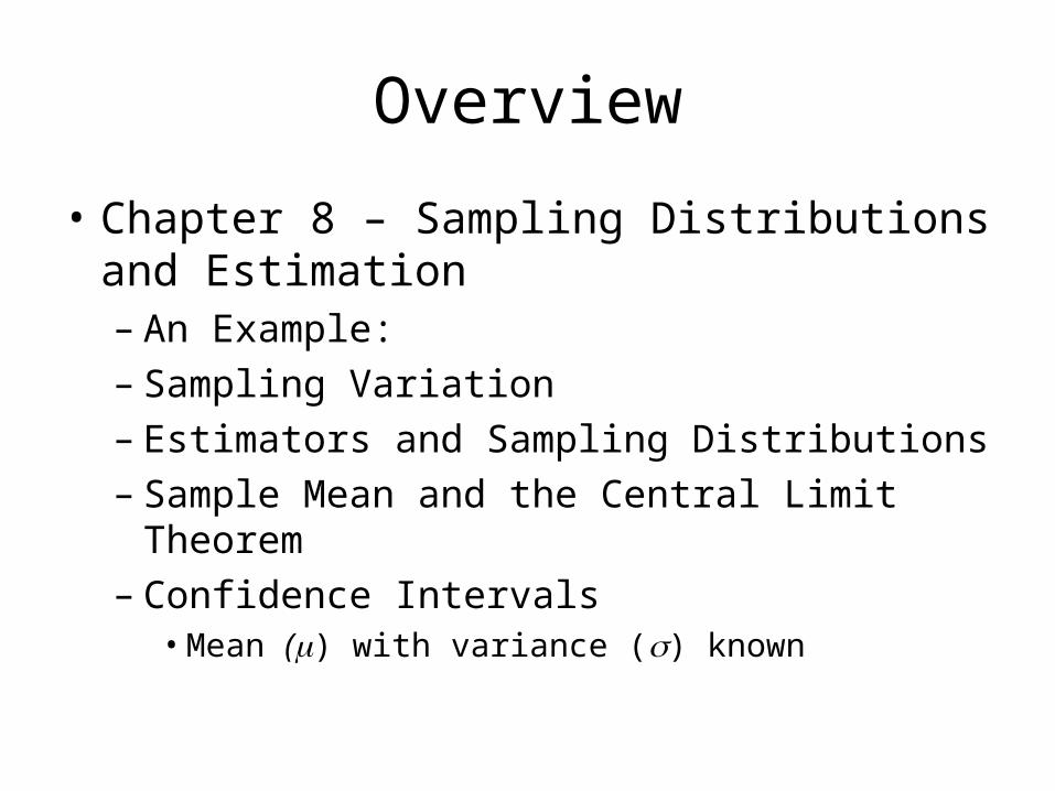
Overview

• Chapter 8 – Sampling Distributions and Estimation– An Example:– Sampling Variation– Estimators and Sampling Distributions– Sample Mean and the Central Limit Theorem– Confidence Intervals

• Mean () with variance () known

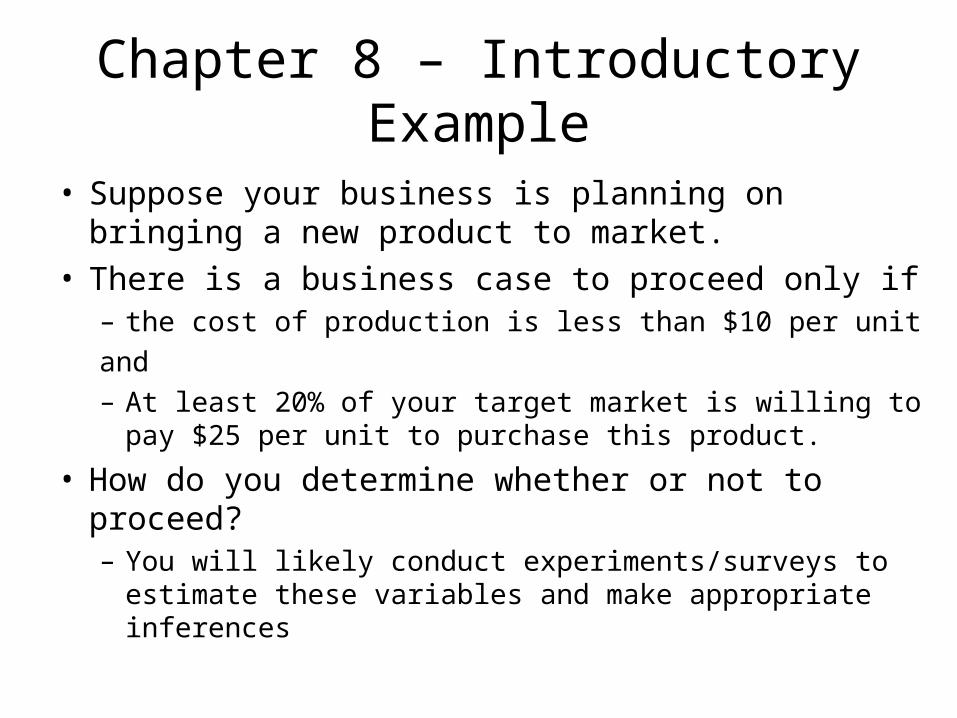
Chapter 8 – Introductory Example

• Suppose your business is planning on bringing a new product to market.

• There is a business case to proceed only if– the cost of production is less than $10 per unit

and– At least 20% of your target market is willing to pay $25

per unit to purchase this product.

• How do you determine whether or not to proceed?– You will likely conduct experiments/surveys to estimate

these variables and make appropriate inferences

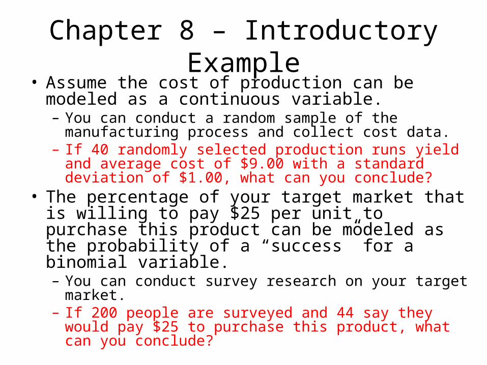
Chapter 8 – Introductory Example• Assume the cost of production can be modeled as

a continuous variable.– You can conduct a random sample of the

manufacturing process and collect cost data.– If 40 randomly selected production runs yield and

average cost of $9.00 with a standard deviation of $1.00, what can you conclude?

• The percentage of your target market that is willing to pay $25 per unit to purchase this product can be modeled as the probability of a “success” for a binomial variable.– You can conduct survey research on your target

market.– If 200 people are surveyed and 44 say they would pay

$25 to purchase this product, what can you conclude?

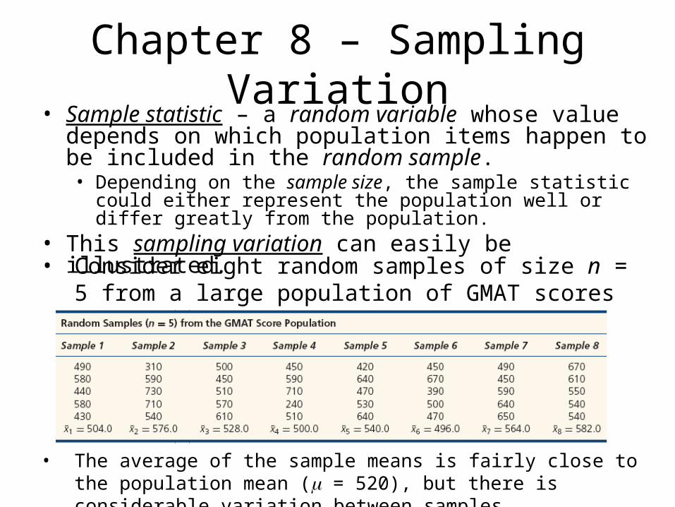
Chapter 8 – Sampling Variation• Sample statistic – a random variable whose value depends

on which population items happen to be included in the random sample.• Depending on the sample size, the sample statistic could either

represent the population well or differ greatly from the population.• This sampling variation can easily be illustrated.

• Consider eight random samples of size n = 5 from a large population of GMAT scores for MBA applicants.

• The average of the sample means is fairly close to the population mean ( = 520), but there is considerable variation between samples.

Chapter 8 – Estimators and Sampling Distributions

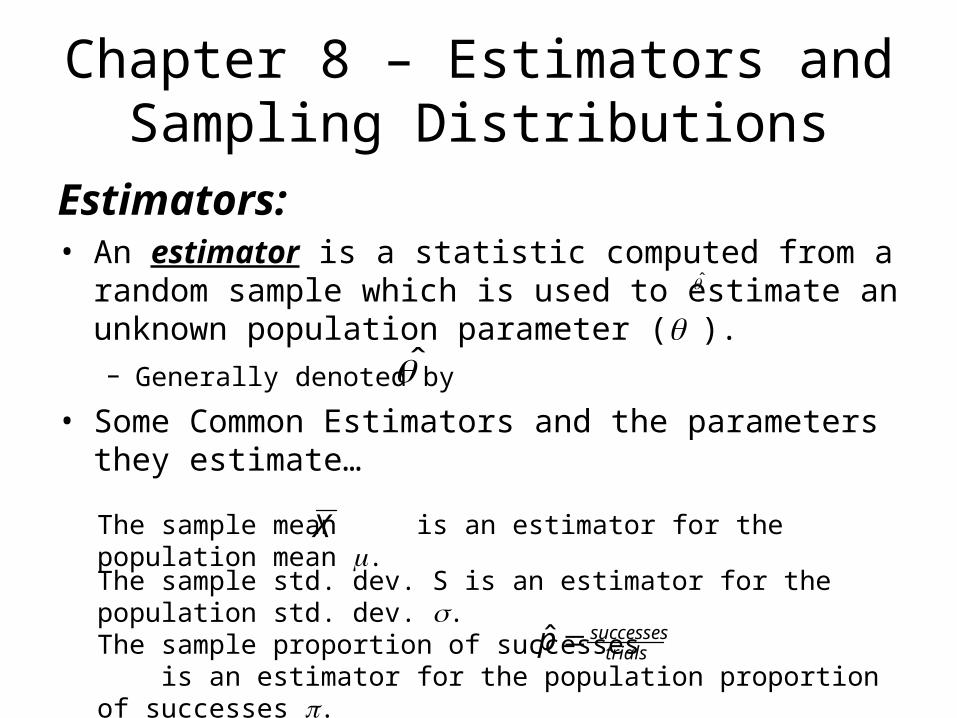
Estimators:• An estimator is a statistic computed from a random

sample which is used to estimate an unknown population parameter ().– Generally denoted by

• Some Common Estimators and the parameters they estimate…

The sample mean is an estimator for the population mean .X

The sample std. dev. S is an estimator for the population std. dev. .

The sample proportion of successes is an estimator for the population proportion of successes .

trialssuccessesp ˆ

Chapter 8 – Estimators and Sampling Distributions

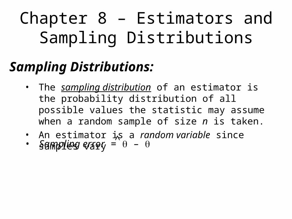
• The sampling distribution of an estimator is the probability distribution of all possible values the statistic may assume when a random sample of size n is taken.

• An estimator is a random variable since samples vary

Sampling Distributions:

• Sampling error = – ^

Chapter 8 – Estimators and Sampling Distributions

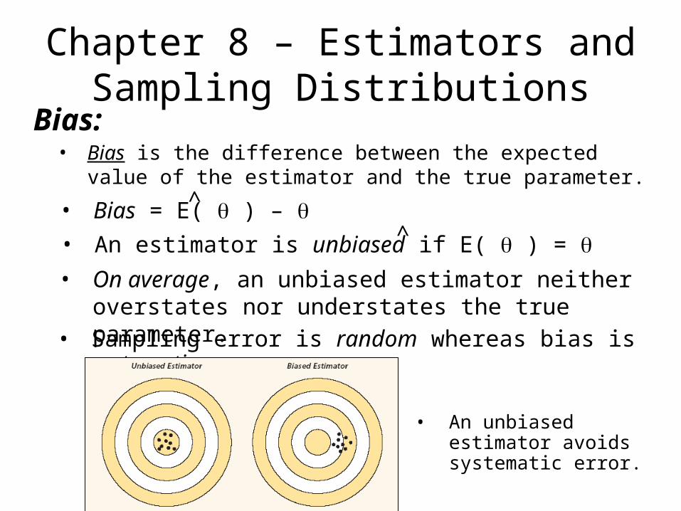
• Bias is the difference between the expected value of the estimator and the true parameter.

Bias:

• On average, an unbiased estimator neither overstates nor understates the true parameter.

• Bias = E( ) – ^

• An estimator is unbiased if E( ) = ^

• Sampling error is random whereas bias is systematic.

• An unbiased estimator avoids systematic error.

Chapter 8 – Estimators and Sampling Distributions

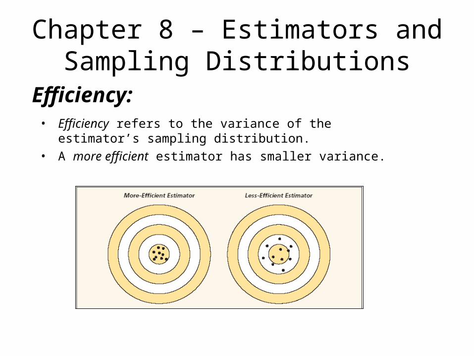
• Efficiency refers to the variance of the estimator’s sampling distribution.

• A more efficient estimator has smaller variance.

Efficiency:

Chapter 8 – Estimators and Sampling Distributions

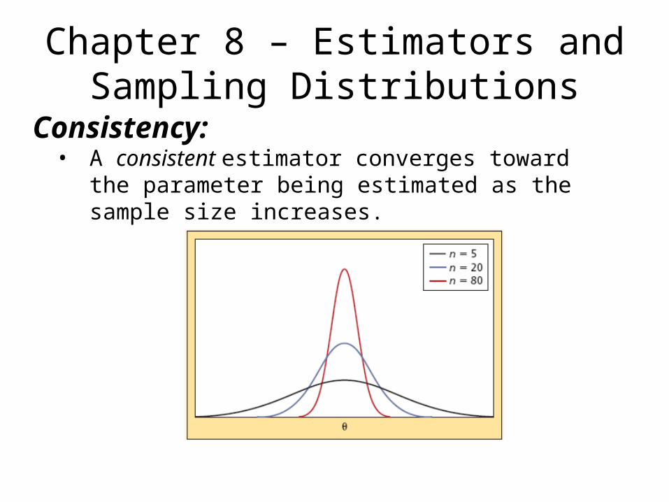
• A consistent estimator converges toward the parameter being estimated as the sample size increases.

Consistency:

Chapter 8 – Sample Mean and the Central Limit Theorem

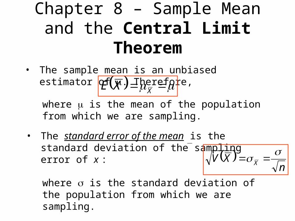
• The sample mean is an unbiased estimator of . Therefore,

• The standard error of the mean is the standard deviation of the sampling error of x :

where is the standard deviation of the population from which we are sampling.

where is the mean of the population from which we are sampling.

XXE

n

XV X

Chapter 8 – Sample Mean and the Central Limit Theorem

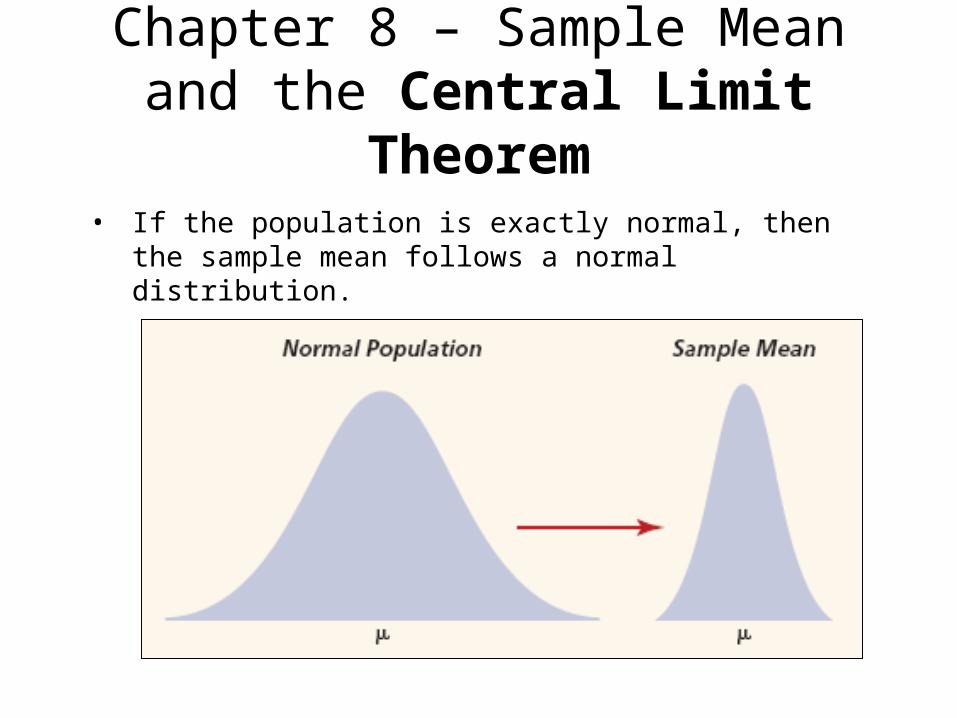
• If the population is exactly normal, then the sample mean follows a normal distribution.

Chapter 8 – Sample Mean and the Central Limit Theorem

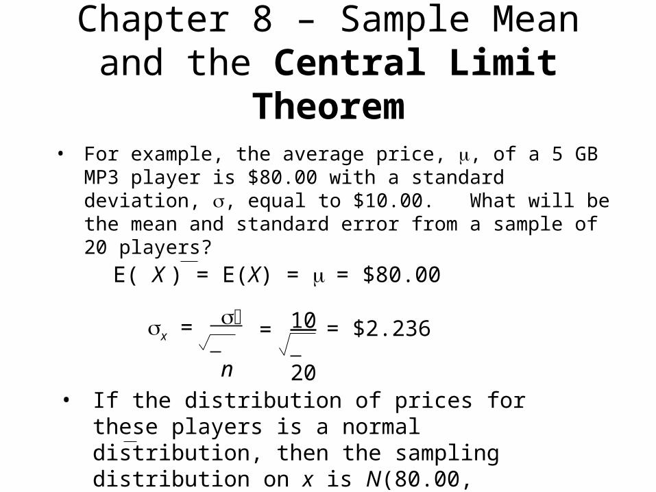
• For example, the average price, , of a 5 GB MP3 player is $80.00 with a standard deviation, , equal to $10.00. What will be the mean and standard error from a sample of 20 players?

E( X ) = E(X) = = $80.00

x = n

= 1020

= $2.236

• If the distribution of prices for these players is a normal distribution, then the sampling distribution on x is N(80.00, 2.236).

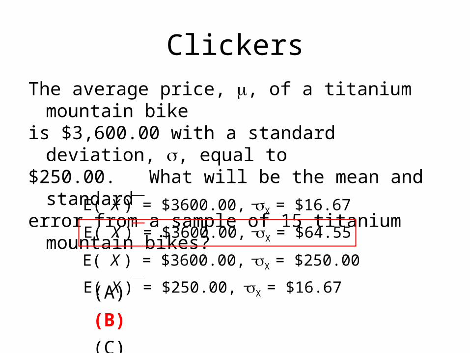
Clickers

The average price, , of a titanium mountain bike is $3,600.00 with a standard deviation, , equal to $250.00. What will be the mean and standard error from a sample of 15 titanium mountain bikes?

(A)

(B)

(C)

(D)E( X ) = $250.00, X = $16.67

E( X ) = $3600.00, X = $16.67

E( X ) = $3600.00, X = $64.55

E( X ) = $3600.00, X = $250.00

_

_

_

_

Chapter 8 – Sample Mean and the Central Limit Theorem

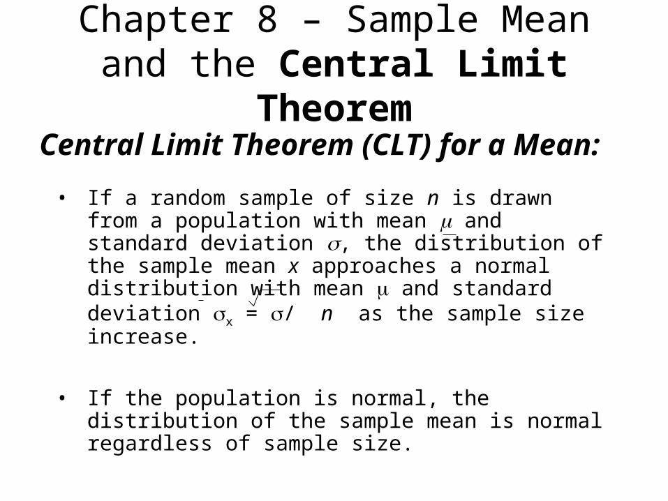
• If a random sample of size n is drawn from a population with mean and standard deviation , the distribution of the sample mean x approaches a normal distribution with mean and standard deviation x = / n as the sample size increase.

• If the population is normal, the distribution of the sample mean is normal regardless of sample size.

Central Limit Theorem (CLT) for a Mean:

Chapter 8 – Sample Mean and the Central Limit Theorem

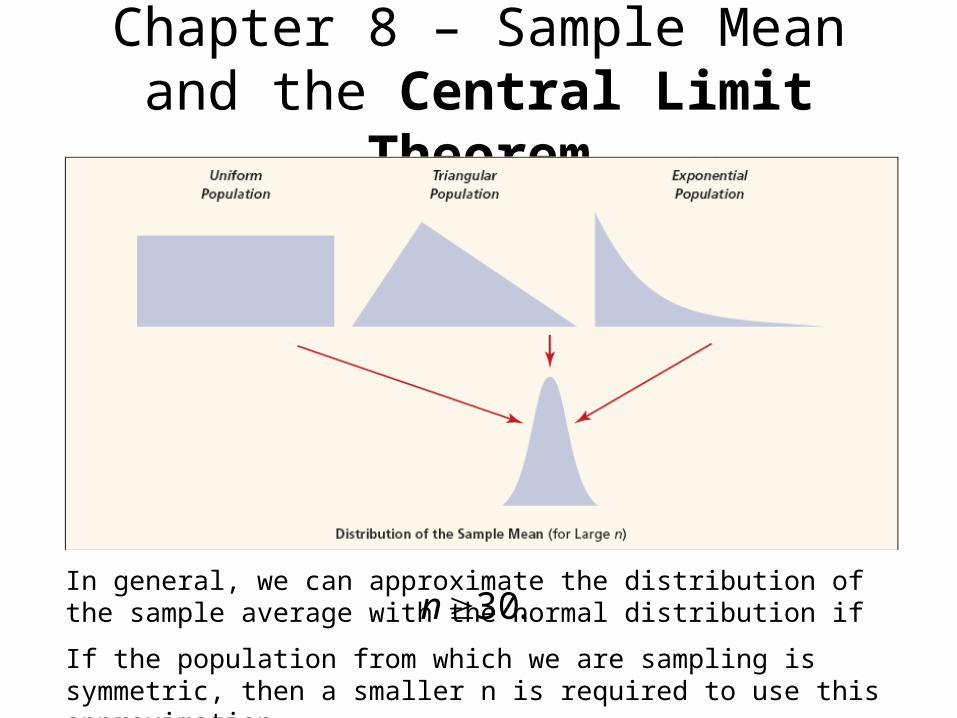
In general, we can approximate the distribution of the sample average with the normal distribution if .30nIf the population from which we are sampling is symmetric, then a smaller n is required to use this approximation.

Chapter 8 – Sample Mean and the Central Limit Theorem

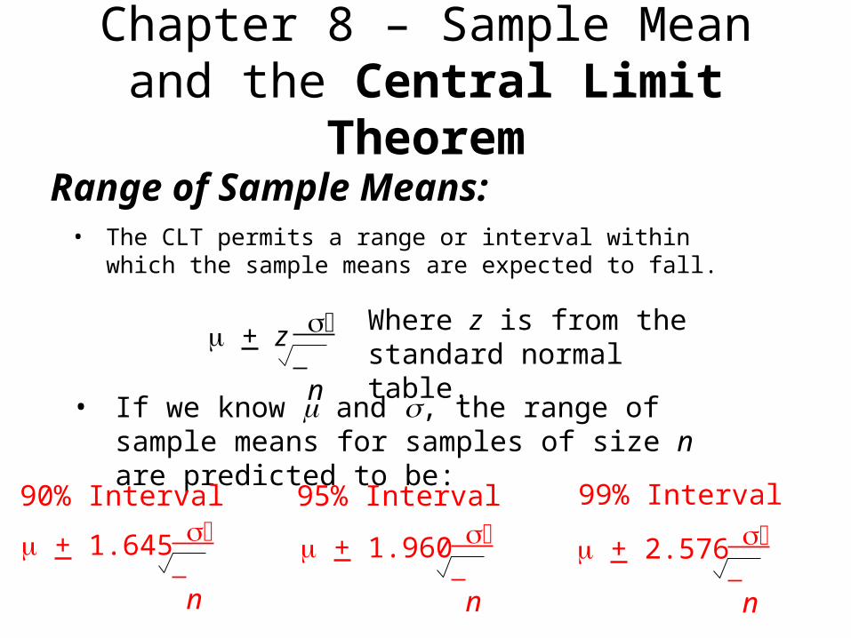
• The CLT permits a range or interval within which the sample means are expected to fall.

Range of Sample Means:

• If we know and , the range of sample means for samples of size n are predicted to be:

+ z n

Where z is from the standard normal table.

+ 1.645 n

90% Interval

+ 1.960 n

95% Interval

+ 2.576 n

99% Interval

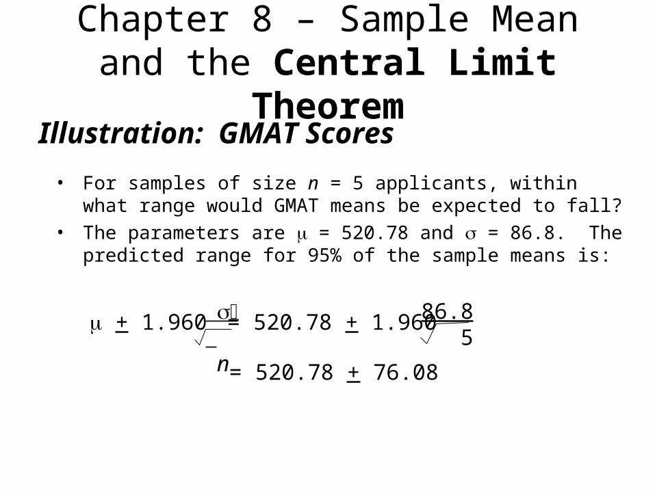
Chapter 8 – Sample Mean and the Central Limit Theorem

• For samples of size n = 5 applicants, within what range would GMAT means be expected to fall?

• The parameters are = 520.78 and = 86.8. The predicted range for 95% of the sample means is:

Illustration: GMAT Scores

+ 1.960 n

= 520.78 + 1.960 86.8 5

= 520.78 + 76.08

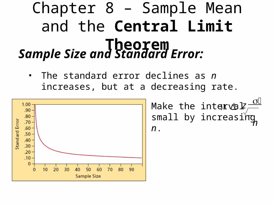
Chapter 8 – Sample Mean and the Central Limit Theorem

Make the intervalsmall by increasing n.

+ z n

• The standard error declines as n increases, but at a decreasing rate.

Sample Size and Standard Error:

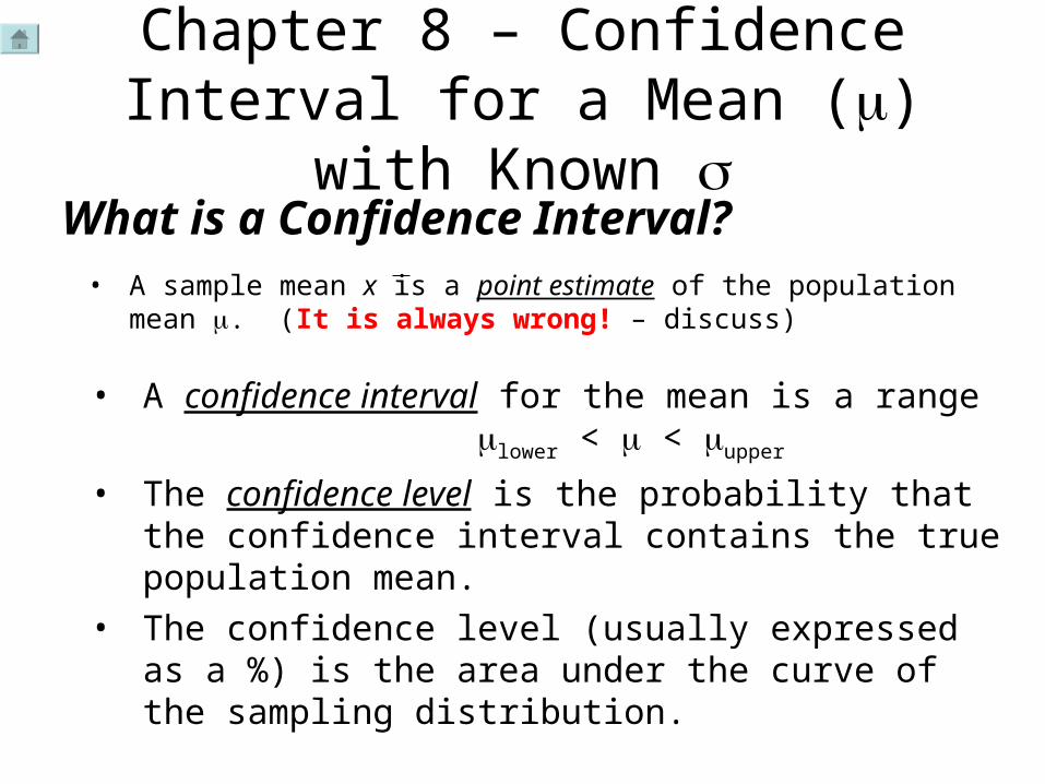
Chapter 8 – Confidence Interval for a Mean () with Known

• A sample mean x is a point estimate of the population mean . (It is always wrong! – discuss)

What is a Confidence Interval?

• A confidence interval for the mean is a range lower < < upper

• The confidence level is the probability that the confidence interval contains the true population mean.

• The confidence level (usually expressed as a %) is the area under the curve of the sampling distribution.

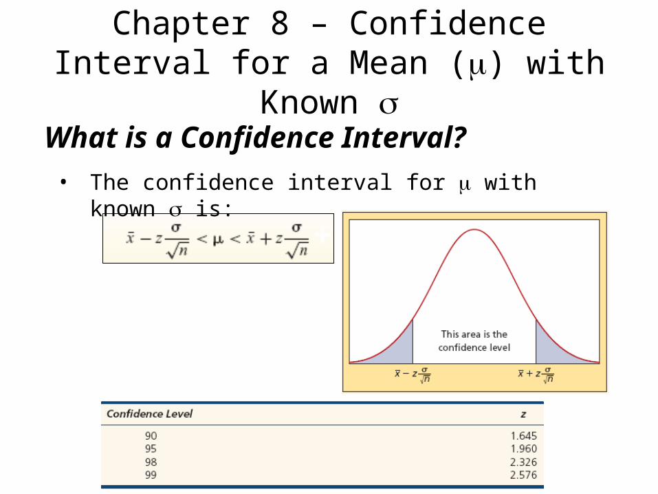
Chapter 8 – Confidence Interval for a Mean () with Known

What is a Confidence Interval?

• The confidence interval for with known is:

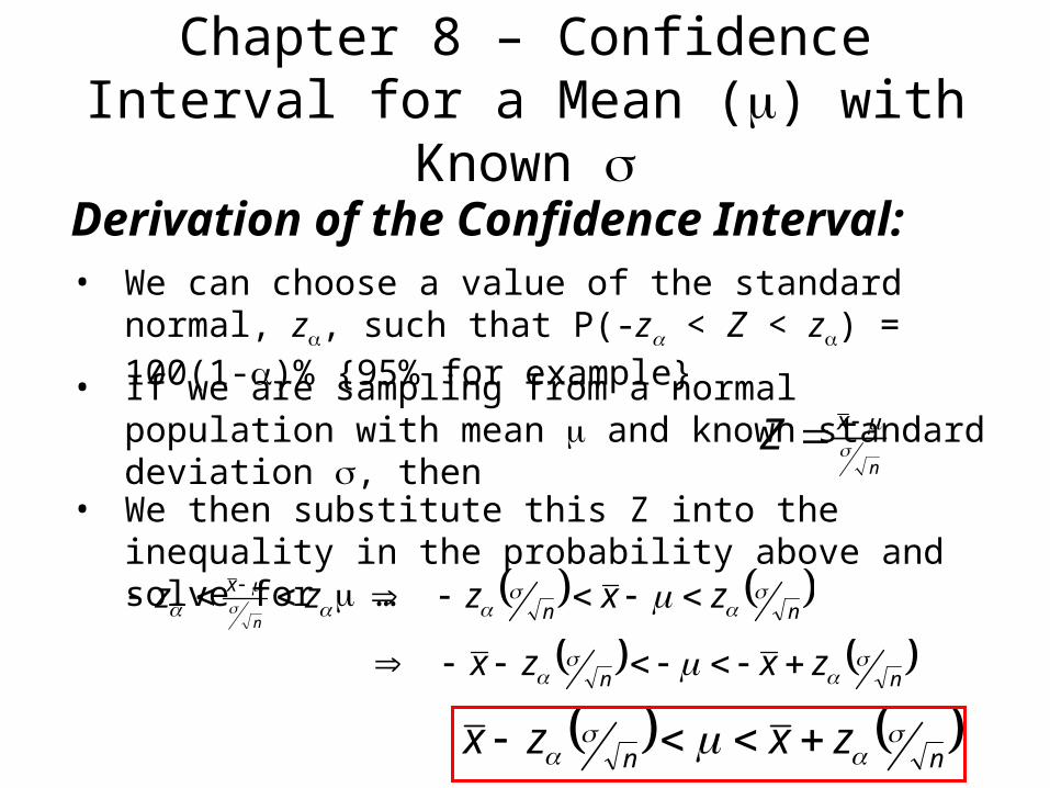
Chapter 8 – Confidence Interval for a Mean () with Known

n

xZ

nn

x zxzzzn

nn zxzx

Derivation of the Confidence Interval:• We can choose a value of the standard normal, z, such

that P(-z < Z < z) = 100(1-)% {95% for example}

• If we are sampling from a normal population with mean and known standard deviation , then

• We then substitute this Z into the inequality in the probability above and solve for …

nn zxzx

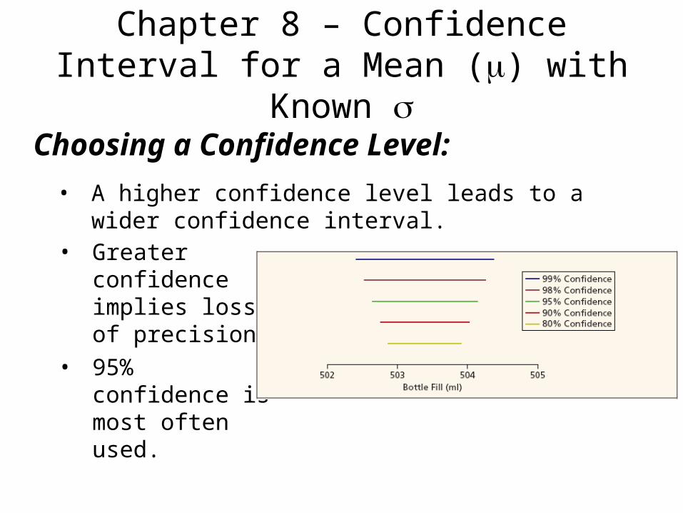
Chapter 8 – Confidence Interval for a Mean () with Known

• A higher confidence level leads to a wider confidence interval.

Choosing a Confidence Level:

• Greater confidence implies loss of precision.

• 95% confidence is most often used.

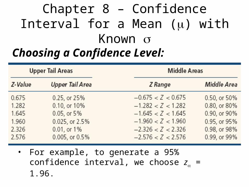
Chapter 8 – Confidence Interval for a Mean () with Known

Choosing a Confidence Level:

• For example, to generate a 95% confidence interval, we choose z = 1.96.

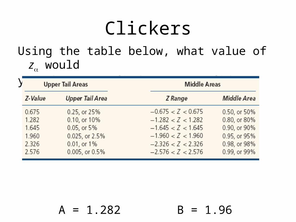
ClickersUsing the table below, what value of z would you choose to find a 99% confidence interval?

A = 1.282 B = 1.96

C = 2.326 D = 2.576

Chapter 8 – Confidence Interval for a Mean () with Known

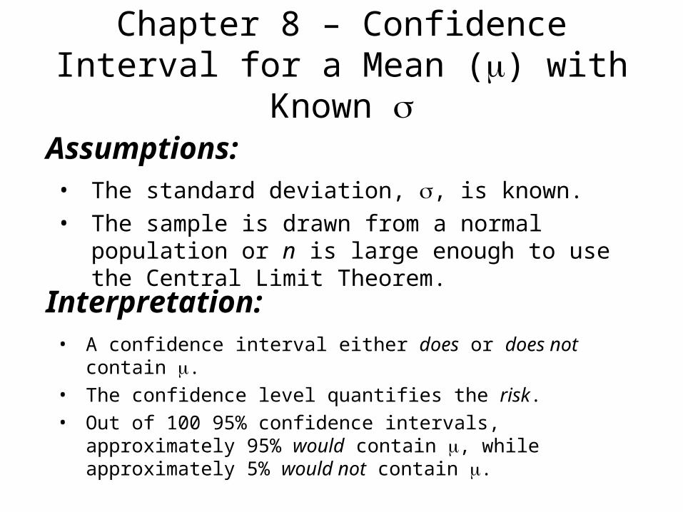
• A confidence interval either does or does not contain .• The confidence level quantifies the risk.• Out of 100 95% confidence intervals, approximately

95% would contain , while approximately 5% would not contain .

Interpretation:

• The standard deviation, , is known.• The sample is drawn from a normal population or n is

large enough to use the Central Limit Theorem.

Assumptions:

Chapter 8 – Confidence Interval for a Mean () with Known

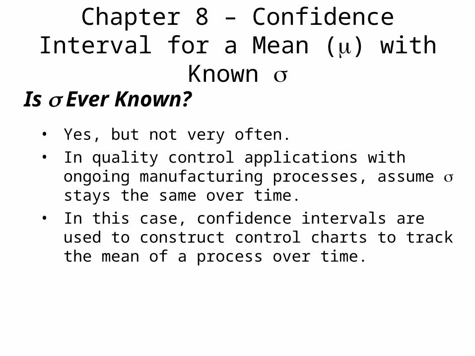
• Yes, but not very often.• In quality control applications with ongoing

manufacturing processes, assume stays the same over time.

• In this case, confidence intervals are used to construct control charts to track the mean of a process over time.

Is Ever Known?

Chapter 8 – Confidence Interval for a Mean () with Known

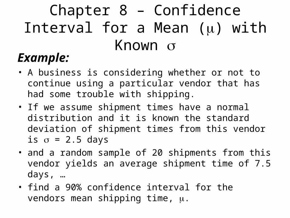
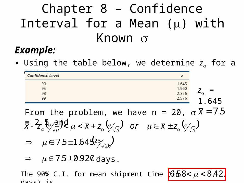
Example:• A business is considering whether or not to continue

using a particular vendor that has had some trouble with shipping.

• If we assume shipment times have a normal distribution and it is known the standard deviation of shipment times from this vendor is = 2.5 days

• and a random sample of 20 shipments from this vendor yields an average shipment time of 7.5 days, …

• find a 90% confidence interval for the vendors mean shipping time, .

Chapter 8 – Confidence Interval for a Mean () with Known

Example:• Using the table below, we determine z for a 90% C.I.

5.7x

z = 1.645

nnn zxorzxzx

20

5.2645.15.7

920.05.7

.42.858.6

From the problem, we have n = 20, = 2.5 and

days.

The 90% C.I. for mean shipment time (in days) is

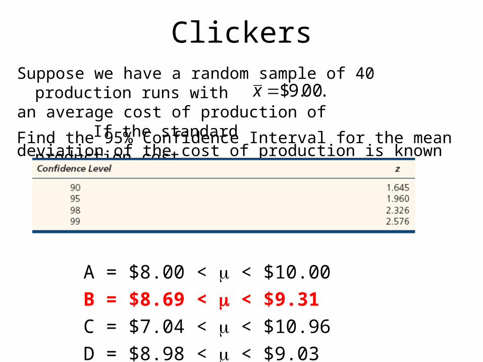
ClickersSuppose we have a random sample of 40 production runs with an average cost of production of If the standard deviation of the cost of production is known to be = $1.00,

Find the 95% Confidence Interval for the mean production cost.

A = $8.00 < < $10.00

B = $8.69 < < $9.31

C = $7.04 < < $10.96

D = $8.98 < < $9.03

.00.9$x