LLNL-CONF-483197

BayesLoc: A robust location program formultiple seismic events given animperfect earth model and error-corruptedseismic data

S. C. Myers, G. Johannesson, R. J. Mellors

May 9, 2011

Geothermal Resource CouncilSan Diego, CA, United StatesOctober 23, 2011 through October 26, 2011

Disclaimer

This document was prepared as an account of work sponsored by an agency of the United States government. Neither the United States government nor Lawrence Livermore National Security, LLC, nor any of their employees makes any warranty, expressed or implied, or assumes any legal liability or responsibility for the accuracy, completeness, or usefulness of any information, apparatus, product, or process disclosed, or represents that its use would not infringe privately owned rights. Reference herein to any specific commercial product, process, or service by trade name, trademark, manufacturer, or otherwise does not necessarily constitute or imply its endorsement, recommendation, or favoring by the United States government or Lawrence Livermore National Security, LLC. The views and opinions of authors expressed herein do not necessarily state or reflect those of the United States government or Lawrence Livermore National Security, LLC, and shall not be used for advertising or product endorsement purposes.

Paper for the GRC 2011 meetings.

Title: BayesLoc: A robust location program for multiple seismic events given an imperfect earth model and error-corrupted seismic data

Authors: Stephen C. Myers1, Gardar Johannesson1, and Robert J. Mellors1

1) Lawrence Livermore National Laboratory, 7000 East Ave, Livermore, CA 94550

Abstract

Accurate hypocentral locations of micro-earthquakes are essential for enhanced geothermal systems characterization and represent a first step for subsequent seismic analysis. Here we present an innovative location algorithm and software that provides robust locations and (Bayesian) estimates of the location error. Robustness to data error is highly useful for automated detection and location systems. Improved error estimates allow operators to reliably image fracture geometry with a precise understanding of the true spatial resolution (i.e. determine whether a “cloud” of seismicity truly represents a diffuse fracture network or is simply an artifact of location error). The probabilistic error estimates also provide a solid basis for risk assessments based on inferred fracture geometry.

The problem of locating seismic activity (3-dimensional position and time, i.e. the hypocenter) has a long history in the seismic community. The location problem itself can be stated as a relatively simple inversion: find the hypocenter that minimizes the difference between the observed and predicted arrival times of seismic phases at a network of seismic instruments. Complicating factors include: (1) the predicted arrival-times are imperfect, due to an imperfect earth model, (2) the observed arrival-times are subject to measurement error, and (3) the data set of arrival times can be corrupted by phase labeling and instrument timing errors. The fact that geographic network coverage is commonly not ideal compounds the effect of data errors, leading to inaccurate locations. Most troubling, estimates of location uncertainty are commonly not representative of true location error, because most location methods only account for Gaussian measurement errors.

Existing location methods fall broadly into two categories: those that locate one event at a time (single-event methods) and those that locate multiple events simultaneously (multiple-event methods). Multiple-event locators are superior to the single-event locators, as they can leverage the information available in the whole data set to mitigate and/or account for the impact of data and model errors. Nonetheless, existing multiple-event location results are notoriously subject to systematic biases due to an imperfect travel-time model, and multiple-event methods can be very sensitive to data set corruption.

We have developed BayesLoc: a robust multiple-event locator that improves on existing multiple-event locators, both in terms of robustness and accuracy. The locator is probabilistic (Bayesian) and simultaneously provides a probabilistic characterization of the unknown origin parameters, corrections to the assumed travel-time model, the precision of the observed arrival-time data, and accuracy of the assigned phase labels (including identifying outliers). Inference on the joint posterior probability distribution of all the parameters that define the multiple-event location problem is carried out using a Markov Chain Monte Carlo (MCMC) sampler. The end result is not just a single estimate of the location of each event, but a sample (a collection of posterior realizations) of locations that are consistent with the observed arrival-time data, to the degree of fidelity required by the precision of the data and the correctness of the travel-time model. This provides consistent location estimates with representative “error bars” (e.g., 90% probability regions), along with information about the correctness of the assumed travel-time model and the accuracy of the arrival-time data. Bayesloc has been successfully used to accurately locate event datasets containing tens to thousands of events, from small clusters to globally distributed events. In both cases location accuracy and uncertainty estimates have been validated using ground-truth events.

In this paper we present the probabilistic approach at the core of Bayesloc, how sampling-based posterior inference is carried out given observed arrival-time data, case studies at regional and global scales, and discuss application of Bayesloc at local distances and settings typical of geothermal reservoirs.

Introduction

Accurate location of micro-seismic activity in geothermal fields informs estimates of in-situ fracturing that occurs during fluid injection and enhanced stimulation activities (e.g. Albright and Pearson, 1982; House, 1987). Single-event location methods generally result in a cloud of seismic locations. Unfortunately, scatter in seismic locations is thought to be the result of location errors, providing little insight into the fracture geometry (e.g. Fehler et al., 2001). Event locations based on precise waveform correlation picks, careful analyst review, and multiple-event location methods can reveal detailed structure of fracture networks (e.g. Rutledge and Phillips, 2003), but meticulous data culling is required. Unrealistic uncertainty estimates of location results are a further shortcoming of current multiple-event methods, which use linearized solvers. Formal uncertainties for linearized inversion methods notoriously under estimate the actual errors, which can result in inaccurate assessment of the true fracture geometry.

We are adapting the Bayesloc multiple-event location algorithm (Myers et al., 2007, 2009) for application to geothermal monitoring. Bayesloc is a joint probability function of the multiple-event location system that allows stochastic prior constraints on locations, data uncertainty, and travel time predictions. A stochastic, non-linear solver is used that properly propagates uncertainty throughout the multiple-event system and produces non-parametric uncertainty estimates. Bayesloc was initially developed for use with regional (event-station distances to 2000 km) and global monitoring networks, and extensive validation has confirmed improved location

accuracy and representative uncertainty estimates for event locations. Here we outline existing location methodologies, the Bayesloc method, and our plan for modifying Bayesloc for optimal application to geothermal data sets.

Seismic Event Location

The vast majority of methods for estimating hypocenter parameters are based on minimizing the difference between observed and predicted arrival times of seismic phases (residuals hereafter). Efficient minimization of residuals has traditionally involved iterating the solution to a linear system of equations to convergence (Geiger, 1912). While numerous strategies to address local minima and variable data quality have been introduced since the introduction of Geiger’s method, the fundamental method remains the same.

If Geiger’s method is used, then hypocenter uncertainties are estimated by scaling the partial derivatives at the optimal hypocenter by either data misfit (confidence region; Flinn, 1962) or by prior estimates for pick and/or travel time prediction error (coverage region; Evernden, 1969). Both confidence and coverage regions use Gaussian parameterization of uncertainty, which results in a 4-dimensional ellipsoid.

Non-linearity in the relationship between residuals and the event location increases when the horizontal distance to the stations of the seismic network is within a few multiples of the event depth, which is typically the case for geothermal characterization. Depending on the velocity structure and the network configuration, local minima may result in Geiger’s method converging to an erroneous hypocenter (local minimum), and the shape of the hypocenter uncertainty volume can deviate significantly from the Gaussian ellipsoid. Grid-search and stochastic solvers (e.g. Rodi, 2006; Lomax et al., 2000) are less susceptible to local minima and these methods lend themselves to non-Gaussian probability regions. These methods are also better suited for use with a 3-dimensional seismic model, because they do not require partial derivatives, which can be discontinuous and multi-valued in a complicated seismic velocity field.

Multiple-Event Location

The introduction of the multiple-event location technique (Douglas, 1967) brought impressive hypocenter precision to event clusters that are recorded on a common network. In addition to the expansion of the linear system of equations to include hypocenter parameters, partial derivatives, and residuals for many events, multiple-event formulations also include station-specific travel time corrections. Travel time corrections mitigate errors in the travel time predictions that are used to compute residuals, which improve the precision of hypocenter estimates. However, a loss of accuracy – manifested as a consistent and potentially large bias for all locations – is well documented (Douglas, 1967; Jordan and Sverdrup, 1981; Pavlis and Booker, 1983). If the location of one event is known, then accurate locations can be determined by locating relative to the master event (Dewey, 1972). However, master-event methods assume that the fixed hypocenter is perfectly known and that travel time prediction errors for all events and phases are the same (or highly correlated) at each of the network stations. These conditions are only met when a

calibration shot is used and seismic ray paths from all events to all stations are similar to ray paths for the master event. This is why early multiple-event methods are limited to event clusters.

In order to locate over broader geographic areas, Waldhauser and Ellsworth (2000) extend the residual differencing method (double difference, Got et al., 1994) for application to large geographic areas. For a continuous chain of seismicity the relative-location precision may be bootstrapped through the entire data set to attain high precision over the length of the chain. Waldhauser and Ellsworth (2000) use arrival-times based on waveform correlation to achieve measurement precision that can exceed the digital sampling level. However, even waveform-based picks require data culling to remove outliers that stem from spurious correlations, cycle skipping,clock errors and other data issues.

Bayesian Hierarchical Multiple-Event Locator (Bayesloc)

Bayesloc (Myers et al., 2007, 2009) is a formulation of the joint probability function that includes:1. event origins times (o), 2. travel times (T),

a. Earth-model-based travel times (F), b. plus corrections (),

3. arrival-time measurement (pick) precisions (), and 4. phase labels (W).

All of these parameters are estimated using the observed arrival times (a) and input phase labels (w). Using Bayes’ theorem, the overarching statistical model is

(1)

Equation 1 decomposes the inversion of arrival times and phase-label data to determine thecomponents of the multiple-event system (left-hand side of equation 1), into a collection of “forward” problems and prior constraints (right-hand side of equation 1). Specifically, the first term (right-hand side) computes the probability of observing the collection of arrivals given a set of hypocenters, travel times, phase labels, and pick precisions. The second term computes the probability of all travel times, given a model-based prediction (event location is implicit) and a collection of correction parameters. The third, fourth, fifth, and sixth terms are prior constraints on hypocenters, arrival-time measurement precisions, travel time correction parameters, and input phase labels, respectively. The denominator is the probability over all arrival data. We note that equation 1 is a general statistical formulation and each of the terms may be specified in a number of ways. For example, any Earth model can be used to compute the uncorrected travel time (F(x)), and the formulation of travel time corrections () can take many forms. Specification of each term in equation 1 is provided in Myers et al. (2007, 2009), and a summary is provided here.

Arrival time measurement precision (1/variance) is decomposed into phase, station, event, and cross terms (e.g. station-phase). Resolution of the full set of precision parameters is dependant on the data set, so selection of precision terms is tailored to the data set. For geothermal applications we expect the datum-specific measurement precision to take the follow from.

(2)

)(/)|()()(),()),(|)((),,,|(),|,,,,,(

apwWpppoxpxFxTpWToapwaWTxop

(VijW )1 ijW Wph i

ev jst wj

phase st

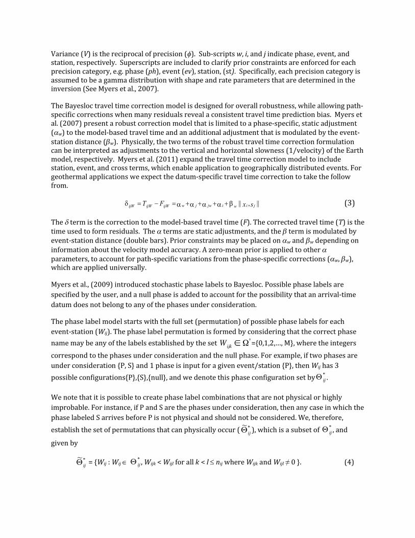
Variance (V) is the reciprocal of precision (). Sub-scripts w, i, and j indicate phase, event, and station, respectively. Superscripts are included to clarify prior constraints are enforced for each precision category, e.g. phase (ph), event (ev), station, (st). Specifically, each precision category is assumed to be a gamma distribution with shape and rate parameters that are determined in the inversion (See Myers et al., 2007).

The Bayesloc travel time correction model is designed for overall robustness, while allowing path-specific corrections when many residuals reveal a consistent travel time prediction bias. Myers et al. (2007) present a robust correction model that is limited to a phase-specific, static adjustment (w) to the model-based travel time and an additional adjustment that is modulated by the event-station distance (w). Physically, the two terms of the robust travel time correction formulation can be interpreted as adjustments to the vertical and horizontal slowness (1/velocity) of the Earth model, respectively. Myers et al. (2011) expand the travel time correction model to include station, event, and cross terms, which enable application to geographically distributed events. For geothermal applications we expect the datum-specific travel time correction to take the follow from.

(3)

The term is the correction to the model-based travel time (F). The corrected travel time (T) is the time used to form residuals. The terms are static adjustments, and the term is modulated by event-station distance (double bars). Prior constraints may be placed on w and w depending on information about the velocity model accuracy. A zero-mean prior is applied to other parameters, to account for path-specific variations from the phase-specific corrections (w, w), which are applied universally.

Myers et al., (2009) introduced stochastic phase labels to Bayesloc. Possible phase labels are specified by the user, and a null phase is added to account for the possibility that an arrival-time datum does not belong to any of the phases under consideration.

The phase label model starts with the full set (permutation) of possible phase labels for each event-station (Wij). The phase label permutation is formed by considering that the correct phase name may be any of the labels established by the set ={0,1,2,…, M}, where the integers correspond to the phases under consideration and the null phase. For example, if two phases are under consideration {P, S} and 1 phase is input for a given event/station {P}, then Wij has 3 possible configurations{P},{S},{null}, and we denote this phase configuration set by .

We note that it is possible to create phase label combinations that are not physical or highly improbable. For instance, if P and S are the phases under consideration, then any case in which the phase labeled S arrives before P is not physical and should not be considered. We, therefore, establish the set of permutations that can physically occur ( ), which is a subset of , and given by

= {Wij : Wij , Wijk < Wijl for all k < l nij where Wijk and Wijl ≠ 0 }. (4)

ijW TijW FijW w j jw i w || ix , js ||

*ij

*~ij *

ij

*~ij *

ij

Equation 4 states that the elements of are comprised of combinations of Wij such that the arrival time order of the phase labels is established a priori and the order given by ij, with the phase labeled as 1 arriving before 2, 2 before 3, etc. The null phase label is exempt from arrival time order constraint.

A priori phase-label probability is determined jointly for each set of event/station observations Wij.

(5)

where Zij is a normalizing constant and fijk is the prior probability of a given phase label conditional on the input phase label. We see from equation 5 that the probability of any phase configuration Wij is computed by multiplying the marginal probabilities of the individual members of the set Wij

and normalizing across all viable possibilities. Note that the probability is zero if the set Wij

violates the a priori arrival-time order.

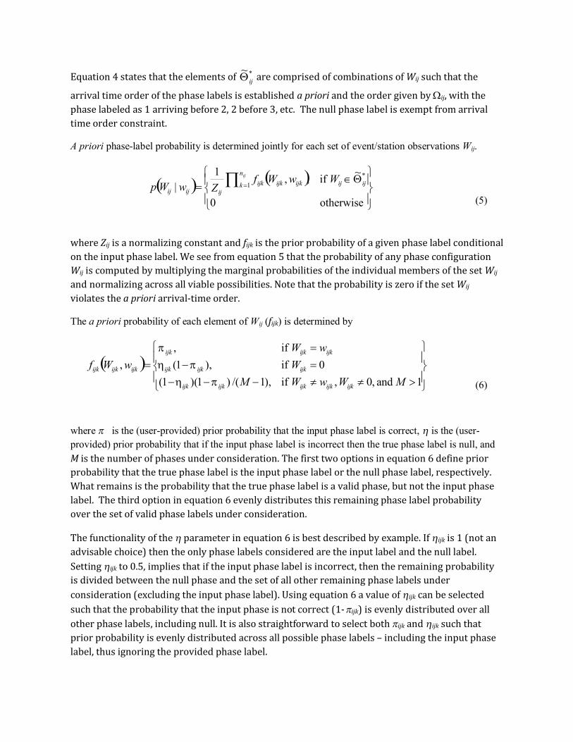
The a priori probability of each element of Wij (fijk) is determined by

(6)

where is the (user-provided) prior probability that the input phase label is correct, is the (user-provided) prior probability that if the input phase label is incorrect then the true phase label is null, and M is the number of phases under consideration. The first two options in equation 6 define prior probability that the true phase label is the input phase label or the null phase label, respectively. What remains is the probability that the true phase label is a valid phase, but not the input phase label. The third option in equation 6 evenly distributes this remaining phase label probability over the set of valid phase labels under consideration.

The functionality of the parameter in equation 6 is best described by example. If ijk is 1 (not an advisable choice) then the only phase labels considered are the input label and the null label. Setting ijk to 0.5, implies that if the input phase label is incorrect, then the remaining probability is divided between the null phase and the set of all other remaining phase labels under consideration (excluding the input phase label). Using equation 6 a value of ijk can be selected such that the probability that the input phase is not correct (1-ijk) is evenly distributed over all other phase labels, including null. It is also straightforward to select both ijk and ijk such that prior probability is evenly distributed across all possible phase labels – including the input phase label, thus ignoring the provided phase label.

*~ij

otherwise0

~if,,1|

*1 ijij

n

k ijkijkijkijijij

WwWfZwWp

ij

1and,0,if),1/()1)(1(

0if),1(if,

,MWwWM

WwW

wWf

ijkijkijkijkijk

ijkijkijk

ijkijkijk

ijkijkijk

Markov-Chain Monte Carlo (MCMC) Inversion

Using equation 1 allows the computation and comparison of the joint probability for two states of the multiple-event system, which enables application of the well-developed MCMC inversion methodology. In practice MCMC is used to generate realizations from the joint posterior distribution of all multiple-event model parameters; event locations, travel-time corrections, etc, and post-processing is used to summarize the samples by plotting point density or by averaging point populations to determine conventional hypocenter parameters. As the name implies, MCMC is Markovian in nature, and a new sample point (x*) is conditionally generated based upon the current sample point (x), using a transition kernel K(x, x*) determined by a specified target probability distribution p(x), which ultimately yields a chain of sample points; x1, x2, ..., xN (or samples) mentioned previously. A sufficient condition for the transition kernel to produce a sample from p(x) is that it satisfies the detailed balance condition, p(dx)K(x,dx*) = p(dx*)K(x*,dx) (e.g., Robert and Casella, 2004). The detailed balance condition stipulates that the chain has the same probability (density) of moving from x to x* as it does to move from x* to x. If the detailed balance condition is satisfied, the target distribution p(x) is invariant to the transition kernel K(x, x*), meaning that if x is known to be a valid realization from p(x), then x* sampled from K(x, x*) is also a valid realization from p(x). The detailed balance condition is the theoretical backbone of MCMC that ensures generation of valid samples from the distribution p(x). Because the starting configuration generally includes sampling from broad distributions on parameters for which little or no prior information is available, the influence of the starting values is reduced by discarding samples from an initial ‘burn-in’ period. Further details on the use of MCMC in Bayesian settings can be found in Tarantola (2004), Gelman, et al. (2004), and Robert and Casella (2004).

The Bayesloc hierarchical model lends itself to an efficient transition kernel. The simplest transition kernel, random samples for each model parameter, can be highly inefficient. A set of independent, random proposals for each parameter is likely to be jointly rejected based on low probability of equation 1. Therefore, we resort to random walk sampling only when absolutely necessary. The event locations themselves cannot be analytically derived from the other parameters, and therefore require random-walk sampling. However, the hierarchical approach promotes efficient realization of the remaining parameters (origin times, travel-time model parameters, and arrival-time precision parameters, and phase labels) by way of conditional sampling based upon a given configuration of event locations.

A single MCMC iteration is accomplished by first sampling each location using a Metropolis random walk (MRW), then progressively sampling additional parameters using either the Gibbs sampler (GS) (e.g. Gelman et al., 2004) or the slice sampler (SS) (e.g. Neil, 2003; Robert and Casella, 2004).

Examples

Testing in a geothermal setting is underway. As an example of the location improvement we show a case study of events with known locations at distances of several hundred km. This differs from typical geothermal field but the overall methodology will be similar. The data set includes 74 nuclear explosions with (for seismic location purposes) perfectly known hypocenters (Walter et al., 2004).

Figure 1 presents epicenter errors for 3 test cases: single-event location (Figure 1a), a multiple-event location algorithm that is similar to Jordan and Sverdrup (1983) (Figure 1b), and Bayesloc (Figure 1c). The single-event location results show considerable scatter with a mean

location error of 3.12 km. The Jordan and Sverdrup (1983) multiple-event location method results in precise relative locations, but all epicenters are biased. The bias causes a degradation of location accuracy compared to the single-event locations, with a mean epicenter error of 3.19 km. The Bayesloc locations (Figure 1c) are unbiased, due to Bayesloc’s robust travel time correction model, and the large location outliers are eliminated because inconsistent arr ival-time data are down weighted. The mean epicenter error for Bayesloc is 1.51 km.

Figure 1. Known epicenters and those determined using the iasp91 starting model and: a) a grid-search single event locator, b) a multiple-event locator similar to Jordan and Sverdrup (1981), c) Bayesloc. A line connects the known location (star) to the estimated epicenter in each test case (circle). Modified from Myers et al., 2009.

An example of the MCMC scatter plot of epicenter solutions and the associated point density is shown in Figure 2. The known location is plotted at the origin. Two distinct modes (regions of peaked sample density) are found. Linearized location algorithms would converge to either mode and the uncertainty estimate would – at best – represent the error of one mode. Bayesloc identifies that two modes exist, each with approximately equal probability. Figure 2b shows the hypocenter samples that are color coded by different phase configurations. The red samples comprise the western mode, which consists of the phase labels provided by the analyst. Bayesloc finds two alternative phase label configurations that comprise the eastern mode, and the eastern mode is in agreement with the known location.

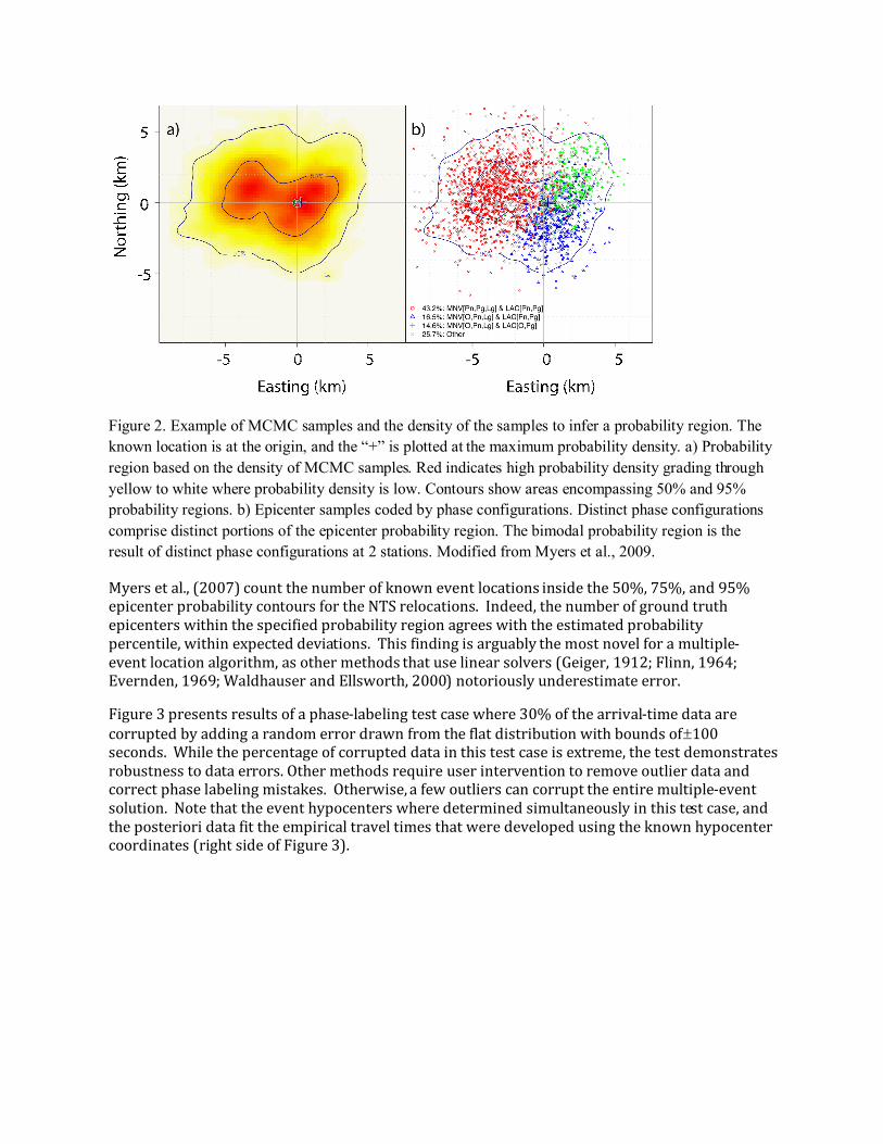
Figure 2. Example of MCMC samples and the density of the samples to infer a probability region. The known location is at the origin, and the “+” is plotted at the maximum probability density. a) Probability region based on the density of MCMC samples. Red indicates high probability density grading through yellow to white where probability density is low. Contours show areas encompassing 50% and 95% probability regions. b) Epicenter samples coded by phase configurations. Distinct phase configurations comprise distinct portions of the epicenter probability region. The bimodal probability region is the result of distinct phase configurations at 2 stations. Modified from Myers et al., 2009.

Myers et al., (2007) count the number of known event locations inside the 50%, 75%, and 95% epicenter probability contours for the NTS relocations. Indeed, the number of ground truth epicenters within the specified probability region agrees with the estimated probability percentile, within expected deviations. This finding is arguably the most novel for a multiple-event location algorithm, as other methods that use linear solvers (Geiger, 1912; Flinn, 1964; Evernden, 1969; Waldhauser and Ellsworth, 2000) notoriously underestimate error.

Figure 3 presents results of a phase-labeling test case where 30% of the arrival-time data are corrupted by adding a random error drawn from the flat distribution with bounds of 100 seconds. While the percentage of corrupted data in this test case is extreme, the test demonstrates robustness to data errors. Other methods require user intervention to remove outlier data and correct phase labeling mistakes. Otherwise, a few outliers can corrupt the entire multiple-event solution. Note that the event hypocenters where determined simultaneously in this test case, and the posteriori data fit the empirical travel times that were developed using the known hypocenter coordinates (right side of Figure 3).

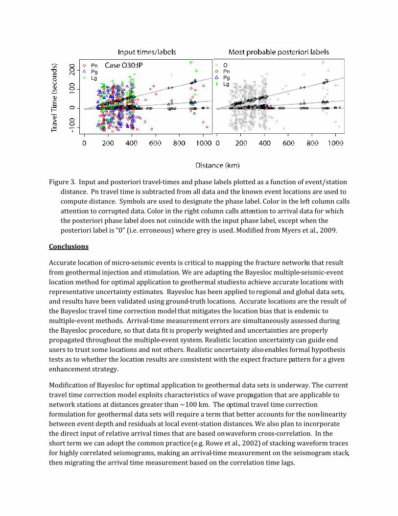
Figure 3. Input and posteriori travel-times and phase labels plotted as a function of event/station distance. Pn travel time is subtracted from all data and the known event locations are used to compute distance. Symbols are used to designate the phase label. Color in the left column calls attention to corrupted data. Color in the right column calls attention to arrival data for which the posteriori phase label does not coincide with the input phase label, except when the posteriori label is “0” (i.e. erroneous) where grey is used. Modified from Myers et al., 2009.

Conclusions

Accurate location of micro-seismic events is critical to mapping the fracture networks that result from geothermal injection and stimulation. We are adapting the Bayesloc multiple-seismic-event location method for optimal application to geothermal studiesto achieve accurate locations with representative uncertainty estimates. Bayesloc has been applied to regional and global data sets, and results have been validated using ground-truth locations. Accurate locations are the result of the Bayesloc travel time correction model that mitigates the location bias that is endemic to multiple-event methods. Arrival-time measurement errors are simultaneously assessed during the Bayesloc procedure, so that data fit is properly weighted and uncertainties are properly propagated throughout the multiple-event system. Realistic location uncertainty can guide end users to trust some locations and not others. Realistic uncertainty alsoenables formal hypothesis tests as to whether the location results are consistent with the expect fracture pattern for a given enhancement strategy.

Modification of Bayesloc for optimal application to geothermal data sets is underway. The current travel time correction model exploits characteristics of wave propagation that are applicable to network stations at distances greater than ~100 km. The optimal travel time correctionformulation for geothermal data sets will require a term that better accounts for the non-linearity between event depth and residuals at local event-station distances. We also plan to incorporate the direct input of relative arrival times that are based on waveform cross-correlation. In the short term we can adopt the common practice (e.g. Rowe et al., 2002) of stacking waveform traces for highly correlated seismograms, making an arrival-time measurement on the seismogram stack, then migrating the arrival time measurement based on the correlation time lags.

ReferencesAlbright, J. N., and Pearson, C. F., 1982, Acoustic emissions as a tool for hydraulic fracture location:

Experience at the Fenton Hill Hot Dry Rock site: Soc. Petro. Eng. J., 22, August, 523–530.Douglas, A. (1967). Joint epicentre determination, Nature 215 47-48.Dewey, J.W., (1972). Seismicity and tectonics of western Venezuela, Bull. Seismol. Soc. Am, 62:

1711-1751.Evernden, J.F. (1969). Precision of Epicenters Obtained by Small Numbers of World-Wide Stations,

Bull. Seism. Soc. Am. 59 1365-1398.Fehler, M., Jupe, A., and Asanuma, H. (2001). More than cloud: New techniques for characterizing

reservoir structures using induced seismicity: The Leading Edge, 20, 324–328.Flinn, E.A. (1965). Confidence regions and error determinations for seismic event location, Rev.

Geophys. 3 157-185.Geiger, L. (1912). Probability method for the determination of earthquake epicenters from the

arrival time only (translated from Geiger's 1910 German article), Bulletin of St. Louis University, 8(1), 56-71.

Got, J.-L., J. Fréchet, and F. W. Klein (1994). Deep fault plane geometry inferred from multiplet relative relocation beneath the south flank of Kilauea, J. Geophys. Res. 99, 15,375–15,386.

House, L. (1987). Locating microearthquakes induced by hydraulic fracturing in crystalline rock: Geophys. Res. Lett., 14, 919–921.

Jordan, T.H., and K.A. Sverdrup (1981). Teleseismic location techniques and their application to earthquake clusters in the south-central Pacific, Bull. Seism. Soc. Am. 71 1105-1130.

Lomax, A., J. Virieux, P. Volant and C. Berge (2000). Probabilistic earthquake location in 3D and layered models: Introduction of a Metropolis-Gibbs method and comparison with linear locations, in Advances in Seismic Event Location Thurber, C.H., and N. Rabinowitz (eds.), Kluwer, Amsterdam, 101-134.

Myers, S.C., G. Johannesson, and W. Hanley (2007). A Bayesian hierarchical method for multiple-event seismic location, Geophys. J. Int., 171, 1049-1063.

Myers, S.C., G. Johannesson, and W. Hanley (2009). Incorporation of probabilistic seismic phase labels into a Bayesian multiple-event seismic locator, Geophys. J. Int., 177, 193-204.

Myers, S.C., G. Johannesson, and N.A. Simmons (2011). Global-scale P-wave tomography optimized for prediction of teleseismic and regional travel times for Middle East events: 1. Data set Development, Jour, Geophys. Res., 116, B04304, doi:10.1029/2010JB007967, 2011.=

Pavlis, G.L., and J.R. Booker (1983). Progressive multiple event location (PMEL), Bull. Seism. Soc. Am. 73 1753-1777.

Rodi, W. (2006). Grid-search event location with non-Gaussian error models, Phys. Earth Planet. In.158 55-66.

Rowe, C. A., Aster, R. C., Phillips, W. S., Jones, R. H., Borchers, B.,and Fehler, M. C. (2002). Using automated, high-precision repacking to improve delineation of microseismic structures at the Soultz geothermal reservoir: Pure Appl. Geophys., 159, 563–596.

Rutledge, J.T., and W.S. Phillips (2003). Hydraulic stimulation of natural fractures as revealed by induced microearthquakes, Carthage Cotton Valley gas field, east Texas, Geophysics, 68, No. 2, 441–452.

Waldhauser, F., and W. L. Ellsworth, (2000). A double-difference earthquake location algorithm: method and application to the Northern Hayward Fault, CA, Bull. Seism. Soc. Am. 90, 1353–1368.