bayesian model averaging and exchange rate forecasts

Journal of Econometrics 146 (2008) 329–341

Contents lists available at ScienceDirect

Journal of Econometrics

journal homepage: www.elsevier.com/locate/jeconom

Bayesian Model Averaging and exchange rate forecasts

Jonathan H. Wright ∗Department of Economics, Johns Hopkins University, 3400 North Charles Street, Baltimore, MD 21218, United States

a r t i c l e i n f o

Article history:Available online 28 August 2008

JEL classification:C32C53F31

Keywords:ShrinkageModel uncertaintyForecastingExchange ratesBootstrap

a b s t r a c t

Exchange rate forecasting is hard and the seminal result of Meese and Rogoff [Meese, R., Rogoff, K., 1983.Empirical exchange rate models of the seventies: Do they fit out of sample? Journal of InternationalEconomics 14, 3–24] that the exchange rate is well approximated by a driftless random walk, atleast for prediction purposes, still stands despite much effort at constructing other forecasting models.However, in several other macro and financial forecasting applications, researchers in recent yearshave considered methods for forecasting that effectively combine the information in a large number oftime series. In this paper, I apply one such method for pooling forecasts from several different models,Bayesian Model Averaging, to the problem of pseudo out-of-sample exchange rate predictions. Formost currency–horizon pairs, the Bayesian Model Averaging forecasts using a sufficiently high degreeof shrinkage, give slightly smaller out-of-sample mean square prediction error than the random walkbenchmark. The forecasts generated by this model averaging methodology are however very close to,but not identical to, those from the random walk forecast.

© 2008 Elsevier B.V. All rights reserved.

1. Introduction

Out-of-sample forecasting of exchange rates is hard. Meeseand Rogoff (1983) argued that all exchange rate models do lesswell in out-of-sample forecasting exercises than a simple driftlessrandom walk. Although this finding was heresy to many atthe time that Meese and Rogoff wrote their paper, it has nowbecome the conventional wisdom. Mark (1995) claimed that amonetary fundamentals model can generate better out-of-sampleforecasting performance at long horizons, but that result has beenfound to be very sensitive to the sample period (Groen, 1999; Faustet al., 2003). Claims that a particular variable has predictive powerfor exchange rates crop up frequently, but these results typicallyapply just to a particular exchange rate and a particular subsample.As such, they are by now met with justifiable skepticism and arethought of by many as the result of data-mining exercises.However, in many contexts, researchers have recently made

substantial progress in the econometrics of forecasting usinglarge datasets (i.e. a large number of predictors). The trick isto combine the information in these different variables in ajudicious way that avoids the estimation of a large number ofunrestricted parameters. Bayesian VARs have been found to beuseful in forecasting: these often usemany time series, but imposea prior that many of the coefficients in the VAR are close to zero.

∗ Tel.: +1 410 516 5728.E-mail address:[email protected].

0304-4076/$ – see front matter© 2008 Elsevier B.V. All rights reserved.doi:10.1016/j.jeconom.2008.08.012

Approaches in which the researcher estimates a small number offactors from a large dataset and forecasts using these estimatedfactors have also been shown to be capable of superior predictiveperformance (see for example Stock and Watson (2002) andBernanke and Boivin (2003)). Stock and Watson (2001, 2004)obtained good results in out-of-sample prediction of internationaloutput growth and inflation by taking forecasts from a largenumber of different simple models and just averaging them. Theyfound the good performance of simple model averaging to beremarkably consistent across subperiods and across countries. Thebasic idea that forecast combination outperforms any individualforecast is part of the folklore of economic forecasting, goingback to Bates and Granger (1969). It is of course crucial to theresult that the researcher just averages the forecasts (or takes amedian or trimmed mean). It is, in particular, tempting to runa forecast evaluation regression in which the weights on thedifferent forecasts are estimated as free parameters. While thisleads to a better in-sample fit, it gives less good out-of-sampleprediction.Bayesian Model Averaging (BMA) is another method for

forecasting with large datasets that has received considerablerecent attention in both the statistics and econometrics literature.The idea is to take forecasts from many different models, andto assume that one of them is the true model, but that theresearcher does not knowwhich this is. The researcher starts froma prior about which model is true and computes the posteriorprobabilities that eachmodel is the true one. The forecasts from allthe models are then weighted by these posterior probabilities. Ithas been used in a number of econometric applications, including

http://www.elsevier.com/locate/jeconom

http://www.elsevier.com/locate/jeconom

mailto:[email protected]

http://dx.doi.org/10.1016/j.jeconom.2008.08.012

330 J.H. Wright / Journal of Econometrics 146 (2008) 329–341

output growth forecasting (Min andZellner, 1993; Koop andPotter,2003), cross-country growth regressions (Doppelhofer et al., 2000;Fernandez et al., 2001) and stock return prediction (Avramov,2002; Cremers, 2002). Avarmov andCremers both report improvedpseudo-out-of-sample predictive performance from BMA.The contribution of this paper is to argue that BMA is useful for

out-of-sample forecasting of exchange rates in the last fifteen yearsalthough the magnitude of the improvement that it offers relativeto the random walk benchmark is quite small.One does not have to be a subjectivist Bayesian to believe

in the usefulness of BMA, or of Bayesian shrinkage techniquesmore generally. A frequentist econometrician can interpret thesemethods as pragmatic devices thatmaybeuseful for out-of-sampleforecasting in the face of model and parameter uncertainty.1 Theplan for the remainder of the paper is as follows. Section2describesthe idea of BMA. The out-of-sample exchange rate predictionexercise is described in Section 3. Section 4 concludes.

2. Bayesian model averaging

The idea of Bayesian Model Averaging was set out by Leamer(1978), and has recently received a lot of attention in the statisticsliterature, including in particular Raftery et al. (1997), Hoeting et al.(1999) and Chipman et al. (2001).Consider a set of nmodelsM1, . . . ,Mn. The ithmodel is indexed

by a parameter vector θi. The researcher knows that one of thesemodels is the true model, but does not know which one.2 Theresearcher has prior beliefs about the probability that the ithmodelis the true model which we write as P(Mi), observes data D, andupdates her beliefs to compute the posterior probability that theith model is the true model:

P(Mi|D) =P(D|Mi)P(Mi)n∑j=1P(D|Mj)P(Mj)

(1)

where

P(D|Mi) =∫P(D|θi,Mi)P(θi|Mi)dθ i (2)

is the marginal likelihood of the ith model, P(θi|Mi) is the priordensity of the parameter vector in this model and P(D|θi,Mi) is thelikelihood. Eachmodel implies a forecast. In the presence of modeluncertainty, our overall forecast weights each of these forecastsby the posterior for that model. This gives the minimum meansquare error forecast. The researcher needs only to specify theset of models, the model priors, P(Mi), and the parameter priors,P(θi|Mi).3The models do not have to be linear regression models, but I

shall henceforth assume that they are. The ithmodel then specifiesthat

y = Xiβi + ε (3)

1 For recent work considering frequentist approaches to model averaging, seeHjort and Claeskens (2003).2 For recent work considering Bayesian Model Averaging when none of the

models is in fact true, see Key et al. (1998) and Fernández-Villaverde and Rubio-Ramírez (2004). The BayesianModel Averaging procedure is consistent in the sensethat the weight on the model that is best in the Kullback–Leibler metric (which isthe true model if that exists, but is still well defined if none of the models is true)goes to one asymptotically as the sample size increases.3 The distinction between model uncertainty and parameter uncertainty is a

little artificial in the sense that one could write all the models as nested by asufficiently general model, and, within this nesting model, the only uncertaintyis then parameter uncertainty. The BMA approach would however imply veryparticular and rather peculiar priors for these parameters.

where y is a T × 1 vector of observations on a variable that theresearcher wishes to forecast, Xi is a T × pi matrix of predictors,βi is a pi × 1 parameter vector, ε is the disturbance vector,the disturbances are i.i.d. with mean zero and variance σ 2, andθi = (β ′i , σ

2). To obtain a closed form expression for the modellikelihood, I assume that the regressors are strictly exogenous. Thisassumption is clearly false in the application that I am consideringin this paper, but many methods for combining a large number ofvariables in forecasting exercises (including bagging and empiricalBayes methods) likewise have a theoretical justification that relieson strict exogeneity of the regressors. And, any of these methodsmay still have good forecasting power even if the premise of strictexogeneity underlying their theoretical justification is false (seeStock and Watson (2005)). In this spirit, the goal of this paper issimply to assess the power of BMA in forecasting exchange rates.For the parameter priors, I shall take the natural conjugate g-

prior specification for βi, so that the prior for βi conditional onσ 2 is N(0, σ 2(X ′i Xi)

−1). For σ 2, I assume the improper prior thatis proportional to 1/σ 2. It is well known (see, for example, Zellner(1971)) that one can then calculate the required likelihood of themodel analytically as:

p(D|Mi) =12Γ (T/2)π T/2

(1+ ϕ)−pi/2S−Ti (4)

where S2i = Y′Y − Y ′Xi(X ′i Xi)

−1X ′i Yϕ

1+ϕ , while the posterior meanfor βi is

βi = E(βi|D,Mi) =ϕ

ϕ + 1(X ′i Xi)

−1X ′i Y . (5)

The prior for βi is a proper prior. In BMA, one cannot useimproper priors for model-specific parameters, because improperpriors are unique only up to an arbitrary multiplicative constantand so their use would lead to an indeterminacy of the modelposterior probabilities (Kass and Raftery, 1995). Besides, I want tohave an informative prior for βi. The prior for βi is centered aroundzero and so each model is shrunk towards a lack of forecastability.The extent of this shrinkage is governed by ϕ. A smaller value of ϕmeans more shrinkage and makes the prior more informative, butthis may help in out-of-sample forecasting. Researchers often tryto make the prior as uninformative as possible, but at least in theexchange rate forecasting problemconsidered in this paper, amoreinformative prior turns out to give better predictive performance.One way of thinking about the role of ϕ is that it controls therelative weight of the data and our prior beliefs in computing theposterior probabilities of differentmodels. Ifϕ = 0, then P(D|Mi) isequal for all models and so the posterior probability of each modelbeing true is equal to the prior probability. The larger isϕ, themorewe are willing to move away from the model priors in responseto what we observe in the data. The prior for σ 2 is an inverse-gamma (0,0) prior, and is improper. An improper prior can be usedfor σ 2, because this parameter is common to all models, and thusthe arbitrary multiplicative constant in this prior does not affectthe posterior probabilities for the different models.This parameter prior has been used by Fernandez et al. (2001)

and many others in the BMA literature.4 The model priors will bediscussed in the context of the application in Section 3.

4 Alternatively, a conjugate inverse-gamma (c0, d0) prior could have been usedfor σ 2 with c0 > 0 and d0 > 0. This is a proper prior, but has the disadvantage thatis not invariant under scale transformations. Moreover it seems appropriate to havea prior for σ 2 that is as uninformative as possible.

J.H. Wright / Journal of Econometrics 146 (2008) 329–341 331

3. Exchange rate forecasting

I consider prediction of the bilateral exchange value of theCanadian dollar, pound, yen and mark/euro, relative to theUS dollar, using both direct forecasting and iterated multistepforecasting. Iterated forecasts are more efficient if the model iscorrectly specified, but direct forecasts may be more robust tomodel misspecification (see Marcellino et al. (2006)).

3.1. Direct forecasts

Turning first to direct forecasts, the ith model for forecastingexchange rates that I consider is of the form

et+h − et = β ′iX i,t + εt (6)where et denotes the log exchange rate (foreign currency perdollar), h is the forecasting horizon, Xi,t is the vector of regressorsin time period t for model i, and εt is the error term. Each modelimplies a forecast β ′iXi,t where βi denotes the posterior meanof βi. The proposed overall forecast then weights each of thesemodels by their posterior probabilities, so that the forecast is∑ni=1 P(Mi|D)β

′

iXi,t .Themodels will consist of all possible permutations of a set of λ

potential predictor variables, including all of these predictors andnone of them, making a total of 2λ candidate models. Each of thesemodels will also include a constant, except for the model with nopredictor variables at all which is simply the driftless randomwalket+h − et = εt . (7)Following Cremers (2002) and Koop and Potter (2003), among

others, I specify that the prior probability for any model with κpredictors (excluding any intercept) is

P(Mi) = ρκ(1− ρ)λ−κ . (8)If ρ = 0.5, then all the models get equal weight, but assigning

equal prior probability to each model means that models with asmall number of predictors may receive too little prior weight. Asmaller value of the hyperparameter ρ favors smaller models. Theprobability that the true model has no predictors (i.e. the driftlessrandomwalk) is (1−ρ)λ. The expected number of predictors is ρλ.The posterior model probabilities are calculated using

Eqs. (1), (4) and (8). One issue that arises is that the forecasts areoverlapping h-step ahead forecasts and so forecast errors less thanh periods apart are likely to be serially correlated. Meanwhile thederivation of themodel likelihood only applieswith serially uncor-related errors. I circumvent this problem by the simple device ofusing only every hth observation in computing the posterior meanβi and the model likelihood.

3.2. Iterated multistep forecasts

Turning now to iterated multistep forecasts, the ith model forforecasting exchange rates is instead of the form

et+1 − et = β ′iX i,t + εt . (9)In each model, I consider an auxiliary equation for Xi,t , which is

Xi,t = AiX i,t−1 + ut (10)where ut is i.i.d.. Estimating the vector autoregression (10) by OLSgives an estimate Ai and treating A

jiXi,t as a forecast of Xi,t+j, the

forecast of et+h−et in the ithmodel is given by∑h−1j=0 β

′

i AjiXi,t where

βi denotes the posterior mean of βi in (9). The proposed overallforecast then weights each of these models by their posteriorprobabilities, so that the forecast is

∑ni=1 P(Mi|D)

∑h−1j=0 β

′

i AjiXi,t

where the posterior model probabilities are again calculated usingEqs. (1), (4) and (8). Since Eq. (9) does not have overlapping errors,it is not necessary to drop any observations when using iteratedmultistep forecasting.

3.3. Monthly financial dataset

I first consider pseudo-out-of-sample exchange rate predictionusing a dataset of financial variables as the possible predictors.These data are available at a monthly frequency, are availablein real-time and are never revised. Data vintage issues cansubstantially affect the results of exchange-rate forecastingexercises, as noted by Faust et al. (2003). The predictors are (i)the relative stock prices (foreign–US) (logs), (ii) the relative annualstock price growth rate, (iii) the relative dividend yield, (iv) relativeshort term interest rates, (v) the relative term spread (long minusshort term rates, motivated by the finding of Bekaert and Hodrick(1992) and Clarida (2003) that term structure variables are usefulfor exchange rate prediction), (vi) exchange rate returns over theprevious month, and (vii) the sign of exchange rate returns overthe previous month. Data sources are given in Appendix A. Thedata cover the months 1973:01–2005:12. The models considereduse as regressors all possible permutations of these 7 predictors(including all 7 and none at all). A constant is included in eachmodel, except for the one with no predictors which is simply thedriftless random walk. This gives a total of 27 = 128 models.The pseudo-out-of-sample prediction exercise involves fore-

casting the exchange rate for 1990:01–2005:12 as of hmonths pre-viously, for h = 3, 6, 9, 12. For example, the first 3-month aheadforecast is the prediction of the exchange rate in 1990:01 that wasmade in 1989:10. Of course, this forecast is constructed only usingdata from 1989:10 and earlier.

3.4. Quarterly macro and financial dataset

Although the monthly financial dataset has some advantages,it is missing a great many of the variables that might have somepredictive power for exchange rates. To include these, I switchto quarterly data, and give up on the ‘‘real-time’’ feature of themonthly asset price dataset.This larger dataset contains all the same variables as the

monthly data, aggregated to quarterly frequency. In addition itincludes (i) relative real GDP (foreign–US) (logs), (ii) relativemoney supply (logs), (iii) the relative price level (logs), (iv) relativeannual growth rates, (v) relative annual inflation rates, (vi) relativeannual money growth rates, (vii) the relative ratio of currentaccount to GDP and (viii) relative labor productivity (logs).The data cover the quarters 1973:1–2005:4. The models

considered use as regressors all possible permutations of these15 basic predictor variables (including all 15 and none at all).Again, a constant is included in each model, except for the onewith no predictors which is simply the driftless randomwalk. Thisgives a total of 215 = 32,768 models. Many standard models forforecasting exchange rates, such as the monetary fundamentalsmodel of Mark (1995) and the sticky price monetary fundamentalsmodel of Dornbusch (1976) are effectively included in the setof models as these are just particular permutations of the 15regressors (for example, the Mark model includes relative prices,relative money supply and relative output).5

3.5. Basic results for Bayesian model averaging

Table 1 shows the relative out-of-sample relative mean squareprediction error (RMSPE) of the forecasts obtained by BMA usingthe monthly dataset, relative to the forecasts assuming that theexchange rate is a driftless random walk, for various values ofthe hyperparameters ϕ and ρ. A number greater than 1 means

5 The Mark fundamentals cannot however be included as one of the basic pre-dictor variables because this would induce a problem of perfect multicollinearity.


Table1

Out-of-sampleRMSPEforBayesianmodelaveraging—Monthlyfinancialdata

Currency

Horizon

ϕ=20

ϕ=5

ϕ=1

ϕ=0.5

ρ=0.4

ρ=0.2

ρ=0.1

ρ=0.4

ρ=0.2

ρ=0.1

ρ=0.4

ρ=0.2

ρ=0.1

ρ=0.4

ρ=0.2

ρ=0.1

Directforecasts

Canadian$

3months

1.012

1.006

1.003

1.006

1.004

1.003

0.995

0.998

0.999

0.997

0.999

0.999

6months

1.020

1.007

1.003

1.017

1.008

1.004

0.996

0.999

0.999

0.996

0.999

0.999

9months

1.128

1.036

1.008

1.091

1.035

1.010

0.992

0.994

0.996

0.991

0.995

0.998

12months

1.049

1.022

1.011

1.046

1.025

1.015

1.002

1.003

1.003

0.998

1.000

1.001

Mark/Euro

3months

1.026

1.028

1.024

0.987

0.992

0.997

0.974

0.981

0.987

0.987

0.991

0.994

6months

1.072

1.056

1.036

1.012

1.014

1.010

0.972

0.980

0.986

0.984

0.989

0.993

9months

1.111

1.069

1.039

1.060

1.042

1.028

0.991

0.993

0.996

0.992

0.994

0.997

12months

1.255

1.135

1.101

1.152

1.070

1.053

0.985

0.988

0.996

0.986

0.992

0.996

Yen

3months

0.991

0.989

0.989

0.981

0.982

0.985

0.983

0.987

0.991

0.991

0.994

0.996

6months

0.966

0.949

0.951

0.950

0.945

0.948

0.962

0.969

0.977

0.982

0.987

0.991

9months

1.004

0.978

0.982

0.995

0.973

0.974

0.973

0.976

0.983

0.984

0.988

0.992

12months

0.935

0.943

0.964

0.914

0.929

0.948

0.935

0.957

0.973

0.967

0.980

0.988

Pound

3months

1.045

1.020

1.009

1.039

1.022

1.013

1.006

1.005

1.004

1.002

1.002

1.001

6months

1.094

1.028

1.013

1.094

1.037

1.018

1.012

1.009

1.006

1.003

1.003

1.002

9months

1.029

1.010

1.004

1.049

1.022

1.010

1.010

1.011

1.006

1.004

1.005

1.003

12months

1.444

1.097

1.027

1.322

1.133

1.045

1.029

1.020

1.011

1.005

1.006

1.004

Iteratedmulti-stepforecasts

Canadian$

3months

1.004

1.002

1.003

0.988

0.991

0.995

0.984

0.991

0.995

0.992

0.996

0.998

6months

1.027

1.023

1.025

0.997

1.002

1.008

0.980

0.991

0.997

0.990

0.996

0.999

9months

1.022

1.021

1.027

0.985

0.995

1.005

0.970

0.986

0.995

0.985

0.993

0.997

12months

1.029

1.028

1.034

0.988

0.999

1.009

0.969

0.986

0.995

0.984

0.993

0.998

Mark/Euro

3months

1.025

1.025

1.021

0.988

0.989

0.989

0.974

0.977

0.980

0.986

0.989

0.991

6months

1.102

1.100

1.088

1.027

1.027

1.024

0.975

0.979

0.982

0.985

0.988

0.991

9months

1.180

1.176

1.157

1.069

1.069

1.061

0.979

0.982

0.985

0.986

0.989

0.991

12months

1.226

1.219

1.196

1.100

1.097

1.087

0.987

0.989

0.990

0.989

0.991

0.993

Yen

3months

0.968

0.967

0.968

0.961

0.961

0.962

0.975

0.976

0.977

0.988

0.988

0.989

6months

1.044

1.047

1.052

1.016

1.019

1.024

0.992

0.995

0.998

0.995

0.996

0.998

9months

1.006

1.019

1.032

0.977

0.987

0.999

0.972

0.979

0.984

0.985

0.989

0.991

12months

0.995

1.008

1.022

0.967

0.975

0.988

0.966

0.972

0.978

0.982

0.985

0.988

Pound

3months

1.073

1.069

1.065

1.036

1.035

1.034

0.998

1.000

1.000

0.998

0.999

0.999

6months

1.128

1.114

1.107

1.080

1.071

1.068

1.010

1.013

1.013

1.003

1.004

1.004

9months

1.186

1.157

1.143

1.124

1.104

1.094

1.021

1.021

1.021

1.007

1.008

1.008

12months

1.255

1.208

1.181

1.180

1.143

1.124

1.036

1.032

1.029

1.012

1.012

1.011

Notes:Thistablereportstheout-of-samplemeansquarepredictionerrorfromtheforecaststakenbyBayesianModelAveraging,relativetothemeansquarepredictionerrorfromadriftlessrandomwalkforecast,usingmonthly

financialdata.Anumberlessthan1meansthatBayesianModelAveragingpredictsbetterthantherandomwalkbenchmark.ThemodelsusedintheBayesianModelAveragingprocedurearedescribedinthetext.


that BMA is forecasting less well than a random walk. Resultsare shown for both direct and iterated multistep forecasts. Forthe pound, the out-of-sample RMSPE is almost uniformly above1 indicating that the random walk gives better forecasts. But, forsmall values of ϕ, for the other three currencies, the RMSPE isgenerally slightly below 1 in the monthly dataset, indicating thatBMA gives better forecasts. For larger values of ϕ, correspondingto less shrinkage, BMA typically underperforms the random walk.And, while BMA often performs better than the randomwalk withthe smallest values of ϕ in the monthly data, the improvementsare quite small. For example, in the case ϕ = 1 and ρ = 0.2,the improvement from using BMA is at most a 4% reduction inmean square prediction error. As to the comparison between thedirect and iterated multistep forecasts, both appear to give similarperformance and neither dominates the other in mean squareprediction error.The corresponding results for the quarterly dataset are shown in

Table 2. The addition of themacro variables in the quarterly datasetin many cases improves the predictive performance of BMA. Therelative performance of BMA is again poor for larger values ofϕ. But, with small values of ϕ, the BMA procedure gives betterforecasts than the random walk for all currency–horizon pairs,using either the direct or iterated forecasting methods, except forthe pound with either forecasting method at any horizon, and theCanadian dollar with the direct forecasting method at a 4-quarterhorizon. The improvement is still modest. For example, withϕ = 1and ρ = 0.2, BMA represents at best a 5% improvement in meansquare prediction error over the random walk forecast.Bootstrap p-values of the hypothesis that the population RMSPE

is equal to one in themonthly dataset are shown in Table 3. In eachbootstrap sample, an artificial dataset is generated in which theexchange rate is by construction a driftless randomwalk, using thebootstrap methodology described in Appendix B. The p-values inTable 3 represent the proportion of bootstrap samples for whichthe RMSPE is smaller than that which was actually observed inthe data. These are therefore one-sided p-values, testing the nullof equal predictability against the alternative that BMA gives asignificant improvement over the driftless randomwalk. Using theindirect forecasts, with small values of ϕ, the null hypothesis isrejected at the 10% significance level or better for the mark/euro,yen and Canadian dollar at the three-month horizon, and for themark/euro it is rejected at the six-month horizon too. In severalother cases, the bootstrap p-values are between 0.1 and 0.2 whichis at least somewhat noteworthy, given the renowned difficulty ofexchange rate forecasting. In the case ϕ = 1 and ρ = 0.2, thep-values using indirect forecasts are 0.22 or better at all horizonsfor all currencies except the pound. And in this case, the p-valuesusing direct forecasts are 0.25 or better using direct forecasts forthe mark/euro and yen. Even though the improvements in mean-square prediction error reported in Table 1 are modest, we seein Table 3 that they are still often statistically significant or atleast close to being significant, using the bootstrap p-values. Thisis not surprising because overfitting typically tends to inflate out-of-sample mean square prediction errors, so if the exchange ratetrulywere a driftless randomwalk, thenwewould expect to obtainRMSPEs greater than one. I did not simulate bootstrap p-values forthe quarterly dataset because of the computational cost with 215quarterly models.Researchers are rightly suspicious of significant p-values in

a test of the hypothesis that a particular model forecasts theexchange rate better than a random walk. The key reason is thatthese p-values ignore the datamining thatwas implicit in choosingthe particularmodel to use. Researchers publish the results of thesetests only if they find a model which forecasts the exchange ratesignificantly better than a random walk, and thus ‘‘significant’’results can be expected to crop up from time to time even if the

exchange rate is in fact totally unpredictable. But to the extent thatthe BMA approach is starting out with a set of models that spansthe space of all models researchers would ever want to consider,the results and specifically the p-values in the forecast comparisontest are then immune to any such data-mining critique. Clearly,the set of models considered here does not span the space of allconceivablemodels, but still BMAdoesmitigate the very legitimateconcern about data mining.BMA forecasts are not necessarily very different from random

walk forecasts. The driftless random walk forecast is of coursefor no change in the exchange rate. Thus, the root mean squareforecast exchange rate change in BMA gives a metric for howdifferent this forecast is from a random walk forecast. I reportthis root mean square forecast exchange rate change in Tables 4and 5 for the monthly and quarterly datasets, respectively. Ingeneral, the higher is ϕ and the longer is the forecast horizon,the larger is the magnitude of the forecast exchange rate changes.But, for ρ = 0.2 and ϕ = 1, where the BMA procedureoutperforms the random walk for most currency–horizon pairs,the root mean square forecast exchange rate change at a one-yearhorizon is small: at most 2%. Since most economists believe thatthe exchange rate is very well approximated by a random walk,this is a reassuring feature of the BMA procedure.One question of some interest is whether BMA predicts the sign

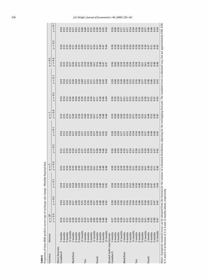
of the exchange rate change correctly. For one thing, this metricis robust to the possibility of outliers that artificially improveor degrade predictive performance. Tables 6 and 7 report theproportion of times that it predicts the correct sign of the exchangerate change in the monthly and quarterly datasets, respectively. Innearly every case, BMA predicts the correct sign more than halfthe time for the Canadian dollar, mark/euro and yen. Typically,BMA predicts the correct sign of the returns less than half the timefor the pound. For a few currency pair–horizon–hyperparametercombinations, the proportion of times that BMA predicts the signof the exchange rate change correctly is significantly greater than0.5. Cheung et al. (2002) also considered forecasting exchange ratesover the 1990s, but not using Bayesian methods. They found thatthey were able to predict the direction of exchange rate changesmore than half the time, but nonetheless typically underperformedthe randomwalk inmean square error. These results are verymuchconsistent with the idea that model and parameter uncertainty arethe stumbling blocks to exchange rate forecasting (given that theexchange rate is so close to being a random walk), and that theresearcherwhowants to get good out-of-sample prediction, ratherthan in-sample fit, should use shrinkage methods, such as BMA.

3.6. Forecasting at longer horizons

In this paper, I have reported exchange rate forecasting atshort to medium horizons, up to one year. These are the horizonsconsidered by Meese and Rogoff (1983). Some more recentauthors have found that exchange rates are more forecastable atlonger horizons, although others like Kilian (1999) have arguedconvincingly that there is no evidence of higher predictability atlonger horizons once the issues of statistical inference in long-horizon regressions are taken into account. In Tables 1 and 2,the performance of BMA relative to the random walk generallydeteriorates slightly as the horizon increases from three monthsto one year. I have also experimented with using BMA to forecastexchange rates at horizons longer than one year, but found that itsperformance relative to the randomwalk degrades further at theselonger horizons.


Table2

Out-of-sampleRMSPEforBayesianmodelaveraging—Quarterlydata

Currency

Horizon

ϕ=20

ϕ=5

ϕ=1

ϕ=0.5

ρ=0.4

ρ=0.2

ρ=0.1

ρ=0.4

ρ=0.2

ρ=0.1

ρ=0.4

ρ=0.2

ρ=0.1

ρ=0.4

ρ=0.2

ρ=0.1

Directforecasts

Canadian$

1quarter

1.040

1.014

1.001

0.975

0.967

0.973

0.951

0.968

0.979

0.976

0.986

0.991

2quarters

1.186

1.067

1.032

1.088

1.032

1.014

0.974

0.985

0.992

0.984

0.991

0.996

3quarters

1.097

1.063

1.045

1.041

1.020

1.020

0.974

0.984

0.992

0.984

0.990

0.995

4quarters

1.301

1.103

1.054

1.204

1.077

1.047

1.020

1.007

1.005

1.003

1.001

1.001

Mark/Euro

1quarter

1.043

1.053

1.064

0.990

0.989

0.995

0.965

0.964

0.969

0.980

0.981

0.985

2quarters

1.185

1.165

1.143

1.082

1.051

1.044

0.976

0.969

0.976

0.982

0.983

0.988

3quarters

1.186

1.122

1.087

1.069

1.033

1.017

0.961

0.964

0.974

0.975

0.981

0.988

4quarters

1.530

0.984

0.988

1.379

0.973

0.965

0.992

0.966

0.978

0.984

0.984

0.990

Yen

1quarter

1.102

1.085

1.083

1.029

1.019

1.019

0.974

0.977

0.981

0.984

0.987

0.990

2quarters

1.203

1.082

1.001

1.078

1.016

0.979

0.966

0.968

0.975

0.978

0.983

0.989

3quarters

2.452

1.444

1.030

1.752

1.233

1.000

0.985

0.961

0.971

0.972

0.978

0.986

4quarters

2.016

1.094

1.007

1.634

1.082

1.002

1.014

0.978

0.984

0.987

0.985

0.991

Pound

1quarter

1.311

1.205

1.113

1.209

1.147

1.085

1.040

1.020

1.009

1.013

1.005

1.003

2quarters

1.809

1.245

1.046

1.639

1.268

1.078

1.132

1.054

1.024

1.045

1.020

1.010

3quarters

2.150

1.113

1.020

1.914

1.217

1.049

1.155

1.058

1.023

1.054

1.022

1.010

4quarters

2.142

1.498

1.103

1.589

1.327

1.127

1.096

1.049

1.025

1.033

1.017

1.010


Canadian$

1quarter

1.040

1.014

1.001

0.975

0.967

0.973

0.951

0.968

0.979

0.976

0.986

0.991

2quarters

1.142

1.126

1.077

1.030

1.030

1.025

0.954

0.976

0.988

0.976

0.988

0.994

3quarters

1.163

1.133

1.050

1.024

1.018

0.999

0.932

0.961

0.976

0.965

0.982

0.990

4quarters

1.249

1.208

1.087

1.085

1.072

1.029

0.947

0.971

0.983

0.970

0.985

0.992

Mark/Euro

1quarter

1.043

1.053

1.064

0.990

0.989

0.995

0.965

0.964

0.969

0.980

0.981

0.985

2quarters

1.107

1.110

1.121

1.023

1.015

1.019

0.963

0.963

0.967

0.978

0.980

0.985

3quarters

1.163

1.157

1.168

1.049

1.034

1.036

0.956

0.958

0.964

0.973

0.977

0.983

4quarters

1.241

1.207

1.208

1.107

1.069

1.061

0.966

0.965

0.969

0.976

0.980

0.985

Yen

1quarter

1.102

1.085

1.083

1.029

1.019

1.019

0.974

0.977

0.981

0.984

0.987

0.990

2quarters

1.265

1.242

1.227

1.118

1.103

1.097

0.980

0.982

0.984

0.984

0.987

0.990

3quarters

1.404

1.398

1.371

1.161

1.159

1.150

0.954

0.960

0.965

0.967

0.974

0.981

4quarters

1.490

1.509

1.483

1.188

1.205

1.201

0.943

0.954

0.961

0.960

0.970

0.978

Pound

1quarter

1.311

1.205

1.113

1.209

1.147

1.085

1.040

1.020

1.009

1.013

1.005

1.003

2quarters

1.663

1.454

1.258

1.458

1.328

1.194

1.097

1.053

1.027

1.033

1.017

1.009

3quarters

2.145

1.845

1.516

1.778

1.586

1.365

1.158

1.087

1.042

1.052

1.026

1.013

4quarters

2.550

2.189

1.753

2.043

1.812

1.526

1.210

1.122

1.060

1.069

1.036

1.019

Notes:AsforTable1,exceptthatquarterlydataareused.


Table3

p-valuesinteststhatBMA&randomwalkhaveequalout-of-sampleRMSPE—monthlyfinancialdata

Currency

Horizon

ϕ=20

ϕ=5

ϕ=1

ϕ=0.5

ρ=0.4

ρ=0.2

ρ=0.1

ρ=0.4

ρ=0.2

ρ=0.1

ρ=0.4

ρ=0.2

ρ=0.1

ρ=0.4

ρ=0.2

ρ=0.1

Directforecasts

Canadian$

3months

0.44

0.57

0.64

0.26

0.33

0.41

0.21

0.26

0.30

0.26

0.31

0.33

6months

0.44

0.46

0.45

0.33

0.35

0.38

0.27

0.31

0.32

0.30

0.34

0.36

9months

0.87

0.77

0.64

0.69

0.61

0.50

0.28

0.27

0.28

0.29

0.31

0.32

12months

0.51

0.61

0.65

0.41

0.49

0.56

0.32

0.36

0.39

0.35

0.38

0.39

Mark/Euro

3months

0.69

0.89

0.95

0.10

0.11

0.13

0.08

0.07

0.07

0.10

0.11

0.12

6months

0.75

0.89

0.90

0.25

0.43

0.59

0.13

0.13

0.14

0.18

0.19

0.17

9months

0.79

0.88

0.90

0.45

0.63

0.75

0.24

0.25

0.26

0.27

0.28

0.28

12months

0.89

0.91

0.94

0.70

0.68

0.80

0.24

0.25

0.29

0.26

0.28

0.29

Yen

3months

0.08

0.05

0.03

0.06

0.05

0.03

0.10

0.08

0.08

0.15

0.15

0.14

6months

0.06

0.02

0.01

0.05

0.02

0.02

0.08

0.07

0.07

0.17

0.15

0.14

9months

0.19

0.08

0.07

0.17

0.11

0.08

0.17

0.16

0.16

0.22

0.20

0.20

12months

0.06

0.05

0.05

0.06

0.06

0.06

0.09

0.12

0.13

0.17

0.17

0.19

Pound

3months

0.89

0.86

0.86

0.80

0.83

0.85

0.39

0.52

0.60

0.37

0.43

0.47

6months

0.90

0.82

0.81

0.87

0.81

0.80

0.44

0.49

0.55

0.39

0.45

0.47

9months

0.41

0.46

0.48

0.46

0.47

0.47

0.37

0.46

0.48

0.39

0.44

0.46

12months

0.99

0.89

0.80

0.97

0.92

0.82

0.50

0.51

0.55

0.40

0.43

0.45


Canadian$

3months

0.27

0.32

0.69

0.11

0.11

0.11

0.04

0.07

0.09

0.04

0.09

0.11

6months

0.57

0.84

0.94

0.23

0.29

0.64

0.10

0.16

0.24

0.10

0.18

0.25

9months

0.43

0.70

0.90

0.19

0.23

0.40

0.09

0.14

0.21

0.09

0.16

0.23

12months

0.43

0.73

0.90

0.22

0.27

0.50

0.13

0.19

0.26

0.12

0.21

0.27

Mark/Euro

3months

0.73

0.89

0.96

0.12

0.10

0.06

0.03

0.02

0.01

0.02

0.02

0.00

6months

0.92

0.98

0.99

0.46

0.73

0.86

0.09

0.07

0.05

0.07

0.06

0.04

9months

0.95

0.99

1.00

0.70

0.89

0.95

0.15

0.14

0.09

0.11

0.10

0.08

12months

0.95

0.99

1.00

0.74

0.91

0.96

0.22

0.20

0.17

0.18

0.17

0.14

Yen

3months

0.02

0.01

0.00

0.02

0.01

0.00

0.01

0.01

0.00

0.01

0.01

0.00

6months

0.69

0.91

0.98

0.31

0.62

0.87

0.22

0.22

0.23

0.20

0.18

0.17

9months

0.19

0.67

0.90

0.13

0.15

0.23

0.10

0.10

0.07

0.10

0.08

0.06

12months

0.15

0.36

0.81

0.12

0.13

0.14

0.11

0.09

0.06

0.13

0.09

0.06

Pound

3months

0.98

0.99

1.00

0.89

0.98

0.99

0.31

0.36

0.37

0.22

0.23

0.18

6months

0.97

0.98

1.00

0.93

0.98

0.98

0.66

0.90

0.98

0.57

0.83

0.97

9months

0.97

0.98

0.99

0.95

0.97

0.98

0.77

0.93

0.98

0.69

0.90

0.97

12months

0.97

0.98

0.99

0.96

0.98

0.98

0.86

0.96

0.98

0.82

0.93

0.98

Notes:Thistablereportsthebootstrapp-valuesforaone-sidedtestofthehypothesisthatthedriftlessrandomwalkandBayesianModelAveragingforecastshaveequalout-of-samplemeansquarepredictionerror.Specifically

theentriesarethefractionofbootstrapsamplesinwhichtheRMSPEisbelowthesamplevalueasreportedinTable1.ThebootstrapmethodologyisdescribedinAppendixB.


Table4

RootmeansquareforecastofexchangeratechangewithBayesianmodelaveraging—Monthlyfinancialdata

Currency

Horizon

ϕ=20

ϕ=5

ϕ=1

ϕ=0.5

ρ=0.4

ρ=0.2

ρ=0.1

ρ=0.4

ρ=0.2

ρ=0.1

ρ=0.4

ρ=0.2

ρ=0.1

ρ=0.4

ρ=0.2

ρ=0.1

Directforecasts

Canadian$

3months

0.37

0.18

0.09

0.39

0.24

0.14

0.16

0.10

0.06

0.07

0.04

0.03

6months

0.69

0.34

0.17

0.73

0.46

0.27

0.30

0.20

0.12

0.13

0.09

0.05

9months

2.12

1.21

0.64

1.93

1.30

0.81

0.69

0.45

0.28

0.30

0.18

0.11

12months

1.12

0.50

0.24

1.32

0.76

0.42

0.56

0.36

0.22

0.25

0.16

0.10

Mark/Euro

3months

2.05

1.87

1.61

1.56

1.43

1.27

0.51

0.42

0.34

0.21

0.16

0.11

6months

3.32

2.75

2.14

2.62

2.30

1.92

0.88

0.71

0.53

0.37

0.27

0.18

9months

3.72

2.62

1.70

3.16

2.47

1.80

1.12

0.82

0.55

0.48

0.33

0.20

12months

7.02

4.93

3.48

5.84

4.26

3.15

1.82

1.21

0.80

0.71

0.44

0.27

Yen

3months

1.40

1.03

0.69

1.18

0.97

0.74

0.42

0.34

0.25

0.18

0.14

0.10

6months

3.16

2.41

1.64

2.56

2.17

1.68

0.87

0.70

0.51

0.37

0.28

0.19

9months

3.10

1.81

1.00

2.92

2.09

1.37

1.10

0.83

0.56

0.49

0.36

0.24

12months

4.29

2.46

1.34

4.05

2.85

1.83

1.49

1.09

0.74

0.65

0.47

0.31

Pound

3months

0.77

0.30

0.13

0.84

0.43

0.21

0.29

0.17

0.09

0.12

0.07

0.04

6months

1.83

0.68

0.30

1.94

0.96

0.47

0.63

0.34

0.18

0.25

0.14

0.07

9months

0.81

0.19

0.07

1.62

0.43

0.18

0.63

0.26

0.13

0.26

0.12

0.06

12months

5.65

2.13

0.77

4.99

2.76

1.22

1.50

0.83

0.43

0.58

0.32

0.16


Canadian$

3months

0.73

0.54

0.43

0.62

0.47

0.37

0.21

0.15

0.11

0.09

0.06

0.04

6months

1.33

0.96

0.73

1.13

0.84

0.64

0.39

0.28

0.20

0.16

0.11

0.08

9months

1.87

1.35

1.03

1.60

1.18

0.90

0.56

0.39

0.29

0.23

0.16

0.11

12months

2.37

1.72

1.32

2.03

1.49

1.15

0.71

0.50

0.37

0.30

0.20

0.14

Mark/Euro

3months

2.07

2.00

1.90

1.58

1.51

1.42

0.53

0.47

0.41

0.22

0.18

0.15

6months

3.80

3.64

3.41

2.88

2.74

2.54

0.95

0.82

0.67

0.39

0.30

0.23

9months

5.29

5.08

4.74

4.00

3.81

3.52

1.31

1.12

0.90

0.53

0.41

0.30

12months

6.59

6.32

5.89

4.97

4.73

4.37

1.62

1.38

1.10

0.65

0.50

0.36

Yen

3months

1.61

1.53

1.51

1.27

1.19

1.16

0.45

0.42

0.41

0.20

0.18

0.18

6months

2.46

2.28

2.22

1.97

1.78

1.71

0.71

0.64

0.61

0.31

0.28

0.26

9months

3.35

3.10

3.02

2.69

2.43

2.33

0.97

0.87

0.84

0.42

0.38

0.36

12months

4.25

3.97

3.89

3.41

3.10

3.00

1.23

1.11

1.07

0.54

0.49

0.47

Pound

3months

1.53

1.41

1.34

1.22

1.09

1.03

0.42

0.37

0.35

0.18

0.16

0.15

6months

2.26

1.89

1.69

1.88

1.50

1.31

0.64

0.49

0.42

0.26

0.20

0.18

9months

2.91

2.33

2.01

2.46

1.87

1.57

0.83

0.60

0.50

0.34

0.24

0.21

12months

3.50

2.72

2.31

2.99

2.21

1.81

1.01

0.70

0.57

0.41

0.28

0.24

Notes:ThistablereportstherootmeansquareforecastofexchangeratechangesfromBayesianModelAveragingusingmonthlyfinancialdata.Theexchangeratewastransformedbytakinglogsandthenmultiplyingby100,

sotheelementsinthistablecanbeinterpretedasapproximatepercentagepointforecastchanges.


Table5

RootmeansquareforecastofexchangeratechangewithBayesianmodelaveraging—Quarterlydata

Currency

Horizon

ϕ=20

ϕ=5

ϕ=1

ϕ=0.5

ρ=0.4

ρ=0.2

ρ=0.1

ρ=0.4

ρ=0.2

ρ=0.1

ρ=0.4

ρ=0.2

ρ=0.1

ρ=0.4

ρ=0.2

ρ=0.1

Directforecasts

Canadian$

1quarter

1.28

1.06

0.78

1.00

0.83

0.61

0.32

0.22

0.16

0.12

0.08

0.06

2quarters

2.06

1.12

0.69

1.74

1.02

0.67

0.52

0.31

0.21

0.20

0.12

0.08

3quarters

2.14

1.57

1.16

1.83

1.34

1.05

0.64

0.45

0.33

0.28

0.19

0.13

4quarters

2.97

1.65

1.03

2.63

1.54

1.07

0.88

0.52

0.35

0.37

0.22

0.14

Mark/Euro

1quarter

2.15

2.21

2.20

1.61

1.64

1.63

0.57

0.53

0.48

0.25

0.21

0.17

2quarters

4.60

4.44

4.02

3.47

3.32

3.05

1.18

0.99

0.78

0.50

0.38

0.26

3quarters

6.14

5.29

4.29

4.83

4.19

3.48

1.70

1.32

0.94

0.73

0.51

0.32

4quarters

8.49

3.17

1.57

7.46

3.27

1.89

2.19

1.06

0.62

0.88

0.42

0.25

Yen

1quarter

2.71

2.55

2.39

2.08

1.94

1.79

0.67

0.55

0.44

0.27

0.21

0.16

2quarters

4.80

3.57

2.28

3.68

2.80

2.03

1.08

0.79

0.60

0.44

0.32

0.24

3quarters

11.25

6.44

2.48

8.36

5.25

2.66

2.11

1.28

0.85

0.80

0.52

0.36

4quarters

10.13

3.51

1.52

7.85

3.79

2.15

2.01

1.29

0.92

0.82

0.56

0.41

Pound

1quarter

1.55

1.11

0.77

1.21

0.93

0.67

0.37

0.27

0.19

0.15

0.10

0.07

2quarters

3.55

1.56

0.39

3.03

1.60

0.60

0.86

0.42

0.23

0.33

0.17

0.09

3quarters

6.03

0.78

0.17

5.42

1.45

0.38

1.35

0.46

0.20

0.50

0.19

0.09

4quarters

7.93

4.66

1.81

5.20

3.60

2.18

1.32

1.00

0.65

0.54

0.40

0.24


Canadian$

1quarter

1.28

1.06

0.78

1.00

0.83

0.61

0.32

0.22

0.16

0.12

0.08

0.06

2quarters

2.32

1.92

1.29

1.83

1.51

1.03

0.60

0.39

0.27

0.23

0.15

0.10

3quarters

3.31

2.75

1.78

2.63

2.17

1.44

0.87

0.55

0.37

0.34

0.21

0.14

4quarters

4.26

3.57

2.26

3.41

2.82

1.83

1.13

0.71

0.46

0.44

0.27

0.18

Mark/Euro

1quarter

2.15

2.21

2.20

1.61

1.64

1.63

0.57

0.53

0.48

0.25

0.21

0.17

2quarters

4.08

4.17

4.16

3.08

3.10

3.08

1.08

1.00

0.90

0.47

0.40

0.31

3quarters

5.88

5.94

5.91

4.49

4.44

4.39

1.59

1.44

1.28

0.69

0.57

0.44

4quarters

7.60

7.53

7.49

5.91

5.66

5.56

2.12

1.84

1.62

0.92

0.73

0.56

Yen

1quarter

2.71

2.55

2.39

2.08

1.94

1.79

0.67

0.55

0.44

0.27

0.21

0.16

2quarters

5.25

4.94

4.60

4.02

3.74

3.43

1.29

1.05

0.83

0.52

0.39

0.30

3quarters

7.68

7.22

6.71

5.87

5.46

4.99

1.87

1.52

1.19

0.75

0.57

0.44

4quarters

9.91

9.33

8.68

7.56

7.04

6.44

2.41

1.96

1.54

0.97

0.73

0.56

Pound

1quarter

1.55

1.11

0.77

1.21

0.93

0.67

0.37

0.27

0.19

0.15

0.10

0.07

2quarters

3.28

2.50

1.80

2.54

2.00

1.45

0.76

0.50

0.33

0.29

0.18

0.12

3quarters

5.39

4.40

3.34

4.16

3.42

2.56

1.23

0.77

0.47

0.45

0.26

0.16

4quarters

7.27

6.03

4.52

5.59

4.63

3.42

1.63

1.00

0.58

0.58

0.32

0.20

Notes:AsforTable4,exceptthatquarterlydataareused.


Table6

ProportionoftimesBMApredictscorrectsignofexchangeratechange—Monthlyfinancialdata

Currency

Horizon

ϕ=20

ϕ=5

ϕ=1

ϕ=0.5

ρ=0.4

ρ=0.2

ρ=0.1

ρ=0.4

ρ=0.2

ρ=0.1

ρ=0.4

ρ=0.2

ρ=0.1

ρ=0.4

ρ=0.2

ρ=0.1

Directforecasts

Canadian$

3months

0.54

0.54

0.54

0.53

0.53

0.54

0.53

0.54

0.54

0.53

0.54

0.54

6months

0.53

0.53

0.53

0.53

0.53

0.53

0.55

0.54

0.54

0.55

0.55

0.55

9months

0.53

0.54

0.55

0.54

0.54

0.55

0.54

0.53

0.55

0.54

0.55

0.54

12months

0.56

0.56

0.56

0.58

0.56

0.56

0.57

0.56

0.55

0.57

0.56

0.55

Mark/Euro

3months

0.58

0.57

0.54

0.59

0.59

0.57

0.58

0.58

0.58

0.56

0.57

0.57

6months

0.59

0.60

0.60

0.60

0.61

0.62

0.63

0.64

0.64

0.63

0.64

0.63

9months

0.59

0.59

0.59

0.58

0.59

0.59

0.56

0.58

0.56

0.57

0.55

0.53

12months

0.53

0.55

0.56

0.53

0.57

0.57

0.54

0.58

0.60

0.54

0.60

0.60

Yen

3months

0.59

0.54

0.52

0.60

0.53

0.52

0.60

0.54

0.51

0.59

0.52

0.48

6months

0.57

0.56

0.55

0.58

0.56

0.55

0.58

0.56

0.55

0.58

0.55

0.52

9months

0.60

0.59

0.59

0.63

0.59

0.59

0.62

0.58

0.57

0.60

0.57

0.55

12months

0.60

0.57

0.58

0.61

0.57

0.57

0.61

0.57

0.57

0.61

0.56

0.58

Pound

3months

0.50

0.49

0.49

0.52

0.49

0.49

0.51

0.51

0.50

0.52

0.51

0.49

6months

0.48

0.48

0.48

0.48

0.48

0.47

0.48

0.49

0.49

0.48

0.49

0.50

9months

0.48

0.46

0.45

0.48

0.46

0.45

0.48

0.46

0.45

0.47

0.47

0.45

12months

0.46

0.45

0.45

0.48

0.45

0.45

0.46

0.44

0.44

0.47

0.44

0.44


Canadian$

3months

0.57

0.58

0.58

0.58

0.58

0.58

0.59

0.58

0.58

0.58

0.58

0.56

6months

0.59

0.60

0.59

0.59

0.60

0.59

0.60

0.59

0.60

0.60

0.59

0.60

9months

0.59

0.59

0.58

0.59

0.59

0.58

0.60

0.59

0.58

0.60

0.58

0.58

12months

0.58

0.58

0.58

0.58

0.58

0.57

0.60

0.57

0.58

0.59

0.57

0.57

Mark/Euro

3months

0.57

0.55

0.55

0.59

0.56

0.57

0.59

0.61

0.60

0.59

0.60

0.57

6months

0.57

0.56

0.54

0.58

0.57

0.55

0.56

0.57

0.58

0.58

0.59

0.57

9months

0.54

0.54

0.52

0.56

0.54

0.54

0.55

0.55

0.55

0.56

0.56

0.54

12months

0.50

0.50

0.49

0.51

0.51

0.50

0.51

0.53

0.55

0.54

0.56

0.56

Yen

3months

0.58

0.56

0.56

0.58

0.58

0.56

0.58

0.58

0.56

0.58

0.58

0.56

6months

0.52

0.48

0.48

0.55

0.51

0.48

0.55

0.51

0.48

0.54

0.50

0.48

9months

0.62

0.59

0.59

0.62

0.59

0.58

0.62

0.59

0.57

0.61

0.58

0.56

12months

0.61

0.58

0.58

0.61

0.59

0.57

0.61

0.58

0.56

0.61

0.58

0.57

Pound

3months

0.48

0.49

0.48

0.48

0.49

0.48

0.48

0.47

0.48

0.48

0.47

0.46

6months

0.52

0.53

0.47

0.52

0.53

0.49

0.52

0.52

0.46

0.52

0.51

0.48

9months

0.49

0.47

0.45

0.51

0.47

0.46

0.49

0.47

0.43

0.48

0.45

0.43

12months

0.47

0.45

0.44

0.46

0.45

0.45

0.45

0.45

0.43

0.46

0.45

0.44

Notes:Asymptoticstandarderrorscanbeobtainedfromtheformulaforthevarianceofabinomialdistribution,adjustingfortheoverlappingforecasts.Thestandarderrorssoobtainedvary,butareapproximately0.06,0.09,

0.11and0.13athorizonsof3,6,9and12monthsahead,respectively.


Table7

ProportionoftimesBayesianmodelaveragingpredictscorrectsignofexchangeratechange—Quarterlydata

Currency

Horizon

ϕ=20

ϕ=5

ϕ=1

ϕ=0.5

ρ=0.4

ρ=0.2

ρ=0.1

ρ=0.4

ρ=0.2

ρ=0.1

ρ=0.4

ρ=0.2

ρ=0.1

ρ=0.4

ρ=0.2

ρ=0.1

Directforecasts

Canadian$

1quarter

0.63

0.63

0.64

0.64

0.61

0.59

0.64

0.63

0.59

0.63

0.64

0.63

2quarters

0.58

0.64

0.63

0.63

0.63

0.63

0.64

0.64

0.64

0.64

0.66

0.63

3quarters

0.67

0.61

0.64

0.66

0.64

0.63

0.67

0.64

0.64

0.66

0.64

0.64

4quarters

0.58

0.56

0.59

0.59

0.56

0.59

0.59

0.58

0.59

0.61

0.61

0.58

Mark/Euro

1quarter

0.55

0.55

0.55

0.55

0.55

0.55

0.56

0.55

0.56

0.58

0.55

0.58

2quarters

0.56

0.56

0.56

0.53

0.56

0.56

0.56

0.56

0.58

0.58

0.59

0.59

3quarters

0.56

0.58

0.64

0.55

0.58

0.64

0.56

0.61

0.64

0.56

0.63

0.64

4quarters

0.52

0.55

0.55

0.48

0.55

0.56

0.52

0.53

0.59

0.52

0.53

0.56

Yen

1quarter

0.64

0.64

0.64

0.64

0.64

0.64

0.63

0.64

0.59

0.63

0.59

0.58

2quarters

0.61

0.61

0.58

0.63

0.61

0.59

0.61

0.59

0.58

0.61

0.59

0.58

3quarters

0.67

0.59

0.59

0.67

0.59

0.59

0.63

0.59

0.61

0.61

0.59

0.55

4quarters

0.58

0.53

0.55

0.59

0.55

0.55

0.59

0.58

0.55

0.59

0.56

0.55

Pound

1quarter

0.53

0.56

0.59

0.53

0.56

0.58

0.55

0.59

0.61

0.58

0.58

0.56

2quarters

0.39

0.44

0.45

0.38

0.42

0.45

0.41

0.45

0.45

0.41

0.45

0.45

3quarters

0.45

0.41

0.42

0.45

0.44

0.42

0.41

0.45

0.42

0.42

0.45

0.44

4quarters

0.42

0.44

0.47

0.39

0.45

0.47

0.42

0.48

0.50

0.44

0.50

0.50


Canadian$

1quarter

0.63

0.63

0.64

0.64

0.61

0.59

0.64

0.63

0.59

0.63

0.64

0.63

2quarters

0.61

0.61

0.59

0.59

0.59

0.63

0.61

0.64

0.63

0.66

0.64

0.63

3quarters

0.69

0.67

0.64

0.69

0.67

0.66

0.69

0.69

0.67

0.69

0.69

0.67

4quarters

0.67

0.66

0.61

0.67

0.67

0.64

0.67

0.67

0.64

0.67

0.67

0.66

Mark/Euro

1quarter

0.55

0.55

0.55

0.55

0.55

0.55

0.56

0.55

0.56

0.58

0.55

0.58

2quarters

0.55

0.58

0.58

0.55

0.56

0.55

0.56

0.56

0.59

0.59

0.59

0.58

3quarters

0.50

0.50

0.48

0.52

0.53

0.48

0.55

0.52

0.53

0.55

0.55

0.55

4quarters

0.50

0.48

0.47

0.50

0.53

0.47

0.56

0.52

0.55

0.58

0.55

0.56

Yen

1quarter

0.64

0.64

0.64

0.64

0.64

0.64

0.63

0.64

0.59

0.63

0.59

0.58

2quarters

0.59

0.59

0.59

0.59

0.59

0.59

0.59

0.59

0.59

0.59

0.59

0.58

3quarters

0.69

0.66

0.66

0.69

0.66

0.66

0.69

0.69

0.69

0.69

0.70

0.67

4quarters

0.69

0.66

0.64

0.69

0.66

0.64

0.69

0.67

0.69

0.69

0.72

0.67

Pound

1quarter

0.53

0.56

0.59

0.53

0.56

0.58

0.55

0.59

0.61

0.58

0.58

0.56

2quarters

0.44

0.48

0.55

0.42

0.42

0.55

0.42

0.53

0.55

0.45

0.55

0.56

3quarters

0.41

0.41

0.52

0.41

0.39

0.52

0.41

0.47

0.52

0.42

0.47

0.52

4quarters

0.38

0.38

0.47

0.38

0.36

0.47

0.38

0.42

0.45

0.38

0.42

0.42

Notes:Asymptoticstandarderrorscanbeobtainedfromtheformulaforthevarianceofabinomialdistribution,adjustingfortheoverlappingforecasts.Thestandarderrorssoobtainedvary,butareapproximately0.06,0.09,

0.11and0.13athorizonsof1,2,3and4quartersahead,respectively.


Table 8Out-of-sample RMSPE for equal-weighted averaged forecasts

Horizon Canadian $ Mark/Euro Yen Pound

Direct forecasts—monthly financial data3 months 1.010 0.969 0.994 1.0246 months 1.030 0.960 1.006 1.0539 months 1.055 0.975 1.012 1.07712 months 1.075 0.983 1.036 1.097

Direct forecasts—quarterly data

1 quarter 0.989 0.969 0.999 1.0262 quarter 1.014 0.975 1.016 1.0683 quarter 1.034 0.986 1.032 1.0924 quarter 1.068 0.998 1.081 1.111

Iterated multi-step forecasts—monthly financial data

3 months 1.006 0.970 0.992 1.0216 months 1.021 0.973 1.020 1.0519 months 1.029 0.973 1.017 1.08212 months 1.042 0.983 1.033 1.113

Iterated multi-step forecasts—quarterly data

1 quarter 0.989 0.969 0.999 1.0262 quarter 1.009 0.980 1.024 1.0653 quarter 1.015 0.984 1.032 1.0974 quarter 1.035 0.999 1.064 1.128

Notes: This table reports the out-of-sample relative mean square prediction errorfrom the forecasts taken by simple equal-weighted averaging of different modelforecasts, relative to themean square prediction error from a driftless randomwalkforecast. Themodels each have a constant and just one other predictor, as describedin the text.

3.7. Comparison with equal weighted model averaging

The efficacy of BMA is conceptually related to the idea thatis very much part of the folklore of the forecasting literaturethat taking forecasts from several different models and simplyaveraging them gives better predictions than any one model on itsown (Bates and Granger, 1969; Stock and Watson, 2001, 2004).I therefore experimented with taking all regression models of

the form of Eq. (6) with a single right hand side predictor, plusa constant, using all the predictors that I have in the monthlyand quarterly datasets, augmented with the monthly long-terminterest rate and the quarterly monetary fundamentals of Mark(1995). These last two predictors could not be included in theBMAexercise using all possible permutations of regressors becausethis would have generated a problem of perfect multicollinearity.This gives a total of 8 models in the monthly dataset and17 in the quarterly dataset. Needless to say, no one of thesemodels gives consistently good forecasting performance. The out-of-sample relative mean square prediction error obtained fromsimply averaging all of these forecasts, relative to the driftlessrandom walk benchmark, is reported in Table 8. Results from thesame exercise using Eqs. (9) and (10) are also reported. A numbergreater than 1 means that equal-weighted model-averaging isforecasting lesswell than a randomwalk. Except for themark/euro,most entries in the tables are greater than 1. Simple equal-weighted model averaging, that is such an effective strategy inmany forecasting contexts, does not seem to buy us so much inexchange rate forecasting, at least not with these models.

4. Conclusion

In this paper I have considered a specific approach to poolingthe forecasts from different models, namely Bayesian ModelAveraging, and argued that it gives promising results for out-of-sample exchange rate prediction. Formost currency–horizon pairs,with a sufficiently high degree of shrinkage, the Bayesian ModelAveraging forecasts yield mean square prediction errors modestlylower than one obtains from a random walk forecast. Though

the improvements are modest, this nonetheless stands in markedcontrast to the results obtained in the exchange rate forecastingliterature at horizons of one year or less without using shrinkagemethods. The forecasts generated by Bayesianmodel averaging arevery close to those from a random walk forecast.The sole focus in this paper has been on establishing whether

Bayesian Model Averaging methods seem to work in the senseof beating random walk forecasts out-of-sample. One does nothave to believe that the model and parameter priors used in thispaper are genuine subjective prior beliefs to view Bayesian ModelAveraging as practically useful. Moreover, viewing BayesianModelAveraging as practically useful does not rule out the possibility thatother related shrinkage techniques are useful too.In future work, it would be possible and interesting to

includenonlinearmodels, notablyMarkov switching and thresholdmodels in the model averaging exercise. Such models have beenconsidered by Engel and Hamilton (1990), Meese and Rose (1991)and Kilian and Taylor (2003) among others. These models maycontain information that could make them useful as elements ofa forecast pooling exercise such as Bayesian Model Averaging.

Acknowledgment

I am grateful to Ben Bernanke, David Bowman, Jon Faust, MattPritsker and Pietro Veronesi for helpful comments, and to SergeyChernenko for excellent research assistance. The views in thispaper are solely the responsibility of the author.

Appendix A. Data sources

Exchange Rates:Monthly average of daily rates, Federal ReserveH-10 Release.Long Term Interest Rates: 10 year rates from MEI and IMF

International Financial Statistics (IFS).Short Term Interest Rates: 3-month rates, except call money

rate for Japan, all from MEI.Prices∗: CPI from MEI. Seasonally adjusted.GDP∗: MEI (real, sa).LaborProductivity∗: GDP (real, sa) divided by total civilian

employment (sa), both from MEI.MoneyStock∗: M1 from MEI (sa) except M4 for the United

Kingdom.Monetaryfundamentals∗: Computed from money stock, GDP

and prices.Stock Prices: Morgan Stanley Capital International (MSCI) price

indices (local currency).Dividend Yields: MSCI.CurrentAccount∗: MEI (sa).CurrentAccount/GDPratio∗: Current Account (sa) divided by

GDP (nominal, sa). both from MEI.∗: included in quarterly dataset only.

Appendix B. Construction of bootstrap samples

To construct bootstrap samples in the monthly dataset, I fitteda VAR(12) to the exchange rate, log relative stock prices, therelative dividend yield, relative short term interest rates, therelative term spread. I estimated this 5-variable VAR but anchoredthe bootstrap at the bias-adjusted estimates of Kilian (1998),not the OLS estimates. I also imposed that all the coefficients inthe exchange rate equation were equal to zero, except for thecoefficient on the first lag of the exchange ratewhich I set to one. Sothe exchange rate is a driftless random walk by construction (thenull hypothesis of no forecastability is imposed). I then generated500 bootstrap samples of all of the variables in this VAR. All of thepredictors in the monthly dataset can be constructed from these 6


variables. So in this way I get a bootstrap sample of the exchangerate and all of the predictors inwhich the exchange rate is a randomwalk (but may affect future values of the predictors and so is notstrictly exogenous).

References

Avramov, D., 2002. Stock return predictability and model uncertainty. Journal ofFinancial Economics 64, 423–458.

Bates, J.M., Granger, C.W.J., 1969. The combination of forecasts. Operations ResearchQuarterly 20, 451–468.

Bekaert, G., Hodrick, R.J., 1992. Characterizing predictable components in excessreturns on equity and foreign exchange markets. Journal of Finance 47,467–509.

Bernanke, B.S., Boivin, J., 2003. Monetary policy in a data-rich environment. Journalof Monetary Economics 50, 525–546.

Cheung, Y-W, Chinn, M.D., Pascual, A.G., 2002. Empirical exchange rate models ofthe nineties: Are any fit to survive? NBER Working Paper 9393.

Chipman, H., George, E.I., McCulloch, R.E., 2001. The practical implementation ofBayesian model selection, mimeo.

Clarida, R.H., 2003. The out-of-sample success of term structure models: A stepbeyond. Journal of International Economics 60, 61–83.

Cremers, K.J.M., 2002. Stock return predictability: A Bayesian model selectionperspective. Review of Financial Studies 15, 1223–1249.

Doppelhofer, G., Miller, R.I., Sala-i-Martin, X., 2000. Determinants of long-termgrowth: A Bayesian averaging of classical estimates (BACE) approach. NBERWorking Paper 7750.

Dornbusch, R., 1976. Expectations and exchange rate dynamics. Journal of PoliticalEconomy 84, 1161–1171.

Engel, C., Hamilton, J.D., 1990. Long swings in the dollar: Are they in the data anddo markets know it? American Economic Review 80, 689–713.

Faust, J., Rogers, J.H., Wright, J.H., 2003. Exchange rate forecasting: The errors we’vereally made. Journal of International Economics 60, 35–59.

Fernandez, C., Ley, E., Steel, M.F.J., 2001. Model uncertainty in cross-country growthregressions. Journal of Applied Econometrics 16, 563–576.

Fernández-Villaverde, J., Rubio-Ramírez, J.F., 2004. Comparing dynamic equilibriummodels to data: A Bayesian approach. Journal of Econometrics 123, 153–187.

Groen, J.J., 1999. Long horizon predictability of exchange rates: Is it for real?Empirical Economics 24, 451–469.

Hjort, N.L., Claeskens, G., 2003. Frequentist model average estimators. Journal of theAmerican Statistical Association 98, 879–899.

Hoeting, J.A., Madigan, D., Raftery, A.E., Volinsky, C.T., 1999. Bayesian modelaveraging: A tutorial. Statistical Science 14, 382–417.

Kass, R.E., Raftery, A.E., 1995. Bayes factors. Journal of the American StatisticalAssociation 90, 773–795.

Key, J.T., Pericchi, L.R., Smith, A.F.M., 1998. Choosing among models when none ofthem are true. In: Racugno, W. (Ed.), Proceedings of the Workshop on ModelSelection, Special Issue of Rassegna diMetodi Statistici ed Applicazioni. PitagoreEditrice, Bologna.

Kilian, L., 1998. Small-sample confidence intervals for impulse response functions.Review of Economics and Statistics 80, 218–230.

Kilian, L., 1999. Exchange rates andmonetary fundamentals:What dowe learn fromlong-horizon regressions? Journal of Applied Econometrics 14, 491–510.

Kilian, L., Taylor, M.P., 2003. Why is it so difficult to beat the random walk forecastof exchange rates? Journal of International Economics 60, 85–107.

Koop, G., Potter, S., 2003. Forecasting in largemacroeconomic panels using Bayesianmodel averaging. Federal Reserve Bank of New York Staff Report 163.

Leamer, E.E., 1978. Specification Searches. Wiley, New York.Marcellino, M., Stock, J.H., Watson, M.W., 2006. A comparison of direct and iteratedmultistep AR methods for forecasting macroeconomic time series. Journal ofEconometrics 135, 499–526.

Mark, N., 1995. Exchange rates and fundamentals: Evidence on long-horizonpredictability. American Economic Review 85, 201–218.

Meese, R., Rose, A.K., 1991. An empirical assessment of nonlinearities in models ofexchange rate determination. Review of Economic Studies 58, 603–619.

Meese, R., Rogoff, K., 1983. Empirical exchange ratemodels of the seventies: Do theyfit out of sample? Journal of International Economics 14, 3–24.

Min, C., Zellner, A., 1993. Bayesian and non-Bayesian methods for combiningmodels and forecasts with applications to forecasting international growthrates. Journal of Econometrics 56, 89–118.

Raftery, A.E., Madigan, D., Hoeting, J.A., 1997. Bayesian model averaging for linearregression models. Journal of the American Statistical Association 92, 179–191.

Stock, J.H., Watson, M.W., 2001. Forecasting output and inflation: The role of assetprices, mimeo.

Stock, J.H., Watson, M.W., 2002. Forecasting using principal components from alarge number of predictors. Journal of the American Statistical Association 97,1167–1179.

Stock, J.H., Watson, M.W., 2004. Combination forecasts of output growth in a sevencountry dataset. Journal of Forecasting 23, 405–430.

Stock, J.H.,Watson,M.W., 2005. An empirical comparison ofmethods for forecastingusing many predictors, mimeo.

Zellner, A., 1971. An Introduction to Bayesian Inference in Econometrics. Wiley,New York.

bayesian model averaging and exchange rate forecasts

Documents