'

&

$

%

Basics of Probability Theory and Random

Processes

Basics of probability theory a

• Probability of an event E represented by P (E) and is given by

P (E) =NE

NS

(1)

where, NS is the number of times the experiment is performed

and NE is number of times the event E occured.

Equation 1 is only an approximation. For this to represent the

exact probability NS → ∞.

The above estimate is therefore referred to as Relative

Probability

Clearly, 0 ≤ P (E) ≤ 1.arequired for understanding communication systems

'

&

$

%

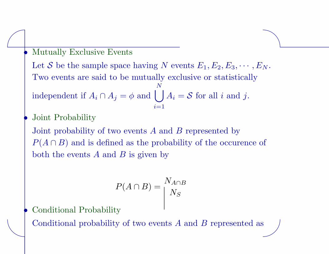
• Mutually Exclusive Events

Let S be the sample space having N events E1, E2, E3, · · · , EN .

Two events are said to be mutually exclusive or statistically

independent if Ai ∩ Aj = φ andN⋃

i=1

Ai = S for all i and j.

• Joint Probability

Joint probability of two events A and B represented by

P (A ∩ B) and is defined as the probability of the occurence of

both the events A and B is given by

P (A ∩ B) =NA∩B

NS

• Conditional Probability

Conditional probability of two events A and B represented as

'

&

$

%

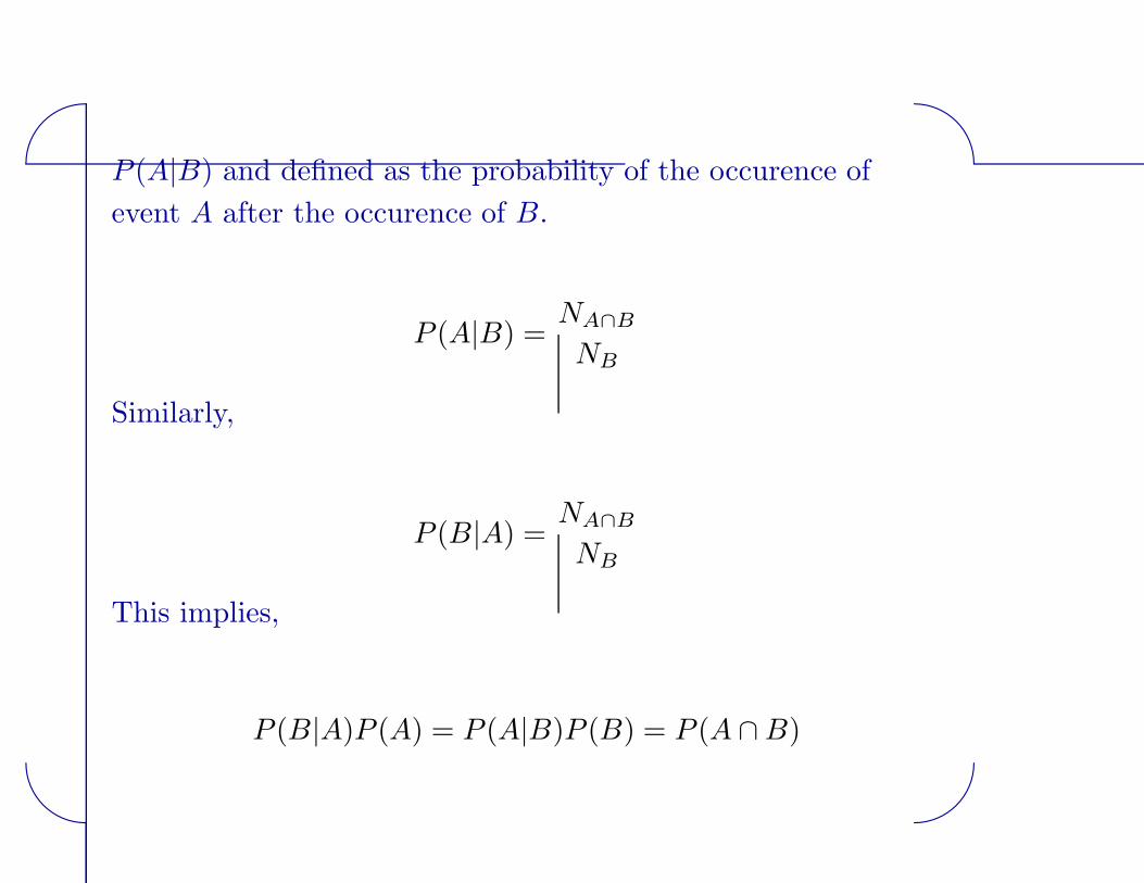
P (A|B) and defined as the probability of the occurence of

event A after the occurence of B.

P (A|B) =NA∩B

NB

Similarly,

P (B|A) =NA∩B

NB

This implies,

P (B|A)P (A) = P (A|B)P (B) = P (A ∩ B)

'

&

$

%

• Chain Rule

Let us consider a chain of events A1, A2, A3, · · · , AN which are

dependent on each other. Then the probability of occurence of

the sequence

P (AN , AN−1, AN−2,

· · · , A2, A1)

= P (AN |AN−1, AN−2, · · · , A1).

P (AN−1|AN−2, AN−3, · · · , A1).

· · · .P (A2|A1).P (A1)

'

&

$

%

Bayes Rule

AA

A

A

A

B2

1

34

5

Figure 1: The partition space

In the above figure, if A1, A2, A3, A4, A5 partition the sample space

S, then (A1 ∩ B), (A2 ∩ B), (A3 ∩ B), (A4 ∩ B), and (A5 ∩ B)

partition B.

Therefore,

'

&

$

%

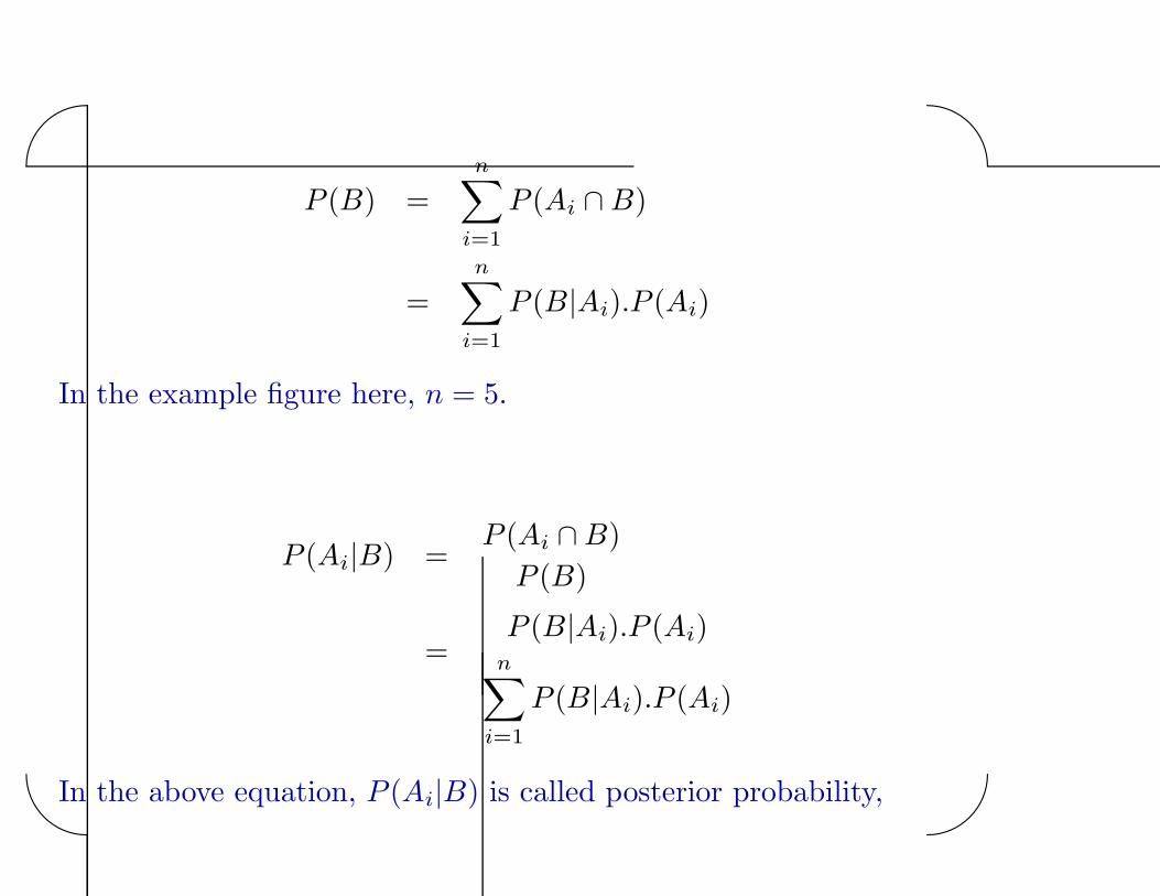
P (B) =n∑

i=1

P (Ai ∩ B)

=n∑

i=1

P (B|Ai).P (Ai)

In the example figure here, n = 5.

P (Ai|B) =P (Ai ∩ B)

P (B)

=P (B|Ai).P (Ai)

n∑i=1

P (B|Ai).P (Ai)

In the above equation, P (Ai|B) is called posterior probability,

'

&

$

%

P (B|Ai) is called likelihood, P (Ai) is called prior probability andn∑

i=1

P (B|Ai).P (Ai) is called evidence.

'

&

$

%

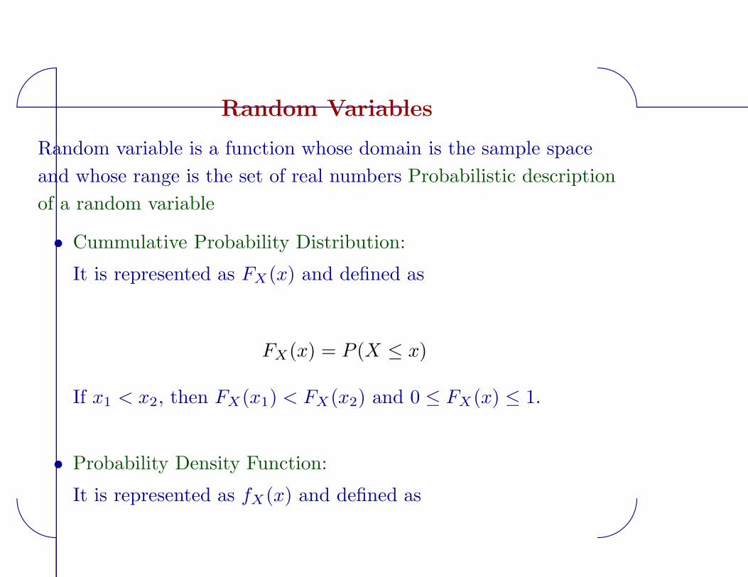
Random Variables

Random variable is a function whose domain is the sample space

and whose range is the set of real numbers Probabilistic description

of a random variable

• Cummulative Probability Distribution:

It is represented as FX(x) and defined as

FX(x) = P (X ≤ x)

If x1 < x2, then FX(x1) < FX(x2) and 0 ≤ FX(x) ≤ 1.

• Probability Density Function:

It is represented as fX(x) and defined as

'

&

$

%

fX(x) =dFX(x)

dx

This implies,

P (x1 ≤ X ≤ x2) =

∫ x2

x1

fX(x) dx

fX(x) =dFX(x)

dx