Basics of color based computer vision implemented inMatlabLuijten, H.J.C.

Published: 01/01/2005

Document VersionPublisher’s PDF, also known as Version of Record (includes final page, issue and volume numbers)

Please check the document version of this publication:

• A submitted manuscript is the author's version of the article upon submission and before peer-review. There can be important differencesbetween the submitted version and the official published version of record. People interested in the research are advised to contact theauthor for the final version of the publication, or visit the DOI to the publisher's website.• The final author version and the galley proof are versions of the publication after peer review.• The final published version features the final layout of the paper including the volume, issue and page numbers.

Link to publication

General rightsCopyright and moral rights for the publications made accessible in the public portal are retained by the authors and/or other copyright ownersand it is a condition of accessing publications that users recognise and abide by the legal requirements associated with these rights.

• Users may download and print one copy of any publication from the public portal for the purpose of private study or research. • You may not further distribute the material or use it for any profit-making activity or commercial gain • You may freely distribute the URL identifying the publication in the public portal ?

Take down policyIf you believe that this document breaches copyright please contact us providing details, and we will remove access to the work immediatelyand investigate your claim.

Download date: 15. Jul. 2018

Basics of color based computervision implemented in Matlab

H.J.C. Luijten

DCT 2005.87

Traineeship report

Coach(es): dr.ir. M.J.G. van de Molengraft

Supervisor: prof.dr.ir. M. Steinbuch

Technische Universiteit EindhovenDepartment Mechanical EngineeringDynamics and Control Technology Group

Eindhoven, June, 2005

Index 1. Introduction 1 2. Vision through the years 2

2.1 Laser 2 2.2 Sonar 2 2.3 Camera vision 2 2.4 Omni directional view 3 2.5 Future 3

3. Camera vision in a Robocup environment 4 4. Color recognition 5

4.1 Color space 5 4.1.1 RGB-space 5 4.1.2 HSV-space 6 4.1.3 LAB-space 6

4.2 Color definition 7 4.2.1 HSV-space 7 4.2.2 RGB- / LAB-space 7 4.2.3 Color definition using Matlab 7

4.3 Pixel labeling 9 4.3.1 Pixel labeling using Matlab 9 4.3.2 Speed of pixel labeling 10

5. Object localization 11 5.1 Noise 11 5.2 Method 1: Mean and standard deviation 12 5.3 Method 2: variance 13 5.4 Object localization in front of the robot 14

5.4.1 XY / RD relation 15 6. Vision implementation in Matlab/Simulink 16

6.1 Matlab 16 6.1.1 Results 16

6.2 Simulink 17 7. Conclusion 19 8. References 20 Appendix A: Explanation of Matlab functions 21 Appendix B: Matlab code for color definition 22 Appendix C: Matlab code for pixel labeling 23 Appendix D: Matlab code for object recognition 24

1. Introduction It has always been a dream to have a robot with the same abilities as a human being. Ten years ago, people could only imagine the things robots are capable of today, but the road to an autonomous robot that can act as a human, is still very long. To improve the abilities of robots to act like real humans, a group of people decided to form an organization to stimulate the progress in robotics and artificial intelligence. They thought of a way to get many people interested in the subject and they came up with the idea of robots playing soccer. The robocup organization was born and its goal is very clear: By the year 2050, develop a team of fully autonomous humanoid robots that can win against the human world champion team in soccer. The fact that these robots have to be autonomous means that they have to do everything without interference of humans. One of the keys to success is a good vision system, so the question is: how to make a robot see like a human? The only way for now to approach human sight is with the use of a camera, so that is what will be further developed in the future. This report will take the Robocup middle size league as an example to apply a vision system to. The goal is to make a fast program for ball localization with Matlab that can capture images from a video device and calculate the position of the ball in front of the robot. The report will begin with an analysis of different ways to implement vision on a robot through the years. After this the basic steps of camera vision and its theory are discussed and implemented in Matlab. At the end the implementation of the entire system in Matlab is discussed and the final results are shown.

1

2. Vision systems through the years With the start of the Robocup project, the quest for a suitable method to implement vision began. The main targets of a vision system are self-localization and object recognition. Because of the fact that the technology is getting better and better every year, the rules of robocup matches change every year. The goal is to make robots just like humans, so the rules of the game are getting more realistic and the restrictions on the robots too. A couple of years ago computers were by far not as fast as today. Camera vision was not the first option, so the participants of the Robocup leagues thought of other ways to implement vision on their robots.

2.1 Laser A very important thing for the robot to know is if an object is near the robot, so when he is moving he can avoid it. This information is easy to obtain by using infrared lasers and sensors. The principle is very simple. The laser sends out an infrared beam which will be reflected to the sensor. The time between the emission and the reflection on the sensor is a measure for the distance between the object and the robot. [1] The laser is usually attached near the bottom of the robot to make sure the beam won’t go over the ball. This system is very reliable when it comes to object localization, but it is not sufficient for a complete robot vision system.

2.2 Sonar Another method with the same purpose as the infrared laser is sonar. The principle is the same as the infrared laser, only in this case a sound wave with a high frequency is sent out, which will be reflected. The time between emission and reflection is again a measure for the distance. [2] This system is, just as the infrared laser, very reliable and can serve as an extra option for the robots, but it’s not sufficient as a complete vision system.

2.3 Camera vision With one of these systems on board, the robot must be able to avoid crashes with other robots, but the main targets are not accomplished. The only thing that is known, is the distance between the robot and the nearest object in every direction. With a simple form of camera vision, an important task can be fulfilled, namely the recognition of the ball. The implementation of a simple camera, connected to a computer, on top of the robot and some software are the solution. The camera sends images to a software program that can recognize the color of the ball. With this information the place off the ball in the image is known and thus the angle between the ball and the front of the robot can be measured. [3] Together with the information of the infrared sensor or the sonar system, the software can calculate where the ball is in relation to the robot. Self localization was pretty difficult with this system, so most

2

of the time the robots used the position at the start of the match and the track it followed to calculate the present position.

2.4 Omni directional view Because of the relative small angle that a normal camera can cover, a new system was developed. This system uses a conical mirror and a camera. The principle is very simple. Point the camera to the air and place the mirror right above the camera (figure 1.1). With this system, the robot can see all around him because of the conical shape of the camera. The images are analyzed with the same color recognition software and with a little more effort the position of objects can be calculated. [4] Self localization is also possible with this system, because of the typical poles at each corner of the field. With the omni directional view there are almost all the time 2 poles in sight. With the distance to those poles and the angle between the poles and the robot, the location of the robot in the field can be calculated.

Figure 2.1: Schematic view of an omnivision device

2.5 Future vision systems Although Omni directional vision is very useful in the Robocup middle league, it is not a very realistic way of implementing vision. Therefore it might be prohibited within a couple of years [5]. With the development of computers, also the performances of camera vision increased. Computers are getting faster every day, and so are the algorithms for image segmentation and object localization. Therefore the future of robot vision is dependent on the development of computers. The frequency with which images can be processed grows along with the speed of computers, and with the proper software for object recognition, computer vision can become very successful.

3

3. Camera vision in a Robocup environment In the previous chapter camera vision is described as simple as a camera connected with a computer with a little bit of software. The reality shows us that it is not as easy as it sounds. A computer can use colors for object recognition. To be able to recognize colors, these colors have to be defined. Because in real life, an object rarely has a homogenous color, it is very difficult to recognize objects. In a Robocup environment, object recognition is made easier. Every important object in the field has its own, almost homogenous, color. The important objects and their colors are shown in table 3.1. [5]

Object Color Ball Red/orange Goal1 / Goal2 Yellow / Blue Robots Black Field Green Lines White Cornerpost Yellow/blue stripes

Table 3.1: Colors in a robocup field.

The main target in this report is the ball. As can be seen in table 3.1, the color of the ball is red/orange. This means that in every robocupmatch the ball has almost the same red/orange color and other objects in the field may not have this color. It can always occur that another object with the same color is next to the field and therefore in sight of the camera. This can disturb the functioning of the vision system, but a solution for this problem is found. Vision in a robocup environment is thus not completely realistic, because of the restricted colors of important objects. Until computers are fast enough and new algorithms are developed, this restriction is necessary to be able to recognize the important objects.

4

4. Color recognition To understand the basics of camera vision it is necessary to know how a computer sees an image. A computer can only work with numbers, so when an image is imported on a computer, the computer sees it as a lot of numbers. For each pixel in the image, the computer uses a code and all those codes together form the total image. For image processing, it is required to understand the way a computer encodes an image. There is more than one way to encode a picture by using different color spaces. In this chapter different color spaces are described. Once these codes are analyzed, they can be used for color definition and when the colors are defined, pixel labeling is used to recognize colors in the picture. [6]

4.1 Color space A color space describes the range of colors that a camera can see. It is a collection of codes for every color. Each pixel in an image has a color that is described in the color space, so this color space can be used for pixel labeling. There are different ways to describe all colors, so there are also different color spaces. In this section 3 of most well known color spaces are described. The size of a color space depends on the number of tones of a main color. [7]

4.1.1 RGB-space In the RGB color space, each color is described as a combination of three main colors, namely Red, Green and Blue. This color space can be visualized as a 3d matrix with the main colors set out on the axis (figure 4.1). The values for the main colors vary from 0 to 1.

Figure 4.1: RGB color spacemodel.

Each color is coded with three values, a value for red, blue and green. In this color space, an imported image on a computer is thus transformed into 3 matrices with values per pixel for the representing main color.

5

4.1.2 HSV-space Another color space is the HSV space. This is a cylindrical space and can be modeled as a cone turned upside down (figure 4.2). The vertical position defines the brightness (V), the angular position defines the hue (H) and the radial position represents the saturation (S). For every value of V, a circle can be drawn as a cross section of the cone (figure 4.3). The saturation always ranges from 0 to 1 and it specifies the relative position from the vertical axis to the side of the circle. Zero saturation indicates no hue, just gray scale. The hue is what is normally thought of as color and varies from 0 to 1. Brightness ranges also from 0 to 1, where V=0 indicates black.

Just like in the RGB space, a color in this space is also coded with 3 values. Therefore an image is also transformed into three matrices when imported on a computer.

4.1.3 LAB-space The last color space that will be discussed is the LAB space. This is also a color space with three parameters. L defines lightness, A denotes the red/green value and B the yellow/blue value. This color space is not as easy to visualize as the other two spaces, because L is a value between 0 and 100 and for every value of L, another picture with a specific color range can be drawn. In these pictures the A value is on the horizontal and B the vertical axis. In figure 4.4 an example can be seen for an L-value of 77.

Figure 4.2: HSV color space model. Figure 4.3: Cross section of the HSV color space model.

Figure 4.4: LAB color space example with L=77.

6

4.2 Color definition In a Robocup environment, every important object has its own homogenous color, so in theory, this color represents one code in a color space. In practice this is not the case, because of non constant lighting and scattering of light. Therefore it is necessary to describe a particular color in the field as a region of colors in the color space, so that in different lighting conditions or with slightly different colors, the color will still be recognized.

4.2.1 HSV-space Color definition can be done in every color space, but the easiest and most used is the HSV-space. This is because a color is only described by 2 variables, namely H (hue) and S (saturation). The variable V (value) is only used to define the brightness of a color. With this knowledge, a color can be defined as a region in a 2D field described by H and S (figure 4.3). The variable V only has to be larger than a given value, because otherwise the brightness is to low and the color can be considered black.

4.2.2 RGB- / LAB-space These two color spaces are both not as easy for color definition as the HSV-space. The main reason is that they need three variables to describe a color instead of two. To describe a region of colors, a 3D space is needed and that is more difficult than a 2D field.

F

For RGB, a color region can be modeled as a 3D-space inside the color space. For example the region defined as red in figure 4.5. The definition of a color region in the LAB-space is more difficult, because for every value of L, the color range is different in shape and in color. To describe a region of colors, for specific values of L, a specific 2D field must be defined by A and B. This is not very convenient.

4.2.3 Color definition using Matlab Because of the reasons described in the first part of this section,option to implement color definition in Matlab with the HSV conly one problem, namely the fact that an image that is automatically is coded using the RGB-space. This is no problembecause there are transformations possible to get from the RGBspace (>>rgb2hsv) [8]. But the fact is that these transformationsfor camera vision this is not desirable because of the loss of svision in Matlab, it is the best option to make use of the RGB colo The size of the matrix that represents the RGB color space is depthat is used. Matlab uses a standard bitrate of 8 bits when an imameans that there are 256 tones of each main color, so the size

igure 4.5: RGB-space region defined as red.

it would be the best olor space. There is imported in Matlab for a single image, -space to the HSV- take some time and peed. So for camera r space.

endent on the bitrate ge is imported. This of the color space

7

matrix is 256x256x256. A 3D region inside this matrix must be defined to indicate a particular color. This can be done by intuition, but it is a lot easier when the colors are visualized. Because of the fact that colors in the RGB space depend on three variables, a 2D image is not sufficient to visualize all colors. The color definition can be done with two 2D images, but that is still very difficult. The best way to implement color definition in Matlab is using the HSV-space and a conversion to the RGB-space. Because color definition has to be done before the real image processing, the extra time this conversion takes doesn’t matter. All colors in the HSV-space can be visualized in a 2D plane, so the definition of a color is not that difficult. As seen in figure 4.3, all colors in the HSV-space can be visualized in a circle and to define the color for the ball, a part of this circle has to be chosen (figure 4.6). When this part is defined as the ballcolor, the values for H and S are set. The only unknown value is V and because this variable defines the brightness a range can be chosen from 0 to 1. The value 0 defines black, so for small values of V, a color can be considered black. In matlab the definition of the region inside the HSV-space can be done manually using the ‘roipoly’-function [8][9]. With this function it is possible to selectWhen this function is performed on an image of a cross-secdesired colors can be defined. The only shortcoming of tpolygon can be defined and no round edges. This is not verthe hsv-space must be defined, so it is better to choose radefinition of the color for the ball in the scene of figure 0.03-0.13 and the V-range is 0.7-1 (figure 4.6). The valucolumn with a range from 0.64 to 1, because a value belownoise in the image. These values are easy to change, so fthey can be different because of other lighting of slightly di

-

Now the ranges of values for H, S and V are known and thwhere every desired color is represented. This matrix muRGB-space with the ‘hsv2rgb’-function. Each combinatiodefines a single point in the RGB-space matrix and these into this matrix. Now the color for the ball is a little256x256x256 matrix with for the rest zeros. This matrix canwhat will be discussed in the next section. The ‘roipoly’-function is explained in Appendix A, and tcolor definition can be found in Appendix B.

Figure 4.6: Part of the HSVspace defined.

a region inside an image. tion of the HSV-space, the his function is that only a y precise when the edge of nges for every value. For

4.7a, the H-range is set to es for V are chosen as a 0.64 results in too much

or the final vision system fferent ball color.

ey can be put into a matrix st be transformed into the n of red, green and blue points can be labeled as 1 area with ones inside a be used for pixel labeling

he whole Matlab-code for

8

4.3 Pixel labeling The color matrix is now a matrix of size 256x256x256 with all zeros, except for every color that is associated with the ball, the value on these coordinates is one. This matrix is used for pixel labeling. An image consists of a lot of pixels, depending on the resolution of the camera. Each pixel has its own color and by means of the color matrix this color can be recognized. The process in which each pixel is given a value depending on its color, is called pixel labeling. [10]

4.3.1 Pixel labeling using Matlab Because the standard color space in Matlab is the RGB-space, an imported image automatically has its RGB-values. Every pixel in the image has its own red, green and blue value and these values define a coordinate in the color matrix. The pixel will receive the value of the color matrix at this coordinate. When the value is one, the color of this pixel can be associated with the ball, and in the new image the pixel will have the value one. With a simple loop in Matlab all pixels can be evaluated and a matrix can be made of the same size of the original image. This matrix contains zeros and ones, where a one stands for a pixel that could be a part of the ball and a zero stands for a pixel that has a not-defined color. In figure 4.7a, a picture is shown of a scene in a robocup match. As an example, pixel labeling is performed on this image and the result can be seen in figure 4.7b. The color white in figure 4.7b corresponds with the value one. The red arrows indicate the x- and y-directions. The Matab-code for pixel labeling is included in Appendix C.

xy

Figure 4.7a: Scene in a robocup match. Figure 4.7b: Result of pixel labeling.

9

4.3.2 Speed of pixel labeling The resolution and the size of an image have a big influence on the speed with which pixel labeling can be performed. A large picture, or a picture with a high resolution has more pixels, so more time is needed to analyze all pixels. Because speed is one of the most important aspects in robot vision, this problem has to be solved. Speed can be regained by skipping some pixels. Instead of analyzing each pixel, for example every third pixel can be analyzed. This gives a result that is a little less accurate, but because at surfaces the surrounding of a pixel is almost the same as the pixel itself, this method is precise enough as can be seen in figure 4.8. With a pixel interval of 3, the size of the result is 9 times smaller than the original and the method is 9 times faster. This can also be done for every fifth pixel or every seventh or even more. An advantage of these pixel intervals is that the amount of noise will be reduced. The results are also pretty accurate for ball recognition, but when an image gets more complex and more colors have to be recognized, too much information will get lost. Especially the borders of objects will not be sharp and objects at a far distance can be overlooked. The pixel interval that can be used is dependent on the resolution of the camera. When a camera with a resolution of 320x240 pixels is used, a pixel interval of 3 is the best option. When a camera with a higher resolution is used, the pixel interval can be higher, because the images contain more information.

PI=3 PI=5 PI=7 Figure 4.8: Result of pixel labeling with different Pixel Intervals (PI).

10

5. Object localization The next step towards a vision system is object recognition. All colors that can be associated with the ball are defined and the pixels in the image are labeled. For ball localization, the right pixels have to be recognized as the ball and this process is complicated by noise. To achieve the position of the ball in the image, several algorithms can be used. The conditions to make a choice between these algorithms are of course speed and accuracy. When the position of the ball inside the image is known, this information can be converted to the actual position of the ball in front of the robot.

5.1 Noise It would be very easy to recognize the ball in the segmented image when only the pixels that represent the ball are labeled as one. Unfortunately this is not the case as can be seen in figure 4.7b. Although the color of the ball is known and in a Robocup field only the ball may have this color, there are always some objects with colors that come close to the color of the ball. Lightning can also cause some trouble, because of the glow that a red object can have on another object. Due to these reasons, noise is introduced in the segmented image. Another reason for noise is bad color definition, but that problem can be solved by defining the color once again. In figure 4.7b can be seen that most of the pixels that are labeled are part of the ball and that the noise is not very heavy. In reality, noise will not be a constant factor in the vision system, so it has to be taken into account. The most logical solution for this problem is a noise filter. Several filters are known to remove noise from an image. A well-known noise filter is the median filter. This filter gives a pixel the value of the median of an area around that pixel. In Matlab this filter can be used with the ‘medfilt2’-function [8]. In figure 5.1 can be seen what the effect is on the segmented image of figure 4.7b.

Fp

Table 5.1: Time delays for the example with an image size of 1024x768 pixels Function Time delay [s]

Total segmentation 0.869 Medfilt2(3x3) 0.248

The newball is causes. almost noise pr

igure 5.1: Result of median filter erformed on the segmented image.

segmented image is no longer disturbed by noise, so the localization of the no problem. A big disadvantage of a noise filter is the loss of speed that it As can be seen in table 5.1, the time delay with a median filter will become 30% higher than without one so it is profitable to find another solution for the oblem. A noise filter is therefore not desirable.

11

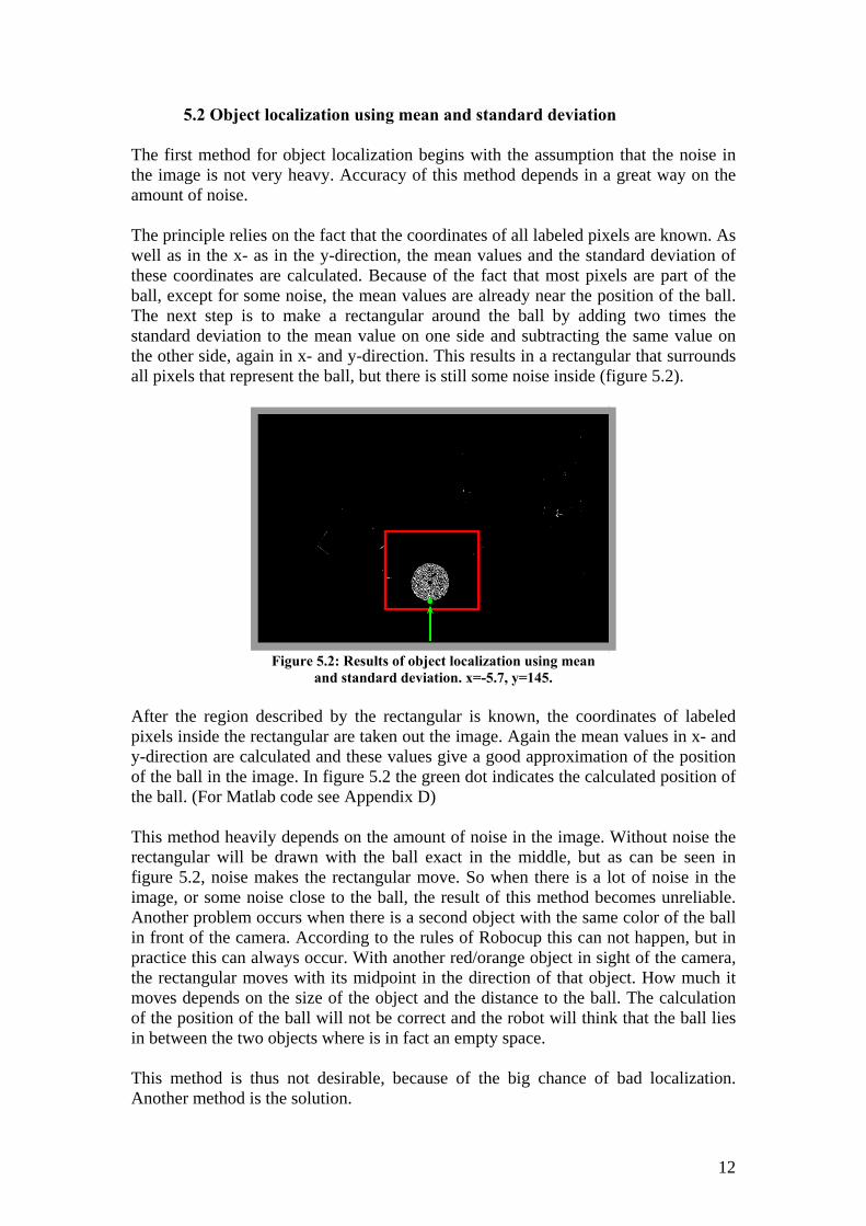
5.2 Object localization using mean and standard deviation The first method for object localization begins with the assumption that the noise in the image is not very heavy. Accuracy of this method depends in a great way on the amount of noise. The principle relies on the fact that the coordinates of all labeled pixels are known. As well as in the x- as in the y-direction, the mean values and the standard deviation of these coordinates are calculated. Because of the fact that most pixels are part of the ball, except for some noise, the mean values are already near the position of the ball. The next step is to make a rectangular around the ball by adding two times the standard deviation to the mean value on one side and subtracting the same value on the other side, again in x- and y-direction. This results in a rectangular that surrounds all pixels that represent the ball, but there is still some noise inside (figure 5.2).

Figure 5.2: Results of object localization using mean

and standard deviation. x=-5.7, y=145. After the region described by the rectangular is known, the coordinates of labeled pixels inside the rectangular are taken out the image. Again the mean values in x- and y-direction are calculated and these values give a good approximation of the position of the ball in the image. In figure 5.2 the green dot indicates the calculated position of the ball. (For Matlab code see Appendix D) This method heavily depends on the amount of noise in the image. Without noise the rectangular will be drawn with the ball exact in the middle, but as can be seen in figure 5.2, noise makes the rectangular move. So when there is a lot of noise in the image, or some noise close to the ball, the result of this method becomes unreliable. Another problem occurs when there is a second object with the same color of the ball in front of the camera. According to the rules of Robocup this can not happen, but in practice this can always occur. With another red/orange object in sight of the camera, the rectangular moves with its midpoint in the direction of that object. How much it moves depends on the size of the object and the distance to the ball. The calculation of the position of the ball will not be correct and the robot will think that the ball lies in between the two objects where is in fact an empty space. This method is thus not desirable, because of the big chance of bad localization. Another method is the solution.

12

5.3 Object localization using variance The method described in the previous section is sufficient when an image is not heavily disturbed by noise and when there is only one object in sight of the camera. To make the vision system more robust, another method is needed. A solution is found in the use of the variance. At first the y-position of the ball will be calculated and the x-position can be obtained in a similar way. For every row of pixels in the image, the variance can be calculated what is an indication for the number of labeled pixels in that row. In rows with many labeled pixels, the variance is significantly higher than in rows with just a couple of labeled pixels. At this point a list with for every row a value for the variance is known. Every value that is higher than 15 times the minimum variance is indicated in a new list with the value one. Now a list appears with a length equal to the height of the image with ones at each place that represent a row with a high amount of labeled pixels. The next step is to search for continuous parts in the list because that can be an indication for an object. This is done by going through the whole list and when two successive row numbers are less than 10 spaces apart, they are connected with ones. From this a list appears with again zeros and ones where large areas in the image are recognized as a dense part of ones. It can occur that there is more than one dense part of ones in the list, due to noise or another object with the same color. To prevent the robot from going somewhere far away without reason, the object nearest to the robot must be indicated as the ball. Therefore it is necessary to find the biggest part of ones in the list and indicate this part as the ball. The y-position of the ball is the lowest point in this part in the list. The code is included in Appendix D. For the x-position the same routine must be followed, but instead of rows the columns must be evaluated. The x-position is the mean of the column numbers indicated as the biggest object. In figure 5.2 the results of this method are shown.

Figure 5.2: Result of object localization using variance.

x=-6.5, y=146

13

As can be seen at the sides of figure 5.2, the lists with the dense parts of ones are very accurate and so is the calculation of the position (green spot). The big advantage of this method over the previous method is the insensitivity for noise and the recognition of various objects in the image. Therefore the localization of the ball is more robust than the previous method. Nevertheless there is one disadvantage, and that is the loss of speed. In table 5.2 can be seen what the difference is in time delay between the two localization methods for the example. The method that uses the variance is a bit slower, but the results of localization are a lot better, so this method must be considered best.

Table 5.2: Time delays for different localization methods Localization method Time delay [s] Mean/standard deviation 0.091 Variance 0.151

5.4 Object localization in front of the robot Now the position of the ball in the image is known, this information can be used to calculate the position of the ball in front of the robot. This is of course dependent on the position and the angle of the camera on top of the robot and also the field of sight is an important factor. In figure 5.3 the field of sight and the camera angle are visualized. The field of sight is also dependent on the type of camera that is used.

d

"

h

Figure 5.3a: Side view of the field of sight. (α=camera angle)

r

d

Figure 5.3b: Top view of the field of sight.

The r- and d- coordinates in figure 5.3 are very much related to the x- and y-coördinates in the images captured by the camera. An object that is far away from the camera, thus with a large value for d, will appear at the top of the image, so the value for y will also be large. The r-coordinate has a similar relation with the x-coordinate. An r-value of zero indicates an object right in front of the robot, so the x-value in the

14

image is also zero. The height (h) of an object is not important, because the object localization method detects the position of an object at the lowest point.

5.4.1 XY / RD relation Because the relation between the rd-values and the xy-values is dependent on the camera angle, camera height and type of camera, the conversion from xy- to rd-values must be considered separately for every case. When a simple webcam (figure 5.4) is used at a height of 65cm and pointed at an angle of 65°, the maximum value for d is about 6m and the minimum value is 70cm. An object lies in the middle of the image at a distance of 1.50m, so the relation between the rd- and xy-values is not linear as can be seen in figure 5.3a. In this example, the camera has a resolution of 320x240 pixels and a quadratic function for the relation between d and y gives a very good approximation:

Aip

706.108

2

+=yd

With d in cm and y in number of pixels. The maximum and minimum values for r are dependent on the value distance of 1.50m the maximum value for r is 60cm and at a distance omaximum for r is 32cm. Figure 5.3 shows that the relation betweenmaximum of r is linear and so is the relation between x and r, so tbecomes:

xdr *120

3235.0*)70( +−=

With d and r in cm, x in number of pixels. This is just a rough approximation that can be calculated very easilydifferent vision setup. The number of measurements can be increasedrelations between the xy- and rd-values.

Figure 5.4: tec Megacam.

5.1

of d. At a f 70cm, the d and the his relation

5.2

for every for better

15

6. Vision implementation in Matlab/Simulink All steps towards a vision system that can recognize the ball in a Robocup environment are made. The only thing left to do is linking together all steps to one system. The platform on which this is done is Matlab. It is not the ideal platform to run a vision system on, but it is sufficient to show that this method works. The best option for creating a vision system is the programming language C or C++. These languages are a lot faster than Matlab, so the frequency with which images can be analyzed is a lot higher. This report will not take C or C++ into account and will focus on the use of Matlab. Simulink will also be discussed as a platform to run this vision system on, but this will turn out to be a disappointment. As said before, a very important factor in a vision system is the frequency with which images can be analyzed. For this system the frequency is dependent on the time it takes to localize the ball in an image. Advanced vision systems can reach frequencies of about 30Hz, but for this system a frequency of 10 Hz would be acceptable, because of the use of Matlab. The speed with which a computer can perform calculations is of course dependent on the kind of computer that is used and as a result the frequency of the vision system is restricted, but that influence is left out of consideration.

6.1 Matlab In Matlab version 7.0.4, a new toolbox is introduced. This toolbox is named the ‘image acquisition toolbox’ and it is used to acquire images from external video devices [11]. In previous versions of Matlab a standalone file had to be made to make Matlab communicate with a video device, but with the new toolbox that is not necessary. The basis of a vision system is color definition. This has to be done only once, by running the m-file in Appendix B. When this is done, the color matrix is known and the vision system is ready to go. A video device can easily be connected to Matab using the ‘videoinput’-function (Appendix A). This function makes it possible to assign a variable as a video input. Image processing can not be performed on a video input, so single frames have to be extracted from the video with a frame grabber. A so-called snapshot is taken out of the video input and this single picture is used for pixel labeling and object localization. When the coordinates of the ball in this image are known, the next snapshot can be taken out of the video input and the position of the ball can be calculated once again.

6.1.1 Results The frequency of this system can be calculated by adding all time delays caused by the different actions. Color definition and the connection with the video device can be left out of consideration, because this has to be done before the vision system starts. The time delays caused by the remaining actions are calculated for the camera in figure 5.4 with a resolution of 320x240 pixels. The results are put in table 6.1.

16

Table 6.1: Time delays for all actions with a resolution of 320x240 pixels. Action Time delay (s) Frame grabber 0.0574 Position calculation ( Eq. 5.1 / 5.2 ) 0.0 Pixel interval = 1 Pixel labeling 0.0334 Object localization 0.0972 Total 0.188 Pixel interval = 3 Pixel labeling 0.00764 Object localization 0.0421 Total 0.107 Pixel interval = 5 Pixel labeling 0.00183 Object localization 0.0369 Total 0.0961 As can be seen in table 6.1, the frame grabber and the object localization are the main contributors in the total time delay. It takes some time in Matlab to grab a frame out of the video input an there is no solution for this problem, because this is the only way to get a frame of a video input. The time delay caused by the object localization can be shortened by choosing another localization method, but that will influence the accuracy. The solution for this problem, and probably also the solution for the time delay of the frame grabber, is the programming language C or C++. All the other actions will go a lot faster too, so the frequency would increase very much, but this will not be discussed in this report. Tabel 6.1 shows that for the complete system a frequency can be reached of 10.4Hz with a pixel interval of 5. The frequency of 9.35Hz that is reached with a pixel interval of 3 is not that much lower and the smaller pixel interval results in a more accurate object recognition as seen in section 4.3.2. Therefore the pixel interval of 3 is preferred over the pixel interval of 5 and the frequency of this vision system becomes 9.35Hz. This frequency is of course not a constant factor in the system, because of fluctuations in computer usage.

6.2 Simulink Because the frequency that is reached in Matlab is not as high as expected, a closer look at Simulink is the next option. Version 7.0.4 contains the image acquisition toolbox with a ‘video input’-block [11]. This block has the same function as the ‘videoinput’-function in Matlab. This block sends out 3 matrices with the values of red, green and blue for each pixel. With this information the position of the ball can be calculated. There are no blocks with a ball-recognition function, so a solution must be found. The first solution is an embedded m-file. This is a normal Matlab m-file inside the simulink model, so the same Matlab code as before can be used. There is however a problem with the usage of parameters in the embedded m-file. These parameters can only be 2dimensional and the color matrix is 3dimensional. This problem can be solved by transforming the color matrix into a 2D matrix, but the size of this matrix becomes extremely large, namely 256x256^2. Simulink can not handle matrices of this size and the program will crash before running the model.

17

Another option is the ‘block processing’-block in the ‘video and image processing toolbox’ [11]. This block can divide the matrices into pixels and a 3D-lookup table with the color matrix can be used for pixel labeling. After the action performed on the pixels, the ‘block processing’-block puts them all together into one matrix. The output matrix can be used of object localization with the use of an embedded m-file. This method works, but the speed with which images are analyzed is very low. The frequency drops even under one, so this is not very useful. There are no other methods found to implement this vision system in Simulink, so it can be said that Simulink is no good option for now. Perhaps with the implementation of c-codes in Simulink these problems will not occur, but that is not taken into account.

18

7. Conclusion The progress in the world of robotics has increased very much over the last few years. A couple of years ago the robots in the Robocup competition relied on their laser- and infrared-senors, but nowadays they are equipped with advanced vision systems based on color recognition. Those camera based vision systems are getting faster and faster and the frequency with which they can analyze images is already 30Hz. A complete vision system has to recognize all important elements in a Robocup environment, so a complete system will be more complex than the system described in this report. However, the basics for every object are the same. For good vision systems a couple of processes are very important. Color definition and color recognition are the basis, because without knowing the difference between colors, there can be no object recognition. When colors are recognized in the image, the right area has to be recognized as an object and the position of this object must be calculated. With this knowledge the position of the object in front of the robot is not difficult to obtain. The examinations done in this report resulted in a system to recognize the ball in front of the robot with a frequency of 9.35Hz. This is significantly lower than the advanced systems and also a bit lower than the expected 10Hz. The difference is mainly due to the platform on which the system is built upon. This report focuses on the implementation in Matlab, and that platform is not ideal for implementing a vision system because of the relative low speed of loops. The solution can be found in the more advanced programming languages C and C++.

19

8. References [1] J. Gonzalez, A. Ollero, A. Reina, ‘Map building for a mobile robot equipped

with a 2D laser rangefinder’, IEEE Int. Conf On Robotics and Automation, pp [2] M.J.Chantler, ‘Detection and tracking of returns in sector-scan sonar image

sequences’ [3] James Bruce, Tucker Balch, Manuela Veloso, ‘Fast and Inexpensive Color

Image Segmentation for Interactive Robots’ [4] A. Bonarini, P. Aliverti, M. Lucioni, "An omni-directional sensor for fast

tracking for mobile robots", Proc. of the 1999 IEEE Instrumentation and measurement Technology Conference (IMTC99), IEEE Computer Press, Piscataway, NJ, pp. 151-157

[5] Robocup website, http://www.robocup.org, 2005 [6] Tim Morris , ‘Computer vision and image processing’, Basingstoke : Palgrave

Macmillan, 2004 [7] JAMES M. KASSON, WIL PLOUFFE, ‘An Analysis of Selected Computer

Interchange Color Spaces’ [8] Mathworks Matlab Image Processing function list,

http://www.mathworks.com/products/image/functionlist.html, 2005 [9] Mathworks Matlab Image Processing demos,

http://www.mathworks.com/products/image/demos.jsp, 2005 [10] I. Patras, ‘Object-based video segmentation with region labeling’, Delft 2001 [11] Mathworks Matlab Image Acquisition Toolbox overview,

http://www.mathworks.com/products/imaq/

20

Appendix A Explanation of Matlab functions For more details, see Matlab help. Roipoly-function region = roipoly(img) Use roipoly to select a polygonal region of interest within an image. roipoly returns a binary image that you can use as a mask for masked filtering. region = roipoly(img) returns the region of interest selected by the polygon described by the user. Videoinput-function Getsnapshot-function vid = videoinput('winvideo'); preview(vid); img = getsnapshot(vid) ; Vid becomes the name of the video input. The string ‘winvideo’ defines the device adaptor vid is associated with. For the use of most common cameras, the value ‘winvideo’ can be used. Valid values can be determined by using the imaqhwinfo function. To use the getsnapshot-function it is necessary to perform the preview function first. This function gives the images captured by the camera device. By using getsnapshot, a frame can be taken out of the preview.

21

Appendix B Matlab code for color definition clear all colors = [] ; %%%%%%%%%%%%%%%%%%%%%%%%%%%%%%%%%%%%% % Set ranges for H and S. h = 0.03:0.002:0.13 ; s = 0.7:0.002:1 ; %%%%%%%%%%%%%%%%%%%%%%%%%%%%%%%%%%%%% % Make a column so that every combination % of H, S and V is possible. ss = [] ; for i = 1:length(h) hh((i-1)*length(s)+1:i*length(s),1) = h(i) ; ss = [ss ; s'] ; end %%%%%%%%%%%%%%%%%%%%%%%%%%%%%%%%%%%%% % Define the range for V and make a matrix % of the same size as hh and ss. v = repmat([0.64:0.002:1],[length(hh),1],1) ; colors(:,:,1) = repmat(hh,[1,length(v(1,:))],1) ; colors(:,:,2) = repmat(ss,[1,length(v(1,:))],1) ; colors(:,:,3) = v ; %%%%%%%%%%%%%%%%%%%%%%%%%%%%%%%%%%%%% % Transform the HSV values to RGB values and % let the values range from 1 to 256. colors = hsv2rgb(colors) ; colors = round(colors*255)+1 ; %%%%%%%%%%%%%%%%%%%%%%%%%%%%%%%%%%%%% % Put all defined colors in a 3D-matrix % named clrs. clrs = repmat(0,[256,256],256) ; s = size(colors) ; for i = 1:s(1) for j = 1:s(2) clrs(colors(i,j,1),colors(i,j,2),colors(i,j,3)) = 1 ; end end %%%%%%%%%%%%%%%%%%%%%%%%%%%%%%%%%%%%% % Manual color definition %%%%%%%%%%%%%%%%%%%%%%%%%%%%%%%%%%%%% % color = imread('HSV colors.bmp') ; % figure(1) % imshow(color) % % regions(:,:,n) = roipoly(color) ; % img = rgb2hsv(color) ; % % H = img(:,:,1) ; % S = img(:,:,2) ; % V = img(:,:,3) ; % % h = H(regions(:,:,n)) ; % s = S(regions(:,:,n)) ; % v = repmat([0.64:0.002:1],[length(h),1],1) ; % % hh = repmat(h,[1,181],1) ; % ss = repmat(s,[1,181],1) ; % % colors(:,:,1) = repmat(hh,[1,length(v(1,:))],1) ; % colors(:,:,2) = repmat(ss,[1,length(v(1,:))],1) ; % colors(:,:,3) = v ; % % colors = hsv2rgb(colors) ; % colors = round(colors*255)+1 ; % % clrs = repmat(0,[256,256],256) ; % s = size(colors) ; % for i = 1:s(1) % for j = 1:s(2) % clrs(colors(i,j,1),colors(i,j,2),colors(i,j,3)) = 1 ; % end % end %%%%%%%%%%%%%%%%%%%%%%%%%%%%%%%%%%%%%

22

Appendix C Matlab code for pixel labeling %%%%%%%%%%%%%%%%%%%%%%%%%%%%%%%%%%%%% % Define the pixel interval. pix = 1 ; p = round(pix/2) ; %%%%%%%%%%%%%%%%%%%%%%%%%%%%%%%%%%%%% % Import the image for pixel labeling % (in the final version this is a videoinput). img = imread('robocup2.bmp') ; img = double(img) ; h = size(img,1) ; w = size(img,2) ; %%%%%%%%%%%%%%%%%%%%%%%%%%%%%%%%%%%%% % Set the size of the segmented image % and perform pixel labeling. segmented_image = repmat(0,[floor((h-pix)/pix+1),floor((w-pix)/pix+1)],1) ; for y = p : pix : floor((h-pix)/pix)*pix+p ; for x = p : pix : floor((w-pix)/pix)*pix+p ; c = clrs(img(y,x,1) + 1,img(y,x,2) + 1,img(y,x,3) + 1) ; segmented_image((y-p)/pix+1,(x-p)/pix+1) = c ; end end

23

Appendix D Matlab code for object recognition Using variance %%%%%%%%%%%%%%%%%%%%%%%%%%%%%%%%%%%%% varx = [] ; vary = [] ; %%%%%%%%%%%%%%%%%%%%%%%%%%%%%%%%%%%%% % Calculate the variance in x and y direction. vx = var(segmented_image(:,:)) ; vy = var(segmented_image(:,:)') ; %%%%%%%%%%%%%%%%%%%%%%%%%%%%%%%%%%%%% % If labeled pixels are found, % Calculate the position of the ball. if length(find(vx))>0 && length(find(vy))>0 s = size(segmented_image) ; w = s(2) ; h = s(1) ; for i = 1 : w ; varx(i) = (vx(i) > (min(vx(find(vx)))*15)) ; end for i = 1 : h ; vary(i) = (vy(i) > (min(vy(find(vy)))*15)) ; end f = find(varx) ; ff = [] ; for i = 1 : length(f)-1 ; if (f(i+1) > f(i)+10) ; ff = [ff f(i) f(i+1)] ; end end ff = [ff f(length(f))] ; ff = [f(1) ff]; fx = [] ; for i = 1 : 2 : length(ff)-1 fx = [fx ff(i+1)-ff(i)] ; end m = max(fx) ; m = find(fx==m) ; rx = ff(2*m-1) : ff(2*m) ; xball = zeros(size(varx)) ; xball(rx) = 1 ; xbal = mean(rx) ; f = find(vary) ; ff = [] ; for i = 1 : length(f)-1 ; if (f(i+1) > f(i)+10) ; ff = [ff f(i) f(i+1)] ; end end ff = [ff f(length(f))] ; ff = [f(1) ff]; fy = [] ; for i = 1 : 2 : length(ff)-1 fy = [fy ff(i+1)-ff(i)] ; end m = max(fy) ; m = find(fy==m) ; ry = ff(2*m-1) : ff(2*m) ; yball = zeros(size(vary)) ; yball(ry) = 1 ; ybal = max(ry) ; else end %%%%%%%%%%%%%%%%%%%%%%%%%%%%%%%%%%%%%

24

Using mean and standard deviation %%%%%%%%%%%%%%%%%%%%%%%%%%%%%%%%%%%%% if length(yball) > 0 && length(xball) > 0 [yball,xball] = find(segmented_image(:,:)) ; ymean = mean2(yball) ; ystd = std2(yball) ; yb = round(ymean - 2*ystd) - ((ymean - 2*ystd) < 1 )*((ymean - 2*ystd)+1) : 1 : round(ymean + 2*ystd) - ((ymean + 2*ystd) > h )*((ymean + 2*ystd)-h) ; xmean = mean2(xball) ; xstd = std2(xball) ; xb = round(xmean - 2*xstd) - ((xmean - 2*xstd) < 1 )*((xmean - 2*xstd)+1) : 1 : round(xmean + 2*xstd) - ((xmean + 2*xstd) > w )*((xmean + 2*xstd)-w) ; [yball,xball] = find(segmented_image(yb,xb)) ; yball = h - (max(yball) + min(yb))*pix ; xball = - (0.5*w - ((mean2(xball) + min(xb))*pix)) ; else end %%%%%%%%%%%%%%%%%%%%%%%%%%%%%%%%%%%%%

25