basic tutorial to ltex programming · basic tutorial to latex programming ... ii. latex ? latex,...

LATEX programminghttps://www.latex-project.org/

Basic tutorial to LATEX programming

Sébastien LE ROUX [email protected]

INSTITUT DE PHYSIQUE ET DE CHIMIE DES MATÉRIAUX DE STRASBOURG,DÉPARTEMENT DES MATÉRIAUX ORGANIQUES,

23 RUE DU LOESS, BP43,F-67034 STRASBOURG CEDEX 2, FRANCE

APRIL 5, 2018

https://www.latex-project.org/

mailo:[email protected]

Contents

Contents ii

1 LATEX ? 1

1.1 WYSIWYG vs. LATEX . . . . . . . . . . . . . . . . . . . . . . . . . . . . . . . . . . . . 11.2 Installing LATEX . . . . . . . . . . . . . . . . . . . . . . . . . . . . . . . . . . . . . . . 2

1.2.1 Linux . . . . . . . . . . . . . . . . . . . . . . . . . . . . . . . . . . . . . . . . 21.2.2 Mac . . . . . . . . . . . . . . . . . . . . . . . . . . . . . . . . . . . . . . . . . 31.2.3 Windows . . . . . . . . . . . . . . . . . . . . . . . . . . . . . . . . . . . . . . 3

1.3 Before running LATEX . . . . . . . . . . . . . . . . . . . . . . . . . . . . . . . . . . . . 31.3.1 WYSIWYG-like tools for LATEX . . . . . . . . . . . . . . . . . . . . . . . . . . 31.3.2 LATEX editor . . . . . . . . . . . . . . . . . . . . . . . . . . . . . . . . . . . . . 41.3.3 How to install manually a package for LATEX . . . . . . . . . . . . . . . . . . . 4

2 LATEX - the first step 9

2.1 Structure of the document . . . . . . . . . . . . . . . . . . . . . . . . . . . . . . . . . . 92.1.1 The document class . . . . . . . . . . . . . . . . . . . . . . . . . . . . . . . . . 92.1.2 The preamble section . . . . . . . . . . . . . . . . . . . . . . . . . . . . . . . . 112.1.3 The main body of the manuscript . . . . . . . . . . . . . . . . . . . . . . . . . 11

2.2 Running LATEX . . . . . . . . . . . . . . . . . . . . . . . . . . . . . . . . . . . . . . . 122.2.1 The tools that you will need . . . . . . . . . . . . . . . . . . . . . . . . . . . . 122.2.2 The compilation process . . . . . . . . . . . . . . . . . . . . . . . . . . . . . . 12

3 LATEX essentials 15

3.1 Commands . . . . . . . . . . . . . . . . . . . . . . . . . . . . . . . . . . . . . . . . . 153.2 Environments . . . . . . . . . . . . . . . . . . . . . . . . . . . . . . . . . . . . . . . . 163.3 Packages . . . . . . . . . . . . . . . . . . . . . . . . . . . . . . . . . . . . . . . . . . 193.4 Files . . . . . . . . . . . . . . . . . . . . . . . . . . . . . . . . . . . . . . . . . . . . . 19

4 My first LATEX document 21

4.1 Preparing the preamble . . . . . . . . . . . . . . . . . . . . . . . . . . . . . . . . . . . 214.2 Writing the manuscript . . . . . . . . . . . . . . . . . . . . . . . . . . . . . . . . . . . 23

4.2.1 Writing text . . . . . . . . . . . . . . . . . . . . . . . . . . . . . . . . . . . . . 234.2.2 Title, authoring and abstract . . . . . . . . . . . . . . . . . . . . . . . . . . . . 264.2.3 Organizing your document . . . . . . . . . . . . . . . . . . . . . . . . . . . . . 264.2.4 Inserting a math equation . . . . . . . . . . . . . . . . . . . . . . . . . . . . . . 294.2.5 Inserting a table . . . . . . . . . . . . . . . . . . . . . . . . . . . . . . . . . . . 30

i

4.2.6 Inserting an image . . . . . . . . . . . . . . . . . . . . . . . . . . . . . . . . . 314.2.7 Inserting a list / enumeration . . . . . . . . . . . . . . . . . . . . . . . . . . . . 334.2.8 Inserting a reference . . . . . . . . . . . . . . . . . . . . . . . . . . . . . . . . 344.2.9 Inserting web links and emails . . . . . . . . . . . . . . . . . . . . . . . . . . . 354.2.10 Inserting a bibliography . . . . . . . . . . . . . . . . . . . . . . . . . . . . . . 35

5 Spell checking 39

5.1 Using the command line . . . . . . . . . . . . . . . . . . . . . . . . . . . . . . . . . . 395.2 Using Texmaker . . . . . . . . . . . . . . . . . . . . . . . . . . . . . . . . . . . . . . . 40

6 LATEX advantages and drawbacks 43

7 Examples 47

7.1 Title and authors . . . . . . . . . . . . . . . . . . . . . . . . . . . . . . . . . . . . . . 477.1.1 RevTex 4.1 - "revtex4-1" . . . . . . . . . . . . . . . . . . . . . . . . . . . . . . 477.1.2 American Chemical Society "achemso" . . . . . . . . . . . . . . . . . . . . . . 487.1.3 Elsevier "elsarticle" . . . . . . . . . . . . . . . . . . . . . . . . . . . . . . . . . 497.1.4 Institute Of Physics "iopart" . . . . . . . . . . . . . . . . . . . . . . . . . . . . 50

7.2 Tables and figures . . . . . . . . . . . . . . . . . . . . . . . . . . . . . . . . . . . . . . 517.3 Equations . . . . . . . . . . . . . . . . . . . . . . . . . . . . . . . . . . . . . . . . . . 53

8 Partial glossary 55

8.1 Useful commands . . . . . . . . . . . . . . . . . . . . . . . . . . . . . . . . . . . . . . 558.1.1 In text mode . . . . . . . . . . . . . . . . . . . . . . . . . . . . . . . . . . . . 558.1.2 In math mode . . . . . . . . . . . . . . . . . . . . . . . . . . . . . . . . . . . . 56

8.2 Useful environments . . . . . . . . . . . . . . . . . . . . . . . . . . . . . . . . . . . . 57

9 Error messages 59

9.1 LATEX errors . . . . . . . . . . . . . . . . . . . . . . . . . . . . . . . . . . . . . . . . . 599.2 TEX errors . . . . . . . . . . . . . . . . . . . . . . . . . . . . . . . . . . . . . . . . . . 61

10 Some useful links 63

ii

LATEX ?

LATEX, shortcut for ’Lamport TEX’, is a document markup language invented by Leslie Lamportin 1983. The purpose of LATEX is to simplify the utilization of the word processor TEX devel-oped by Donald Knuth since 1977.With typical word processors such as Microsoft Word and LibreOffice Writer, called WYSI-

WYG editors "What You See Is What You Get", one can immediately visualize the formattedtext and the final shape of the document on the screen.In LATEX the writer uses plain text (as opposed to formatted text), relying on markup taggingconventions to:

• define the general structure of a document (such as article, book, and letter).

• stylize text throughout a document (such as bold and italic).

• insert objects in the document (such as tables and figures).

• add citations and cross-referencing.

A TEX distribution such as TeX Live or MiKTeX is used to produce an output file (such as PS,PDF or DVI) suitable for printing or digital distribution.

The latest version of LATEX is called LATEX 2ε.

Many ideas in this HowTo where inspired by the very good book "LATEX par la pratique" (inFrench) by Christian Rolland [1] ...

... and many others by the LATEX Wikibooks: https://en.wikibooks.org/wiki/LaTeX

1.1 WYSIWYG vs. LATEX

LATEX being a programming language it is required to learn it, or at least a part of it, whichscares most of the potential candidates to use it.

1


https://www.tug.org/texlive/

http://miktex.org/

https://en.wikibooks.org/wiki/LaTeX

Chapter 1. LATEX ? 2

Using a WYSIWYG editor you can visualize the result of your work immediately. With LATEXfew steps are required to obtain the final manuscript using the source file(s) in TEX language.The sequence of these steps is called compilation, and the compilation process can slightlychange from one case to another.

1.2 Installing LATEX

1.2.1 Linux

To install TEX and LATEX 2ε on Linux you can simply use your favorite package manager(Yumex, Synaptic ...), see bellow for a list of packages.You can also use the command line, remember that you need to be logged in a administrator.To install the complete TeX Live distribution (∼ 1.5Go):

• RedHat based Linux distributions:

user@localhost ~]$ yum install texlive-scheme-full

• Debian based Linux distributions:

user@localhost ~]$ sudo apt-get install texlive-full

To install the minimal Tex Live distribution on RedHat based Linux use:

user@localhost ~]$ yum install texlive

Afterwards the following commands ensure that you will install on your computer all thepackages required to produce the examples proposed in this HowTo, many of which mightalready be installed by the previous command.

• Math and tables:

~]$ yum install texlive-amstex texlive-tabls texlive-multirow

• Images and graphics:

~]$ yum install texlive-graphviz texlive-xcolor

• Scientific editors:

~]$ yum install texlive-revtex4 texlive-achemso

~]$ yum install texlive-iopart tetex-elsevier

2

3 1.3. Before running LATEX

• Bibliography:

~]$ yum install texlive-bibtex

• Others:

~]$ yum install texlive-hyperref texlive-pslatex texlive-babel

1.2.2 Mac

You need to install the MacTeX distribution:

• Complete MacTeX package (∼ 2Go): https://tug.org/mactex/mactex-download.html

• Smaller MacTeX distribution: https://tug.org/mactex/morepackages.html

1.2.3 Windows

The best choice is probably to install the MiKTeX distribution which is an up-to-date imple-mentation of TEX, LATEX and related programs for Windows:

• Internet installer: http://miktex.org/download

Alternatively you can install the TeX Live distribution:

• Internet installer: https://www.tug.org/texlive/acquire-netinstall.html

• Obtain TeX Live on DVD: http://https://www.tug.org/texlive/acquire-dvd.html

1.3 Before running LATEX

1.3.1 WYSIWYG-like tools for LATEX

To help you start you can install some tools that offer a WYSIWYG interface for LATEX:

• GNU TeXmacs: http://www.texmacs.org/

• BaKoMa TEX: http://www.bakoma-tex.com/

Using these softwares you can prepare your LATEX manuscript in a Microsoft Word or Libre-Office Writer kind of way, however they are limited and the source file they produce, if yougenerate some errors, and you will, is usually complicated to read.

3

https://tug.org/mactex/

https://tug.org/mactex/mactex-download.html

https://tug.org/mactex/morepackages.html

http://miktex.org/download

https://www.tug.org/texlive/acquire-netinstall.html

http://https://www.tug.org/texlive/acquire-dvd.html

http://www.texmacs.org/

http://www.bakoma-tex.com/


1.3.2 LATEX editor

To start working you need to pick a text editor, if your OS is Microsoft Windows remember touse a "Unix Line Endings" editor. Indeed many Windows-based text editors add a particularsymbol at the end of each line to signify that the line is breaking, and this symbol is messingwith LATEX. Among the editors that can be used:

• The basic editors:

– GNU Emacs

– gVim

• The tools dedicated to LATEX:

– Texmaker see figure [Fig. 1.1]

– TEXnicCenter

– TeXworks

– TeXstudio

Hereafter I will use few examples from Texmaker, an opensource multiplateform (Linux, Mac,Windows) software that provides a user interface with spell-checking (see ??), help to manyLATEX commands and a PDF reader.

1.3.3 How to install manually a package for LATEX

Add-on features for LATEX are known as packages. Dozens are pre-installed with LATEX and canbe used immediately. They should all be stored in sub-directories of texmf/tex/latex namedafter each package. The directory name "texmf" stands for "TEX and METAFONT".A package is a file or collection of files containing extra LATEX commands and programmingwhich add new styling features or modify those already existing. There are two main file typesdelivered by packages:

• class files with .cls extension

• style files with .sty extension

When you try to typeset a document which requires a package which is not installed on yoursystem, LATEX will warn you with an error message that it is missing [see 9]. Most LATEXinstallations come with a large set of pre-installed style packages, so you can use the packagemanager of the TEX distribution or the one on your system to manage them. But many more areavailable on the net. The main place to look for style packages on the Internet is ComprehensiveTEX Archive Network, CTAN. Once you have identified a package you need that is not in yourdistribution, use the search engines of any CTAN server to find it. Download and follow thisprocedure to install it (after opening the archive):

4

https://www.gnu.org/software/emacs/

http://www.vim.org/

http://www.xm1math.net/texmaker/index_fr.html

http://www.texniccenter.org/

http://tug.org/texworks/

https://sourceforge.net/projects/texstudio/

http://ctan.org


Figure 1.1 The main window of the Texmaker editor

1. Extract the files of the package: run LATEX on the *.ins file, ex:

• For Linux / Mac:

user@localhost ~]$ latex package.ins

• For Windows open the *.ins using Texmaker and run a "Quick Build" [see 2.2.2]

2. Create the documentation: run LATEX twice on the *.dtx file, ex:

• For Linux / Mac:

user@localhost ~]$ latex package.dtx

user@localhost ~]$ latex package.dtx

• For Windows open the *.dtx using Texmaker and run a "Quick Build" [see 2.2.2]

3. Install the files:

Packages installed manually should always be placed in your "local" directory, not in thedirectory tree containing all the pre-installed packages. This is done to prevent your newpackage to accidentally overwrite files in the main TEX directory.

5


The folder to look for should probably be called texmf/ or texmf-local/ and its loca-tion depends on your operating system:

• Linux: $HOME/texmf/

• Mac (MacTeX): /Users/username/Library/texmf/

• Windows (MikTeX): any folder registered as a user-managed texmf directory

The "right place" sometimes causes confusion, the "right place" for a LATEX .sty file is asuitably-named sub-directory of texmf/tex/latex/ "Suitably-named" means sensible,meaningful and probably short.Often there is just a .sty file to move, but for complex packages there may be more,and they may belong in different locations. For example, new BibTeX packages or fontpackages will typically have several files to install. This is why it is a good idea to createa sub-directory for the package rather than dump the files into misc along with otherunrelated stuff. In any case read the documentation to find out if there is a special orpreferred location to move them to.

Table 1.1 Where to put the files from the packages

Type Directory (in texmf/ or texmf-local/) Description

.afm fonts/afm/foundry/typeface Adobe Font Metrics for Type 1 fonts

.bst bibtex/bst/packagename BibTeX style

.cls tex/latex/base Document class file

.dvi doc package documentation

.enc fonts/enc Font encoding

.fd tex/latex/mfnfss Font Definition files for METAFONT fonts

.fd tex/latex/psnfss Font Definition files for PostScript Type 1 fonts

.map fonts/map Font mapping files

.mf fonts/source/public/typeface METAFONT outline

.pdf doc Package documentation

.pfb fonts/type1/foundry/typeface PostScript Type 1 outline

.sty tex/latex/packagename Style file: the normal package content

.tex doc TEX source for package documentation

.tex tex/plain/packagename Plain TEX macro files

.tfm fonts/tfm/foundry/typeface TEX Font Metrics for METAFONT and Type 1 fonts

.ttf fonts/truetype/foundry/typeface TrueType font

.vf fonts/vf/foundry/typeface TEX virtual fontsothers tex/latex/packagename Other types of file unless instructed otherwise

6


4. Update your index:

Run your TEX indexer program to update the package database. This program comes withevery version of TEX and has various names depending on the LATEX distribution you use:

• Linux - TeX Live: texhash

user@localhost ~]$ texhash

• Mac - MacTeX does the job for you.

• Windows - MiKTeX:

– Windows XP through 7: Start menu → All Programs → MiKTeX → Settings

– Windows 8: use the keyword Settings and choose the option of Settings withthe MiKTeX logo.

In Settings menu choose the first tab and click on Refresh FNDB-button, after thatjust verify by clicking ’OK’.

7

LATEX - the first step

2.1 Structure of the document

In the most simple case the structure of a LATEX document is as follow:

\documentclass{article}

% Some (important) information here

\begin{document}

Science is great, I love it !

\end{document}

=⇒ the document class - [see 2.1.1]

=⇒ the preamble section - [see 2.1.2]

=⇒ the article starts here

the main body section - [see 2.1.3]

=⇒ the article ends here

The LATEX file is a simple text file with the *.tex extension.

2.1.1 The document class

The document class is the first line of your LATEX file, it is a command that tells LATEX whichtype of document you are going to write, among the default choices provided you can find:

• letter

• article

• book

• beamer

=⇒ to write a letter

=⇒ to write an article

=⇒ to write a book (like your thesis)

=⇒ to create a presentation

9

Chapter 2. LATEX - the first step 10

On the document class declaration line you can also find additional options, or keywords,separated by a coma:

\documentclass[a4paper,12pt]{article}

In this example the first keyword specify the paper layout, the second is used to change thedefault font size in the entire document. 3 different font sizes are available in the book andarticle classes: 10pt, 11pt or 12pt, other are available using packages [see 3.3].For more details about the different keywords or options, please refer the documentation of thecorresponding document class.

Almost all scientific journals provide their own guidelines for LATEX publishing, including thedocument class you need to use, the trick is only, when needed, to download the class from theweb site of the journal and to know how to install it [See 1.3.3]. For example the AmericanPhsyical Society, APS (Phys. Rev., Phys. Rev. Lett. ...) and the American Institute of Physics,AIP (J. Chem. Phys., Appl. Phys. Lett. ...) use the revtex4.1 class:

\documentclass[prb,twocolumn,showkeys,showpacs,english]{revtex4-1}

IOP Publishing (J. Phys.: Cond. Mat., Rep. Prog. Phys. ...) uses the iopart class:

\documentclass[jpcm,twocolumn,english]{iopart}

The American Chemical Society, ACS (J. Am. Chem. Soc., Chem. Mater. ...) uses theachemso class:

\documentclass[jacs,twocolumn,preprint,english]{achemso}

Elsevier journals (J. Non-Cryst. Solids., Comp. Mat. Sci. ...) use the elsarticle class:

\documentclass[jncs,twocolumn,preprint,english,12pt]{elsarticle}

You must have noticed in these examples that a keyword is used to specify the journal it-self inthe options of the document class. Using this keyword LATEX will reproduce the exact layout ofthe scientific journal you are targeting, from the title page to the style of the bibliography.

10

11 2.1. Structure of the document

2.1.2 The preamble section

In this section of the text file you will tell LATEX about all the tools that you need to use:

• Packages = TEX or LATEX extensions that you need to use - [see 3.3]

• Commands = TEX or LATEX commands [see 3.1] that:

– you might need to use in the preamble, these likely depend on the document class.

– you might need to create and use in the preamble - [see 2.1.3]

– you might need to create to use later in the main body of the manuscript - [see 2.1.3]

• Files that can be read by LATEX before processing the rest of the document - [see 3.4]

2.1.3 The main body of the manuscript

In this section you write your manuscript, your truth about science, and whatever comes to yourmind and that can be published !This manuscript section can contain:

• Basic text

• Commands = TEX or LATEX commands [see 3.1] to do many things like:

– Insert a title

– Organize your document

– Insert a math equation

– Insert a table

– Insert an image

– Insert a list (like this one)

– Insert a web link

– Insert a file

– Insert a reference to one of the above

– Insert a bibliographic reference

– Insert a bibliography

=⇒ [see 4.2.2]

=⇒ [see 4.2.3]

=⇒ [see 4.2.4]

=⇒ [see 4.2.5]

=⇒ [see 4.2.6]

=⇒ [see 4.2.7]

=⇒ [see 4.2.9]

=⇒ [see 3.4]

=⇒ [see 4.2.8]

=⇒ [see 4.2.10]

=⇒ [see 4.2.10]

11


2.2 Running LATEX

2.2.1 The tools that you will need

• A text editor

• Working distributions of TEX and LATEX 2ε

• TEX extensions that you might want to use (BibTeX, LaTeX2HTML ...)

2.2.2 The compilation process

For the time being let us consider that you already prepared a TEX file that contains yourmanuscript. This file has to be a basic text file with the extension *.tex, ex: manuscript.tex.To visualize the manuscript requires to build it using this source file that contains the LATEXcommands and the text. This building process is called compilation, depending on your OS andthe tool you are using to prepare your document this can be achieved using 2 methods:

1. Using the command line and the following sequence of commands, to get more familiarwith the command line see [2]:

user@localhost ~]$ latex manuscript

... many blabla


... many blabla

You need to run the command latex twice, the second time is mandatory to cross-checkand update references [see 4.2.8] and citations [see 4.2.10]. The latex command willproduce at least 3 files:

• *.dvi device independent, your manuscript.

• *.log LATEX log journal with information about the last compilation.

• *.aux LATEX auxiliary file.

Afterwards if you want to produce a PostScript, *.ps, use:

user@localhost ~]$ dvips manuscript

And to build a PDF file, use:

user@localhost ~]$ dvipdf manuscript

manuscript is the name of your TEX file without extension, thus without the *.tex.

12

13 2.2. Running LATEX

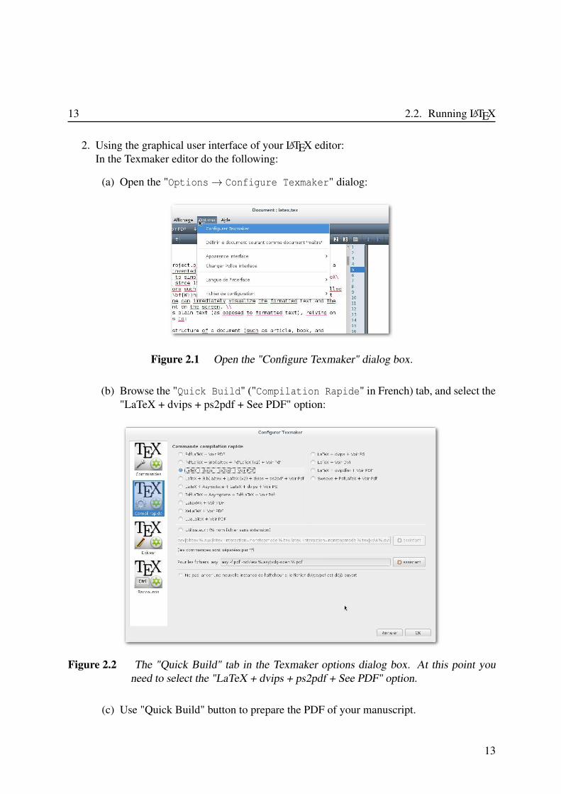
2. Using the graphical user interface of your LATEX editor:In the Texmaker editor do the following:

(a) Open the "Options→ Configure Texmaker" dialog:

Figure 2.1 Open the "Configure Texmaker" dialog box.

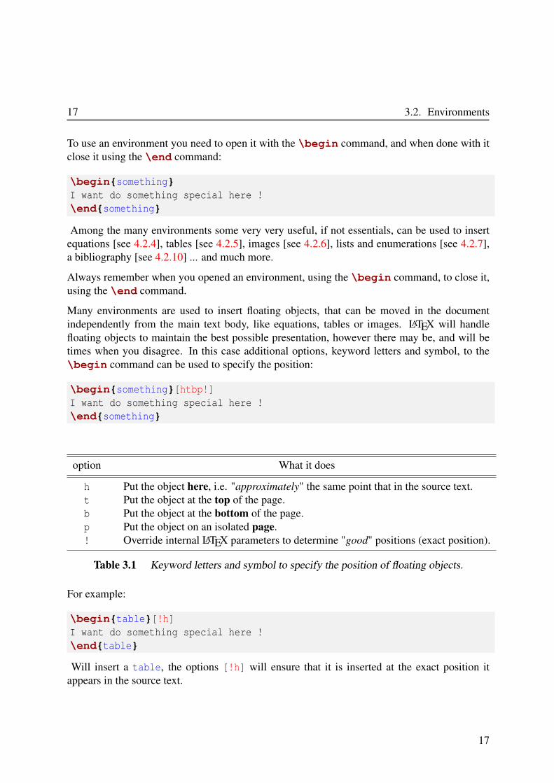
(b) Browse the "Quick Build" ("Compilation Rapide" in French) tab, and select the"LaTeX + dvips + ps2pdf + See PDF" option:

Figure 2.2 The "Quick Build" tab in the Texmaker options dialog box. At this point youneed to select the "LaTeX + dvips + ps2pdf + See PDF" option.

(c) Use "Quick Build" button to prepare the PDF of your manuscript.

13


The compilation is a crucial step in the production of scientific document with LATEX, [see 6,9]for more details.

14

LATEX essentials

3.1 Commands

Since LATEX is a programming language it is fundamental to be able to recognize a command,and you probably already noticed that without commands there is not much that you can do nomatter how powerful LATEX is and how great is the thesis that you want to write.In LATEX a command looks like:

\dosomething

You can also add an option to the command, placed in-between brackets, { }, immediatelyafter the command:

\dosomething{option}

And even more than one:

\dosomething{option 1}{option 2}...

Many, many commands have already been written and can be used to do many, many things,in the following parts of this HowTo I will shortly present some of the most basic, important,fundamental commands that you want to know to be able to write you precious PhD thesis oryour next article using LATEX.However before this, I think that it can be useful to know how to define your own command inLATEX:

\newcommand{\MyCommand}{What-it-does}

Here \newcommand{} is the LATEX command to define a command, the name of this newcommand will be \MyCommand, and it will perform the {What-it-does} operations, exam-

15

Chapter 3. LATEX essentials 16

ple:

\newcommand{\napo}{[(P$_2$O$_5$)$_{1-x}$ (B$_2$O$_3$)$_x$]$_{0.65}$}

As a result, each time that LATEX will find the newly defined \napo command in the document,it will replace it by its content and print: [(P2O5)1−x (B2O3)x]0.65.

You might also want to add options to your command:

\newcommand{\MyCommand}[1]{What-it-does-#1}

The number in red represents the number of options for the command, when defining thecommand the option is referred to using #1, example:

\newcommand{\green}[1]{\textcolor{green}{#1}}

The \textcolor{col}{} is the standard LATEX command to change the font color of thetext between brackets, {}, to the color col. The \green command is simply a shortcut tochange the text color to green, thus each time LATEX will find the \green{something is

written here} command in the document, it will colored the text between brackets, {}, ingreen like this: something is written here.Of course more than one option can be used when defining your command:

\newcommand{\MyCommand}[2]{It-does-that-#1-and-this-#2}

Finally you might need to redefine an existing command, you do this using the instruction\renewcommand{}, example:

\renewcommand{\figurename}{Fig.}

\renewcommand{\tablename}{Tab.}

Theses commands are used to define how the captions of inserted figures and tables start, the de-fault values being respectively "Figure" for \figurename and "Table" for \tablename.

3.2 Environments

You should now be more familiar with the idea of command in LATEX many many commandsexist, many of them being available without any particular requirement. However many otherscan only be used inside what is called an environment, ie. a part of the document where thestandard behavior of LATEX is modified to do particular things. To do these things LATEX willgive you access to a different set of commands not accessible otherwise.

16

17 3.2. Environments

To use an environment you need to open it with the \begin command, and when done with itclose it using the \end command:

\begin{something}

I want do something special here !

\end{something}

Among the many environments some very very useful, if not essentials, can be used to insertequations [see 4.2.4], tables [see 4.2.5], images [see 4.2.6], lists and enumerations [see 4.2.7],a bibliography [see 4.2.10] ... and much more.

Always remember when you opened an environment, using the \begin command, to close it,using the \end command.

Many environments are used to insert floating objects, that can be moved in the documentindependently from the main text body, like equations, tables or images. LATEX will handlefloating objects to maintain the best possible presentation, however there may be, and will betimes when you disagree. In this case additional options, keyword letters and symbol, to the\begin command can be used to specify the position:

\begin{something}[htbp!]


\end{something}

option What it does

h Put the object here, i.e. "approximately" the same point that in the source text.t Put the object at the top of the page.b Put the object at the bottom of the page.p Put the object on an isolated page.! Override internal LATEX parameters to determine "good" positions (exact position).

Table 3.1 Keyword letters and symbol to specify the position of floating objects.

For example:

\begin{table}[!h]


\end{table}

Will insert a table, the options [!h] will ensure that it is inserted at the exact position itappears in the source text.

17


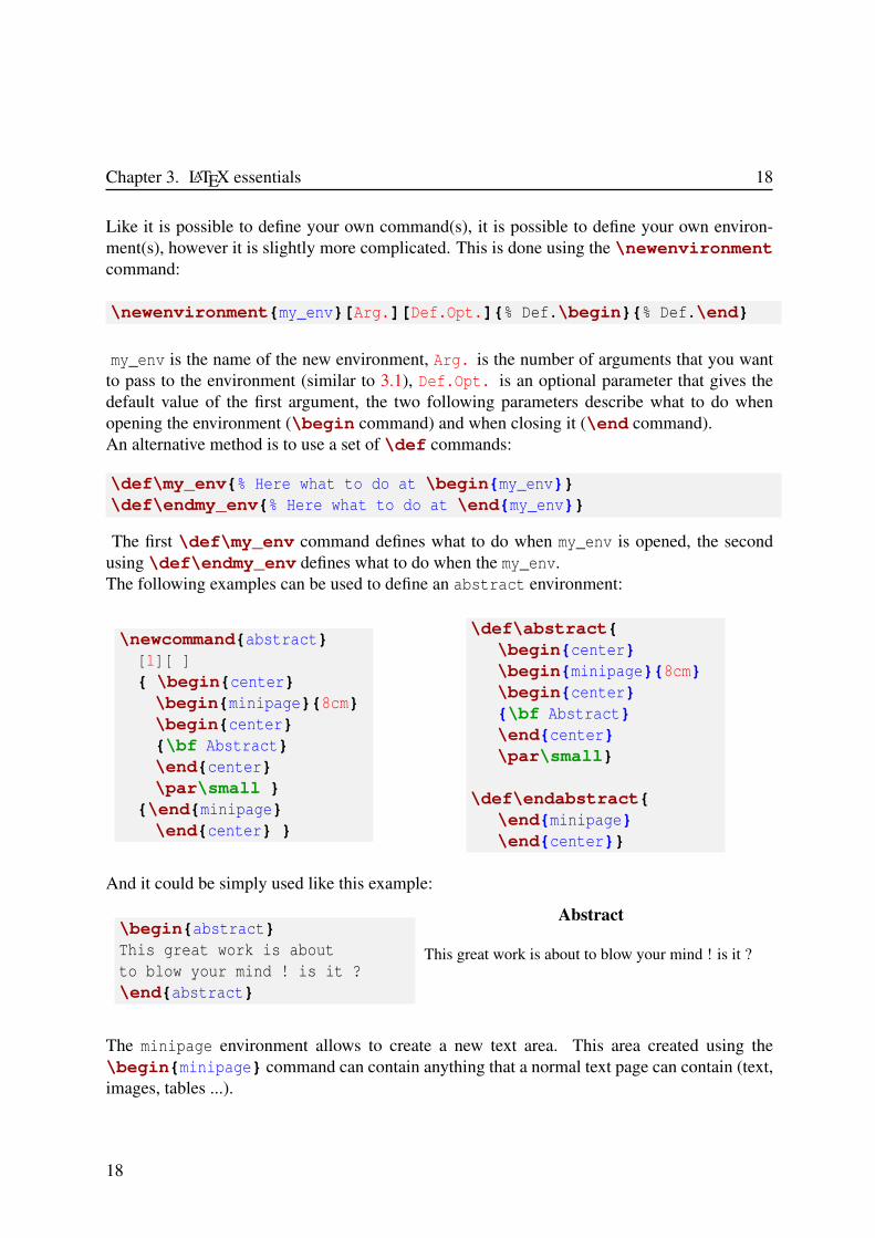
Like it is possible to define your own command(s), it is possible to define your own environ-ment(s), however it is slightly more complicated. This is done using the \newenvironmentcommand:

\newenvironment{my_env}[Arg.][Def.Opt.]{% Def.\begin}{% Def.\end}

my_env is the name of the new environment, Arg. is the number of arguments that you wantto pass to the environment (similar to 3.1), Def.Opt. is an optional parameter that gives thedefault value of the first argument, the two following parameters describe what to do whenopening the environment (\begin command) and when closing it (\end command).An alternative method is to use a set of \def commands:

\def\my_env{% Here what to do at \begin{my_env}}

\def\endmy_env{% Here what to do at \end{my_env}}

The first \def\my_env command defines what to do when my_env is opened, the secondusing \def\endmy_env defines what to do when the my_env.The following examples can be used to define an abstract environment:

\newcommand{abstract}

[1][ ]

{ \begin{center}

\begin{minipage}{8cm}

\begin{center}

{\bf Abstract}

\end{center}

\par\small }

{\end{minipage}

\end{center} }

\def\abstract{

\begin{center}

\begin{minipage}{8cm}

\begin{center}

{\bf Abstract}

\end{center}

\par\small}

\def\endabstract{

\end{minipage}

\end{center}}

And it could be simply used like this example:

\begin{abstract}

This great work is about

to blow your mind ! is it ?

\end{abstract}

Abstract

This great work is about to blow your mind ! is it ?

The minipage environment allows to create a new text area. This area created using the\begin{minipage} command can contain anything that a normal text page can contain (text,images, tables ...).

18

19 3.3. Packages

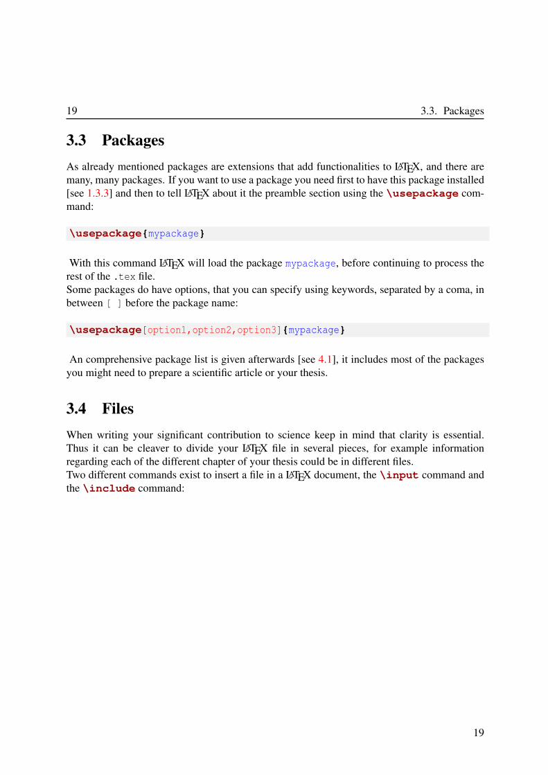
3.3 Packages

As already mentioned packages are extensions that add functionalities to LATEX, and there aremany, many packages. If you want to use a package you need first to have this package installed[see 1.3.3] and then to tell LATEX about it the preamble section using the \usepackage com-mand:

\usepackage{mypackage}

With this command LATEX will load the package mypackage, before continuing to process therest of the .tex file.Some packages do have options, that you can specify using keywords, separated by a coma, inbetween [ ] before the package name:

\usepackage[option1,option2,option3]{mypackage}

An comprehensive package list is given afterwards [see 4.1], it includes most of the packagesyou might need to prepare a scientific article or your thesis.

3.4 Files

When writing your significant contribution to science keep in mind that clarity is essential.Thus it can be cleaver to divide your LATEX file in several pieces, for example informationregarding each of the different chapter of your thesis could be in different files.Two different commands exist to insert a file in a LATEX document, the \input command andthe \include command:

19


\documentclass{book}

% Preamble section

\input{preamble}

\includeonly{intro,chapter1}

\begin{document}

% Main body section

\include{intro}

\include{chapter1}

\include{chapter2}

\include{conclu}

\end{document}

=⇒ reading the file: preamble.tex

=⇒ reading the file: intro.tex

=⇒ reading the file: chapter1.tex

=⇒ reading the file: chapter2.tex

=⇒ reading the file: conclu.tex

LATEX automatically adds the .tex extension to the file names given by the \input and\include commands.Therefor in this example LATEX will look for the file preamble.tex in the preamble section,this file can contains \usepackage, commands and environments declaration(s).Afterwards in the main body section, LATEX will read the files intro.tex, chapter1.tex,chapter2.tex and conclu.tex containing different the parts of the manuscript.Only the main .tex file contains the \documentclass, \begin{document}, and\end{document} commands. The contents of the file which name is specified by the\input or the \include commands is simply inserted at the location of the commandduring the compilation process.The \include command inserts the file in the document using a new page, while the \inputcommand inserts the file without condition.Also the \include command can be activated or deactivated by the \includeonly com-mand. Therefore in the previous example only the files into.tex and chapter1.tex will beinserted in the main document during the compilation. The combination of \include the\includeonly command can be very useful when preparing large documents with extendedchapters like your thesis.

20

My first LATEX document

4.1 Preparing the preamble

Before starting to write your manuscript you need to ensure that all packages and commandsthat this work might requires are listed in the preamble of the main LATEX file. You can defineyour own commands here [see 3.1], remember that doing so can considerably help to simplythe writing of the manuscript. Finally you can ask latex to read file(s) to get extra information.An interesting example of the preamble section of your main LATEX file is the following:

\documentclass{article}

\input{preamble}

\begin{document}

Here the preamble section consists of a single command, that tells LATEX to read a file, this filecalled preamble.tex contains all the information regarding the packages and commands. Oneof the advantages of this method is to have a main file easier to read, since it now only containsyour precious manuscript. Also if you decide to keep working using LATEX you could recall thesame preamble.tex file.

A comprehensive example of the preamble section is given afterwards, and most of thepackages you might need to write your piece of science and print your mark in history are listedhereafter, you just need to adapt it to your personal use:

21

Chapter 4. My first LATEX document 22

% To have an input font encoding that support special characters

\usepackage[utf8]{inputenc}

% To have an output font encoding that support special characters

\usepackage[T1]{fontenc}

% To define the language of the document

\usepackage[english]{babel}

% Much better font for the PDF file

\usepackage{pslatex}

% Hyperlinks for the PDF file

\usepackage[pdfauthor = {Sébastien Le Roux},

pdftitle = {LaTeX tutorial},

pdfsubject = {LaTeX tutorial},

pdfkeywords = {LaTeX Users Manual Guide Basics Help},

pdfcreator = {LaTeX+DviPDF},

pdfproducer = {LaTeX+DviPDF},

pdfstartview = FitV, % Adjust the document to the window at startup

dvips = true, % Use hyperref with dvips

colorlinks = true, % Colored hypertext links

plainpages = false, % Do page number anchors as plain arabic

pagebackref = true, % Allows to add links in the bibliography ...

backref = page, % .. that points toward the appropriate pages

hyperindex = true, % Add hypertext links in the appendix

linktocpage = true, % Links on the page numbers and not the text

breaklinks = true, % To write the long hyperlinks on more than one line

urlcolor = blue, % Color for external hyperlinks

linkcolor = red, % Color for internal hyperlinks

bookmarks = true, % To create the section marks pour Acrobat Reader

bookmarksopen = false % Is the document tree entirely opened at startup

]{hyperref}

% Insert images

\usepackage{graphicx}

% Colors

\usepackage{xcolor}

% Enumerations

\usepackage{enumerate}

% Mathematics

\usepackage{amsmath}

\usepackage{amssymb}

\usepackage{amscd}

\usepackage{theorem}

% Tables

\usepackage{hhline}

\usepackage{multirow}

\usepackage{tabls}

% To use landscape pages in a portrait document

\usepackage{lscape}

% Spaces between lines

\usepackage{setspace}

%\onehalfspacing

%\doublespacing

%\setstretch{3}

22

23 4.2. Writing the manuscript

4.2 Writing the manuscript

From now on every command, environment, text is going to be written in the main body of thedocument, thus after the line \begin{document}.

4.2.1 Writing text

4.2.1.1 Special characters

You are now ready to prepare your first manuscript, before starting you need to know that LATEXconsiders some particular characters as commands. If you do not want LATEX to shout at youduring the compilation process [see. 9] you should be familiar with these 10 characters:

\ # % ∼ { } $ _ ˆ

• \ is the beginning of a command - [see 3.1]

• # is used when creating commands - [see 3.1]

• % starts a comments, everything that follow on the same line is not interpreted, read orcompiled by LATEX

• ∼ creates a non-breaking space

• { and } highlight the beginning and the end of a command or an environment

• $, _ and ˆ - [see 4.2.4]

• & - [see 4.2.5]

23


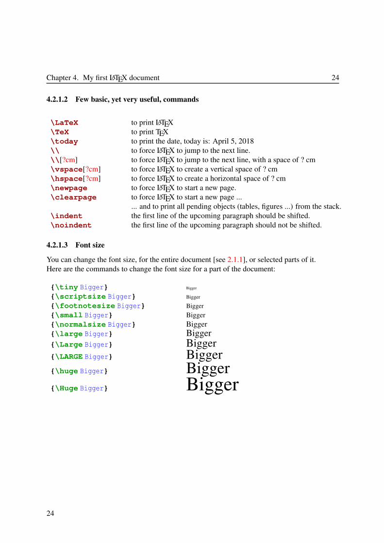
4.2.1.2 Few basic, yet very useful, commands

\LaTeX to print LATEX\TeX to print TEX\today to print the date, today is: April 5, 2018\\ to force LATEX to jump to the next line.\\[?cm] to force LATEX to jump to the next line, with a space of ? cm\vspace[?cm] to force LATEX to create a vertical space of ? cm\hspace[?cm] to force LATEX to create a horizontal space of ? cm\newpage to force LATEX to start a new page.\clearpage to force LATEX to start a new page ...

... and to print all pending objects (tables, figures ...) from the stack.\indent the first line of the upcoming paragraph should be shifted.\noindent the first line of the upcoming paragraph should not be shifted.

4.2.1.3 Font size

You can change the font size, for the entire document [see 2.1.1], or selected parts of it.Here are the commands to change the font size for a part of the document:

{\tiny Bigger} Bigger

{\scriptsize Bigger} Bigger

{\footnotesize Bigger} Bigger

{\small Bigger} Bigger{\normalsize Bigger} Bigger{\large Bigger} Bigger{\Large Bigger} Bigger{\LARGE Bigger} Bigger{\huge Bigger} Bigger{\Huge Bigger} Bigger

24


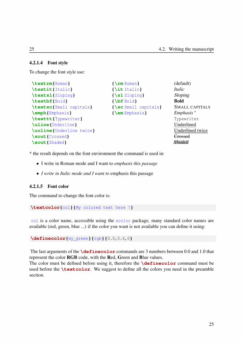
4.2.1.4 Font style

To change the font style use:

\textrm{Roman} {\rm Roman} (default)\textit{Italic} {\it Italic} Italic

\textsl{Sloping} {\sl Sloping} Sloping\textbf{Bold} {\bf Bold} Bold

\textsc{Small capitals} {\sc Small capitals} SMALL CAPITALS

\emph{Emphasis} {\em Emphasis} Emphasis ∗

\texttt{Typewriter} Typewriter

\uline{Underline} Underlined\uuline{Underline twice} Underlined twice\sout{Crossed} Crossed\xout{Shaded} /////////Shaded

* the result depends on the font environment the command is used in:

• I write in Roman mode and I want to emphasis this passage

• I write in Italic mode and I want to emphasis this passage

4.2.1.5 Font color

The command to change the font color is:

\textcolor{col}{My colored text here !}

col is a color name, accessible using the xcolor package, many standard color names areavailable (red, green, blue ...) if the color you want is not available you can define it using:

\definecolor{my_green}{rgb}{0.0,0.6,0}

The last arguments of the \definecolor commands are 3 numbers between 0.0 and 1.0 thatrepresent the color RGB code, with the Red, Green and Blue values.The color must be defined before using it, therefore the \definecolor command must beused before the \textcolor. We suggest to define all the colors you need in the preamblesection.

25


4.2.2 Title, authoring and abstract

It can be useful to inform your reader about what they are going to read, depending on thedocument class (book, article, revtex4-1, achemso ...) the instructions can change slightlyfor details give a look to the help pages of the corresponding class. This example can be usedfor most document classes:

% Give the title of your thesis / article

\title{My revolutionary science project}

% Name the authors

\author{M. Me, Y. You and H. He}

% You can even provide an abstract

\begin{abstract}

This great work is about to blow your mind !

\end{abstract}

% Now create the title page using all of the above

\maketitle

Detail examples for each editor related document classes are provided in [Chap. 7].

4.2.3 Organizing your document

If you want people to read and understand your work, it is important to organize it prop-erly. That means divide it in parts, chapters, sections or other pieces that help to clarify itscontent for the reader. All these commands (see Tab. 4.1) have a similar structure and usage,hereafter we will use the \section as an example of any of the commands in table [Tab. 4.1].

\section[Section shortname]{Section title}

The first option of the command, the [ ], is not mandatory and can be used to modify the nameof the section that will appear in the Table Of Contents, TOC, if any. The default name of thesection in the TOC is given by the second option of the command, its real title in the document.

\section{My great section}

\subsection{My great subsection}

=⇒1 My great section

1.1 My great subsection

26


Table 4.1 LATEX commands to organize your document.

Command Document class

\part

\chapter

\section

\subsection

\subsubsection

\paragraph

\subparagraph

=⇒

book, article∗

book

book, article∗

book, article∗

book, article∗

book, article∗

book, article∗

* Including the revtex4-1, iopart, elsarticle and achemso classes.

27


The numbering of the chapters, parts, sections, etc, will be done automatically by LATEX, thusthere is no need for the user to specify any number.If you do not want the section to be numbered use a * symbol:

\section*{My great section}

\subsection*{My great subsection}

=⇒My great section

My great subsection

Note that the section(s) will still appears in the TOC, but without number(s).One more command that you might need to organize your document is \appendix that indi-cates the end of the main part of the manuscript and the start of the appendix. In the appendixyou use all the commands presented in table [Tab. 4.1] however the numbering will not be donewith numbers anymore but with letters:

\chapter{My final chapter}

% Final chapter body

\section{My first section}

% First section body

\section{My second section}

% Second section body

\chapter*{Conclusion}

% The conclusion

\appendix

\chapter{Additional data}

=⇒

Chapter 5My final chapter

1 My first section

2 My second section

Conclusion

Appendix AAdditional data

In some classes, like book, it is possible to create a TOC, a list of figures and a list of tables:

% Create the table of content

\tableofcontent

% Add a list of figures (= list of all \begin{figure} and caption)

\listoffigures

% And a list of tables (= list of all \begin{table} and caption)

\listoftables

28


4.2.4 Inserting a math equation

They are two main possibilities to insert a math equation, or to use what is called the mathemat-ics mode:

• the standard, in-line, math mode: $Math expression here$

• the equation math mode: \begin{equation}Math expression here\end{equation}

The math modes present specific properties:

• Text letters (a,A → z,Z) are written in italic (a,A → z,Z), however numbers, symbols andpunctuation signs are written in standard roman characters.

• Superscript writing using the ˆ character and subscript writing using the _ character:

$6.022\times10^{23}$ \\

CH$_3$CH$_2$OH \\

NH$_3^+$

=⇒6.022×1023

CH3CH2OHNH+

3

Note that if no brackets, { }, are used, then only the first letter/symbol/number followingthe ˆ and the _ characters will be affected and upper-lower-scripted.

• Many, many, many symbols are accessible using commands, such as:

− Greek letters: \alpha \beta \gamma \Gamma \delta \Delta

α β γ Γ δ ∆

− Math operators: \sum \prod \frac{1}{2} \sqrt[x]{y} \int

∑ ∏ 12

x√

y∫

− Math accents: \vec{v} \dot{a} \bar{h} \widehat{abc}

~v a h abc

− Symbols: \hbar \infty \times \div \pm

~ ∞ × ÷ ±

29


Using the first method, using $ $ symbols, also called ’in-line’ equation it is possible to insertmaths in the text, for example the instructions:

$\sum_{i=1}^{N} \frac{x-1}{\sqrt{\delta}} = \infty$

will be rendered like this in a text line, ∑Ni=1

x−1√δ= ∞, allowing to continue the discussion.

The other method using an equation environment adds a number to your equation, sothat you can refer to this equation somewhere else in the document [see 4.2.8]:

\begin{equation}

\sum_{i=1}^{N} \frac{x-1}{\sqrt{\delta}} = \infty

\end{equation}

It will also be rendered separately from the text:

N

∑i=1

x−1√δ

= ∞ (4.1)

For other examples [see 7].

4.2.5 Inserting a table

To create a table it is required to use the table and the tabular environments, the first allowsto insert a caption and make reference(s) to this table elsewhere in the document [see 4.2.8],while the second allows to organize elements in columns and rows:

\begin{table}

\begin{tabular}{l|cr||}

& $\alpha$ & $\beta$ \\

\hline

\hline

a & 2.0 & $1\times10^{-4}$ \\

b & -3.0 & $\sqrt5$ \\

c & 1.0 & $1\times10^2$ \\

\hline

\end{tabular}

\caption{My interesting table}

\end{table}

α β

a 2.0 1×10−4

b −3.0√

5c 1.0 1×102

Table 4.2 My interesting table

30


The options of the \begin{tabular} command define the shape of the table, in the previousexample: {l|cr||}. The number of column(s) in the table is given by the number of letters,here 3 letters hence the table will have 3 columns. The letter itself defines how the text iscentered in the corresponding column: l=left, c=center or r=right. The pipe symbol, {|} isused to draw separator(s) (by default straight lines) between columns.In the table it-self, the \hline is used to draw separator(s) between rows. On the same row,columns are separated using the & symbol, the line is terminated using the \\ symbol.

In a multicolumn document it is possible to use the \begin{table*} and \end{table*}

commands to produce a table that use the entire width of the page instead of the default widthof a single column.


4.2.6 Inserting an image

To insert an image it is required to use the figure environment, to insert a caption and make ref-erence(s) to this figure elsewhere in the document [see 4.2.8], and the \includegraphicscommand provided by \usepackage{graphicx} added to the preamble section [see 4.1].The graphicx package allows to import and use most type of images, however it is strongly

recommended to use PostScript, .ps, or preferably Encapsulated PostScript, .eps, images withLATEX.

\begin{figure}

\includegraphics{image.eps}

\caption{My interesting figure}

\end{figure}

Figure 4.1 My interesting figure

31


The \includegraphics command accepts many optional keywords like:

• keepaspectratio=true % or false

• scale=0.75

• width=5cm

• height=8cm

• angle=90

• draft=false, this is the default value, if you set this option on true the image is notinserted, instead you will see a blank space of the same size, this could be very usefulwhen preparing a large manuscript with many images, like your thesis.

• natwidth=640, used to solve bounding box errors [see 9]

• natheight=480, used to solve bounding box errors [see 9]

\includegraphics[width=10cm,keepaspectratio=true,draft=true]{image.eps}

In a multicolumn document it is possible to use the \begin{figure*} and \end{figure*}commands to produce a figure that uses the entire width of the page instead of the default widthof a single column.


32


4.2.7 Inserting a list / enumeration

You can insert a list using the itemize environment and the \item command:

\begin{itemize}

\item Element 1

\item Element 2

\begin{itemize}

\item Element 3

\item Element 4

\begin{itemize}

\item Element 5

\item Element 6

\end{itemize}

\end{itemize}

\item Element 7

\end{itemize}

=⇒

• Element 1

• Element 2

– Element 3

– Element 4

∗ Element 5

∗ Element 6

• Element 7

For an enumeration use the enumerate environment and the \item command:

\begin{enumerate}

\item Element 1

\item Element 2

\begin{enumerate}

\item Element 3

\item Element 4

\begin{enumerate}

\item Element 5

\item Element 6

\end{enumerate}

\end{enumerate}

\item Element 7

\end{enumerate}

=⇒

1. Element 1

2. Element 2

(a) Element 3

(b) Element 4

i. Element 5

ii. Element 6

3. Element 7

33


4.2.8 Inserting a reference

To make a reference to an element can be achieved using the two commands \label and\ref. The first one is used to create a keyword associated with an object, the second one isused to make reference to this keyword and therefore to the object it-self:

\section{My third section}

\label{sec-3}

I like what’s in figure \ref{pinte}

\section{My fourth section}

\begin{figure}

\includegraphics{image.eps}

\caption{\label{pinte}My interesting figure}

\end{figure}

As already said in section \ref{sec-3}

I like what’s in figure \ref{pinte}

3 My third section

I like what’s in figure 4.2

4 My fourth section

Figure 4.2 My interesting figure

As already said in section 3

I like what’s in figure 4.2

There is no need to number anything, LATEX does it for you. You can add a label using the\label command to pretty much any object in the document, including all the objects andenvironments presented previously in this HowTo. There is only one simple rule to respect forthe floating objects, like the tables or the figures, and that is to put the \label command insidethe \caption command. Finally remember that each label, in other word each KEYWORD, usedin the \label{KEYWORD} command, must be unique.

34


4.2.9 Inserting web links and emails

To insert an hypertext link or an email address use the \href command. The \href commandtakes 2 arguments, the first one is the web link or the email address, the second is the text to bedisplayed in the final document, ex:

Link:\href{https://www.latex-project.org/}{The \LaTeX\ project web page}

Mail:\href{mailto:[email protected]}{Sébastien Le Roux}

Will be be rendered as:Link:The LATEX project web pageMail:Sébastien Le Roux

4.2.10 Inserting a bibliography

There are 2 methods to create references and the corresponding bibliography in your TEXdocument, both require references to be inserted using the \cite command:

The work in this article is good, really good,

it is even better than some previous work in Ref.\cite{old_work_a},

it will clearly be more cited that Ref.\cite{old_work_b}

To the keyword used in the \cite command corresponds an entry in the bibliography that youneed to create. You have 2 methods to achieve this goal:

1. Use the thebibliography environment, and create an entry for the reference using the\bibitem command:

\begin{thebibliography}

\bibitem{old_work_a}

D. umb and I. diot,

J. Non-Smart. Sci. \textbf{00}, 0000-0007 (2015).

\bibitem{old_work_b}

R. Car and M. Parrinello,

Phys. Rev. Lett. \textbf{55}, 2471-2474 (1985).

\end{thebibliography}

You need to create all the entries in the bibliography your-self, eventhough it is notcomplicated it has to be done very carefully. You define the style of the citations yourselfusing LATEX commands, ie. the author name format, the order the authors list, journal,year, appear in ... Be careful to create the entries in the order you want them to appear inthe bibliography section. To have the citations in the order they appear in the article/thesiscan be tricky, in particular in you keep modifying the source file.

35


mailto:[email protected]


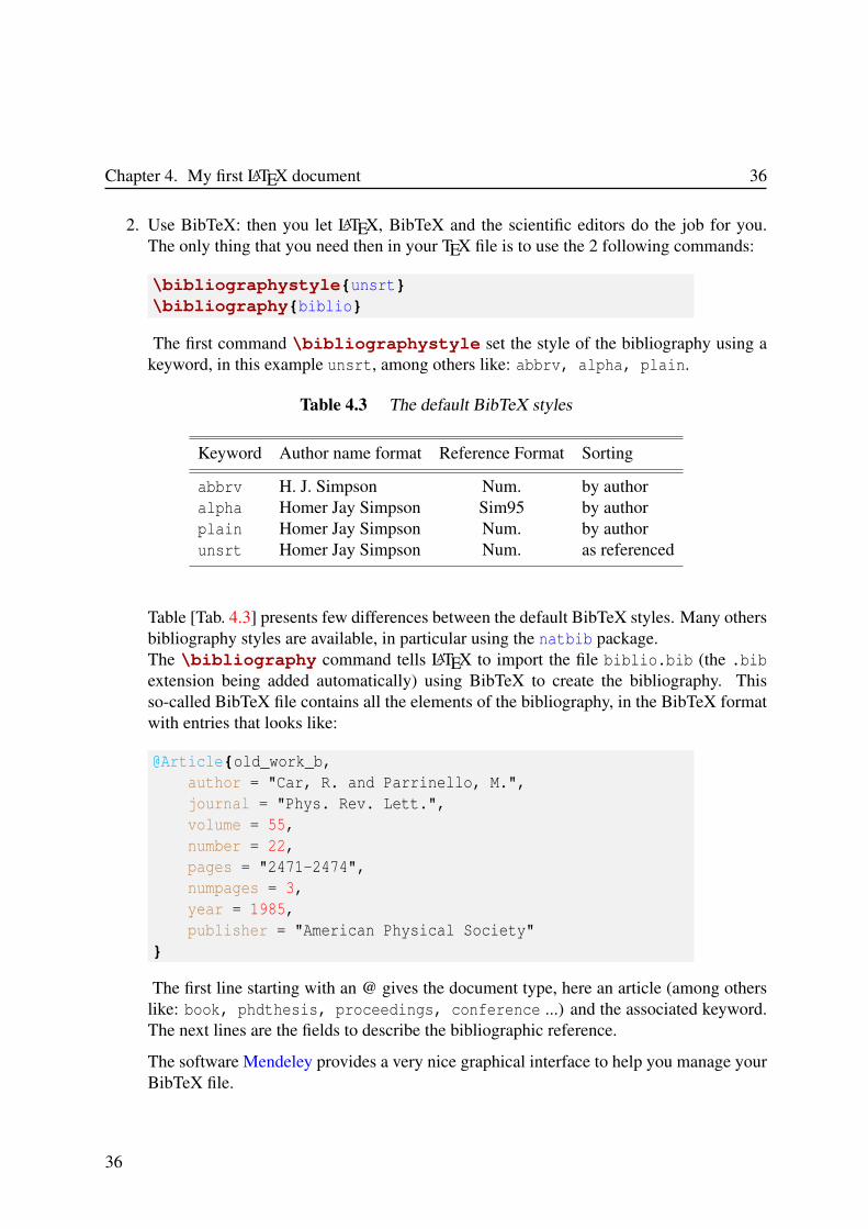
2. Use BibTeX: then you let LATEX, BibTeX and the scientific editors do the job for you.The only thing that you need then in your TEX file is to use the 2 following commands:

\bibliographystyle{unsrt}

\bibliography{biblio}

The first command \bibliographystyle set the style of the bibliography using akeyword, in this example unsrt, among others like: abbrv, alpha, plain.

Table 4.3 The default BibTeX styles

Keyword Author name format Reference Format Sorting

abbrv H. J. Simpson Num. by authoralpha Homer Jay Simpson Sim95 by authorplain Homer Jay Simpson Num. by authorunsrt Homer Jay Simpson Num. as referenced

Table [Tab. 4.3] presents few differences between the default BibTeX styles. Many othersbibliography styles are available, in particular using the natbib package.The \bibliography command tells LATEX to import the file biblio.bib (the .bib

extension being added automatically) using BibTeX to create the bibliography. Thisso-called BibTeX file contains all the elements of the bibliography, in the BibTeX formatwith entries that looks like:

@Article{old_work_b,

author = "Car, R. and Parrinello, M.",

journal = "Phys. Rev. Lett.",

volume = 55,

number = 22,

pages = "2471-2474",

numpages = 3,

year = 1985,

publisher = "American Physical Society"

}

The first line starting with an @ gives the document type, here an article (among otherslike: book, phdthesis, proceedings, conference ...) and the associated keyword.The next lines are the fields to describe the bibliographic reference.

The software Mendeley provides a very nice graphical interface to help you manage yourBibTeX file.

36

https://www.mendeley.com


Why is BibTeX so great:

• Most of the scientific editors provide the BibTeX entries for their publications,which means that you only need to browse their web sites, find the page of theappropriate article, and copy-paste the entry in your own BibTeX file, then simplyuse the corresponding keyword in your manuscript.

• You can use the same BibTeX file for all your works with LATEX, this means that youjust need to do prepare an entry the first time you need the reference, then simplyrecall the appropriate keyword.

• No matter the number of entries in the BibTeX file LATEX and BibTeX will only usethe ones cited in your article and ignore the others.

• No need to take care of the order of the entries in the BibTeX file, the citations inyour bibliography will be sorted automatically.

37


To use BibTeX the compilation sequence changes, and you need to enter the followingsequence of commands:


...

user@localhost ~]$ bibtex manuscript

...


...


...

In Texmaker you need to change the "Quick Build" options to "LaTeX + Bib(la)Tex +LaTeX (x2) + dvips + ps2pdf + See PDF", see figure [Fig. 4.3].

Figure 4.3 The "Quick Build" tab in the Texmaker options dialog box for BibTeX. At thispoint you need to select the "LaTeX + Bib(la)Tex + LaTeX (x2) + dvips + ps2pdf+ See PDF" option.

38

Spell checking

5.1 Using the command line

You can check the spelling of your LATEX manuscript using the aspell command:

user@localhost ~]$ aspell -c -t --lang=en_EN manuscript.tex

The options are:

• -c : to check spelling.

• -t : the document to check is a TEX file, all TEX and LATEX commands will be ignored.

• -lang=en_EN : the language of the document (in this case English), among the dictionar-ies installed on your OS. For Linux and MacOS available dictionaries are listed in:

– /usr/share/myspell/

– /usr/share/locale/

Following this command you will enter an interactive mode to check the content of your TEXfile, simply follow the instructions to correct it if necessary.

You could also used a BASH script, thus providing that the following script, named check, isinstalled somewhere in your PATH (see [2] for details):

#!/bin/bash

TFILE=$1

aspell -c -t --lang=en_EN $TFILE".tex"

You could spell check your LATEX document simply using:

user@localhost ~]$ check manuscript

39

Chapter 5. Spell checking 40

5.2 Using Texmaker

1. Open the "Options → Configure Texmaker" dialog:

Figure 5.1 Open the "Configure Texmaker" dialog box.

2. Browse the "Editor" ("Editeur" in French) tab, and check that the appropriate dictio-nary is being used:

Figure 5.2 The "Editor" tab in the Texmaker options dialog box. At this point you need toselect the appropriate dictionary.

40

41 5.2. Using Texmaker

3. Use "Check Spelling" button in the file menu (or the Ctrl+Maj+F7 keyboard shortcut) tocheck your manuscript:

Figure 5.3 Spell checking in Texmaker.

For Windows dictionnaries are installed with Texmaker and can be found in:

• C:\Program Files (x86)\Texmaker\

41

LATEX advantages and drawbacks

Drawbacks

You will need to learn few things about programming

It is obvious that the first thing about LATEX is that you need to learn a bit, to say the least, aboutprogramming. If your are not willing to spend some time learning how things are behind thecurtains, well forget about LATEX.

You will need to be patient

• Because you will not see immediately the result of your work.Most people spend a lot of time going back and forth between the source file and thePDF file. That is the wrong way to work with LATEX (and that is what you will start todo anyway): as soon as you inserted a few lines, or commands, you want to know how itlooks like, and you build the PDF file.That works for small documents, forget about it for real ones, like your thesis or an article,in particular if you insert graphics, and you will. The more images you include, the longerit takes to build the PDF file, think about it when you will prepare your thesis (and alsothink about the draft option for the \includegraphics command).

• Because you will waste time trying to find that f*****g command your are looking for.That is the way it is, I wish I could tell you that you will be fluent in LATEX by the end ofthe day, and the commands will come to you naturally. Nope. As everybody, and evenafter years of experience, you will still waste time to look for a particular command to dothat particular thing you really need to do.

• Because when you will find that f*****g command it will not work.And you will need to take time to install the package that contains this precious commandthat you really really need.

• Because the compilation will fail, many times - see bellow.

43

Chapter 6. LATEX advantages and drawbacks 44

You will need to be organized

As you are a scientist, or about to become one, this should not be too much of a problem.Why is it so important to be well organized:

• To avoid to waste too much time debugging errors during the compilation process.The compilation will fail, many times, because of silly mistakes like:

– Forget to use an \end command to close a \begin command.

– To miss or have an extra symbol: {, [, (

– To miss or have an extra symbol: }, ], )

– To miss or have an extra symbol: $

– To miss or have an extra symbol: &

Trying to find where the error comes from, will be time consuming, and as much aspossible you want to avoid that.

• To keep your working directory clean enough to know what is going on.Indeed after the compilation process of your main *.tex file the directory will be filledwith many files, created by LATEX and potentially BibTeX. It will also contains images,probably a significant number for your thesis. Think about creating sub-directory(ies) tosort and organize everything, it will be easier to find the information you might look forafterwards.

Advantages

If you are not too scared already, then hope for you there is young Padawan.Your ally is the force in LATEX and a powerful ally it is !Now is the time to learn why the light side of the force is the way to go.

May the force in LATEX be with you !

It looks great !

You will see by yourself soon enough that there is no way to match the quality of a documentproduced using LATEX.

No more journal layout problems !

You just need to use the proper keyword, or option, usually in the \documentclass, some-times in the preamble section, to have the job perfectly done by LATEX.

44

45

Cross-referencing and bibliography made easy !

No numbering to be done, simply use a different keyword for each object and LATEX takes careof the rest: numbering, hypertext links, etc.Using BibTeX you only have to do the job once, the first time that you add an entry in the *.bibfile. After that simply re-use the appropriate keyword to cite the corresponding publication. Thismeans that this BibTeX file can be shared between all your LATEX projects.

You will save time, a lot !

Yes you will. Think about the time you would need with a WYSIWYG editor to:

• Prepare the layout of the document

• Organize properly the document

• Organize the cross referencing

• Organize the bibliography

Hopefully by now you understand that with LATEX this can become almost automatic. Conse-quently you can save a lot of time to do something else.

45

Examples

7.1 Title and authors

7.1.1 RevTex 4.1 - "revtex4-1"

\documentclass[prb,twocolumn,superscriptaddress]{revtex4-1}

% Use the "superscriptaddress" in the documentclass options.

\begin{document}

\title{My amazing work !}

\author{M. Me}

\affiliation{My great institution - France}

\author{Y. You}


\author{H. He}

\affiliation{The third author institution - USA}

\begin{abstract}


\end{abstract}

\maketitle

% At this point the article start

\end{document}

47

Chapter 7. Examples 48

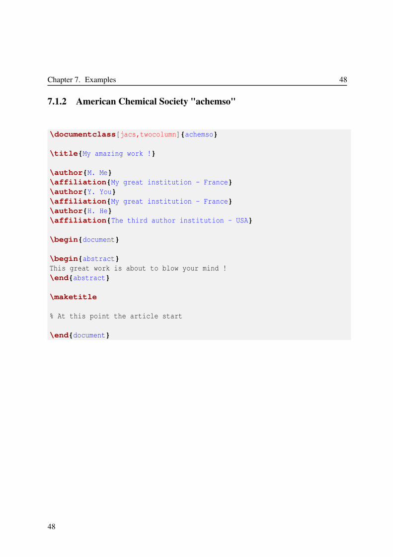
7.1.2 American Chemical Society "achemso"

\documentclass[jacs,twocolumn]{achemso}


\author{M. Me}


\author{Y. You}


\author{H. He}

\affiliation{The third author institution - USA}

\begin{document}

\begin{abstract}


\end{abstract}

\maketitle


\end{document}

48

49 7.1. Title and authors

7.1.3 Elsevier "elsarticle"

\documentclass[jncs,twocolumn]{elsarticle}

\begin{document}


\author[1]{M. Me}

\author[1]{Y. You}

\author[2]{H. He}

\address[1]{My great institution - France}

\address[2]{The third author institution - USA}

\begin{abstract}


\end{abstract}

\maketitle


\end{document}

49


7.1.4 Institute Of Physics "iopart"

\documentclass[jpcm,twocolumn]{iopart}

\begin{document}


\author{M. Me$^1$}

\author{Y. You$^1$}

\author{H. He$^2$}

\address{(1) My great institution - France}

\address{(2) The third author institution - USA}

\begin{abstract}


\end{abstract}

\maketitle


\end{document}

50

51 7.2. Tables and figures

7.2 Tables and figures

\begin{table}[!h]

\caption{Label and description of the e- acceptor diimide cores studied.}

\vspace{0.3cm}

\begin{tabular}{rlcllc}

Id & Label & $N$ & Formula & \multicolumn{2}{c}{Diimide familly + 3D} \\

\hline

\\

& & & & & \multirow{4}{5cm}

{\includegraphics[width=0.9\linewidth,keepaspectratio=true,draft=false]

{img/NDI.eps}} \\

1 & NDI & 32 & C$_16$H$_10$O$_4$N$_2$ &

\multirow{2}{4cm}{\bigg}Naphthalene} \\

2 & NDI\_F4 & 38 & C$_{16}$H$_6$O$_4$N$_2$F$_4$ \\

\\

\\

3 & ADI & 38 & C$_20$H$_12$O$_4$N$_2$ &

\multirow{4}{4cm}{\Bigg}Anthracene} \\

\multirow{4}{5cm}

{\includegraphics[width=1.0\linewidth,keepaspectratio=true,draft=true]

{img/ADI.eps}} \\

4 & ADI\_F2 & 38 & C$_{20}$H$_{10}$O$_4$N$_2$F$_2$ \\

5 & ADI\_CN2 & 40 & C$_{22}$H$_{10}$O$_4$N$_4$ \\

6 & ADI\_Br2 & 38 & C$_{20}$H$_{10}$O$_4$N$_2$Br$_2$ \\

\end{tabular}

\end{table}

The table above provides and example of the usage for the following commands:

• \multicolumn

usage: \multicolumn{#NUM}{#LAYOUT}{Data to display}}with: #NUM= number of column, #LAYOUT = l=left, c=center, r=right

• \multirow (requires the multirow package)

usage: \multirow{#NUM}{#WIDTH}{Data to display}}with: #NUM= number of row, #WIDTH = width of the text

• \includegraphics, comparison of the options draft=false and draft=true

51


Table 7.1 Label and description of the e- acceptor diimide cores studied.

Id Label N Formula Diimide familly + 3D

1 NDI 32 C16H10O4N2}

Naphthalene2 NDI_F4 38 C16H6O4N2F4

5 ADI 38 C20H12O4N2 }Anthracene

img/ADI.eps

6 ADI_F2 38 C20H10O4N2F27 ADI_CN2 40 C22H10O4N48 ADI_Br2 38 C20H10O4N2Br2

52

53 7.3. Equations

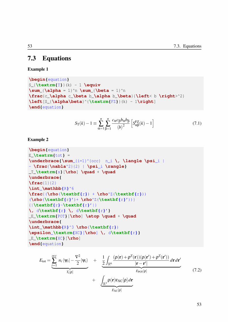
7.3 Equations

Example 1

\begin{equation}

S_{\textrm{T}}(k) - 1 \equiv

\sum_{\alpha = 1}^n \sum_{\beta = 1}^n

\frac{c_\alpha c_\beta b_\alpha b_\beta}{\left< b \right>^2}

\left[S_{\alpha\beta}^{\textrm{FZ}}(k) - 1\right]

\end{equation}

ST(k)−1 ≡n

∑α=1

n

∑β=1

cαcβbαbβ

〈b〉2

[SFZ

αβ(k)−1]

(7.1)

Example 2

\begin{equation}

E_\textrm{tot} =

\underbrace{\sum_{i=1}^{occ} n_i \, \langle \psi_i |

- \frac{\nabla^2}{2} | \psi_i \rangle}

_T_\textrm{s}[\rho] \quad + \quad

\underbrace{

\frac{1}{2}

\int_\mathbb{R}^6

\frac{(\rho(\textbf{r}) + \rho^Z(\textbf{r}))

(\rho(\textbf{r}’)+ \rho^Z(\textbf{r}’))}

{|\textbf{r}-\textbf{r}’|}

\, d\textbf{r} \, d\textbf{r}’}

_E_\textrm{POT}[\rho] \atop \quad + \quad

\underbrace{

\int_\mathbb{R}^3 \rho(\textbf{r})

\epsilon_\textrm{XC}[\rho] \, d\textbf{r}}

_E_\textrm{XC}[\rho]

\end{equation}

Etot =occ

∑i=1

ni 〈ψi|−∇2

2|ψi〉

︸︷︷︸Ts[ρ]

+12

∫R6

(ρ(r)+ρZ(r))(ρ(r′)+ρZ(r′))|r− r′| drdr′

︸︷︷︸EPOT[ρ]

+∫R3

ρ(r)εXC[ρ]dr︸︷︷︸

EXC[ρ]

(7.2)

53

Partial glossary

8.1 Useful commands

8.1.1 In text mode

• \aa

- The angström symbol: å

• \AA

- The Angström symbol: Å

• \footnote{Here is my footnote}

- To produce footnote(s):

I want to insert\footnote{a footnote here}.

I want to insert1.

• \par

- To start a new paragraph.

• \caption

- To insert a caption: \caption[Small caption]{Full caption}

The first optional argument is the name of the object for the list of figures or the list oftables, this is interesting if the caption of the figure or the table is long.

1a footnote here

55

Chapter 8. Partial glossary 56

8.1.2 In math mode

• \bullet

- the symbol: •

• \rangle

- the symbol: 〉

• \langle

- the symbol: 〈

• \underbrace{Equation}_{Information}

To underbrace part(s) of an equation:

\underbrace{y = a×x + b}_\textrm{Too simple !} y = a× x+b︸︷︷︸Too simple !

see equation 7.2 for more examples.

• \lbrack

- the symbol: [

• \rbrack

- the symbol: ]

• \left + symbol in: {,(,[ .. and \right + symbol in: },),] ...

ensure that the symbols to be displayed immediately after the commands \left and\right will be large enough compared to the expression between \left and \right,see equation 7.1 for an example.

• \sum_{From}ˆ{To}

The sum symbol:

\sum_{i=0}ˆ{N}N

∑i=0

see equations 7.1 and 7.2 for more examples.

56

57 8.2. Useful environments

• \prod_{From}ˆ{To}

The product symbol, the usage is similar to the \sum command:

\prod_{i=0}ˆ{N}N

∏i=0

• \int_{From}ˆ{To}

The integral symbol, the usage is similar to the \sum and the \prod commands:

\int_{i=0}ˆ{N}∫ N

i=0

see equation 7.2 for more examples.

8.2 Useful environments

• center

- definition: To insert centered text.- usage: \begin{center} \end{center}

• flushright

- definition: To insert right centered text.- usage: \begin{flushright} \end{flushright}

• flushleft

- definition: To insert left centered text.- usage: \begin{flushleft} \end{flushleft}

• table

- definition: To insert a floating table.- usage: \begin{table}[htbp!] \end{table}

• tabular

- definition: To use a column/row based layout.- usage: \begin{tabular} \end{tabular}

57

Chapter 8. Partial glossary 58

• equation

- definition: To insert an equation.- usage: \begin{equation}[htbp!] \end{equation}

It is not possible to use the equation environment inside the tabular environment, usethe $ $ or $\displaystyle $ commands instead.

• figure

- definition: To insert a floating figure.- usage: \begin{figure}[htbp!] \end{figure}

• itemize

- definition: To insert a list- usage: \begin{itemize} \end{itemize}

• enumerate

- definition: To insert a numbered list.- usage: \begin{enumerate} \end{enumerate}

• minipage

- definition: To insert a new content area, it is not mandatory but you can specify between[ ] how the text is centered in the minipage, c = centered, l = left, r = right, t = top, b =bottom. Then define the size of the frame, between { }.- usage: \begin{minipage}[clrtb]{?cm} \end{minipage}

• bibliography

- definition: To insert a bibliography.- usage: \begin{bibliography} \end{bibliography}

• landscape

- definition: To insert a page in landscape view, even if the document is in portrait view.- usage: \begin{landscape} \end{landscape}

• picture

- definition: To draw using LATEX commands ... no idea how it works !- usage: \begin{picture} \end{picture}

58

Error messages

The LATEX compilation process can generate 4 types of messages:

• Information messages about the compilation

• Warning messages TEX and LATEX

• LATEX syntax error messages

• TEX syntax error messages

In the following I will only focus on few of the main the error messages.When the compilation fails and you receive an error message, the compiler will stop andenter the interactive mode. Several actions are then possible pressing a letter of the keyboard(followed by Return):

X to stop the compilationH to get more information about the errorReturn to ignore the error and continue (if possible)R to ignore all coming errorsE to edit the current file? to list all possibilities

9.1 LATEX errors

• ! Bad use of \\.

You used the \\ command between 2 paragraphs, delete it or replace it by \vspace

• ! There’s no line here to end.

You used the \\ command between 2 paragraphs, delete it or replace it by \vspace

59

Chapter 9. Error messages 60

• ! \begin{...} ended by \end{...}.

The environment opened by the \begin command was closed by the \end commandof another environment.

• ! Can be used only in preamble.

A command was found after the \begin{document} but it has to be located in thepreamble.

• ! Cannot determine size of graphic in ... (no Bounding Box).

The graphic file to be included do not specify its dimensions. Check the file name, or, trynatwidth and natheight options for the \includegraphics command.

• ! Command name ... already defined.

The command that you try to define using \newcommand already exists, you shoulduse \renewcommand instead.

• ! Command ... invalid in math mode.

The command cannot be used in math mode, use it outside or find the equivalent for themath mode.

• ! Environment ... undefined.

The name of an environment passed to the command \begin is unknown. Correct thename of the environment or define it.

• ! File ... not found.

The file can not be found by LATEX, check the file name and that it is available.

• ! Missing \begin{document}.

The command \begin{document} was not found in the source file, insert it at theappropriate location.

60

61 9.2. TEX errors

• ! Something’s wrong-perhaps a missing \item.

You probably forgot to use a \item command in a list environment (like itemize orenumerate). In other words the list is empty.

• ! Too many unprocessed floats.

There are too many floating objects (figures, tables ...) on a single page.

• ! Undefined color ’...’.

You need to define the color you want to use using the \definecolor.

• ! Unknown graphics extension ....

The graphic file to be included by the \includegraphics command is unknown.Check the file name or change the file format.

• ! Option clash for package ....

A package was loaded twice with different options. Correct the preamble to load thepackage only once with the 2 options, or a single one if the options are conflicting.

9.2 TEX errors

• ! Extra alignment tab has been changed to \cr.

There are too many column separators ,&, in a tabular environment. Delete the extra &or add column.

• ! Extra } or forgotten $.

The command to enter and exit the math mode, $, do not match, there is an extra or amissing $.

• ! Missing number, treated as zero.

A command that was supposed to receive parameter(s) did not receive any.

• ! Misplaced alignment tab character &.

A character & was used outside a tabular environment. Delete it or replace it by \&.

61

Chapter 9. Error messages 62

• ! Missing { inserted.

! Missing } inserted.

There is probably a { or a } missing, or a syntax error before the line of the error.

• ! Missing $ inserted.

A math command was used outside the math mode. Put the command between $.

• ! Undefined control sequence.

TEX found an undefined command, check its name or define it.

62

Some useful links

• The LATEX project web page: https://www.latex-project.org/

• The TEX Users Group, TUG: https://www.tug.org/ The TUG was founded in 1980 toprovide an organization for people who are interested in typography and font design,and/or are users of the TeX typesetting system invented by Donald Knuth.

• The Comprehensive TEX Archive Network, CTAN: http://ctan.org/ The CTAN is the pri-mary repository for TEX-related software on the Internet. CTAN has many thousands ofitems, to find any information regarding TEX or LATEX you can use:

– The CTAN search page: http://ctan.org/search.html

– The CTAN TEX catalogue: http://texcatalogue.ctan.org/

All existing LATEX packages are listed and can be downloaded from the CTAN website.

• The TeX Live web page: https://www.tug.org/texlive/

• The MiKTeX web page: http://miktex.org/

• The Texmaker web page: http://www.xm1math.net/texmaker/index_fr.html

• The TEXnicCenter web page: http://www.texniccenter.org/

• The TeXworks web page: http://tug.org/texworks/

• TeXstudio web page: https://sourceforge.net/projects/texstudio/

• The Mendeley web page: https://www.mendeley.com/

• The LATEX Wikibooks: https://en.wikibooks.org/wiki/LaTeX

63


https://www.tug.org/

http://ctan.org/

http://ctan.org/search.html

http://texcatalogue.ctan.org/

https://www.tug.org/texlive/

http://miktex.org/

http://www.xm1math.net/texmaker/index_fr.html

http://www.texniccenter.org/

http://tug.org/texworks/

https://sourceforge.net/projects/texstudio/

https://www.mendeley.com/

https://en.wikibooks.org/wiki/LaTeX

Bibliography

[1] Christian Rolland. LATEX par la pratique. O’Reilly, 1999. (On page 1.)

[2] S. Le Roux. Basic tutorial to BASH programming. 2016. (On pages 12 et 39.)

http://www.ipcms.unistra.fr/wp-content/uploads/2016/11/bash.pdf

This document has been prepared using the Linux operating system and free softwares:The text editor "gVim"The GNU image manipulation program "GIMP"And the document preparation system "LATEX 2ε".

http://www.vim.org/

https://www.gimp.org/

http://www.latex-project.org/

basic tutorial to ltex programming · basic tutorial to latex programming ... ii. latex ? latex,...

Documents