basic seismic utilities user’s guide - lsu geology & … seismi… · · 2007-07-24basic...

Basic Seismic Utilities User’s GuideDr. P. Michaels, PE 30 April 2002<[email protected]> Release 1.0 Version 1

Software for Engineering Geophysics

Center for Geophysical Investigation of the Shallow SubsurfaceBoise State UniversityBoise, Idaho 83725

2

AcknowledgementsI have built on the work of many others in the development of this package. I would like to thank Enders

A. Robinson and the Holden-Day Inc., Liquidation Trust (1259 S.W. 14th Street, Boca Raton, FL 33486, Phone:561.750-9229 Fax: 561.394.6809) for license to include and distribute under the GNU license subroutines foundin Dr. Robinson’s 1967 book [14] , Multichannel time series analysis with digital computer programs. This bookis currently out of print, but contains a wealth of algorithms, several of which I have found useful and included inthe BSU Fortran77 subroutine library (sublib4.a). This has saved me considerable time.

In other cases, subroutines taken from the book Numerical Recipes [12] had to be replaced (the publisher didnot give permission to distribute). While this is an excellent book, and very instructional for those interested in thetheory of the algorithms, future authors of software should know that the algorithms given in that book are NOTGNU. Replacement software was found in the GNU Scientific Library (GSL), and in the CMLIB.

The original plotting software was from PGPLOT (open source, but distribution restricted). These codeshave since been replaced with GNU compliant PLPLOT routines. PLPLOT credits include Dr. Maurice LeBrun<[email protected]> and Geoffrey Furnish <[email protected]>.

Where there was a need to solve for eigenvalues, or invert a matrix, I have relied on LAPACK. This excel-lent package is well worth installing, and I acknowledge the contributions of the many authors of LAPACK. Inthe program, gplt.c, I have used some code from the PBMPLUS Toolkit (GNU image software), and would liketo thank those authors for their material ( David Rowley <[email protected]> and Jef Poskanzer <[email protected]> ).

Lastly, the author acknowledges financial support over the years from various clients. Financial support in-cluded that provided by grant DAAH04-96-1-0318 from the U.S. Army Research Office. Views and conclusionscontained herein are those of the author and should not be interpreted as necessarily representing the official poli-cies or endorsements, either expressed or implied, of the Army Research Office or the U.S. Government. Othersupport has been provided by the Idaho State Board of Education, Boise State University Sabbatical Committee,Idaho Transportation Department, and Idaho Power. Again, views and conclusions contained herein are those ofthe author and should not be interpreted as necessarily representing the views of those who have provided theauthor support.

CopyrightBSU is Copyright c

�2002 Paul Michaels <[email protected]> . These programs are free software;

you can redistribute it and/or modify it under the terms of the GNU General Public License as published by theFree Software Foundation; either version 2 of the License, or (at your option) any later version. These programsare distributed in the hope that they will be useful, but WITHOUT ANY WARRANTY; without even the impliedwarranty of MERCHANTABILITY or FITNESS FOR A PARTICULAR PURPOSE. See the GNU General PublicLicense for more details. You should have received a copy of the GNU General Public License along with theseprograms; if not, write to the Free Software Foundation, Inc., 675 Mass Ave, Cambridge, MA 02139, USA.

A copy of the GNU license also appears in Section 12 of this guide.

CONTENTS 3

Contents

1 Description of BSU 6

2 Obtaining BSU 62.1 Other Required Packages . . . . . . . . . . . . . . . . . . . . . . . . . . . . . . . . . . . . . . . 6

2.1.1 PLPLOT . . . . . . . . . . . . . . . . . . . . . . . . . . . . . . . . . . . . . . . . . . . 62.1.2 LAPACK . . . . . . . . . . . . . . . . . . . . . . . . . . . . . . . . . . . . . . . . . . . 7

2.2 Other Optional Packages . . . . . . . . . . . . . . . . . . . . . . . . . . . . . . . . . . . . . . . 82.2.1 GNU Scientific Library (GSL) . . . . . . . . . . . . . . . . . . . . . . . . . . . . . . . . 82.2.2 CMLIB . . . . . . . . . . . . . . . . . . . . . . . . . . . . . . . . . . . . . . . . . . . . 82.2.3 CLAPACK (if you don’t have GSL) . . . . . . . . . . . . . . . . . . . . . . . . . . . . . 82.2.4 Scilab . . . . . . . . . . . . . . . . . . . . . . . . . . . . . . . . . . . . . . . . . . . . . 82.2.5 Seismic Unix . . . . . . . . . . . . . . . . . . . . . . . . . . . . . . . . . . . . . . . . . 92.2.6 Xfig . . . . . . . . . . . . . . . . . . . . . . . . . . . . . . . . . . . . . . . . . . . . . . 9

3 Installing PLPLOT 93.1 Installing PLPLOT Tar Archive . . . . . . . . . . . . . . . . . . . . . . . . . . . . . . . . . . . . 93.2 Installing PLPLOT using RPM . . . . . . . . . . . . . . . . . . . . . . . . . . . . . . . . . . . . 10

3.2.1 Installing the compiled (binary) RPM . . . . . . . . . . . . . . . . . . . . . . . . . . . . 103.2.2 Installing the source RPM and build a binary RPM . . . . . . . . . . . . . . . . . . . . . 10

4 Installing LAPACK 104.1 Installing LAPACK Tar Archive . . . . . . . . . . . . . . . . . . . . . . . . . . . . . . . . . . . 104.2 Installing LAPACK using RPM . . . . . . . . . . . . . . . . . . . . . . . . . . . . . . . . . . . . 10

4.2.1 Installing the compiled (binary) RPM . . . . . . . . . . . . . . . . . . . . . . . . . . . . 114.2.2 Installing the source RPM and build a binary RPM . . . . . . . . . . . . . . . . . . . . . 11

5 Installing BSU 115.1 Installing the BSU Tar Archive . . . . . . . . . . . . . . . . . . . . . . . . . . . . . . . . . . . . 115.2 Installing the BSU Binary RPM . . . . . . . . . . . . . . . . . . . . . . . . . . . . . . . . . . . 125.3 Installing the BSU Source RPM . . . . . . . . . . . . . . . . . . . . . . . . . . . . . . . . . . . 135.4 Post Installation . . . . . . . . . . . . . . . . . . . . . . . . . . . . . . . . . . . . . . . . . . . . 14

5.4.1 Update the whatis and apropos data base. . . . . . . . . . . . . . . . . . . . . . . . . . . 145.4.2 Review documentation. . . . . . . . . . . . . . . . . . . . . . . . . . . . . . . . . . . . 14

6 Programming in BSU 146.1 Programming Guidelines . . . . . . . . . . . . . . . . . . . . . . . . . . . . . . . . . . . . . . . 146.2 Conventions and Process Flow Description . . . . . . . . . . . . . . . . . . . . . . . . . . . . . . 15

6.2.1 File Naming Conventions . . . . . . . . . . . . . . . . . . . . . . . . . . . . . . . . . . 156.2.2 Input Parameter Conventions . . . . . . . . . . . . . . . . . . . . . . . . . . . . . . . . . 156.2.3 Process Flow, Fortran77 Codes . . . . . . . . . . . . . . . . . . . . . . . . . . . . . . . . 166.2.4 Process Flow, C-Language Codes . . . . . . . . . . . . . . . . . . . . . . . . . . . . . . 176.2.5 Locations of Functions and Subroutines . . . . . . . . . . . . . . . . . . . . . . . . . . . 18

CONTENTS 4

7 BSU Documentation 187.1 Command Line Help . . . . . . . . . . . . . . . . . . . . . . . . . . . . . . . . . . . . . . . . . 187.2 The bhelp Program . . . . . . . . . . . . . . . . . . . . . . . . . . . . . . . . . . . . . . . . . . 187.3 BSU Man Pages . . . . . . . . . . . . . . . . . . . . . . . . . . . . . . . . . . . . . . . . . . . . 197.4 BSU User’s Guide . . . . . . . . . . . . . . . . . . . . . . . . . . . . . . . . . . . . . . . . . . . 19

8 Using BSU 198.1 Down-hole Seismic Processing . . . . . . . . . . . . . . . . . . . . . . . . . . . . . . . . . . . . 20

8.1.1 Seismic Source (SH- and P-wave) . . . . . . . . . . . . . . . . . . . . . . . . . . . . . . 208.1.2 Down-hole and Reference Geophones . . . . . . . . . . . . . . . . . . . . . . . . . . . . 208.1.3 Sample Data Set from GeoLogan97 . . . . . . . . . . . . . . . . . . . . . . . . . . . . . 238.1.4 Converting Bison Files to BSEGY Format and Setting Geometry . . . . . . . . . . . . . . 23

8.1.4.1 Post genvsp processing steps . . . . . . . . . . . . . . . . . . . . . . . . . . . 268.1.5 Determining Down-hole Tool Orientation by PCA . . . . . . . . . . . . . . . . . . . . . 268.1.6 Inserting the PCA Results to the Trace Headers ( btor ) . . . . . . . . . . . . . . . . . . . 288.1.7 Checking the Headers for Source and Geophone Polarizations ( bdump ) . . . . . . . . . . 308.1.8 Rotating the Horizontal Data into Alignment with Source ( genbrot and brot ) . . . . . . . 31

8.1.8.1 Post brot processing steps . . . . . . . . . . . . . . . . . . . . . . . . . . . . . 328.1.9 Sorting and Merging to Common Receiver Component Gathers . . . . . . . . . . . . . . 328.1.10 Edit Merge Script for the Specific Down-hole Survey . . . . . . . . . . . . . . . . . . . . 328.1.11 Description of the Merge Procedure. . . . . . . . . . . . . . . . . . . . . . . . . . . . . . 338.1.12 Plotting the Results from Merge . . . . . . . . . . . . . . . . . . . . . . . . . . . . . . . 348.1.13 Picking First Arrivals . . . . . . . . . . . . . . . . . . . . . . . . . . . . . . . . . . . . . 36

8.1.13.1 Quality control of picks . . . . . . . . . . . . . . . . . . . . . . . . . . . . . . 378.1.14 Vertical Time and Observed Travel Time Inversion (vfitw.sci, vplot.sci, bvsp) . . . . . . . 378.1.15 Determination of Stiffness and Damping . . . . . . . . . . . . . . . . . . . . . . . . . . 39

8.1.15.1 Governing Differential Equation . . . . . . . . . . . . . . . . . . . . . . . . . 398.1.15.2 Measurement of Velocity Dispersion (bvas) . . . . . . . . . . . . . . . . . . . 408.1.15.3 Measurement of Inelastic Amplitude Decay (bamp) . . . . . . . . . . . . . . . 428.1.15.4 Recording Aperture and the Selection of Filter Bandwidth for bvas and bamp . 448.1.15.5 Inversion for Stiffness and Damping (cainv3.sci) . . . . . . . . . . . . . . . . . 45

8.1.16 Plotting Inversion Results (caplot3.sci) . . . . . . . . . . . . . . . . . . . . . . . . . . . 468.1.16.1 Post caplot3.sci processing. . . . . . . . . . . . . . . . . . . . . . . . . . . . . 46

8.2 Seismic Refraction Processing . . . . . . . . . . . . . . . . . . . . . . . . . . . . . . . . . . . . 488.2.1 The Refraction Data . . . . . . . . . . . . . . . . . . . . . . . . . . . . . . . . . . . . . 488.2.2 Converting the Bison File to BSEGY, Setting Geometry (topcon, bis2seg, bhed) . . . . . . 48

8.2.2.1 Contents of the gogeom script. . . . . . . . . . . . . . . . . . . . . . . . . . . 508.2.3 Picking First Breaks . . . . . . . . . . . . . . . . . . . . . . . . . . . . . . . . . . . . . 518.2.4 Building the System of Delay Time Equations ( bref ) . . . . . . . . . . . . . . . . . . . 51

8.2.4.1 Running bref . . . . . . . . . . . . . . . . . . . . . . . . . . . . . . . . . . . 528.2.4.2 Conventions: Structure of Gxxxx matrix . . . . . . . . . . . . . . . . . . . . . 528.2.4.3 Conventions: Structure of Dxxxx vector . . . . . . . . . . . . . . . . . . . . . 538.2.4.4 Editing the Gxxxx and Dxxxx files . . . . . . . . . . . . . . . . . . . . . . . . 53

8.2.5 Running the Delay Time Inversion (delaytm.sci and delaytmplot.sci) . . . . . . . . . . . . 548.3 Solution to Lamb’s Problem (lamb) . . . . . . . . . . . . . . . . . . . . . . . . . . . . . . . . . 57

8.3.1 Running Program lamb . . . . . . . . . . . . . . . . . . . . . . . . . . . . . . . . . . . . 578.3.1.1 The itype argument in lamb. . . . . . . . . . . . . . . . . . . . . . . . . . . . . 588.3.1.2 The pol argument in lamb. . . . . . . . . . . . . . . . . . . . . . . . . . . . . . 58

CONTENTS 5

8.3.1.3 The stab argument in lamb. . . . . . . . . . . . . . . . . . . . . . . . . . . . . 598.3.1.4 Examples of lamb . . . . . . . . . . . . . . . . . . . . . . . . . . . . . . . . . 59

8.4 Elastodynamic Solution Near and Far Field (bnfd) . . . . . . . . . . . . . . . . . . . . . . . . . . 618.4.0.5 Example of bnfd . . . . . . . . . . . . . . . . . . . . . . . . . . . . . . . . . . 61

9 Appendix A (bhelp listing) 62

10 Appendix B (Merge-all) 67

11 Appendix C (Merge2) 72

12 GNU GENERAL PUBLIC LICENSE Version 2, June 1991 74

13 References 79

14 Index 79

1 DESCRIPTION OF BSU 6

1 Description of BSU

Basic Seismic Utilities (BSU) is a collection of seismic signal processing programs written in Fortran 77 and the C-language. Also included in the package are some modeling programs (computation of the near-field, and solutionto Lamb’s problem). The binary file format of BSU (BSEGY) is derived from SEG-Y (omit the reel header, 240byte trace header, floating point data, 4 bytes per sample value). This format is compatible with the Seismic Unix(SU) (Cohen [2] ) package (Colorado School of Mines, CWP), but differs in some optional header definitions.While SU is designed primarily for CDP reflection data, BSU is designed for engineering geophysical surveys(down-hole, refraction, near field, and surface waves). The BSU package is well suited for 3-component datacollection (headers include source and geophone polarization information). Crooked line and data acquisition inirregular patterns are easily handled by geometry setting procedures which integrate electronic distance measuringsurvey files (NEZ) with the file formats from common engineering seismographs (SEG-2 and BISON). The BSUpackage also includes Scilab procedures for reading the BSU binary file format, BSEGY.

These codes were written over a number of years, some as early as 1967 (26 keypunch, BCD, later 29 keypunch,EBCD, up to the present state of affairs). Do not be surprised that the code is a bit patch worked and mixedlanguage. It was not designed, but evolved. As I look backward, a lot has changed since my first connectionbetween two computers in the military and the present day Internet with the WWW.

Finally, BSU evolved to fill needs I have had as a practicing engineering geophysicist, and to serve my needsin research and education. Like SU, it is meant to be compiled, modified, and extended. If you read further, youwill find that the Fortran and C-language masters (bmst.f and cmst.c) provide enough of an example to have oneprogramming in BSU within a day. There are usually 3 steps:

1. Read a trace (bsegin.f or c_bsegin.c)

2. Do some computations.

3. Write a trace (bsegout.f or c_bsegout.c)

2 Obtaining BSU

The BSU package can be down loaded from my web page at http://cgiss.boisestate.edu/~pm. Click on thedownload link and choose either a tar ball or RPM. The integrity of the RPM can be verified with my public PGPkey and finger print posted on the security web page:http://cgiss.boisestate.edu/~pm/security.html.

Both the tar ball and RPM distributions contain a copy of this documentation. You only need one of thefollowing files:

� bsu-1.0.tar.gz (2Mb) source code

� bsu-1.0-1.src.rpm (2Mb) source RPM

� bsu-1.0-1.i386.rpm (3.5Mb) compiled binary RPM on RedHat 6.2(requires PLPLOT shared library: libplplot.so.5)

2.1 Other Required Packages

2.1.1 PLPLOT

The PLPLOT library is used by BSU to generate PostScript and other X-window graphics. You should download this package and install it if you want the plots generated by bamp.f and bvas.f (used to measure amplitude

2 OBTAINING BSU 7

decay and body wave dispersion in down-hole surveys). PLPLOT was originally available by anonymous FTPfrom dino.ph.utexas.edu in the plplot/ directory. Now, you can download it from http://plplot.sourceforge.net/.I found it necessary to modify a couple of files in the PLPLOT package for the Fortran77 stubs. Patch files areincluded in the BSU distribution, along with instructions on how to modify scstubs.c and plstubs.h so that plsdidevand plgdidev will work as Fortran77 calls. These routines permit setting the aspect ratio for a portrait plot that is,in my view, more aesthetic.

For convenience, a copy of the PLPLOT libraries is available at the BSU web page. Also, since these codeschange with time, the posted copies provide a reference on what was exactly used to build BSU. Available are:

� plplot-5.1.0-2.src.rpm (3.1Mb) my source RPM with patches described above

� plplot-5.1.0-2.i386.rpm (2.2Mb) my compiled binary RPM on RedHat 6.2, patches included.

� plplot-patches.tar.gz (1.1Kb) just the patches if that’s all you need.

The RPM will install the libraries where BSU make files expect them to be:

� /usr/doc/plplot-5.1.0/

� /usr/local/man

� /usr/local/plplot

2.1.2 LAPACK

The programs bhod.f and bvsp.f have made use of LAPACK linear algebra routines. You will need LAPACK ifyou wish to compile these programs. LAPACK is available from http://www.netlib.org/lapack/. Another site fordownload is http://www.cs.colorado.edu/~/lapack/packages/html.

Again, for convenience, a copy of the LAPACK libraries is available at the BSU web page. Available are:

� LAPACK-3.0-1.src.rpm (5.0Mb) my source RPM, installs libraries and man pages

� LAPACK-3.0-1.i386.rpm (3.4Mb) my compiled binary RPM on RedHat 6.2 system.

The libraries (including BLAS, Basic Linear Algebra Subroutines) are installed as expected in the BSU make files:

� /usr/doc/lapack-3.0

� /usr/local/man

� /usr/local/lapack

2 OBTAINING BSU 8

2.2 Other Optional Packages

2.2.1 GNU Scientific Library (GSL)

In addition to what is contained in BSU, you may also wish to obtain the complete GSL library. While I haveextracted just what is needed for BSU (elliptical integrals used in lamb.c), this is a great package, and it is anexcellent resource. You can obtain GSL from either of the following sites: http://sources.redhat.com/gsl/ orftp.gnu.org.

Again for convenience and documenting the BSU build, a copy of GSL is also available at the BSU web page.Available are:

� gsl-1.0-0.src.rpm (2.8Mb) my source RPM.

� gsl-1.0-0.i386.rpm (5.0Mb) my compiled binary RPM on RedHat 6.2

The RPM will install the files in the following directories:

� /usr/local/include

� /usr/local/lib

� /usr/local/bin

� /usr/local/info

� /usr/doc/gsl-1.0

2.2.2 CMLIB

The CMLIB is quite large and not essential to install, since the needed code is included in the Fortran77 sublib4.a(rand.f and runif.f ). However, you may wish to explore what is available from CMLIB, so the site to visit ishttp://gams.nist.gov/serve.cgi/PackageModules/CMLIB.

2.2.3 CLAPACK (if you don’t have GSL)

The LAPACK library is a Fortran77 library. If you need to call LAPACK subroutines as C-functions, you caneither download CLAPACK from netlib.org, or use GSL (see 2.2.1 above). The documentation for GSL is quitegood (400+pages in the ref-manual, and includes CBLAS and CLAPACK). If you install GSL, you probably don’tneed to install CLAPACK, as that would be somewhat redundant.

2.2.4 Scilab

Included with BSU is a directory with some Scilab procedures. The procedure, bsegin.sci, can read the binaryBSEGY data format. If you have used Matlab, you will find Scilab easy to use (the syntax is very similar).Also included in BSU are other scripts to perform seismic refraction interpretation and inversion of down-holetransmission seismograms for soil stiffness and damping. Scilab is particularly useful for plotting, and someinteractive GUI driven plotting procedures may prove useful to the user. You may download Scilab from the website, http://www-rocq.inria.fr/scilab/

3 INSTALLING PLPLOT 9

2.2.5 Seismic Unix

While BSU is completely independent of Seismic Unix (SU), it is highly compatible with it. I use both, oftenplotting BSU results with SU software (see the bash scripts xPlot and psPlot in the BSU scripts directory). Thestructure of the binary data formats are the same (240 byte trace header followed by 4 byte floating point data).The number of samples and sample interval headers are identical. The header formats do differ in some importantways (BSEGY has definitions for source and receiver polarizations). In short, SU has a program, segyclean, whichpermits SU to read BSU files, should a difficulty be encountered. To download SU, visit the Center for WavePropagation at Colorado School of Mines, http://www.cwp.mines.edu.

2.2.6 Xfig

Xfig is a CAD program that permits you to draft figures (like Autocad or Microstation). The Scilab proceduresincluded in BSU often provide the option to save plots in Xfig format. In particular, the plotting sections havescaling options for both Xfig and Postscript. It is possible to control the axes lengths in desired distance units ona printed page (see my function procedure scaleplt.sci for an example). It is also worth noting that Xfig is a validdevice format for the PLPLOT library. That is, all you need to do is change the device definition in a BSU codethat uses Postscript, and it will output a file in Xfig format. Then you can draft on the figure. If you don’t alreadyhave Xfig (it comes with most Linux distributions), then download it from, http://www.xfig.org.

3 Installing PLPLOT

Before you install BSU, you must install the PLPLOT libraries. While most of the BSU package does not plot (andso will compile OK without this), the make will hang when it first tries to compile a program that needs PLPLOT.This can be done by one of the following two ways:

3.1 Installing PLPLOT Tar Archive

Download the tar ball, plplot-5.1.0.tar.gz, from the PLPLOT web page (or the copy at the BSU web page). Thendo the following (you may have to be root if you don’t have write permission in /usr/local):

1. Move the archive to /usr/local/src directory.

2. UN-tar the archive with a command like: tar xvzf plplot-5.1.0.tar.gz

3. cd into the directory, /usr/local/src/plplot-5.1.0

4. Manually apply the patch files found in plplot-5.1.0-2.patches.tar.gzUN-tar the patches, read the README, move the patches to /usr/local/src, and then run the patch programby typing:

5. patch -p0 <plplot-5.1.0-plstubs-patch

6. patch -p0 <plplot-5.1.0-scstubs-patch

7. Read the README and INSTALL files. Make sure your prefix puts the library under /usr/local/plplot(where BSU expects it to be). Then you will:A). run configure: ./configure

B). run make: make

C). install: make install

4 INSTALLING LAPACK 10

3.2 Installing PLPLOT using RPM

You may choose to download the RPM available at the BSU web page.

3.2.1 Installing the compiled (binary) RPM

As root, type: rpm -ihv plplot-5.1.0-2.i386.rpm

3.2.2 Installing the source RPM and build a binary RPM

1. Type: rpm -ihv plplot-5.1.0-2.src.rpm

2. cd to /usr/src/redhat/SPECS

3. Type: rpm -bb plplot-5.1.0.spec

4. As root, install the binary RPM as under section 3.2.1 above. It will be located in the directory, /usr/src/redhat/RPMS/i386.

4 Installing LAPACK

Before you install BSU, you must install the LAPACK and BLAS libraries. While most of the BSU packagedoes not require these libraries, the make will hang when it first tries to compile one of the programs that needsLAPACK. The installation can be done by one of the following two ways:

4.1 Installing LAPACK Tar Archive

Download the lapack.tgz and manpages.tgz files from the LAPACK web page. Copy to /usr/local/src, then UN-tar the lapack.tgz file. Don’t UN-tar manpages.tgz yet, as this will not create a subdirectory, but dump everythinginto your current directory, which is probably not what you want.

1. cd to the /usr/local/src/LAPACK directory.

2. Read the README file.

3. copy INSTALL/make.inc.LINUX over the make.inc file in the LAPACK directory (unless you are not run-ning Linux, in which case, use something appropriate). If you don’t have the BLAS libraries installed, youwill want to install those also. So you will have to edit the Makefile in the LAPACK directory. Near the topof the file, toggle the comments “#” to make it look like this:#lib: lapacklib tmgliblib: blaslib lapacklib tmglib

4. Then run make as described in the README. Depending on you processor speed, expect it to take a longtime, perhaps an hour or more.

5. Install the manpages (move to /usr/local/man, move things around as needed after UN-tar, fix permissions).

4.2 Installing LAPACK using RPM

You may choose to download the RPM available at the BSU web page.

5 INSTALLING BSU 11

4.2.1 Installing the compiled (binary) RPM

As root, type: rpm -ihv LAPACK-3.0-1.i386.rpmThis installs the libraries where BSU expects them (/usr/local/lapack) as well as installing the man pages under/usr/local/man.

4.2.2 Installing the source RPM and build a binary RPM

1. Type: rpm -ihv LAPACK-3.0-1.src.rpm


3. Type: rpm -bb LAPACK-3.0.spec

4. As root, install the binary RPM as under section 3.2.1 above. It will be located in the directory, /usr/src/redhat/RPMS/i386.

5 Installing BSU

BSU is available in 3 forms:

� TAR Archive (source code that must be compiled)

� RPM (binary Red Hat Package Manager, compiled for IBM-PC, on RedHat 6.2 distribution).

� SRPM (source Red Hat Package Manager).

Regardless of which of the above forms you use, it will be necessary to install PLPLOT and LAPACK first(so they will be there when needed by the BSU installation.

5.1 Installing the BSU Tar Archive

If you choose the tar archive, then you will need to move the tar ball to a location like /usr/local/src. UN-tar thearchive and read the README file to find out the latest tips on the current version. The basic steps are:

1. Copy the source archive, bsu-1.0.tar.gz, to /usr/local/src

2. UN-tar with a command like this: tar xvzf bsu-1.0.tar.gz

3. The directory, bsu-1.0, is the BSUROOT directory described throughout the package. Thus, BSUROOT=/usr/local/src/bsu-1.0/ in the following discussion.

4. cd into bsu-1.0 4. run the bash script, prepmake. This is the same tar ball used in the Source RPM, and sothe Makefiles are all designed for building the RPMS by default. The bash procedure, prepmake, will askyou only one question: “Do you want to build (1)RPM or (2) tar ball?”Enter 2. This will insert the tar ball versions of the Makefiles into the directory tree.

5. From the top directory, BSUROOT, type: make allThis will build the package. You must have write permission to the final installation directories, and mayneed to be root.

6. To install the package from BSUROOT, type:make install

5 INSTALLING BSU 12

make install_doc

� To UN-install the package, from within BSUROOT, type: make clobber

� To only clean up the build directory, but leave the binaries and man pages installed, type from within BSU-ROOT: make cleanThis will remove the *.o and *.a files.

5.2 Installing the BSU Binary RPM

If you choose to use the binary RPM, you will still have the source code installed in a directory tree under directory/usr/local/src. The reason for this is that the BSU package is designed for extension and modification. The tarball Makefiles will also be installed in the source tree. However, since it is a binary RPM, you will also installprecompiled binaries in the /usr/local/bin directory. The binary RPM installs files in the following directories:

� /usr/local/bin (these are the executables)

� /usr/local/man/man1 (these are the man pages for the executable main programs)

� /usr/local/man/man3 (these are the man pages for the Fortran and C-language subroutines/functions)

� /usr/doc/bsu-1.0 (a copy of this documentation, GNU license, and any current documentation)

� /usr/local/src (the source code for modification and additions)

To install the binary RPM, you will need to be root (unless you have write privileges in the above directories).Type the following command:

rpm -ihv bsu-1.0-1.i386.rpm

To view a list of the files installed, you can type:

rpm -ql bsu

5 INSTALLING BSU 13

The BSU Directory Tree bsu-1.0/|-- C| |-- bsegy| |-- man| | |-- man1| | |-- man3| | ‘-- man5| ‘-- sublib4|-- Fort| |-- bsegy| |-- man| | |-- man1| | |-- man3| | ‘-- man5| ‘-- sublib4|-- Scilab|-- gsl| ‘-- gsl|-- include|-- patches|-- pbmplus‘-- scripts

5.3 Installing the BSU Source RPM

Note: These instructions assume a RedHat 6.2 distribution, but will probably run on most Linux distributions. Thedirectories noted below might need to be changed if your RPM software is configured differently. If troubles areencountered, try: rpm –showrc to find out more about your configuration.

1. Download the source RPM, and then type: rpm -ihv bsu-1.0-1.src.rpm

2. This will install the source tar ball, bsu-1.0.tar.gz, to /usr/src/redhat/SOURCES

3. The spec file, bsu-1.0-1.spec, will be installed to /usr/src/redhat/SPECS


5. To build the binary RPM and a new SRPM, type: rpm -ba bsu-1.0-1.spec If you only want to buildthe binary RPM, change the option to just “-bb” from “-ba”.

6. The binary RPM will be in /usr/src/redhat/RPMS/i386/bsu-1.0-1.i386.rpm The source RPM will be in/usr/src/redhat/SRPMS/bsu-1.0-1.src.rpm

7. Install the binary RPM, follow instructions above in Section 3.2.

Why would one build the SRPM or the binary RPM? There are several reasons. First, you might have had troubleinstalling the RPM’s downloaded from the BSU site. Perhaps you are not running RedHat6.2, and your directorytree structure is different. You may wish to edit something or use different libraries. Or perhaps, you might thinkmy spec file is lame, and you can do a better job. If you do have a significantly better idea, let me know. That’show things improve.

6 PROGRAMMING IN BSU 14

5.4 Post Installation

5.4.1 Update the whatis and apropos data base.

Once you have installed the codes, you will probably want to do a manual update of the whatis database. If youhave followed the default directory tree, then all the man pages will be under /usr/local.

Type the following:

/usr/sbin/makewhatis /usr/local/man

This will work if you have makewhatis, and if it is installed in the location above. You may have to be root todo this, since you will need write privileges in /usr/local/man.

5.4.2 Review documentation.

If you have installed the RPM versions, then see the following directories:

� PLPLOT documentation is in /usr/doc/plplot-5.1.0

� LAPACK documentation is in /usr/doc/lapack-3.0

� BSU documentation is in /usr/doc/bsu-1.0

6 Programming in BSU

BSU is composed of both Fortran77 and C-language codes. I continue to write in both languages, taking advantageof pre-existing libraries and software. The BSU paradigm has been kept very simple. To add a new program isquite easy. Here are some guidelines.

6.1 Programming Guidelines

1. Decide on which language to program in. If you only know one language (and it is either Fortran or C)then this will be an easy decision. If you are bilingual, consider the subroutine libraries.

2. Examine the BSU subroutine libraries (BSUROOT/C/sublib4 and BSUROOT/Fort/sublib4) to see whichpre-existing subroutines might serve your needs. Your choice of programming language may depend onwhat is available in each language. Of course, you can always add to the subroutine libraries, so this is notthe only issue.

3. Examine 3rd party libraries that you may need. PLPLOT can be called from both C and Fortran. Forlinear algebra, the LAPACK libraries are available in both Fortran and C. Further, the GSL library has someduplication of LAPACK in it (strictly C only). For other scientific functions, the GSL libraries are in C, andthe CMLIB material is Fortran.

4. Copy a master example to a new file name. The programs are:BSUROOT/Fort/bsegy/bmst.fBSUROOT/C/bsegy/cmst.cThese programs are simple examples which you can copy to a new file, and then edit. What they do isread traces from a BSEGY data set. As each trace is read, it is rectified with an absolute value function.The rectified trace is output. What you will want to do is replace the absolute value part with your owncalculations. The source code for main programs should be kept located in the appropriate bsegy directory.


5. Edit the new program. You will need to change the process name character string (4 characters), theinput parameter function/subroutine, and the output listing function/subroutine to meet your needs. You willreplace the computation section with your own code. See Section 6.2 below for a description of the processflow that you will be editing.

6. Edit Makefile. You will want to add your program to the file.a). Add your process to the list of executables at the top.b). Add lines to direct the compilationc). Add a line to the installation section.If you are adding to the subroutine library, sublib4.a, then all you need to do to the Makefile is add the nameof the new object file to the list at the top of Makefile. I don’t recommend calling functions from otherlibraries in sublib4 routines. If you do, then you may have to do a lot more specific editing of the sublib4Makefile.

7. Compile your new program. Type: make filenamewhere filename is your new process (something like bfoo).

8. Install your new program. Type: make install(this will install everything, so you might only want to explicitly install it manually).

9. Write a man page for your new program. Start with an existing man page, and modify it to meet yourspecific needs. Use man1 for main programs, man3 for subroutines. Store in /usr/local/man tree, and ifbuilding a new distribution, add to BSUROOT/Fort/man or BSUROOT/C/man directory tree.

6.2 Conventions and Process Flow Description

6.2.1 File Naming Conventions

BSU main programs should be named with a 4 character process name, starting with the letter “b”. This permitsabout 17,576 names. An example would be bfoo.f or bfoo.c in Fortran or C. The reason for this is that an outputfile name is constructed from the input file name (all input file names need to be at least 4 characters, and the first4 characters are captured to form part of the output file name). In retrospect, the Seismic Unix convention is farsuperior (using stdin and stdout). But, as you might have guessed, I went through a MSDOS phase (file namesrestricted to xxxxxxxx.yyy format), and this is an example of the inertia that all ideas have (both good and bad).It isn’t absolutely necessary to start a program name with “b”, and the BSU package includes even more deviantexamples. This was how I started, and future versions of BSU may abandon this convention.

The file naming convention is to form the output file name as “bfoobbar.seg”, where bfoo is the current processrunning, and bbar is the first 4 characters of the input file name. In a limited way, the file name becomes aprocessing history (of rather short memory span). Thus if process bfoo were to read a file babsw001.seg, the outputfile would be named bfoobabs.seg. Another example would be if bfoo were to read a file xyzfileseven.seg, theoutput file name would be bfooxyzf.seg. The primary advantage of this scheme is that it generates predictable filenames that can be counted on in writing bash scripts that run a string of processes. The disadvantages are toonumerous to list. You will probably note that I have deviated from this convention on several occasions. See oneof those programs for an example if you need to deviate from the convention.

6.2.2 Input Parameter Conventions

All input parameters may be entered on the command line, but their location is restricted to a predefined order. Toquickly ascertain the order, use the “-h” option. For example, if you type bmed -h

Then the following output will be printed to the screen:


|---------------------------------|| Copyright (C) 2002 P. Michaels || All rights reserved ||see GNU General Public License ||---------------------------------|

|------------------------------------------|| Basic Seismic Utilities FORTRAN || ONLINE HELP: ||------------------------------------------||bmed: Median mix of seismic traces ||across the trace direction. ||------------------------------------------|bmed infile mixinfile =input file namemix =mix width <21

This gives one a short description of the process, and the command line arguments (in this case, infile andmix). You may then run the process providing any number of command line arguments. The user will be promptedfor any arguments not included on the command line. The input of parameters is done by a call to subroutineGETPRM(. . .) in Fortran, and by a function getparm(. . .) in C.

The other way to learn about the use of any program or subroutine/function of sublib4 is to use the man page.For example, you could type: man bmed for a more complete description of the program and its inputparameters.

6.2.3 Process Flow, Fortran77 Codes

The following is a description of the process flow for bmst.f, and any codes based on this master.

1. The application prefix (4 characters) is written into character variable aplc. You will want to edit thisaccording to your new process name.

2. call GETPRM(nargsx,infil,parm1, . . .). This subroutine is located inline with every main program. Youonly need to modify the arguments starting with “parm”. This is your interactive/command line input pa-rameter subroutine.

3. call CHKTRC(. . .), checks the input file and outputs number of samples, sample interval, number of traces,and some additional parameters needed for the execution progress bar. Type: man chktrc for moreon this subroutine.

4. call LSTPRM(io11,ntrace,aplc,outlst,outfil, parm1, . . .) This subroutine provides an echo check of theinput parameters by writing to a listing file. Examining the listing file is sometimes useful when you wishto see what you have previously done. The listing file name is the same as the output data file name, butwith a different suffix. Thus, if the ouput data file were named bfoobbar.seg, the listing file name would be,bfoobbar.lst.

5. Then there is the trace loop. The do loop runs over the number of traces found in the chktrc() call. Thesequence in bmst.f is:


do 100, jrec=1, ntracescall BSEGIN(. . .)[do some computations]call BSEGOUT(. . .)call pltbar(. . .)

100 continue

where BSEGIN reads a trace, BSEGOUT writes a trace, and PLTBAR writes a progress bar to the screen in realtime. You would insert your own code at the “do some computations” location in the trace loop. The secret tosupressing a carriage return and line feed for the progress bar is the non standard “$” format for Linux. In otheroperating systems, it may be different, try “\” if you plan on porting these codes to another OS and “$” doesn’twork. This is a simple example, and more complicated flows with multiple loops are possible. The other programsin the BSU package provide examples.

6.2.4 Process Flow, C-Language Codes

The following is a description of the process flow for cmst.c, and any codes based on this master. This is the Cversion of bmst.f, and was named differently to allow both executables to be located in the same directory.

1. The application prefix (4 characters) is written into character variable pid. You will want to edit thisaccording to your new process name.

2. getparm(argc,argv,&iparm1. . .). This function is located inline with every main program. You onlyneed to modify the arguments starting with “iparm”. This is your interactive/command line input parameterfunction.

3. outlst(iparm1,fparm1, . . ). This function (located inline with main program file) provides an echo checkof the input parameters by writing to a listing file. Examining the listing file is sometimes useful when youwish to see what you have previously done. The listing file name is the same as the output data file name,but with a different suffix. Thus, if the ouput data file were named bfoobbar.seg, the listing file name wouldbe, bfoobbar.lst.

4. in_chk(&ntraces,&npts, . . ) checks the input file and outputs number of samples, sample interval, numberof traces. Type: man in_chk for more on this subroutine.

5. bargrid(ntraces,&bar, . . . ) computes the parameters for the real time progress bar drawn by exbar() to thescreen.

6. Then there is the trace loop. The for loop runs over the number of traces found in the in_chk() call. Thesequence in bmst.c is:

for (jrec=0;jrec<ntraces;jrec++){//...read traceif(c_bsegin(jrec,s1,npts,&hd,h1)!=0){ fprintf(stderr,"ABORT--c_bsegin");goto quit_it; }

[do some computations]

7 BSU DOCUMENTATION 18

//...output traceif(c_bsegout(jrec,s2,npts,&hd,h2)!=0){ fprintf(stderr,"ABORT--c_bsegout");goto quit_it;}//...display progress barexbar(ntraces,bar,ibar,invbar,jrec+1);} // end trace loop

where c_bsegin reads a trace and c_bsegout writes a trace, and exbar writes the progress bar to the screen in realtime. Again, you would insert your own code at the “do some computations” location in the trace loop. This isa simple example, and more complicated flows with multiple loops are possible. The other programs in the BSUpackage provide examples.

6.2.5 Locations of Functions and Subroutines

For the Fortran 77 codes, the subroutines GETPRM() and LSTPRM() are kept inline with the main programfile. The reason is that these subroutines will change with every new program (since each new program willhave different input parameters). The same is true for C-language functions, getparm() and outlst(). For othersubroutines and functions, they should be located in the subroutine library, especially if they are likely to bereused by other programs. Exceptions would be functions unique to a particular program, or which might have alibrary equivalent, but for some reason, like extra I/O needs, not be appropriate in a general library. For Fortran77codes, the library is located in BSUROOT/C/sublib4, and for C-language programs, the library is located inBSUROOT/Fort/sublib4.

7 BSU Documentation

BSU has several forms of documentation. These are:

� The help option on the command line.

� The program bhelp

� Man Pages (including whatis and apropos)

� This User’s Guide

7.1 Command Line Help

Each executable main program tests the command line for arguments. If no arguments are found on the commandline, then the program will prompt for input as described in section 6.2.2 above. One can see a complete list ofcommand line arguments by invoking the command line help option. The syntax for a command line help is:

bfoo -h

7.2 The bhelp Program

While the command line help is useful when you know what program to run, there will be times when you wantto briefly scan a list of available programs and functions. To browse this list, run bhelp and pipe it through the less

8 USING BSU 19

program:

bhelp |less

For those not familiar with less, you exit the less program by pressing the letter “q” on the keyboard while theX-term window has focus. The programming language is indicated by the suffix of the file name. Program bhelplists main programs, C-functions in BSUROOT/C/sublib4, Fortran77 subroutines in BSUROOT/Fort/sublib4,and Scilab procedures in BSUROOT/Scilab. See Appendix A for the bhelp listing.

7.3 BSU Man Pages

The manual pages are viewed by using the man command. The main programs, subroutines, and functions pack-aged with BSU all have man pages. The are located under the directory /usr/local/man. This should be in yourman search path. If it isn’t, define and export the MANPATH variable. For example, if you use bash and want toset MANPATH for all users, edit the file, /etc/profile, and add the line:

export MANPATH=:/usr/local/man/man1

This will add the man1 directory to any existing MANPATH. To view a man page, type:

man bfoo

and you will be able to see the man page in an X-term window.To generate a PostScript version of a man page, type:

man bfoo-t>bfoo.ps

And then you can print or view the file bfoo.ps with ghostscript.The other feature of man pages is the whatis and apropos data base. If you know the full name of the man

page you wish to view, then typing whatis bfoo will give you a one line description of the man page contents.

If you are not sure of the entire spelling, type apropos bfo to get a list of programs that have that characterstring in the whatis database.

7.4 BSU User’s Guide

That is this document. It can be found in directory /usr/doc/bsu-1.0 if you have done a standard install using RPM.Also in that directory are the GNU license documentation.

8 Using BSU

This section contains examples demonstrating how to use BSU. While each main program has a limited task toperform, you may create more complicated processing flows using executable scripts. Examples of scripts maybe found in BSUROOT/scripts. When running scripts, you may wish to redirect the progress bar to the bit bucket(/dev/null). You would do this by typing:

bfooargument1argument2>/dev/null

8 USING BSU 20

The above would be for a program bfoo with two command line arguments. You will need to specify all thecommand line arguments if you do this. For examples of script flows, see the Merge scripts in Appendices B andC.

This section includes:

� Processing a down-hole (Vertical Seismic Profile) survey acquired with a source produces both SH- andP-waves.

� Refraction delay time processing.

� Synthetic Seismograms, Lamb’s Problem

� Synthetic Seismograms, Near-Field and Far-Field

8.1 Down-hole Seismic Processing

The data chosen for this example were acquired at the GeoLogan97 field day held on 15 July 1997, in Logan, Utah.GeoLogan was the first annual convention of the Geo-Institute of ASCE (American Society of Civil Engineers).The site was at a location in the valley floor, below Utah State University. Surface soils were silt. This exampleillustrates the steps needed to process data from the Bison Engineering Seismograph field records to a final verticalprofiles for P- and SH-waves. A Scilab procedure is used to invert for soil stiffness and damping properties.

You may download the Geologan97 data set at the BSU web page. It is a 3.6Mb tar ball, geologan.tar.gz.

8.1.1 Seismic Source (SH- and P-wave)

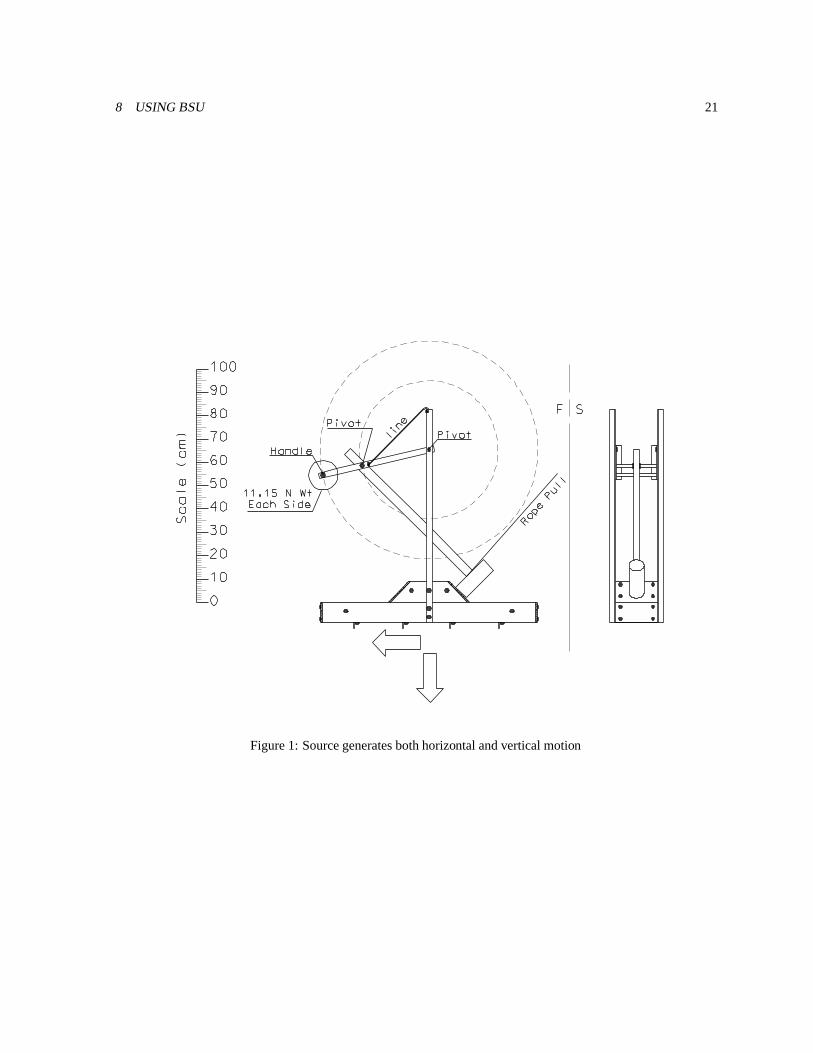
BSU can handle two types of seismic sources for down-hole engineering surveys. A vertical impact hammer sourceis used when the interest is primarily in recording P-waves on the vertical down-hole component. A horizontalhammer serves when the primary interest is in recording SH-waves on the horizontal down-hole components. Inthis example, my 135 degree inclined hammer source is used. This source delivers both horizontal and verticalmotion to the ground. The source is nailed to the soil. The source is shown in Figure 1.

A sign convention for hammer sources has been adopted in BSU. One mentally associates an arrow with theblow. The arrow points in the direction of the blow, and can also be thought of as a unit vector. Thus, in Figure 1, ifwe assume that East is on the right, the hammer blow would be represented by the spherical coordinate designation(270,135)=(azimuth, angle from the vertical). Vertical angles are measured from zenith=0 degrees, to nadir=180degrees. Horizontal, azimuthal angles, are measured from North=0degrees, increasing clockwise (when viewedfrom above), making West=270 degrees. The BSU header stores both the horizontal and vertical angle for thesource.

Data collection with this source involves two source polarizations for each sampled subsurface geophone sta-tion. In a typical survey, the geophone is lowered to the bottom of the hole, clamped with a mechanical bow springclamp (I use a GeoStuff BHG-2 down-hole geophone [3] ), and then dragged up the hole to occupy stations at a0.25 meter interval. As the geophone remains fixed at a station, two separate seismic recordings are stored. Oneis for a source polarization of (270,135), and the other for a source polarization of (90,135). Subtraction of therecords enhances SH-wave motion at the expense of Rayleigh and P-waves (as seen on horizontal components).Summing the two records has the opposite effect. For a more detailed discussion on wave field enhancement, seeMichaels [9].

8.1.2 Down-hole and Reference Geophones

The BSU sign convention for geophones is similar to that for sources. An arrow or unit vector is associatedwith each geophone element. Ground motion in the direction of the arrow will generate a negative voltage at

8 USING BSU 21

Figure 1: Source generates both horizontal and vertical motion

8 USING BSU 22

R

T

Borehole

ReferencePhone

RT

Seismic Source90 270

N

1 m

1 m

o o

Figure 2: Plan view of a typical survey.

the geophone, and be recorded as a negative number on the seismic trace. For a typical moving coil “velocity”phone, this voltage is proportional to particle velocity of the soil, as sensed by the geophone at the point where itis clamped to the soil. Figure 2 shows a plan view of the typical survey for which BSU was written.

There are two 3-component geophones. One is fixed at the surface (or buried very shallow). This referencephone provides a way to monitor variations in the source waveform and recorder triggering. In Figure 2, thehorizontal, R-component of the reference phone is designated (0,90), and the T-component (270,90). The verticalcomponent arrow (not shown) is (0,0), pointing to zenith. The azimuth for the vertical component is meaningless,and so is set to zero for simplicity. The down-hole phone is free to spin on the way down, and so its orientationmust be determined for each down-hole station. This is the job of the Principal Component Analysis (PCA), andwill demonstrate the use of the program, bhod, named for the hodogram in the horizontal plane. The use of thelabels R and T on horizontal components is purely arbitrary in down-hole surveys. You will note that in Figure2, the chirality is not consistent (left handed vs right handed). Your geophones may be quite different, but thesign convention is what is important, and this can be determined by a tap test, or a shallow level where the toolorientation can be observed directly by sight. A very important observation at the end of each survey is to noteand record the bow spring azimuth as the tool exits the hole. On the GeoStuff tool, the spring is aligned withthe R-component. Knowing this direction is essential to establishing a guide vector for the PCA analysis which hasan inherent 180 degree ambiguity. The vertical down-hole component points to zenith in the GeoStuff tool. Not alltools are constructed this way, so you need to check your tool to determine its actual orientation. The down-holevertical component is designated (0,0).

Each seismic trace will have header values for the geophone and source polarization (unit vectors in sphericalcoordinates). These are stored as integers in the BSEGY header. Aside from looking at the include files, theheader definitions can also be reviewed with the man pages. For Fortran definitions use man bsegy . For

C-language definitions, use man c_bsegy . Thus, in C you will find the header structure elements hd.geoaziand hd.geover contain the azimuth and vertical angles of the geophone. The corresponding shot polarization is

8 USING BSU 23

stored in hd.shtazi and hd.shtver.

8.1.3 Sample Data Set from GeoLogan97

If you have downloaded the sample data set, it will be located in directory PREFIX/geologan/1997/15jul/bison,where the PREFIX is your choice of top directory location. The READ.ME file included with the sample Bisondata can be used as a reel header, and documents the experiment and local geology determined by a ConeTechsurvey. To run genvsp, we need to know the experimental geometry as recorded in the observer’s log.

OBSERVER’S LOG

� Global Coordinates of Borehole (x,y,z)=(100.0,100.0, 1.025) in meters. BSU defines “Global” coordinatesas being whatever coordinate system you are working in, usually set by the project you are tying into. Here,I have made up a value of (x,y) to illustrate how the codes work. The z-coordinate is the top of the casingstub from which down-hole measurements are taken. Normally, the casing elevation would be with respectto sea level. However, in this case, it is relative to the ground surface, since the field day did not include asurvey tie in to a bench mark. Note that the z-axis is +UP in global coordinates.

� Local Coordinates of the Source (x,y,z)=(0.0, 1.24, 1.025). The local coordinate system is different, and istaken relative to the bore hole (which is at the origin). Note that the z-axis is + DOWN in local coordinates.The source was oriented with the long axis being East-West, the center of the source was 1.24 meters Northof the bore hole.

� Source Polarization of First (and ALL ODD) Files (azimuth,vertical)=(90,135).

� Source Polarization of Second (and ALL EVEN) Files (azimuth,vertical)=(270,135).

� Local Coordinates of the Reference Phone (x,y,z)=(0.0, 2.17, 1.175). The ground was horizontal aroundthe bore hole (which means that the reference phone was buried 0.15m in this case).

� Depth to Top of Water Table. Normally this would be measured in the bore hole. However, in this case,it appears that the PVC casing was sealed at the bottom, and the water level in the bore hole was not anindication of the local water table.

� Geophone Station Spacing. This was 0.25 meters.

� Deepest Geophone Station. This was for the first two shot records (files LOGN0001 and LOGN0002), andthe phone was 19.25 meters below the casing elevation.

� Shallow most Geophone Station. This was for the last 2 records (files LOGN0145 and LOGN0146). Thephone was at a depth of 1.25 meters below casing elevation.

� Azimuth of bow spring on exiting the bore hole. This was noted at��

, but in the dialog on PCA analysis,a guide vector of

�� was found to require less manual corrections to the bhod.lst file.

8.1.4 Converting Bison Files to BSEGY Format and Setting Geometry

The conversion and geometry setting begins with program genvsp. Change to the directory with the Bison files.From the command line, run the interactive geometry setting program, genvsp by typing: genvsp

The following is the dialog between the program (italics) and user (boxed).Down-hole VSP Pattern GeneratorFor Setting GeometryHandles both Bison and SEG-2 File Formats

8 USING BSU 24

Set Channel Order Switch1=ascending 1,2,3=downhole 4,5,6=reference-1=descending 6,5,4=downhole 3,2,1=reference2=ascending 1,2,3=down 4,5,6=ref,7=load_cell-2=descending 7=load_cell,6,5,4=down 3,2,1=ref1-----------BOREHOLE----------------------------Enter 6 char. name for nez file (ex. STP001)logn01Enter 4 char. LINEID0001Enter Z-Datum: Casing Elevation1.025BOREHOLE LOCATION: Borehole is origin of the local coordinate systemSource and Reference phone locations are x,yrelative to borehole.Following entries will shift every x,y input toa final global coordinate system:Enter Global x-coord. of borehole100.0Enter Global y-coord. of borehole100.0Enter number of sources2FOR THIS SOURCE:Enter Shot Record Names 8char: FirstLOGN0001Enter Shot Record Names 8char: LastLOGN0145LOGN0001LOGN0145Enter Source: x, y, z_sub_CE (positive down)0., 1.27, 1.025Enter Source Polarization: azi, ver90, 135FOR THIS SOURCE:Enter Shot Record Names 8char: FirstLOGN0002Enter Shot Record Names 8char: LastLOGN0146LOGN0002LOGN0146Enter Source: x, y, z_sub_CE (positive down)0., 1.27, 1.025Enter Source Polarization: azi, ver270, 135-----------REFERENCE RECEIVER------------------Enter Reference: x, y, z_sub_CE (positive down)0., 2.17, 1.175Enter Reference Polarizations: R-azi, T-azi

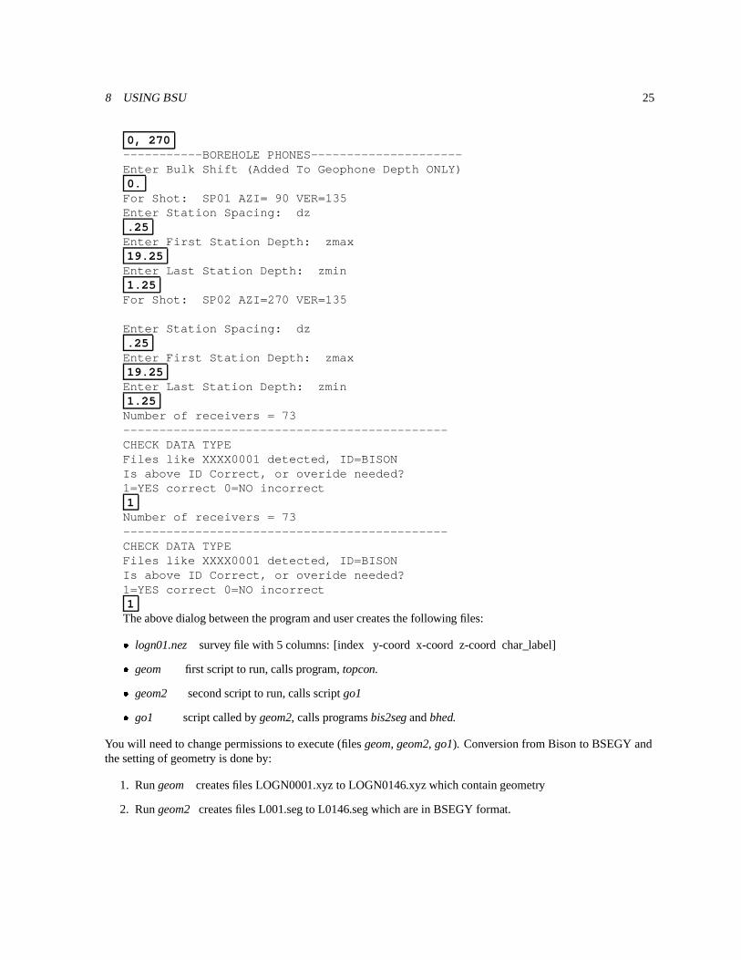
8 USING BSU 25

0, 270-----------BOREHOLE PHONES---------------------Enter Bulk Shift (Added To Geophone Depth ONLY)0.For Shot: SP01 AZI= 90 VER=135Enter Station Spacing: dz.25Enter First Station Depth: zmax19.25Enter Last Station Depth: zmin1.25For Shot: SP02 AZI=270 VER=135

Enter Station Spacing: dz.25Enter First Station Depth: zmax19.25Enter Last Station Depth: zmin1.25Number of receivers = 73---------------------------------------------CHECK DATA TYPEFiles like XXXX0001 detected, ID=BISONIs above ID Correct, or overide needed?1=YES correct 0=NO incorrect1Number of receivers = 73---------------------------------------------CHECK DATA TYPEFiles like XXXX0001 detected, ID=BISONIs above ID Correct, or overide needed?1=YES correct 0=NO incorrect1

The above dialog between the program and user creates the following files:

� logn01.nez survey file with 5 columns: [index y-coord x-coord z-coord char_label]

� geom first script to run, calls program, topcon.

� geom2 second script to run, calls script go1

� go1 script called by geom2, calls programs bis2seg and bhed.

You will need to change permissions to execute (files geom, geom2, go1). Conversion from Bison to BSEGY andthe setting of geometry is done by:

1. Run geom creates files LOGN0001.xyz to LOGN0146.xyz which contain geometry

2. Run geom2 creates files L001.seg to L0146.seg which are in BSEGY format.

8 USING BSU 26

8.1.4.1 Post genvsp processing steps

1. Removing the *.xyz files if they appear OK. These are in bhed format. The bhed program was run in scriptgo1 called by geom2.

2. Removing the *.lst files if they appear OK. These files are created by bis2seg and contain a listing of theBison file header information. Program, bis2seg, was run in the go1 script called by geom2.

3. Gzip the Bison files to save disk space.

4. Move the L*.seg files to a new directory. For example: mv L*.seg ../seg assuming that the directoryPREFIX/geologan/1997/15jul/seg exists.

The newly created *.seg files in BSEGY format have the majority of the header information set. What is missingis the horizontal component orientation of the down-hole tool. For that, we must run programs genbhod and bhod.

8.1.5 Determining Down-hole Tool Orientation by PCA

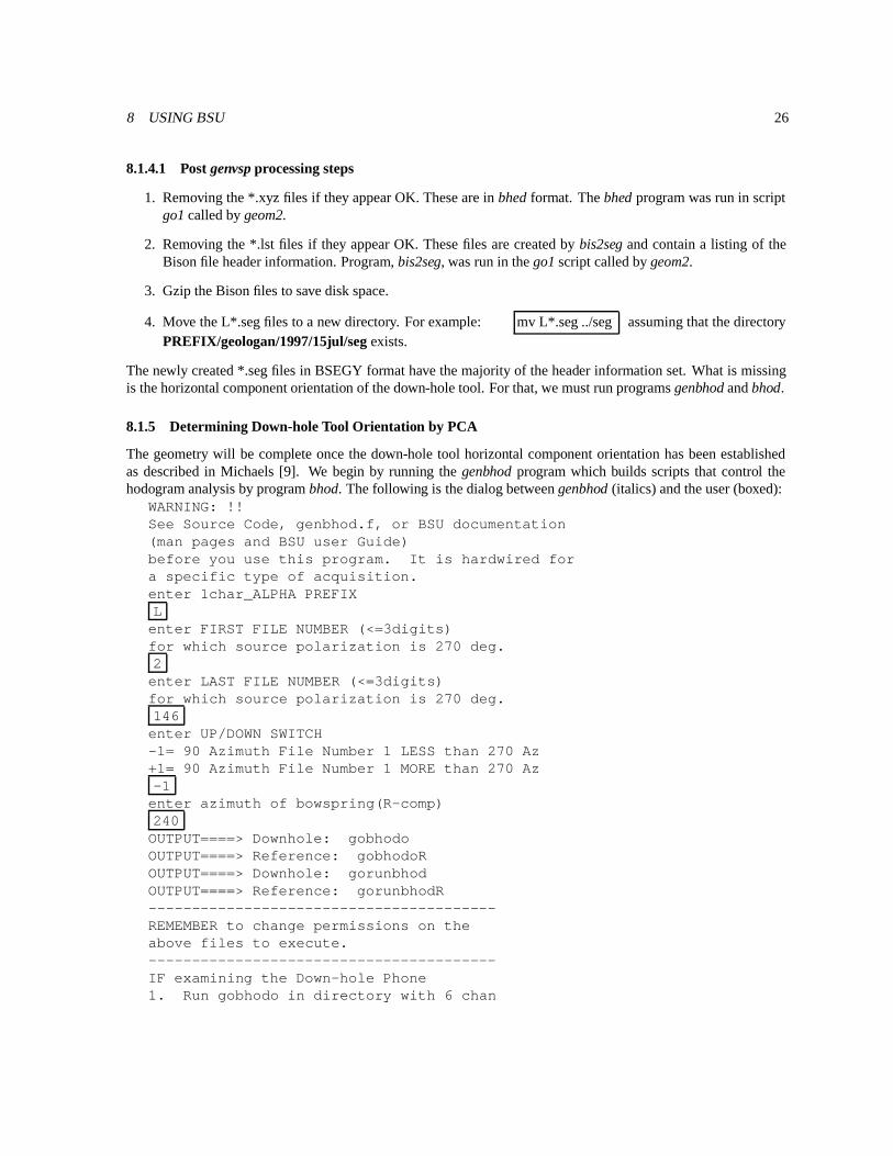
The geometry will be complete once the down-hole tool horizontal component orientation has been establishedas described in Michaels [9]. We begin by running the genbhod program which builds scripts that control thehodogram analysis by program bhod. The following is the dialog between genbhod (italics) and the user (boxed):

WARNING: !!See Source Code, genbhod.f, or BSU documentation(man pages and BSU user Guide)before you use this program. It is hardwired fora specific type of acquisition.enter 1char_ALPHA PREFIXLenter FIRST FILE NUMBER (<=3digits)for which source polarization is 270 deg.2enter LAST FILE NUMBER (<=3digits)for which source polarization is 270 deg.146enter UP/DOWN SWITCH-1= 90 Azimuth File Number 1 LESS than 270 Az+1= 90 Azimuth File Number 1 MORE than 270 Az-1enter azimuth of bowspring(R-comp)240OUTPUT====> Downhole: gobhodoOUTPUT====> Reference: gobhodoROUTPUT====> Downhole: gorunbhodOUTPUT====> Reference: gorunbhodR----------------------------------------REMEMBER to change permissions on theabove files to execute.----------------------------------------IF examining the Down-hole Phone1. Run gobhodo in directory with 6 chan

8 USING BSU 27

records (3 down, 3 reference phones)2. Run gorunbhod in directory with filesthat are named hxxxyyy.seg----------------------------------------IF examining the Reference Phone1. Run gobhodoR in the directory withthe 6 channel records.2. Run gorunbhodR in the directory withfiles that are named rxxxyyy.seg

Because the tool is fixed for both source polarizations, there will be half as many orientation determinations as thereare seismic files. The tips at the bottom of the dialog are reminders about which scripts are for what purpose. In anormal case, one generally is only interested in the down-hole tool orientation, and will only run scripts gobhodoand gorunbhod. If you are interested in viewing the actual rotation of the radiation from the source with time, thenyou will run the other two scripts, gobhodoR and gorunbhodR (the upper case “R” being a reminder that these arefor the fixed reference phone). The following steps are recommended:

1. Make a new directory for the hodogram analysis under the current “seg” directory. For example, mkdir hodowill do this nicely.

2. Run the script, gobhodo in the current “seg” directory. This creates a lot of files.

3. Move the files beginning with “h” to the directory “hodo” created in step (1). mv h*.seg hodo

4. Remove the bscl generated files. rm bscl*

5. Copy gorunbhod to the “hodo” directory. cp gorunbhodhodo

6. Change into the hodo directory and run gorunbhod. The important file to save is bhod.lst. It contains a listof the file numbers with tool orientations. Copy bhod.lst back to the “seg” directory.

7. Run the script, mergeplots, provided in the script directory of the distribution. This merges all the PostScript(*.ps) files into a single PDF file for viewing in a program like acroread (Adobe Acrobat).

8. Remove the *.ps files, and view the file, merge.pdf .

9. Look for �� reversals in polarity, particularly if the tool had to be released during any part of the survey(and hence was free to spin). Sometimes, a slight change in the guide vector azimuth will help on a secondattempt.

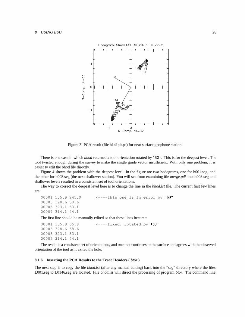
Figure 3 shows the plot for the files L141.seg and L142.seg. The SH-wave enhancement involved subtracting theeven from the odd files (see gobhodo script). The result was file h141.seg. It is this file, h141.seg which was thensubjected to PCA analysis by program bhod.

Since this is a shallow station, it corresponds to the observed orientation of the bow spring when the tool exitedthe hole. Without the guide vector (set at

� �� in the dialog above), the resulting R-component direction could

easily have been rotated by �� due to the inherent ambiguity in the eigenvector solution. The line in the filebhod.lst corresponding to this station is: 00141 209.5 299.5 from which you can see the meaning of the 3columns. The first column corresponds to the file number, the second column the R-component azimuth, and thethird column is the T-component azimuth. The values will be truncated to integers when written to the headers byprogram btor.

8 USING BSU 28

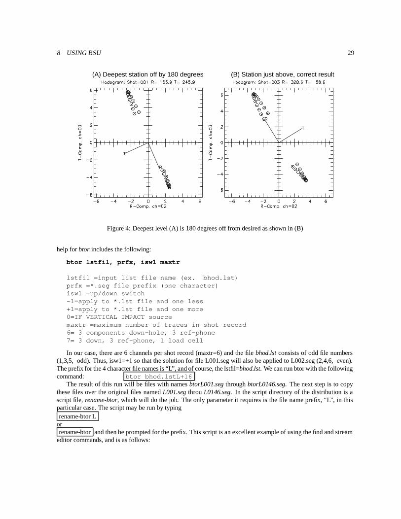
Figure 3: PCA result (file h141plt.ps) for near surface geophone station.

There is one case in which bhod returned a tool orientation rotated by �� . This is for the deepest level. Thetool twisted enough during the survey to make the single guide vector insufficient. With only one problem, it iseasier to edit the bhod file directly.

Figure 4 shows the problem with the deepest level. In the figure are two hodograms, one for h001.seg, andthe other for h003.seg (the next shallower station). You will see from examining file merge.pdf that h003.seg andshallower levels resulted in a consistent set of tool orientations.

The way to correct the deepest level here is to change the line in the bhod.lst file. The current first few linesare:

00001 155.9 245.9 <----this one is in error by � � � �

00003 328.6 58.600005 323.1 53.100007 314.1 44.1

The first line should be manually edited so that these lines become:

00001 335.9 65.9 <----fixed, rotated by ��

00003 328.6 58.600005 323.1 53.100007 314.1 44.1

The result is a consistent set of orientations, and one that continues to the surface and agrees with the observedorientation of the tool as it exited the hole.

8.1.6 Inserting the PCA Results to the Trace Headers ( btor )

The next step is to copy the file bhod.lst (after any manual editing) back into the “seg” directory where the filesL001.seg to L0146.seg are located. File bhod.lst will direct the processing of program btor. The command line

8 USING BSU 29

(A) Deepest station off by 180 degrees (B) Station just above, correct result

Figure 4: Deepest level (A) is 180 degrees off from desired as shown in (B)

help for btor includes the following:

btor lstfil, prfx, isw1 maxtr

lstfil =input list file name (ex. bhod.lst)prfx =*.seg file prefix (one character)isw1 =up/down switch-1=apply to *.lst file and one less+1=apply to *.lst file and one more0=IF VERTICAL IMPACT sourcemaxtr =maximum number of traces in shot record6= 3 components down-hole, 3 ref-phone7= 3 down, 3 ref-phone, 1 load cell

In our case, there are 6 channels per shot record (maxtr=6) and the file bhod.lst consists of odd file numbers(1,3,5, odd). Thus, isw1=+1 so that the solution for file L001.seg will also be applied to L002.seg (2,4,6, even).The prefix for the 4 character file names is “L”, and of course, the lstfil=bhod.lst. We can run btor with the followingcommand: btor bhod.lstL+16

The result of this run will be files with names btorL001.seg through btorL0146.seg. The next step is to copythese files over the original files named L001.seg throu L0146.seg. In the script directory of the distribution is ascript file, rename-btor, which will do the job. The only parameter it requires is the file name prefix, “L”, in thisparticular case. The script may be run by typingrename-btor L

orrename-btor and then be prompted for the prefix. This script is an excellent example of using the find and stream

editor commands, and is as follows:

8 USING BSU 30

#!/bin/sh #Script to rename files after btor process#overwrite pxxx.seg files, p=prefix# Author: P. Michaels Date:April 2002 See GNU Licenseif test "$1" = ”thenecho ’Enter 1 character prefix’echo ’Example: w’echo ’ for files btorw001.seg, btorw002.seg, etc...’read PRFXelsePRFX=$1fifind -name "$PRFX*.seg" | \sed s/’\.\/’/’ ’/g | \gawk ’{print "mv","btor"$1,$1}’ \>go-renamechmod +x go-rename./go-renameecho "btor files renamed"

Once the script has the prefix character, a find command is issued to get a list of the files L*.seg, and this ispiped through sed editor to remove the leading “.” and “/” characters. The result is piped through gawk (the GNUversion of awk) to construct move commands which are written to a file, go-rename, that file is made executable,and then executed.

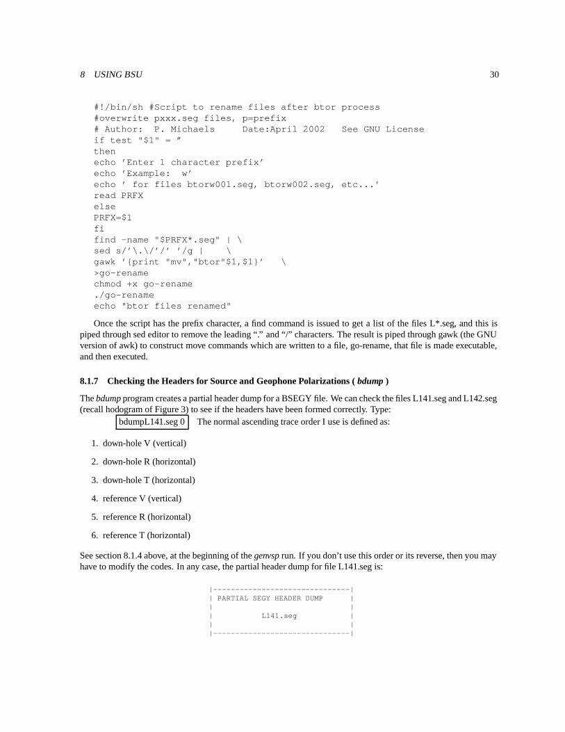
8.1.7 Checking the Headers for Source and Geophone Polarizations ( bdump )

The bdump program creates a partial header dump for a BSEGY file. We can check the files L141.seg and L142.seg(recall hodogram of Figure 3) to see if the headers have been formed correctly. Type:

bdumpL141.seg 0 The normal ascending trace order I use is defined as:

1. down-hole V (vertical)

2. down-hole R (horizontal)

3. down-hole T (horizontal)

4. reference V (vertical)

5. reference R (horizontal)

6. reference T (horizontal)

See section 8.1.4 above, at the beginning of the genvsp run. If you don’t use this order or its reverse, then you mayhave to modify the codes. In any case, the partial header dump for file L141.seg is:

|-------------------------------|| PARTIAL SEGY HEADER DUMP || || L141.seg || ||-------------------------------|

8 USING BSU 31

-----------------------------------------------------------------------------------Length = 2000 samples | Shot Elevation = 0.0Sample Interval = 0.00025 sec. | Shot Depth = 0.0Delay Time = 0 msec. | Up Hole Time = 0 msecLow Cut Filter = 4 Hz. | Shot X-COORD = 100.00High Cut Filter = 1000 Hz. | Shot Y-COORD = 101.27Line ID: 0001 | Shot Date (year.day) = 1997.0715Shot Orientation: | Shot Time (hr:min) = 11:48Azimuth= 90 Deg. Vertical=135 Deg. | Charge Size (grams)= 0

-----------------------------------------------------------------------------------TRACE|SHOT| STATION | OFFSET| RECEIVER |VERT|1STBRK|K-GAIN|AZI|VER|# |REC.|SHOT REC | | ELEV. X-COORD Y-COORD |FOLD|(SEC.)| (dB) | | |-----|----|---------|-------|----------------------------|--|------|------|---|---|1 | 141| 001 421 | 1.46 | -0.73 100.00 100.00 | 3|0.0000| 20 | 0 | 0 |2 | 141| 001 422 | 1.46 | -0.73 100.00 100.00 | 3|0.0000| 20 |209| 90|3 | 141| 001 423 | 1.46 | -0.73 100.00 100.00 | 3|0.0000| 20 |299| 90|4 | 141| 001 424 | 0.91 | -0.15 100.00 102.17 | 3|0.0000| 0 | 0| 0|5 | 141| 001 425 | 0.91 | -0.15 100.00 102.17 | 3|0.0000| 0 | 0| 90|6 | 141| 001 426 | 0.91 | -0.15 100.00 102.17 | 3|0.0000| 0 |270| 90|

Note that the two down-hole horizontal traces, 2 and 3, have azimuth R=� ��

and T=��

as determined inthe Figure 3 hodogram. The dump for L142.seg is almost identical to that above, the only differences being thesource polarization (which is azimuth=

�� rather than

�� as show here), and of course the time of day.

8.1.8 Rotating the Horizontal Data into Alignment with Source ( genbrot and brot )

Once the headers have been updated with the down-hole tool orientation, the next step is to rotate the horizontaldata into a single orientation. This removes any spin that has occurred while dragging the tool up the hole. Thegenbrot program is run interactively to generate a script which can then be executed. The script automates runningprogram brot on all the shot gathers. Program genbrot is set up to process data according to the channel definitionsof section 8.1.7 above. Thus, only the data on traces 2 and 3 are rotated.

The program brot is quite flexible in how to rotate the data. Program genbrot, however, makes a single choiceand would have to be modified if that did not suit a user’s needs. The default choice imposed by genbrot is to alignthe data so that the T-component down-hole becomes aligned with the T-component of the reference phone. Thisparticular rotation was based on the decision to align the T-component of the reference phone with the long axis ofthe source (see Figure 2).

The result of the above decisions is to align trace 3 with the long axis of the source, to the extent thatthe radiation from the source is also aligned with the long axis of the source. While one might think that thesource shown in Figure 1 would radiate SH-motion polarized parallel to the long axis of the source (aligned withthe hammer blows), it appears that variations in soil stiffness under the source can cause a couple, twisting thepolarization axis of the radiation slightly out of alignment with the source axis (see Michaels [9] ). Thus, a moreproper statement might be that the horizontal data are aligned with the major axis of the source radiationpolarization ellipse, rather than with the long axis of the source itself.

As a final caution, if a user has not acquired the data with the geometry as shown in Figure 2, the blinduse of the program genbhod may produce unwanted and unexpected results. There are many ways to set upthe source and reference phone about the bore hole (both in location and component orientation). My choice wasdesigned to permit SH-waves to be recorded from depth to the surface, with as little interference as possible fromother wave fields.

The dialog for genbhod would be as follows:Enter alpha prefix (char) of *.seg data to be rotated

EXAMPLE: if enter 1, then files 1001.seg to 1010.seg

8 USING BSU 32

would be processed if sequencenumbers 1 and 10 entered nextL...LEnter first file number to process1Enter last file number to process146Output in file===>gobrotThe next step would be to make the bash script, gobrot, executable: chmod+xgobrotAfter running gobrot, you will have files named brotL001.seg through brotL0146.seg. These data are rotated

to the standard orientation described above. Not only are the data rotated, but the headers have been changed fortraces 2 and 3 to reflect their new azimuths.

8.1.8.1 Post brot processing steps With so many files, both rotated and unrotated in the same directory, it canget a bit messy. The following steps are recommended.

1. Make a new directory for the rotated data. For example, mkdirbrot

2. Move the rotated data to the new directory mvbrot*.segbrot

3. Clean up the current directory:a). remove the list files rmbrot*.lstbrot

b). gzip the unrotated data to save space gzip*.seg

4. Change to the “brot” directory, since the next steps are executed on the rotated data.

8.1.9 Sorting and Merging to Common Receiver Component Gathers

What we would like to look at is not a multiplexed display of different components, but rather a gather of allone type of component. For P-waves, our first choice would be to gather all the down-hole vertical componentdata into a single file (trace #1 from all the files). For the SH-waves, we will want to gather all the down-holeT-component data (trace #3 from all the files). Included in the BSU distribution is a bash script, Merge, whichproduces some of these common component gathers. An alternative script is Merge-all (Appendix B) whichgenerates all combinations of sum or difference on all components. In addition to gathering a component, theMerge script also computes wave field enhancements and wave shaping to remove source variations monitored bythe reference phone. Begin by copying the Merge script into your “brot” directory which contains the brot*.segfiles. NOTE: For vertical component sources (only one polarization) see script Merge2 (in the scripts directory andAppendix C). Merge2 is designed for 7 component recording (load cell on hammer is 7th signal). This script canalso be modified for vertical impact sources without a load cell.

8.1.10 Edit Merge Script for the Specific Down-hole Survey

Since several survey details are likely to vary from one bore hole to the next, you must edit a few lines of the file,Merge. These lines are near the top of the file and are reproduced below. The boxed values will need to be changed.

#set -x#...define parameters YOU MUST DEFINE THESE FOR EACH NEW SURVEY# SINCE IT IS LIKELY THAT THE NUMBER OF RECORDS

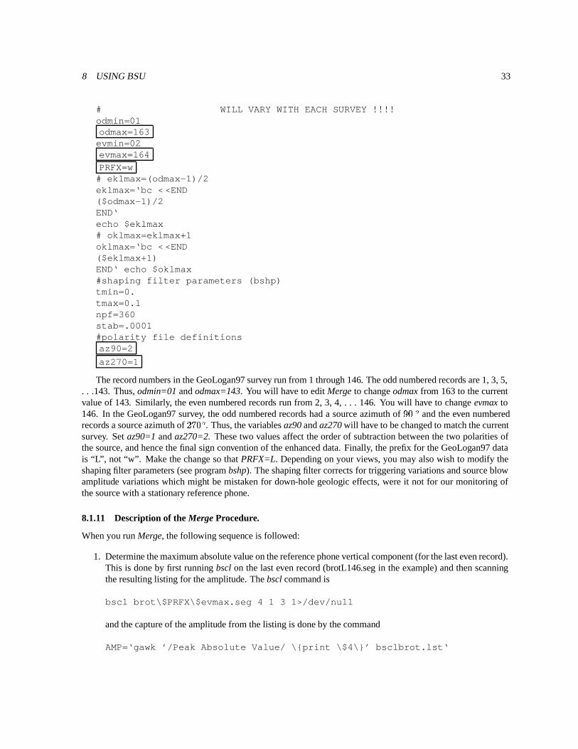
8 USING BSU 33

# WILL VARY WITH EACH SURVEY !!!!odmin=01odmax=163evmin=02evmax=164

PRFX=w# eklmax=(odmax-1)/2eklmax=‘bc <<END($odmax-1)/2END‘echo $eklmax# oklmax=eklmax+1oklmax=‘bc <<END($eklmax+1)END‘ echo $oklmax#shaping filter parameters (bshp)tmin=0.tmax=0.1npf=360stab=.0001#polarity file definitionsaz90=2

az270=1

The record numbers in the GeoLogan97 survey run from 1 through 146. The odd numbered records are 1, 3, 5,. . .143. Thus, odmin=01 and odmax=143. You will have to edit Merge to change odmax from 163 to the currentvalue of 143. Similarly, the even numbered records run from 2, 3, 4, . . . 146. You will have to change evmax to146. In the GeoLogan97 survey, the odd numbered records had a source azimuth of

�� and the even numbered

records a source azimuth of��

. Thus, the variables az90 and az270 will have to be changed to match the currentsurvey. Set az90=1 and az270=2. These two values affect the order of subtraction between the two polarities ofthe source, and hence the final sign convention of the enhanced data. Finally, the prefix for the GeoLogan97 datais “L”, not “w”. Make the change so that PRFX=L. Depending on your views, you may also wish to modify theshaping filter parameters (see program bshp). The shaping filter corrects for triggering variations and source blowamplitude variations which might be mistaken for down-hole geologic effects, were it not for our monitoring ofthe source with a stationary reference phone.

8.1.11 Description of the Merge Procedure.

When you run Merge, the following sequence is followed:

1. Determine the maximum absolute value on the reference phone vertical component (for the last even record).This is done by first running bscl on the last even record (brotL146.seg in the example) and then scanningthe resulting listing for the amplitude. The bscl command is

bscl brot\$PRFX\$evmax.seg 4 1 3 1>/dev/null

and the capture of the amplitude from the listing is done by the command

AMP=‘gawk ’/Peak Absolute Value/ \{print \$4\}’ bsclbrot.lst‘

8 USING BSU 34

2. A list of reduced file names is created with the file command. Thus, FILE=L001 L002 L003 . . L146 whenthe following command is executed:

FILE=‘find brot*seg | sed s/\.seg/”/g |sed s/brot/”/g‘

3. The list in FILE is then directs a do loop which scales each brotL*.seg file first to unity maximum absoluteamplitude on the reference vertical component, followed by a rescaling that makes all the files in the listend up having the same maximum absolute value on their respective vertical reference phone signals. Thissingle new value is of course the AMP value captured in step (1) above.

4. The newly formed scaled versions all have been scaled to the same peak signal on their vertical reference,and this is dominated by the Near Field and Rayleigh waves. The goal is to null out the Rayleigh wave, andfocus on the body waves down-hole. At this point, a sequence of bmrg runs are made to collect commonreceiver gathers. The files created are:a) rfv1.seg and rfv2.seg [reference, Vertical for shot azimuths 270 and 90 degrees respectively]b) rft1.seg and rft2.seg [reference, T-comp. for shot azimuths 270 and 90 degrees respectively]c) swt1.seg and swt2.seg [down-hole, T-comp. for shot azimuths 270 and 90 degrees respectively]d) swv1.seg and swv2.seg [down-hole, Vertical for shot azimuths 270 and 90 degrees respectively]

5. Enhancements without shaping filters are computed by subtracting the az270 files from the az90 files (SH-wave enhancement), or summing the az270 and az90 files (P-wave enhancement). The resulting output filesare:a) twav.seg [SH-wave enhanced, viewed on the T-component down-hole]b) pwav.seg [P-wave enhanced, viewed on the Vertical component down-hole]

6. The shaping filter versions of enhanced P- and SH-waves is done by first running bshp on the referencephone traces, matching each reference to a target waveform, and then applying the filters on a second passto the down-hole data. Thus, filter design is on the reference phone data, application is to both the referencephone (for QC) and to the down-hole (removes source fluctuations from down-hole data). The resulting filecomparable to step (5) are:a) twave.seg [SH-wave enhanced, viewed on the T-component down-hole]b) pwave.seg [P-wave enhanced, viewed on the Vertical component down-hole]Note: The only difference in the names is the extra letter “e”.

In summary, the files twav.seg and pwav.seg are enhanced SH- and P-waves, without any shaping filters. The filestwave.seg and pwave.seg have the additional Wiener Least Squares shaping based on observations of the referencephone.

8.1.12 Plotting the Results from Merge

Initial plots produced by a call to gplt in Merge can be improved on by using Seismic Unix (SU). The BSUdistribution includes some scripts, xPlot and psPlot, which call SU programs for plotting in an X-window or as aPostScript file. Figure 5 illustrates how plots made with psPlot can be combined in Xfig with the results of a directpush survey by ConeTec. The ConeTec survey was done in preparation for the field day event.

The twave.seg file has been trace equalized by the program bequ. If each trace were not individually scaled, thelarge variation in amplitude would result in the deep data disappearing below the visible threshold. The SH-wavearrives just before the 0.1 second timing line at the bottom of the survey. A faint, unidentified wave arrives at about.05 seconds (between what may be the P- and SH-waves).

Figure 6 shows the pwav.seg file, also processed by bequ. In this case, the scaling was based on the data from 0to .025 seconds. What may be the P-wave arrives at about .02 seconds at the bottom of the survey. The file named

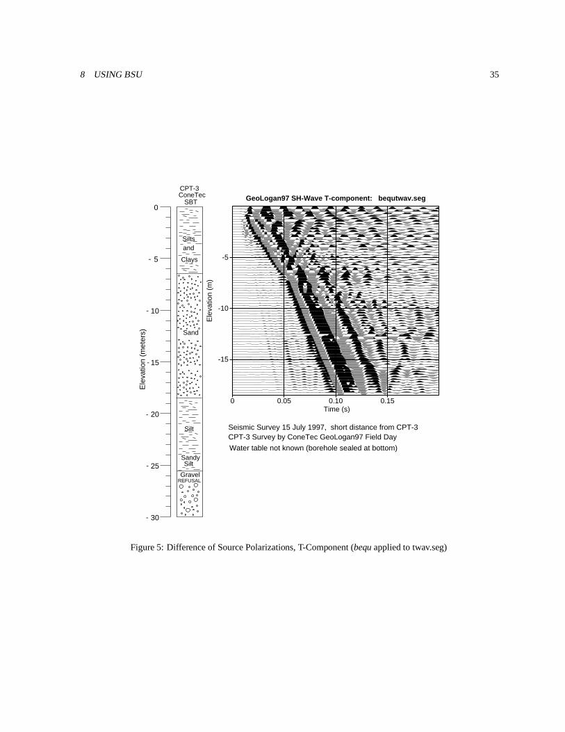
8 USING BSU 35

Clays

andSilts

Sand

SBT

CPT-3ConeTec

30

25

20

15

5

10

0

Silt

SandySilt

GravelREFUSAL

Ele

vatio

n (m

eter

s)

-

-

-

-

-

-

0 0.05 0.10 0.15 Time (s)

-15

-10

-5

Ele

vatio

n (m

)

GeoLogan97 SH-Wave T-component: bequtwav.seg

Seismic Survey 15 July 1997, short distance from CPT-3CPT-3 Survey by ConeTec GeoLogan97 Field Day

Water table not known (borehole sealed at bottom)

Figure 5: Difference of Source Polarizations, T-Component (bequ applied to twav.seg)

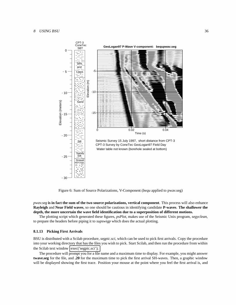
8 USING BSU 36

Clays

andSilts

Sand

SBT

CPT-3ConeTec

30

25

20

15

5

10

0

Silt

SandySilt

GravelREFUSAL

Ele

vatio

n (m

eter

s)

-

-

-

-

-

-

0 0.02 0.04 Time (s)

-15

-10

-5

Ele

vatio

n (m

)

GeoLogan97 P-Wave V-component: bequpwav.seg

Seismic Survey 15 July 1997, short distance from CPT-3CPT-3 Survey by ConeTec GeoLogan97 Field DayWater table not known (borehole sealed at bottom)

Figure 6: Sum of Source Polarizations, V-Component (bequ applied to pwav.seg)

pwav.seg is in fact the sum of the two source polarizations, vertical component. This process will also enhanceRayleigh and Near Field waves, so one should be cautious in identifying candidate P-waves. The shallower thedepth, the more uncertain the wave field identification due to a superposition of different motions.

The plotting script which generated these figures, psPlot, makes use of the Seismic Unix program, segyclean,to prepare the headers before piping it to supswigp which does the actual plotting.

8.1.13 Picking First Arrivals

BSU is distributed with a Scilab procedure, segpic.sci, which can be used to pick first arrivals. Copy the procedureinto your working directory that has the files you wish to pick. Start Scilab, and then run the procedure from withinthe Scilab text window exec(’segpic.sci’);

The procedure will prompt you for a file name and a maximum time to display. For example, you might answertwave.seg for the file, and .20 for the maximum time to pick the first arrival SH-waves. Then, a graphic windowwill be displayed showing the first trace. Position your mouse at the point where you feel the first arrival is, and

8 USING BSU 37

click with your left mouse button. Only the lateral position is read from the mouse click, so you don’t have tobe concerned about the vertical placement of the mouse, other than it be somewhere inside the plot window. Theprocedure moves on to the next trace after the click. This is a rather simple routine, and you can’t go backwards.After all the traces have been picked, the procedure writes the picks to a file, (trace #, pick time) pairs. This file isalways called pics.pic. You will probably wish to move it to another name, say twave.pic.

The picks can be written to the file trace headers by running bpic in your X-term window. For demonstration,the I have picked file twave.seg, and in the interest of better signal to noise, picked not the first motion, but the zerocrossing from the first peak to trough of the first arrival SH-wave. This occurs about .005 seconds after the firstmotion. The picks are inserted into headers with the command,

bpic twave.seg 1 pwave.pic -.005

The last argument, -.005, shifts the value in the twave.pic file to a point earlier in time, where the first motionis located. The output file is called, bpictwav.seg. You can then move this to replace the original file, twave.seg,thus completing the operation. Now twave.seg will have the picks in the headers.

8.1.13.1 Quality control of picks The easy way to QC picks is to align the data on a constant time line usingthe picks in the headers for static shifts. The program, bshf, will do this. For example, type the command

bshf twave.seg 0 1 .02

This will align the data on the .02 second timing line by applying static shifts equal to the negative of the pickvalue. Figure 7 shows this process (picking, insertion to headers, and alignment in time for QC) at the final align-ment step. If a pick were bad, it would be evident by a misalignment of the corresponding trace, relative to itsneighbors. In Figure 7, all the picks look good.

It is evident that the propagating wavelet is changing shape (first motion peak stretches in time with increas-ing distance from the source). Such wavelet stretch may be interpreted as inelastic wave propagation, perhapsconsistent with a viscoelastic, Kelvin-Voigt, constitutive model. Despite the expected velocity dispersion, one candetermine a group velocity for the frequencies which dominate the amplitude spectrum of the signal.

8.1.14 Vertical Time and Observed Travel Time Inversion (vfitw.sci, vplot.sci, bvsp)

The BSU distribution includes a procedure, vfitw.sci, which reads the picks in the trace headers of a BSEGY dataset. The procedure projects the picks to the vertical, and prompts the user to select the top and bottom of an intervalfor a least squares linear fit. The resulting slope yields an estimate of the vertical group propagation velocity. Ifthe results of vfitw.sci are written to disk, a second program, vplot.sci, may be used to plot the solutions with moreuser control. Exporting the plot to Xfig format will allow one to draft on the final figure.

Figure 8a is the vplot.sci generated plot of a two interval analysis of the T-component data. A significantincrease in group velocity occurs at the transition from silt-clay soil to the sand (soil types determined by SoilBehavior Type (SBT) of the ConeTec survey made available at GeoLogan97). An alternative to working withvertical times is program bvsp which does an inversion based on 2 layers over a half-space. Bvsp works withthe observed times, and solves for refracted and direct raypaths in a non-linear ray tracing scheme (horizontalboundaries). The bvsp result is shown in Figure 8b (after 40 iterations).

It should be remembered that the ConeTec and seismic survey were done at different times of year (ConeTec inNovember 1996, seismic in July 1997). Further, the two surveys were in the same general area, but not at exactlythe same location. The lateral separation of the two could easily be 50 meters or more. For that reason, exact depthcorrelations are not possible.

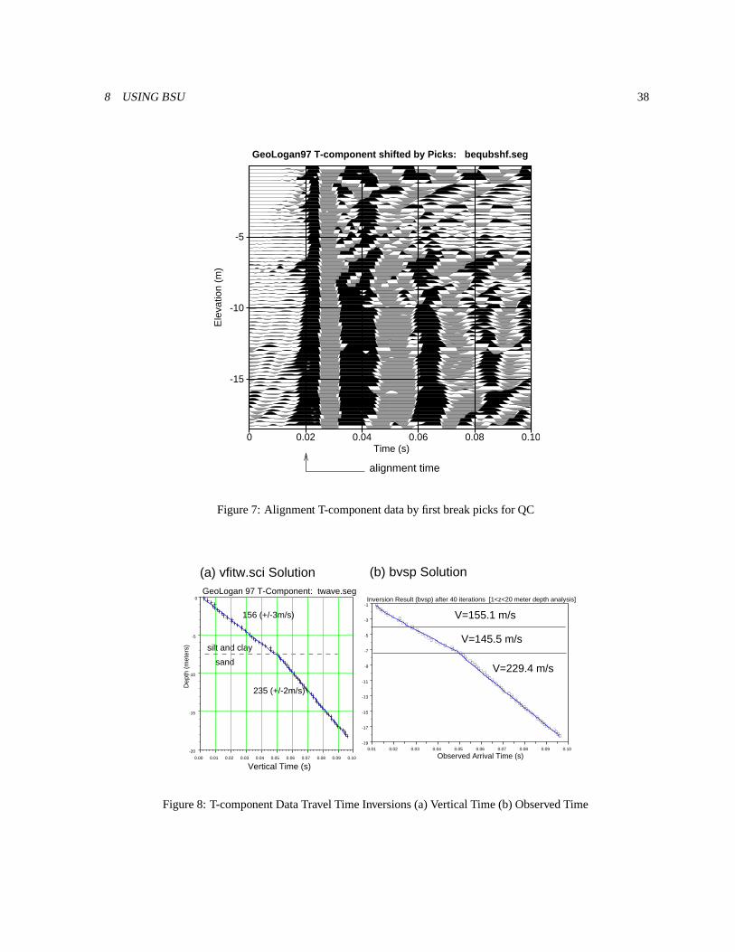
8 USING BSU 38

alignment time

0 0.02 0.04 0.06 0.08 0.10 Time (s)

-15

-10

-5

Ele

vatio

n (m

)

GeoLogan97 T-component shifted by Picks: bequbshf.seg

Figure 7: Alignment T-component data by first break picks for QC

V=155.1 m/s

V=145.5 m/s

V=229.4 m/s

Inversion Result (bvsp) after 40 iterations [1<z<20 meter depth analysis]

Observed Arrival Time (s)

(b) bvsp Solution

silt and clay

sand

GeoLogan 97 T-Component: twave.seg

(a) vfitw.sci Solution

0.01 0.02 0.03 0.04 0.05 0.06 0.07 0.08 0.09 0.10-19

-17

-15

-13

-11

-9

-7

-5

-3

-1

⊕⊕⊕⊕⊕⊕⊕⊕⊕⊕⊕⊕⊕⊕⊕⊕⊕⊕⊕⊕

⊕⊕⊕⊕⊕

⊕⊕⊕⊕⊕⊕⊕⊕⊕

⊕⊕⊕⊕⊕⊕⊕⊕⊕⊕⊕⊕⊕

⊕⊕⊕⊕⊕⊕⊕⊕⊕⊕⊕⊕⊕⊕⊕

⊕⊕⊕⊕⊕⊕⊕

0.00 0.01 0.02 0.03 0.04 0.05 0.06 0.07 0.08 0.09 0.10

-20

-15

-10

-5

0.

235 (+/-2m/s)

156 (+/-3m/s)

Vertical Time (s)

Dep

th (

met

ers)

Figure 8: T-component Data Travel Time Inversions (a) Vertical Time (b) Observed Time

8 USING BSU 39

8.1.15 Determination of Stiffness and Damping

The programs bvas and bamp are used to measure the velocity dispersion and amplitude decay as a function offrequency. These measurements are inverted for material stiffness and damping by Scilab procedure cainv3.sciaccording to a method described by Michaels [7]. The constitutive model is often referred to as the Kelvin orKelvin-Voigt solid.

8.1.15.1 Governing Differential Equation The PDE relevant to 1-D wave propagation is given by�� (1)

where “u” is particle displacement, “t” is time, “x” is the coordinate in the direction of wave propagation, �� isthe stiffness

�� , and � � is the damping�� . Equation (1) reduces to the elastic wave equation when the

damping value, � � � �. In that case, the phase velocity is constant for all frequencies, and the wave does not

experience any decay (for a 1-D plane wave). In the elastic case, the phase velocity will be � �� .In the more general case, � ��

, and there will be both velocity dispersion and exponential, inelastic ampli-tude decay. A solution of equation (1) is�! "�$#%�'& �)( *,+ '-/.0��&!132 465$ "78��-�9��'&�#where the wavenumber is complex and given by

7 ��: . .Michaels [7] shows that the inelastic decay of a plane wave will be given by

. � � � ; 9 � � � � 9 � � & � � ; �where

9is angular frequency (rad/s) and the quantity, D, is given by

; � �=< ��> � � � 9 � � ��@?�A (2)

The phase velocity, c, varies with frequency according to the following relationship

B � � 9C� � �; . A (3)

The values for �D and � � can be expressed in terms of the following :

��FE 7$��-G.0�IH�9C� J7 � � . � & � #(4)

and � � � � .$789 J7 � � . � & � A (5)

Determination of � and � � is by nonlinear joint inversion of the phase velocity, c, and inelastic decay,.

, overa range of frequencies. The inversion is currently performed in the Scilab procedure, cainv3.sci. Initial estimatesof stiffness and damping are obtained at the frequency corresponding to the largest

.measured by bamp. First, �

is found by evaluation of equation (4). In that computation,7 �LK M . Then, � � is estimated from equation (5).

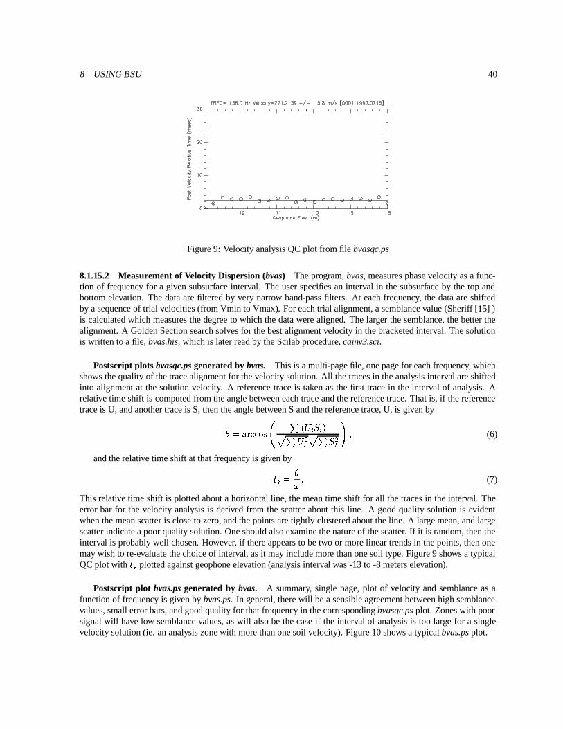
8 USING BSU 40

Figure 9: Velocity analysis QC plot from file bvasqc.ps

8.1.15.2 Measurement of Velocity Dispersion (bvas) The program, bvas, measures phase velocity as a func-tion of frequency for a given subsurface interval. The user specifies an interval in the subsurface by the top andbottom elevation. The data are filtered by very narrow band-pass filters. At each frequency, the data are shiftedby a sequence of trial velocities (from Vmin to Vmax). For each trial alignment, a semblance value (Sheriff [15] )is calculated which measures the degree to which the data were aligned. The larger the semblance, the better thealignment. A Golden Section search solves for the best alignment velocity in the bracketed interval. The solutionis written to a file, bvas.his, which is later read by the Scilab procedure, cainv3.sci.

Postscript plots bvasqc.ps generated by bvas. This is a multi-page file, one page for each frequency, whichshows the quality of the trace alignment for the velocity solution. All the traces in the analysis interval are shiftedinto alignment at the solution velocity. A reference trace is taken as the first trace in the interval of analysis. Arelative time shift is computed from the angle between each trace and the reference trace. That is, if the referencetrace is U, and another trace is S, then the angle between S and the reference trace, U, is given by� �� 232 465 � � �� & � � � � � �� # (6)

and the relative time shift at that frequency is given by� � � �9 A (7)

This relative time shift is plotted about a horizontal line, the mean time shift for all the traces in the interval. Theerror bar for the velocity analysis is derived from the scatter about this line. A good quality solution is evidentwhen the mean scatter is close to zero, and the points are tightly clustered about the line. A large mean, and largescatter indicate a poor quality solution. One should also examine the nature of the scatter. If it is random, then theinterval is probably well chosen. However, if there appears to be two or more linear trends in the points, then onemay wish to re-evaluate the choice of interval, as it may include more than one soil type. Figure 9 shows a typicalQC plot with

� � plotted against geophone elevation (analysis interval was -13 to -8 meters elevation).

Postscript plot bvas.ps generated by bvas. A summary, single page, plot of velocity and semblance as afunction of frequency is given by bvas.ps. In general, there will be a sensible agreement between high semblancevalues, small error bars, and good quality for that frequency in the corresponding bvasqc.ps plot. Zones with poorsignal will have low semblance values, as will also be the case if the interval of analysis is too large for a singlevelocity solution (ie. an analysis zone with more than one soil velocity). Figure 10 shows a typical bvas.ps plot.

8 USING BSU 41

Figure 10: Summary plot showing velocity and semblance.

8 USING BSU 42

Computing error bars for velocity. The computation of error bars is based on the scatter of the pointsplotted in the bvasqc.ps file. Consider an alternative X-Y plot of points about a linear trend, where the “x” valuesare the depths, � , of each geophone station, and the “y” values are pseudo arrival times computed from the bvassolution velocity and relative time shifts,

� � , about the mean shift,�

,

� � � � � E � � - �'H A (8)

The slope of a least squares linear fit to these pseudo times, � , would correspond to the slowness, 1/V. Theproblem is to then estimate the variance in the reciprocal of the slope of linear soulution. That is, if � �� ,then we solve for the variance, � �� , assuming a least squares solution to the problem. For N pairs of (x,y), wecan write the velocity as the reciprocal of the least squares solution for the slope of the line as

� � �� & � -�� E �� H�

� � � & � � &!-�� J� � &�� A (9)

The variance of the velocity, � �� , is given by

� �� < � �� ? � � �� # (10)

where � �� is assumed a constant for all � and is estimated by the scatter around the mean� � . In other words, � �� is

given by

� �� E � � - � H �� -�

A (11)

After some algebra, we find that,

� �� 1 � � � E � � H - � � & � �� & � � & -�� J� � &�� A (12)

This permits us to treat the semblance determined velocity, V, as though it were the result of a least squares fitto picked arrival times, and thus obtain an estimate of the uncertainty in the phase velocity determination. Thevelocity error bars are computed as the square root of � �� (units of m/s). These error bars may be scaled by 1.96 toobtain an estimate of the 95% confidence interval (assuming normally distributed errors). The unscaled values areoutput to the file bvas.his, and then later used in the Scilab joint inversion, cainv3.sci, to obtain confidence limitson both stiffness, �D and damping, � � .

8.1.15.3 Measurement of Inelastic Amplitude Decay (bamp) Because there will be some beam divergencefrom any real, finite source, the program, bamp, makes a correction for beam divergence before measuring inelasticdecay. Currently, the only option is for a spherical divergence correction. Under this model, the amplitude, A, of aspherically divergent wave at distance, r, from the source is given by

! � < !�#" �" ? 1 (�*,+ �-/. " - " � &'& # (13)

where!� is the amplitude at a reference offset " � . Here, amplitude is the particle velocity as measured by a

moving coil velocity phone (dynamic stress/impedance). The decay at any frequency may be expressed in termsof.

(1/m, also sometimes referred to as nepers/m). Alternatively, decay may be expressed in decibels as

$&% � � �(' 4&) �* < ! "!� " � ? � - � � ' 4&) �*,+ & . " - " � & A (14)

Program, bamp, writes the measured inelastic decay,.

, at each frequency and writes the results to a file, bamp.his,which is later read by cainv3.sci.

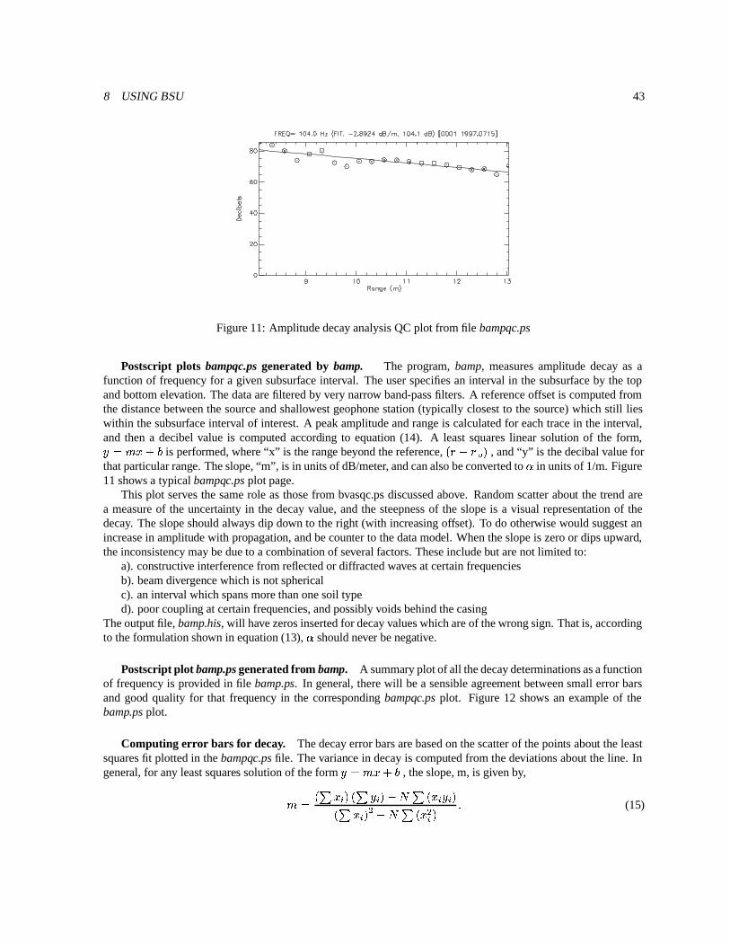
8 USING BSU 43

Figure 11: Amplitude decay analysis QC plot from file bampqc.ps

Postscript plots bampqc.ps generated by bamp. The program, bamp, measures amplitude decay as afunction of frequency for a given subsurface interval. The user specifies an interval in the subsurface by the topand bottom elevation. The data are filtered by very narrow band-pass filters. A reference offset is computed fromthe distance between the source and shallowest geophone station (typically closest to the source) which still lieswithin the subsurface interval of interest. A peak amplitude and range is calculated for each trace in the interval,and then a decibel value is computed according to equation (14). A least squares linear solution of the form,� � � � � � is performed, where “x” is the range beyond the reference,

" - " � & , and “y” is the decibal value forthat particular range. The slope, “m”, is in units of dB/meter, and can also be converted to

.in units of 1/m. Figure

11 shows a typical bampqc.ps plot page.This plot serves the same role as those from bvasqc.ps discussed above. Random scatter about the trend are

a measure of the uncertainty in the decay value, and the steepness of the slope is a visual representation of thedecay. The slope should always dip down to the right (with increasing offset). To do otherwise would suggest anincrease in amplitude with propagation, and be counter to the data model. When the slope is zero or dips upward,the inconsistency may be due to a combination of several factors. These include but are not limited to:

a). constructive interference from reflected or diffracted waves at certain frequenciesb). beam divergence which is not sphericalc). an interval which spans more than one soil typed). poor coupling at certain frequencies, and possibly voids behind the casing

The output file, bamp.his, will have zeros inserted for decay values which are of the wrong sign. That is, accordingto the formulation shown in equation (13),

.should never be negative.

Postscript plot bamp.ps generated from bamp. A summary plot of all the decay determinations as a functionof frequency is provided in file bamp.ps. In general, there will be a sensible agreement between small error barsand good quality for that frequency in the corresponding bampqc.ps plot. Figure 12 shows an example of thebamp.ps plot.

Computing error bars for decay. The decay error bars are based on the scatter of the points about the leastsquares fit plotted in the bampqc.ps file. The variance in decay is computed from the deviations about the line. Ingeneral, for any least squares solution of the form � � � � �� , the slope, m, is given by,

� � � � & � � & - � � J� � & � � & � -�� J� � & A (15)

8 USING BSU 44

Figure 12: Summary plot showing decay as a function of frequency

Here, N is the number of (x,y) pairs. We can estimate the variance in y from

� �� - � � �� &�& �� -�

A (16)

The variance in the slope, m, follows from the equation used to compute m, equation(15), and the variance in they values (which will be taken to be a constant given by equation(16)). For uncorrelated errors, the variance in theslope is given by

� �� < � �� ? � � �� # (17)

which reduces to the following

� �� "� � & - � � & � A (18)

The slope, m, for our problem is of course the decay factor (dB/m). Conversion to 1/m units follows by dividingby 8.68589 in the usual way.

8.1.15.4 Recording Aperture and the Selection of Filter Bandwidth for bvas and bamp As one might ex-pect, there is a limit to how finely the spectrum may be investigated. This depends on the available aperture, whichfollows from the choice the user made in recording the field data. If there are N samples in each seismic trace, andif the sample interval is

��, then the filter bandwidth should not be less than

�� . Further, the frequency step size(independent of the bandwidth specification) should be no smaller than the bandwidth. Both programs, bvas andbamp, should be run with the same spectral bandwidth. However, the program cainv3.sci is able to handle differenttotal numbers of amplitude and velocity samples in the frequency domain. Thus, it is OK to be missing eithersome decay or velocity samples. Further, the sampled frequencies do not have to be identical for both velocity anddecay. What should be the same is the bandwidth of the filters.

It is important to record enough data (large enough aperture), if the velocity measurements are to be consideredphase velocity, and not group velocity. With hammer sources on soil, I recommend recording no less than 0.5seconds of data (translates to a bandwidth of 2 Hz).

8 USING BSU 45

8.1.15.5 Inversion for Stiffness and Damping (cainv3.sci) Programs bvas and bamp store their results inbvas.his and bamp.his. The Scilab procedure, cainv3.sci, reads these files and performs the joint inversion for soilstiffness and damping. The procedure, caplot3.sci is available to produce journal quality plots of the inversionsolution. The Scilab procedures should be copied to the same directory where *.his files are located. Each depthinterval will require a separate set of *.his files, and a separate cainv3.sci run.

Start Scilab, and then from the Scilab text window, type the commandexec(’cainv3.sci’); Using a GUI interface, cainv3.sci will prompt you as follows:

DIALOG WITH CAINV3.SCI

1. Select input *.his file names. Default will work in most cases (click OK if bvas.his and bamp.his)

2. Select range of frequencies to invert. In the graphic display, move mouse to velocity panel and click withleft mouse button on the lowest frequency desired. Then move the mouse to the highest frequency desiredand click again.

3. Select starting point and number of iterations. The default is computed from equations (4) and (5). Thisis usually a good choice. But you can enter different values if you wish. The maximum number of iterationsis set to 10, and that is usually enough. See item (8) below.

4. Select weighting. Choose one of 3 options. The weighting reduces the influence of data points which havelarge uncertainties. One can weight by the reciprocal of the variance or the square root of the varianceestimate (stdv). If you want all data points to have an equal influence on the solution, regardless of theassociated measurement uncertainties, select the no weighting option.

5. Select data type balance point. This is a joint inversion which includes both velocity dispersion and decaymeasurements. A value near 1 will emphasize the velocity data, and largely ignore the decay information.A small value will emphasize the decay data, and discount the velocity information. Usually, one shouldrefrain from extremes here (don’t use 1 or 0), but stay in the range of 0.9 to 0.1 for useful results. Thisweighting is superimposed on a data type weighting (the least squares error has to be scaled to take intoaccount the different data units). If unsure, use the default, 0.5, for generally equal weighting of velocity anddecay.

6. Click on graphic window. Depending on your window manager, the iterations may flash the fit on thescreen, or require you to click the mouse at each iteration. With FVWM (the old one) you have to click.With most new window managers you can just watch, and hopefully things will converge on a solution.

7. Click on Continue. The procedure halts to let you view the last iteration results. When ready to move on,click on the YES button.

8. Click on Continue. View the weighted least squares error (this is a scaled combination error of both datatypes). It should decrease with iteration number, and give you an evaluation of the number of iterationsneeded. When ready to move on, click on the YES button.

9. Click on Continue. Chi-Square plots for velocity and decay are shown. These are based on averageestimates of the data uncertainties as expressed in the average error bars. It gives you an idea of the relativebalance between the residual error and the data uncertainty. In general, there is no point in obtaining asolution with Chi-square less than unity. More iterations may help if Chi-square is above unity, and can befurther reduced. However, if one only focuses on one data type, the other will suffer. See Menke [5] formore. When ready to move on, click on the YES button.

8 USING BSU 46

8.1.16 Plotting Inversion Results (caplot3.sci)

While the graphics produced during a cainv3.sci run are informative, you may wish to produce cleaner plots for apublication or document. Further, you may wish to draft on the figures using Xfig. A number of files are written bycainv3.sci which capture the solution and data from the inversion. These files are, casol.dat, caoutc.dat, caouta.dat,calsqe.dat, cadeld.dat, and cachi2.dat. These files are automatically read by caplot3.sci for a user specified plottingof the results.

From the Scilab text window, type the commandexec(’caplot3.sci’); Using a GUI interface, caplot3.sci will prompt you as follows:

DIALOG WITH CAPLOT3.SCI

1. Select confidence limits, error bars. Assuming normally distributed random error, select either 68% or95%.

2. Select grid. The plots will either have a blank background (NO) or a green grid (YES).

3. Set horizontal and vertical axis limits for Velocity Plot. The defaults are for everything. However, youmay want to focus on a portion of the data. Edit limits in the GUI and click OK.

4. Select range of observations to plot. During the inversion, you selected a subset of the frequencies thatcould be inverted. Do you want your final plot to show all the data, or just the range of frequencies youselected in the inversion? Click on ALL if you want to show all the data, regardless of whether or not it wasused in the solution. Click on FIT ONLY if you only want to include data that contributed to the solution.

5. Select axes length in inches. The output file will be in Xfig format, and the scaling assumes that intermediatestep (running Xfig, and then writing to a Postscript file from Xfig). Click on OK when ready. The procedurewill automatically write an Xfig file, cplot.fig. Typical Xfig editing will include rotating the Y-axis label.

6. Continue on to Decay Plot? Click YES to continue.

7. Set horizontal and vertical axis limits for Decay Plot. The defaults are for everything. However, you maywant to focus on a portion of the data. Edit limits in the GUI and click OK.

8. Select axes length in inches. The output file will be in Xfig format, and the scaling assumes that intermediatestep (running Xfig, and then writing to a Postscript file from Xfig). Click on OK when ready. The procedurewill automatically write an Xfig file, aplot.fig. Typical Xfig editing will include rotating the Y-axis label.

9. Continue to Chi-Square Plot? Click YES to continue.

10. Select axes limits. Defaults are usually OK. Click OK when ready to continue.

11. Select axes length in inches.

12. Mouse click to write Chi-Square labels. These labels are the average error bars for velocity and decay.You can take this opportunity to place them next to the respective curves. The first click is for velocity (solidcurve) and the second click is for attenuation (dashed curve). The procedure will automatically write an Xfigfile, chi2plot.fig.

8.1.16.1 Post caplot3.sci processing. You will want to edit the plot files in Xfig. At a minimum, you may wishto rotate the vertical axis label, and use the move button to adjust the placement of some labels, or perhaps the editbutton to modify the title of the plots. You can also merge two plots together, and even re scale the combination.Once you have it looking the way you wish, export the plot to a Postscript file for plotting or inclusion in adocument. An example with both velocity and decay merged together is shown in Figure 13.

8 USING BSU 47

0 10 20 30 40 50 60 70 80 90 1001101201301401500

100

200

300

.

⊕⊕⊕⊕

⊕⊕⊕⊕⊕⊕⊕⊕⊕⊕

⊕⊕⊕

⊕

⊕

⊕⊕⊕⊕⊕⊕⊕⊕⊕⊕⊕⊕

⊕⊕⊕

⊕⊕⊕⊕⊕⊕⊕⊕⊕⊕⊕⊕⊕⊕⊕⊕⊕⊕⊕⊕⊕⊕⊕⊕⊕⊕

Vel

ocity

(m

/s)

95% Conf. 1/Var error weighting Balance=0.50

Velocity C1=52139 (+/-)473 C2=20 (+/-)2

Frequency (Hz)

0 10 20 30 40 50 60 70 80 90 1001101201301401500.0

0.1

0.2

0.3

0.4

0.5

0.6

0.7

0.8

0.9

1.0

1.1

1.2

.⊕⊕⊕

⊕⊕⊕⊕⊕⊕⊕⊕⊕⊕⊕⊕⊕⊕

⊕

⊕⊕⊕⊕

⊕⊕⊕⊕⊕⊕⊕⊕

⊕⊕

⊕

⊕

⊕⊕⊕⊕⊕⊕⊕⊕

⊕⊕⊕⊕⊕⊕⊕

⊕⊕⊕⊕

⊕

⊕⊕⊕⊕⊕⊕Atte

nuat

ion

(1/m

)

95% Conf. 1/Var error weighting Balance=0.50

Attenuation C1=52139 (+/-)473 C2=20 (+/-)2

Frequency (Hz)

Figure 13: Merged figure showing both velocity and decay

8 USING BSU 48

8.2 Seismic Refraction Processing

The BSU package includes some software for the refraction delay time method. This software is suitable for asimple problem like mapping the depth to bedrock with a soil overburden. Engineering applications include slopestability analysis, assessment for the need to blast or excavate in construction, and mapping the extent of a soildeposit (like a gravel barrow). There are no assumptions about the recording surface, or the layout of the geophonesand shots. The ground topography can be irregular, and geophones do not always need to be deployed in a line.The seismic source can be buried, or on the surface of the ground.

This section will be illustrated with a data sample recorded along a highway where the issue was slope stability(Michaels [8] ). The Idaho Transportation Department was considering adding a passing lane, and the amount ofoverburden in the up dip direction was of concern. The sample file may be downloaded from the BSU web page,and is in refraction.tar.gz (419Kb).

8.2.1 The Refraction Data

Figure 14 is a base map showing a portion of the survey area. Data acquisition included a long line (5 metergeophone spacings) with reverse profiles along the shoulder of the highway. Shorter, cross lines were shot in theupslope direction with nominally 1 meter geophone spacings. The narrow right-of-way and steep slope conditionsprevented locating source points up the slope, and provided a severe restraint on the geophone locations in the zoneof most interest. A concern was that not enough offset could be obtained in the up-slope direction.

The problem was solved in two stages. First, we did conventional reverse profile interpretations of the longer,line which paralleled the roadway. Second, we used the first solution to constrain the delay time at source pointsused to acquire the cross-lines. In this example, we will work with just one of the cross-lines, line number 3. Wewill use two Bison records which were acquired with a hammer (15 fold vertical stack). In Figure 14 we see line1 (along the roadway) and the cross-line (line 3).

The source point for shot record 10 was located near station 24 on line 1. The source point for shot record 11was located near station 1 on line 1. The line 1 solution yielded a delay time of 0.0089 seconds at the hammerlocation for shot 10, and a delay time of 0.0150 seconds for the hammer location for shot 11. These values willbe used to constrain the line 3 solution. The other major constraint will be the refractor velocity, V2=4187 m/sdetermined from reverse profiles on line 1. This constraint is necessary since reverse profiles were not possible forline 3. As can be seen on Figure 14, the hammer blows fired broadside into line 3. The location for the source wasnot arbitrary, but chosen to be far enough away from all the geophone stations on line 3 (beyond the cross-overdistance for the refraction). The bedrock refractor was granite, the overburden was silty sand with gravel (Unifiedclassification SM). Soil testing indicated an internal angle of friction of � � A�� . Given that the topographic slopewas about � � � , the in place overburden was judged to be at the angle of repose.

8.2.2 Converting the Bison File to BSEGY, Setting Geometry (topcon, bis2seg, bhed)

If you have untarred the sample data set, you will find 3 files in the PREFIX/refraction/bison directory. The di-rectory, PREFIX, is where you were when you untarred the sample data archive. The files in the bison subdirectoryare:

� line3.nez [survey data from a Topcon total station, converted to NEZ format (5A12).

� bnk00010 [the Bison Engineering Seismograph file for shot 10]

� bnk00011 [the Bison Engineering Seismograph file for shot 11]

� gogeom [a script which will automate the process and is described next]

8 USING BSU 49

Figure 14: Base map for refraction survey (line 3 goes up hill from the roadway)

8 USING BSU 50

0

0.05

0.10

0.15

Tim

e (s

)

10 20 30 40Station

Scaled by 0.02532636 bsclk011.seg

pick

Figure 15: Scaled k011.seg refraction data

8.2.2.1 Contents of the gogeom script. The topcon man page and online documentation will be useful inunderstanding the first command. What it does is combine the survey information from line3.nez with headerinformation from the Bison file, bnk00010 to form a file, bnk00010.xyz which can be read by program bhed. Theprogram bis2seg converts the Bison file to a BSEGY file with minimal headers, then bhed is run and merges thebnk0010.xyz information into the headers to complete the geometry setting. The Unix move command, “mv” , isused in places to rename the file to the 4 character BSEGY convention. The flow is replicated for shot 11. Thegogeom script is as follows:

#!/bin/sh# convert Bison to BSEGY# shot10 (at station 24 line 1) Hammer Sourcetopcon line3.nez bnk00010 0003 0. 24 48 1 48 10 0. 0 180 0 0bis2seg bnk00010mv bnk00010.seg k010.segbhed k010.seg bnk00010.xyz 0mv bhedk010.seg k010.seg

# shot11 (at station 1 line 1) Hammer Sourcetopcon line3.nez bnk00011 0003 0. 1 48 1 48 11 0. 0 180 0 0bis2seg bnk00011mv bnk00011.seg k011.segbhed k011.seg bnk00011.xyz 0mv bhedk011.seg k011.seg

After running gogeom, you will have files k010.seg and k011.seg in the bison directory. Move these to thePREFIX/refraction/seg directory, and change to that directory for the next step in the process. Figure 15 is a plotof the k011.seg data. The data have been scaled by program bscl, and then plotted with Seismic Unix, clip=1.

8 USING BSU 51

1st break pick

Trace 11, k011.seg

0 0.01 0.02 0.03 0.04 0.05 0.06 0.07 0.08 0.09 0.10

-180

-140

-100

-60

-20

20

60

100

140

seconds

microvolts

Figure 16: Trace 11 as seen in segpic.sci run

By the way, for those who don’t have Bison formatted data, there is an alternative program in BSU namedtopcon2. It does essentially the same thing as topcon, but for SEG-2 formated seismograph files. You will need toread the man pages on topcon2, since there are some differences.

8.2.3 Picking First Breaks

This topic was initially covered in the down-hole section 8.1.13. As described in that section, one copies the filesegpic.sci into the working directory, starts Scilab and picks first arrivals. The program, bpic, is used to insert thepick times into the trace headers. Not all traces can be picked due to some background noise. In those cases,one should set the pick time to exactly zero, since program bref will use that convention to build suggestedconstraint equations. Figure 16 shows trace 11 of k011.seg as it appears during the execution of segpic.sci inScilab. My picks are included in the data sample distribution as files k010.pic and k011.pic for comparison withyour own picks.

8.2.4 Building the System of Delay Time Equations ( bref )

The philosophy behind program bref is that the computer does computations, but the user makes the decisions.The delay time formulation is described more fully in Michaels [6] . The formulation is a linear matrix equationof the form � � � $ #

(19)

where the matrix, G, contains information about the source and receiver geometry, m, is a vector of delay timesand the refractor slowness, and the vector, d, holds the observed first arrival pick times. When multiplied out, arow of equation (19) can be written as � � � �

� � �� #(20)

where

� � is a shot delay time,

�� is a geophone delay time, �� is the horizontal shot to geophone separation divided

by the refractor velocity, and��

is the first break pick time, assuming that the geophone is located far enough awayfrom the source to have the refracted head wave arrive before any other waves.

8 USING BSU 52

8.2.4.1 Running bref This is an interactive program which prompts the user as the following dialog illustrates.The user responses are boxed.

enter: line number (4 characters)0003Enter: number of shots2Enter: minimum offset to include40Enter: maximum offset to include200Is output for refraction or direct analysis?0=refraction 1=direct0irecip 0=normal 1=reciprocal shooting0Enter: input file namek010.segEnter: input file namek011.segshot x,y= 9927. 9773.shot x,y= 9883. 9666.Traces Processed = 48====> output in G0003====> listing in brefk010.lst

In the above example, the program writes 3 files, the last 4 characters of which are the line number as specifiedin the dialog.

1. G0003 system matrix, G, of equation (19)

2. D0003 data vector, d, of equation(19)

3. E0003 elevation file (3 columns; trace#, station_name, elevation)

In general, you will have to edit the Gxxxx and Dxxxx files. The sample data set (refraction.tar.gz) includesexamples of these files as created by bref (G0003.org etc.) and as modified to produce a constrained solution(G0003.mod etc.). The specific files created by bref will be highly dependent on the first break picks in the *.segfile trace headers. The convention is to flag picks exactly equal to zero as being unable to be picked. If none ofthe *.seg files has a pick at a particular geophone station, then the problem will be singular (unless you manuallyedit the file and add some rows to constrain the solution). Bref will make an attempt to add constraint rows to thebottom of the Gxxxx file, but they will be incomplete, since the user must decide what to do (don’t expect this codeto make critical decisions, that is your job).

8.2.4.2 Conventions: Structure of Gxxxx matrix The convention is to have the first N_shots columns corre-spond to source positions. The remaining N_traces columns correspond to the geophone stations. In our problem,there are 2 shot records, so the first two columns of G0003 are for shots 10 and 11 (because that was the orderthey were specified when running bref ). The remaining columns correspond to geophone stations in the order the

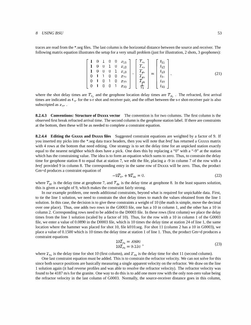
8 USING BSU 53

traces are read from the *.seg files. The last column is the horizontal distance between the source and receiver. Thefollowing matrix equation illustrates the setup for a very small problem (just for illustration, 2 shots, 3 geophones):��

�

� � � � � � %� � � � � � ��

� �� %��

� �%�

��1

��

� � ��

��

��

� %� �� %�� %�

��#

(21)

where the shot delay times are

� � and the geophone location delay times are

�� . The refracted, first arrival

times are indicated as� � � for the s-r shot and receiver pair, and the offset between the s-r shot-receiver pair is also

subscripted as� � � .

8.2.4.3 Conventions: Structure of Dxxxx vector The convention is for two columns. The first column is theobserved first break refracted arrival time. The second column is the geophone station label. If there are constraintsat the bottom, then these will be as needed to complete a constraint equation.

8.2.4.4 Editing the Gxxxx and Dxxxx files Suggested constraint equations are weighted by a factor of 9. Ifyou inserted my picks into the *.seg data trace headers, then you will note that bref has returned a Gxxxx matrixwith 4 rows at the bottom that need editing. One strategy is to set the delay time for an unpicked station exactlyequal to the nearest neighbor which does have a pick. One does this by replacing a “0” with a “-9” at the stationwhich has the constraining value. The idea is to form an equation which sums to zero. Thus, to constrain the delaytime for geophone station 8 to equal that at station 7, we edit the file, placing a -9 in column 7 of the row with abref provided 9 in column 8. The corresponding entry in the same row of Dxxxx will be zero. Thus, the productGm=d produces a constraint equation of - � � ��

�� A (22)

where

�� is the delay time at geophone 7, and

�� is the delay time at geophone 8. In the least squares solution,

this is given a weight of 9, which makes the constraint fairly strong.In our example problem, one needs additional constraints, beyond what is required for unpickable data. First,

to tie the line 1 solution, we need to constrain the shot delay times to match the values obtained from the line 1solution. In this case, the decision is to give these constraints a weight of 10 (the math is simple, move the decimalover one place). Thus, one adds two rows in the G0003 file, one has a 10 in column 1, and the other has a 10 incolumn 2. Corresponding rows need to be added to the D0003 file. In these rows (first column) we place the delaytimes from the line 1 solution (scaled by a factor of 10). Thus, for the row with a 10 in column 1 of the G0003file, we enter a value of 0.0890 in the D0003 file, which is 10 times the delay time at station 24 of line 1, the samelocation where the hammer was placed for shot 10, file k010.seg. For shot 11 (column 2 has a 10 in G0003), weplace a value of 0.1500 which is 10 times the delay time at station 1 of line 1. Thus, the product Gm=d produces aconstraint equations

� �� A � � ��

� �� A � � �

#(23)

where

� � � is the delay time for shot 10 (first column), and

� � � is the delay time for shot 11 (second column).One last constraint equation must be added. This is to constrain the refractor velocity. We can not solve for this

since both source positions are basically measuring a single apparent velocity on the refractor. We draw on the line1 solution again (it had reverse profiles and was able to resolve the refractor velocity). The refractor velocity wasfound to be 4187 m/s for the granite. One way to do this is to add one more row with the only non-zero value beingthe refractor velocity in the last column of G0003. Normally, the source-receiver distance goes in this column,

8 USING BSU 54

but here, we make it a constraint by adding a last row to D0003, and inserting a “data” value of 1.000 in the firstcolumn. Thus, the product GM=d produces a constraint equation

� �� A �� (24)

from this last row. The files G0003.mod, D0003.mod and E0003.mod included with the data sample are modifiedas described above.

8.2.5 Running the Delay Time Inversion (delaytm.sci and delaytmplot.sci)

The actual solution is computed in a Scilab procedure, delaytm.sci, found in the BSU distribution. The overburdenvelocity was determined to be 664 m/s from near offset and up hole analysis (line 1 was recorded with buriedexplosives). The procedure writes a number of *.dat files which are read by the plotting procedure, delaytmplot.sci.

Dialog when running delaytm.sci A number of GUI prompts require responses from the user. These aredescribed as follows:

� Choose a G matrix file. Select G0003.mod, or perhaps your own edited version. Click OK

� Choose a D vector file. Select D0003.mod, or your own version. Click OK.

� Choose an E vector file. Select E0003.mod, or your own version. Click OK.

� Number of Shots? Enter 2 and click OK.

� Number of Channels? Enter 48 and click OK.

� Enter smoothness constraint. Enter a value of 0.1. What this does is increase the least squares error slightly,but adds a built in change to the objective function (the spatial derivative of the delay time solution). A valueof zero here will produce the smallest error in the solution, but may map picking noise into false structure).

� The text window will show the shot delay times. They should agree with those specified in the constraintequations.

� The graphic window will have the refractor velocity in the title, and it should agree with the constraintapplied in our problem. The plotted curve is a graph of the delay time solution, geophones.

� Enter overburden velocity. Here, type in a value of 664 as discussed above.

� The graphic will show a plot of the ground topography and the refractor structure. This is one end-limitsolution that resolves the delay times completely as variations in the refractor structure. This is the preferredsolution for this geologic setting.

� Enter a constant refractor depth. This is an alternative solution which resolves the delay times as variationsin the overburden velocity (perhaps due to variations in water content). If you use the default, 10 m, you willsee that the overburden velocity would have to vary from 1265 to 300 m/s to explain the data. This end-limitsolution is not preferred in this geologic setting.

� Number of constraint equations? Enter 7 here, corresponding to the number of rows at the bottom of theG0003 file that we edited. This helps avoid a completely trashed plot where constraints become overprintedwith the time plot. With more than one shot record, there may be some over plot of the computed times inthis last graphic. You can fix that in Xfig, when you run delaytmplot.sci.

8 USING BSU 55

Resolving Delay Times The delaytm.sci procedure solves for the delay times, and then resolves them intotwo end-limit solutions. Variations in delay times are resolved totally into a variation in the refractor structure withthe formula � � � �� 1 � �� 235� � � � �� #

(25)

where

� � is the j-th delay time and “h” is the distance from the source or geophone to the refractor. This distance,h, is a radius specifying a circle, somewhere on which the refractor may be found. In delaytm.sci, the refractorposition is plotted a distance, h, directly below the source or geophone (unmigrated position). For the purpose ofmost engineering surveys, migration of the refractor point is not a significant issue (the distances are quite small).

The alternative end-limit resolution of delay times is as a variation in overburden velocity. The user provides adistance from the recording surface to the refractor (held constant), and an overburden velocity is found from theformula � /� � ��

� � �� # (26)

where

� � is the j-th delay time and “h” is the constant distance from the recording surface to the refractor. Thisassumes that the refractor velocity,

� � , is constant, and the only variation is in� , the overburden velocity. This

type of solution makes sense when the water content of the overburden soil is known to vary, and the overburdenthickness is relatively constant. In reality, the truth will be somewhere between these two limiting cases. SeeMichaels [6] for a discussion on this topic.

Running delaytmplot.sci is straight forward, and requires the sclplot.sci function be present in the workingdirectory. One should probably produce Xfig scaled plots, as some CAD work is usually required to clean thingsup. Figure 17 shows how a final merging of the exported *.fig files will look with a little CAD effort.

The default font is Times-Roman in Xfig. I have used a script, fixfig (see the BSU distribution script directory)which converts the fonts to Helvetica in a single sed (stream editor) pass. Simply type, fixfig foobar.ps to fix upa plot exported as Postscript from the Xfig program. Of course, you would substitute your particular postscript filename for foobar.ps.

8 USING BSU 56

Constrained Solution: k010.seg and k011.seg

V1=664 m/s

V2=4187 m/s granite

sandy silt

Picked Times Calculated Times from constrained solution

ground level

0 4 8 12 16 20 24 28 32 36 40 44 48980

985

990

995

1000

1005

1010

1015

1020

1025

1030

Station

Ele

vatio

n (m

)

0 4 8 12 16 20 24 28 32 36 40 44 4830

35

40

45

50

55

60

65

70

75

80

⊕ ⊕⊕⊕

⊕

⊕

⊕⊕⊕⊕⊕⊕⊕⊕⊕⊕⊕

⊕⊕⊕⊕⊕⊕⊕

⊕

⊕⊕⊕⊕⊕⊕⊕⊕

⊕⊕⊕⊕⊕

⊕⊕⊕

⊕⊕⊕⊕⊕⊕⊕

⊕ ⊕⊕⊕⊕⊕⊕⊕⊕

⊕⊕⊕⊕⊕⊕⊕

⊕⊕⊕⊕

⊕⊕⊕⊕⊕⊕⊕⊕⊕⊕

⊕⊕⊕⊕

⊕⊕

Pic

ks (

ms)

Station

⊕

Figure 17: Line 3 solution, merged Xfig plots produced by delaytmplot.sci

8 USING BSU 57

Horizontal Motion

away

P

SV

clip

up

down

Vertical Motion

P

SVR

Sign Convention NOT SEG Poisson’s Ratio = 1/4

R

(A) (B)

Solution to Lamb’s Problem(After Mooney, 1974)

clip

inward

0.4 0.6 0.8 1.0 1.2 1.4Normalized Time (Vs*t)/r

Dis

plac

emen

t

-0.2

-0.4

0.0

0.2

0.4

0.6

0.8

0.4 0.6 0.8 1.0 1.2 1.4Normalized Time (Vs*t)/r

Dis

plac

emen

t -1.2

-0.8

-1.0

0.0

-0.6

-0.4

-0.2

0.2

Figure 18: Solution to Lamb’s Problem (after Mooney, 1974). Step function source.

8.3 Solution to Lamb’s Problem (lamb)

The BSU distribution includes some synthetic seismogram capabilities. The solution of Lamb’s problem (Lamb[4] ) is computed by lamb. The program, lamb, is a recreation of a program originally described by Mooney [10] .The algorithm closely follows that described in Mooney’s paper, with the exception that an autoregressive operatoris used to generate a minimum phase wavelet to filter the data (Mooney convolved with a zero phase wavelet).Mooney’s work cites an earlier solution as the basis for his program (Pekeris [11] ), and that paper is well worthexamining for clarification on any points not entirely clear in Mooney’s publication. The current BSU version onlyimplements the case for a Poisson’s ratio of � . Modification to other cases is relatively straight forward, and willprobably be done at some point in the future.

Briefly, Lamb’s problem is the solution for the inhomogeneous waves that travel on the surface of an elastichalf-space due to a vertical, point impact source. Lamb referred to these waves as major and minor tremors. Today,we would call these the Rayleigh (major), P- and S-waves (minor). A test of the lamb program was to recreatepreviously published solutions plotted in unit less time. The unit less time coordinate is given by

� � � � 13��

#(27)

where R is the range (m) from the source, t is time (s), and� � is the shear wave velocity (m/s). This solution is

shown in Figure 18, and compares favorably with previously published solutions (Mooney [10] figure2; Pekeris[11] figures 3 and 4; and Richards [13] figures 2 and 3, integrals � � and � � respectively). The GSL library providesthe necessary elliptical integrals.

8.3.1 Running Program lamb

This program has 14 input arguments. The user is encouraged to review the man page and the online documentationfor lamb. For the man page, type man lamb . The online help is obtained by lamb -h .

8 USING BSU 58

Most arguments are straight forward, and obviously necessary to computing a synthetic seismogram. Since thecode only permits a Poisson’s ratio of � , the program only asks for a S-wave velocity,

� � . No P-wave velocity

can be entered since this limitation sets�� . The input argument, itype, is used to select what type of signal

will be output.

8.3.1.1 The itype argument in lamb.

� itype=1: The vertical and horizontal ground displacement will be computed and output in files lambv.segand lambh.seg, respectively. The source function is a displacement step function.

� itype=2: This may be viewed in either of two ways. The derivative of a step function is an impulse function,and itype=2 is the derivative with respect to time of the itype=1 case. Thus, this may be viewed as the grounddisplacement for an impulse source function. Alternatively, this can also be viewed as the ground particlevelocity for a source step function.

� itype=3: The source function is a single degree of freedom dampened resonator (exponentially decayingsinusoid wavelet, ground displacement function). The source is described by the sfreq and sdamp parameters.The output signals are ground displacements.

� itype=4: The source function is the same as itype=3, but the signals have been differentiated with respect totime. Thus, the output signals may be viewed as ground particle velocity for the itype=3 source.

� itype=5: This option switches the output signal from the actual ground motion to the motion of a geophoneelement (which is modeled as a single degree of freedom dampened oscillator bonded to the half-space atthe surface). The geophone is described by the gfreq and gdamp parameters.

� itype=6: The itype=5 option with the output signal differentiated with respect to time. The output is thegeophone element velocity. This case corresponds to the voltage that would be recorded by a velocitygeophone.

� itype=7: The output signal is the source displacement function corresponding to itype=3, at the point ofsource application. If you have run a case with itype=3, this is the source wavelet.

� itype=8: The particle velocity of the source function at the point of application. This corresponds to itype=4source wavelet.

� itype=9: This is like itype=7, with a geophone bonded at the source point. This is the displacement sourcewavelet as seen from the motion of a modeled geophone element.

� itype=10: This is like itype=8, with a geophone bonded at the source point. This is the particle velocity ofthe source wavelet as seen from the particle velocity of a geophone element bonded to the source point.

8.3.1.2 The pol argument in lamb. This selects a sign convention. In addition, if pol=0 (Test Mode), then the1/R amplitude decay is also removed (as was the case in computing Figure18). If pol=-1, then an upward motionproduces a negative value (the SEG sign convention). Setting pol=+1 reverses the sign convention (upward motionproduces a positive number). Interpreting pol for horizontal motion is much more confusing. In real life, one mustkeep track of the direction to the source, and the relative orientation of a geophone element, and how it is wired.Basically, if pol=0 or pol=+1, then the sign convention of the motion is as shown in Figure 18. If pol=-1, then itis the reverse of what is shown in Figure 18. In that figure, the word “away” means motion away from the sourcelocation (in the direction of increasing distance away from the source).

8 USING BSU 59

8.3.1.3 The stab argument in lamb. There really is no need for a stability factor, unless you are runningitype=8 which takes the derivative right at the source point, R=0. With all other itype values, you can set stab=0.The derivative operator used in lamb is a bilinear transform realization of the derivative with respect to time. Interms of the Z-transform,

� � & � �

�� 1 �- � & %

� �� & � � & 1�� & # (28)

where Y(z) is the output signal Z-transform, and X(z) is the input signal Z-transform. The stab factor nudges thepole at the Nyquist frequency slightly off the unit circle to prevent extreme blow up of any Nyquist amplitudes inthe input signal. The derivative is realized by an ARMA operator. The formula which realizes equation (28) is

� � � �� J� � - � �� &!- � ��

� �� & #

(29)

where � � is the j-th sample corresponding to the temporal derivative of� � , the j-th sample of the input signal being

differentiated.

8.3.1.4 Examples of lamb The signals shown in Figure 18 were computed by lamb in Test Mode (pol=0). Thecommand to generate the Figure 18 signals is

lamb 150. 1.0 1 2. .0005 150. 1700. 1 100. .3 100. .3 0 0.Not all of the parameters matter (density won’t affect the result since it is test mode). There are many com-

binations of S-wave velocity and range that will work (see equation (27) for normalized time scale used here).You can generate the plots of Figure 18 to confirm correct operation of the code. This is done in Scilab, executethe procedure seisplot.sci from within the Scilab text window. Make sure you also have the functions bsegin.sci,segyinfo.sci, and sclplot.sci in the working directory as they are called by seisplot.sci. Also note that you will haveto specify the axes limits to clip the signals as was done in Figure 18.

As a second example of what lamb can do, we can generate 48 channel records for vertical and inline radialmotion. The half-space medium has a mass density of 1700

� �� , a� � � � � � m/s and

� � � � � � m/s. The commandgenerating the synthetic seismograms is

lamb 1. 1.0 48 .5 .0005 250. 1700. 6 50. .7 10. .7 -1 0.Figure 19 shows the resulting synthetics. Note that this is an elastic medium assumption. Actual soils may

differ significantly from an elastic assumption. So, take it for what it is.

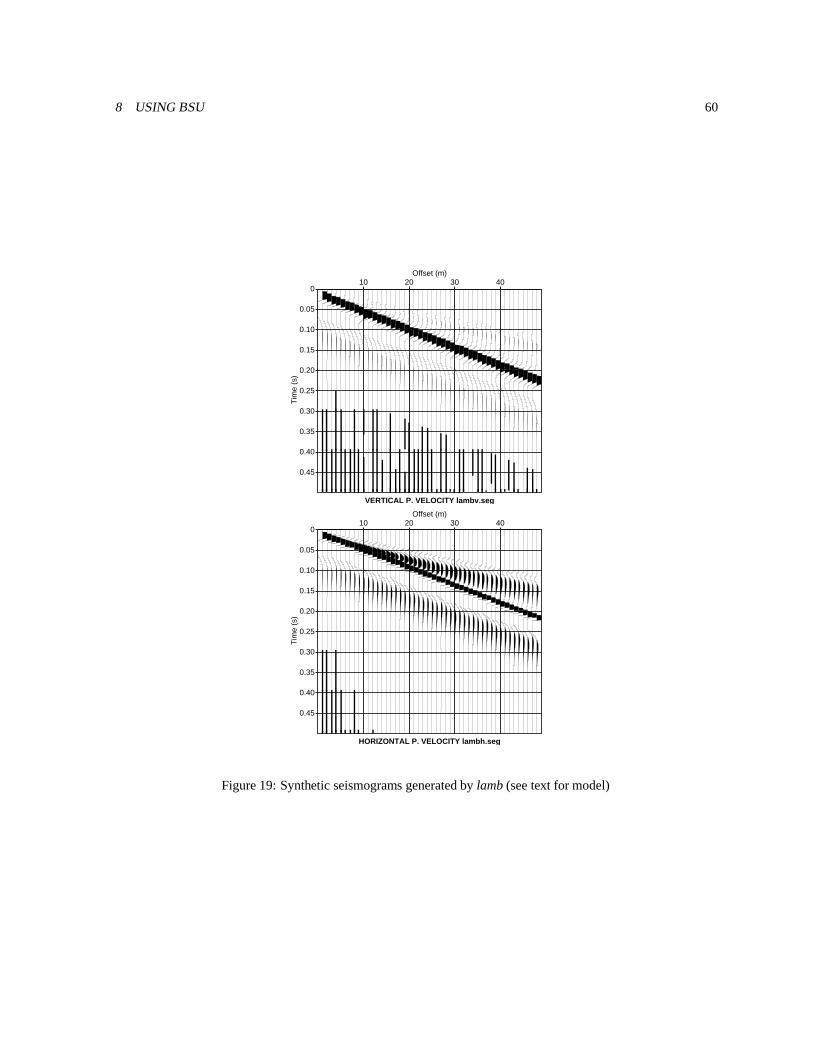
8 USING BSU 60

0

0.05

0.10

0.15

0.20

0.25

0.30

0.35

0.40

0.45

Tim

e (s

)

10 20 30 40Offset (m)

VERTICAL P. VELOCITY lambv.seg

0

0.05

0.10

0.15

0.20

0.25

0.30

0.35

0.40

0.45

Tim

e (s

)

10 20 30 40Offset (m)

HORIZONTAL P. VELOCITY lambh.seg

Figure 19: Synthetic seismograms generated by lamb (see text for model)

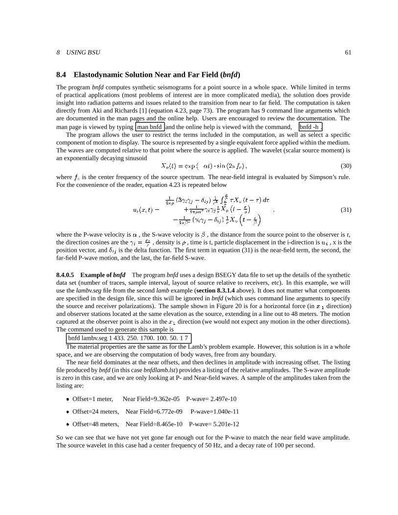
8 USING BSU 61

8.4 Elastodynamic Solution Near and Far Field (bnfd)

The program bnfd computes synthetic seismograms for a point source in a whole space. While limited in termsof practical applications (most problems of interest are in more complicated media), the solution does provideinsight into radiation patterns and issues related to the transition from near to far field. The computation is takendirectly from Aki and Richards [1] (equation 4.23, page 73). The program has 9 command line arguments whichare documented in the man pages and the online help. Users are encouraged to review the documentation. Theman page is viewed by typing man bnfd and the online help is viewed with the command, bnfd -h .

The program allows the user to restrict the terms included in the computation, as well as select a specificcomponent of motion to display. The source is represented by a single equivalent force applied within the medium.The waves are computed relative to that point where the source is applied. The wavelet (scalar source moment) isan exponentially decaying sinusoid �

� J�'& � (�*,+ �-/.0�'&!1�5� � �� M &�# (30)

where� M is the center frequency of the source spectrum. The near-field integral is evaluated by Simpson’s rule.

For the convenience of the reader, equation 4.23 is repeated below

� "�$#%�'& � �� - � & � �� "� - � & $ �� E � - �� H- �� -� � & � � �

� � - �� #

(31)

where the P-wave velocity is.

, the S-wave velocity is7

, the distance from the source point to the observer is r,the direction cosines are the � � � �� , density is � , time is t, particle displacement in the i-direction is

� , x is the

position vector, and � is the delta function. The first term in equation (31) is the near-field term, the second, the

far-field P-wave motion, and the last, the far-field S-wave.

8.4.0.5 Example of bnfd The program bnfd uses a design BSEGY data file to set up the details of the syntheticdata set (number of traces, sample interval, layout of source relative to receivers, etc). In this example, we willuse the lambv.seg file from the second lamb example (section 8.3.1.4 above). It does not matter what componentsare specified in the design file, since this will be ignored in bnfd (which uses command line arguments to specifythe source and receiver polarizations). The sample shown in Figure 20 is for a horizontal force (in

� direction)and observer stations located at the same elevation as the source, extending in a line out to 48 meters. The motioncaptured at the observer point is also in the

� direction (we would not expect any motion in the other directions).The command used to generate this sample is

bnfd lambv.seg 1 433. 250. 1700. 100. 50. 1 7The material properties are the same as for the Lamb’s problem example. However, this solution is in a whole

space, and we are observing the computation of body waves, free from any boundary.The near field dominates at the near offsets, and then declines in amplitude with increasing offset. The listing

file produced by bnfd (in this case bnfdlamb.lst) provides a listing of the relative amplitudes. The S-wave amplitudeis zero in this case, and we are only looking at P- and Near-field waves. A sample of the amplitudes taken from thelisting are:

� Offset=1 meter, Near Field=9.362e-05 P-wave= 2.497e-10

� Offset=24 meters, Near Field=6.772e-09 P-wave=1.040e-11

� Offset=48 meters, Near Field=8.465e-10 P-wave= 5.201e-12

So we can see that we have not yet gone far enough out for the P-wave to match the near field wave amplitude.The source wavelet in this case had a center frequency of 50 Hz, and a decay rate of 100 per second.

9 APPENDIX A (BHELP LISTING) 62

force observer

0

0.05

0.10

0.15

0.20

0.25

0.30

0.35

0.40

0.45

Tim

e (s

)

10 20 30 40Offset (m)

Motion in X1 Direction, Force in X1 Direction bnfdlamb.seg

Figure 20: Near and Far Field computations (source in x1, motion in x1 directions)

9 Appendix A (bhelp listing)

MAIN PROGRAMS:Directory=BSUROOT/C/bsegy/ or BSUROOT/Fort/bsegy/

babs.c rectify seismic tracesbagc.c automatic gain control of traces (scale in time and space)bamp.f amplitude analysis by frequency (Kelvin-Voigt solid)bbal.c balances two data sets to have same MAV (mean absolute value)bbox.c apply moving average (box car) filter as function of timebcad.f plot seismic traces as CAD (*.dxf; digital exchange file)bcnv.c FORMAT CONVERSION: BSEGY <---> SEG-Y (BSU=*.seg, SEG-Y=*.sgy)bcrd.f coordinate rotation and translation, BSEGY geometry headersbdat.c datuming program for refraction data (easier for picking)bdcn.f deconvolution (profile or trace mode), prediction or error outbdif.f differentiates w.r.t. time using Bilinear Transform methodbdum.f generate dummy data set with user defined impulse positionbdump.f generate a dump of selected BSEGY header valuesbedt.f edit BSEGY seismic file (traces, time, sample interval, etc.)bequ.c trace equalize data by L2 norm or Maximum Absolute Valuebext.c extract traces from a merged data set based on header valuesbfil.f ARMA FILTER of seismic traces (low-, band-, or high-pass)bftr.f FILTER traces with other *.seg traces, or namelist from bdumpbfxt.f F-X Transform of seismic tracesbgar.c exponential GAIN recovery, by range specification


bgaz.c exponential GAIN recovery, by depth specificationbhed.f up/down load selected header information from/to a text filebhelp.c this listing of BSU package contentsbhod.f hodogram by PCA to determine down-hole tool orientationbint.f numerical integration of seismic traces (trapezoidal rule)bis2seg.c FORMAT CONVERSION: BISON ---> BSEGY (no geometry setting)bkil.f either kill (delete) or zero seismic tracesbmed.f median mix of seismic traces (spatial)bmix.f mean mix of seismic traces (spatial)bmrg.f merge traces from many files to a single filebmrk.f mark first break picks with a delta function on waveformbmst.f MASTER illustrates programing in BSU, FORTRANbnfd.c MODELING: computes near and far field in elastic whole spacebnos.f MODELING: generate band-limited random noise tracesboff.c computed source to receiver offset and add to headersbpic.f automatic first break picker, or inserts picks from a filebrdc.f remove DC bias from tracesbred.f apply linear or hyperbolic correction in time to tracesbref.f delay time refraction analysis setupbrev.f reverse either channel order or sample polaritybrot.f rotate seismic traces (3-component data)brsp.f resample data in time (augmentation with zeros in freq domain)bscl.f scale data set with user provided, or data derived factorbsdc.f show DC level in seismic traces as %MAV (mean absolute value)bshf.f apply a static shift to seismic traces (shift in time)bshp.f Wiener least squares shaping filterbsrt.c sorts traces by offsetbstk.f stacks traces in a gather (number traces out=number in)bsum.c weighted sum of two data sets: file_out = file1 + C*file2btor.f applies geophone orientations to trace headers (from PCA)bvas.f measures body wave velocity dispersion (Kelvin-Voigt solid)bvax.f measures velocity dispersion on surface databvel.f apply correctional velocity (linear with range)bvsp.f down-hole travel time inversion with ray bendingbwht.f non-linear whitening program (agc applied to bank of filters)bwin.f window the data aperture with raised cosine tapersbxcr.f cross (or auto) correlation, output to BSEGY data setcaplot.f PostScript plots of combined bvas and bamp runscmst.c MASTER illustrates programing in BSU, C-LANGUAGEegg2seg.c FORMAT CONVERSION: EEG’s SEG-2 ---> BSEGY (no geometry)genb2s.f BASH SCRIPT GENERATOR: sets up a block of bis2seg runsgenbhod.f BASH SCRIPT GENERATOR: sets up for PCA analysis s-wave sourcegenbhodV.f BASH SCRIPT GENERATOR: sets up for PCA analysis vert. sourcegenbrot.f BASH SCRIPT GENERATOR: sets up for run of brot on many filesgenref.f BASH SCRIPT GENERATOR: for geometry setting on pattern, CDPgensetg.c generates control files for geometry setting, setgeom programgenvsp.f BASH SCRIPT GENERATOR: setting geometry for down-hole surveysgplt.c plots seismic traces to a GIF file (uses PBMPLUS Toolkit)


lamb.c MODELING: computes solution to Lamb’s problem (Vp/Vs=sqrt(3))seg2txt.f FORMAT CONVERSION: BSEGY ----> ASCII (for Scilab or Matlab)setgeom.c Sets geometry for reciprocal refraction shooting (see gensetg)top2dxf.f FORMAT CONVERSION: Survey NEZ (*.nez) ---> CAD (*.dxf)top2nez.f FORMAT CONVERSION: RAW TOPCON ---> Survey NEZ (*.nez)topbcrd.f apply coordinate translation and rotation to Survey NEZ (*.nez)topcon.f combines NEZ with BISON file --->*.xyz file Run bhed on *.xyztopcon2.c combines NEZ with EGG SEG-2 ---> BSEGY with geometrytraplt.f line printer style plots of samples and spectrum

C-FUNCTIONS: Directory=BSUROOT/C/sublib4/bargrid.c draw a progress bar grid to screen (stdout)c_boxit.c apply a running average (box car) filter to a signalc_bsegin.c read a seismic trace in BSEGY formatc_bsegout.c write a seismic trace in BSEGY formatcr_labl.c write a copyright label to screen (stdout)exbar.c draw progress bar to screen (stdout)fcr_labl.c write a copyright label to a filefindxyz.c extract geophone and source coordinates from headersfmax_min.c compute maximum and minimum value in a signal, and indexesfnorm.c compute L2 norm of a signalhlp_labl.c print a help label to screen (stdout)in_chk.c scan a data set for number of traces, sample interval, etc.lsqufit.c least squares fit, straight line function: y=mx + bmav.c compute mean absolute value of a signalnames.c build file names from process IDonepole.c perform a single pole (Z-plane) filter

FORTRAN SUBROUTINES: Directory=BSUROOT/Fort/sublib4/agc.f apply Automatic Gain Control (AGC) on a signalarma.f apply an Autoregressive Moving Average (ARMA) filterbnoise.f compute band-limited random noiseboxit.f apply a running average (box car) filter to a signalbsegin.f read a seismic trace in BSEGY formatbsegout.f write a seismic trace in BSEGY formatcfilt.f design a bank of band-pass digital filterschktrc.f scan a data set for number of traces, sample interval, etc.conv.f apply a selected filter out of bank designed by cfilt.fconv2.f time domain convolution of two signalscross.f E. A. Robinson’s cross correlation subroutinecshift.f shift traces in frequency domain by phase rotationczero.f zero a complex signaldemult.f demultiplex a complex trace into real and imag. partsdot.f E. A. Robinson’s inner (dot) product between two vectorsdrum.f E. A. Robinson’s phase unwrapping subroutine (modified by pm)eureka.f E. A. Robinson’s solution by Levinson Recursionfindxyz.f extract geophone and source coordinates from headersflist.f line printer style plot of a complex signal (spectrum)


fmed.f bubble sort on a vector, returns median valuefold.f E. A. Robinson’s convolution subroutinel2norm.f rescale a seismic signal by its L2 normnlogn.f E. A. Robinson’s Fast Fourier Transform (Radix 2)nrad2.f determines the first power of two larger than a given valuepltbar.f draw progress bar to screen (like bargrid.c and exbar.c)polar.f E. A. Robinson’s conversion from rectangular to polar formrand.f CMLIB: generates uniform pseudo-random numberrect.f convert complex numbers from polar to rectangular formrunif.f CMLIB: calls rand.f to generate longer period random sequenceshape.f E. A. Robinson’s least squares shaping filtertlist.f line printer style plot of a signal (also lists values)vshft.f shifts a signal by linear interpolation of samplesxcor.f cross correlates two signalsxcor1.f one sided autocorrelation of a signalxmax.f find maximum and minimum values in a vector

C-INCLUDE FILES: Directory=BSUROOT/C/include/c_bsegy.h BSEGY header structuresub4.h prototypes of library functionspbm.h BBMPLUS Toolkit used in gplt.cpbmplus.hpgm.hppm.hppmcmap.h

Directory=BSUROOT/C/gsleval.h Extracted from GNU Scientific Library (GSL)error.h (see comment below)config.h

Directory=BSUROOT/C/gsl/gsl/gsl_errno.h Extracted from GNU Scientific Library (GSL)gsl_math.h These are needed for the elliptical integralsgsl_precision.h in lamb.c, and are provided for those who have notgsl_sf_ellint.h yet installed GSL on their system. If you don’tgsl_message.h have GSL, you might want to install it if you aregsl_machine.h a scientist or engineer who writes C code.gsl_sys.hgsl_nan.h The source code for the elliptical integrals cangsl_pow_int.h be found in BSUROOT/C/sublib4, and are compiledgsl_mode.h into that static library. They are:gsl_sf_result.h ellint.c infnan.c error.c fdiv.c prec.c stream.c

FORTRAN INCLUDE FILES: Directory=BSUROOT/C/includebsegy.inc BSEGY header declaration and equivalence statements


LIBRARIES:BSUROOT/Fort/sublib4/sublib4.aBSUROOT/C/sublib4/sublib4.aBSUROOT/C/pbmplus/pbmlib.a PBMPLUS Toolkit (gplt.c)

PLPLOT: Assume you have installed it as follows:/usr/local/plplot/lib/libplplot.so.5.1.0 shared (make file uses this/usr/local/plplot/lib/libplplot.a bvas.c bamp.c)

Scilab: Directory=BSUROOT/Scilabsegpic.sci Pick first breaks (Seismic Unix has some better tools)seisplot.sci Plot seismic tracesseishodo.sci Plot hodogramwiggleplot.sci Plot tracesdelaytm.sci Delaytime analysisdelaytmplot.sci Plot delay time analysis resultsseginfo.sci Scan a BSEGY filebsegin.sci Reads seismic traces in BSEGY formatsclplot.sci Make a plot with axes scaled for paper sizetraplt.sci Plot a signal from a BSEGY data set

10 APPENDIX B (MERGE-ALL) 67

10 Appendix B (Merge-all)

The following bash script is used in down-hole surveys to form the various resorted data sets. These include bothdifference and sum of opposite source polarizations, for each individual component.

#!/bin/sh# Merge-all: basic script to merge traces in all combinations# (sum or difference) by each component.## Notation: component/location/sum or dif/# Examples:# tddf=Tcomponent, down-hole, difference# trdf=Tcomponent, reference, difference# tdsm=Tcomponent, down-hole, sum# trsm=Tcomponent, reference, sum## This combines all the shot gathers into receiver gathers for the differ-

ent# geophone components in a down-hole survey. You should have run bhod first# to determine tool orientation, btor to insert orientations into headers,

# and brot to rotate the data into a standard orientation. If you have, then# you can run this script.## Copyright (c) 2002 Paul Michaels# <[email protected]># This program is free software; you can# redistribute it and/or modify it under the terms# of the GNU General Public License as published# by the Free Software Foundation; either version# 2 of the License, or (at your option) any later# version. This program is distributed in the# hope that it will be useful, but# WITHOUT ANY WARRANTY; without even the implied# warranty of MERCHANTABILITY or FITNESS FOR A# PARTICULAR PURPOSE. See the GNU General Public# License for more details.# You should have received a copy of the GNU# General Public License along with this program;# if not, write to the Free Software Foundation,# Inc., 675 Mass Ave, Cambridge, MA 02139, USA.

#set -x

#...define parameters YOU MUST DEFINE THESE FOR EACH NEW SURVEY# SINCE IT IS LIKELY THAT THE NUMBER OF RECORDS# WILL VARY WITH EACH SURVEY !!!!odmin=01odmax=145


evmin=02evmax=146PRFX=L# eklmax=(odmax-1)/2eklmax=‘bc <<END

($odmax-1)/2END‘echo $eklmax# oklmax=eklmax+1oklmax=‘bc <<END

($eklmax+1)END‘echo $oklmax

#shaping filter parameters (bshp)tmin=0.tmax=0.1npf=360stab=.0001

#polarity file definitionsaz90=1az270=2

#Scale Data by VERTICAL REF (ch4) (Absolute Scale from last, evmax)bscl brot$PRFX$evmax.seg 4 1 3 1>/dev/nullAMP=‘gawk ’/Peak Absolute Value/ {print $4}’ bsclbrot.lst‘echo $AMP

FILE=‘find brot*seg | sed s/\.seg/”/g |sed s/brot/”/g‘for i in $FILE; do

bscl brot$i.seg 4 1 3 1>/dev/nullmv bsclbrot.seg bscl$i.segbscl bscl$i.seg 4 1 0 $AMP 1>/dev/nullmv bsclbscl.seg bscl$i.seg

done

#...reference phone gathers (VERTICAL=ch4)bmrg bscl$PRFX $odmin $odmax 2 4 4 1>/dev/nullmv bmrg.seg rfv1.segbmrg bscl$PRFX $evmin $evmax 2 4 4 1>/dev/nullmv bmrg.seg rfv2.seg

#...reference phone gathers (RADIAL=ch5)bmrg bscl$PRFX $odmin $odmax 2 5 5 1>/dev/nullmv bmrg.seg rfr1.segbmrg bscl$PRFX $evmin $evmax 2 5 5 1>/dev/nullmv bmrg.seg rfr2.seg


#...reference phone gathers (TRANSVERSE=ch6)bmrg bscl$PRFX $odmin $odmax 2 6 6 1>/dev/nullmv bmrg.seg rft1.segbmrg bscl$PRFX $evmin $evmax 2 6 6 1>/dev/nullmv bmrg.seg rft2.seg

#...down hole swc phone gathers (TRANSVERSE=ch3)bmrg bscl$PRFX $odmin $odmax 2 3 3 1>/dev/nullmv bmrg.seg swt1.segbmrg bscl$PRFX $evmin $evmax 2 3 3 1>/dev/nullmv bmrg.seg swt2.seg

#...down hole swc phone gathers (RADIAL=ch2)bmrg bscl$PRFX $odmin $odmax 2 2 2 1>/dev/nullmv bmrg.seg swr1.segbmrg bscl$PRFX $evmin $evmax 2 2 2 1>/dev/nullmv bmrg.seg swr2.seg

#...down hole swc phone gathers (VERTICAL=ch1)bmrg bscl$PRFX $odmin $odmax 2 1 1 1>/dev/nullmv bmrg.seg swv1.segbmrg bscl$PRFX $evmin $evmax 2 1 1 1>/dev/nullmv bmrg.seg swv2.seg#---------------------------------------------

# Notation: component/location/sum or dif/# tddf=Tcomponent, down-hole, difference# trdf=Tcomponent, reference, difference# tdsm=Tcomponent, down-hole, sum# trsm=Tcomponent, reference, sum##DIFFERENCE ENHANCEMENT# downhole (side wall clamping phone)bsum swt$az90.seg swt$az270.seg -1.0mv bsumswt$az90.seg tddf.seg

bsum swv$az90.seg swv$az270.seg -1.0mv bsumswv$az90.seg vddf.seg

bsum swr$az90.seg swr$az270.seg -1.0mv bsumswr$az90.seg rddf.seg

# reference phone at surfacebsum rft$az90.seg rft$az270.seg -1.0mv bsumrft$az90.seg trdf.seg

bsum rfr$az90.seg rfr$az270.seg -1.0


mv bsumrfr$az90.seg rrdf.seg

bsum rfv$az90.seg rfv$az270.seg -1.0mv bsumrfv$az90.seg vrdf.seg#---------------------------------------------

#SUM ENHANCEMENT# downhole (side wall clamping phone)bsum swt$az90.seg swt$az270.seg +1.0mv bsumswt$az90.seg tdsm.seg

bsum swv$az90.seg swv$az270.seg +1.0mv bsumswv$az90.seg vdsm.seg

bsum swr$az90.seg swr$az270.seg +1.0mv bsumswr$az90.seg rdsm.seg

# reference phone at surfacebsum rft$az90.seg rft$az270.seg +1.0mv bsumrft$az90.seg trsm.seg

bsum rfr$az90.seg rfr$az270.seg +1.0mv bsumrfr$az90.seg rrsm.seg

bsum rfv$az90.seg rfv$az270.seg +1.0mv bsumrfv$az90.seg vrsm.seg

#---------------------------------------------#make links to alias names like Mergeln -s tddf.seg twav.segln -s trdf.seg tref.segln -s vdsm.seg pwav.segln -s vrsm.seg vref.seg

#SH-WAVE SHAPING#...take last trace as a targetbkil trdf.seg 1 1 1 $eklmax 1>/dev/nullbstk bkiltrdf.seg 1>/dev/nullbscl bstkbkil.seg 1 1 0 $oklmax.0 1>/dev/nullmv bsclbstk.seg targ.seg

#...determine shaping filters and apply to T-Reference rft*.segbshp trdf.seg targ.seg 1 1 $tmin $tmax $npf $stab#...apply shaping filters to downhole T-data swt*.segbshp trdf.seg targ.seg 1 0 $tmin $tmax $npf $stab tddf.segmv bshptddf.seg twave.seg#---------------------------------------------


#P-WAVE SHAPING#...take last trace as a targetbkil vrsm.seg 1 1 1 $eklmax 1>/dev/nullbstk bkilvrsm.seg 1>/dev/nullbscl bstkbkil.seg 1 1 0 $oklmax.0 1>/dev/nullmv bsclbstk.seg varg.seg

#...determine shaping filters and apply to T-Reference rfv*.segbshp vrsm.seg varg.seg 1 1 $tmin $tmax $npf $stab#...apply shaping filters to downhole T-data swv*.segbshp vrsm.seg varg.seg 1 0 $tmin $tmax $npf $stab vdsm.segmv bshpvdsm.seg pwave.seg#---------------------------------------------

#...quick view of resultsbequ twave.seg 0 .25gplt bequtwav.seg 0 .25 1 100 2. 1 5mv plot.gif twave.gifxv twave.gif

#...quick view of resultsbequ pwave.seg 0 .025gplt bequpwav.seg 0 .05 1 100 2. 1 5mv plot.gif pwave.gifxv pwave.gif

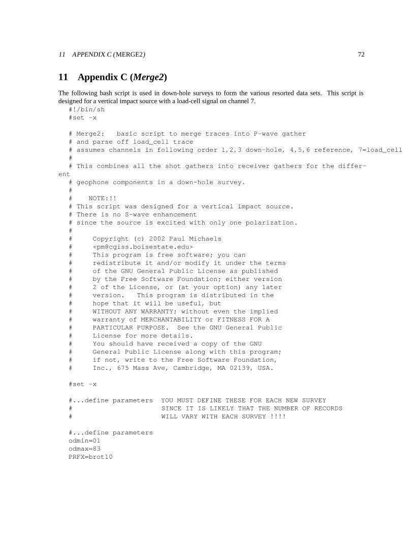
11 APPENDIX C (MERGE2) 72

11 Appendix C (Merge2)

The following bash script is used in down-hole surveys to form the various resorted data sets. This script isdesigned for a vertical impact source with a load-cell signal on channel 7.

#!/bin/sh#set -x

# Merge2: basic script to merge traces into P-wave gather# and parse off load_cell trace# assumes channels in following order 1,2,3 down-hole, 4,5,6 reference, 7=load_cell## This combines all the shot gathers into receiver gathers for the differ-

ent# geophone components in a down-hole survey.## NOTE:!!# This script was designed for a vertical impact source.# There is no S-wave enhancement# since the source is excited with only one polarization.## Copyright (c) 2002 Paul Michaels# <[email protected]># This program is free software; you can# redistribute it and/or modify it under the terms# of the GNU General Public License as published# by the Free Software Foundation; either version# 2 of the License, or (at your option) any later# version. This program is distributed in the# hope that it will be useful, but# WITHOUT ANY WARRANTY; without even the implied# warranty of MERCHANTABILITY or FITNESS FOR A# PARTICULAR PURPOSE. See the GNU General Public# License for more details.# You should have received a copy of the GNU# General Public License along with this program;# if not, write to the Free Software Foundation,# Inc., 675 Mass Ave, Cambridge, MA 02139, USA.

#set -x

#...define parameters YOU MUST DEFINE THESE FOR EACH NEW SURVEY# SINCE IT IS LIKELY THAT THE NUMBER OF RECORDS# WILL VARY WITH EACH SURVEY !!!!

#...define parametersodmin=01odmax=83PRFX=brot10

11 APPENDIX C (MERGE2) 73

#pull off load_cell channelsbmrg $PRFX $odmin $odmax 1 7 7 1>/dev/nullmv bmrg.seg ldcl.segecho "created ldcl.seg (load cell traces)"

#pull off vertical reference phonebmrg $PRFX $odmin $odmax 1 4 4 1>/dev/nullmv bmrg.seg refv.segecho "created refv.seg (vertical reference traces) "

#pull off radial reference phonebmrg $PRFX $odmin $odmax 1 5 5 1>/dev/nullmv bmrg.seg refr.segecho "created refr.seg (radial reference traces) "

#pull off transverse reference phonebmrg $PRFX $odmin $odmax 1 6 6 1>/dev/nullmv bmrg.seg reft.segecho "created reft.seg (transverse reference traces)"

#pull off vertical down-hole phonebmrg $PRFX $odmin $odmax 1 1 1 1>/dev/nullmv bmrg.seg swcv.segecho "created swcv.seg (vertical swc phone traces) "

#pull off radial down-hole phonebmrg $PRFX $odmin $odmax 1 2 2 1>/dev/nullmv bmrg.seg swcr.segecho "created swcr.seg (radial swc phone traces) "

#pull off transverse down-hole phonebmrg $PRFX $odmin $odmax 1 3 3 1>/dev/nullmv bmrg.seg swct.segecho "created swct.seg (transverse swc phone traces)"echo done

12 GNU GENERAL PUBLIC LICENSE VERSION 2, JUNE 1991 74

12 GNU GENERAL PUBLIC LICENSE Version 2, June 1991

Copyright (C) 1989, 1991 Free Software Foundation, Inc. 59 Temple Place, Suite 330, Boston, MA 02111-1307USA Everyone is permitted to copy and distribute verbatim copies of this license document, but changing it is notallowed.

Preamble

The licenses for most software are designed to take away your freedom to share and change it. By contrast, theGNU General Public License is intended to guarantee your freedom to share and change free software–to make surethe software is free for all its users. This General Public License applies to most of the Free Software Foundation’ssoftware and to any other program whose authors commit to using it. (Some other Free Software Foundationsoftware is covered by the GNU Library General Public License instead.) You can apply it to your programs, too.

When we speak of free software, we are referring to freedom, not price. Our General Public Licenses aredesigned to make sure that you have the freedom to distribute copies of free software (and charge for this service ifyou wish), that you receive source code or can get it if you want it, that you can change the software or use piecesof it in new free programs; and that you know you can do these things.

To protect your rights, we need to make restrictions that forbid anyone to deny you these rights or to ask youto surrender the rights. These restrictions translate to certain responsibilities for you if you distribute copies of thesoftware, or if you modify it.

For example, if you distribute copies of such a program, whether gratis or for a fee, you must give the recipientsall the rights that you have. You must make sure that they, too, receive or can get the source code. And you mustshow them these terms so they know their rights.

We protect your rights with two steps: (1) copyright the software, and (2) offer you this license which givesyou legal permission to copy, distribute and/or modify the software.

Also, for each author’s protection and ours, we want to make certain that everyone understands that there is nowarranty for this free software. If the software is modified by someone else and passed on, we want its recipientsto know that what they have is not the original, so that any problems introduced by others will not reflect on theoriginal authors’ reputations.

Finally, any free program is threatened constantly by software patents. We wish to avoid the danger thatredistributors of a free program will individually obtain patent licenses, in effect making the program proprietary.To prevent this, we have made it clear that any patent must be licensed for everyone’s free use or not licensed atall.

The precise terms and conditions for copying, distribution and modification follow.

GNU GENERAL PUBLIC LICENSE TERMS AND CONDITIONS FOR COPYING,DISTRIBUTION AND MODIFICATION

0. This License applies to any program or other work which contains a notice placed by the copyright holdersaying it may be distributed under the terms of this General Public License. The "Program", below, refers toany such program or work, and a "work based on the Program" means either the Program or any derivative workunder copyright law: that is to say, a work containing the Program or a portion of it, either verbatim or withmodifications and/or translated into another language. (Hereinafter, translation is included without limitation inthe term "modification".) Each licensee is addressed as "you".

Activities other than copying, distribution and modification are not covered by this License; they are outsideits scope. The act of running the Program is not restricted, and the output from the Program is covered only ifits contents constitute a work based on the Program (independent of having been made by running the Program).Whether that is true depends on what the Program does.


1. You may copy and distribute verbatim copies of the Program’s source code as you receive it, in any medium,provided that you conspicuously and appropriately publish on each copy an appropriate copyright notice anddisclaimer of warranty; keep intact all the notices that refer to this License and to the absence of any warranty; andgive any other recipients of the Program a copy of this License along with the Program.

You may charge a fee for the physical act of transferring a copy, and you may at your option offer warrantyprotection in exchange for a fee.

2. You may modify your copy or copies of the Program or any portion of it, thus forming a work based on theProgram, and copy and distribute such modifications or work under the terms of Section 1 above, provided thatyou also meet all of these conditions:

a) You must cause the modified files to carry prominent notices stating that you changed the files and the dateof any change.

b) You must cause any work that you distribute or publish, that in whole or in part contains or is derived fromthe Program or any part thereof, to be licensed as a whole at no charge to all third parties under the terms of thisLicense.

c) If the modified program normally reads commands interactively when run, you must cause it, when startedrunning for such interactive use in the most ordinary way, to print or display an announcement including anappropriate copyright notice and a notice that there is no warranty (or else, saying that you provide a warranty)and that users may redistribute the program under these conditions, and telling the user how to view a copy of thisLicense. (Exception: if the Program itself is interactive but does not normally print such an announcement, yourwork based on the Program is not required to print an announcement.) These requirements apply to the modifiedwork as a whole. If identifiable sections of that work are not derived from the Program, and can be reasonablyconsidered independent and separate works in themselves, then this License, and its terms, do not apply to thosesections when you distribute them as separate works. But when you distribute the same sections as part of a wholewhich is a work based on the Program, the distribution of the whole must be on the terms of this License, whosepermissions for other licensees extend to the entire whole, and thus to each and every part regardless of who wroteit.

Thus, it is not the intent of this section to claim rights or contest your rights to work written entirely by you;rather, the intent is to exercise the right to control the distribution of derivative or collective works based on theProgram.

In addition, mere aggregation of another work not based on the Program with the Program (or with a workbased on the Program) on a volume of a storage or distribution medium does not bring the other work under thescope of this License.

3. You may copy and distribute the Program (or a work based on it, under Section 2) in object code orexecutable form under the terms of Sections 1 and 2 above provided that you also do one of the following:

a) Accompany it with the complete corresponding machine-readable source code, which must be distributedunder the terms of Sections 1 and 2 above on a medium customarily used for software interchange; or,

b) Accompany it with a written offer, valid for at least three years, to give any third party, for a charge no morethan your cost of physically performing source distribution, a complete machine-readable copy of the correspond-ing source code, to be distributed under the terms of Sections 1 and 2 above on a medium customarily used forsoftware interchange; or,

c) Accompany it with the information you received as to the offer to distribute corresponding source code.(This alternative is allowed only for noncommercial distribution and only if you received the program in objectcode or executable form with such an offer, in accord with Subsection b above.)

The source code for a work means the preferred form of the work for making modifications to it. For anexecutable work, complete source code means all the source code for all modules it contains, plus any associatedinterface definition files, plus the scripts used to control compilation and installation of the executable. However,as a special exception, the source code distributed need not include anything that is normally distributed (in eithersource or binary form) with the major components (compiler, kernel, and so on) of the operating system on which


the executable runs, unless that component itself accompanies the executable.If distribution of executable or object code is made by offering access to copy from a designated place, then

offering equivalent access to copy the source code from the same place counts as distribution of the source code,even though third parties are not compelled to copy the source along with the object code. 4. You may notcopy, modify, sublicense, or distribute the Program except as expressly provided under this License. Any attemptotherwise to copy, modify, sublicense or distribute the Program is void, and will automatically terminate yourrights under this License. However, parties who have received copies, or rights, from you under this License willnot have their licenses terminated so long as such parties remain in full compliance.

5. You are not required to accept this License, since you have not signed it. However, nothing else grantsyou permission to modify or distribute the Program or its derivative works. These actions are prohibited by lawif you do not accept this License. Therefore, by modifying or distributing the Program (or any work based onthe Program), you indicate your acceptance of this License to do so, and all its terms and conditions for copying,distributing or modifying the Program or works based on it.

6. Each time you redistribute the Program (or any work based on the Program), the recipient automaticallyreceives a license from the original licensor to copy, distribute or modify the Program subject to these terms andconditions. You may not impose any further restrictions on the recipients’ exercise of the rights granted herein.You are not responsible for enforcing compliance by third parties to this License.

7. If, as a consequence of a court judgment or allegation of patent infringement or for any other reason (notlimited to patent issues), conditions are imposed on you (whether by court order, agreement or otherwise) thatcontradict the conditions of this License, they do not excuse you from the conditions of this License. If you cannotdistribute so as to satisfy simultaneously your obligations under this License and any other pertinent obligations,then as a consequence you may not distribute the Program at all. For example, if a patent license would not permitroyalty-free redistribution of the Program by all those who receive copies directly or indirectly through you, thenthe only way you could satisfy both it and this License would be to refrain entirely from distribution of the Program.

If any portion of this section is held invalid or unenforceable under any particular circumstance, the balance ofthe section is intended to apply and the section as a whole is intended to apply in other circumstances.

It is not the purpose of this section to induce you to infringe any patents or other property right claims orto contest validity of any such claims; this section has the sole purpose of protecting the integrity of the freesoftware distribution system, which is implemented by public license practices. Many people have made generouscontributions to the wide range of software distributed through that system in reliance on consistent application ofthat system; it is up to the author/donor to decide if he or she is willing to distribute software through any othersystem and a licensee cannot impose that choice.

This section is intended to make thoroughly clear what is believed to be a consequence of the rest of thisLicense. 8. If the distribution and/or use of the Program is restricted in certain countries either by patents orby copyrighted interfaces, the original copyright holder who places the Program under this License may add anexplicit geographical distribution limitation excluding those countries, so that distribution is permitted only in oramong countries not thus excluded. In such case, this License incorporates the limitation as if written in the bodyof this License.

9. The Free Software Foundation may publish revised and/or new versions of the General Public License fromtime to time. Such new versions will be similar in spirit to the present version, but may differ in detail to addressnew problems or concerns.

Each version is given a distinguishing version number. If the Program specifies a version number of thisLicense which applies to it and "any later version", you have the option of following the terms and conditionseither of that version or of any later version published by the Free Software Foundation. If the Program doesnot specify a version number of this License, you may choose any version ever published by the Free SoftwareFoundation.

10. If you wish to incorporate parts of the Program into other free programs whose distribution conditionsare different, write to the author to ask for permission. For software which is copyrighted by the Free Software


Foundation, write to the Free Software Foundation; we sometimes make exceptions for this. Our decision will beguided by the two goals of preserving the free status of all derivatives of our free software and of promoting thesharing and reuse of software generally.

NO WARRANTY11. BECAUSE THE PROGRAM IS LICENSED FREE OF CHARGE, THERE IS NO WARRANTY FOR

THE PROGRAM, TO THE EXTENT PERMITTED BY APPLICABLE LAW. EXCEPT WHEN OTHERWISESTATED IN WRITING THE COPYRIGHT HOLDERS AND/OR OTHER PARTIES PROVIDE THE PROGRAM"AS IS" WITHOUT WARRANTY OF ANY KIND, EITHER EXPRESSED OR IMPLIED, INCLUDING, BUTNOT LIMITED TO, THE IMPLIED WARRANTIES OF MERCHANTABILITY AND FITNESS FOR A PAR-TICULAR PURPOSE. THE ENTIRE RISK AS TO THE QUALITY AND PERFORMANCE OF THE PRO-GRAM IS WITH YOU. SHOULD THE PROGRAM PROVE DEFECTIVE, YOU ASSUME THE COST OFALL NECESSARY SERVICING, REPAIR OR CORRECTION.

12. IN NO EVENT UNLESS REQUIRED BY APPLICABLE LAW OR AGREED TO IN WRITING WILLANY COPYRIGHT HOLDER, OR ANY OTHER PARTY WHO MAY MODIFY AND/OR REDISTRIBUTETHE PROGRAM AS PERMITTED ABOVE, BE LIABLE TO YOU FOR DAMAGES, INCLUDING ANY GEN-ERAL, SPECIAL, INCIDENTAL OR CONSEQUENTIAL DAMAGES ARISING OUT OF THE USE OR IN-ABILITY TO USE THE PROGRAM (INCLUDING BUT NOT LIMITED TO LOSS OF DATA OR DATA BEINGRENDERED INACCURATE OR LOSSES SUSTAINED BY YOU OR THIRD PARTIES OR A FAILURE OFTHE PROGRAM TO OPERATE WITH ANY OTHER PROGRAMS), EVEN IF SUCH HOLDER OR OTHERPARTY HAS BEEN ADVISED OF THE POSSIBILITY OF SUCH DAMAGES.

END OF TERMS AND CONDITIONS

How to Apply These Terms to Your New Programs

If you develop a new program, and you want it to be of the greatest possible use to the public, the best way toachieve this is to make it free software which everyone can redistribute and change under these terms.

To do so, attach the following notices to the program. It is safest to attach them to the start of each source fileto most effectively convey the exclusion of warranty; and each file should have at least the "copyright" line and apointer to where the full notice is found.

<one line to give the program’s name and a brief idea of what it does.> Copyright (C) 19yy <name of author>This program is free software; you can redistribute it and/or modify it under the terms of the GNU General

Public License as published by the Free Software Foundation; either version 2 of the License, or (at your option)any later version.

This program is distributed in the hope that it will be useful, but WITHOUT ANY WARRANTY; without eventhe implied warranty of MERCHANTABILITY or FITNESS FOR A PARTICULAR PURPOSE. See the GNUGeneral Public License for more details.

You should have received a copy of the GNU General Public License along with this program; if not, write tothe Free Software Foundation, Inc., 59 Temple Place, Suite 330, Boston, MA 02111-1307 USA

Also add information on how to contact you by electronic and paper mail.If the program is interactive, make it output a short notice like this when it starts in an interactive mode:Gnomovision version 69, Copyright (C) 19yy name of author Gnomovision comes with ABSOLUTELY NO

WARRANTY; for details type ‘show w’. This is free software, and you are welcome to redistribute it under certainconditions; type ‘show c’ for details.

The hypothetical commands ‘show w’ and ‘show c’ should show the appropriate parts of the General PublicLicense. Of course, the commands you use may be called something other than ‘show w’ and ‘show c’; they couldeven be mouse-clicks or menu items–whatever suits your program.

You should also get your employer (if you work as a programmer) or your school, if any, to sign a "copyrightdisclaimer" for the program, if necessary. Here is a sample; alter the names:


Yoyodyne, Inc., hereby disclaims all copyright interest in the program ‘Gnomovision’ (which makes passes atcompilers) written by James Hacker.

<signature of Ty Coon>, 1 April 1989 Ty Coon, President of ViceThis General Public License does not permit incorporating your program into proprietary programs. If your

program is a subroutine library, you may consider it more useful to permit linking proprietary applications withthe library. If this is what you want to do, use the GNU Library General Public License instead of this License.

13 REFERENCES 79

13 References

References

[1] K. Aki and P.G. Richards. Quantitative Seismology Vol. 1, volume 1. W.H. Freeman and Co., 1980. 557p.

[2] J. K. Cohen and Jr. J. W. Stockwell. CWP/SU: Seismic Unix release 34: a free package for seismic researchand processing. Center for Wave Phenomena, Colorado School of Mines, 2000.

[3] D. Crice. BHG-2, BHG-3 borehole geophone operation manual. GeoStuff, 19623 via Escuela Dr., Saratoga,Ca 95070, 1996. 16p.

[4] H. Lamb. On the propagation of tremors over the surface of an elastic solid. Phil. Tran. Royal Society ofLondon, Series A(203):1–42, 1904.

[5] W. Menke. Geophysical data analysis, discrete inverse theory. Academic Press, 1989. San Diego 289pgs.

[6] P. Michaels. A geophysical site investigation for a bridge foundation in a narrow canyon. Environmental &Engineering Geoscience, 1(2):219–226, 1995.

[7] P Michaels. In situ determination of soil stiffness and damping. Journal of Geotechnical and Geoenviron-mental Engineering, 24(8):709–719, 1998.

[8] P. Michaels. Use of engineering geophysics in the design of highway passing lanes. Proceedings of the Sym-posium on the Application of Geophysics to Engineering and Environmental Problems, SAGEEP99, pages179–187, 1999.

[9] P. Michaels. Use of principal component analysis to determine down-hole tool orientation and enhance SH-waves. Journal of Environmental and Engineering Geophysics, 6(4):175–183, 2001.

[10] H.M. Mooney. Some numerical solutions for Lamb’s problem. Bulletin of the Seismological Society ofAmerica, 64(2):473–491, 1974.

[11] C.L. Pekeris. The seismic surface pulse. Proceedings of the National Academy of Science, 41:469–480, 1955.

[12] W.H. Press, B.P. Flannery, S.A. Teukolsky, and W.T. Vetterling. Numerical Recipes, The art of scientificcomputing Fortran version. Cambridge University Press, 1989. 702p.

[13] P.G. Richards. Elementary solutions to Lamb ’s problem for a point source and their relevance to three-dimensional studies of spontaneous crack propagation. Bulletin of the Seismological Society of America,69(4):947–956, 1979.

[14] E.A. Robinson. Multichannel Time Series Analysis with Digital Computer Programs. Holden-Day, 1967.298p.

[15] R.E. Sheriff. Encyclopedic dictionary of exploration geophysics. Society of Exploration Geophysics, 1991.

14 Index

Indexbamp, 42bamp.ps, 43bampqc.ps, 43bdump, 30bhed, 25, 48bhelp, 18, 62bhod, 26bis2seg, 25, 48Bison, 48bnfd, 61bpic, 37bref, 51brot, 31bsegin.sci, 59btor, 28bvas, 40bvas.his, 40bvas.ps, 40bvasqc.ps, 40bvsp, 37

cainv3.sci, 40, 45caplot3.sci, 45, 46CMLIB, 8ConeTec, 37constraint equations, 53conventions, bref, 52conventions, naming, 15conventions, parameter, 15

damping, 39data sample, description, 23data sample, down-hole, 20delay time, 51delaytm.sci, 54delaytmplot.sci, 54, 55derivative, 59differential equation, 39divergence, spherical, 42documentation, BSU, 18

editing, bref files, 53editing, Merge, 32elastic, 57, 59elastodynamic, 61error bars, 46

error bars, decay, 43error bars, velocity, 42

far field, 61filter selection, 44fixfig, 55

genbhod, 26genbrot, 31genvsp, 23, 30geophone, down-hole, 20geophone, reference, 20GNU license, 2, 74gobhodo, 27gobhodoR, 27gogeom, 50gorunbhod, 27gorunbhodR, 27gplt, 34GSL, 8

Helvetica, 55hodogram, 27hodograms, 28

installing, BSU, 11installing, LAPACK, 10installing, PLPLOT, 9Inversion, stiffness and damping, 45itype, 58

lamb, 57Lamb’s Problem, 57LAPACK, 7locations, functions and subroutines, 18lst, 27, 28

man pages, 19Merge, 32Merge procedure, 33merge-all, 67Merge2, 72mergeplots, 27Merging, 32

near field, 61NEZ, 48

80

INDEX 81

obtaining BSU, 6

packages, optional, 8packages, required, 6PCA, 26, 28pdf, 27Picking, 36picking, first breaks, 51PLPLOT, 6programming, 14programming, C-language, 17programming, Fortran77, 16psPlot, 34

quality control, 40quality control, decay, 43quality control, picks, 37quality control, velocity, 40

recording aperture, 44refraction, 48rename-btor, 29

Scilab, 8, 51sclplot.sci, 55, 59SEG-2, 51segpic.sci, 36, 51segyinfo.sci, 59Seismic Unix, 9, 34, 50seisplot.sci, 59semblance, 40slope stability, 48Sorting, 32source, seismic, 20stiffness, 39

topcon, 48, 51topcon2, 51

user’s guide, 19

vertical time, 37vfitw.sci, 37vplot.sci, 37

Xfig, 9, 46, 55xPlot, 34

Z-transform, 59

basic seismic utilities user’s guide - lsu geology & … seismi… · · 2007-07-24basic...

Documents