balancing of the shaking force, shaking moment, input
TRANSCRIPT
Rochester Institute of Technology Rochester Institute of Technology
RIT Scholar Works RIT Scholar Works
Theses
1985
Balancing of the Shaking Force, Shaking Moment, Input Torque Balancing of the Shaking Force, Shaking Moment, Input Torque
and Bearing Forces in Planar Four Bar Linkages and Bearing Forces in Planar Four Bar Linkages
Timothy C. Hewitt
Follow this and additional works at: https://scholarworks.rit.edu/theses
Recommended Citation Recommended Citation Hewitt, Timothy C., "Balancing of the Shaking Force, Shaking Moment, Input Torque and Bearing Forces in Planar Four Bar Linkages" (1985). Thesis. Rochester Institute of Technology. Accessed from
This Thesis is brought to you for free and open access by RIT Scholar Works. It has been accepted for inclusion in Theses by an authorized administrator of RIT Scholar Works. For more information, please contact [email protected].
BALANCING OF THE SHAKING FORCE, SHAKING MOMENT, INPUT TORQUE
AND BEARING FORCES IN PLANAR FOUR BAR LINKAGES
Approved by
USING
AUTOMATED OPTIMAL DESIGN
by
Timothy C. Hewitt
A Thesis Submitted
in
Partial Fulfillment
of the
Requirements for the Degree of
MASTER OF SCIENCE
in
Mechanical Engineering
Prof. ~~(-=T"""'h-e-s---'i-s-A""Q.=-v""i'-,s""o-r-) --
Prof. ---------------Prof. --------------------Prof.
-T(EB=e~p~a~I;t;m~e~n~t~H~e~a~dT)--
DEPARTMENT OF MECHANICAL ENGINEERING
ROCHESTER INSTITUTE OF TECHNOLOGY
ROCHESTER, NEW YORK
January, 1985
To : Whom it may Concern
2472 Old State Route 32
Batavia, Ohio 45103
January 31, 1984
Regarding : Reproduction of thesis entitled" Balancing of
the Shaking Force, Shaking Moment, Input Torque,
and Bearing Forces in Planar Four Bar Linkages "
I, Timothy C. Hewitt, do hereby grant permission to the
Wallace Memorial Library to reproduce my thesis in whole, or
in part. It is my understanding that any reproduction will
not be for commercial use or profit.
Signed,
Timothy C. Hewitt
ACKNOWLEDGEMENTS
The author would like to take this opportunity to thank
all those who have assisted him throughout the development of
this thesis and in particular:
Dr. W. F. Halbleib, the author's thesis advisor, for
his patience, advice and direction throughout the course of
this thesis. In addition, for instilling the importance of
fundamental ideas in the author.
Dr. R. C. Johnson, member of the author's thesis
committee, whose efforts in the field of automated optimal
design have made a substantial portion of this thesis
possible.
Dr. P- Venkataraman, member of the author's thesis
committee, for his insight and suggestions concerning this
thesis.
Mr. L. Dearstyne of the Eastman Kodak Company,
Rochester, N.Y. for his insight and suggestions concerning
the initial development of the problem.
The Eastman Kodak Company, Rochester, N.Y. for
assistance and support of a computer aided literature search.

The College of Engineering of the Rochester Institute of
Technology, Rochester, N.Y. and the Aircraft Engine Business
Group of the General Electric Company, Evendale, O.H. for use
of their VAX/VMS 11/782 digital computers.
To the author's wife and family, for their continued
support and patience throughout the author's graduate program.
ABSTRACT
The theory, development and application of a computer
program to balance the combined effects of the shaking force,
shaking moment, input torque and individual bearing forces in
four bar linkages is presented. The theory assumes the
linkage to consist of rigid bodies, and is limited to
balancing planar four bar linkages other than sliders.
Balancing is accomplished using circular counterweights which
are tangentially attached to the bearing joints.
Counterweight sizes and locations are determined using
nonlinear programming techniques where an objective function,
dependent upon all the kinetic parameters, is minimized.
The balancing program is capable of performing diverse
functions. The number of added counterweights, type and
degree of numerical quadrature and regional constraints on all
important balancing parameters can be varied. In addition,
the program is capable of balancing linkages with offline mass
distributions, and to some extent, emphasis can be placed on
individual terms such as the input torque. A major limitation
of the theory is the assumption of rigid links. This may not
always be valid and makes the program insensitive to natural
frequencies, where the amount of vibration would be excessive-
Example problems are presented to show the capabilities
and application of the balancing program. The first example
shows the effect of varying the degree and type of numerical
integration used. The Gaussian quadrature method is shown to
be most efficient, with the optimum number of sampling points
determined to be 10. In example two, an inline four bar
linkage operating at a constant input speed of 5000 rpm is
balanced so that all kinetic quantities are reduced from 75%
to 92% over the unbalanced case. Similar results are shown in
example three for balancing a four bar linkage with an offline
coupler mass distribution. The effect of adding from one to
three counterweights is also investigated, with the results
indicating that additional counterweights do not always
improve the balancing situation. With just one counterweight
added, the important kinetic terms are reduced an average of
87%, while the addition of three counterweights only reduces
these same quantities an additional 5%.
Due to the apparent success of the developed program, the
author recommends that it be extended to sliders, six bars and
other practical linkages. In addition, the validity of the
rigid body assumption should be experimentally and
theoretically investigated.

TABLE OF CONTENTS
Page
i LIST OF FIGURES i
i i LIST OF TABLES iii
iv NOMENCLATURE v
1 . 0 INTRODUCTION 1
2 . 0 LITERATURE SURVEY 4
3 . 0 OVERVIEW OF THE THEORY 10
4.0 DEVELOPMENT OF THE KINEMATIC AND KINETIC EQUATIONS 13
4.1 Two Point Mass Model 13
4.2 Kinematic Analysis 22
4.3 Newtonian Approach 28
4.4 Lagrangian Approach 43
4.5 Combined Approach 52
5.0 DEVELOPMENT OF THE OPTIMIZATION PROBLEM AND GENERAL
BALANCING PROGRAM 63
5.1 Objective Function Proposal 63
5.2 Statement of the Optimization Problem 65
5.3 Summary of the AOD Program 69
5.4 Summary of the Analysis and Final Subroutines 75
6 . 0 PRESENTATION OF THE EXAMPLE PROBLEMS 80
6.1 Capabilities of the OPTBAL Computer Program 82
6.2 Balancing of an Inline Four Bar Linkage 93
6.3 Balancing of a Four Bar with an Offline Coupler
Link 97
7.0 DISCUSSION OF RESULTS 109
8.0 CONCLUSIONS 115
9.0 RECOMMENDATIONS 117
10.0 REFERENCES 118
11.0 APPENDIX A - PRINCIPLES OF ANGULAR MOMENTUM Al
12.0 APPENDIX B - SOLUTION OF THE TWO POINT MASS MODEL
CONVERSION BI
13 . 0 APPENDIX C - SUMMARY OF NUMERICAL INTEGRATION CI
14 . 0 APPENDIX D - COMPUTER PROGRAM OPTBAL Dl
LIST OF FIGURES
Figure Title Page
1 General Four Bar Linkage with Circular
Counterweights 14
2 Two Point Mass Model 14
3 Combined C. G. Location of a General Link
with a Circular Counterweight 17
4 Two Point Mass Model of a Combined C.G. Location 17
5 - Stick Figure of a Four Bar Linkage 23
6 Free Body Diagram of a General Two Point
Mass Model ^9
7 Free Body Diagram of a Two Point Mass Model
Separated from its Frame 53
8 Flowchart of the MODSER Program 72
9 Relationship between the AOD program and
Analysis, Final, and Pgauss Subroutines 76
10 Example 1 Inline Four Bar Linkage 83
11 Example 1 Normalized Rms Input Torque
Versus the Number of Sampling Points 85
12 Example 1 Normalized Rms Shaking Force
Versus the Number of Sampling Points 86
13 Example 1 Normalized Rms Shaking Moment
Versus the Number of Sampling Points 87
Page i
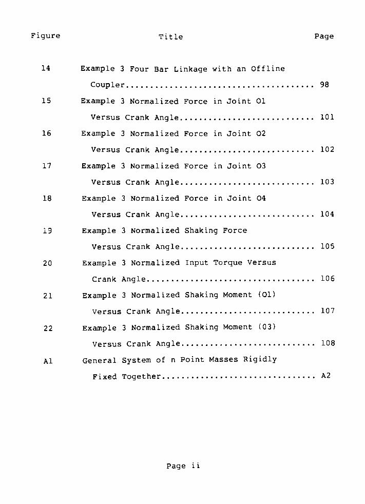
Figure Title Page
14 Example 3 Four Bar Linkage with an Offline
Coupler 98
15 Example 3 Normalized Force in Joint 01
Versus Crank Angle 101
16 Example 3 Normalized Force in Joint 02
Versus Crank Angle 102
17 Example 3 Normalized Force in Joint 03
Versus Crank Angle 103
18 Example 3 Normalized Force in Joint 04
Versus Crank Angle 104
19 Example 3 Normalized Shaking Force
Versus Crank Angle 105
20 Example 3 Normalized Input Torque Versus
Crank Angle 106
21 Example 3 Normalized Shaking Moment (01)
Versus Crank Angle 107
22 Example 3 Normalized Shaking Moment (03)
Versus Crank Angle 108
Al General System of n Point Masses Rigidly
Fixed Together A2
Page ii
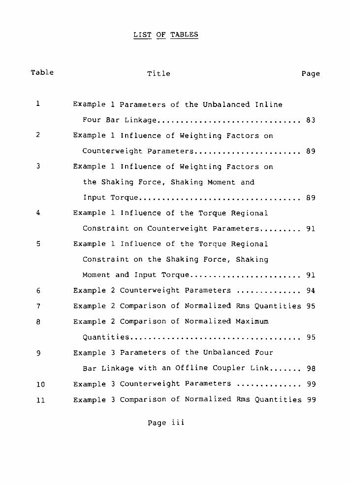
LIST OF TABLES
Table Title Page
1 Example 1 Parameters of the Unbalanced Inline
Four Bar Linkage 83
2 Example 1 Influence of Weighting Factors on
Counterweight Parameters 89
3 Example 1 Influence of Weighting Factors on
the Shaking Force, Shaking Moment and
Input Torque 89
4 Example 1 Influence of the Torque Regional
Constraint on Counterweight Parameters 91
5 Example 1 Influence of the Torque Regional
Constraint on the Shaking Force, Shaking
Moment and Input Torque 91
6 Example 2 Counterweight Parameters 94
7 Example 2 Comparison of Normalized Rms Quantities 95
8 Example 2 Comparison of Normalized Maximum
Quantities 95
9 Example 3 Parameters of the Unbalanced Four
Bar Linkage with an Offline Coupler Link 98
10 Example 3 Counterweight Parameters 99
11 Example 3 Comparison of Normalized Rms Quantities 99
Page iii

Table Title Page
Al Definitions of Angular Momentum A5
CI Abscissas and Weighting Factors for Gaussian
Integration C6
Page iv
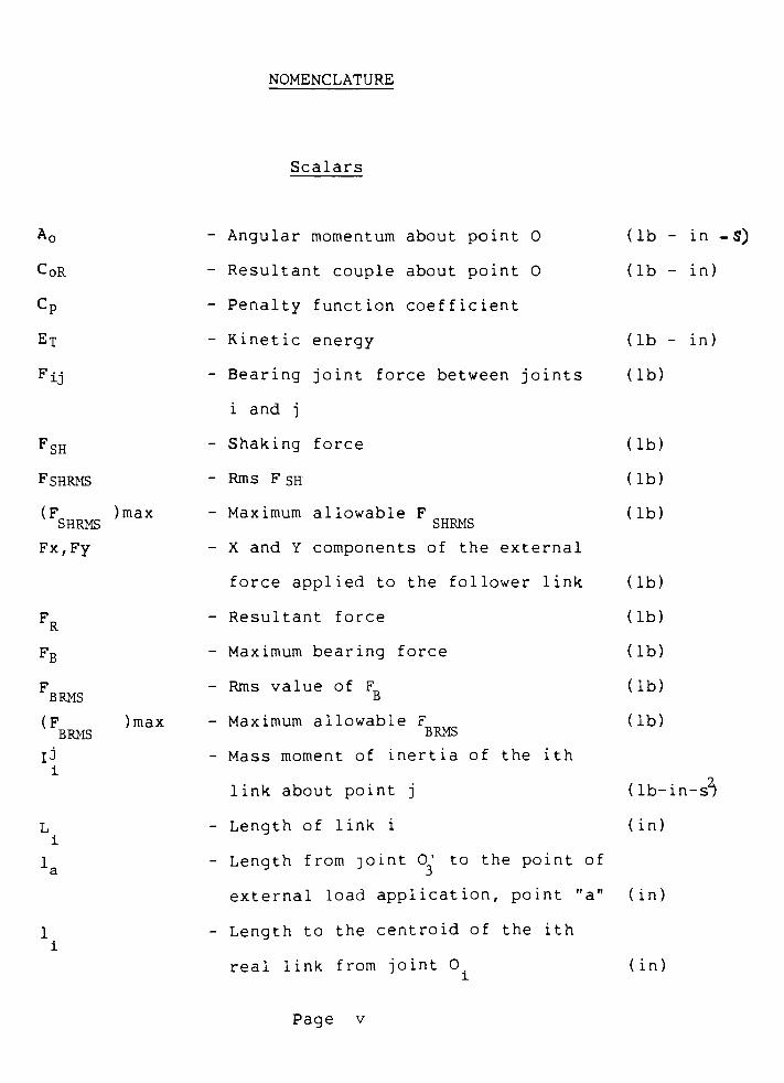
NOMENCLATURE
Scalars
C0R
Cp
Ex
Fij
FSH
FSHRMS
(F )maxSHRMS
Fx,Fy
R
BRMS
(FBRMS
i
)max
-
Angular momentum about point 0
-
Resultant couple about point 0
-
Penalty function coefficient
- Kinetic energy
-
Bearing joint force between joints
i and j
-
Shaking force
- Rms F sh
- Maximum allowable FSHRMS
- X and Y components of the external
force applied to the follower link
- Resultant force
- Maximum bearing force
- Rms value of F
- Maximum allowable FBRMS
- Mass moment of inertia of the ith
link about point j
- Length of link i
- Length from joint0'
to the point of
external load application, point"a"
- Length to the centroid of the ith
real link from joint 0.
(lb - in -S)
(lb - in)
(lb - in)
(lb)
(lb)
(lb)
(lb)
(lb)
(lb)
(lb)
(lb)
(lb)
(lb-in-sft
(in)
(in)
(in)
Page v
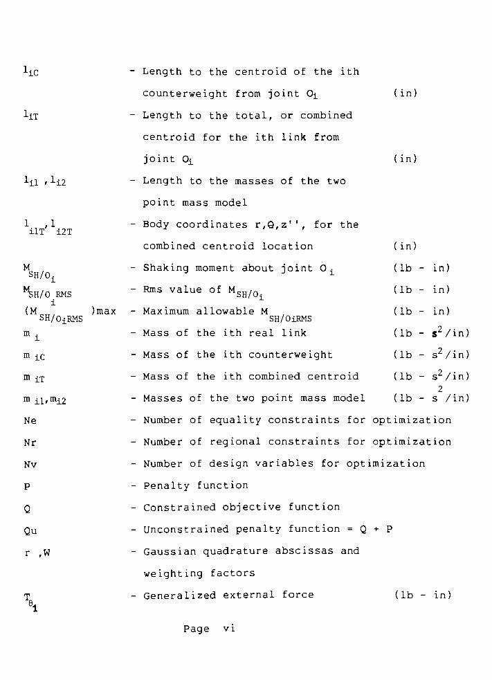
MSH/O
1
lie ~
Length to the centroid of the ith
counterweight from joint Oi (in)
liT -
Length to the total, or combined
centroid for the ith link from
joint Oi (in)
lil ' li2~
Length to the masses of the two
point mass model
1 ,1
-
Body coordinates r,Q,z'', for theilT i2T
combined centroid location (in)
-
Shaking moment about joint 0i
(lb - in)
H;h/o rms
" Rms value fMSH/0i
(lb - in)
i
(M ,)max - Maximum allowable M
,(lb - in)
SH/O-lRMS SH/OiRMS
m .
- Mass of the ith real link (lb -
s2/in)
m ic~ Mass of the ith counterweight (lb -
s /in)
m ix~ Mass of the ith combined centroid (lb -
s2/in)
2
m ll'mi2~ Masses of the two point mass model (lb -
s /in)
Ne- Number of equality constraints for optimization
Nr- Number of regional constraints for optimization
Nv- Number of design variables for optimization
p-
Penalty function
Q- Constrained objective function
Qu- Unconstrained penalty function = Q + P
r ,W
- Gaussian quadrature abscissas and
weighting factors
T- Generalized external force (lb - in)
91
Page vi
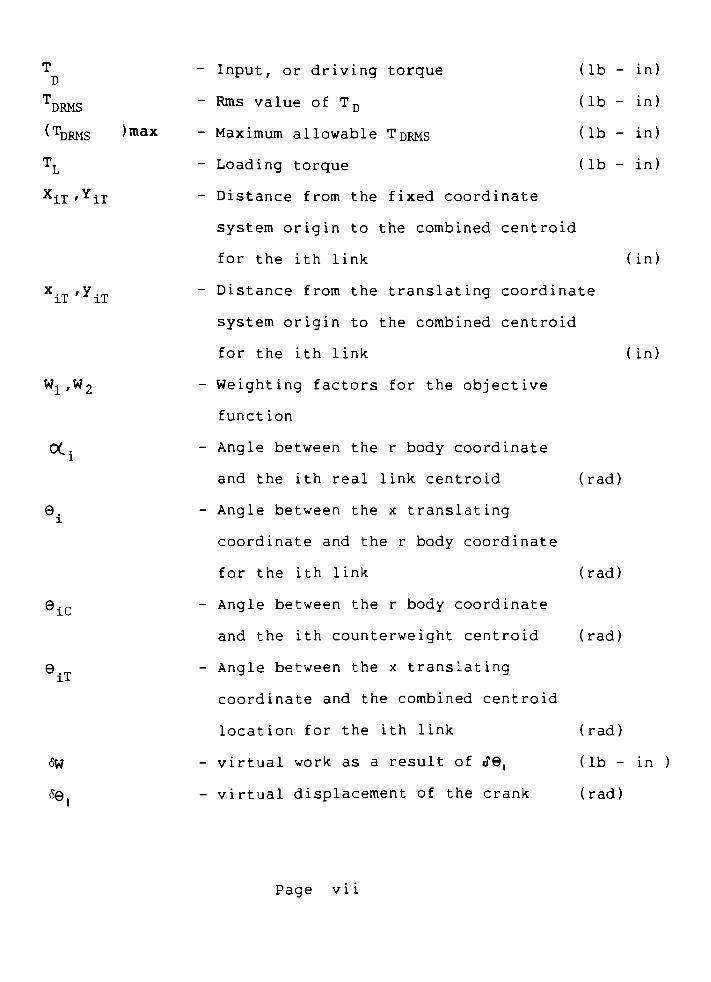
-
Input, or driving torque
DRMS
(TDRMS )max
TL
XiT ,YiT
x ,y
ITJiT
wlfw2
OL:
e
e
e
iC
IT
6W
60
-
Rms value of TD
(lb - in)
(lb - in)
Maximum allowable T^rms (lb ~
*n)
Loading torque (lb - in)
Distance from the fixed coordinate
system origin to the combined centroid
for the ith link (in)
Distance from the translating coordinate
system origin to the combined centroid
for the ith link (in)
Weighting factors for the objective
function
Angle between the r body coordinate
and the ith real link centroid (rad)
Angle between the x translating
coordinate and the r body coordinate
for the ith link (rad)
Angle between the r body coordinate
and the ith counterweight centroid (rad)
Angle between the x translating
coordinate and the combined centroid
location for the ith link (rad)
virtual work as a result of <?9, (lb - in )
virtual displacement of the crank (rad)
Page vii
*
*
*
*
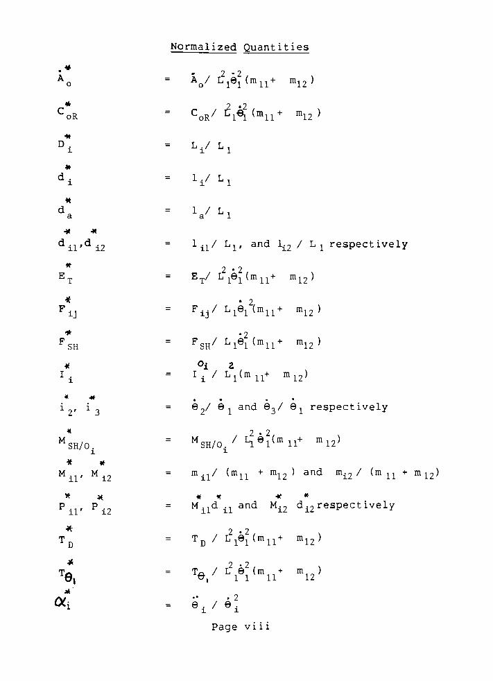
Normalized Quantities
"o_
n0fJJ1C'1^U11T'
"'12
2*2
Ao = A / L^e, (mn+ m19 )
CoR= C0r/ ^(mll +
m12 >
Dl=
Li/Ll
=
1/L1
da=
VL1
dil'di2=
'"il^ Ll' anci ^.2 ^ L1 respectively
*2*2
ET= ET/ L1e1(m11+ m12)
2,F.. = F../ L1e1(m11+ m12)
2
FSH= FSE/ Ll9l(mH+ m12>
* i 2
I. = Ii/L1(m11+m12)
* * ....
i,i_ = 2/ 81 and 3/ 6]_ respectively
MSH/0.= MSH/0./ Lll(mll+ m12>
* *
M..,
M.2
= m11/(m11+m12) and m2 / (m11
+ m 12)
P ,, P.= M.,d ., and M.9 d.9 respect ively
il i2 ii ii i^ -1-*-
2 -2
TD=
TD / L^dn^ m12)
.2 i2
Te,=
Te/Liei(mn+ mi2)
2
i' ~
ii = e, / e
Page viii
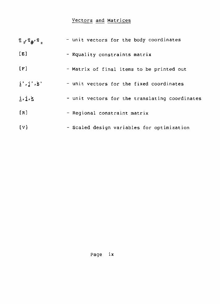
Vectors and Matrices
e , e ,e-
unit vectors for the body coordinates
[E] -
Equality constraints matrix
[F] -
Matrix of final items to be printed out
i',j',k'-
unit vectors for the fixed coordinates
i,2,k -
unit vectors for the translating coordinates
[R] - Regional constraint matrix
[V] - Scaled design variables for optimization
Page ix
Page 1
1.0 INTRODUCTION
Unbalanced linkages that operate at high speed, contain
massive links or experience large external loads may be
subjected to excessive vibration, noise and wear. Prediction
of the amount of imbalance is based upon the magnitude of the
shaking force, shaking moment, input torque and individual
bearing forces. Reduction of some or all of these kinetic
terms is desirable in balancing the linkage. There are many
different methods of balancing linkages, but most have only
been applied to the slider crank . Effective methods for
balancing linkages other than sliders, have only been
developed over the last fifteen years.
In 1969, Berkoff and Lowen [4] published a simple
technique for completely eliminating the shaking force. But
the method ignored the other kinetic effects, and often
increased the shaking moment and input torque. Berkoff, in
1973 [5], also developed a method that completely eliminated
both the shaking force and shaking moment in four bar linkages
with inline mass distributions. The technique, however,
required the addition of large geared inertia counterweights
which ended up doubling the mass of the linkage, and most of
the kinetic terms too. Reduction of the input torque has also
been accomplished by a number of methods. Most notably, the
use of a flywheel, which absorbs and transmits energy to
smooth out input torque fluctuations. But again, most of the
Page 2
methods gave little consideration to the remaining kinetic
quantities. Balancing of the combined effects is the next
logical step, but the equations involved are of sufficient
complexity that all practical considerations are limited to
computer applications. In 1975, Sadler [33] and others used
nonlinear programming to balance these combined effects.
Their results were in general better, and far more practical
than existing closed form techniques since regional
constraints could be used to limit many kinetic terms. None
the less, the formulation required separate optimization
trials for each quantity to be minimized, and a manual
development of trade-off curves to select the best overall
counterweight configuration. Additional schemes have been
presented since then, but most have not handled the problem as
efficiently and effectively as Lee and Cheng [21]. They chose
to minimize a single objective function expressed in terms of
the input torque and the ground bearing forces. Reduction of
the shaking force and shaking moment is also accomplished
since they are dependent upon the bearing forces. Lee and
Cheng also developed an efficient, closed form solution for
the kinetic analysis, and showed their method to be superior
to several existing techniques.
The objective of this thesis is to balance the combined
kinetic effects, using the theory presented by Lee and Cheng,
and to develop a general computer program which incorporates
their ideas. The analysis will be limited to balancing
planar, rigid body, four bar linkages through the addition of
Page 3
circular counterweights. The computer program is developed
from an existing optimization program written by R.C. Johnson
[18], and is modified to handle the general balancing theory.
Capabilities of the balancing program will be
demonstrated using three numerical examples. First, key
parameters of the program will be determined for an accurate,
but efficient analysis. The optimum number of sampling points
for numerical quadrature, and the degree to which emphasis may
be placed on individual terms, such as the input torque, will
be investigated. Results of the first example will then be
used in the second example. This example presents a practical
method of balancing an inline four bar linkage. The effect of
placing additional counterweights on the follower and coupler
links is also investigated. In the third example, a four bar
linkage with an offline coupler mass is balanced. The most
practical balancing scheme of the third example will then be
compared to the the unbalanced linkage, the method of complete
force balancing and the method of complete force and moment
balancing.

Page 4
2.0 LITERATURE SURVEY
The balancing of four bar linkages has been a problem for
both the designer and the researcher for many years. This may
be partially attributed to the complexity of the problem since
many different quantities must be taken into account (ie.
shaking force, shaking moment, input torque, bearing forces).
Various experimental and theoretical methods exist to balance
some of these parameters, but most have only been applied to
the slider crank family. Techniques for balancing linkages
other than sliders were not thoroughly summarized until 1968.
In that year Lowen and Berkoff [22] published a survey of
investigations concerning the balancing of four bar linkages
with special emphasis on mechanisms other than sliders. The
complete work categorized major techniques for balancing the
shaking force and shaking moment, listed 119 references, and
translated 11 important papers from Russian and German into
English. In 1977, Berkoff supplemented the initial survey by
publishing a summary of methods for determining and balancing
the input torque. In that paper, 71 references were cited and
major balancing techniques were described. With such
comprehensive literature surveys already published, the
efforts of this thesis will not try to duplicate either of the
above papers. Rather, the major techniques discussed in Lowen
andBerkoffs'
papers will be presented. In addition,
important theoretical methods for balancing planar, rigid body
linkages, published after the above mentioned summaries, will
Page 5
be discussed.
The method of balancing the Shaking force , or force
balancing, has been a popular method for many years. Lowen
and Berkoff [22] summarized many investigations where the
shaking force was completely or partially eliminated.
Complete force balancing attempts to make the center of
gravity of the linkage stationary, and can be categorized into
static balancing methods, method of principal vectors, cam
methods and duplicate mechanism methods. On the other hand,
partial balancing methods only reduce the shaking force, and
may be accomplished using harmonic balancing methods or by
adding springs to the linkage. Harmonic balancing methods use
a Fourier series and Gaussian least squares approach to
eliminate lower harmonics of the shaking force, while adding
springs to the linkage alters the path through which the
shaking force travels to ground. In 1969, Berkoff and Lowen
[4] published a new method for completely force balancing a
linkage termed the method of linear independent vectors. This
method was very easy to apply, and only required the addition
of two rotating counterweights fixed to the input and output
links. Lowen, Trepper, and Berkoff [24] in 1973 showed the
quantitative effects of complete force balancing a general
inline four bar linkage on other dynamic reactions such as the
input torque, shaking moment and bearing forces. The paper
also provided a complete tutorial on kinetic analysis
summarizing final equations and popular methods of analysis.
Oldham and Walker [31] in 1978, refined the method of linearly
Page 6
independent vectors by developing a method which automatically
chose the minimum number of counterweights for full force
balancing, without the derivation of kinematic equations.
Many others have extended Berkoffs initial work to practical
six bar linkages; Balasubramanian [3] 1978, Berkoff [6] 1979,
Dearstyne [10] 1983.
Although the method of force balancing significantly
reduces the net force on the frame, it may actually increase
the shaking moment. Lowen and Berkoff, in their initial
survey, described techniques for completely and partially
eliminating the shaking moment. Methods of complete shaking
moment balancing include cam actuated oscillating
counterweights, and the addition of a duplicate mechanism with
mirror symmetry. Also, harmonic methods were popular for
partially eliminating the shaking moment. Elimination of the
first, and sometimes the second harmonic of the shaking moment
was accomplished with two rotary masses which were
synchronized 180 degrees out of phase. In 1971, Lowen and
Berkoff [23] published a graphical method whereby the shaking
moment was minimized while maintaining a full force balance.
Complete force and moment balancing of inline four bars was
given by Berkoff [4] in 1973. This method, however, doubled
the total mass of the mechanism, and significantly increased
all other dynamic reactions. Wiederich Roth [43] in 1976
determined link inertial properties of a general force
balanced four bar linkage so that the amount of angular
momentum fluctuations, and hence the shaking moment, were
Page 7
minimized. Bagci [1] in 1980 extended complete force
balancing to offline four bars and some six bars using
balancing idler loops. These idler loops transferred the
effects of the coupler link motion to a ground bearing joint,
where Lancaster type balancers eliminated the shaking moment.
In contrast to balancing the shaking force and moment,
some balancing methods have concentrated on reducing the input
torque. Although it can never be eliminated totally, the
magnitude of torque fluctuations can be significantly reduced.
In 1977, Berkoff [7] summarized available methods of torque
balancing. As described by Berkoff, flywheels, spring
equivalents to flywheels, and cam subsystems are all capable
of smoothing out the torque curve. Each method stores and
discharges energy to reduce torque fluctuations. In
particular, cam subsystems can be designed to flatten out the
torque to perfection. Other methods summarized by Berkoff
include using torque regional constraints during kinematic
synthesis ( see [9] for example), and rearrangement of link
geometry by internal mass redistribution.
All the previous methods discussed have focused on the
elimination of one, or at most two balancing quantities.
However, as shown in various published example problems,
balancing of individual parameters may have an adverse effect
on other dynamic quantities, such as bearing forces. During
the mid 1970's researchers began attempting to balance the
combined dynamic effects of the shaking force, shaking moment,
input torque and bearings forces. Balancing of these combined
Page 8
effects is very difficult to achieve, but was facilitated by
the use of the digital computer. In 1975 Oldham [30], and
Smith [36], developed similar interactive computer programs
which provided full force balancing, and permitted the user to
manipulate link and counterweight properties to reduce other
dynamic effects. Conte, George, Mayne, and Sadler in 1975 [9]
used computer aided optimal design to generate mechanisms
through kinematic synthesis while minimizing individual
balancing quantities. Sadler [33] in 1975 also used nonlinear
programming to determine counterweight sizes and angular
locationSj while minimizing individual balancing quantities
through a series of optimizations. Once the effects of
minimizing individual parameters were known, trade-off curves
were used to determine which counterweight scheme resulted in
the best overall balance. Aside from digital computer
applications, Trepper and Lowen [38] in 1975 developed
equations for balancing the shaking force with flexible
constraints on ground bearing forces. These equations,
however, were of the 16th order and required extensive
computer work to be solved. Elliot and Tesar [11] in 1977
developed procedures for applying existing techniques in a
series of trials to determine which method provided the best
overall results. These trials were time consuming and
semiiterative in nature. Thus the problem of balancing the
combined effects seems best suited for the computer. However,
even with the aid of the computer, all of the previously
mentioned procedures required some manual iteration, and at
best were limited to minimizing only one quantity at a time.
Page 9
This problem was partially solved by Tricamo and Lowen [40] in
1983, who used automated optimal design to minimize the
maximum bearing force. The maximum bearing force was not
always limited to any specific bearing location, but varied
with counterweight arrangement. So, as the search process of
determining a counterweight configuration was carried out, the
actual location of the maximum bearing force was changing. In
addition, Tricamo andLowen'
s method placed regional and
equality constraints on other important balancing quantities,
such as the shaking force. The problem was further refined by
Lee and Cheng [21] who defined a general objective function in
terms of the ground bearing forces and the input torque. The
main idea behind reducing the ground bearing forces is to
balance the shaking force, shaking moment and two of the
bearing forces in one term. The input torque term was added
to incorporate sensitivity to that quantity. Parameters of
the counterweights were then determined using Heurisitic
computer optimization to minimize the objective function.
Example problems presented by Lee and Cheng showed their
method to be superior to force balancing, or force and moment
balancing. Comparisons to Tricamo andLowen'
s nonlinear
programming method showed Lee and Cheng's method to be
marginally better. The apparent success of Lee and Cheng has
led to the author's interest in developing a similar program,
and is presented in this thesis.
Page 10
3.0 OVERVIEW OF THE THEORY
The theory of balancing the combined effects of a planar
four bar linkage is divided into two parts:
1. The derivation of equations for the kinematic and kinetic
analysis. In particular, general equations for the input
torque, shaking force, shaking moment and bearing forces
must be found.
2. Development of the optimization problem, and application of
the existing automated optimization program to the specific
problem of balancing four bar linkages.
Equations describing the motion of the four bar mechanism
are obtained using vector analysis. This method is analogous
to the complex number method as presented by Shigley and
Uicker [34], Equations for the forces and couples are derived
by combining the Newtonian and Lagrangian approaches. This
method allows direct evaluation of all kinetic quantities
without the use of matrix solutions.
Once the equations for the kinetic analysis are known,
then the general optimization problem can be formulated. A
general objective function will be proposed, and a formal
statement of the optimization problem will be given. With the
problem defined, the techniques of automated optimal design
can be applied to determine the best location of the design
Page 11
variables (ie. radius and angular location of each
counterweight) so that the objective function is minimized.
The key assumptions of the theory are :
1. All links are treated as rigid bodies. Therefore, the
effects of stiffness, damping or natural frequencies have
been ignored.
2. The effects of gravity on the linkage have been ignored.
3. The linkage and counterweights are assumed to lie in the
same plane. Couples due to misalignment are not considered.
4. All links of the mechanism are assumed to have a finite
length. In otherwords, the analysis does not take sliders
into account.
5. Only circular counterweights of constant thickness and
density are used. Further, the counterweights can only be
attached tangentially to some of the bearing joints of the
linkage. Effects of the counterweight attachment brackets
have also been ignored.
6. All joints of the mechanism are lower pair, pin joints.
The term"linkage"
as defined by Shigley and Uicker [34],
mandates this assumption of lower pair contact.
7. The system is conservative. Thus the effects of friction
have been ignored.

Page 12
The validity of each of the above assumptions depends
upon the particular application and linkage to be balanced.
For example, the assumption of all the links being rigid may
not always be true for extremely high speed applications, or
where the stiffness of each link is relatively low in
comparison to the link mass. However, for many applications,
these assumptions provide a close approximation to the real
linkage, and facilitate a solution.
Page 13
4.0 DEVELOPMENT OF THE KINEMATIC AND KINETIC EQUATIONS
4.1 Two Point Mass Model
A general model of the four bar linkage to be balanced is
shown in Figure 1. It consists of three moving links and one
fixed link. Link 1 is the input or crank, link 2 is considered
the coupler, link 3 is the follower and link 4 is the frame. In
general, counterweights may be applied to any one of the moving
links at joints 0'-,, 0 ~, or O3. Circular counterweights of
constant thickness are shown as dashed lines in Figure 1. For a
general analysis, the link length, mass, thickness and
counterweight thickness, radius and angular location must all be
variable.
From an analysis point of view, a simpler yet dynamically
equivalent model of the real counterweighted linkage is the two
point mass model. First applied to mechanism balancing by
Wiederich and Roth [43], the model reduces the number of
variables for a general analysis. As shown in Figure 2, the
model consists of two point masses rigidly attached to the same
massless link. On each link, these masses are free to vary in
magnitude and distance, but are restricted to lie upon the given
body coordinate system axes. As shown in Figure 2, the first
mass must lie on the body"
r"
coordinate, and the second mass
must lie on the body" "
coordinate. The rules of vector
analysis still apply to the model, and the general configuration

Page 14
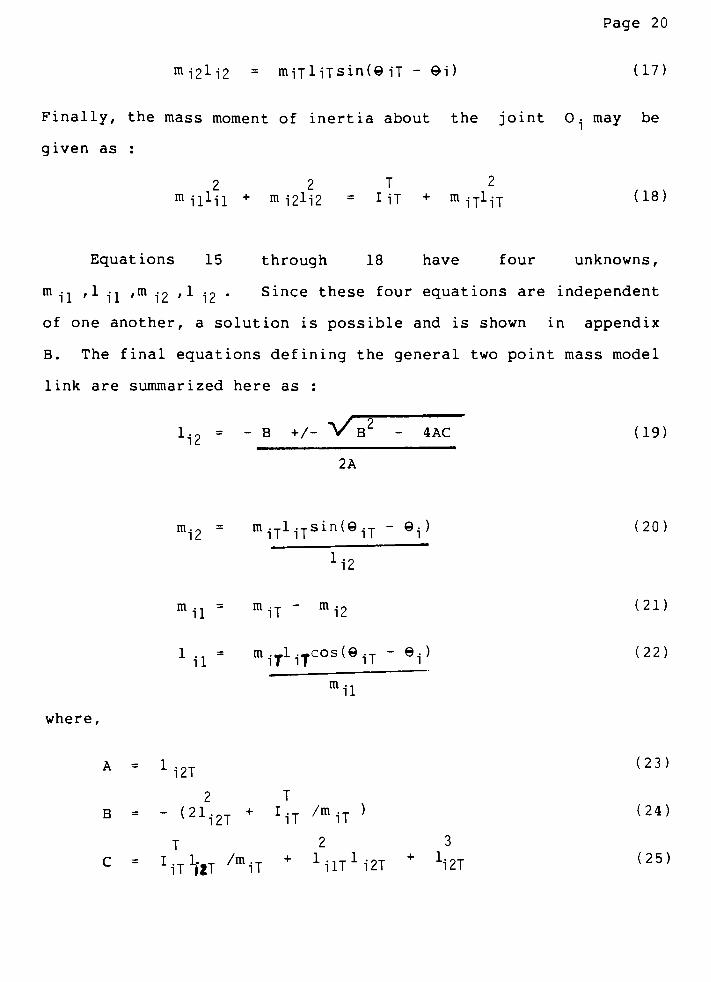
Figure 1 : General Four Bar Linkage with Circular Counterweights
LINK 1LINK 3
X X
Figure 2 : Two Point Mass Model
Page 15
of Figure 2 defines the positive locations of the masses.
As stated in [43], the inertial properties of any rigid body
can be represented by an equivalent system of point masses.
However, the model must obey all the basic laws of dynamics, and
be equivalent to the real linkage. The conditions for dynamic
equivalence between the real mechanism, and any equivalent model
require that :
1. The total mass of the ith link must be the same for
both models.
2. The center of mass of the ith link must remain in the
same location for both models.
3. The total mass moment of inertia of the ith link must
remain the same about the ith links centroidal location,
or about a bearing joint on that link.
In the above set of remarks, statements (1.) and (2.) ensure
Euler's first law of motion will be satisfied. The third
statement ensures that Euler's second law of motion will be met.
The additional statement in (3.) requiring the mass moment of
inertia to be the same about a bearing joint, not only includes
the frame joints,0'
and0'
,but also applies for joints 02 and
0 a This peculiarity is shown to be valid in appendix A.
The conversion from a real link with a counterweight to a
two point mass model link will be shown in a two step process.
First, with the real link and counterweight parameters known, an
equivalent combined center of gravity location will be
determined. This process is illustrated in Figure 3 for a

Page 16
general link rotating about a moving joint. This general case
describes link 2. However, if r'is a null vector, then the
analysis can be applied to links 1 and 3. With the properties of
the combined center of gravity known, the values of the two point
mass model may be found as shown in Figure 4. Each of these two
steps must obey the rules for dynamic conversions as stated
above.
Figure 3 : Combined C.G. Location of a General Link
with a Circular Counterweight
J counterweight
i combined e.g. location
\
In both Figures 3 and 4, there are several coordinate
systems ; the spatial XYZ coordinates, translating xyz
coordinates, and the body coordinates defined as r9z' '
. The
spatial coordinates are considered to be stationary with the
fixed set of stars, hence they do not have any angular velocity.
The xyz coordinates also don't have any angular velocity, but

Page 17
translate with the general point Oj . Finally, the r9z'
coordinates are fixed to the link so they translate and rotate
with the body. Unit vectors for each of the coordinate systems
are defined in Figures 3 and 4.
Figure 4 : Two Point Mass Model of a Combined C.G. Location
i combined eg location
*
%
Refering back to Figure 3, the total mass of the ith link is
just the sum of the real link and counterweight masses, or :
m
iTm. +
mic (1)
In addition, the x and y coordinates of the combined center of
gravity may be given as :
xiT=
iiT cos eiT
y.T=
liT sin 6iT
(2)
(3)
Page 18
Or, stated in terms of the real link and counterweight
parameters,
xiT=
micliccos(9i + Qic) +milicos(i +i ) (4)
mic+
rn,;
yiT=
micli sin(i+ eic) +
m1-lisin(ei+CX- ) (5)
mic+
mi
Squaring equations 2 and 3 separately, and adding the result
produces :
2 2 2
lU=
xiT+
^TT <6>
Substituting equations 4 and 5 into equation 6 for x^-i-and yiT
respectively, and solving for 1-T
:
liT=
[mZicl.2c+ + 2miclicmilicos(eic-0<i)] (7)
__
To obtain the value of-j , equation 3 is divided by equation 2,
and equations 4 and 5 are again substituted for x-T and y-T
respectively. The end result being :
Tan(iT) =
miclicsin(9i+ i(.) +
milisin(ei +OCi ) (8)
micliccos(1
+ .c) +
m.l1cos(ei +<Ki)
Last, the total mass moment of inertia of the real link and
counterweight must be determined about the combined centroidal
location, point T . Using the parallel axis theorem to transfer
the given mass moments of inertia,
t c 2 2
X1T=
{lic+
micC(xTc"
XiT> +
(*ic"
yiT> ] +

R 2 2
I.
+ m [ (x -
x ) + (y .
-
y._ ) ] }i i i ,T i iT
Page 19
(9)
where,
icxiT
=
liccos(9-j + e-jc)- lijcos(eiT) do)
y .
-
y =1 sin(<9 + ) - lsin(e._) (11)tc iT ic i ic iT iT
xj
-
xiT
= 1 i cos( i+ CX. i ) - lijcos(iT) (12)
y ] -y-jT=lisin(9i+0c^)- lijsin(iT) (13)
Substituting equations 10 through 13 into equation 9. and
simplifying the result yields :
T c 2 21iT
= * xic+
mic C xic + 1iT~ 21 ic liT cos(ei +
<ic-
iT ) ] +
R 2 2I +
mi [ 1-j + 1 iT-
21-j 1 iTcos(9 i + i-
iT) ] } (14)
The parameters given in equations 1, 7, 8, and 14 define the
total, or combined center of gravity which is dynamically
equivalent to a real link with a circular counterweight
tangentially attached. The remaining portion of this section
will be devoted to deriving the parameters of a general two point
mass model using the combined centroidal parameters. Refering
back to Figure 4, the total mass of the two point mass model is
given by :
mil+ mi2=iniT (15)
The centers of gravity for each of the^ two point masses, as shown
in Figure 4, may be given along the body coordinate axis (ie.
"r"
and "") as :
millil= m iTliTcos(iT
-
9-j) (16)
Page 20
m-j2l-j2= mijliTsin(9 iT
-
9i) (17)
Finally, the mass moment of inertia about the joint 0- may be
given as :
2 2 T 2
mil1il + mi2li2 I iT + m-jT1-jt
(18)
Equations 15 through 18 have four unknowns,
m ., ,1 -, ,m jo ,1
.. Since these four equations are independent
of one another, a solution is possible and is shown in appendix
B. The final equations defining the general two point mass model
link are summarized here as :
?/- V7~-li2
= - B +/- V B - 4AC (19)
2A
mi2=
miTliTsin(9iT-
Q.) (20)
~2"
mil=
miT"
mi2 (21)
1.1=
miTliTcoS(9iT- 9.) (22)
"
m~^
where,
A -
li2T(23)
2 T
B = -
(21i2T+
IiT /miT ) (24)
T 2 3
C =
^T^T /miT+
^-lT1!^+
hzi {25)
Page 21
The parameters of the two point mass model should obey the
equations summarized above for dynamic equivalence with the real
linkage. However, solution of these equations is not always
possible. There exists three special cases that are worthy of
consideration. First, if"
A"in equation 19 is zero, then 1
-2
becomes infinite. This case is easily solved by rederiving the
equations of the two point mass model with 1-j2J= * Another
2problem arises if B < 4AC. In that case the model for all
practical purposes is invalid, and will not provide an accurate
analysis. This problem is avoided in the OPTBAL program using a
2regional constraint which requires B > 4AC. Lastly, a
limiting situation arises when 1-j
=0. As discussed by Wiederich
and Roth [43], the initial conditions which dynamically define
the model, will not be obeyed in a practical sense. Fortunately,
it is very difficult to calculate a number of 0.0 exactly using a
computer, and the problem has never occurred in actual operation
the OPTBAL program. If such a situation would occur, the program
writes an error message to the user.
Now that the parameters of the two point mass model have
been defined, the next process in solving the overall problem is
to determine the kinematic equations for the four bar linkage.
This topic is covered in the next section using vector analysis.
Page 22
4. 2 Kinematic Analysis
The kinematic analysis of a four bar linkage will yield
equations for the angular position, velocity and acceleration
of links 2 and 3. For the analysis, the angular position,
velocity and acceleration of link 1 are assumed to be known.
The procedure will use vector analysis to derive loop
equations for the position analysis. Equations for the
velocity and acceleration will then be found by taking
successive time derivatives of the position equations.
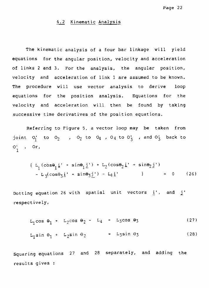
Referring to Figure 5, a vector loop may be taken from
joint0'
to 02 , 02 to O4 , O4 to0'
, and O3 back to
0'
. Or,1
{ L (cosi'
+ sin 2') +L2(cos2i'
+ sin2j')
-
L3(cose3i'
+sin3j_'
) -
L4 i'
} = 0 (26)
Dotting equation 26 with spatial unit vectors'
, andj_'
respectively,
Ljcos Q1+ L2cos 2
-
L4= L3cos 3 (27)
L^sin -L+ L2sin
-02= L3sin 3 (28)
Squaring equations 27 and 28 separately, and adding the
results gives :

Page 23
r r
2 2 2 2iL1+L2- L3+ L4+ 2 L1L2cos(i- 2)
- 2 L L.cos -9, 2 L2L 400s 92 } = 0 (29)
Figure 5 : Stick Figure of a Four Bar Linkage
Letting ,
2 2 2 2Li + L
2-
L3+ L4
- 2 L1L4cos &i (30)
Equation 29 now becomes,
A +cos92[2L1L2cos1
- 2L2L4] + sin2[2 L1L2sinjj] = 0
where 2
cos 2= 1 - Tan ( 9 2/ 2)
2
1 + Tan (9 7/ 2)
(31)
(32)
sin 2= 2 Tan (Q2/ 2)
-
1 + Tan (9-9/ 2)
(33)
Page 24
The analysis may be simplified even further by defining :
B = 2 L1L2cos i-2 L2L4 (34)
C = 2 L^sin 9i (35)
Substituting equations 34,35, and the 1/2 angle formulas into
equation 31 produces :
2A + B[l -
Tan(92/2)] + C[ 2Tan(92/2 ) ] = 0 (36)
1 + TanT2/2) 1 + Tan( /2)L
2
Simplifying,
Tan? 0/2) [ A -
B] + Tan(2/2)[ 2C ] + [ A + B] = 0
Equation 37 is of the form where Tan(92/2) may be solved for
using the quadratic formula. Or,
(37)
V? 2 2
._,_,, _, --
C - A + B (38)2'L
A - B
In the above equation A, B, and C are all known quantities so
99can be determined using equation 38. Once 92 is known, 3
can be easily found by dividing equation 28 into equation 27.
Or,
Page 25
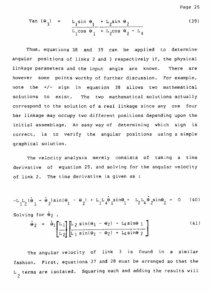
Tan (9 ) = L sin 9 + L sin (39)
L cos 9 + L cos
2-
L4
Thus, equations 38 and 39 can be applied to determine
angular positions of links 2 and 3 respectively if, the physical
linkage parameters and the input angle are known. There are
however some points worthy of further discussion. For example,
note the +/-sign in equation 38 allows two mathematical
solutions to exist. The two mathematical solutions actually
correspond to the solution of a real linkage since any one four
bar linkage may occupy two different positions depending upon the
initial assemblage. An easy way of determining which sign is
correct, is to verify the angular positions using a simple
graphical solution.
The velocity analysis merely consists of taking a time
derivative of equation 29, and solving for the angular velocity
of link 2. The time derivative is given as :
-L L (9 - 9 )sin(n- ) + L L sin + L L 9 sin = 0 (40
121 2 1 2 141 1 242 2
Solving for 2 ,
2= if*L
i"JJL 2 sin(i
- 2)- L4sin 1 1 (41))lfL
i"|[L 2 sin(i
- 2)- L4sin 1 1
|l2J [l 1 sin(i- 2) + L4sin 2 J
The angular velocity of link 3 is found in a similar
fashion. First, equations 27 and 28 must be arranged so that the
L terms are isolated. Squaring each and adding the results will
2

Page 26
then produce the following :
2 2 2 2i Ll + L3 L2 + L4
- 2 LlL4cos 9 1
+ 2 L^cos93
- 2 I^L^os (2-
3 ) } =0 (42)
Taking a time derivative of equation 42 will facilitate obtaining
9 . Thus,3
*9
LiL41sini-L3L493sin93+ LiL3(9l
-
3)sin(9 "63)= 0 (43)
Solving for 93 ,
e3=
1 rLi"|[L3sin( 91-
3) + L4sin9ll (44)
LL3jLLlsin( 9 e3) +
L4sine3J
The derivation of angular acceleration for links 2 and 3 is
accomplished by taking time derivatives of equations 41 and 44
respectively. The derivation will be made easier with the
following definitions. Let,
D( 9i,92) = fLllfL2 sin(9i-
2)-
L4sin ,1 (45)
[l J[l1sin(01
-
92) +
L4sin J
E( ei'93) =
[LllfL3 Sin(9l~
93) +
L4sineil <46>
lL3JLL! sin(1
-
3) +
L4sin3 J
Equations 41 and 44 may now be rewritten in terms of D and E.
2= D( 1, 2) 1 (47)
3= E( ^
3) 1 (48)
Angular accelerations can now be found by taking time derivatives
of the above two equations, or :
2=
D(9X, e2) i + D(!, 2) 1
e3=
E(elf 93)ex
+ e^, 3) ^
Page 27
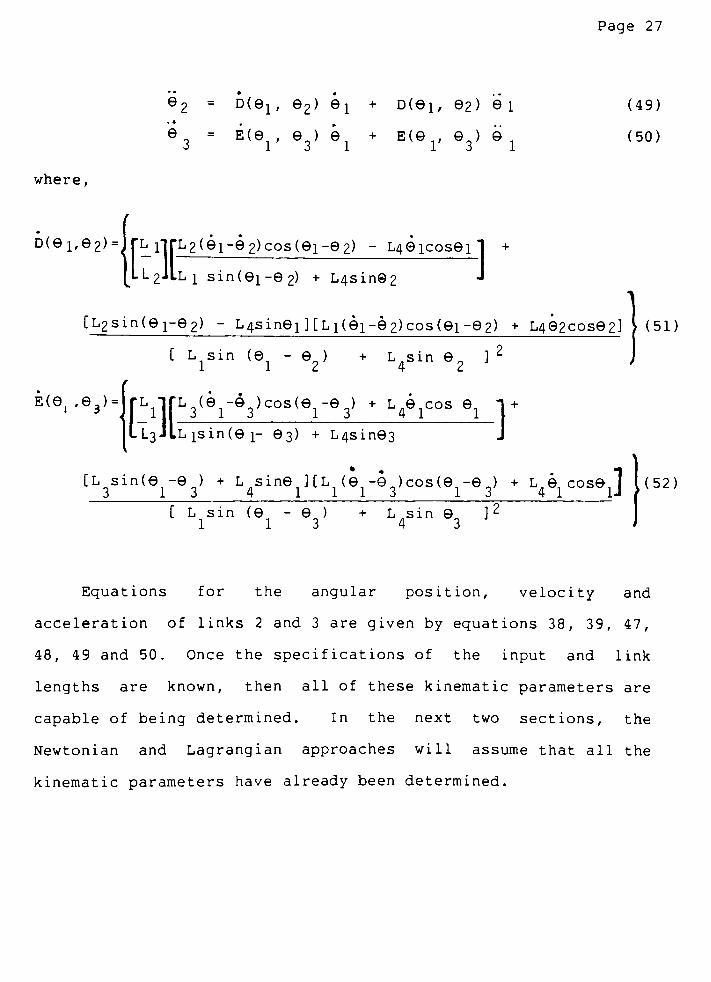
(49)
(50)
where,
D(i,2) = lrL i"J("L2(i-2)cos(i-2) - L4icosi"l +rLnrLgOi-
LL 2JLL 1 sin (l-2) + L4sin2
[L2sin(!-2) -
L4sini][Li(i-2)cos(i-2) + L42cos2J > (51)
E((,3)=
[ L^in(i
- e ) + L4sin2 ]
2
[Li][L3(4rd3)cos(6re3) + L4^icos61 1
+
L L3 JLl isin(1-
3) + L4sin3 J
[L sin( - ) + L sine ][L (0 -9 )cos(9 -e ) + L cos J [(52)
[ L sin ( - ) + L sin ] 2
1 13 4 3
Equations for the angular position, velocity and
acceleration of links 2 and 3 are given by equations 38, 39, 47,
48, 49 and 50. Once the specifications of the input and link
lengths are known, then all of these kinematic parameters are
capable of being determined. In the next two sections, the
Newtonian and Lagrangian approaches will assume that all the
kinematic parameters have already been determined.
Page 28
4.3 Newtonian Approach
The Newtonian approach uses Euler's first and second laws
of motion to derive equations for bearing forces and couples.
The laws will be applied to each of the three moving links,
which have two masses each. As shown in Figure 6, the general
configuration has external forces and torques applied to it.
Forces Fx and Fy are applied to point"a"
on the follower
link, while a loading torque, T^ , and a driving torque, To ,
are applied to joints0'
and0'
respectively. There are four
unknown bearing forces, each with spatial X and Y components.
Therefore, eight unknown components of the bearing forces need
to be determined. In addition the input torque is assumed to
be unknown. Once each of the links has been analyzed
separately, the four bar linkage will be analyzed as a whole
using the combined approach .
Euler's first law of motion as applied to a system of n
point masses may be written as :
-E!r=
2- mk^-k (53)
where,
F is the resultant force vector of externally applied
K
loads.
m is the mass of the kth point mass of the system.
k
r is the absolute acceleration of the kth point mass.
k

Page 29
Figure 6 : Free Body Diagram of a General Two Point
Mass Model
-FV w
0'
43 Y
^F43Y J~
41YJ"k SI__
A-
Fi'
' -F,
i' Xi'
41X1 43X1
*LD"
'-4
Page 30
Considering anyone of the 3 moving links as the system,
equation 53 can be rewritten as :
^Ri=
miklik (54>
where i = 1, 2, 3. Euler's second law of motion for a system
of n point masses may be written in general as :
ft
R=
2- o'k x m^ r_|< (55)
K--I
where,
C0r is the resultant couple vector, or moment about the
fixed joint 0.
,.is tne absolute position vector from point O'to the kth
particle of the system.
For a system of 2 particles, or point masses, rigidly
fixed together and rotating about a frame joint, Euler's
second law reduces to :
^'R =I 1-ik/o'X
m- r- (56)
K-11
where i = 1, 3. Equation 56 is adequate for the application
of Euler's second law to either of links 1 or 3, since they
rotate about a frame joint. However, link 2 does not rotate
about a fixed joint and must be analyzed using a different
equation. Appendix A shows the derivation of Euler's second
law of motion for this case with the end result being :

Page 31
I [ ^2k/o2x
m2k^2k/o2+^2k/o2x m2k '0^ (57)
where,
C is the resultant couple vector about the point 0-o2R
H y
2
Point 0 is not fixed, but may have a velocity and
acceleration vector.
r^ is the position vector of the kth point mass on link 2
with respect to the point 02
is the relative angular acceleration of the kth point
C.K/ Un
mass on link 2 with respect to point 02 .
r is the absolute acceleration vector of point 02 .
-o2
Applying Euler's first law- as stated in equation 54, to
link 1 :
Fr,,
=
I m, IrII
- Rl L, Ik -Ik(58)
where,
F_R1-
(F41x* F21x
i'
+
(F41y+ F21y>
L'
(59)
2
X! mik^lk=
mi^H+
m12^12 (60)
KM
The absolute acceleration vectors, r , and, r12can be found
by taking time derivatives of the absolute position vectors,
r 1 1 /n
'
,and r . Where,
-11/01~
12/01
r -=1 (cosi'
+ sin9.j'
) (61)
-n/o111 i - l
-
Page 3 2
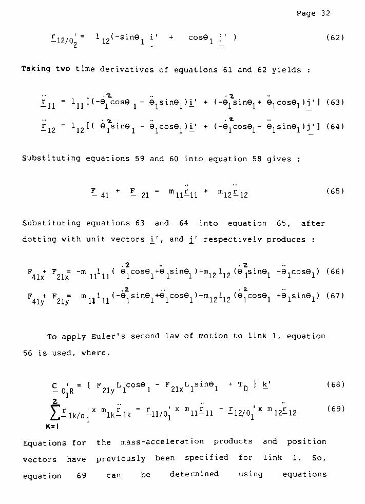
=
^(-sinGji*
+
cos1j'
) (62)
Taking two time derivatives of equations 61 and 62 yields :
.7. .i
-11
=
11 1cose
1
~iSinG.)^'
+ (-9,sin1+ ejcose^j'] (63)
-12
= 112^ Q^sin -cos.)^'
+
(-e.cose^ jsine^j'] (64)
Substituting equations 59 and 60 into equation 58 gives :
^41+
F- 21=
mll^ll+
m12^12 (65)
Substituting equations 63 and 64 into equation 65, after
dotting with unit vectors i_'
, andj_'
respectively produces :
.2 -2
F + F=
-m,1 ( .cos +9 ,sin9. )+m10 110 (91sin91 -9,cosQ,) (66)
41x 21x 11 11 1 11 1 1^ 1^ 1 11 1
.2.. 2
F + F = m.1,,
(-9,sin +9.COS9, )-m.-l10 (9.COS9. +9,sin9, ) (67)41y 21y 11 11 1 11 1 12 12 1 11 1
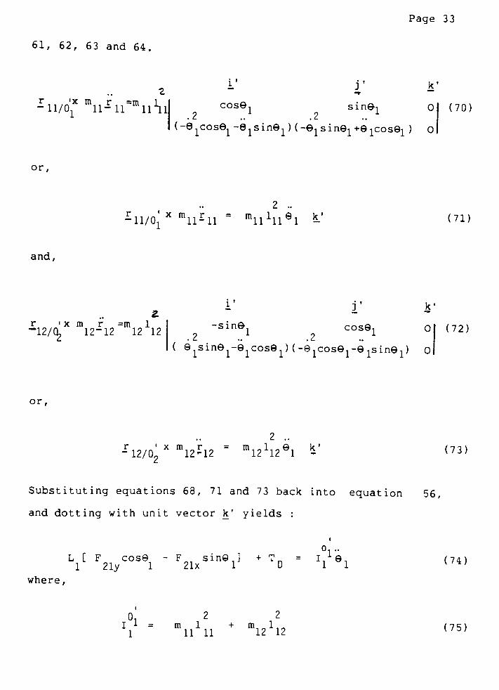
To apply Euler's second law of motion to link 1, equation
56 is used, where,
^0;R= { F21yLlCS6l'
F21xLlSin6l+
TD }*'
{68)
Eiik/0;xmik^k
=
in/0;x
mn^n+
^2/0;xmi2ii2 (69)
Equations for the mass-acceleration products and position
vectors have previously been specified for link 1. So,
equation 69 can be determined using equations
Page 33
61, 62, 63 and 64.
^ll/O^'u^ll-ll1!!
1/
cos9
k'
1 sine^ 0
.2 .2
(-1cos1 -^inej ) (-jsingj+e^os! ) 0
(70)
or,
2 ..
r...y
x m^r,,=
m^l^e,k'
-11/0, 11-11~
M,llxlll (71)
and,
r ' x m r =m 1
^12/0*^ 12-12 12 12-sin9
1
I
cos91
k'
0
.2 ..
x
.2
( 1sin1-1cos1)(-91cos1-1sin1) o
(72)
or,
-ri2/02Xmi2^12
=
ml21126'l*'
(73)
Substituting equations 68, 71 and 73 back into equation 56,
and dotting with unit vectork'
yields :
L [ F cos
1 21y 1F sin J + T21x 1 D
o .
ll 91
where,
(74
ii -
2 2
ro 1 + m, 1,11 11 12 12
(75)
Page 34
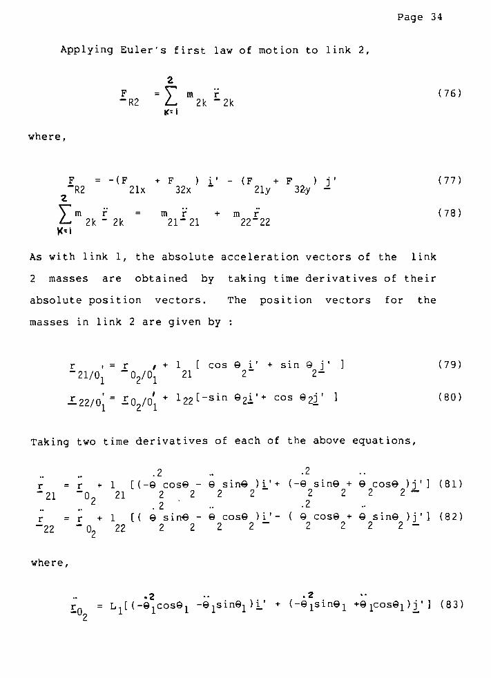
Applying Euler's first law of motion to link 2,
2
F = V m r (76)-R2 L. 2k "2k
K-1
where,
F =-(F +F )i'-(F +F
)j'(77)
"R2 21x 32x**
21y 32-y-
2
Zm r = m r + m f (78)2k
~
2k 21~21 22"22KM
As with link 1, the absolute acceleration vectors of the link
2 masses are obtained by taking time derivatives of their
absolute position vectors. The position vectors for the
masses in link 2 are given by :
r .= r /
+ 1 [ cosi'
+ sinj'
] (79)
~21/01 ~02/01 212"
2-
22/oj=
i^/o'*/l22[-sin 92i'+ cos
e22'
1 (80)
Taking two time derivatives of each of the above equations,
2 --2
r = r + 1 [(- cos -
sin )i'+ (- sin + 9 cos )j'] (81)
"21 -0, 21 2 2 22"
2222-
..
22
'
-2
r = r + 1 [( sin-
cos)i'- ( cos + sin )j'] (82)
-22 "02 22 2 2 2 2"
2 2 2 2-
where,
=
l,[(-1cos1+ (-isini +9
iCosi )j^'
] (83)

Page 35
Substituting equations 77 and 78 into equation 76,
(F., + F^)i'
+ (F + F)j'
=-m r
-
m r (84)21x 32x
-
21y 32y- 21-21
22~
22
Substituting equations 81, 82 and 83 into the above equation
after dotting with unit vectors , andj_'
respectively
produces:
.2
F + F = {(ni + m )L (9 cos9 + sin9 )21x 32x 21 22 1 1 11 1
+m2il21 (2COS2+ 2sin2)
+ m 1 (-9 sin + cos )} (85)22 22 2 2 2 2
.2
F + F = {(m + m )L (9 sin9- 9 cos9 )
21y 32y 21 22 1 1 11 1
+ rn 2 1 12 1 (92sin92-
92 cos92 )
'Z.
+ m 1 (9 cos9 + 9 sin9 )} (86)22 22 2 2 2 2
Euler's second law of motion, as stated in equation 57,
can be applied to link 2. Referring to the free body diagram,
Figure 6, the sum of couples on link 2 at joint 0- is given
by:
C = { F L sin9- F L cos9 }
k'
(87)-
02R 32x 2 2 32y 2 2"
The first term of equation 57 represents the time derivative
of the relative angular momentum of the two point masses in
link 2 about point O^, and is given by :
(88)
2
) r xmr
L* ~2k/0o 2k"2k/09
{r xmr +r xmr }
"21/02 21 21/02 22/02 22"22/02

The last term in equation 57 can be stated as :
Page 36
I*KM
2k/02x
m2k^02= ^21/02x
m21^02+ ^22/02x
m22^02(89)
where,
-21/0
= 12i^cose2i-'+sine2i'
^
22/0
= 122^~sine2^'+ cose22'
^
(90)
(91)
Taking two time derivatives of each of the above two equations
produces,
.2 .. .2
-
21/0=
x21* (_e2cose2" 2sine2)
~
+ (_e2sine2+ 2COse2)-l'' (92)
.2 .2
122 ^ ( 2sin02~e2cos02)^'
+ (-e2COSe2~e2sine2)i'^ (93)
The equation for the time derivative of the relative angular
momentum for link 2 about point 0- can be found by
substituting equations 90, 91, 92 and 93 into equation 88.
I>Km
r xm r =<
2K/^ 2K"2K/^
]
m 121 21
k'
0cos sin
2 .. .2 ..
(-9 cos -92sin2) (-2sin92+2cos2)0
+m22l 22
j/
cos2
k'
0-sin2
.2-2
(2sin2 -2cos2) (-2cos2-2sin2) 0
(94)

or,
where,
I -2k/02x
m2k-2k/022 "
9 9
Page 37
(95)
I2=
m21l21+
m22l22(96)
The last term of equation 57 can be determined if equations
83, 90, and 91 are substituted into equation 89. Thus,
I-KM
r.,. xm., r
=
m, 1 , L,rZK/Oj
2k"
0 21 21 1
i
cos, sin,
k'
02
w
2.2 .. -2
(-cos - sin ) (- sin91+9;.cos91)0
or,
+m22l22 Ll
y
cos92
k'
0-sin92
.2 ..-2
(^ cose -e sine ) (-e sine -e cose J o
(97)
Vr xmr =JL fmo 1 C. cos( - ) -sin(9 -9 )1LT 2k/0o 2k~0o
l 1 21 21 1 1 22
1 1 Z
K*i2k/02 2k~02
+ m
22 221
['
sin( - ) -9 cos(9 (98)
Now, equation 57 can be evaluated by back substitution of
equations 87, 95 and 98.
.2
L2CF32xsine2"F32ycose2J= ^m21121Lltelcos(el"e2)-lsin(l-2) ] +
.2
m 1 Li[sin( -.)+. cos(-) ] +
22*
1 121 1222 22
(99)

Page 38
Referring back to Figure 6, the application of Euler's
first and second laws to link 3 will be very similar to the
analysis already presented for link 1. Both rotate about a
frame joint, and have 2 bearing forces and a torque applied to
that joint. The only difference, is that link 3 has an
external force applied to it. This results in an additional
term. Thus, except for the external force, application of
Euler's laws of motion to link 3 will provide equations of the
same form as for link 1. Substituting the parameters of link
3 into equations 66, 67, 74jand taking into account the
external force applied to link 3 produces the following
equations.
.2 .. -2
F +F3 +F32 =-m3i I-31 (e3cose3+e 3Sin93) +m32132 (3 sin3-3COS3 ) (100)
.2 .. -2
F +F3 +F32=m3, 1 31(
-3sin
3+3cos3) -m32l
32 (3 cos3 +3 sin3) ( 101 )
1
la(-Fxsin+Fycos)+L1(F32ycose3-F32xsine3) + T,_=
1^3^(102)
where,
32 2
x3= m31X
31+
m32132 (103<
The end result of the Newtonian approach is nine
equations (ie. equations 66, 67, 74, 85, 86, 99, 100, 101,
102) which specify the relations between externally applied
forces, and the point mass accelerations. If the physical
Page 39
geometry and kinematics were known, nine variables would still
remain ; two components of each of the four bearing forces
and the input torque. At this point a numerical elimination
process, such as the Gauss-Seidel method, could be employed to
find a solution to the nine unknowns. However, the solution
would only be good for one geometry. The goal of this thesis
is to find the optimum design, which usually requires
analyzing many different geometries ( often on the order of 50
to 300). Using the Gauss-Seidel method, or most other common
numerical techniques, would not be very efficient for solving
the optimization problem.
Lee and Cheng simplified the solution of these nine
equations using a combined approach. This method, called the
"direct"
approach, uses the Lagrangian to first determine an
expression for the input torque. The resulting equation is
only a function of externally applied forces, and inertial
terms generated by the linkages motion. Thus, the Lagrangian
approach is independent of the Newtonian approach and provides
a quick, closed form solution for the input torque. Once the
input torque is known, then the bearing forces can be found
using the remaining nine equations of the Newtonian approach,
and a back substitution method.
To simplify the derivation of the input torque by the
Lagrangian approach, normalized parameters are used. Since
expressions from the Newtonian approach will later have to be
combined with the Lagrangian equation, they too will have to
be normalized. Definitions of these normalizing parameters
Page 40
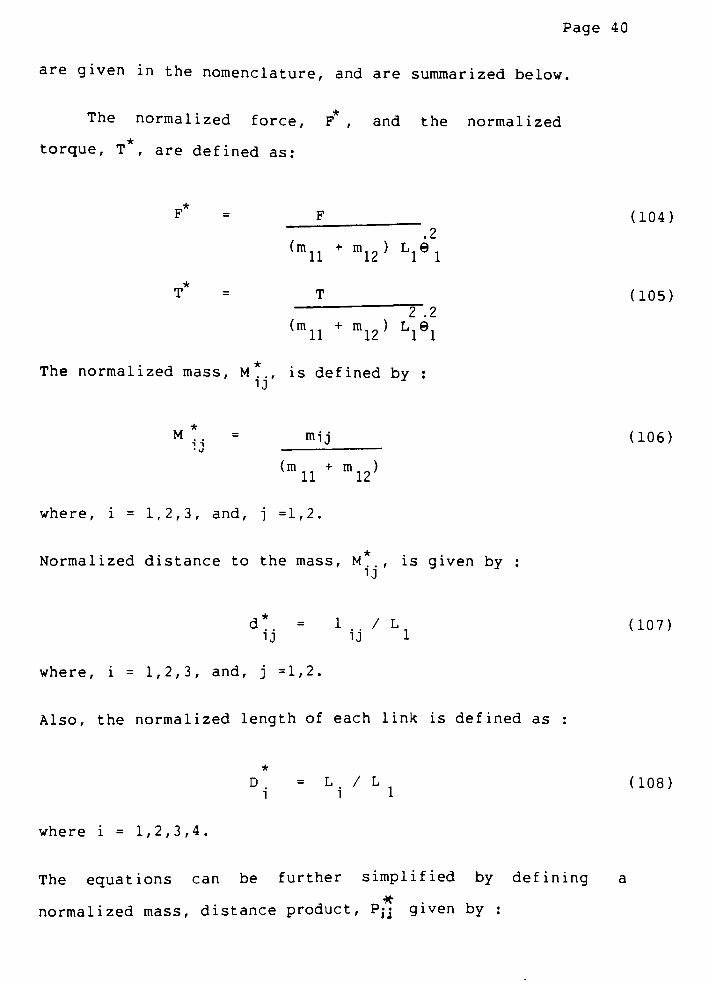
are given in the nomenclature, and are summarized below.
The normalized force,F*
, and the normalized
torque,T*
, are defined as:
F*
= F (104)
(mn+ m12) LlB1
T*
=
(105)
(mn+ m12) L1@1
The normalized mass, M.., is defined by :
M*
=
itiij (106), i
(mn+ m12)
where, i = 1,2,3, and, j =1,2.
*
Normalized distance to the mass, M, is given by :
d*. = 1../ L (107)
ij 1J 1
where, i = 1,2,3, and, j =1,2.
Also, the normalized length of each link is defined as :
*
D.
= L./ L (108)
l l 1
where i = 1,2,3,4.
The equations can be further simplified by defining a
normalized mass, distance product, Pjj given by :
Page 41
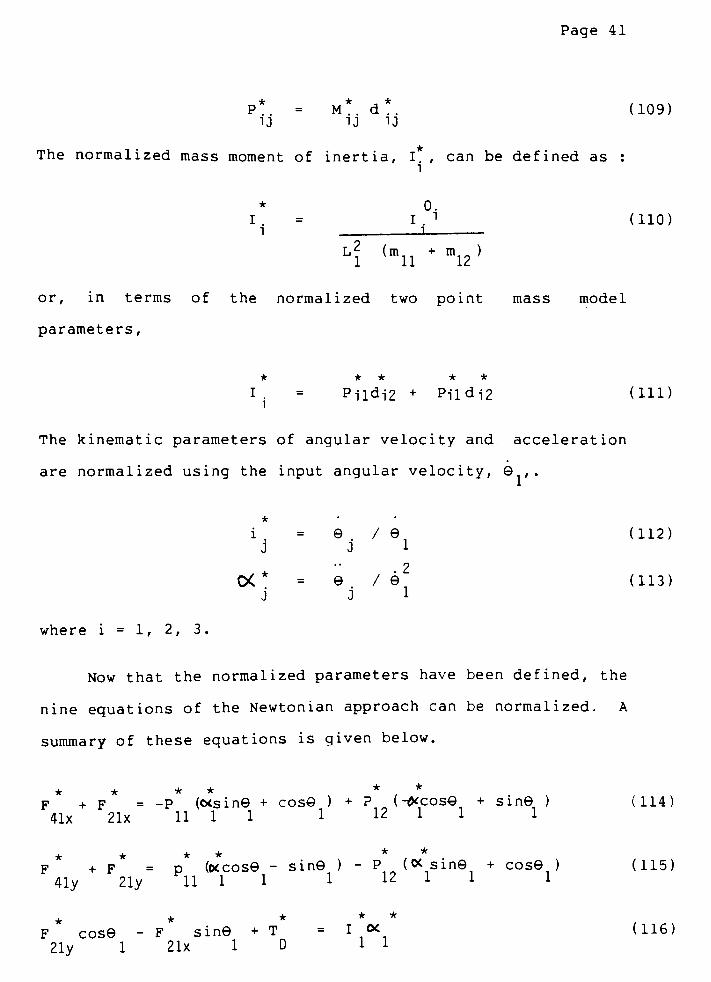
P*
= M*. d*. (109)
The normalized mass moment of inertia, I. ,can be defined as :
1
* 0.
I.
= 1.
1
1 1(110)
L? (mil+ mi2)
or, in terms of the normalized two point mass model
parameters,
* * * * *
I.
=
Pildi2 + Pildi2 (111)
The kinematic parameters of angular velocity and acceleration
are normalized using the input angular velocity, 9 ,.
(112)
(113)j J 1
where i = 1, 2, 3.
Now that the normalized parameters have been defined, the
nine equations of the Newtonian approach can be normalized. A
summary of these equations is given below.
* * * ** *
F + F = -P (<*sin + cos ) + P (-#cos + sin ) (114)
41x 21x 11 1 1 1 12 1 1 1
+ F = p (occos -
sin ) - P (<* sin + cos ) (115)?iv 11 1 1 1 12 1 1 1
*
i =
j j /ei
CX*
=
j9
j
. 2/
1
41y 21y 11 1 1
* ** *
F cos- F sin + T = I oc (116)
21y 1 21x 1 D 11

Page 42
FL+F32x=((M21+M22)(0<iSinei+
cos91)+P21(^sin92+ i22cos92)
+
P22(OC2S62" i*22sin92) } Ul7)
2F21y+F32y={(M21+M22)(_OClCOSei+
Sin6l )+*21 (^2COSV i2sin02)
+
P22(0<2Sine2+ i22cS92) } (118)
F3kD2*Sin92-F32yD2CS62= {
*K+ ^2l ^os^-^-siMe f^) ]
+
P22[*sin(91-
9) + cos^-^]} (119)
***** *2* *2
F 43x+F 32x=_Fx ~p 31<cx3sin93+ i3 cos93 ) + P32 (-0C.cos
+ i sin3) (120)
***** *2** *2
F +F =-F +P ((X. cos - i sin ) -
P (C< sin. + i_ cos ) (121)
43y 32y y 31 3 3 3 3 32 3 3 3 3
* * * ***** *
D3(F32ycos3- F32xsin3)= 130(3-
T[_ + da(Fxsin^-
Fycos^ ) (122)
Page 43
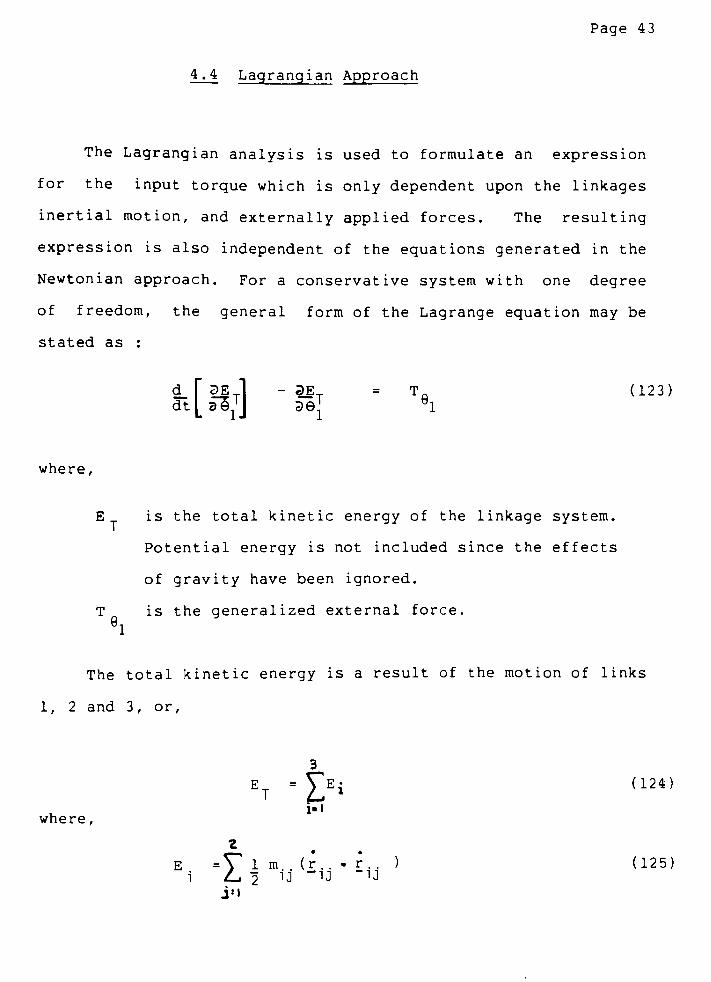
4 . 4 Lagrangian Approach
The Lagrangian analysis is used to formulate an expression
for the input torque which is only dependent upon the linkages
inertial motion, and externally applied forces. The resulting
expression is also independent of the equations generated in the
Newtonian approach. For a conservative system with one degree
of freedom, the general form of the Lagrange equation may be
stated as :
d r 3ETi -
3ET Ta (123)
3| Hl
where,
E is the total kinetic energy of the linkage system.
Potential energy is not included since the effects
of gravity have been ignored.
T is the generalized external force.
91
The total kinetic energy is a result of the motion of links
1, 2 and 3, or,
T "I
where,
3
I Ej (124)
c
E =V 1 m.. (r.. - r.. ) (125)
i L?M -U "U
y-\
Page 44
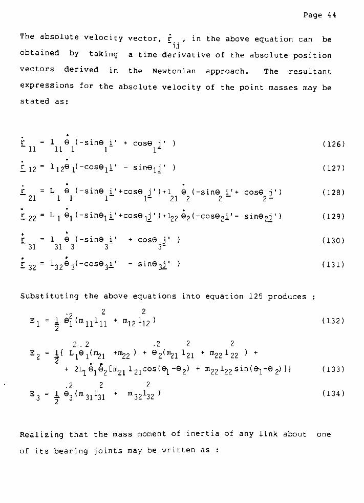
The absolute velocity vector, r,in the above equation can be
obtained by taking a time derivative of the absolute position
vectors derived in the Newtonian approach. The resultant
expressions for the absolute velocity of the point masses may be
stated as:
r = 1
"11 111
I 12" 1 12
1
r =
21
L 9
1 1
- 22=
L191
r =
"311
31 3
- 32=
132Q3
-sin i'
+ cos i'
)1-
-coseji'
-
sinejj'
)
-sin9 i'+cos j')+l (-sin i'+ cos j')1~
1-
21 22~
2-
-sin91 i/+cos9LJ'
)+l>2 92(-cos2i'-
sin92j'
)
-sin i'
+ cose j'
)3"
cos93_i_'
-
sine^j'
)
(126)
(127)
(128)
(129)
(130)
(131)
Substituting the above equations into equation 125 produces :
El=
\ ^^llhl+ m12112)
2.2 .22 2
E2= 1{ L^e^nu, +ITI22 ) +
2^ni2i 121
+
m22x
22^ +
+ 2L, i2 [m2, 1^cosfe^
-2) +
m22 122 sin(1- 2) ] }
.2 2 2
E3=
^S^Sl^l+
m32132 }
(132)
(133)
(134)
Realizing that the mass moment of inertia of any link about one
of its bearing joints may be written as :
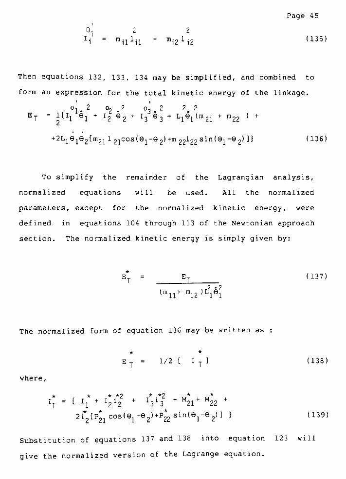
Page 45
o! 2 2
I-i=
milln+
^i2li2 (135)
Then equations 132, 133, 134 may be simplified, and combined to
form an expression for the total kinetic energy of the linkage.
1- 22 3 .
2 2. 2
et=
i{i1 e1+
i2 2+
i3 e3+
L1e1(m21+
m22 ) +
+
2L1192[m21 1 21cos(1-e2)+m22122
sin (6-^-62) ]} (136)
To simplify the remainder of the Lagrangian analysis,
normalized equations will be used. All the normalized
parameters, except for the normalized kinetic energy, were
defined in equations 104 through 113 of the Newtonian approach
section. The normalized kinetic energy is simply given by:
= E, (137)
2*2(HI-Q+
["12 )Liei
The normalized form of equation 136 may be written as
* *
Ey
= 1/2 [ IT
] (138)
where,
* * * *9 * *2* *
IT=
-
-1+
h'2+
X3l3+ M21+
M22+
2i*2[P21cos(e1-e2)+P22sin(e1-2)] } (139)
Substitution of equations 137 and 138 into equation 123 will
give the normalized version of the Lagrange equation.

Page 46
d_dt
2.2 ,
-^r litnin-i +m 12)L., e, i*l - JLfKm,, +m19 )L,eai[2
U u 1 l
TJ Zeh-1 12 1
2*)
J161 XT=
T91(140)
As evident from equation 139, IT is not a function of 9, .
Therefore, the normalized Lagrange equation may be rewritten as:
2 .23
*
(m +m )L g_ [9. L ] - 1 (m,. +m19 )L, e,-i [ IT ] =
Ta11 12 ldt 1 Ty
11 12 1
laQ)T 9X
(141)
Performing the necessary partial and full derivatives,
(mll+ml2)LlCVT+MjT] "
l(mll+m12)LieiC^T]=\
(142)
at z d9, i
where the partial derivative in equation 141 becomes a full
derivative since there is only one independent variable, 9, .
By the chain rule,
dt'
dei
dedt1
e di1
dej
(143)
Substituting the above results into equation 142, and
.2 2
normalizing (ie. dividing by &iLi(mn+
mi2 ^ ^> Produces the
following expression.
* * * *
CX I, + 1 dIT=
TaT
2deT
(144)
1
where,
T9l7 Ll9l(mll+ ml2) (145)
Using equation 139, the full derivative of IT with respect to e,
may given as follows:
*r* ** * **
dIT =Jl2t2i2di2] + I 3 [2i3 di3 ] +
d9l dex d9i
* *
+ 2 di2 [ P2icos(9i- 92) + P22sin(9i-
2)] +
a i
*
dej de x
However, using the chain rule,
d(e2 /ex ) d(e 2 /ei) . dei
dt dei dt
Rearranging the above expression,
d(e2/j) 1 d(2 /i)
dj i dt
where,
. 2dt i
Page 47
+ 2i2(l - i2) [-P2isin(i -92)+P22cs(ei-e2) ]} (146)
where,
di2 d(e2 / e i )
(147)
(148)
(149)
d(2 /ex) =
e2Q!-
2i (150)
Substituting equations 149 and 150, into equation 147 yields :
Page 48
* *
Ola =
c*2 hui dsi)
dex
similarly for link 3,
* * * *
di,3 - oc3-
i, *.d9,
3 3 I(152)
*
The full derivative of I with respect to the crank angle 9j can
now be obtained by substituting equations 151 and 152 into
equation 146. Or,
*
** * ** *** **
d!T = 2{ I2i2(CX2- i2c*i) +I3 i3 (OC
3- i3&<i) +
de1 * * * * *
+ (CX2- i20(i)[ P2iCOs(9!-92)+P22 sin(1-2)]* * * *
+ i (1 - i )[-p sin(9 -9 )+P cos(9 - )]} (153)2 2 21 1 Z 22 12
Using the above result, the Lagrange equation can now be
obtained.
* * * * *Z * *. * *
Tg,= {^[l
1+
I2i2+
I3i3+ M21+
M22+
1 * * *
+ 2i2[ P21cos(1-2) + P22sin(i-92
) ] ] +
* * * * * * * * * *
+I2i2(tt2- i2!) +
I3i3(CX3- i3^i) +
+ (C<2- i20(-i)[ P 21cos(el"e2)+P22
sin(1-2) ] +
+ i!(l -
i2 ) [~P2i sin(1- 2)+P22cos(1-2) ] } (154)
Simplifying ,
* *
TQ ^{(jClj+M21+M22+i2[P21cos(1-2)+P22sin(ei-e2)] ]
+
i2*+P2!cos(1-2)+P22sin(1-92) +
+
CX.*I*j^(1 -i*2)[-P 21sin(91-2)+P22COs(1-e2)]} (155)
Page 49
The above expression represents the generalized external force
in terms of the linkage motion. This generalized external force
may also be expressed in terms of actual external forces through
the method of virtual work.
TQ= J>W (156)
1 5 9!
where,
6W, is the external work done on the four bar mechanism
during a virtual displacement, 59i
69, is a small imaginary, or virtual rotation of the crank.
For the situation shown in Figure 7 of the combined approach
section,
6Wj= TL693+TD61
+ la(-Fxsiny&+ FyCOS^) ] 6 93 (157)
The generalized external force in equation 156 may be rewritten
as :
Trt = T + 53 [T, +1, (-FYsinfi+F cos ) ] (158)
9iD
-6;L a x r y r
The above expression is incapable of being evaluated since the
virtual displacements are imaginary. Thus, 53/6i must be
put into a more useful form. The ratio can be defined as the
virtual change in 3per virtual change in 9
,sand can be
determined usingkinematic equations. Equation 42 of the
Page 50
kinematic analysis relates the output and input angular
displacements by :
{L. -
L9 + L, + L- 2L,LCOS9
1 "2'
"3'
"4'"
"l^
+ 2L3L4cos93
- 2 L1L*3cos(1-9-,) }
1+
r3"uaior e3= o (159)
The above equation then can be differentiated to obtain a ratio
of the virtual angular displacements,
L1L4691sin91-L3L4693sin3+L1L3( 61"63 ) sin(1- 3) =0 (160)
Or, solving for 60 / 51 ,
63
_
61 LL3J
L3sin(1-3)
,L1sin(1-3)
+ L.sin*!
+
L4sin3J
(161)
The right hand side of the above expression is identical to the
ratio of the output to the input angular velocities, which is
given by equation 44 in the kinematic analysis. Therefore, the
ratio of the output to input virtual., angular displacements may
be given as :
6 = 1
6, 7
(162)
The final form of the generalized external force may then be
stated in terms of the angular velocity ratio given in the above
equat ion.
Page 51
'9i TD+ |i [T|_ +
lfl (-Fxsin^
+ Fycos) ] (163)
91
Normalizing,
Tfl= + C^ + ( -F*sinA+ F *cosfi) ] (164)\=
TD+
h^i +
da ( ~FxsinP>+ FycosP]
The end result of the Lagrangian analysis is an expression
for the input torque. This can be found by solving the above
equation for the input torque, Tn, or :
=
T9-," l3[ Tl
+ ("FxSinyS+ F^cosyB) ] (165)
*-
where TQ can be found using equation 155.
Wl
If the external loads and the kinematics of the linkage are
defined, then equation 165 provides an evaluation of the
normalized input torque for any particular geometry. Equations
for the bearing forces could then be determined using the nine
equations of the Newtonian approach and a back substitution
procedure. The combined approach, presented in the next
section, shows how the principles of angular momentum can be
applied to facilitate this process.
Page 52
4.5 Combined Approach
The nine equations derived in the Newtonian approach, and
the input torque expression obtained using the Lagrangian
approach do not provide a direct evaluation of the bearing
forces. In fact, these bearing forces are often solved for
using a numerical procedure, such as the Gauss-Seidel method.
In contrast, the"direct"
method proposed by Lee and Cheng [21]
provides a closed form solution of all the bearing forces using
a combined formulation of both the Newtonian and Lagrangian
methods.
The fundamental idea of the combined approach is to analyze
the four bar linkage as a whole using Euler's second law of
motion. In such a way, the Y components of each ground bearing
force are determined. Lagrange's method is used to provide an
expression for the input torque, Tn . Expressions for the
remaining bearing forces are then solved for using expressions
from the Newtonian analysis coupled with a back substitution
procedure.
To analyze the linkage as a whole requires a new free body
diagram. Figure 7 shows a two point mass model of the linkage
separated from its surroundings. Applying Euler's second law of
motion to the system of three moving links about the frame joint

Page 53
Figure 7 : Free Body Diagram of a Two Point Mass Model
Separated from its Frame
where,
0'R= {F43yL4 +TL +TD
-Fx1asinyB+
Fy ( lacoS/ +L4 ) }k'
(167
13
= 2_ li/0o!
The above equations can be evaluated if the angular momentum of
(168)
each link about joint0'
can be determined. This angular
Page 54
momentum can be found using the following relations
Ai-r ixm r +r ixmr
i/0. "il/0- il -il i2/0-12
i2(169)
where, i - 1, 2, 3. The angular momentum for link 1 can be
found by letting i = 1 in the above expression, thus :
A i =r ixmr +r x m f
""1/0, "11/0, 11-11 -12/0. 1212(170)
or,
A ,=
"1/0,
m ii 111Hi
m12 112
i_'
yk'
cosi sini 0
!Sini icos i 0
i'
y&'
-sini cosi 0
-lCOs9i -9isini 0
(171)
Simplifying,
1/0,
2 2
{(mnln + m12l12) i}ii'
(172)
Taking a time derivative,
1A ,
= { Ix 9i}k'
_i/o1
(173)
For the coupler, link 2, equation 169 can be written as,
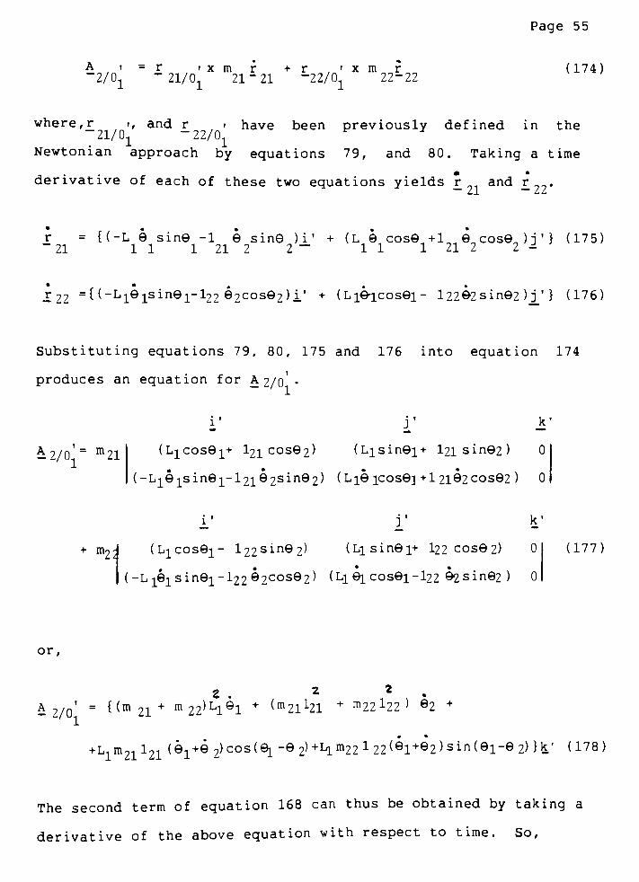
Page 55
A i = r ixmr + r 'xm?
-2/01-
21/01 21-21 ~22/0122~22
(174)
where, r i, and r i have been previously defined in the
_21/01~
22/01Newtonian approach by equations 79, and 80. Taking a time
derivative of each of these two equations yields r and r .
r = {(-L sin -1 sin)i'
+ (L 9 cos +1 9 cos9)j'} (175)~
21 11 1 21 2 2~
11 1 21 2 2 ^
r22 ={(-Liisini-l22
2cos2)i'+ (Liicos9i-
l222sin92 ) j'
} (176)
Substituting equations 79, 80, 175 and 176 into equation 174
produces an equation for A
b. 2/0=
m21
i' j' k'
(LiCOsei+ I21 cose 2) (Lisinei+ l2isine2) 0
(-Lieisinei-l2ie2sin2) ( LL9 icos9i +1 2ie2cos62 ) 0
Jk'
+m2^
(Licosei- l22sine2) (Lisin9i+ I22 cos9 2) 0
** *
(-Li9isin9i-l222cose2) < Ll 1 cosei~l22 e2 sine2 ) 0
(177)
or,
A = ^(m21+m22)Ll9l
+ (m21X21 +m22 L22 > e2 +
+L1m21l21(e!+92)cos(9i-92)+Lim22l22(l+e2)siri(9i-9
2)}k'
(178)
The second term of equation 168 can thus be obtained by taking a
derivative of the above equation with respect to time. So,
Page 56
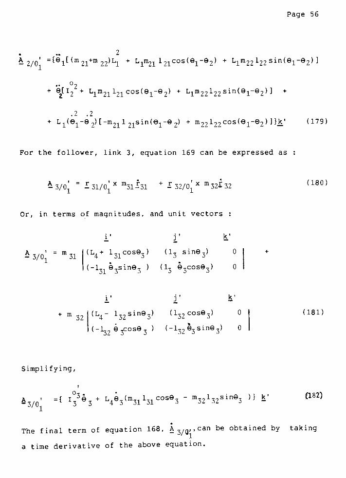
4ft^
=^l^ (m2i+m22^L1
+
Lim2i 121cos^el_e2^+ Llm22122 sin(9i-92)]
.. 2+
Jl2+
Lim2i 121 ^03(6-1^-92)+ Lim22122sin(el~e2^ +
.2 .2
+ L1(1-2) [-m21 1 21sin(1-2) +m22 122 cos(1-2 ) ] }k/ (179)
For the follower, link 3, equation 169 can be expressed as :
-3/0J
"
m3li31+ m
32-^ 32(180)
Or, in terms of magnitudes, and unit vectors
k'
m-
3/0, 31(L4+ l-.cos,) (13 sin93) 0
(-i31 e3sine3 ) Q3 e3cose3) 0
+ m32
i*
yk'
(l4- i32sine3) d32cose3) 0
(_132 3COse3* ("1323sin63)
(181)
Simplifying,
h/0 =[r333+ WV^l^l008^ m32132sine3 )} & (182)
The final term of equation 168, A3,g, ,can be obtained by taking
a time derivative of the above equation.
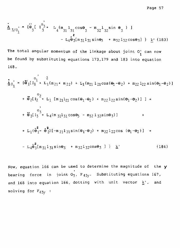
Page 57
t
A i = te [ lj>+ L (m 1 cose -ml sin e ) ]
3/01 3 3 4 31 31 3 32 32 3
*
-
L4e3[m3il3isin3 + 11132I32COS93] } k' (183)
The total angular momentum of the linkage about joint0'
can now
be found by substituting equations 173,179 and 183 into equation
168.
t
12
h.0^= ^"l^l + Ll(m21+ m22> + Ll(m21 l21cs(l-2) +
m22 122 sin(9i-92) ]
2+ 92[l2 +
Li [m2il2i cos(9i-92 ) +m22 122 sin(i-2 )] ] +
1
3+ 3[I3'+ L4(m
3il31cos3-
m32l32sin93)] +
.2 .2
+ Li(9i~ 9 2) [-m 2il2isin(9i-92) + m22l22cos (el_e2)] +
2-
L4e3[m31l3isine3+m32l32COS3 ] }
k'
(184)
Now, equation 166 can be used to determine the magnitude of they*
bearing force in joint O3 ,F43y. Substituting equations 167,
and 168 into equation 166, dotting with unit vectork'
, and
solving for F43 :
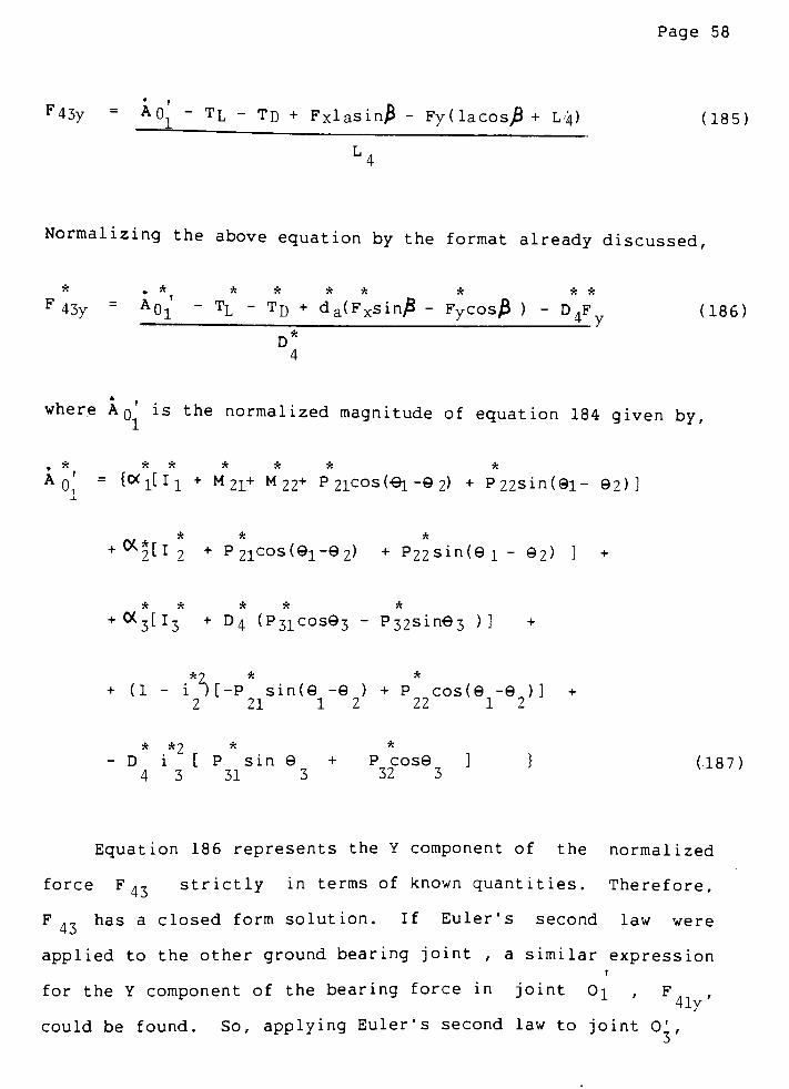
Page 58
F43y=
Aq-
Tl-
TD + Fxlasin,B -
Fy( lacos.fi + L4) (185)
L4
Normalizing the above equation by the format already discussed,
*.
* * * * * * * *
F43y=
A0i~
TL~
TD + da(Fxsin,6 - FycoS/B ) - D.F (186)
D*
JLv
where Aq is the normalized magnitude of equation 184 given by,
,* ***** *
A0.'
= t]_[!]_
+ M2i+ M22+ P 2lcos(!-2) + P22sin(i- 2)]
+ ^2[I2 + P2iCOs(i-2) + P22Sin(e!-
2) ] +
* * * * *
+ OC3[i3 + d4 (P3icos3-
P32sin3 )] +
*2 A *
+ (1 - i )[-P sin( -e ) + P cos(e -6 )] +
2 21 12 22 12
* *2 * A
- D i [ P sin e + P cose ] } (187)4 3 31 3 32 3
Equation 186 represents the Y component of the normalized
force F43 strictly in terms of known quantities. Therefore,
F., has a closed form solution. If Euler's second law were
applied to the other ground bearing joint, a similar expression
1
for the Y component of the bearing force in joint Oi , F41y'
could be found. So, applying Euler's second law to joint0'
,

Page 59
-iR*-i<188>
where,
~n'D
= {"F,1 La
+
Tn+
TT+ 1 (_F
sin+ F
cos >*Jl'
(189)0_R 41y 4D
Lax'y'
=
2^-i/0J (190)-3 ^-i,3
Substituting equation 189 into 188, dotting with unit vector k',
and solving for F41
F41y= {
"A03+
TD+
TL + la ("Fxsin^ +
Fycos ) } (191)
r4
where An'
can be obtained by a very similar analysis as that
3
already presented forAn'
. Normalizing equation 191,ul
F*ly= { -
Aq3h-
Tp+
TL+ da (-Fx sinfi*
Fy cosff )} (192)
B7
where,
a* = {Of [i- + m21+ m22+ P21cos(e1-e2) + p22sin(ei-e2) +
3
* * * * *
+D4[(-M2,-M22-P11 ) cose1
+Pl2 sinx ] ] +
Page 60
* * * *
+ OC [ i2
+ P21cos(i
-
2 ) + P 22sin( i-
2 ^ +
* A A A A
-
D4(P2iCOS2-
P22sin92)] + <-3l3 +
a?L
A A
+ (1 - i 2) [-P2isin(91
- 92) + P22cos(9i-
2 ) ] +
* A A A A
+ D [(M + M + P ) sin + P cos 9 ] +
4 21 22 11 1 12 1
A A2 A A
+D4 i
2t P?iSin 92 + P
22cos e
2 ^ * (193)
In summary, equations 165, 186 and 192 provide closed form
solutions for the normalized input torque, Tj) , and normalized Y
A A
components of each of the ground bearing joints, F43y and F4iy,
respectively- With these quantities known, the remaining
unknown bearing forces can be easily solved for using some of
the nine equations of the Newtonian approach, and a back
substitution procedure. The basic procedure is described below.
A
Knowing F*3 ,and the externally applied force on the
follower, equation 121 can be rearranged to yield an expression
A
for F_*,
.
32y
a * * *,
*. *2 . .
F32y= {
-Fy~
F43y+
P31 {fosQ3"
13sin93)
a * *2- P,- (Cx'7sin9, + i, cos 9,) } (194)
'32("f:
A
Once F is known using the above equation, then F32x can be
determined usingequation 122.
Page 61
F32x= {~I3oc3+
TL"
Fxdasin + Fydacos +
F32yDjcos^ } (195)
A
D3sin93
Rearrangement of equation 120 provides an expression for the X
component of the bearing force in joint O3 :
A A A A A A2
F43x=
*-Fx"
F32x"
P31<*3sine3 + ^^sQt,) +
A A A2+ P 32(-0<3COs9
3+ i3 sin93) } (196)
Also, since F4! is known, F2iy
can be obtained using equation
115.
A * * * A A
F2iy ={-F4iy +Pn(0<1cos1-sin91 )-P12 ((Xisin9i +cos9i)} (197)
A
The unknown component of the ground bearing force, F2ix ,can be
A
expressed in terms of F32x using equation 117. Or,
A * A * *
F21= * ~F32x
+ (M 21+ M 22* ^f in9l+ cos9i) +
A * *? A A A2+ p 21(0<2Sin2+ i2cos2) +
P22 (<*2cos9 -
i2sin92)} (198)
Finally, the normalized force F41x
can be determined by equation
114,
F = {-f71
-P11(0t,sin9,+cos91)+P12 (-0cicos91+sin9i)} (199)

Page 62
Since all the bearing joint forces are known, expressions
for the shaking force and shaking moments can be determined from
their basic definitions. The shaking force is defined as the
net force felt by the frame, while the shaking moment is equal
to the time derivative of the angular momentum vector.
^SH= {
-(F41x+
F43x+Fx>i'
"
(F41y+
FlzY+VI'
} (200)
^sh/0;= -
(A0;>
W-'
(201)
^sh/0;= -
(A0;> v (202)
Thus, all of the unknowns of the kinetic analysis can be solved
by sequentially applying the equations derived above.
The analyses of sections 4.1 through 4.6 have provided a
method of determining the input torque, shaking force, shaking
moments and the bearing forces. The overall objective of
balancing is to reduce or eliminate some or all of these
quantities. The next section will propose an objective function
which provides a qualitative evaluation of these quantities in
one equation. The goal of the optimization package will then be
to minimize that objective function, and thereby partially
balance all these important kinetic quantities.
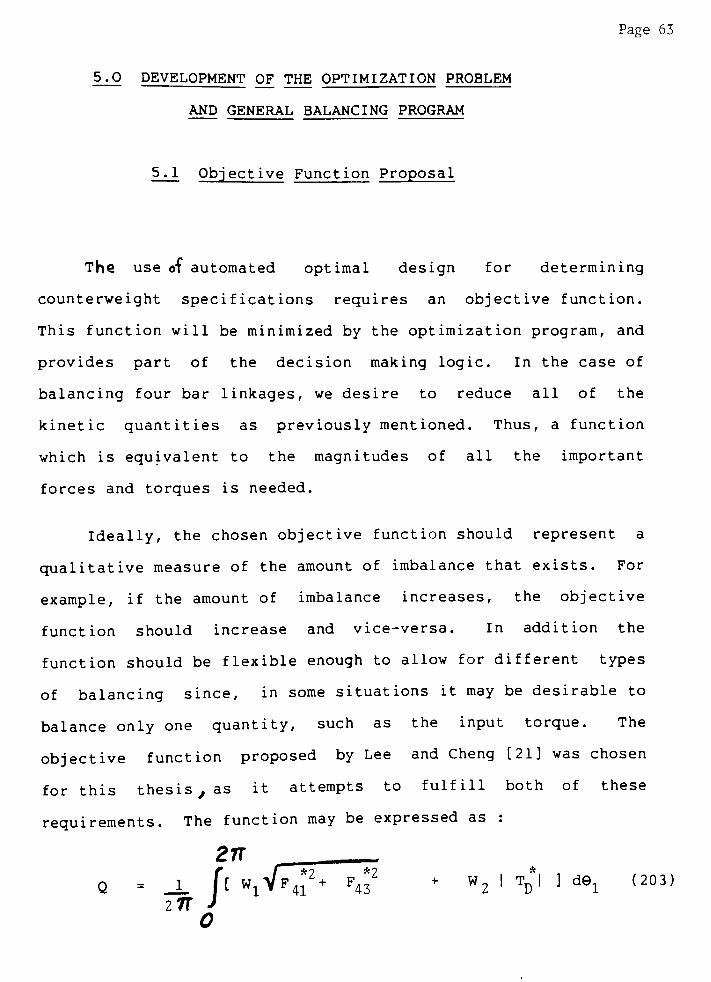
Page 63
5.0 DEVELOPMENT OF THE OPTIMIZATION PROBLEM
AND GENERAL BALANCING PROGRAM
5.1 Objective Function Proposal
The use of automated optimal design for determining
counterweight specifications requires an objective function.
This function will be minimized by the optimization program, and
provides part of the decision making logic. In the case of
balancing four bar linkages, we desire to reduce all of the
kinetic quantities as previously mentioned. Thus, a function
which is equivalent to the magnitudes of all the important
forces and torques is needed.
Ideally, the chosen objective function should represent a
qualitative measure of the amount of imbalance that exists. For
example, if the amount of imbalance increases, the objective
function should increase and vice-versa. In addition the
function should be flexible enough to allow for different types
of balancing since, in some situations it may be desirable to
balance only one quantity, such as the input torque. The
objective function proposed by Lee and Cheng [21] was chosen
for this thesis,as it attempts to fulfill both of these
requirements. The function may be expressed as :
21J
Q =
_i_
f[W1VF4*2
+
27T J
0
F4J2
+
W2 I TD*| ] d9x (203)
Page 64
As can be clearly seen, the function is a linear combination of
an equivalent ground bearings force and the input torque. Wi
and W2 are weighting factors which in theory, can be varied to
allow for emphasis on different parameters. The integration of
the function over the range from 0 to 2fT represents an average
of the objective function based on one cycle, or revolution of
the crank.
At first glance, the objective function would appear only
to be dependent upon the input torque and ground bearing forces.
But a closer inspection of the equations that define the shaking
force and shaking moment, would show that they are dependent
upon both terms in the objective function. Minimizing the
proposed objective function will, in effect, most likely
decrease all the important kinetic balancing terms. While the
proposed function does not give an exact representation of all
the kinetic parameters, it does provide a numerical value which
approximates the amount of imbalance in the linkage. The
validity of this statement can be seen in the successful results
of the example problems.
With a mathematical definition of the objective function to
qualitatively measure the amount of imbalance in the mechanism,
the remainder of the theory will formulate, and provide a method
to solve the optimization problem.
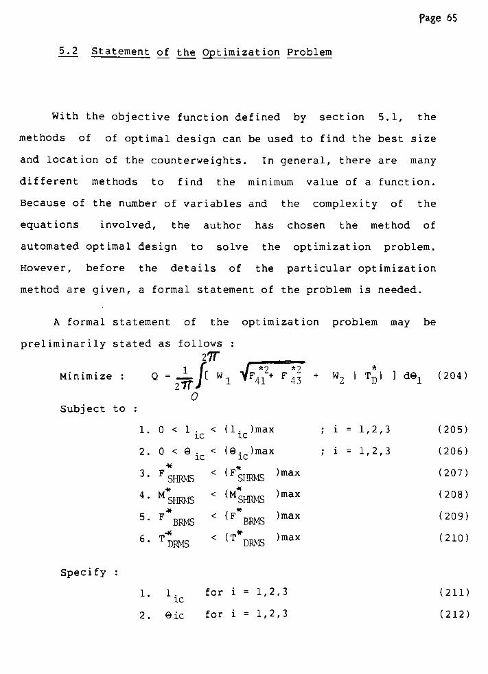
Page 65
5.2 Statement of the Optimization Problem
With the objective function defined by section 5.1, the
methods of of optimal design can be used to find the best size
and location of the counterweights. In general, there are many
different methods to find the minimum value of a function.
Because of the number of variables and the complexity of the
equations involved, the author has chosen the method of
automated optimal design to solve the optimization problem.
However, before the details of the particular optimization
method are given, a formal statement of the problem is needed.
A formal statement of the optimization problem may be
preliminarily stated as follows :
27T
Minimize
Subject to
Q =2"^/[ WlVf4*!2+
?H+
W2 I T*| ] d9, (204)
2
0
1. 0 < 1 .< ( 1 )max
ic ic
2. 0 < 9 -< (9 - )max
ic ic
3' FSHRMS
<
(F!HRMS )maX
4' MSHRMS
< (MSHRMS
)maX
5' F*BRMS<
(F*BRMS )max
6' T^RMS<
(T*DRMS )maX
i = 1,2,3 (205)
i = 1,2,3 (206)
(207)
(208)
(209)
(210)
Specify :
1. 1 .for i = 1,2,3 (211)
ic
2. 9ic for i = 1,2,3 (212)
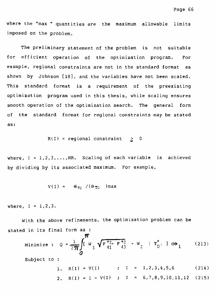
Page 66
where the "max"
quantities are the maximum allowable limits
imposed on the problem.
The preliminary statement of the problem is not suitable
for efficient operation of the optimization program. For
example, regional constraints are not in the standard format as
shown by Johnson [18], and the variables have not been scaled.
This standard format is a requirement of the preexisting
optimization program used in this thesis, while scaling ensures
smooth operation of the optimization search. The general form
of the standard format for regional constraints may be stated
as:
R(I) = regional constraint > 0
where, I = 1,2,3 , . . . ,NR. Scaling of each variable is achieved
by dividing by its associated maximum. For example,
V(I) =
9IC /(9-rc )max
where ,I = 1,2,3.
With the above refinements, the optimization problem can be
stated in its final form as :
n
Minimize: Q =r-fl W.V^
F \\ +W2 |TDl]d9l (213)
0
Subject to :
1. R(I) = V(I) ; I = 1,2,3,4,5,6 (214)
2. R(I) = 1 - V(I) ; I = 6,7,8,9,10,11,12 (215)
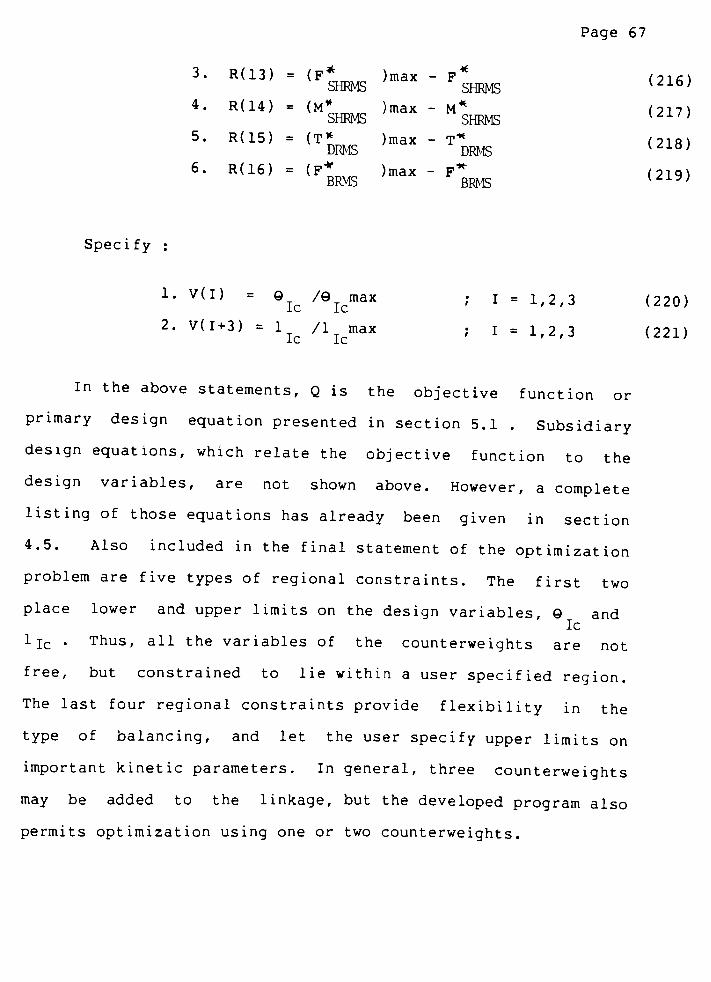
Page 67
3. R(13) =(F*
n)max -
F*
SHRMS SHRiMS
4. R(14) =(M*
^)max -
M*
SHRMS SHRMS
5. R(15) = (T*
DRMS
6. R(16) =(P*
BRMS
{max -
T"*
DRMS
)max -
BRMS
(216)
(217)
(218)
(219)
Specify :
1. V(I) = /9 max
Ic Ic
2. V(I+3) = 1 /l max
Ic Ic
I = 1,2,3
I = 1,2,3
(220)
(221)
In the above statements, Q is the objective function or
primary design equation presented in section 5.1 . Subsidiary
design equations, which relate the objective function to the
design variables, are not shown above. However, a complete
listing of those equations has already been given in section
4.5. Also included in the final statement of the optimization
problem are five types of regional constraints. The first two
place lower and upper limits on the design variables, and
Ic
1 ic . Thus, all the variables of the counterweights are not
free, but constrained to lie within a user specified region.
The last four regional constraints provide flexibility in the
type of balancing, and let the user specify upper limits on
important kinetic parameters. In general, three counterweights
may be added to the linkage, but the developed program also
permits optimization using one or two counterweights.

Page 68
Many automated optimization techniques are available to
solve the above defined problem. Because of its flexibility and
the author's familiarity, the MODSER program developed by
Johnson [18] was used. The author has chosen to rewrite the
existing program in the FORTRAN language, and it is herein
refered as the AOD program. A brief, but informative summary of
the AOD program is given in the next section.
Page 69
5. 3 Summary of the AOD Program
The logic which the AOD program uses to find a solution to
an optimization problem is briefly presented below. The
structure of the program is the same as the MODSER program
developed by Dr R. C. Johnson [18]. The version in this thesis
has been rewritten in the FORTRAN programming language for use on
a VAX/VMS digital computer. When the AOD program is used to
solve the specific problem of balancing four bar linkages, it is
refered to as the OPTBAL program. A complete summary of the
OPTBAL program including input and output is given in appendix D.
Algorithms of automated optimal design basically control an
iterative, computer based search using the techniques of
nonlinear programming. The purpose of the search is to find an
approximate minimum of an objective function, Q, while
maintaining user specified regional and equality constraints.
These constraints are taken into account using a penalty function
, P, which is directly added to the objective function. The
search process in the MODSER program mainly consists of two parts
; determination of a search direction and a univariate line
search. Both parts of the search are repeatedly applied until an
approximate minimum is reached. The specifics of the penalty
function, search process and termination criteria will be
presented next.

Page 70
Many strategies of automated optimal design are based on
minimizing an unconstrained function. Since the balancing
problem has regional constraints, it must be converted into an
equivalent unconstrained optimization problem before it can be
solved. To achieve this, the MODSER program incorporates a
penalty function, P, which is added to the objective function
when constraints are violated. Thus, the search for a minimum
value of the objective function will probably avoid violating
regional constraints since, if it does, the objective function is
increased. The form of the penalty function used in the MODSER
Program maY t>e expressed as :
Ne2
Nr2
P = Cp7?p[ H C Ej ] + l[Ri- iRil 1 ] (222)
j=l 4 i=l
Where Cp is the penalty function coefficient which is
automatically tuned by the AOD program to balance it with respect
to the optimization quantity. 7}p is a factor which is increased
as the solution is approached to emphasize the effect of regional
constraint violations in the search process. Ej is the jth
equality constraint expressed in the form : Ej (x) = 0, where x
is the vector of the independent search variables. Ri is the ith
regional constraint expressed in the form : Ri (x) > 0. To
incorporate the penaltyfunction into the objective function, the
two are simply added to form a new optimization quantity.
Qu= Q + P (223)
Therefore, the regional constraints have been taken into account
by redefining the objective function. Although the problem is to
Page 71
minimize an equivalent unconstrained function, the correct final
solution should show that all of these constraints have been
obeyed. In some situations, the user may specify regional
constraints which are impossible to meet. Such a situation may
still yield a final solution, but the results should not be
considered since constraints have been violated. To alleviate
this problem, regional constraints may be relaxed (ie. open up
the design space), and the optimization rerun.
The basic structure of the MODSER program is shown in Figure
8. Once the problem has been set up in the standard format, the
program may be run. Data is entered into the program through an
external data file as shown in appendix D. After the data has
been read, then a starting point for the search is either
specified or automatically calculated using the random generation
method. Due to the complexity of the balancing problem of this
thesis, starting points were always obtained using the random
number generation method. After a suitable starting point has
been found, the program performs an initialization. The initial
search direction is then found using the method of steepest
descent (MSD) where the search direction vector, s, is just the
negative of the gradient vector, g_. A technique which is more
efficient than MSD, is the generalized conjugate gradient method
(GCG) and may be given as:
-
9+
w, (224)s
-K -K K- K-1
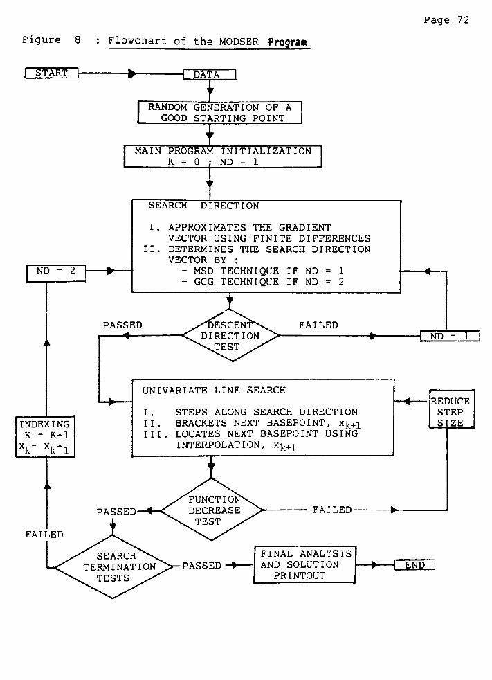
Page 72
Figure 8
j START h
ND = 2
INDEXING
K = K+1
Xk=
Xk+1
FAILED
Flowchart of the MODSER Progran
DATA
RANDOM GENERATION OF A
GOOD STARTING POINT
MAIN PROGRAM INITIALIZATION
K = 0 ND = 1
SEARCH DIRECTION
I. APPROXIMATES THE GRADIENT
VECTOR USING FINITE DIFFERENCES
II. DETERMINES THE SEARCH DIRECTION
VECTOR BY :
- MSD TECHNIQUE IF ND = 1- GCG TECHNIQUE IF ND = 2
PASSED
4
FAILED
UNIVARIATE LINE SEARCH
I. STEPS ALONG SEARCH DIRECTION
II. BRACKETS NEXT BASEPOINT, x^+iIII. LOCATES NEXT BASEPOINT USING
INTERPOLATION, x^+i
-\ ND = 1
IREDUCE
STEP
SIZE _
FINAL ANALYSIS
AND SOLUTION
PRINTOUT
Page 73
where,
WK= ( 9K
"
g<H ) (gK ) (225)
<sk
-eK+1) (sK., )
The subscript k is used to designate the number of iterations.
The QC6 technique requires two consecutive basepoints for its
evaluation and therefore, cannot be used in the initial search
direction determination. Once the search direction has been
found by either of the N|SD or QCG techniques, then a descent
direction test is applied which is given by :
g . s < 0 (226)
The above test is imposed to ensure that the search direction
chosen is one in which the function decreases. If the descent
direction test is passed, then a univariate line search is
carried out along the calculated search direction. The end
result of the line search is an approximate function minimum
along that search direction. This is accomplished by finding
three points within which the minimum exists, and applying an
interpolation technique. After the line search is completed, a
check is made on the new proposed basepoint to see if the
objective function has been lowered. If the test is failed, the
incremental step size is reduced and the unvariate line search
is repeated. If the function decrease test is passed, then a
search termination test is applied. The termination test
consists of three steps: the distance between successive

Page 74
basepoints, the value of 7) p in comparison to 7/pmax, and the
rate of convergence of the solution. If anyone of the above
three tests for convergence are failed, then the new basepoint,
x k+1 is chosen from the results of the line search, the counter,
k is indexed and a new search direction is made. If however,
the termination tests are passed, then the search is halted and
the results are printed out.
Page 75
5.4 Summary of Analysis and Final Subroutines
The AOD computer program presented in the last section
requires a subroutine to evaluate the objective function,
regional constraints and equality constraints. In addition the
program needs a subroutine to print out the final results.
These two tasks are performed by the Analysis and Final
subroutines, which are listed in appendix D for the problem of
balancing four bar linkages (.ie, the OPTBAL program ). A block
diagram showing how information is passed from the OPTBAL main
program to the Analysis and Final subroutines is shown in Figure
9. The"Pgauss"
subroutine, which is also shown in that figure,
provides data for numerical integration using Gaussian
quadrature. The four different components were compiled
separately, and then linked into one executable program.
General comments about each will be presented next, while the
specific options of the OPTBAL program are given in appendix D.
The analysis subroutine, as mentioned earlier, evaluates
the important equations of a particular problem such as :
regional constraints, equality constraints, objective function.
As was shown in section 5.1, the objective function used in the
OPTBAL program must be integrated over the full range of the
input. Due to the complexity of this objective function,
integration was done numerically using either Gaussian
quadrature or a simple summation approach. Appendix C provides
indepth details about each type of numerical integration. Both
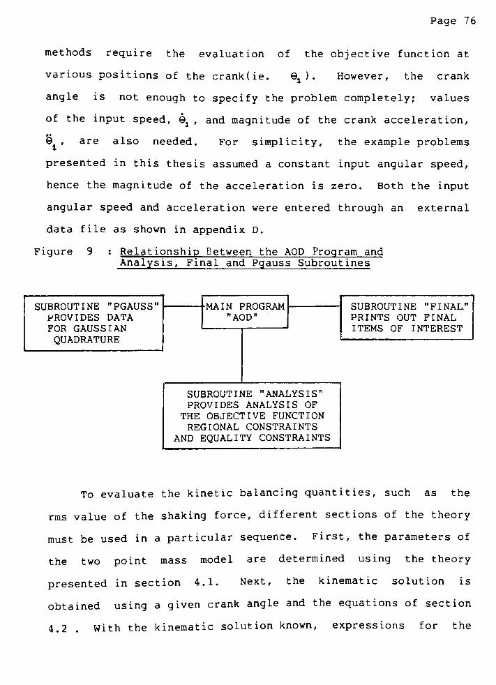
Page 76
methods require the evaluation of the objective function at
various positions of the crank(ie. a ) . However, the crank
angle is not enough to specify the problem completely; values
of the input speed, 9a , and magnitude of the crank acceleration,
9 , are also needed. For simplicity, the example problems
presented in this thesis assumed a constant input angular speed,
hence the magnitude of the acceleration is zero. Both the input
angular speed and acceleration were entered through an external
data file as shown in appendix D.
Figure 9 : Relationship Between the AOD Program and
Analysis, Final and Pgauss Subroutines
SUBROUTINE"PGAUSS"
PROVIDES DATA
FOR GAUSSIAN
QUADRATURE
,U1TH DBOCOIM SUBROUTINE"FINAL"
PRINTS OUT FINAL
ITEMS OF INTEREST
iTIAIIN rKUuKArl
"AOD"
SUBROUTINE"ANALYSIS"
PROVIDES ANALYSIS OF
THE OBJECTIVE FUNCTION
REGIONAL CONSTRAINTS
AND EQUALITY CONSTRAINTS
To evaluate the kinetic balancing quantities, such as the
rms value of the shaking force, different sections of the theory
must be used in a particular sequence. First, the parameters of
the two point mass model are determined using the theory
presented in section 4.1. Next, the kinematic solution is
obtained using a given crank angle and the equations of section
4.2 .With the kinematic solution known, expressions for the
Page 77
bearing forces, input torque, shaking force, shaking moments and
the integrand of the objective function are evaluated
sequentially^ as summarized in section 4.5 . The above two steps
are repeated for various crank angles as determined by the
numerical quadrature. Once this is complete, the objective
function and rms quantities are determined. Finally, the
regional constraints are evaluated^and the objective function
may be modified by a penalty function as shown in section 5.3 .
The two options for numerical integration are Gaussian
quadrature (NRMS = 1), and the simple summation technique (NRMS
= 2). The degree of integration for each type of quadrature can
be changed using an externally specified variable, NGQ. For
Gaussian quadrature, NGQ represents the number of sampling
points, and can range from one to twenty-four. For integration
by simple function summation, the NGQ variable is an indirect
indication of the number of sampling points, and is given by the
following formula.
number of sampling points = 360 / NGQ
The number 360 in the above expression is representative of
the maximum number of sampling points using the simple summation
technique(eg. NGQ =1). At this limit, the quadrature would
require evaluation of the integrand for every degree of the
crank, or 360 times per cycle. As will be shown in example one,
proper choice of NGQ for each type of quadrature will produce
analysis results which converge. The Gaussian quadrature is
Page 78
also available since it provides a relatively efficient form of
integration. However, this type of quadrature is incapable of
accurately predicting maximum quantities. This is acceptable
for a large part of the optimization since the regional
constraints and objective function are based upon rms quantities.
However, for the final design it is desirable to know the
maximum values of some quantities. For example, the maximum
input torque should be known in order to select a motor for the
linkage. For this reason, the the OPTBAL program uses simple
summation integration to analyze the final results.
In addition to the Analysis subroutine, the user of the AOD
program must also supply a Final subroutine to print out the
results of the optimization. For the OPTBAL program, the output
includes a summary of the actual dimensions and angular
locations of the counterweights. A listing of the regional
constraints and values of the bearing forces, shaking force,
shaking moment and input torque are also provided. The
optimization search is also summarized through yet another data
file.
As a whole the OPTBAL program offers several important
features. For instance, the user can select the number of
counterweights to be added. By adjusting the number of
counterweights, NC, the effects of adding from one to three
counterweights can be evaluated through a series of optimization
runs. In addition, the choice of no counterweights
(NC=0) , allows the user to analyze the unbalanced linkage. As

Page 79
shown in appendix D, the only limit of the NC option is the
location of the counterweights. The effects of changing the
number of added counterweights is investigated in examples 2 and
3. Another feature of the program is that it allows the user to
select the maximum regional constraint parameters on the rms
values of important kinetic quantities, such as the shaking
force or input torque. Regional constraint limits can be easily
changed through the input data file and permits diversity in
balancing. Investigation of the regional constraint variations
are shown in example 1.
Page 80
6.0 PRESENTATION OF EXAMPLE PROBLEMS
The capabilities, and effectiveness of the developed
balancing program, OPTBAL, will now be demonstrated through some
example problems. These example problems were taken from other
published sources and provide comparisons to the unbalanced
linkage, as well as other methods of balancing. A brief
description of each will be presented in the next several pages,
while the details and results are shown in sections 6.1 through
6.3 .
The three example problems presented are ;
Example 1 : Capabilities of the OPTBAL Program
Example one provides some insight into the capabilities of
the OPTBAL program. In the first portion, a comparison is
made between the two types of numerical integration
available in the program. For simplicity, the comparison
is made using an unbalanced inline four bar linkage taken
from Berkoff [5]. From that comparison, the optimum number
of sampling points for a convergent , but efficient
solution is determined. The second part of the problem
focuses on the effect of varying the weighting factors, W^
and W0, upon the optimization results. The effect of
varying the torque regional constraint upon the
optimization results is also shown.
Page 81
Example 2 : Balancing of an Inline Four Bar Linkage
The results of example one are applied to balance the four
bar linkage of that example in a typical design procedure.
The effects of varying the number of added counterweights
is shown. The results of the optimization are then
compared to the unbalanced linkage, the completely force
balanced linkage, and the complete force and moment
balanced linkage.
Example 3 : Balancing of a Four Bar Linkage with
an Offline Coupler Mass
In this example, a graphical comparison between the method
of complete force balancing, and the method of balancing
linkages using the OPTBAL program is made. The linkage has
been taken from Tricamo and Lowen [40], and contains a
coupler link with an offline center of mass. The procedure
for balancing is the same as that in example 2 since, the
number of added counterweights are varied. The most
practical counterweight design will then be compared
graphically to the unbalanced, and completely force
balanced linkage.
The full details of each of the three examples will be
presented next in sections 6.1 through 6.3 .
Page 82
6.1 Capabilities of the OPTBAL Computer Program
In this example, the capabilities of the OPTBAL program
are investigated . The information gained will provide
insight as to the selection of several OPTBAL parameters for
an accurate^nd efficient analysis. In addition, limitations
of the regional constraints will be demonstrated.
A typical inline four bar linkage, taken from Berkoff
[5], will be used to show these capabilities. The linkage is
shown in Figure 10 and its specifications are given in Table
1. The linkage and counterweights are assumed to be made out
3
of steel with a density of 0.283 (lb/in ). The counterweights
are also assumed to be circular and have a constant thickness
of 0.50 inches. Counterweights may be tangentially attached
to joints 0., O, or 03 ,as shown in Figure 1 of section 4.1.
The input speed of the linkage is assumed to be constant at
5000 rpm (523 rad/s) .
The first part of this example compares the two different
types of numerical integration available in the OPTBAL
program: Gaussian quadrature, simple summation quadrature.
Integration is used by the program to evaluate the objective
function and other rms quantities. Therefore, the degree of
numerical integration used is important in providing an
accurate analysis. So, from an accuracy point of view, we

Figure 10 : Inline Four Bar Linkage
Page 83
L:
0.50),
A
0.50"R
lz <D
<Z>L
L-
TTTTTT7T
0.50R
^-H
O;
0.50 R
// / / n / / / 1 1) i > h
U
1
V ^
Table 1 : Parameters of the Unbalanced Inline Four Bar Linkage
Link No . ,i 1 2 3 4
Length, Li (in) 1.000 4.000 3.000 3.000
Mass, mi (lb) 0.101 0.174 0.146 -
Length to C.G.
Location, li (in) 0.500 2.000 1.500 -
Thickness ( in) 0.200 0.200 0.200 -
Mass Moment of Inertia
about the C.G. Location
I? (lb - in2)
0.036 0.433 0.232 -
Page 84
might consider using a relatively high order of numerical
quadrature (ie. a large number of sampling points). On the
other hand, it is desirable to minimize the number of function
evaluations required in each analysis subroutine. If the
number of function evaluations are too large, then an
excessive amount of computer time will be used. This part of
example one will determine which degree of numerical
integration is best suited for an efficient .but accurate
analysis.
To achieve this goal, the number of sampling points, NGQ,
was varied while setting the number of counterweights option^
NC, to zero. This, in effect, enabled the optimization
program to analyze the unbalanced linkage. For each trial,
the rms values of the normalized shaking force, shaking moment
and input torque were recorded. A plot of this data is shown
in Figures 11, 12 and 13. As can be seen from those figures,
both types of integration converge to the same solution, with
the Gaussian quadrature being slightly more efficient. It
appears that NGQ must be greater than 10 for an accurate
analysis using Gaussian quadrature, while NGQ must be greater
than 15 for the simple summation quadrature. From an
efficiency standpoint, the Gaussian quadrature, as expected,
is better (approximately 33 %). Therefore, the remaining
example problems will use Gaussian quadrature as the method of
numerical integration, with the number of sampling points
equal to 10.

Page 85
tnI-
T oj
o
o.
o
_ co
<r
tn
u.
o
a:
ui
co
tn
UJZ>
or)
l-HO
Li_Q
o
CD
a:
ui
o
UJ z
Qi O
t-ZIi-
<ro:z>
Qii-U
Qf-O
<r <xcn
IDE
ID2I
ZCOUI
<r <3
iluq:
tn_JUJCOQ_Z>
ZDSIZ
<THO
ocno
< a I
< a
4I
I
to
T
D**
I
D j<l
a <j
<
a <
a
id
r-
k>
_ cu
<s>
-
CO
-
to
(Si
O
Q_
O
(Si
UI
CO
OJ
<S>
2r o ore <r i -4 csj uj o or: :coHZQ-Df- f-OQOZ)UJ

Page 86
tn
o
<3
tn
OT
ui
co
oj ?
^cn
z>
UJ
OrTUJ
Z>0
oo:
HO
U_ LL
CS
<r
X
tn
tn
or
a
UJ
Ni
_j
<r
or
o
lo
LT>
uj z:
or o
HZf-
<tozdort
_j
oe-o
<x<rtn
DEOSZE-
DZ
ZO)UJ
<r o
uj or
tn-Jui
tno_z>
ideiz:
<lHO
0(/)0
< D I
< ?
T
i
? <!
i
d < ;
ru
_ co
_ to
_ ru
_<s>
co
-
to
tn
o
Q_
<3
to
O
or
LU
CO
<
<
ru
Lf) LO LO ro LO
OJ
s>
OJ
z:oorsr<u-([sjLiJO or e: co i/>i<i.^h: o U.OOTOUJ
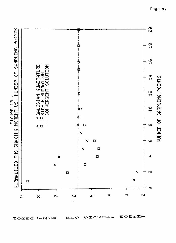
Page 87
tn
O
O
<r
to
o
or
UJ
co
to
oUJ
o
<r
tn
to
sr
or
Q
ui
N
or
o
or o
Z) -
f-ZH
<XOZ)
or-_i
QhO
<cozto
zieOEIH-
ZJZT
ZCOUl
<I C5< uior
cnjlu
too_r>
<lHO
otoo
< D i
< D
CD CO
D
F
9i
I
JoI
<
a
?
D
ru
_ co
_ to
_rr
_ oj
_<s
CO
-
to
T
OJ
CO
r-
LO
to
O
Q_
o
to
or
ui
co
z>
<s>
cn OJ
ZOttECJHNUP OTECO ^KL^'mZOEOS.UJZ.I-
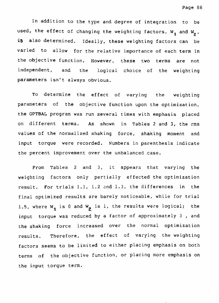
Page 88
In addition to the type and degree of integration to be
used, the effect of changing the weighting factors, W, and W,
15 also determined. Ideally, these weighting factors can be
varied to allow for the relative importance of each term in
the objective function. However, these two terms are not
independent, and the logical choice of the weighting
parameters isn't always obvious.
To determine the effect of varying the weighting
parameters of the objective function upon the optimization,
the OPTBAL program was run several times with emphasis placed
on different terms. As shown in Tables 2 and 3, the rms
values of the normalized shaking force, shaking moment and
input torque were recorded. Numbers in parenthesis indicate
the percent improvement over the unbalanced case.
From Tables 2 and 3, it appears that varying the
weighting factors only partially effected the optimization
result. For trials 1.1, 1.2 and 1.3, the differences in the
final optimized results are barely noticeable, while for trial
1.5, where W is 0 and W is 1, the results were logical; the
input torque was reduced by a factor of approximately 3 , and
the shaking force increased over the normal optimization
results. Therefore, the effect of varying the weighting
factors seems to be limited to either placing emphasis on both
terms of the objective function, or placing more emphasis on
the input torque term.
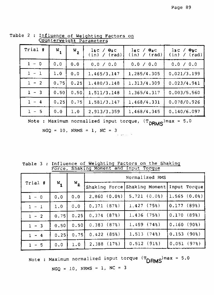
Page 89
Table 2 : Influence of Weighting Factors on
Counterweight Parameters
Trial ft Wl WE lie / 9a c
(in) / (rad)
lzc / 9ac
(in) / (rad)
l3C / 93C
(in) / (rad)
1-0 0.0 0.0 0.0 / 0.0 0.0 / 0.0 0.0 / 0.0
1-1 1.0 0.0 1.465/3.147 1.285/4.305 0.021/3.199
1-2 0.75 0.25 1.480/3.148 1.313/4.309 0.023/4.941
1-3 0.50 0.50 1.511/3.148 1.365/4.317 0.003/5.560
1-4 0.25 0.75 1.581/3.147 1.468/4.331 0.078/0.926
1-5 0.0 1.0 2.913/3.359 1.468/4.345 0.140/6.097
Note : Maximum normalized input torque, (T_.p. *c;)max = 5.0
NGQ = 10, NRMS = 1, NC = 3
Table 3 : Influence of Weighting Factors on the Shaking
Force, Shaking Moment and Input Torque
Trial # Wl WZ
Normalized RMS
Shaking Force Shaking Moment Input Torque
1-0 0.0 0.0 2.860 (0.0%) 5.721 (0.0%) 1.565 (0.0%)
1-1 1.0 0.0 0.371 (87%) 1.427 (75%) 0.177 (89%)
1-2 0.75 0.25 0.374 (87%) 1.436 (75%) 0.170 (89%)
1-3 0.50 0.50 0.383 (87%) 1.459 (74%) 0.160 (90%)
1-4 0.25 0.75 0.422 (85%) 1.513 (74%) 0.153 (90%)
1-5 0.0 1.0 2.388 (17%) 0.512 (91%) 0.051 (97%)
Note : Maximum normalized input torque
(T^,Jmax =5.0
NGQ = 10, NRMS = 1, NC = 3
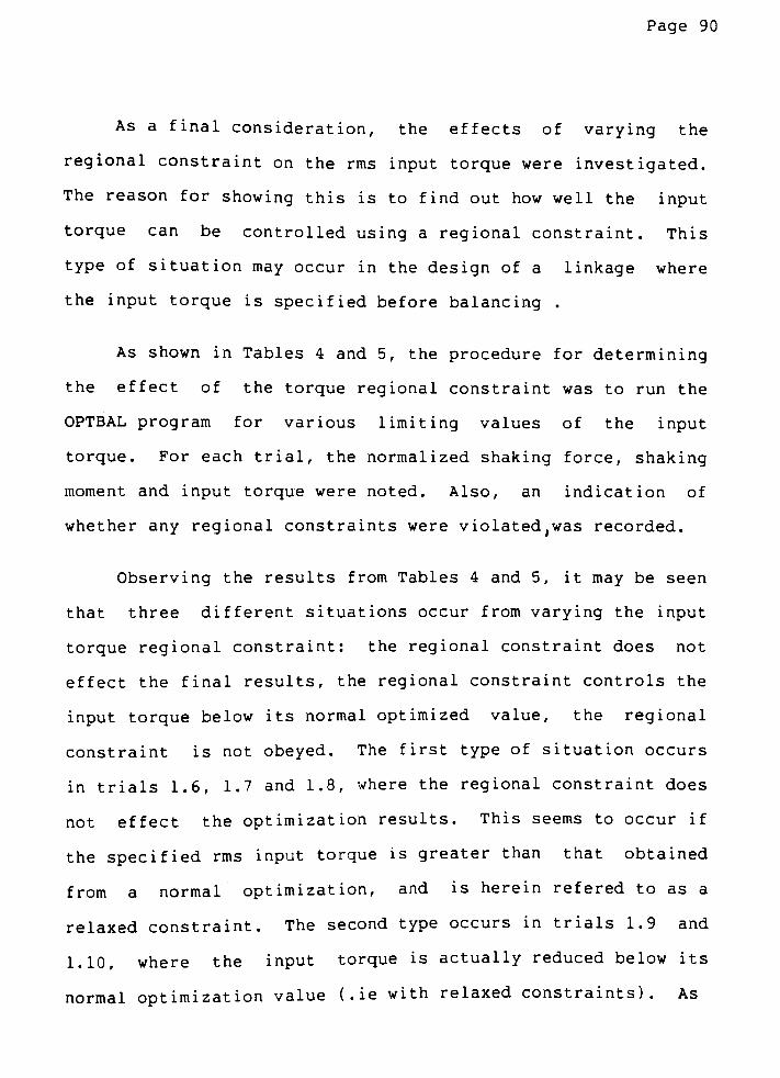
Page 90
As a final consideration, the effects of varying the
regional constraint on the rms input torque were investigated.
The reason for showing this is to find out how well the input
torque can be controlled using a regional constraint. This
type of situation may occur in the design of a linkage where
the input torque is specified before balancing .
As shown in Tables 4 and 5, the procedure for determining
the effect of the torque regional constraint was to run the
OPTBAL program for various limiting values of the input
torque. For each trial, the normalized shaking force, shaking
moment and input torque were noted. Also, an indication of
whether any regional constraints were violated,was recorded.
Observing the results from Tables 4 and 5, it may be seen
that three different situations occur from varying the input
torque regional constraint: the regional constraint does not
effect the final results, the regional constraint controls the
input torque below its normal optimized value, the regional
constraint is not obeyed. The first type of situation occurs
in trials 1.6, 1.7 and 1.8, where the regional constraint does
not effect the optimization results. This seems to occur if
the specified rms input torque is greater than that obtained
from a normal optimization, and is herein refered to as a
relaxed constraint. The second type occurs in trials 1.9 and
1.10, where the input torque is actually reduced below its
normal optimization value ( . ie with relaxed constraints). As
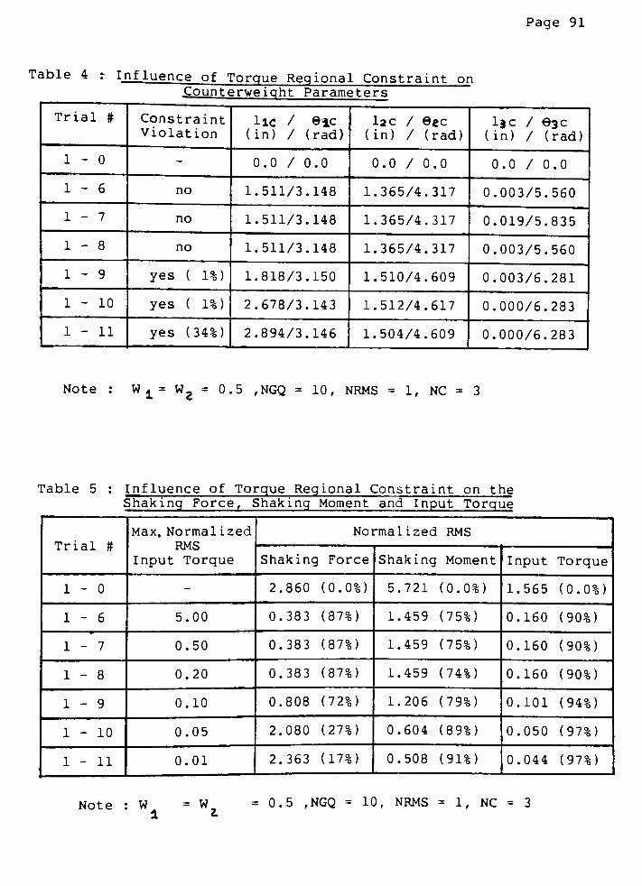
Page 91
Table 4 r Influence of Torque Regional Constraint on
Counterweight Parameters
Trial # Constraint
Violationlie / ic
(in) / (rad)
l2C / 9gc
(in) / (rad)
lac / 93c
(in) / (rad)
1-0 -
0.0 / 0.0 0.0 / 0.0 0.0 / 0.0
1-6 no 1.511/3.148 1.365/4.317 0.003/5.560
1-7 no 1.511/3.148 1.365/4.317 0.019/5.835
1-8 no 1.511/3.148 1.365/4.317 0.003/5.560
1-9 yes ( 1%) 1.818/3.150 1.510/4.609 0.003/6.281
1-10 yes ( 1%) 2.678/3.143 1.512/4.617 0.000/6.283
1-11 yes (34%) 2.894/3.146 1.504/4.609 0.000/6.283
Note : W1=
W2= 0.5 ,NGQ
= 10, NRMS = 1, NC = 3
Table 5 : Influence of Torque Regional Constraint on the
Shaking Force, Shaking Moment and Input Torque
Trial #
Max. Normalized
RMS
Input Torque
Normalized RMS
Shaking Force Shaking Moment Input Torque
1-0 - 2.860 (0.0%) 5.721 (0.0%) 1.565 (0.0%)
1-6 5.00 0.383 (87%) 1.459 (75%) 0.160 (90%)
1-7 0.50 0.383 (87%) 1.459 (75%) 0.160 (90%)
1-8 0.20 0.383 (87%) 1.459 (74%) 0.160 (90%)
1-9 0.10 0.808 (72%) 1.206 (79%) 0.101 (94%)
1-10 0.05 2.080 (27%) 0.604 (89%) 0.050 (97%)
1-11 0.01 2.363 (17%) 0.508 (91%) 0.044 (97%)
Note : W = W =0.5 ,NGQ
= 10, NRMS = 1, NC = 3
Page 92
noted from the results, some regional constraints have been
violated, but the violations are very small in comparison to the
input torques value. The last type occurs when the constraints
on the input torque-are virtually impossible to meet, and the
regional constraint is significantly violated. This occurred in
trial 1.11 and is commonly refered to as a case of incompatible
specif ications( ie. the specifications are impossible
to meet ) .
The results of the second and third portions of example one
appear to show that the amount of reduction of the input torque
can be varied from its normal optimization value (ie. where the
weighting factors are equal and the regional constraints are
relaxed). However, the price for a greater reduction of the
input torque is an increased shaking force. For example, in
trial 1.3, a normal optimization decreased the shaking force by
approximately 87% and reduced the input torque by 90%. However,
in trial 1.5,where more emphasis was placed on the input torque
reduction, the input torque was decreased 97% and the shaking
force reduced by only 17% over the unbalanced linkage.
Therefore, trial 1.5 increased the shaking force 70% over the
normal optimization results, while the input torque was only
reduced an additional 7%. In otherwords, the price of putting
emphasis on the input torque seems to adversely effect the other
balancing parameters. Since the main objective of this thesis
is to reduce the combined effects, the remainder of the example
problems will use equal weighting factors and relaxed regional
constraints.

Page 93
6. 2 Balancing of an Inline Four Bar Linkage
The objective of this example problem is to specify
counterweights for the inline four bar linkage of example one, so
that the combined effects of the shaking force, shaking moment,
bearing forces and input torque are balanced. The purpose of
this example problem is to show a practical procedure for
applying the OPTBAL program . In addition, this example will
provide comparisons to other balancing methods such as the method
of complete force balancing, and complete force and moment
balancing.
The balancing procedure consists of varying the number of
counterweights to be added to the linkage. The OPTBAL program
was run for each of the three possible counterweight
configurations with the regional constraints relaxed, and the
weighting factors selected equal to each other.
Results for each one of the trials are shown in tables 6, 7
and 8. Table 6 shows the specifications of the counterweights,
while Tables 7 and 8 list the rms and maximum dynamic quantities
for each trial respectively. Numbers in parenthesis in these
tables indicate the percent improvement over the unbalanced case.
Trials 1.0, 2.4 and 2.5 have been included in each of the three
tables for comparison purposes. Trial 1.0 is the unbalanced
linkage, while trials 2.4 and 2.5 were obtained from Berkoffs
paper [5].Trial 2.4 is the complete force balanced linkage, and
trial 2.5 is the complete force and moment balanced linkage.

Page 94
Table 6 : Counterweight Parameters for Example 2CD
Trial # NC lie / 9-j.c
(in)/(rad)
lzc / 92c
(in)/(rad)
lie / 93C
(in)/(rad)
Ref .
1-0 0 0.0 / 0.0 0.0 / 0.0 0.0 / 0.0 unbalanced
2-1 1 1.299/3.062 0.0 / 0.0 0.0 / 0.0 OPTBAL
2-2 2 1.299/3.062 0.0 / 0.0 0.036/0.277 OPTBAL
2-3 3 1.511/3.148 1.365/4.317 0.003/5.560 OPTBAL
2-4 2 0.717/3.142 0.0 / 0.0 1.079/3.142Ref.[5]C2)
2-5 2 0.717/3.142 0.0 / 0.0 1.079/3.142Ref.[5](3)
Note : (1) OPTBAL options used : NRMS=1 ,NGQ=10 ,Wl=Wa=0 . 5
<TDRMSW5-0
(2) Force balanced.
(3) Force and moment balanced . In addition to two
circular counterweights, geared inertia
counterweights have been added, and the shape
of the coupler link has been augmented.
As can be seen from the results tables, the linkages
balanced using the OPTBAL program are superior to those of the
unbalanced, completely force balanced, and completely force and
moment balanced linkages . The ranges of all force and moment
reductions for the linkages balancedby the OPTBAL program are on
the order 75 % to 92 % over the unbalanced linkage. In contrast,
the completely force balanced linkage eliminated the shaking
force, but increased all other balancing quantities over the
unbalanced linkage. The situation is even worse for the
completely force and moment balanced linkage. Although both the

Page 95
Table 7 : Comparison of Normalized RMS Quantities for
Example 2
Kinetic
Quantity
Trial #
1-0 2-1 2-2 2-3 2-4 2-5
p*
SH2.860
(0.0%)
0.620
(78%)
0.620
(78%)
0.383
(87%)
0.0
(100%)
0.0
(100%)
M*
,
SH/015.721
(0.0%)
1.440
(75%)
1.440
(75%)
1.459
(74%)
7.610
(-33%)
0.0
(100%)
m -k
D
1.565
(0.0%)
0.394
(75%)
0.394
(75%)
0.160
(90%)
2.467
(-58%)
6.154
(-293%)
F*
21
3.434
(0.0%)
0.864
(75%)
0.864
(75%)
1.197
(65%)
5.271
(-53%)
6.434
(-874)
p*
32
2.380
(0.0%)
0.599
(75%)
0.599
(75%)
0.543
(77%)
4.022
(-69%)
5.066
(-113%)
p*
41
3.801
(0.0%)
0.664
(82%)
0.664
(82%)
0.297
(92%)
4.583
(-20%)
5.734
(-51%)
p*
43
2.299
(0.0%)
0.579
(75%)
0.579
(75%)
0.547
(76%)
4.583
(-99%)
5.734
(-149%)
Table 8 : Comparison of Normalized Maximum Quantities
for Example 2
Kinetic
Quantity
Trial ft
1-0 2-1 2-2 2-3 2-4 2-5
p*
SH
5.572
(0.0%)
1.212
(78%)
1.212
(78%)
0.745
(87%)
0.0
(100%)
0.0
(100%)
M*
.
SH/01
14.68
(0.0%)
3.695
(75%)
3.695
(75%)
3.124
(79%)
17.66
(-20%)
0.0
(100%)
*
TD4.485
(0.0%)
1.129
(75%)
1.129
(75%)
0.405
(91%)
7.092
(-58%)
17.73
(-295%)
p*
21
8.407
(0.0%)
2.116
(75%)
2.116
(75%)
1.850
(78%)
12.89
(-53%)
16.11
(-92%)
*
F326.463
(0.0%)
1.627
(76%)
1.627
(76%)
1.272
(81%)
10.85
(-63%)
13.54
(-104%)
F*
41
8,881
(0.0%)
1.387
(84%)
1.387
(84%)
0.793
(91%)
12.11
(-36%)
15.09
(-70%)
F *
43
6.093
(0.0%)
1.534
(75%)
1.534
(75%)
1.198
(80%)
12.11
(-99%)
15.09
(-148%)

Page 96
shaking force and moment have been eliminated, the remainder of
the balancing quantities have been increased from 70 % to 295 %.
In addition, the completely force and moment balanced linkage
requires large, geared, inertia counterweights to be added to the
input and output shafts, as well as circular counterweights.
Page 97
6.3 Balancing of a Four Bar Linkage
with an Offline Coupler Link
The purpose of this example is to balance a linkage
containing an offline mass distribution. The mechanism was
taken from Tricamo and Lowen [40] and is shown in Figure 14.
As in example two, the counterweights are assumed to be made
out of steel with a density of 0.283 lb/in, and have a
constant thickness of 0.625 inches. The linkage is also
assumed to operate at a constant input speed of 500 rpm (52.3
rad/s) . Counterweights are circular and can be attached
tangentially to joints 0', 0 ,or 0'. Other specifications
for the linkage are given in Table 9.
The procedure for balancing is the same as that in
example 2; the number of counterweights are varied through a
series of optimization trials. The data file for this problem
must, however, take into account the offline placement of the
center of mass of the coupler link (see appendix D) . From
these trials, the most practical scheme for balancing will be
graphically compared to the unbalanced, and completely force
balanced linkages.
The results of this example can be seen in Tables 10 and
11, or graphically in Figures 15 through 22. Specifications
of the counterweights for each trial are given in Table 10,

Page 98
Figure 14 : Four Bar Linkage with an Offline Coupler
nn in
Table 9 : Parameters of the Unbalanced Four Bar Linkagewith an Offline Coupler Link
Link ft, i 1 2 3 4
Length, Li (in) 2.000 6.000 3.000 5.500
Mass, mi (lb) 0.197 0.528 0.268 -
Thickness (in) 0.250 0.250 0.250 -
Length to C.G. , li ( in) 1.000 3.027 1.500 -
Angle,& i (rad) 0.000 0.133 0.000 -
Mass Moment of Inertia
about C.G. Location
lj (lb - in2)
0.146 2.323 0.752 -

Page 99
Table 10 : Counterweight Parameters for Example 3
Trial NC lie / 9ic lac / 9a c 13C / 93C Ref
3-1 0 0.0 / 0.0 0.0 / 0.0 0.0 / 0.0 Unbalanced
3-2 1 1.534/3.088 0.0 / 0.0 0.0 / 0.0 OPTBALfl)
3-3 2 1.534/3.088 0.0 / 0.0 0.031/0.236 OPTBAL( * '
3-4 3 1.958/3.318 1.483/4.239 0.166/6.158 OPTBALf l }
3-5 2 1.095/3.046 0.0 / 0.0 1.292/3.231 Ref[4]C2)
Note :
(1) OPTBAL options used : NRMS=1, NGQ=10, W,=W2=0.5
, , (TDRMS )max = 5-
(2) Force Balanced
Table 11 : Comparison of Normalized RMS Quantities for
Example 3
Kinetic
Quantity
Trial ft
3-1 3-2 3-3 3-4 3-5
F*
SH
3.917
(0.0%)
0.445
(89%)
0.445
(89%)
0.230
(94%)
0.0
(100%)
M*
SH/01
6.866
(0.0%)
0.900
(87%)
0.900
(87%)
0.732
(89%)
1.339
(80%)
M*
i
SH/03
5.427
(0.0%)
0.877
(84%)
0.877
(84%)
0.349
(94%)
1.338
(75%)
TD*
1.992
(0.0%)
0.261
(87%)
0.261
(87%)
0.106
(95%)
0.716
(64%)
p*
21
5.568
(0.0%)
0.730
(87%)
0.730
(87%)
0.899
(84%)
1.975
(64%)
p*
32
3.969
(0.0%)
0.520
(87%)
0.520
(87%)
0.369
(91%)
1.600
(60%)
F*
41
5.889
(0.0%)
0.596
(90%)
0.596
(90%)
0.244
(96%)
1.820
(69%)
p*
43
3.896
(0.0%)
0.511
(87%)
0.511
(87%)
0.372
(90%)
1.820
(53%)
Page 100
while rms values for important dynamic balancing quantities
are shown in Table 11. Trial 3.2 was balanced by the OPTBAL
program with one counterweight attached to the crank. For
this case, all the balancing quantities were reduced from 84 %
to 90 % over the unbalanced linkage. The effect of placing
additional counterweights on the coupler and follower links
can be seen in trials 3.3 and 3.4 . From these trials, it is
evident that the effect of the additional counterweights are
not significant; the reductions only increase 2% to 10% over
the case of adding one counterweight to the crank. From a
practical point of view, this small amount of reduction may
not be worth the trouble of adding a counterweight to both
the coupler and the follower links. Therefore, the case of
adding one counterweight to the crank, trial 3.2, is the
recommended solution to the balancing problem. A comparison
of the important kinetic parameters for the recommended
linkage design, unbalanced linkage and completely force
balanced linkage are shown graphically in Figures 15 through
22. From these graphs, the relative amount of imbalance
between the three linkages can be seen. More importantly, the
graphs give a feeling for the rate of change of the kinetic
quantities over one cycle of the linkage.

Page 101
z
<x
or
o
to
z>
cn
or
ui
in'
o^>
o
or
o
Q
UI
CM
or
o
x
E-*
- %
I ^*LOii
1 Ll t i
or c; I
UJ iF i i
T"
1 1
Z), i
o ' io
\r-y-
i t
LlJ :i
z1 1
oi
o :i
11 ;iU-) i '
ZD :i
-J i
<T1 1
aa i
E \TT-
Q 0_ \ 1 1
UI O \ .1
O \ll
z \ HQ<r CO \ t
UlJ \ 1O Xo Xzco UI \ i:<I o
_JUj i:<EO <x i
COOT_ i;ZO OI t i
1 1 . ro 1 *l
Ii
1
./
1 !;i:t
"i
<
/
*'
/
(
to
n
in
ro
r-
OJ
LO
OJ
OJ
<*v
CT
LO
to
UI
UI
or
C5
O Ct
CO *
UI
z
LO ^
ro . .
<r
or
o
<s>
o
OJ
CO to ru o oo co nj <s>
ZOCtZC JmNUQ U-OOTOUJ *-<z tohzh o^
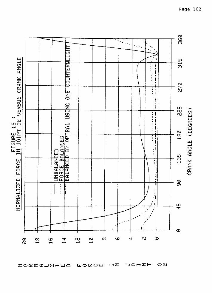
Page 102
o
<E
Z
or
or
o
to
Z)
to
or
ui
z>
OJ
coo
UIZ
or i
ZDO
o
or
o
lo
ci
LU
or
o
F
X
o1 1
LU
*
_
\
^A 1
or
LUF-
3o I
: ii
: i
'. i< i
1i
LU
o
o
z
<r-
1 i
: i
: i: i
tt
tn
Zl
or
COr
: i
: ii
: i
Q
UI
O
z
UI.-J
c-xct
CL
o
CO \B UI
o
-ZL
<r-j
<c
to
\ ii
ii
Ii
1
,/
j
~: *
(
A I
/
1
o
co
cn
LO
ro
<s>
r-
ru
LO
ru
ru
<s>
CO
Ln
cn
<s>
cr>
LO
tn
ui
ui
or
o
ui
o
o;
z
<L
or
o
<s>
o
ru
CO to ru o oo CO oj
zoaE<rJNwUQ u-ooroui nonzh oru

Page 103
LU
_J
O
z
<L
Z
<r
or
<_>
cn
_j
to
or
ui
cn
r-or-\
t
LUZ
or t
zo
o
or
o
o
LU
M
or
O
*
-,.\
s~ -"'-.^ s.
z-^**vfo
h1 't
LU 11
A
or ; \LU i
*
F-\ I
^
. i
z5 \ ', 1o \ '
'
r -i \ ,
lU
V
yA
o 'A
C5i l
Z i
?1?
i-O Iz
i
-J
i
o:i
CO'
t
Cl Q_ t /LU C1
O 7
Z '_-
/ iQ<E CO / '
LU.-J / ic -> <rr o / '
Z CO LU
OI O / >'
_]LU/ 41 t
or o <r / 1COOT _)
\
zo o: XZDU_ CO
Lm
11
1 i \ 11
J
\ ,1
^? 1*
t
_
-
'
'
/
-
i (
<s>
to
cn
LO
cn
OJ
LO
OJ
OJ
CO
in
s>
cn
LO
CO
LU
LU
or
o
LU
Q
LU
_1
o
z
o:
^:
z
o:
or
o
CO to OJ OJ co OJ
z o o_ z -i 3 C 1 UI Cj u_ o or o i z iohzh o ro
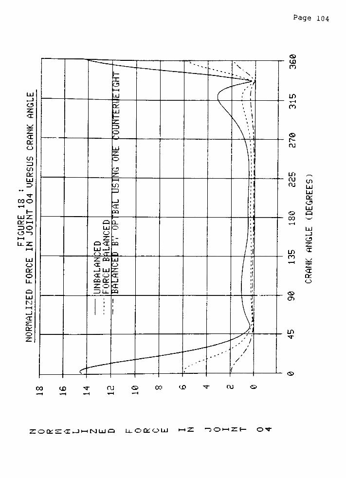
Page 104
<3
Z
OI
\d
z
or.
or
o
to
Zl
to
or
LU
z>
??
coo
uizor
zo
o-D
o
or
o
Q
LU
DnIt i
_1
<z
z
or
o
^
**... \
i-
**
..\
X"
-
s
fC5
>i1
LU ; /
" '
a: ', >LU .
>
s. \ \
z \ **
z> \ ',oI'
1 \ i
LU Vz \ '
i
o
CJ 1z j1 ( j
-*
LO jz
|_)
,
o:|CO
r IF |
o Q_ t
o
io 1zco UJ / !<r o /_JLU Zoio or
COOT -j
zo or
ZJU. PQ
1I
1
/,
*i
/
(
to
ro
in
cn
r-
OJ
L0
OJ
OJ
00
LO
ro
CT)
LO
to
or
o
or
oi
or
o
co co ru co to ru
zoor zoi-Jtinuiq u-ooroi-T)OhhZ{ O'

Page 105
a
LU
or
3'
UI-J
o
z<E
<r
ac
o
cn
z>
to
or
UJz>
'UIo
or
'o
^>
<E
X
cn
Q
UJ
Nl-H
_I
<E
e:
or
o
t-
X
ot 1
UI
r- "
)
//
/1
3
or
UI
z
=3
O
1t
\
\1
\
UI
z
o
o
11
to
Zl
-J
<I
cat-
Q_
O
>
CO
1
*1
UJ
o
z
-J
<E
1i
1
/r
V
to
ro
LO
cn
ru
LT> ^
ruto
LU
UI
or
CJ
LU<s> Q
00 >?
*-t
LUJ
O
z
LO<r
^
z.<r
or
o
<S>
CD
LO
<S>
cn oo CO LO m ru
zoor sajHNiijQ (/,i<iyHzo uooroui
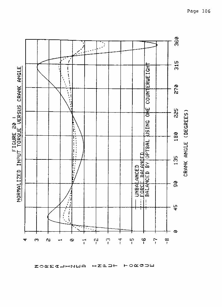
Page 106
LU?J
z
OI
z
<Eor
o
cn
3
to
orLU
or3
o
LU
3o
or
t
Q
LU
N
a:
o
*
J
f
1
t 11
I'
1
\ I*
X
1t
LU
or
LU
\\ < '
\ 1
\ t
Z3
O
o
LU
l\
1 \ll \'. \1 1 \
o
o
z1t
cn
3
i \
< / c
?J
<t
COe-
Q_
O
''
/* /i /
# /
,
z
0<ILU_
0<Lzee
<X
>
CO
LU
O-7-
// 1
t 1
/ "
/ ''
4
(
arc
MCE
ZC
3U
i
_J
<r
CO
1
1
/'
'1
/
\
i 1
CO
ro
in
cn
csr-
OJ
LO SS
OJ (0(U
LULU
or
<J
LU
Q
00S^>
v-t
LU
J
O
z
LO<r
ro^
z
<r
or
o
O
cn
LO
T
cn ru OJ ro
i
LO
i
CO 00
I
Z O Or Z <E _I-N UI Qt-tZQ_3f f O QT O 3 I
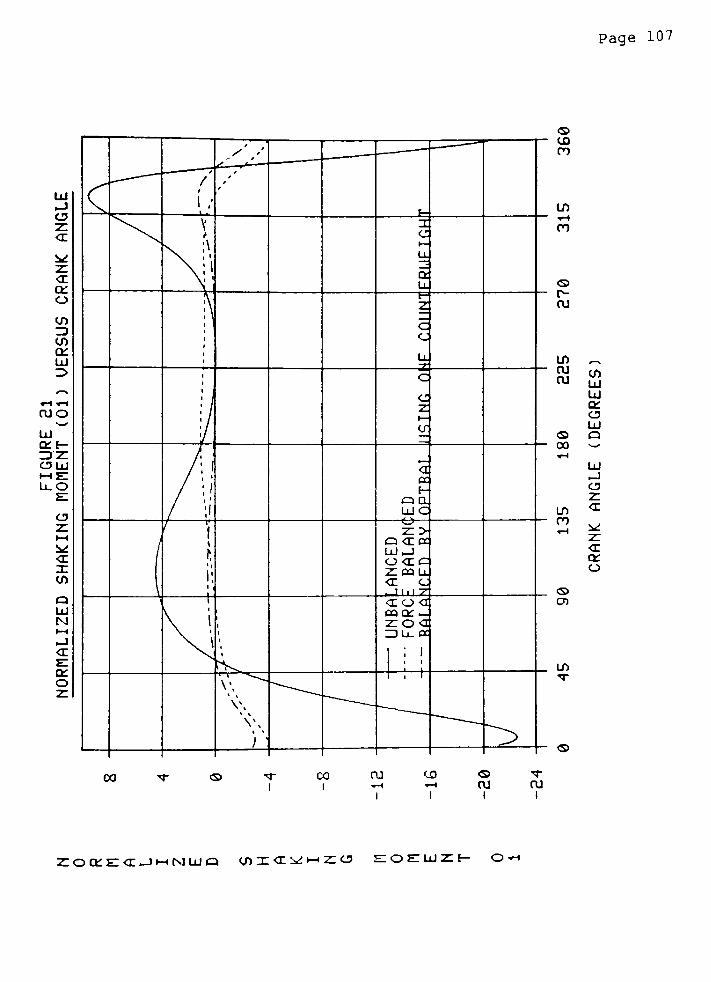
Page 107
o
z
<x
z
<E
or
o
to
3
to
or
UJ
z>
OJO"w*
LUore-
3Z
C3LUt-iZ
UO
O
<E
X
cn
Q
UI
N
or
o
1
I /1 .
y /
t-
V z
c?
Ll
Ll
l\
1 \1
1
1
1
1
1
1
z
c
c
u
21
1
1
1 11 /1 /1 /
1 /
c
c
z
CT
A
/. '
/ '/ >
'
O
CCF-
aa
LUC
( [
\ i
\ ii
t
i
i
<
t
xoo
or
zzoa
nu-cc
; 1
* i"
wi i
o
CD
cn
LOr-l
ro
r-
ru
in
ru
nj
00
LO
ro
CT)
LO
to
LU
LU
or
UI
Q
z
<r
z:
<r
ct:
o
CO CO ru CO <r
1
1 1
ru
i
ru
i
zoorzor-ii-HNUja ^Krynzozozuizt- o
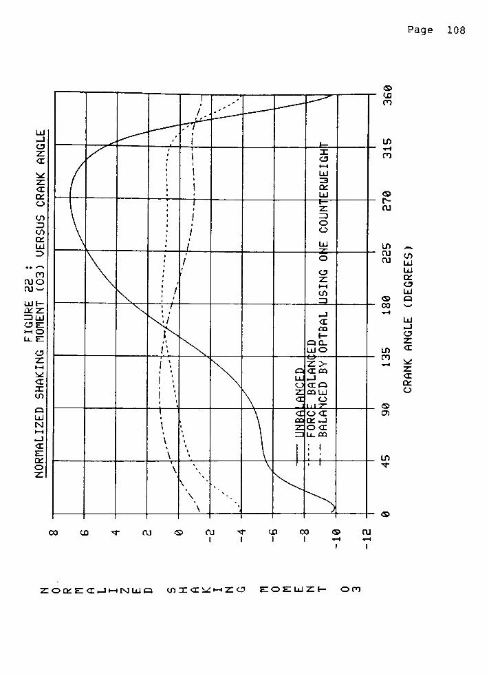
Page 108
o
z
<r
or
o
to
3
to
or
ui
o
ro
ruonjw
LUH-
orz
3LU
OZ
HO
o
z4
OI
XCO
Q
LU
Ni
<r
z
oro
*
1f
' < *
1
f
f/ X
ot 1
UI
3or
UI
\ i
- ~^=
z
3
O
o
LU-r-
\/1
i
O
o
z(1
to
3
11
/
11
1
%
1
1 '
1'
1 1
1 '.1
1'
x
Q
UJ
O
z
<r
E
11
I
\1
\
i
i
%
X
\
\*
(3d
Z
Z3
oo:
or ~i
oo:
Ll. CO
; It
\
\
\
1
. 1
CO
ro
LO
ro
ru
lo *-.
ruto
LU
LU
or
oLU
Q
00 w
*H
LU_J
C3
Z
too:
CO,-1
v
z
o:or
o
<s>
en
LO
00 CO OJ OJ
I
<J-
I
to CO
I
ru*-
i
ZOttEdJHNIiJQ (jIKT^hZO ZOZl oro

Page 109
7.0 DISCUSSION OF RESULTS
The theory and development of a computer program to balance
planar four bar linkages has been presented. The theory assumes
the links to be rigid and have a finite length. As shown in the
three example problems, the OPTBAL program is capable of
partially balancing the combined effects of the shaking force,
shaking moments, bearing forces and the input torque
Efficient determination of the kinetic quantities was
accomplished using the"direct"
approach as presented by Lee and
Cheng [21]. Counterweight sizes and angular locations were
found by adapting an existing optimization program developed by
Johnson [ 18 ] .
Although the developed program provides a superior method
of balancing linkages with rigid bodies, the author feels that
the method will not always ensure smooth operation of the
mechanism. The first, and foremost problem with the method is
the assumption of rigid links. This assumption makes the
analysis insensitive to resonant frequencies. Therefore, a
situation could exist where the linkage has been balanced from a
rigid body point of view, yet it could operate at its natural
frequency. In such a case, no matter how small the predicted
kinetic quantities are, the linkage would not be likely to
operate smoothly- A second problem may arise from the
assumption of the links and the counterweights being in the same
Page 110
plane. In many practical designs this may be difficult to
achieve, and the user must make an engineering judgement based
upon the particular geometry. The program also assumes that the
brackets which connect the counterweights, have a negligible
mass in comparison to the counterweight or link. Again, the
validity of this assumption is problem dependent and can not be
judged in general. The remainder of the assumptions , however,
should closely approximate a real linkage if proper bearings are
used, and the linkage operates at a relatively high speed.
For linkages which can be accurately modeled using the
above assumptions, the method of balancing developed in this
thesis is excellent. The degree of balance which can be
achieved has been demonstrated in three example problems, whose
results are discussed below.
In part one of example one, a comparison is shown between
the two forms of numerical integration available in the program:
Gaussian quadrature and simple summation quadrature. In
analyzing the unbalanced linkage, Gaussian quadrature provided
approximately 33 % better efficiency in evaluating the rms
shaking force, shaking moment and input torque for the same
degree of accuracy. However, the simple summation method is
still used to evaluate the final results, since it is capable of
accurately predictingmaximum quantities. In order to compare
the two forms of quadrature, the number of sampling points was
varied. For this variation, both techniques were shown to
Page 111
converge to the same solutions. Thus, the optimum number of
sampling points for an accurate, but efficient analysis was
determined for each method.
With the results of the first part of example one, the
optimization program could accurately analyze a linkage.
However, a point of significance regarding the accuracy of the
analysis should be mentioned. In many optimization problems, as
discussed by Johnson [16], equations which provide approximate
results may still yield an equally optimum solution. It has
been this author's experience with the OPTBAL program that
approximate equations ( ie. with a small number of sampling
points ), produced good optimization results. But, when the
optimum number of sampling points were used, and hence an
accurate analysis was provided, the results of the optimization
were even better. Therefore, the remaining example problems
used the optimum number of sampling points in their analyses.
In part two of example one, the effects of varying the
relative weighting factors, W^ and W2 ,on the optimization
results were shown. The investigation produced two distinctive
sets of results. First, with emphasis on both of the terms of
the objective function (ie. W =W=0.5), or with emphasis
specifically placed on the ground bearings force term (W =1,
W =0) the results of the optimization were not significantly
different. In both situations the shaking force and input
torque were reduced by approximately the same amount. That is,
Page 112
the shaking force was reduced by 87 %, and the input torque was
reduced by 89 % over the unbalanced case. The second
distinctive set of results occurred for the situation where
emphasis was only placed on the input torque term (ie. W.=0,
Wz=l). In that case the normalized input torque was reduced by
97 % , while the normalized shaking force was only reduced by
17% over the unbalanced case. From the percent reductions in
the two cases, it is obvious that the flexibility of the
objective function is limited to optimizing the combined
effects, or just balancing the input torque. This lack of
control could be due to the two terms of the objective function
not being completely independent of each other. Lee and Cheng
obtained similar results in the analysis of a different linkage.
The only valuable conclusion from both of these investigations,
is that the best overall balancing situation occurs with the
weighting factors equal to each other.
Part three of example one showed the effects of varying the
torque regional constraint on the optimization results. As can
be seen from the results, significant changes occurred only when
the maximum allowable torque was set lower than the torque for a
normal optimization (ie. where the regional constraints are
relaxed). In such cases, the regional constraint could be used
to lower the input torque an additional 7 % over the normal
optimization . But beyond that point, large regional constraint
violations occured, which indicate that a case of incompatible
specifications had been encountered. Interestingly, the amount
Page 113
of additional reduction of the torque through regional
constraint variations is approximately the same as that obtained
by modifying the objective function.
In example two, the inline linkage of example one was
balanced. Versatility of the balancing program was shown as the
number of counterweights were varied. The optimization enabled
all important dynamic reactions to be reduced from 75 % to 91 %
over the unbalanced linkage. By comparison, the method of
complete force balancing summarized by Berkoff [5] , was shown
to eliminate the shaking force, with all other kinetic
quantities increasing from 36 % to 99 %. For the case where
both the shaking force and moment are eliminated the situation
is even worse, as the remaining kinetic parameters are increased
from 51 % to 293 %. Therefore, it appears that the total
elimination of balancing quantities, such as the shaking force,
has an adverse effect on the remainder of the unbalanced
quantities, such as the bearing forces.
In example three, a four bar linkage with an offline
coupler link was balanced. The percent reductions over the
unbalanced linkage are comparable to those of example 2. For
the case of adding only one counterweight to the crank, all the
kinetic parameters are reduced by at least 84 % over the
unbalanced linkage. By contrast, the force balanced linkage
eliminated the shaking force, and decreased the remaining
balancing terms a minimum of 53 %. So, although the linkage
Page 114
balanced by the OPTBAL program produced better overall results,
the force balanced linkage did decrease all the kinetic
parameters. Therefore, the method of completely force balancing
a linkage does not always adversely effect the remaining
balancing quantities, and seems to be problem dependent. Also
evident from the results is the effect of adding additional
counterweights to the linkage. For this particular example, the
degree of balance for two and three added counterweights, was
not significantly better than placing one counterweight on the
crank. This implies that the most practical design would only
use one counterweight attached to the crank.
The balancing results of example 3 were also presented
graphically using plots of all the kinetic parameters versus the
crank angle. As can be seen in those plots, the major
differences between the balanced and unbalanced linkages, occur
at a crank angle of approximately zero. This point is where the
follower link reverses motion and its effect is reflected
throughout the linkage. The degree of balance for this example
can be measured by how well this fluctuation has been reduced.
As with the evaluation of rms quantities, the OPTBAL program was
significantly better at reducing the maximums of all the kinetic
quantities than the method of complete force balancing.
Page 115
8.0 CONCLUSIONS
1. A general computer program to partially balance the
combined effects of the shaking force, shaking moments,
bearing forces and input torque of a planar, rigid body )four
bar linkage has been successfully developed.
2. The key assumption of the entire analysis is that the
links are rigid. Therefore, the OPTBAL balancing program is
not capable of avoiding natural frequencies where the amount
of vibration would be significant.
3. The direct method of Lee and Cheng [21] provides an
efficient method for the kinetic analysis without the need for
matrix solutions. The direct approach combines the theories
of Euler and Lagrange to provide a closed form solution to
the kinetic equations.
4. The general optimization program developed by Johnson [18]
is capable of solving complicated optimization problems, such
as balancing linkages. The basic search process of the
program couples a generalized conjugate gradient search
direction technique with a univariate line search.
5. The assembled OPTBAL program as a whole, is versatile and
useful in evaluatingdifferent balancing situations. As shown
in the example problems, the number of counterweights,
regional constraint parameters, type and degree of numerical
quadrature could easily be changed.

Page 116
6. Gaussian quadrature provides the most efficient means of
numerical quadrature in the evaluation of the objective
function and other dynamic rms quantities.
7. The objective function proposed by Lee and Cheng [21],
gives a relatively good reflection of the true dynamic forces
and couples in the linkage. However, variation of the
weighting factors shows the objective function is not as
flexible as it was first proposed since, minimization of
individual parameters, such as the input torque, were only
partially successful. Before any definite conclusions can be
drawn on this point, a more thorough investigation is needed.
8. Proper choice of the torque regional constraint permitted
minimization with emphasis on that parameter. Unfortunately,
this caused some of the remaining reactions, such as the
shaking force, to be reduced less than could occur without
that regional constraint. The degree to which the input
torque could be reduced with regional constraints is
approximately the same as that obtained by varying the
objective function.
9. The method of balancing high speed linkages using the
OPTBAL program appears to be significantly better at reducing
the combined effects of imbalance, than other closed form
solution techniques, such as the method of complete force
balancing.
Page 117
9.0 RECOMMENDATIONS
1. A real linkage should be constructed and experimentally
analyzed to verify the assumptions and results of this thesis.
2. An elastic body analysis should be performed on several
linkages to determine when the rigid body assumption is valid.
References [2], [41] and [42] show techniques for analyzing four
bar linkages with nonrigid members.
3. The basic techniques of the method presented in this thesis
should be extended to balance slider cranks, six bars and other
practical linkages.
4. The computer program developed in this thesis could be made
more effective by addingpre-
and post-processors. Conceivably,
the input data could be read in interactively, while the results
could be plotted.
5. A more indepth investigation is needed to compare the OPTBAL
program to other balancing techniques that concentrate on
eliminating the combined imbalance effects, such as references
[9], [33] and [40].
6. The OPTBAL computer program should be revised so that the
kinematic equations are flexible enough to handle the general
case. For a given set of four links, there are two possible
configurations and , therefore,two possible kinematic solutions.
Currently, the program is set up to provide one of these
solutions with no flexibility to incorporate the other.
Page 118
10.0 REFERENCES
1. Bagci, C., "Complete Shaking Force and Shaking Moment
Balancing of Link Mechanisms using Balancing Idler
Loops", ASME Technical Paper No. 80-DET-100.
2. Bagci, C. , "Methods of Elastodynamics of Mechanical,Structural, and Industrial Robotic Systems", ASME
Technical Paper No. 83-WA/DSC-7.
3. Balasubramanian, S., and, Bagci, C, "Design Equations for
the Complete Force Balancing of 6R 6-Bar, and 6-Bar
Slider Crank Mechanisms", Journal of Mechanism and
Machine Theory, Vol. 13, No. 6, 1978, PP 659-674.
4. Berkoff, R.S., and Lowen, G.G., "A New Method of
Completely Force Balancing Simple Linkages", Trans.
ASME, Journal of Engineering for Industry, Vol. 91b, No.
1, Feb. 1969, PP 21-26.
5. Berkoff, R.S., "Complete Force and Moment Balancing of
Inline Four-Bar Linkages", Journal of Mechanism and
Machine Theory, Vol. 8,No. 3, 1973, pp. 397-410.
6. Berkoff, R.S., "Force Balancing of a Six-Bar Linkage",Proceedings of the 5th World Congress on Theory of
Machines and Mechanisms, 1979, pp. 1082-1085.
7. Berkoff, R.S.,"The Input Torque in Linkages", Mechanisms
and Machine Theory, Vol. 14, 1979, pp. 61-73.
8. Burden, L., Faires, J.D., and Reynolds, A.C., Numerical
Analysis, Second Edition, Prindle, Weber, and Schmidt
Publishing Co., Boston Mass., 1981, 598 pp.
9. Conte, F.L., George, G.R., Mayne, R.M. , and Sadler, J.P.,
"Optimum Mechanism Design Combining Kinematic and Dynamic
ForceConsiderations"
,Journal of Engineering for
Industry ,Vol. 97, No. 2, May 1975, pp. 662-670.
10. Dearstyne, L.G. ,"Interactive Computing Applied to the
Force Balancing of Stephenson I and II type Six-Bar
Linkages", Proceedings of the 8th Applied Mechanisms
Conference, Oklahoma State Univ. 1983, pp. 40.1-40.7 .
11. Elliot, J.L., and Tesar, D.,"The Theory of Torque, Shaking
Force, and Shaking Moment Balancing of Four Link
Mechanisms", Trans. ASME, Journal of Engineering for
Industry, Vol. 99, No. 3, Aug. 1977, pp. 715 -722.
12. Halbleib, W. ,Rochester Institute of Technology,
Rochester, NY, Private Communication.

Page 119
13. Hildebrand, F. , Introduction to Numerical Analysis,
McGraw -
Hill, New York, 1974, Second Edition.
14. Hockey, B.A.,"The Minimization of the Fluctuations in the
Input Shaft Torque in Plane Mechanisms", Mechanism and
Machine Theory, Vol. 7, 1972, pp. 335-346.
15. Janucik, F.X. , "Development and Applications of a Quadratic
Isoparametric Finite Element for Axisymmetric Stress and
Deflection Analysis", Masters Thesis, Rochester Institute
of Technology, Rochester, NY, 1974.
16. Johnson, R.C., MECHANICAL DESIGN SYNTHESIS-Creat ive Design
and Optimization, Second Edition, R. E. Krieger
Publishing Co., Melbourne, Florida, 1978, 448 pp.
17. Johnson, R.C., Opt imum Design of Mechanical Elements,Second Edition, Wiley, New York, 1980.
18. Johnson, R.C. ,"
An Extension of a Method of Optimal Design
to Systems of Mechanical Elements Having Interelated
Boudary Effects", Ph.D. Dissertation, University of
Rochester; University Microfilms International, Ann
Arbor, Michigan, 1982, Chapter 3 and Appendix A.
19. Langrana, N.A. , and Lee, T.W. , "Analysis of Dynamic Systems
using Heuristic Optimization", Trans. ASME, Journal of
Dynamical Systems Measurement and Control, Vo 1 . 1 0 2 , No .
1, March 1980, pp. 35-40.
20. Lee, T.W. , and Freudenstein, F. , "Heuristic Combinatorial
Optimization in the Kinematic Design of Mechanisms", Tans
ASME, Journal of Engineering for Industry, Vol.98, No. 4,Nov. 1976, pp. 1277-1284.
21.
22. Lowen, G.G. , and Berkoff, R S., "Survey of Investigations
into the Balancing of Linkages", Journal of Mechanisms,
Vol. 3, No. 4, 1968, pp. 221-396.
23. Lowen, G.G., and Berkoff, R.S. , "Determination of Force
Balanced Four-Bar Linkages with Optimum Shaking MomentCharacteristics"
,Trans. ASME, Journal of Engineering for
Industry, Vol. 93, No. 1, Feb. 1971, pp. 39-46.
24. Lowen, G.G., Trepper, F.R., and Berkoff, R.S.,"The
Quantitative Influence of Complete Force Balancing of
Certain Families of Four-BarLinkages"
,Mechanism and
Machine Theory, Vol. 9, 1974, pp. 299-323.

Page 120
25. Mabie, H.H., and Ocvirk, F.W., Mechanisms and Dynamics of
Machinery, Third Edition, Wiley, 1975, 594 pp.
26. Marshall, W.E., and Waldron, P., "Inertia Torques in
Four-Bar Mechanisms", Journal of Mechanical EngineeringScience, Vol. 9, No. 4, 1967, pp. 309-317.
27. Martin, G.H., Kinematics and Dynamics of Machinery. Second
Edition, McGraw-Hill, 1982, 492 pp.
28. Meirovitch, L., Methods of Analytical Dynamics,
McGraw-Hill, 1970, 524 pp.
29. Meriam, J.L., Dynamics, S.I. Version, Second Edition,
Wiley, 1975, 478 pp.
30. Oldham, K. Interactive Computing Applied to Linkage
Balancing", Computer Aided Design, Vol. 7, No. 3, July1975, pp. 142-144.
31. Oldham, K. , and Walker, M.J., "A Procedure for Force
Balancing Planar Linkages using Counterweights", Journal
of Mechanical Engineering Science , Vo 1 . 20, No . 4 ,
1978, pp. 177-182.
32. Regklaitus, G.V., Ravindran, A., and Ragsdell, K.M. ,
Engineering Optimization-Methods and Applications, Wiley,
1983, 684 pp.
33. Sadler, J. P. , "Balancing of Six-Bar Linkages by Nonlinear
Programming", Proceedings of the 4th World Congress on
Theory of Machines and Mechanisms, Sept. 1975, pp.
139-144.
34. Shigley, J.E., and Uicker, J.J., Theory of Machines and
Mechanisms, McGraw-Hill, 1980, 577 pp.
35. Smith, M.R., and Maunder, L., "Inertia Forces in a Four-Bar
Linkage", Journal of Mechanical Engineering Science, Vol.
9, No. 3, 1967, pp. 218-225.
36. Smith, M.R. , "Dynamic Analysis and Balancing of Linkages
with Interactive ComputerGraphics"
, Computer Aided
Design, Vol. 7, No. 1, July 1975, pp. 15-19.
37. Trepper, F.R., and Lowen, G.G. ,"General Theorms Concerning
Full Force Balancing of Planar Linkages by Internal Mass
Redistribution", Trans. ASME, Journal of Engineering for
Industry, Vol. 94b, No. 3, Aug. 1972, pp. 789-796.
38. Trepper, F.R., and Lowen, G.G. , "Shaking Force Optimization
of Four-Bar Linkage with Adjustable Constraints on Ground
Bearing Forces", Trans. ASME, Journal of Engineering for
Industry, Vol. 97, No. 2, May 1975, pp. 643-651.
Page 121
39. Tricamo, S.J., and Lowen, G.G.,"A Novel Method for
Prescribing the Maximum Shaking Force of a Four Bar
Linkage with Flexibility in Counterweight Design", Trans.
ASME, Journal of Mechanisms, Transmissions, and
Automation in Design, Vol. 105, No. 3, Sept. 1983, pp.
511-519.
40. Tricamo, S.J., and Lowen, G.G. , "Simultaneous Optimization
of Dynamic Reactions of a Four-Bar Linkage with
Prescribed Maximum Shaking Force", Trans. ASME, Journal
of Mechanisms Transmissions, and Automation in Design,
Vol. 105, No. 3, Sept. 1983, pp. 520-525.
41. Turcic, D.A., and Midha, A., "Dynamic Analysis of Elastic
Mechanism Systems Part I : Generalized Equations of
Motion", ASME Technical Paper No. 83-WA/DSC-43.
42. Turcic, D.A., Midha A., and Bosnik, J. R. , "Dynamic Analysis
of Elastic Mechanism Systems Part II : Applications and
Experimental Results", ASME Technical Paper No.
83-WA/DSC-38.
43. Wiederrich, J.L., and Roth, B., "Momentum Balancing of
Four-Bar Linkages", Trans. ASME, Journal of Engineeringfor Industry, Vol. 98, No. 4, Nov. 1976, pp.
1289-1295.
Page A-l
APPENDIX A
11.0 PRINCIPLES OF ANGULAR MOMENTUM
Justification of the equations used for Euler's second
law of motion are discussed below. First, a general
derivation of Euler's second law about a fixed joint will be
presented. Next, definitions of angular momentum for
different types of relative and absolute motion will be
shown. Finally, the general case of applying Euler's second
law to a two point mass model link rotating a moving point
will be given.
Consider the system of n point masses shown in Figure
Al. Each of the n particles is rigidly connected together
by internal forces, fij, and a general external load, f i i,is
applied to each. The masses have a combined center of
gravity location, C, and can be expressed in terms of either
the XYZ fixed coordinate system, or the xyz body coordinate
system. The position, velocity and acceleration of the
general point"
0"
are assumed to be known. Absolute
position of point 0 is given by r'
,and the relative
position of point C with respect to point 0 is given by r
OC

11.0 PRINCIPLES OF ANGULAR MOMENTUM Page A-2
Figure Al General System of n Point Masses Rigidly
Fixed Together
^SYSTEM
^-.^ BOUNDARY
The time derivative of the absolute angular momentum
vector for the ith particle of the system of n masses, with
respect to the fixed point0'
may be given as :
A,
= r,
O I 0 I
x m r
o ,
(Al)
where,
r,
is the absolute position vector of the ith mass.
m ' is the mass of the ith particle.
r . is the absolute acceleration vector of the ith point
-o/
mass.
Separating the ith mass from the system, Euler's second law

11.0 PRINCIPLES OF ANGULAR MOMENTUM Page A-3
of motion can be applied to a single particle.
r ,. x F.
= A , (A2)"O / ~Ri ""/
where,
F is the resultant force vector on the ith point mass
~K|
due to both externaK f- ) and internal (f:;) forces.i j 1 1
Thus, we can write equations similar to the above expression
for each of the n point masses, nij, i = 1,2
,3,
. . . ,i , . . . ,n .
Or,
r,xf +r,xf +r,xf +...+ rxf +...+ r,xf = A . (A3)~ot ~n -o, ~n -ot -is -of -//
-0'
-in -0l
r.xf +r,xf + r , x f + . . .+ r , x f +
. . .+ r
,x f = A , ( A4 )
-oz -zi-o2 ~zz -o2 -2-, -oz "zi -o^ -zn ""*
r , x f + r ' x f + r , x f +...+r,xf.+...+r,xf = A ' (A5)
-o^ -3/ ~o "32 -o3 -33 -o3 -zi -o -3n "i
r/x f. + r /x f + r,x f. +...+ r,x f.
. + ...+ r .x f - = A , (A6)
-Oi -li ~Oj -11 -os -ii "Oj -j.1 -oy -JO-Oy
r xf + r xf + r,x f +. .
.+ r xf + - +< x = A . (A7)
-o'n "hi ~on ~t)Z ~on -03 -on -ni o nn -on
To find the time derivative of the angular momentum for the system
of n particles, equations Al through A7 must be summed, or :
T i * x f-
= 7 ^'.in
'1=
(A8)

11.0 PRINCIPLES OF ANGULAR MOMENTUM Page A-4
Where the internal force cross product terms conveniently
cancel. Now, the cross product of the absolute position
vector, r'
, and the external force vector applied to the
ith mass actually form a couple about point0'
.
fa 0i Jl
Combining equations A8 and A9, the time derivative of the absolute
angular momentum can be expressed in terms of the couple about point 0.!
(A9)
C ,=
> A , (A10)
Equation A10 is the most common form of Euler's second
law, and can be used to relate couples and angular momentum
about a fixed point 0'. However, there are many different
variations of the law which stem from different definitions
of the angular momentum . The author currently knows of six
definitions for angular momentum, and these are listed in
table Al.
For the derivation of Euler's second law for a two
point mass model link which rotates about a moving point 0,
the definition given by case 4 will be used. From table Al,
the definition of angular momentum for case 4 is given as :
h
A = V r .xm. r . (All)
-oREL t_--oi 1 oi

11.0 PRINCIPLES OF ANGULAR MOMENTUM Page A-5
Taking a time derivative of the above equation produces :
*
A
-OREL(r xm.r +r xm-r )
i-l - i-0; "0; -O;(A12)
Table # Al ; Definitions of Angular Momentum
Case # Nomenclature Type of motion
Absolute Relative
1Ao'
) '.KM; f '.L* oi '-Oi
-
2 Ao'rel.-
3 Ao X f.xm-r i
*-, -o;-o,-
- *
-
4 Ao ^L-
0
5 Ac
0
-
6 Ac R.L-
0
Where the first term can be eliminated since the cross
product of two parallel vectors,is a null vector. The
relative position and acceleration vectors of the second
term can be written in terms of absolute quantities .

11.0 PRINCIPLES OF ANGULAR MOMENTUM Page A- 6
=r
,
-
r (A13)
'OT -o; -o'0
Therefore,
-o;
=
-ro;-
'
-Vo(A14)
Substituting equation A15 into A12 ,
-^rfl
=
L c o. xmi '.
"
i ' )] (A16)OREL - o; o/ oo
or,
h
A = \ [r x m, r .
-
r x m- r / ] (A17)-oKEl *- ~o; i -o- ~o;
>-oo
i ;i
Where, the resultant couple about point 0, is just the first
term in equation A17.
n
C =
) r x mr r, (A18)
Substituting A17, into equation A18, and solving for C,
-OR
n
C = A + ) f r xmr] (A19)-OR "oftfl f- "0,'
"Oohi
Equation A19 is the result we desire to apply Euler's second
law of motion to link 2 which rotates about a non-fixed

11.0 PRINCIPLES OF ANGULAR MOMENTUM Page A-7
joint. Note that for the case where the moving joint
coincides with the fixed joint (ie. r , is null), equation
-oo
A19 reduces to the form of applying the law to a fixed
joint, equation A10. Equation A19 also is the same result
as obtained by Meriam (reference [29], page 191, equation
100) .
At this point"n"
is usually allowed to go to infinity in
equations A10 and A19, so that the expression may be applied
to a real body. However, for the application of the two
point mass model we simply let n equal 2. Summarizing , the
two forms of Euler's second law applied to the two point
mass model are given by:
C/ => r >. x m r'
-OR A-f -O' ' -lon ,.,
(A20)
C = > [ r.
xm-r +r x m-r , ] (A21)
OR *rf{~ '~t ~o; '"Oo
Where equation A20 can be applied to links which rotate
about a frame joint ( eg. links 1 and 3 ), and equation A21
can be applied to links which rotate about a general moving
joint ( eg. link 2) .
Page B-l
APPENDIX B
12.0 SOLUTION OF THE TWO POINT MASS MODEL CONVERSION
The purpose of this section is to show the solution of
four equations for the conversion from a real model to a two
point mass model. As given in section 4.2, the four
equations are :
m;,+
m\i=
m\T (B1)
m; 1;,=
m;T l;r cos(0;r-
/ ) (B2)
m',zliz=
m;rl;rsin(e;T- ,' ) (B3)
z z T t
,', ln+ mizlit
=
llr+nlirm
The four unknowns of the above set equations are the
parameters of the two point mass model : mj, , mjz , l'fl ,
l'i2. Solving equation B3 for m,'z ,
m;Ti;-sin( 9 it-
J
m"
'*1
'
1\Z
Solving equation Bl for m*. ,
,',
=
miT~
miz
(B4)
(B5)
m (B6)

12.0 SOLUTION OF THE TWO POINT MASS MODEL CONVERSIONPage B-2
Substituting B5 into the above equation allows m /, to be
expressed solely in terms of 1^, and other known
quantities.
m',
=
m;T [ l,t-
l;T sin( Q;T-
9,')] (B7)
ln
Solving equation B2 for 1,', ,
lj,=
miTli'Tcos(e/r-
e; ) (B8)
mu
or, using the expression formf in equation B7,
1'
becomes,
ij,=
1/2 i/rcos(-e;r-
e;) (B9)
i;z- l;rsin(6/7- -
/)
Now, substitution of equations B5, B7 and B9 into
equation B4 will eliminate all the unknown parameters except
for1,V
2.
[ xaifil'^- i;rsin(e;T-
e; ) ][l;zlrcos(9,'T- Q; ) ] +
If2.[lij.-l;Tsin(e,V-
0;)]
*T *
+ [m;Ti;Tsin(9,y -9/) ] ljt } = I ;r+
m}r1rT (B10)
To simplify the above expression, let :
!,Vr= 1
,'t cos(e/T-
0; ) (bid
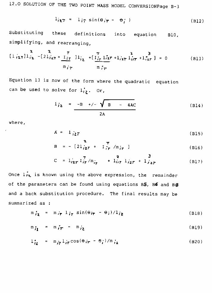
12.0 SOLUTION OF THE TWO POINT MASS MODEL CONVERSIONPage B-3
1i\t =
i;r sin(/r-
e; ) (B12)
Substituting these definitions into equation BIO,
simplifying, and rearranging,
* * T T i 3
[i.zt]i,\ -[2i,,T+_iiI ]iiz +[i;rigT+i;lTi;/T + i;ar ] = 0 (B13)
m//> m
m
Equation 13 is now of the form where the quadratic equation
can be used to solve for 1,',. Or,
1iz=
"B +/- VB - 4AC (B14)
2A
where,
A = l izT (B15)
r
XT
8 = "
[21/Er +
I;r /m;r ] (B16)
T * 3
c =
1izrlir/m1'T+ 1>'T lizr + 1
/V (B17>
Once l/i. is known using the above expression, the remainder
of the parameters can be found using equations BS, B6 and B8
and a back substitution procedure. The final results may be
summarized as :
mfi=
m>'r lir sin(eiT"
Q!^liz (B18)
m/*l=
m'V_
m/'j (B19)
1U=
m/rl;rcos(e/r-
e/l/m^ (B20)
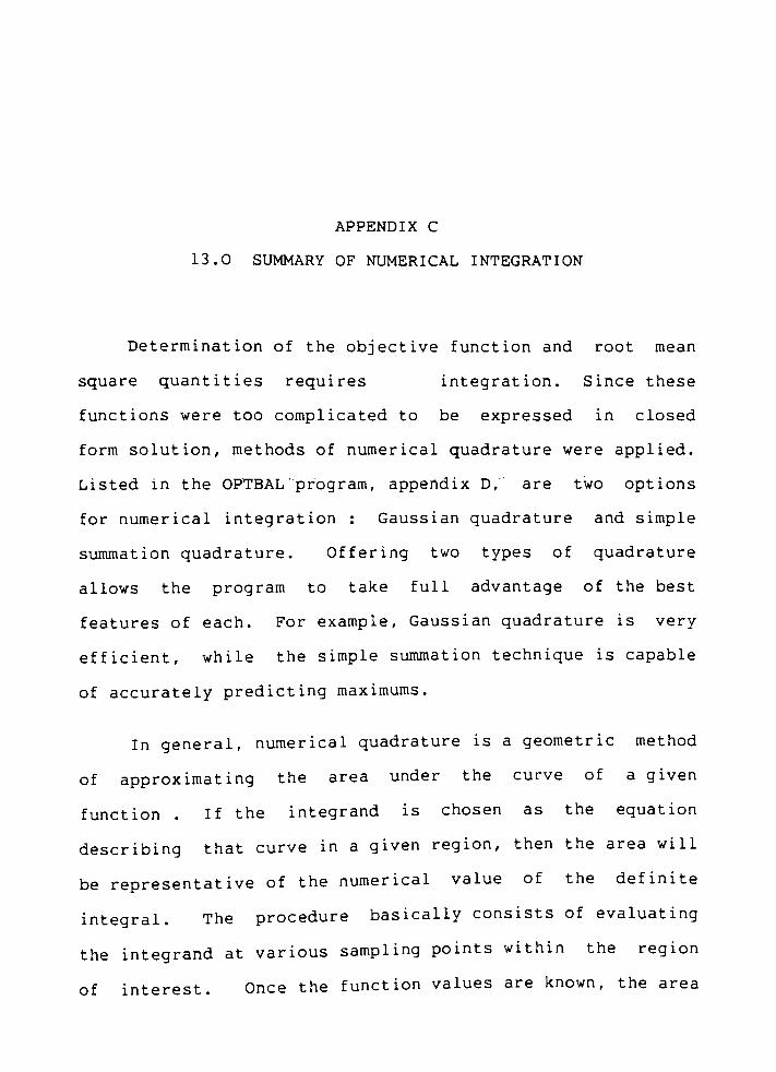
APPENDIX C
13.0 SUMMARY OF NUMERICAL INTEGRATION
Determination of the objective function and root mean
square quantities requires integration. Since these
functions were too complicated to be expressed in closed
form solution, methods of numerical quadrature were applied.
Listed in the OPTBAL program, appendix D, are two options
for numerical integration : Gaussian quadrature and simple
summation quadrature. Offering two types of quadrature
allows the program to take full advantage of the best
features of each. For example, Gaussian quadrature is very
efficient, while the simple summation technique is capable
of accurately predicting maximums.
In general, numerical quadrature is a geometric method
of approximating the area under the curve of a given
function . If the integrand is chosen as the equation
describing that curve in a given region, then the area will
be representative of the numerical value of the definite
integral. The procedure basically consists of evaluating
the integrand at various sampling points within the region
of interest. Once the function values are known, the area
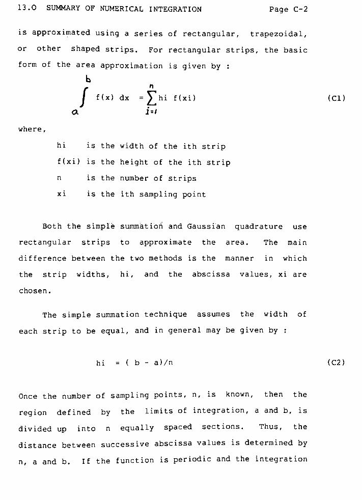
13.0 SUMMARY OF NUMERICAL INTEGRATION Page C-2
is approximated using a series of rectangular, trapezoidal,
or other shaped strips. For rectangular strips, the basic
form of the area approximation is given by :
b
/ f(x) dx =hi f(xi) (CI)
where,
a i=/
hi is the width of the ith strip
f(xi) is the height of the ith strip
n is the number of strips
xi is the ith sampling point
Both the simple summation and Gaussian quadrature use
rectangular strips to approximate the area. The main
difference between the two methods is the manner in which
the strip widths, hi, and the abscissa values, xi are
chosen.
The simple summation technique assumes the width of
each strip to be equal, and in general may be given by :
hi = ( b -
a)/n (C2)
Once the number of sampling points, n, is known, then the
region defined by the limits of integration, a and b, is
divided up into n equally spaced sections. Thus, the
distance between successive abscissa values is determined by
n, a and b. If the function is periodic and the integration
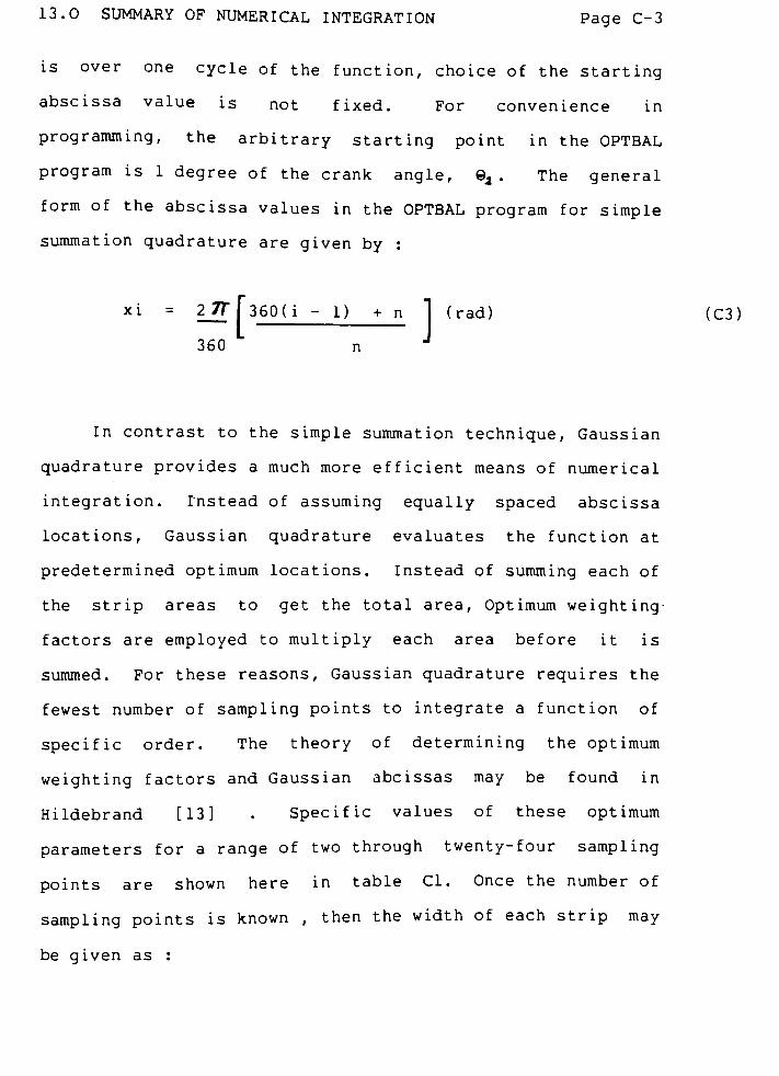
13.0 SUMMARY OF NUMERICAL INTEGRATION Page C-3
is over one cycle of the function, choice of the starting
abscissa value is not fixed. For convenience in
programming, the arbitrary starting point in the OPTBAL
program is 1 degree of the crank angle, 0a . The general
form of the abscissa values in the OPTBAL program for simple
summation quadrature are given by :
:i = 27r["360(i -
1) + n 1 (r-ad) (C3)
360"
n
In contrast to the simple summation technique, Gaussian
quadrature provides a much more efficient means of numerical
integration. Instead of assuming equally spaced abscissa
locations, Gaussian quadrature evaluates the function at
predetermined optimum locations. Instead of summing each of
the strip areas to get the total area, Optimum weighting
factors are employed to multiply each area before it is
summed. For these reasons, Gaussian quadrature requires the
fewest number of sampling points to integrate a function of
specific order. The theory of determining the optimum
weighting factors and Gaussian abcissas may be found in
Hildebrand [13] .Specific values of these optimum
parameters for a range of two through twenty-four sampling
points are shown here in table CI. Once the number of
sampling points is known ,then the width of each strip may
be given as :
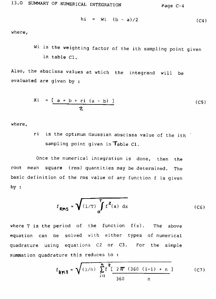
13.0 SUMMARY OF NUMERICAL INTEGRATION Page C-4
hi = Wi (b -
a)/2 (C4)
where,
Wi is the weighting factor of the ith sampling point given
in table CI.
Also, the abscissa values at which the integrand will be
evaluated are given by :
Xi = [ a + b + ri (a -
b) ]
a
where,
ri is the optimum Gaussian abscissa value of the ith"
sampling point given in Table CI.
Once the numerical integration is done, then the
root mean square (rms) quantities may be determined. The
basic definition of the rms value of any function f is given
by :
= Y (1/T) Jf2(x) dx
(C5)
fRf\S=
V (1/T) / f (x> dx (C6)
where T is the period of the function f(x). The above
equation can be solved with either types of numerical
quadrature using equations C2 or C3. For the simple
summation quadrature this reduces to :
fRf\s= V(1/n) ff2[ 27r (36 (i-1} + n 1 <C7)
360 n
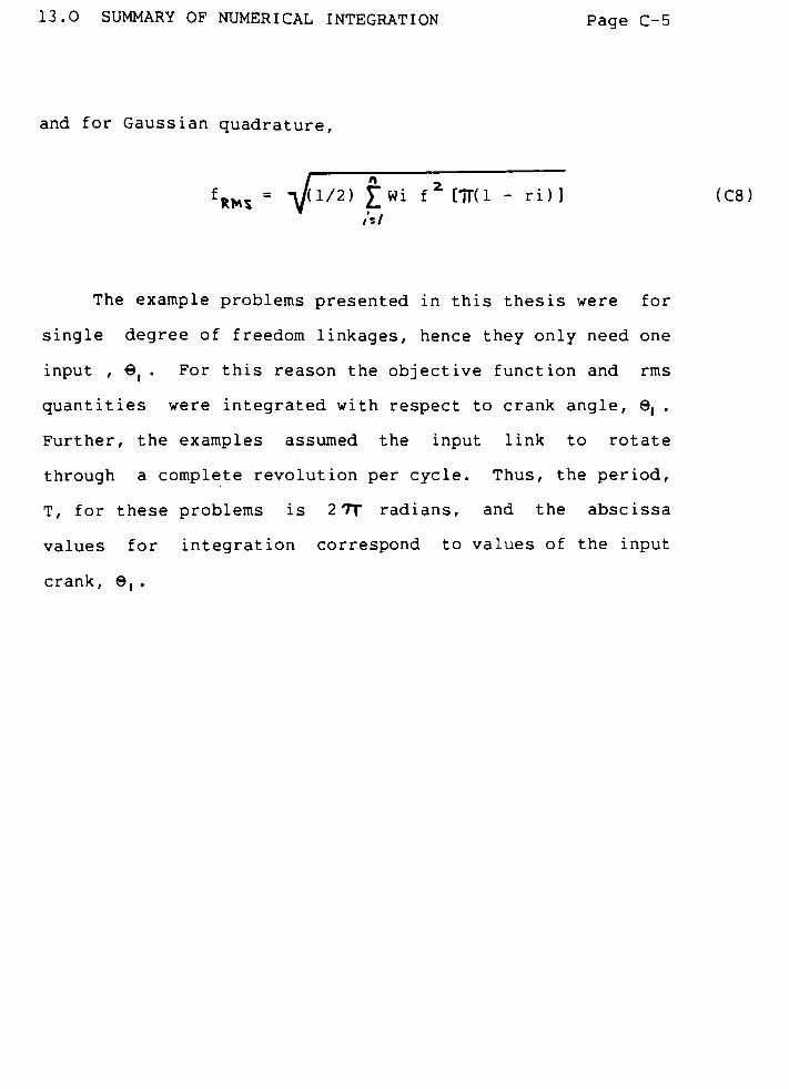
13.0 SUMMARY OF NUMERICAL INTEGRATION Page C-5
and for Gaussian quadrature,
fRMS= Y1/2) ^Wi fZ
mi ~
ri)1 (C8)
The example problems presented in this thesis were for
single degree of freedom linkages, hence they only need one
input , 0( . For this reason the objective function and rms
quantities were integrated with respect to crank angle, 9, .
Further, the examples assumed the input link to rotate
through a complete revolution per cycle. Thus, the period,
T, for these problems is 2TT radians, and the abscissa
values for integration correspond to values of the input
crank, 9, .

Page c 6
TABLE C1
ABSCISSAS AMD WEIGHT FACTORS FO GAl/SSUN INTEGRATION
Abscissas -Ai-, (Zeros of Lejvndre Polynomials) Weight Factors***,
tri
.-2
0.57735 02691 39626
0.00000 OOOOO OOQOO0.77459 46692 4148}
0.33993 10435 84354
0.86113 63115 9-1353
3.00000 00000 09090
B. 5 3 8*6 93101 05683
0.90417 9845.9 33464
0.23361 '?ISSO 8J197
0.66120 93364 66265
0.93246 95142 0J152
0.00000 ooooo ooooo
0.40584 51513 77397
0.741S3 11855 9?194
0.94913 79123 42759
1.OOOOO 00000 00000
i-3
0.33=83 33SS3 '3859
0.S3555 5555-5 55556
-4
0.6521* 5159 42546
0.34785 48451 37454
0.54353 33PS3 E3339
0.47362 6734 39346
0.236'2 i8S50 5418?
.-6
0.467OJ 37345 72631
0.34074 15730 48139
0.17132 44923 79170
-7
0.41795 nan 73469
0.38183 00505 05119
0.27970 53914 89277
0.12948 496ol 68870
*?(
0.13343 46424 95650
0.5255) 24099 16)29
0.79644 44774 13627
0.96C28 98564 97536
0.00030 00000 00033
0.32425 :42)4 03339
0.613)7 14327 00590
9.&34W 1137) 25636
0.96816 02395 07626
0.14E37 4)339 316310.-3339 53?<1 29247
0.47940 95632 9024
0.85504 3)446 8899S
0.97390 65235 17172
0.12523 34085 U469
0.36783 14939 98130
0.58731 79542 e4617
0.76990 26741 94305
0.90411 7256) 704750.98156 06342 46719
"i
.-8
-9
3.34263 373)3 73342
3.31)73 44458 77337
0.22233 10344 53374
3.13122 85362 90374
0.3332) 93550 012500.31734 70770 40CO)0.2tCM 06964 029)53.13C64 31606 94357
0.C8127 43333 61574
10
0.293=2 42247 1475)0.2=926 67193 09994
0.21908 9)625 15932
0.14945 13491 505ei
0.06667 13443 08688
12
0.24914 70453 1J40)0.23)49 25365 383550.20316 74267 230660.16007 83285 43346
0.10693 93259 953180.04717 5336) 86512
*i -16
0.09<0l 25098 376)7 440195
0.28160 35:37 792S3 91)230
0.453C1 47776 57227 335342
0.61737 62444 024JJ 743447
0.75540 44023 55003 0)3995
0.36563 12C23 973)1 743683
0.94457 30230 73232 574C79
O.98940 0"3<9 91649 932596
0.07652 45211 3)497 333755
0.22773 53511 416-5 073033
0.37370 60337 15419 56067)
0.510561 70019 50J27 09-3C04
0.6)955 36307 <.o515 02545)
0.745)3 19064 60133 797:614
0.3)U 69713 22213 32)395
0.91223 44292 51325 905563
0.96397 19272 77913 791258
0.99312 85991 BS094 924736
0.06405 63928 52405 624035
0.1=7111 93674 7)416 3C9159
0.31504 26796 96la) )74)37
0.4>)79 35075 250? 133437
0.54542 14713 e93)9 5)5d'j8
0.64309 36519 }<-975 5692'.2
0.74012 41915 73554 364244
0.82000 19E59 7)902 921954
0.38641 55270 04401 0342' 3
0.93877 45520 027)2 758^24
0.97472 95559 71309 493199
20
-Z4
0.18945 06104 55043 196235
3.13260 34150 44923 53=367
0.16915 45".9) 95002 533189
0.14959 5*353 16574 732031
0.12442 89712 55533 872052
0.09515 85llo 32492 734510
0.04225 35239 33647 397S43
0.02715 24594 11754 394652
0.15275 3)871 30725 350493
3.14917 29644 7240) 746733
0.142C9 41C93 16332 05i)29
0.13148 96)84 49176 4:&a980.11419 isjio 5i;i3 417)12
0.10193 Oll'S 17Z40 4;037
0.08327 47415 747C4 7497^50.04267 23493 )4109 '34)570
0.24040 14293 00334 941))1
0.01761 40071 39152 113)12
0.1779) 3195) 6752 15*974
0.1253) 74543 46E73 296121
0.12147 04729 2^303 331204
0.11053 54430 5)725 6J13S)
0.1C744 42701 15965 43476)
C. 39761 36521 0411) 396270
0.38619 01615 )195) 275al7
0.973)4 64314 lirei )057N
3.05329 35-*9 154)6 730744
0.:4427 74)33 17*19 334169
0.0295) 13334 2493) i.43181
0.01234 12297 99987 1995470.99518 72199 97021 360130
Compiled from P. Davis and P. Rabirw-itr Abscissas and weights for Gauvian quadratures ot high
order. J. Research NBS 56, 35-37, 1956, RP2W5; P. Davis and P. Rabinowit;. Additional abscissas
and weights fcr Gaussian quadratures of high order. Values for - -64, .SO. and%. .J. Research N'BS 69.
613-*14, 1St3. P.P2875; and .'i. N*. Lownn, N". David.-s ami A. I*cven.y?n. T.-.hlc of ;h- zeros of the Legendre
polynomials of order 1-16 and ;he might coeft.cii-uls .'or
Gauss'
mechanical quadrature "formula. Bull.
Amer. Math. Soc. 4*8. 7C9-743, 1942 iwnh pt-rrnissioii).
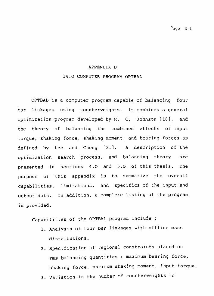
Page D-l
APPENDIX D
14.0 COMPUTER PROGRAM OPTBAL
OPTBAL is a computer program capable of balancing four
bar linkages using counterweights. It combines a general
optimization program developed by R. C. Johnson [18], and
the theory of balancing the combined effects of input
torque, shaking force, shaking moment, and bearing forces as
defined by Lee and Cheng [21]. A description of the
optimization search process, and balancing theory are
presented in sections 4.0 and 5.0 of this thesis. The
purpose of this appendix is to summarize the overall
capabilities, limitations, and specifics of the input and
output data. In addition, a complete listing of the program
is provided.
Capabilities of the OPTBAL program include :
1. Analysis of four bar linkages with offline mass
distributions .
2. Specification of regional constraints placed on
rms balancing quantities : maximum bearing force,
shaking force, maximum shaking moment, input torque,
3. Variation in the number of counterweights to
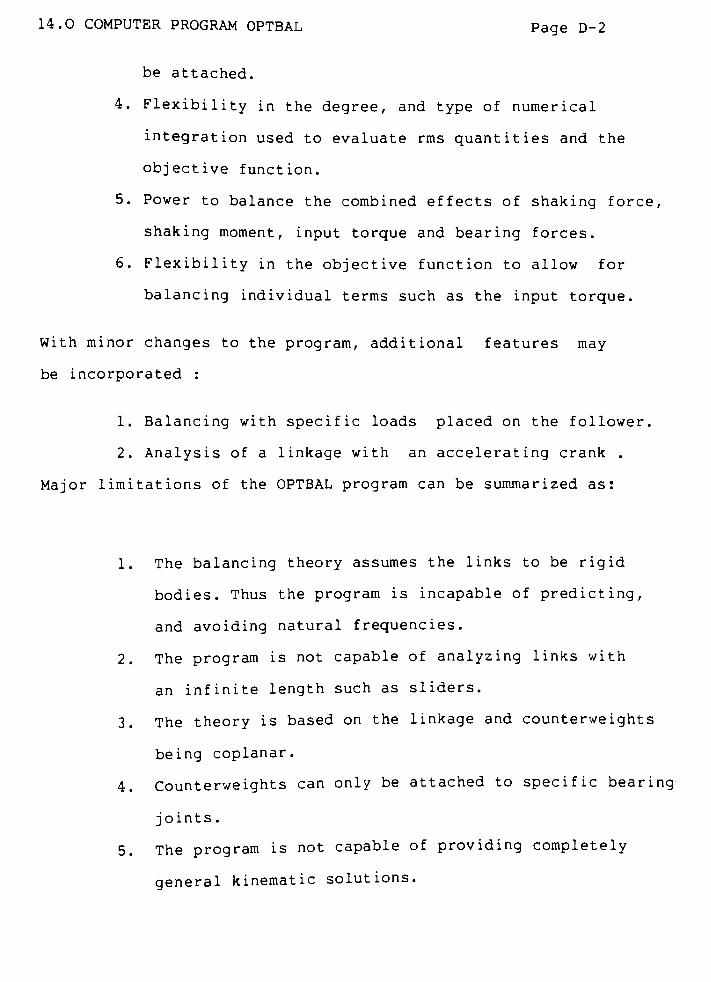
14.0 COMPUTER PROGRAM OPTBAL Page D-2
be attached.
4. Flexibility in the degree, and type of numerical
integration used to evaluate rms quantities and the
objective function.
5. Power to balance the combined effects of shaking force,
shaking moment, input torque and bearing forces.
6. Flexibility in the objective function to allow for
balancing individual terms such as the input torque.
With minor changes to the program, additional features may
be incorporated :
1. Balancing with specific loads placed on the follower.
2. Analysis of a linkage with an accelerating crank .
Major limitations of the OPTBAL program can be summarized as:
1. The balancing theory assumes the links to be rigid
bodies. Thus the program is incapable of predicting,
and avoiding natural frequencies.
2. The program is not capable of analyzing links with
an infinite length such as sliders.
3. The theory is based on the linkage and counterweights
being coplanar.
4. Counterweights can only be attached to specific bearing
joints .
5. The program is not capable of providing completely
general kinematic solutions.
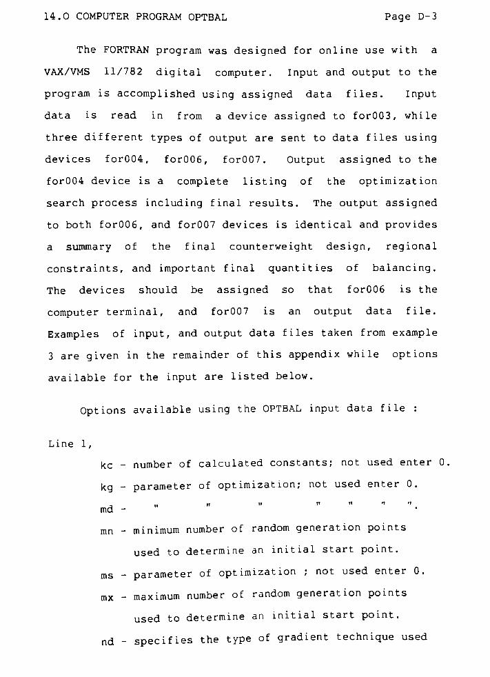
14.0 COMPUTER PROGRAM OPTBAL Page D-3
The FORTRAN program was designed for online use with a
VAX/VMS 11/782 digital computer. Input and output to the
program is accomplished using assigned data files. Input
data is read in from a device assigned to for003, while
three different types of output are sent to data files using
devices for004, for006, for007. Output assigned to the
for004 device is a complete listing of the optimization
search process including final results. The output assigned
to both for006, and for007 devices is identical and provides
a summary of the final counterweight design, regional
constraints, and important final quantities of balancing.
The devices should be assigned so that for006 is the
computer terminal, and for007 is an output data file.
Examples of input, and output data files taken from example
3 are given in the remainder of this appendix while options
available for the input are listed below.
Options available using the OPTBAL input data file :
Line 1,
kc - number of calculated constants; not used enter 0
kg- parameter of optimization; not used enter 0.
md-
mn- minimum number of random generation points
used to determine an initial start point.
ms- parameter of optimization ; not used enter 0.
mx- maximum number of random generation points
used to determine an initial start point.
nd- specifies the type of gradient technique used
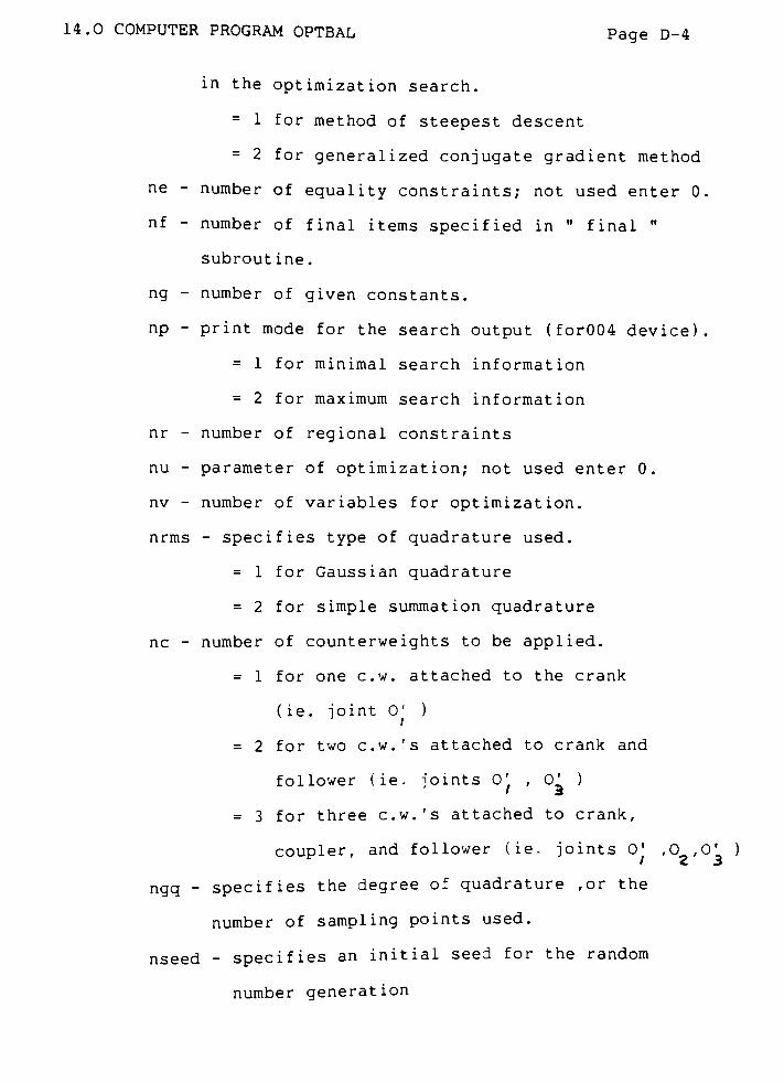
14.0 COMPUTER PROGRAM OPTBAL Page D-4
in the optimization search.
= 1 for method of steepest descent
= 2 for generalized conjugate gradient method
ne-
number of equality constraints; not used enter 0-
nf-
number of final items specified in"
final"
subroutine.
ng-
number of given constants.
np-
print mode for the search output (for004 device).
= 1 for minimal search information
= 2 for maximum search information
nr-
number of regional constraints
nu-
parameter of optimization; not used enter 0.
nv-
number of variables for optimization.
nrms-
specifies type of quadrature used.
= 1 for Gaussian quadrature
= 2 for simple summation quadrature
nc-
number of counterweights to be applied.
= 1 for one c.w. attached to the crank
( ie. joint0'
)
= 2 for two c.w.'s attached to crank and
follower (ie. joints 0^ ,
0'
)
= 3 for three c.w.'s attached to crank,
coupler, and follower (ie. joints0'
ngq- specifies the degree of quadrature ,or the
number of sampling points used.
nseed- specifies an initial seed for the random
number generation
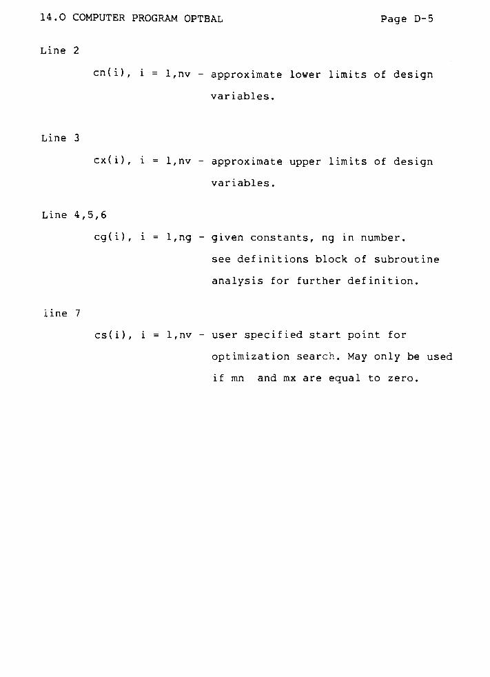
14.0 COMPUTER PROGRAM OPTBAL Page D-5
Line 2
cn(i), i = l,nv -
approximate lower limits of design
variables.
Line 3
cx(i), i = l,nv -
approximate upper limits of design
variables.
Line 4,5,6
cg(i), i = l,ng-
given constants, ng in number.
see definitions block of subroutine
analysis for further definition.
line 7
cs(i), i = 1,nv
-
user specified start point for
optimization search. May only be used
if mn and mx are equal to zero.
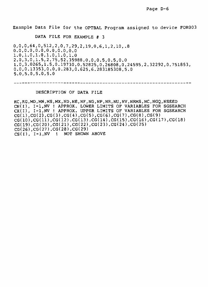
Page D-6
Example Data File for the OPTBAL Program assigned to device FOR003
DATA FILE FOR EXAMPLE # 3
0,0,0,64,0,512,2,0,7,29,2,19,0,6,1,2,10, .80.0,0.0,0.0,0.0,0.0,0.0
1.0,1.0,1.0,1.0,1.0,1.0
2.0,3.0,1.5,2.75,52.35988,0.0,0.5,0.5,0.0
1.0,3.0265,1.5,0.19730,0.52825,0.26808,0.24595,2.32292,0.751853,
0.0,0.13353,0.0,0.283,0.625,6.28318 5308,5.0
5.0,5.0,5.0,5.0
DESCRIPTION OF DATA FILE
KC , KG ,MD
,MN ,MS ,
MX,ND
, NE ,NF
, NG ,NP
,NR
, NU ,NV
,NRMS , NC , NGQ ,
NSEED
CN(I), I=1,NV ! APPROX. LOWER LIMITS OF VARIABLES FOR SGSEARCH
CX(I), I=1,NV ! APPROX. UPPER LIMITS OF VARIABLES FOR SGSEARCH
CG(1),CG(2),CG(3) ,CG(4),CG(5),CG(6),CG(7),CG(8) ,CG(9)
CG(10),CG(11) ,CG(12) ,CG(13),CG(14),CG(15),CG(16),CG(17) ,CG(18)
CG(19),CG(20),CG(21) ,CG( 22 ) ,CG( 23 ) ,CG< 24 ) ,CG(25)
CG(26),CG(27) ,CG(28) ,CG(29)
CS(I), I=1,NV ! NOT SHOWN ABOVE
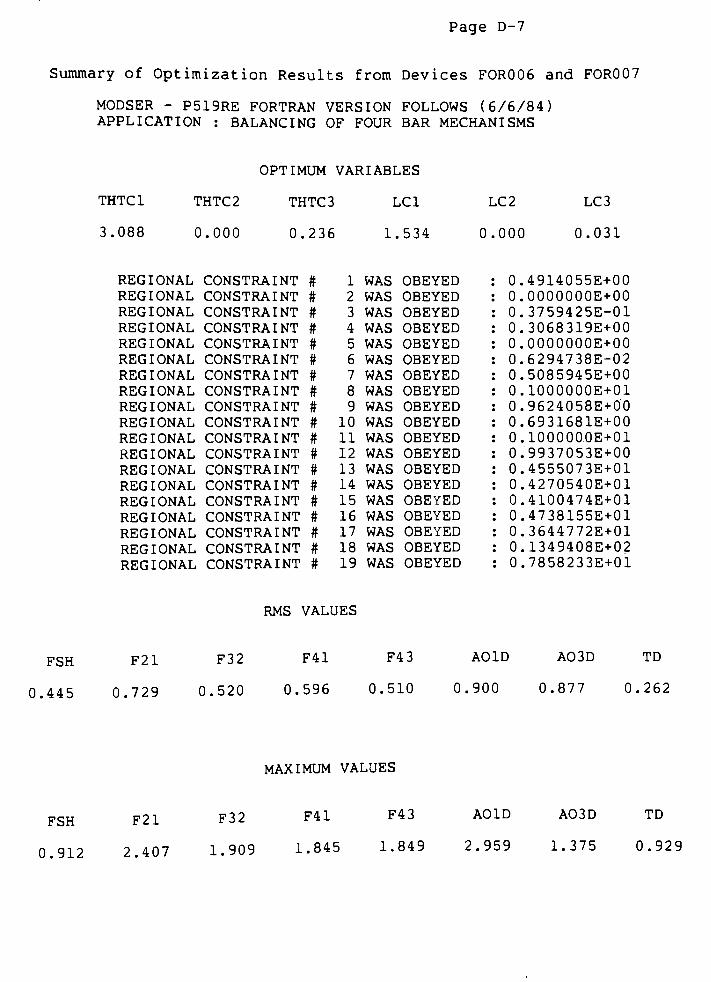
Page D-7
Summary of Optimization Results from Devices FOR006 and FOR007
MODSER -
P519RE FORTRAN VERSION FOLLOWS (6/6/84)APPLICATION : BALANCING OF FOUR BAR MECHANISMS
OPTIMUM VARIABLES
THTC1 THTC2 THTC3 LCI LC2 LC3
3.088 0.000 0.236 1. 534 0.000 0.031
REGIONAL CONSTRAINT # 1 WAS OBEYED : 0. 4914055E+00
REGIONAL CONSTRAINT # 2 WAS OBEYED 0. 0000000E+00
REGIONAL CONSTRAINT # 3 WAS OBEYED 0. 3759425E-01
REGIONAL CONSTRAINT # 4 WAS OBEYED 0. 3068319E+00
REGIONAL CONSTRAINT # 5 WAS OBEYED 0. 0000000E+00
REGIONAL CONSTRAINT # 6 WAS OBEYED 0. 6294738E-02
REGIONAL CONSTRAINT # 7 WAS OBEYED 0. 5085945E+00
REGIONAL CONSTRAINT # 8 WAS OBEYED 0. 1000000E+01
REGIONAL CONSTRAINT # 9 WAS OBEYED 0 9624058E+00
REGIONAL CONSTRAINT # 10 WAS OBEYED 0 6931681E+00
REGIONAL CONSTRAINT # 11 WAS OBEYED . 0 1000000E+01
REGIONAL CONSTRAINT # 12 WAS OBEYED 0 9937053E+00
REGIONAL CONSTRAINT # 13 WAS OBEYED : 0 4555073E+01
REGIONAL CONSTRAINT # 14 WAS OBEYED : 0 .4270540E+01
REGIONAL CONSTRAINT # 15 WAS OBEYED : 0 .4100474E+01
REGIONAL CONSTRAINT # 16 WAS OBEYED : 0 .4738155E+01
REGIONAL CONSTRAINT # 17 WAS OBEYED : 0 .3644772E+01
REGIONAL CONSTRAINT # 18 WAS OBEYED : 0 .1349408E+02
REGIONAL CONSTRAINT # 19 WAS OBEYED : 0 .7858233E+01
RMS VALUES
FSH F21 F32 F41 F43 AOID A03D TD
0.445 0.729 0.520 0.596 0.510 0. 90 D 0.877 0.262
MAXIMUM VALUES
FSH
0.912
F21
2.407
F32
1.909
F41
1.845
F43
1.849
AOID
2.959
A03D
1.375
TD
0.929
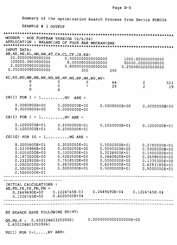
Page D-8
Summary of the optimization Search Process from Device FOR004
EXAMPLE # 3 OUTPUT
MODSER - AOD FORTRAN VERSION (6/6/84)APPLICATION : BALANCING OF FOUR BAR MECHANISMS
******************************************************INPUT DATA:
AB,AE,AG,AL,AM,AW,AT,CA,CL,CF,JX,KX=
10.00000000000000 0.5000000000000000 1000.000000000000100000.0000000000 8.000000000000000 20000.000000000002.000000000000000 0.8500000000000000 0.25000000000000000.2500000000000000 300 250
KC,KG,MD,MN,MS,MX,ND,NE,NF,NG,NP,NR,NU,NV=
0 0 0 64 0 5122 0 7 29 2 190 6
CN(I) FOR I = 1, ,NV ARE =
0.0000000E+00 0.0000000E+00 0.0000000E+00 0.0000000E+000.0000000E+00 0.0000000E+00
0.1000000E+01
0.1000000E+01
0.1000000E+01
0.1000000E+01
0.1000000E+01 0.1000000E+01
CG(IG) FOR IG = 1, . . . ,NG ARE =
0.2000000E+01
0.5235988E+02
0.0000000E+00
0.1973000E+00
0.2322920E+01
0.0000000E+00
0.5000000E+01
0.5000000E+01
0.3000000E+01
0.0000000E+00
0.1000000E+01
0.5282500E+00
0.7518530E+00
0.2830000E+00
0.5000000E+01
0.1500000E+01
0.5000000E+00
0.3026500E+01
0.2680800E+00
O.OOOOOOOE+00
0.6250000E+00
0.5000000E+01
0.2750000E+01
0.5000000E+00
0.1500000E+01
0.2459500E+00
0.1335300E+0O
0.6283185E+01
0.5000000E+01
0.2449490E-04 0,
INITIAL CALCULATIONS
AD,FD,FS,FX,FH,FM =
0.2449490E+00 0
0.1224745E+00 0
.1224745E-03
.4000000E+04
.1224745E-04
SG SEARCH GAVE FOLLOWING POINT:
QG,PG,X : 0.4322246032509261 0 . 0000000000000000E+00
0.4322246032509261
VG(I) FOR 1=1, . . . ,NVARE=
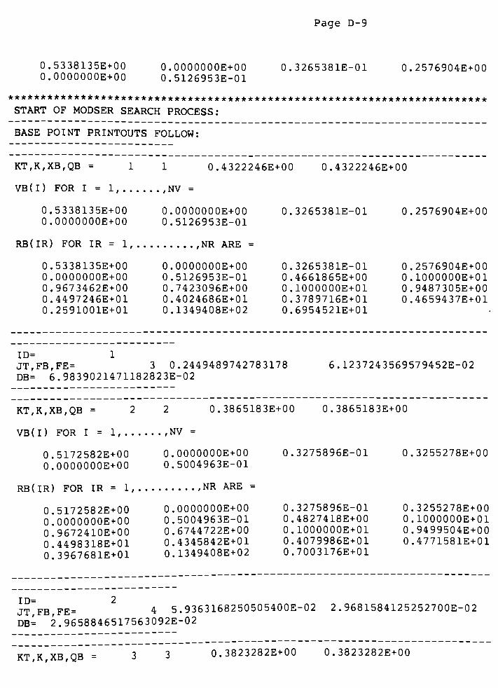
Page D-9
0.5338135E+00 O.OOOOOOOE+00 0 . 3265381E-01 0 . 2576904E+00
O.OOOOOOOE+00 0.5126953E-01
***********************************************
START OF MODSER SEARCH PROCESS:
BASE POINT PRINTOUTS FOLLOW:
KT,K,XB,QB=11 0.4322246E+00 0 . 4322246E+00
VB ( I ) FOR I = 1, , NV =
0.5338135E+00 0 . 0000000E+00 0 . 3265381E-01 0 . 2576904E+00
O.OOOOOOOE+00 0.5126953E-01
RB(IR) FOR IR = 1, ,NR ARE =
0.5338135E+00 O.OOOOOOOE+00 0 . 3265381E-01 0 . 2576904E+00
O.OOOOOOOE+00 0.5126953E-01 0 . 4661865E+00 0 . 1000000E+01
0.9673462E+00 0 . 7423096E+00 0 . 1000000E+01 0 . 9487305E+00
0.4497246E+01 0 . 4024686E+01 0 . 3789716E+01 0 . 4659437E+01
0.2591001E+01 0.1349408E+02 0 . 6954521E+01
ID= 1
JT,FB,FE= 3 0.2449489742783178 6 . 1237243569579452E-02
DB= 6.9839021471182823E-02
KT,K,XB,QB=22 0 . 3865183E+00 0 . 3865183E+00
VB(I) FOR I = 1, ,NV
=
0.5172582E+00 0 . 0000000E+00 0 . 3275896E-01 0 . 3255278E+00
o!oOOOOOOE+00 0.5004963E-01
RB(IR) FOR IR = 1, ,NR ARE =
0 5172582E+00 0 .0000000E+00 0 . 3275896E-01 0 . 3255278E+00
0'0000000E+00 0.5004963E-01 0 . 4827418E+00 0 . 1000000E+01
0*9672410E+00 0 .6744722E+00 0 . 1000000E+01 0 . 9499504E+00
0*4498318E+01 0 .4345842E + 01 0 . 4079986E + 01 0 . 4771581E + 01
0*3967681E+01 0 .1349408E+02 0 . 7003 176E+01
ID= 2
JT FB FE= 4 5.9363168250505400E-02 2 . 9681584125252700E-02
DB= 2.9658846517563092E-02
KT K XB QB = 3 3 0 .3823282E+00 0 . 3823282E+00

Page D-10
VB(I) FOR I = 1, fNV=
0.4879059E+00
0.0000000E+00O.OOOOOOOE+00
0.4810785E-01
RB(IR) FOR IR = 1, ,NR ARE =
0.4879059E+00
O.OOOOOOOE+00
0.9670026E+00
0.4527117E+01
0.3960623E+01
O.OOOOOOOE+00
0.4810785E-01
0.6782483E+00
0.4332337E+01
0.1349408E+02
0.3299738E-01
0.3299738E-01
0.5120941E+00
0.1000000E+01
0.4022520E+01
0.7078063E+01
0.3217517E+00
0.3217517E+00
0.1000000E+01
0.9518921E+00
0.4766868E+01
ID= 2JT,FB,FE= 2 2.5210019539928628E-02 2 . 5210019539928628E-02DB= 1.3894205963529090E-02
KT,K,XB,QB=44 0 . 3805351E+00 0 . 3805351E+00
VB(I) FOR I = 1, ,NV=
0.4898797E+00
O.OOOOOOOE+00
0.0000000E+00
0.4725271E-01
RB(IR) FOR IR = 1, ,NR ARE =
0.4898797E+00 0,
0.0000000E+00 0,
0.9668881E+00 0.
0.4554355E+01 0,
0.3659149E+01 0.
0000000E+00
4725271E-01
6919745E+00
4279460E+01
1349408E+02
0.3311195E-01
0.3311195E-01
0.5101203E+00
0.1000000E+01
0.4106564E+01
0.7110007E+01
0.3080255E+00
0.3080255E+00
0.1000000E+01
0.9527473E+00
0.4748406E+01
ID= 2
JT,FB,FE= 4 1.1810075068999726E-02 5 . 9050375344998631E-03DB= 4.6777076705050751E-03
KT,K,XB,QB=55 0 . 3804845E+00 0 . 3804845E+00
VB(I) FOR I = 1, ,NV
=
0.4928252E+00
0.00000OOE+0O
O.OOOOOOOE+00
0.4364785E-01
0.3354937E-01
RB(IR) FOR IR = 1, ,NR ARE =
0.4928252E+00
0.0000000E+00
0.9664506E+00
O.OOOOOOOE+OO
0.4364785E-01
0.6918395E+00
0.3354937E-01
0.5071748E+00
0.1000000E+01
0.3081605E+00
0.3081605E+00
0.1000000E+01
0.9563522E+00
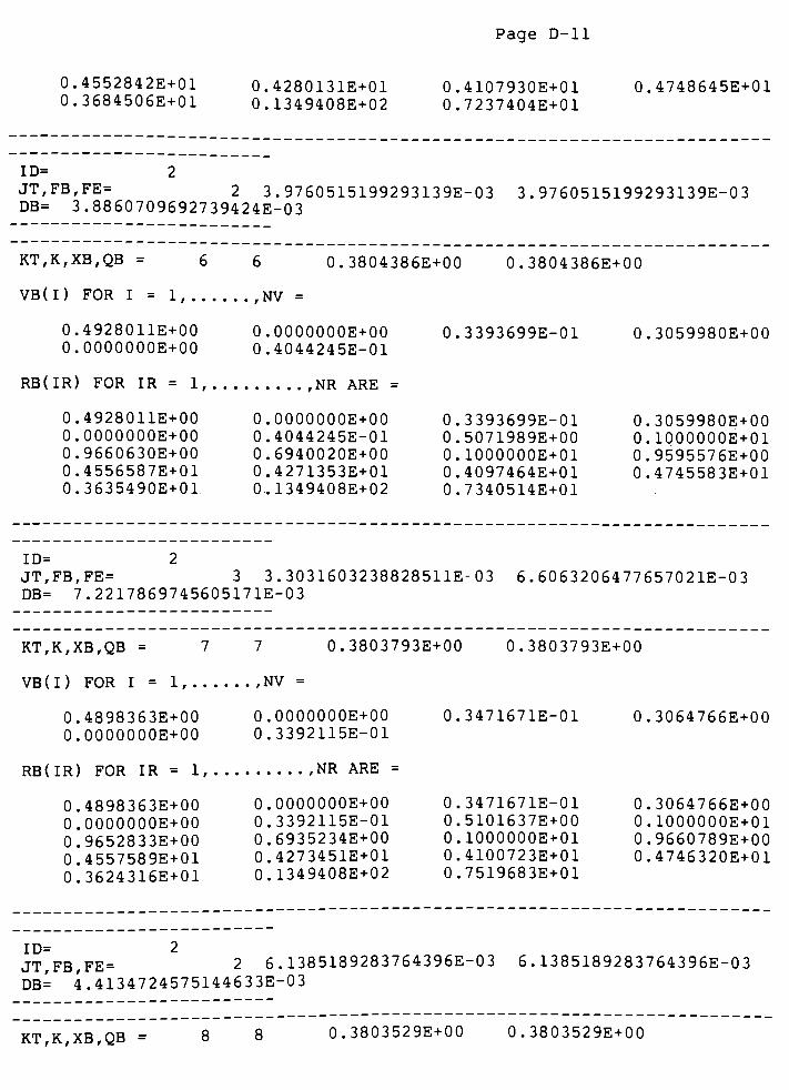
Page D-ll
0.4552842E+01
0.3684506E+010.4280131E+01
0.1349408E+02
0.4107930E+01
0.7237404E+01
0.4748645E+01
ID= 2JT,FB,FE=
2 3.9760515199293139E-03 3 . 9760515199293139E-03DB= 3.8860709692739424E-03
KT,K,XB,QB=66 0 . 3804386E+00 0 . 3804386E+00
VB(I) FOR I = 1, ,NV=
0.4928011E+00
O.OOOOOOOE+00
O.OOOOOOOE+00
0.4044245E-01
0.3393699E-01 0.3059980E+00
0,
1 JVUK IK =
1,
.4928011E+00 0,.0000000E+00
0,0000000E+00 0,.4044245E-01
0,.9660630E+00 0,.6940020E+00
0,.4556587E+01 0,.4271353E+01
0,.3635490E+01 0.,.1349408E+02
0.3393699E-01
0.5071989E+00
0.1000000E+01
0.4097464E+01
0.7340514E+01
0.3059980E+00
0.1000000E+01
0.9595576E+00
0.4745583E+01
ID= 2
JT,FB,FE= 3 3.3031603238828511E-03 6 . 6063206477657021E-03DB= 7.2217869745605171E-03
KT,K,XB,QB=77 0 . 3803793E+00 0 . 3803793E+00
VB ( I ) FOR I = 1 , ,NV =
0.4898363E+00
0.0000000E+00
RB(IR) FOR IR = 1,
0.4898363E+00
0.0000000E+00
0.9652833E+00
0.4557589E+01
0.3624316E+01
0,
0,
.0000000E+00
.3392115E-01
0..3471671E-01
. . . . ,NR ARE =
0,
0.
0,
0.
0,
0,
0,
0,
0,
0,
.0000000E+00
.3392115E-01
.6935234E+00
.4273451E+01
.1349408E+02
.3471671E-01
.5101637E+00
.1000000E+01
.4100723E+01
.7519683E+01
0.3064766E+00
0.3064766E+00
0.1000000E+01
0.9660789E+00
0.4746320E+01
ID= 2
JT,FB,FE= 2 6.1385189283764396E-03 6 . 1385189283764396E-03
DB= 4.4134724575144633E-03
KT,K,XB,QB = 0.3803529E+00 0 . 3803529E+00
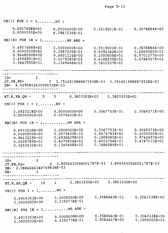
Page D-12
VB(I) FOR I = 1, ,NV=
0.4907658E+00 0
0.0000000E+00 0
0000000E+0O
2987235E-01
RB(IR) FOR IR = 1, ,NR ARE =
0.4907658E+00 0,
0.0000000E+00 0,
0.9648050E+00 0
0.4554891E+01 0
0.3663550E+01 0
0000000E+0O
2987235E-01
6921116E+00
4279280E+01
1349408E+02
0.3519501E-01
0.3519501E-01
0.5092342E+00
0.1000000E+01
0.4108239E+01
0.7610107E+01
0.3078884E+00
0.3078884E+00
0.1000000E+01
0.9701277E+00
0.4748357E+01
ID= 2
JT,FB,FE= 2 3.7514515888872938E-03 3 . 7514515888872938E-03
DB= 4.5295802430590338E-03
KT,K,XB,QB=99 0 . 3803303E+00 0 . 3803303E+00
VB ( I ) FOR I = 1, ,
NV =
0.4923218E+00
0.0000000E+00
0.0000000E+00
0.2575432E-01
RB(IR) FOR IR = 1, ,NR ARE =
0.4923218E+00 0
0.0000000E+00 0
0.9643225E+00 0
0.4555789E+01 0
0.3653532E+01 0
0000000E+0O
2575432E-01
6930629E+00
4275424E+01
1349408E+02
0.3567753E-01
0.3567753E-01
0.5076782E+00
0.1000000E+01
0.4103704E+01
0.7686085E+01
0.3069371E+00
0.3069371E+00
0.1000000E+01
0.9742457E+00
0.4747012E+01
ID= 2
JT,FB,FE= 2 3.8501432066001787E-03 3 . 8501432066001787E-03
DB= 2.0886666348769838E-03
ME= 1
KT K XB QB = 10 1 0 . 3803230E+00 0 . 3803230E+00
VB ( I ) FOR I = 1 , ,NV =
0 4915353E+00 0 .00OO000E+0O 0 . 3588663E-01 0 . 3063338E+00
O.'OOOOOOOE+OO0.2392778E-01
RB(IR) FOR IR = 1, 'NRARE =
0 4915353E+00 0 .0000000E+0O 0 . 3588663E-01 0 . 3063338E+00
0!0000000E+000.2392778E-01 0 . 5084647E+00 0 . 1000000E+01
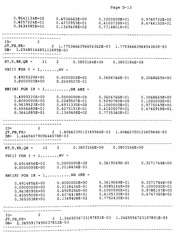
Page D-13
0.9641134E+00
0.4557224E+01
0.3634585E+01
0.6936662E+00
0.4272953E+01
0.1349408E+02
0.1000000E+01
0.4100730E+01
0.7714801E+01
0.9760722E+00
0.4746150E+01
ID= 2
JT,FB,FE= 2 1.7753666396454362E-03 1 . 7753666396454362E-03DB= 1.6548516485112899E-03
KT,K,XB,QB 11 2 0 . 3803184E+00 0 . 3803184E+00
VB ( I ) FOR I = 1, ,NV=
0.4909220E+00
O.OOOOOOOE+00
0.4909220E+00
0.0000000E+00
0.9639523E+00
0.4556680E+01
0.3641885E+01
O.OOOOOOOE+00
0.2249507E-01
RB(IR) FOR IR = 1, ,NR ARE =
0.0000000E+00
0.2249507E-01
0.6931335E+00
0.4275151E+01
0.1349408E+02
0.3604766E-01
0.3604766E-01
0.5090780E+00
0.1000000E+01
0.4103.507E+01
0.7735260E+01
0.3068665E+00
0.3068665E+00
0.1000000E+01
0.9775049E+00
0.4746918E+01.
ID= 2
JT,FB,FE= 2 1.4066239012345964E-03 1 . 4066239012345964E-03
DB= 1.4665407909644578E-03
KT,K,XB,QB 12 3 0 . 3803156E+00 0 . 3803156E+00
VB ( I ) FOR I = 1, ,
NV =
0.4914856E+00 0
0.0000000E+00 0
0.4914856E+00
O.OOOOOOOE+00
0.9638095E+00
0.4555900E+01
0.3653038E+01
OOOOOOOE+OO
2118434E-01
RB(IR) FOR IR = 1, ,NR ARE =
0. 0000000E+00
0.2118434E-01
0.6928256E+00
0.4276418E+01
0.1349408E+02
0.3619049E-01
0.3619049E-01
0.5085144E+00
0.1000000E+01
0.4105120E+01
0.7752430E+01
0.3071744E+00
0.3071744E+00
0.1000000E+01
0.9788157E+00
0.4747360E+01
ID= 2
JT,FB,FE= 2 1,
DB=1.3655917490037812E-
2465596723197891E-03
03
1.2465596723197891E-03
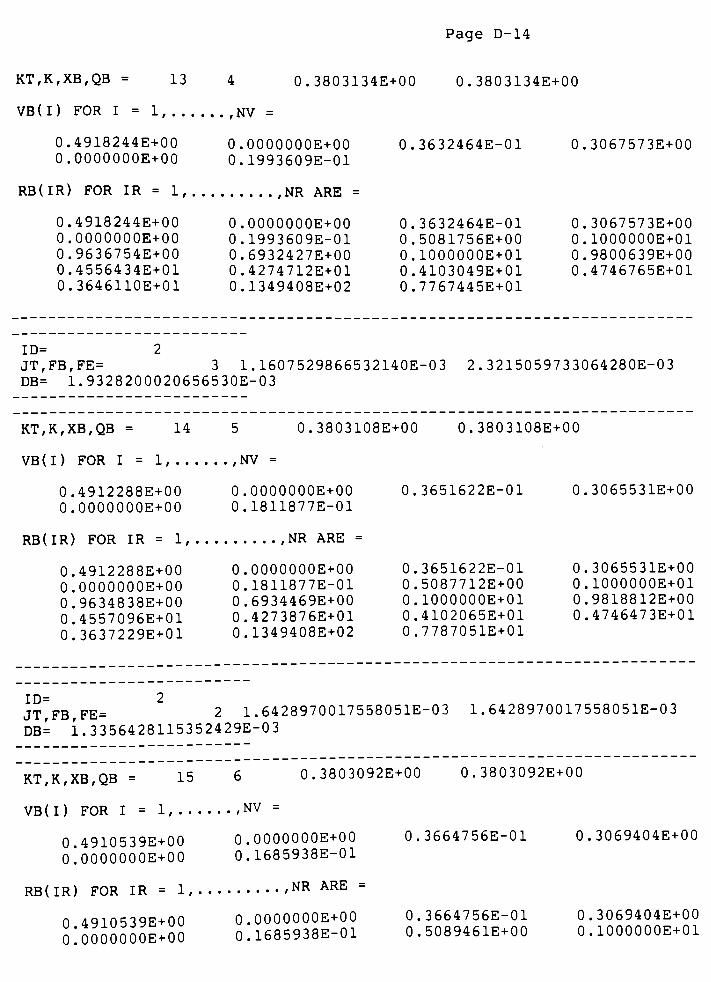
Page D-14
KT,K,XB,QB = 13
VB(I) FOR I = 1, . .
0.4918244E+00
0. 0000000E+00
0.4918244E+00
0.0000000E+00
0.9636754E+00
0.4556434E+01
0.3646110E+01
0.3803134E+00 0.3803134E+00
,NV=
0. 0000000E+00
0.1993609E-01
RB(IR) FOR IR = 1, ,NR ARE =
0. 0000000E+00
0.1993609E-01
0.6932427E+00
0.4274712E+01
0.1349408E+02
0.3632464E-01
0.3632464E-01
0.5081756E+00
0.1000000E+01
0.4103049E+01
0.7767445E+01
0.3067573E+00
0.3067573E+00
0.1000000E+01
0.9800639E+00
0.4746765E+01
ID= 2
JT,FB,FE= 3 1.1607529866532140E-03 2 . 3215059733064280E-03
DB= 1.9328200020656530E-03
KT,K,XB,QB 14 5 0 . 3803108E+00 0 . 3803108E+00
VB(I) FOR I = 1, ,NV
=
0.4912288E+00 0
O.OOOOOOOE+00 0
0000000E+00
1811877E-01
RB(IR) FOR IR = 1, ,NR ARE =
0.4912288E+00
O.OOOOOOOE+00
0.9634838E+00
0.4557096E+01
0.3637229E+01
O.OOOOOOOE+00
0.1811877E-01
0.6934469E+00
0.4273876E+01
0.1349408E+02
0.3651622E-01
0.3651622E-01
0.5087712E+00
0.1000000E+01
0.4102065E+01
0.7787051E+01
0.3065531E+00
0.3065531E+00
0.1000000E+01
0.9818812E+00
0.4746473E+01
ID= 2
JT FB FE= 2 1.6428970017558051E-03 1 . 6428970017558051E-03
DB= 1.3356428115352429E-03
~KT~K~XB~QB~= 15 6 0.3803092E+00 0 . 3803092E+00
VB ( I ) FOR I = 1, ,
NV =
0.4910539E+00 0 .0000000E+00 0 . 3664756E-01 0 . 3069404E+00
o!oOOOOOOE+000.1685938E-01
RB(IR) FOR IR = 1, 'NRARE =
n 4qin539E+00 0 .0000000E+00 0 . 3664756E-01 0 . 3069404E+00
OIOOOOOOOE+OO0.1685938E-01 0 . 5089461E+00 0 . 1000000E+01
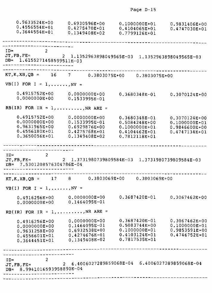
Page D-15
0.9633524E+00
0.4556554E+01
0.3644554E+01
0.6930596E+00
0.4275470E+01
0.1349408E+02
0.1000000E+01
0.4104065E+01
0.7799126E+01
0.9831406E+00
0.4747030E+01
ID= 2JT,FB,FE=
2 1.1352963898049565E-03 1 . 1352963898049565E-03DB= 1.6155271458599511E-03
KT,K,XB,QB 16 7 0.3803075E+00 0 . 3803075E+00
VB(I) FOR I = 1, ,NV=
0.4915752E+00 0
O.OOOOOOOE+00 0
0000000E+00
1533995E-01
0.3680348E-01
RB(IR) FOR IR = 1, ,NR ARE =
0.4915752E+00
O.OOOOOOOE+00
0.9631965E+00
0.4556180E+01
0.3650056E+01
O.OOOOOOOE+00
0.1533995E-01
0.6929876E+00
0.4275768E+01
0.1349408E+02
0.3680348E-01
0.5084248E+00
0.1000000E+01
0.4104462E+01
0.7812118E+01
0.3070124E+00
0.3070124E+00
0.1000000E+01
0.9846600E+00
0.4747134E+01
ID= 2
JT,FB,FE= 2 1.3731980739809584E-03 1 . 3731980739809584E-03DB= 7.5301208576304786E-04
KT,K,XB,QB 17 8 0 . 3803069E+00 0 . 3803069E + 00
VB ( I ) FOR I = 1 , ,NV =
0.4916256E+00
O.OOOOOOOE+00
RB(IR) FOR IR = 1,
0.4916256E+00
O.OOOOOOOE+00
0.9631258E+00
0.4556601E+01
0.3644451E+01
0.
0,
.0000000E+00
.1464095E-01
0..3687420E-01 0..3067462E+00
. . . . ,NR ARE =
0.
0.
0.
0,
0.
.3687420E-01
.5083744E+00
.1000000E+01
.4103124E+01
.7817535E+01
0.
0,
0.
0,
0,
0,
0,
0.
0,
.0000000E+00
.1464095E-01
.6932538E+00
.4274676E+01
.1349408E+02
.3067462E+00
,1000000E+01
.9853591E+00
.4746752E+01
ID= 2
JT,FB,FE= 26.4006027289859068E-
DB= 8.9941016593958890E-04
04 6.4006027289859068E-04
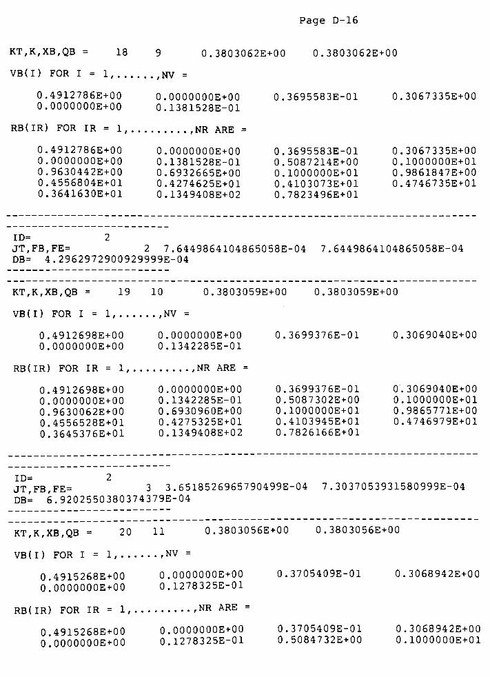
Page D-16
KT,K,XB,QB = 18
VB ( I ) FOR I = 1, . .
0.4912786E+00
0.0000000E+00
0.4912786E+00
O.OOOOOOOE+00
0.9630442E+00
0.4556804E+01
0.3641630E+01
0.3803062E+00 0.3803062E+00
,NV=
O.OOOOOOOE+00
0.1381528E-01
RB(IR) FOR IR = 1, ,NR ARE =
O.OOOOOOOE+00
0.1381528E-01
0.6932665E+00
0.4274625E+01
0.1349408E+02
0.3695583E-01
0.3695583E-01
0.5087214E+00
0.1000000E+01
0.4103073E+01
0.7823496E+01
0.3067335E+00
0.3067335E+00
0.1000000E+01
0.9861847E+00
0.4746735E+01
ID= 2
JT,FB,FE= 2 7.6449864104865058E-04 7 . 6449864104865058E-04
DB= 4.2962972900929999E-04
KT,K,XB,QB = 19 10 0 . 3803059E+00 0 . 3803059E+00
VB ( I ) FOR I = 1, ,
NV =
0.4912698E+00
0.0000000E+00
RB(IR) FOR IR = 1,
0.4912698E+00
0.0000000E+00
0.9630062E+00
0.4556528E+01
0.3645376E+01
ID= 2
JT,FB,FE= 3 3.6518526965790499E-04 7 . 3037053931580999E-04
DB= 6.9202550380374379E-04
KT,K,XB,QB = 20 11 0 . 3803056E+00 0 . 3803056E+00
VB ( I ) FOR I = 1 , ,NV =
0.4915268E+00 0 .0000000E+00 0 . 3705409E-01 0 . 3068942E+00
0!0000000E+00 0.1278325E-01
0.
0,
.0000000E+00
.1342285E-01
, , , . ,NR ARE =
0..3699376E-01 0..3069040E+00
0,
0,
0,
0,
0,
.0000000E+00
.1342285E-01
.6930960E+00
.4275325E+01
.1349408E+02
0,
0,
0,
0,
0,
.3699376E-01
.5087302E+00
.1000000E+01
.4103945E+01
.7826166E+01
0,
0,
0,
0,
.3069040E+00
.1000000E+01
.9865771E+00
.4746979E+01
RB(IR) FOR IR = 1, ,NR ARE =
0.4915268E+00
0.0000000E+00
O.OOOOOOOE+00
0.1278325E-01
0.3705409E-01
0.5084732E+00
0.3068942E+00
0.1000000E+01
Page D-17
0.9629459E+00
0.4556416E+01
0.3647053E+01
0.6931058E+00
0.4275285E+01
0.1349408E+02
0.1000000E+01
0.4103904E+01
0.7830297E+01
0.9872168E+00
0.4746965E+01
ID= 2
JT,FB,FE= 2 5.8822167823318223E-04 5 . 8822167823318223E-04DB= 4.2005326995943158E-04
KT,K,XB,QB = 21 12 0 . 3803054E+00 0 . 3803054E+00
VB ( I ) FOR I = 1, ,NV=
0.4915157E+00 0
0.0000000E+00 0
0000000E+00
1238985E-01
RB(IR) FOR IR = 1, ,NR ARE =
0.4915157E+00 0
O.OOOOOOOE+00 0
0.9629095E+00 0
0.4556660E+01 0
0.3643786E+01 0
0000000E+00
1238985E-01
6932481E+00
4274702E+01
1349408E+02
0.3709045E-01
0.3709045E-01
0.5084843E+00
0.1000000E+01
0.4103187E+01
0.7832705E+01
0.3067519E+00
0.3067519E+00
0.1000000E+01
0.9876102E+00
0.47467.61E+01
ID= 2
JT,FB,FE= 3 3.5704527946551685E-04 7 . 1409055893103370E-04
DB= 8.1021432201085169E-04
KT,K,XB,QB = 22 13 0 . 3803050E+00 0 . 3803050E+00
VB ( I ) FOR I = 1, ,
NV =
0.4912762E+00
O.OOOOOOOE+00
RB(IR) FOR IR = 1,
0.4912762E+00
0.0000000E+00
0.9628395E+00
0.4556737E+01
0.3642672E+01
0.
0.
.0000000E+00
.1161958E-01
0..3716047E-01 0..3067810E+00
, . . . ,NR ARE =
0.
0,
0,
0,
0,
.3716047E-01
.5087238E+00
.1000000E+01
.4103343E+01
.7837132E+01
0.
0,
0,
0,
0,
0,
0,
0,
0,
.0000000E+00
.1161958E-01
.6932190E+00
.4274821E+01
.1349408E+02
.3067810E+00
.1000000E+01
.9883804E+00
.4746803E+01
ID= 2
JT,FB,FE= 2 6.8868217370922394E-04
DB= 5.0593985414189779E-04
6.8868217370922394E-04
Page D-18
KT,K,XB,QB = 23
VB ( I ) FOR I = 1, . .
14 0.3803049E+00 0.3803049E+00
,NV=
0.4913114E+00
0.0000000E+00O.OOOOOOOE+00
0.1113538E-01
0.3720383E-01 0.3069166E+00
RB(IR) FOR IR = 1fNR ARE =
0.4913114E+00 0,
0.0000000E+00 0
0.9627962E+00 0
0.4556495E+01 0
0.3645971E+01 0
0000000E+00
1113538E-01
6930834E+00
4275379E+01
1349408E+02
0.3720383E-01
0.5086886E+00
0.1000000E+01
0.4104037E+01
0.7839725E+01
0.3069166E+00
0.1000000E+01
0.9888646E+00
0.4746998E+01
ID= 2
JT,FB,FE= 3 4.3004887602061313E-04 8 . 6009775204122625E-04DB= 8.2783578907076507E-04
KT,K,XB,QB = 24 15 0 . 3803046E+00 0 . 3803046E+00
VB(I) FOR I = 1, ,NV=
0.4915256E+00
0.0000000E+00
RB(IR) FOR IR = 1,
0.4915256E+00
0.0000000E+00
0.9627258E+00
0.4556474E+01
0.3646392E+01
0,
0,
.0000000E+00
.1034052E-01
. . . . ,NR ARE =
0,.3727419E-01 0,.3068650E+00
0.
0,
0,
0,
0.
.0000000E+00
.1034052E-01
.6931350E+00
.4275167E+01
.1349408E+02
0,
0,
0,
0,
0,
.3727419E-01
.5084744E+00
.1000000E+01
.4103782E+01
.7843671E+01
0,
0,
0,
0.
.3068650E+00
.1000000E+01
.9896595E+00
.4746924E+01
ID= 2
JT,FB,FE= 2 7.0366042071015032E-04 7 . 0366042071015032E-04
DB= 4.3391137284254786E-04
KT,K,XB,QB = 25 16 0 . 3803044E + 00 0 . 3803044E + 00
VB ( I ) FOR I = 1, ,
NV =
0.4914743E+00 0 .0000000E+00 0 . 3731036E-01 0 . 3067549E+00
0.0000000E+00 0.9925533E-02
RB(IR) FOR IR = 1, NR ARE =
0.4914743E+00
0.0O0O000E+00
0.0000000E+00
0.9925533E-02
0.3731036E-01
0.5085257E+00
0.3067549E+00
0.1000000E+01
Page D-19
0.9626896E+00 0 . 6932451E+00 0 . lOOOOOOE+01 0 .9900745E+00
0.4556684E+01 0 . 4274715E+01 0 . 4103227E+01 0 .4746766E+01
0.3643553E+01 0 . 1349408E+02 0 . 7845582E+01
ID= 2JT,FB,FE=
3 3.6882466691616568E-04 7 . 3764933383233136E-04DB= 5.6758356923161516E-04
KT,K,XB,QB = 26 17 0 . 3803043E+00 0 . 3803043E+00
VB(I) FOR I = 1, ,NV=
0.4913170E+00 O.OOOOOOOE+00 0 . 3735690E-01 0 . 3068089E+00
0.0000000E+00 0.9384848E-02
RB(IR) FOR IR = 1 ,NR ARE =
0.4913170E+00 0 . 0000000E+00 0 . 3735690E-01 0 . 3068089E+00
O.OOOOOOOE+00 0.9384848E-02 0 . 5086830E+00 0 . 1000000E+01
0.9626431E+00 0 . 6931911E+00 0 . 1000000E+01 0 . 9906152E+00
0.4556677E+01 0 . 4274937E+01 0 . 4103505E+01 0 . 4746844E+01
0.3643602E+01 0 . 1349408E+02 0 . 7847921E+01
ID= 2
JT,FB,FE= 2 4.8244603384687289E-04 4 . 8244603384687289E-04
DB= 2.8595332097067067E-04
KT,K,XB,QB = 27 18 0 . 3803042E+00 0 . 3803042E+00
VB ( I ) FOR I = 1 , ,NV =
0.4913655E+00 0 . 0000000E+00 0 . 3737966E-01 0 . 3068862E+00
0.0000000E+00 0.9114787E-02
RB(IR) FOR IR = 1, ,NR ARE =
0.4913655E+00 0 .0000000E+00 0 . 3737966E-01 0 . 3068862E+00
0'0000000E+00 0.9114787E-02 0 . 5086345E+00 0 . 1000000E+01
0*9626203E+00 0 .6931138E+00 0 . 1000000E+01 0 . 9908852E+00
0*4556524E+01 0 .4275254E+01 0 . 4103899E+01 0 . 4746955E+01
o!3645690E+01 0 .1349408E+02 0 . 7849027E+01
ID= 2
JT FB FE= 2 2.4306032282507008E-04 2 . 4306032282507008E-04
DB= 3.5956267187905253E-04
Page D-20
KT,K,XB,QB = 28
VB ( I ) FOR I = 1, . .
0.4914741E+00
0.0000000E+00
19 0.3803041E+00 0.3803041E+00
0.4914741E+00
0.0000000E+00
0.9625923E+00
0.4556546E+01
0.3645464E+01
,NV=
O.OOOOOOOE+00
0.8776245E-02
RB(IR) FOR IR = 1, ,NR ARE =
O.OOOOOOOE+00
0.8776245E-02
0.6931596E+00
0.4275066E+01
0.1349408E+02
0.3740772E-01 0.3068404E+00
0,.3740772E-01 0,.3068404E+00
0,.5085259E+00 0,.1000000E+01
0,.1000000E+01 0,.9912238E+00
0,.4103669E+01 0,.4746889E+01
0,.7850356E+01
ID= 2
JT,FB,FE= 2 3.0562827109719465E-04 3 . 0562827109719465E-04
DB= 2.2000370171683276E-04ME= 2
KT,K,XB,QB 29 1 0 . 3803041E+00 0 .3803041E+00
VB ( I ) FOR I = 1, ,
NV =
0.4914306E+00 0 . 0000000E+00 0 . 3742444E-01 0 . 3067825E+00
0.0000000E+00 0.8569172E-02
RB(IR) FOR IR = 1, ,NR ARE =
0.4914306E+00 0 . 0000000E+00 0 . 3742444E-01 0 . 3067825E+00
O.OOOOOOOE+OO 0.8569172E-02 0 . 5085694E+00 0 . 1000000E+01
0.9625756E+00 0 . 6932175E+00 0 . 1000000E+01 0 . 9914308E+00
0.4556664E+01 0 . 4274829E+01 0 . 4103376E+01 0 . 4746806E+01
0.3643849E+01 0 . 1349408E+02 0 . 7851138E+01
ID= 2
JT,FB,FE= 3 1.8700314645930785E-04 3 . 7400629291861570E-04
DB= 2.9832641858849662E-04
KT,K,XB,QB 30 2 0 .3803040E + 00 0 . 3803040E + 00
VB(I) FOR I = 1, ,NV
=
0.4913459E+00 0.0000000E+00 0 . 3744684E-01 0 . 3068238E+00
0!0000000E+00 0.8287015E-02
RB(IR) FOR IR = 1, ,NR ARE =
0.4913459E+00 0.0000000E+00 0 . 3744684E-01 0 . 3068238E+00
Page D-21
O.OOOOOOOE+OO
0.9625532E+00
0.4556640E+01
0.3644150E+01
0.8287015E-02
0.6931762E+00
0.4274999E+01
0.1349408E+02
0.5086541E+00
0.1000000E+01
0.4103587E+01
0.7852165E+01
0.1000000E+01
0.9917130E+00
0.4746865E+01
ID= 2JT,FB,FE= 2 2.5357745580022213E-04 2 . 5357745580022213E-04DB= 2.3954323740189937E-04
KT,K,XB,QB 31 3 0 . 3803040E+00 0 . 3803040E+00
VB(I) FOR I = 1, ,NV=
0.4913917E+00
O.OOOOOOOE+00
RB(IR) FOR IR = 1,
0.4913917E+00
0.0000000E+00
0.9625354E+00
0.4556531E+01
0.3645639E+01
O.OOOOOOOE+00
0.8058268E-02
0.3746458E-01 0.3068752E+00
0,.0000000E+00 0,.3746458E-01
0,.8058268E-02 0,.5086083E+00
0,.6931248E+00 0,.lOOOOOOE+01
0..4275210E+01 0,.4103850E+01
0,.1349408E+02 0,.7852967E+01
0.3068752E+00
0.1000000E+01
0.9919417E+00
0.4746939E+01
ID= 2
JT,FB,FE= 3 2.0361175179161447E-04 4 . 0722350358322894E-04DB= 3.2948527594401108E-04
KT,K,XB,QB 32 4 0 . 3803040E+00 0 . 3803040E+00
VB ( I ) FOR I = 1 ,NV =
0.4914680E+00
0.0000000E+00
RB(IR) FOR IR = 1,
0.4914680E+00
0.0000000E+00
0.9625112E+00
0.4556566E+01
0.3645211E+01
0,
0,
.OOOOOOOE+OO
.7741712E-02
0,.3748883E-01
, . . . ,NR ARE =
0.
0,
0.
0,
0,
0.
0,
0,
0,
0.
.0000000E+00
.7741712E-02
.6931689E+00
.4275029E+01
.1349408E+02
.3748883E-01
.5085320E+00
.1000000E+01
.4103627E+01
.7854030E+01
0.3068311E+00
0.3068311E+00
0.1000000E+01
0.9922583E+00
0.4746876E+01
ID= 2
JT,FB,FE= 2 2.8006248455240942E-04
DB= 2.9561938103743855E-04
2. 8 0062484 55240 94 2E-04
Page D-22
KT,K,XB,QB 33 5 0 . 3803039E+00 0 . 3803039E+00
VB ( I ) FOR I = 1, , nv=
0.4914148E+00 O.OOOOOOOE+00 0 . 3751034E-01 0 . 3067822E+00
0.0000000E+00 0.7455852E-02
RB(IR) FOR IR = 1, fNR ARE =
0.4914148E+00 O.OOOOOOOE+00 0 . 3751034E-01 0 . 3067822E+00
0.0000000E+00 0.7455852E-02 0 . 5085852E+00 0 . 1000000E+01
0.9624897E+00 0 . 6932178E+00 0 . 1000000E+01 0 . 9925441E+00
0.4556675E+01 0 . 4274828E+01 0 . 4103380E+01 0 . 4746806E+01
0.3643728E+01 0 . 1349408E+02 0 . 7854945E+01
ID= 2
JT,FB,FE= 2 2.5127647388182277E-04 2 . 5127647388182277E-04
DB= 3.4771213680814373E-04
KT,K,XB,QB 34 6 0 . 380 3039E+00 0 . 3803039E+00
VB(I) FOR I = *1, ,NV=
0.4913477E+00 0 . 0000000E+00 0 . 3753547E-01 0 . 3068296E+00
0.0000000E+00 0.7118901E-02
RB(IR) FOR IR = 1, ,NR ARE =
0.4913477E+00 0 . 0000000E+00 0 . 3753547E-01 0 . 3068296E+00
0.0000000E+00 0.7118901E-02 0 . 5086523E+00 0 . 1000000E+01
0.9624645E+00 0 . 6931704E+00 0 . 1000000E+01 0 . 9928811E+00
0.4556631E+01 0 . 4275023E+01 0 . 4103622E+01 0 . 4746874E+01
0.3644293E+01 0 . 1349408E+02 0 . 7855969E+01
ID= 2
JT,FB,FE= 2 2.9555531628692217E-04 2 . 9555531628692217E-04
DB= 2.9398327743749250E-04
KT,K,XB,QB = 35 7 0 .3803038E+00 0 . 3803038E+00
VB ( I ) FOR I = 1 , ,NV =
0.4914038E+00 0 .0000000E+00 0 . 3755639E-01 0 . 3068707E+00
0!0000000E+00 0.6834011E-02
RB(IR) FOR IR = 1, fNRARE =
0.4914038E+00 0 .0000000E+00 0 . 3755639E-01 0 . 3068707E+00
Page D-23
O.OOOOOOOE+OO
0.9624436E+00
0.4556535E+01
0.3645627E+01
0.6834011E-02
0.6931293E+00
0.4275191E+01
0.1349408E+02
0.5085962E+00
0.1000000E+01
0.4103832E+01
0.7856790E+01
0.1000000E+01
0.9931660E+00
0.4746933E+01
ID= 2JT,FB,FE= 2 2.4988578582186862E-04 2 . 4988578582186862E-04DB= 2.7820386460300374E-04
KT,K,XB,QB 36 8 0 . 3803038E+00 0 . 3803038E+00
VB ( I ) FOR I = 1, ,
NV =
0.4914549E+00 0,
0.0000000E+00 0.
00OO0O0E+0O
6564820E-02
0.3757596E-01 0.3068267E+00
RB(IR) FOR IR = 1, ,NR ARE =
0.4914549E+00 0
0.0000000E+00 0
0.9624240E+00 0
0.4556582E+01 0
0.3645018E+01 0
0000000E+00
6564820E-02
6931733E+00
4275011E+01
1349408E+02
0,.3757596E-01 0,. 3068267E+00
0,.5085451E+00 0,.1000000E+01
0,.1000000E+01 0..9934352E+00
0,.41036I0E+01 0,.4746870E+01
0,.7857528E+01
ID= 2
JT,FB,FE= 2 2.3647328491255318E-04 2 . 3647328491255318E-04
DB= 1.4477154122509679E-04
KT,K,XB,QB 37 9 0 . 3803038E+00 0 . 3803038E + 00
VB(I) FOR I = 1, ,NV
=
0.4914228E+00 0
0.0O0000OE+00 0
0000000E+00
6425377E-02
RB(IR) FOR IR = 1, ,NR ARE =
0.4914228E+00 0
0.0000000E+00 0
0.9624141E+00 0
0.4556631E+01 0
0.3644344E+01 0
0000000E+00
6425377E-02
6931929E+00
4274930E+01
1349408E+02
0.3758592E-01
0.3758592E-01
0.5085772E+00
0.1000000E+01
0.4103511E+01
0.7857896E+01
0.3068071E+00
0.3068071E+00
0.1000000E+01
0.9935746E+00
0.4746841E+01
ID= 2
JT,FB,FE= 2 1.2305581004133227E-04
DB= 6.5887444842649220E-05
1.2305581004133227E-04
Page D-24
KT,K,XB,QB = 38 10 0 . 3803038E+00 0 . 3803038E+00
VB ( I ) FOR I = 1, , NV =
0.4913991E+00 0 . 0000000E+00 0 . 3758987E-01 0 . 3068299E+00
0.0000000E+00 0.6368425E-02
RB(IR) FOR IR = 1, ,NR ARE =
0.4913991E+00 0.0000000E+00 0 . 3758987E-01 0 . 3068299E+00
0.0000000E+00 0.6368425E-02 0 . 5086009E+00 0 . 1000000E+01
0.9624101E+00 0 . 6931701E+00 0 . 1000000E+01 0 . 9936316E+00
0.4556605E+01 0 . 4275024E+01 0 . 4103627E+01 0 .4746874E+01
0.3644679E+01 0 . 1349408E+02 0 . 7858044E+01
ID= 2
JT,FB,FE= 2 5.6004328116251838E-05 5 . 6004328116251838E-05
DB= 2.9526784119060994E-05
KT,K,XB,QB = 39 11 0 . 3803038E+00 0 . 3803038E+00 - -
VB ( I ) FOR I = 1, ,
NV =
0.4914052E+00 0 . 0000000E+00 0 . 3759165E-01 0 . 3068334E+00
0.0000000E+00 0.6339805E-02
RB(IR) FOR IR = 1, ,NR ARE =
0.4914052E+00 0 . 0000000E+00 0 . 3759165E-01 0 . 3068334E+00
0.0000000E+00 0.6339805E-02 0 . 5085948E+00 0 . 1000000E+01
0.9624083E+00 0 . 6931666E+00 0 . 1000000E+01 0 . 9936602E+00
0.4556596E+01 0 . 4275038E+01 0 . 4103644E+01 0 . 4746879E+01
0.3644802E+01 0 .1349408E+02 0 . 7858118E+01
ID= 2
JT FB FE= 3 2.5097766501201845E-05 5 . 0195533002403690E-05
DB= 2.6306105594259598E-05
KT K XB QB = 40 12 0 .3803038E + 00 0 . 3803038E + 00
VB(I) FOR I = 1, ,NV
=
0.4914099E+00 0.0000000E+00 0 . 3759317E-01 0 . 3068284E+00
0!0000000E+00 0.6314448E-02
RB(IR) FOR IR = 1, 'NRARE =
0.4914099E+00 0 .0000000E+00 0 . 3759317E-01 0 . 3068284E+00

Page D-25
O.OOOOOOOE+00 0.6314448E-02 0 . 5085901E+00 0 .1000000E+01
0.9624068E+00 0 . 6931716E+00 0 . lOOOOOOE+01 0 . 9936856E+00
0.4556602E+01 0 . 4275018E+01 0 . 4103619E+01 0 . 4746872E+01
0.3644724E+01 0 . 1349408E+02 0 . 7858182E+01
ID= 2
JT,FB,FE= 2 2.2360189755120659E-05 2 . 2360189755120659E-05DB= 1.1450402586579092E-05ME= 3
KT,K,XB,QB 41 1 0 . 3803038E+00 0 . 3803038E+00
VB ( I ) FOR I = 1, ,NV=
0.4914085E+00 O.OOOOOOOE+00 0 . 3759382E-01 0 . 3068278E+00
0.0000000E+00 0.6303109E-02
RB(IR) FOR IR = 1, ,NR ARE =
0.4914085E+00 O.OOOOOOOE+00 0 . 3759382E-01 0 . 3068278E+00
O.OOOOOOOE+00 0.6303109E-02 0 . 5085915E+00 0 . 1000000E+01
0.9624062E+00 0 . 6931722E+00 0 . 1000000E+01 0 . 9936969E+00
0.4556604E+01 0 . 4275015E+01 0 . 4103616E+01 0 . 4746871E+01
0.3644701E+01 0 . 1349408E+02 0 . 7858211E+01
ID= 2
JT,FB,FE= 3 9.7328421985922283E-06 1 . 9465684397184457E-05
DB= 9.8463124907779583E-06
ME= 3
TERMINATION TEST COUNT KE= 1
CONVERGENCE ANTICIPATED,WITH AC= 1.772879434396054
READY FOR TERMINATION TEST AT 755, AND FT= 1 . 135896148 1767196E-04
TERMINATION TEST PASSED AT 7 55************************************************************************
******************************* **************** *************************
SOLUTION FOUND IS AT (K+1), NOW TRANSFERRED TO (K)
STORAGE FOR PRINTOUT
KT K XB,QB 41 1 0 . 380 3038E+00 0 . 3803038E+00
VB ( I ) FOR I = 1, ,
NV =
0.4914055E+00 0 .0000000E+00 0 . 3759425E-01 0 . 3068319E+00
0!0000000E+00 0.6294738E-02
RB(IR) FOR IR = 1, ,NRARE =
n 4914055E+00 O.OOOOOOOE+00 0 . 3759425E-01 0 . 3068319E+00
0.0000000E+000.6294738E-02 0 . 5085945E+00 0 . 1000000E+01
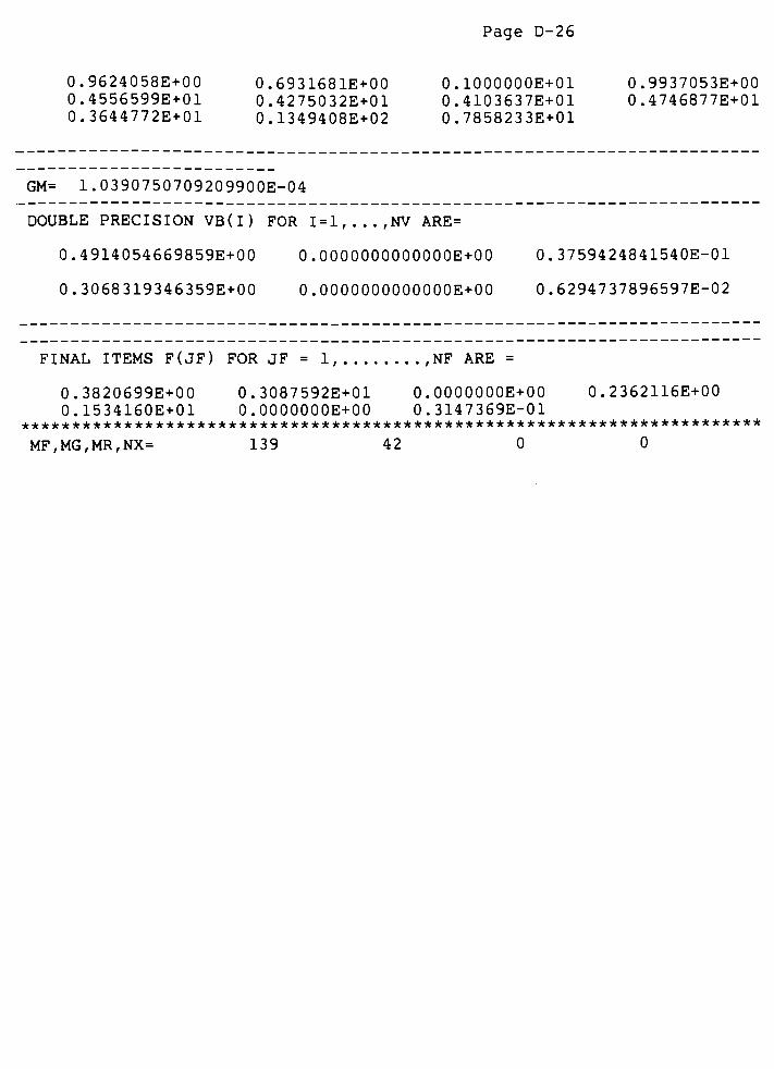
Page D-26
0.9624058E+00 0 . 6931681E+00 0 . lOOOOOOE+01 0 . 9937053E+00
0.4556599E+01 0 . 4275032E+01 0 . 4103637E+01 0 . 4746877E+01
0.3644772E+01 0 . 1349408E+02 0 . 7858233E+01
GM= 1.0390750709209900E-04
DOUBLE PRECISION VB(I) FOR 1=1,..., NV ARE=
0.4914054669859E+00 0 . 0000OO0OOO000E+OO 0 . 3759424841540E-01
0.3068319346359E+00 0 . 0000000000000E+00 0 . 6294737896597E-02
FINAL ITEMS F(JF) FOR JF = 1, ,NF ARE =
0.3820699E+00 0 . 3087592E+01 O.OOOOOOOE+00 0 . 2362116E+00
0.1534160E+01 0.0000000E+00 0 . 3147369E-01************************************************************************
MF,MG,MR,NX= 139 42 0 0

Page D-27
*************************************************************************
*
* THIS IS THE FORTRAN VERSION OF THE MODSER PROGRAM *
* " AOD."
THIS VERSION (6/6/84) HAS BEEN MODIFIED FOR USE ON A* VAX/VMS 11/782 DIGITAL COMPUTER. *
*A
*DR. R. C. JOHNSON, PHD., P.E. *
**
***********************SUBROUTINES USED ****************************
* *
* 1) ANALYSIS *
*: CALCULATES THE VALUE OF THE PENALIZED OPTIMIZATION *
*QUANTITY, REGIONAL CONSTRAINTS, AND EQUALITY CON- *
*STRAINTS. *
* *
* 2) FBPRINT *
*: PERFORMS A FULL BASEPOINT PRINTOUT. *
* *
* 3) GRADIENT *
*: APPROXIMATES THE GRADIENT VECTOR, g, BY FINITE *
* DIFFERENCES. *
* *
* 4) INPUTPO *
*'
: GIVES A PRINTOUT OF THE INPUT DATA. *
* *
* 5) LSEARCH *
*: CONTROL OF LINE SEARCH BY FDAP TECHNIQUE; ALSO *
* PERFORMS CP CALCULATION BY SELF TUNING. *
* *
* 6) MBPRINT*
*: PERFORMS A MINIMAL BASEPOINT PRINTOUT .
*
* *
* 7) NEWBP*
*: PROVIDES A NEWBASE POINT FOR THE SEARCH. *
* *
* 8) PRINT(L)*
*: PROVIDES A LINE OF CHARACTERS IN THE PRINTOUT AS *
* DETERMINED BY THE CHOICE OF L .
*
**
* 9) SDIR*
*: DETEMINES THE SEARCH DIRECTION
, s, USING EITHER *
*
*
MSD OR GCG TECHNIQUES.*
**
* 10) SGSEARCH*
* RANDOM GENERATION OF A GOOD STARTING POINT. *
*
'
*
* 11) STORINDEX*
* PROVIDES A STROAGE AND INDEXING OPERATION .
*
*
*
*
****************** SUBFUNCTIONS USED*********************************
**
* i) sgn(p)*
* : RETURNS EITHER A "+l","-l",OR"0"
DEPENDING UPON *

*
*
*
*
*
*
Page D-28
THE SIGN OF P.
2)RND(SEED)
: RETURNS
SEED.
A RANDOM NUMBER BASED UPON A USER CHOOSEN
*
*
*
*
*
*
************************************************************************
*MAIN PROGRAM FOLLOWS
*
************************************************************************
*
25
PARAMETER (MAXN = 32)REAL * 8 C(MAXN) ,CD(MAXN) ,CG(MAXN) ,CN(MAXN) ,CS(MAXN) ,CX(MAXN) ,
Sc DN(MAXN) ,DP(MAXN) ,DV(MAXN) ,E(MAXN) ,EA(MAXN) ,EB(MAXN) ,
& F(MAXN) ,G(24) ,GA(3) ,GB(MAXN) ,GC(MAXN) ,GS(MAXN) ,11(10) ,
& MI (10) ,OA(MAXN) ,OD(MAXN) ,OE(MAXN) ,OF(MAXN) ,OG(MAXN) ,
Sc OI(MAXN) ,OK(MAXN) ,OS(MAXN) ,PI(10) ,R(MAXN) ,RA(MAXN) ,
& RB(MAXN) ,RR(19) ,RS(MAXN) ,S(MAXN) ,SA(MAXN) ,SB(MAXN) ,
Sc SC(MAXN) ,SD(MAXN) ,SE(MAXN) ,SF(MAXN) ,SK(MAXN) ,TB(MAXN) ,
S. U(MAXN) ,UA(MAXN) ,UB(MAXN) ,V(MAXN) ,VA(MAXN) ,VB(MAXN) ,
& VD(MAXN) ,VE(MAXN) ,VF(MAXN) ,VG(MAXN) ,VU(MAXN) ,YD(MAXN) ,
& YE(MAXN) ,YF(MAXN) ,YS(MAXN) ,ZZ(24) , AOIDRS , AOIDMX, A03DRS ,
& AO 3DMX,A,AB
, AC ,AD
,AE
, AG ,AL
,AM
,AP , AW , AR , AT , B ,
BA ,BB
, CA ,
& CL,CP
,CF
,DB
, DC ,DD
,DL
,DS
,DT
,FB ,
FD,FE
,FH
, FM ,FP , FR , FS ,
& F21MAX,F21RMS,F32MAX,F32RMS,F41MAX,F41RMS,F4 3MAX,& F4 3RMS
,FSHMAX
, FSHRMS ,FT , FX ,
GM, GN ,
GU , GV , GW , GX ,GY , GZ , H ,
& HA,HB
, OU ,OV , OW ,
P,PA
,PB
, PG , Q ,QA
,QB
,QD
,QE
,QF , QG , RM ,
SEED,
& TDMAX,TDRMS
,W ,
WA,WB
,WD
,WE
,WF
,WK
,X,XA
,XB
,XD
,XE
,XF
,XG , X I ,
Sc X3,YJ,YM
INTEGER * 4 N(MAXN) ,NA(MAXN) ,NB (MAXN) ,NC(MAXN) ,NS (MAXN) ,
QUIT,
& I D,IT
,J ,JT
,JX
,K
,KA
, KC ,KE
,KG
,KK
,KP
,KT
,KX
,LZZ , MD ,
& ME ,MF
, MG ,MN
,MR
,MS
,MX
,ND
,NE
,NF
, NG ,NN
,NP
,NR
,NRMS
, NU ,
& NV,NX
COMMON G ,ZZ
, RR, AP ,FSHMAX
,F2 1MAX
,D32MAX
,F4 1MAX
,F4 3MAX
,AOIDMX
,
Sc A03DMX,TDMAX
,FSHRMS ,
F21RMS,F32RMS ,
F4 1RMS,F4 3RMS , AOIDRS ,
Sc A03DRS,TDRMS/A1 /NRMS, NUC, NGQ, NR
WRITE(4,*)
WRITE(4,*)
WRITE (6,*)
WRITE (6,*)
WRITE(6,*)
WRITE(6,*)
WRITE(6,*)
WRITE(6,*)
WRITE(6,*)
WRITE(6,*)
WRITE(6,*)
WRITE(6,*)
WRITE(6,*)
WRITE(6,*)
WRITE(6,*)
WRITE (6,*)
WRITE(6,*)
WRITE(6,*)
WRITE(6,*)
MODSER - AOD FORTRAN VERSION(6/6/84)'
APPLICATION : BALANCING OF FOUR BARMECHANISMS'
***************************************
MODSER- P519RE FORTRAN VERSION FOLLOWS (6/6/84)
APPLICATION : BALANCING OF FOUR BARMECHANISMS'
**************************************'
OUTPUT IS PROVIDED ON THE FOLLOWING:'
**************************************'
FOR004
FOR006
FOR007
AOD SEARCHPROCESS'
SUMMARY OF FINALRESULTS'
SUMMARY OF FINALRESULTS'
y^************************************************1
FOR00 9- FOR017 IS FOR PLOTTING THE FINAL
RESULTS'
XX************************************************'
FOR00 9
FOR010
FOR011
FOR012
FOR013
CRANK ANGLE FROM 1-360DEGREES'
FORCE F21 FOR EACH CRANKANGLE'
FORCE F32 FOR EACH CRANKANGLE'
FORCE F41 FOR EACH CRANKANGLE'
FORCE F4 3 FOR EACH CRANKANGLE'

Page D-29
27
MOMENT MSHOl FOR EACH CRANK ANGLE
MOMENT MSH03 FOR EACH CRANK ANGLE
FORCE FSH FOR EACH CRANKANGLE'
INPUT TORQUE FOR EACH CRANKANGLE'
P519RE FORTRAN VERSION
: BALANCING OF FOUR
DATA FILE FORTHTO1
WRITE(6,*)'
FOR014WRITE (6,*)' FOR015WRITE (6,*)' FOR016WRITE (6,*)' FOR017WRITE (6,*)WRITE (7,*) 'MODSER -
WRITE (7,*) 'APPLICATIONWRITE(9,*) 'THIS IS A
WRITEUO,*) 'THIS IS A DATA
WRITE(11,*) 'THIS IS A DATA
WRITEU2,*) 'THIS IS A DATA
WRITE(13,*) 'THIS IS A DATA
WRITE(14,*) 'THIS IS A DATA
WRITE (15,*) 'THIS IS A DATA
WRITEU6,*) 'THIS IS A DATA
WRITEU7,*) 'THIS IS A DATA
CALL PRINT(O)
WRITE(4,*) 'INPUT DATA:*
AP = 4.0*ATAN (1.0)AR = 57.29578
0.
0
= 0
AB,AE,AG,AL,AM,AW,AT,CA,CL,CF,JX,KX/10.,.5,1.E03,1.E05,8._,.,
_
2. E04, 2. ,.85, .25, .25, 300, 250/
READ(3,*)KC,KG,MD,MN,MS,MX,ND,NE,NF,NG,NP,NR,NU,NV,NRMS,NUC, NGQ, SEED
FILE
FILE
FILE
FILE
FILE
FILE
FILE
FILE
FOR
FOR
FOR
FOR
FOR
FOR
FOR
FOR
FINAL
FINAL
FINAL
FINAL
FINAL
FINAL
FINAL
FINAL
FOLLOWS (6/6/84)BAR
MECHANISMS'
F21*
F32'
F41'
F43'
-AOID*
-A03D'
FSH'
TD'
CP =
KP =
QUIT
DATA
READ ( 3
READ (3
IF (NG
ENDIF
IF (MX
*)
.*)
,NE
(CN(I)
(CX(I)
0)
1= 1,NV)1= 1,NV)
LE.0)
THEN
READ ( 3
THEN
READ ( 3
ENDIF
IF (NRMS
ENDIF
;) (CG(I) ,I=1,NG)
:) (CS(I) ,1= 1,NV)
EQ.l) THEN
CALL PGAUSS (NGQ)
*
**
*
SPECIFIED START POINT DATA (CASE OF NO SG) **
IF (MS.NE.0) THEN
READ(3,*) (OS(lS),IS = 1,MS)
ENDIF
IF (KC.EQ.0) THEN
GO TO 3 3
ENDIF
*USER PROGRAMS EQUATIONS FOR CALCULATED CONSTANTS C(IC), (IC=1 TO KC) *
*
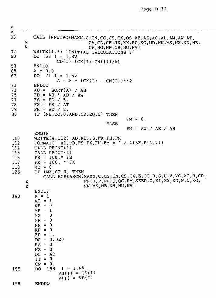
Page D-30
* :
33 CALL INPUTPO(MAXN,C,CN,CG,CS,CX,OS,AB,AE,AG,AL,AM,AW,AT,& CA
,CL
,CF
,JX
,KX
, KC , KG ,MD
, MN ,MS ,MX
,ND
,NE
,
& NF,NG,NP,NR,NU,NV)
37 WRITE(4,*)'
INITIAL CALCULATIONS:'
50 DO 53 I = 1,NV
CD(I)=(CX(I)-CN(I))/AL
53 ENDDO
65 A = 0.0
67 DO 71 I = 1,NV
A = A + (CX(I) -
CN(I) )**2
71 ENDDO
73 AD = SQRT(A) / AB
75 FD = AB * AD / AW
77 FS = FD / 5.
78 FX = FS / AT
79 FH = AD / 2.
80 IF (NE.EQ.0.AND.NR.EQ.0) THEN
FM = 0.
ELSE
FM = AW / AE / AB
ENDIF
110 WRITE(4,112) AD,FD,FS,FX,FH,FM
112FORMAT('
AD,FD,FS,FX,FH,FM ='
, / , 4 ( 3X, E14 . 7 ) )
114 CALL PRINT(l)
115 CALL PRINT(l)
116 FS = 100.* FS
117 FX = 100. * FX
118 ME = 0
125 IF (MX.GT.0) THEN
CALL SGSEARCH (MAXN,C,CG ,
CN,CS
,CX
,E
,O I
,R
, S , U ,V, VG ,
AG,B
,CP
,
Sc FP,H ,
P , PG , Q ,QG ,
RM,SEED
,X
,X I
, X3 , XG ,W ,
N,KG ,
Sc MN,MX,NE,NR,NU,NV)
ENDIF
140 K = 1
KT = 1
KE = 0
MF = 1
MG = 0
MR = 0
NN = 0
KP = 0
FP = 1.
DC = 0.0E0
KA = 0
NX = 0
DL = AD
IT = 0
CP = 0.
155 DO 158 I = 1,NV
VB(I) = CS(I)
V(I) = VB(I)
158 ENDDO
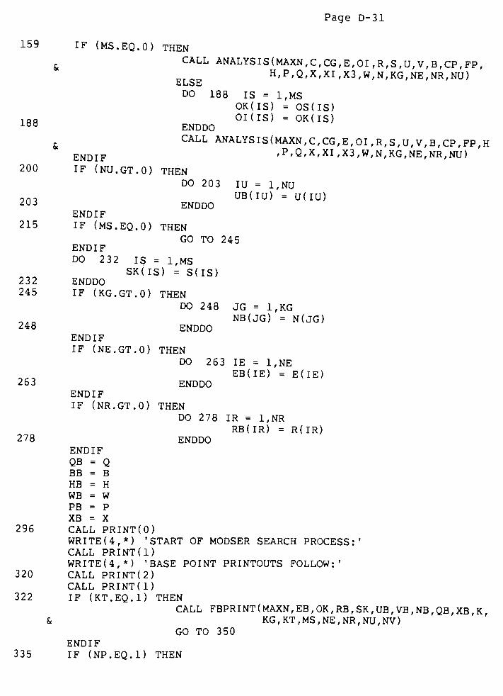
Page D-31
159 IF (MS.EQ.O) THEN
&CALL ANALYSIS(MAXN,C,CG,E,OI,R,S,U,V,B,CP,FP,
___,H,P,Q,X,XI,X3,W,N,KG,NE,NR,NU)
ELSE
DO 188 IS = 1,MS
OK(IS) = OS(IS)Tap- OI(IS) = OK(IS)10
ENDDO
&CALL ANALYSIS(MAXN,C,CG,E,OI,R,S,U,V,B,CP,FP,H
ENDIF /p,Q,X,XI,X3,W,N,KG,NE,NR,NU)
200 IF (NU.GT.O) THEN
DO 203 IU = 1,NU
9n., UB(IU) = U(IU)ZU6
ENDDOENDIF
215 IF (MS.EQ.O) THEN
GO TO 245ENDIF
DO 232 IS = 1,MS
SK(IS) = S(IS)232 ENDDO
245 IF (KG.GT.O) THEN
DO 248 JG = 1,KG
NB(JG) = N(JG)248 ENDDO
ENDIF
IF (NE.GT.O) THEN
DO 263 IE = 1,NE
EB(IE) = E(IE)263 ENDDO
ENDIF
IF (NR.GT.O) THEN
DO 278 IR = 1,NR
RB(IR) = R(IR)278 ENDDO
ENDIF
QB = QBB = B
HB = H
WB = W
PB = P
XB = X
296 CALL PRINT(O)
WRITE (4,*) 'START OF MODSER SEARCHPROCESS:'
CALL PRINT(l)
WRITE (4,*) 'BASE POINT PRINTOUTSFOLLOW:'
320 CALL PRINK 2)
CALL PRINT(l)
322 IF (KT.EQ.l) THEN
CALL FBPRINT (MAXN, EB ,OK
, RB ,SK
, UB , VB , NB , QB , XB , K ,
Sc KG ,KT
, MS, NE , NR , NU , NV )
GO TO 3 50
ENDIF
335 IF (NP.EQ.l) THEN
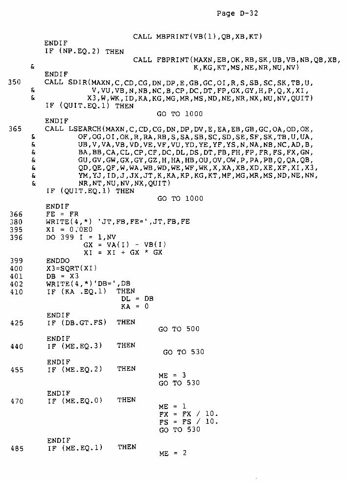
Page D-32
CALL MBPRINT(VBQ) ,QB,XB,KT)
ENDIF
IF (NP.EQ.2) THEN
CALL FBPRI NT (MAXN,EB , OK ,
RB,SK
,UB
,VB ,
NB, QB ,
XB,
& K,KG,KT,MS,NE,NR,NU,NV)
ENDIF
350 CALL SDIR(MAXN,C,CD,CG,DN,DP,E,GB,GC,OI,R,S,SB,SC,SK,TB,U,& V
, VU , VB , N ,NB
, NC ,B,CP
, DC ,DT , FP , GX ,
GY,H, P , Q ,
X,XI
,
S. X3,W,WK, ID,KA,KG,MG,MR,MS,ND,NE,NR,NX,NU,NV,QUIT)
IF (QUIT.EQ.l) THEN
GO TO 1000
ENDIF
365 CALL LSEARCH(MAXN,C,CD,CG,DN,DP,DV,E,EA,EB,GB,GC,OA,OD,OE,Sc OF , OG , 0 1
, OK ,R,RA
, RB , S ,SA , SB , SC ,
SD,SE
,SF
,SK
,TB , U ,
UA,
Sc UB , V ,VA
, VB , VD , VE ,VF
, VU , YD ,YE
,YF
, YS ,N,NA
,NB
, NC ,AD
,B,
Sc BA,BB
,CA
, CL ,CP
,CF
, DC ,DL
, DS ,DT
,FB
,FH
,FP
,FR
,FS ,
FX,GN ,
Sc GU,GV,GW,GX,GY,GZ,H,HA,HB,OU,OV,OW,P,PA,PB,Q,QA,QB,Sc QD , QE , QF , W , WA , WB , WD
,WE
,WF
,WK , X ,
XA,XB
,XD
,XE
,XF
,X I
, X3 ,
Sc YM,YJ , ID , J ,
JX,JT
,K,KA
,KP
, KG , KT ,MF ,MG , MR , MS , ND ,NE
,NN
,
Sc NR,NT,NU,NV,NX,QUIT)
IF (QUIT.EQ.l) THEN
GO TO 1000
ENDIF
366 FE = FR
330 WRITE(4,*)' JT,FB,FE='
,JT,FB,FE
395 XI = 0/0E0
396 DO 399 I = 1,NV
GX = VA(I)-
VB(I)
XI - XI + GX * GX
399 ENDDO
400 X3=SQRT(XI)
401 DB = X3
402 WRITE (4,*)'DB=
'
,DB
410 IF (KA .EQ.l)THEN
DL = DB
KA = 0
ENDIF
425 IF (DB.GT.FS) THEN
ENDIF
440 IF (ME.EQ.3) THEN
ENDIF
455 IF (ME.EQ.2) THEN
ENDIF
470 IF (ME.EQ.0) THEN
GO TO 500
GO TO 530
ME = 3
GO TO 530
ME = 1
FX = FX / 10
FS = FS / 10
GO TO 530
ENDIF
485 IF (ME. EQ.l) THEN
ME = 2
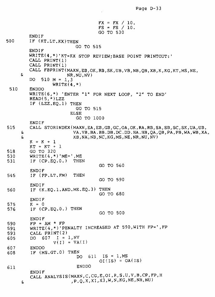
Page D-33
FX = FX / 10.
FS = FS / 10.
GO TO 530
ENDIF
500 IF (KT.LT.KX)THEN
GO TO 515
ENDIF
WRITE(4,*) 'KT=KX STOP REVIEW;BASE POINTPRINTOUT:'
CALL PRINT(l)
CALL PRINT (1)CALL FBPRINT (MAXN
,EB
,OK
,RB
,SK
,UB
, VB ,NB
,QB
,XB
,K
, KG ,KT
, MS ,NE
,
& NR, NU , NV )
DO 510 M = 1,3
WRITE (4,*)510 ENDDO
WRITE (6,*) 'ENTER"1"
FOR NEXT LOOP,"2"
TOEND'
READ(5,*)LZZ
IF (LZZ.EQ.l) THEN
GO TO 515
ELSE
GO TO 1000
ENDIF
515 CALL STORINDEX (MAXN,EA
,EB
,GB
, GC ,OA
,OK
,RA
,RB
,SA
,SB
,SC
,SK
,UA
,UB
,
Sc VA . VB , BA . BB . DB , DC . DD . HA , HB ,QA
,QB
,PA
,PB
, WA ,WB
, XA.,Sc XB
, NA", NB , NC , KG , MS ,NE
,NR
, NU ,NV )
K = K + 1
KT = KT + 1
518 GO TO 320
530 WRITE(4,*)'ME='
,ME
531 IF (CP.EQ.0.) THEN
ENDIF
545 IF (FP.LT.FM) THEN
GO TO 560
GO TO 590
ENDIF
560 IF (K.EQ.1.AND.ME.EQ.3) THEN
GO TO 680
ENDIF
575 K = 0
576 IF (CP.EQ.0.) THEN
GO TO 500
ENDIF
590 FP = AM* FP
591 WRITE(4,*) 'PENALTY INCREASED AT 590,WITH FP=',FP
593 CALL PRINT(2)
605 DO 607 I = 1,NV
V(I) = VA(I)
607 ENDDO
608 IF (MS.GT.0) THEN
DO 611 IS = 1,MS
OI(IS) = OA(IS)
611 ENDDO
ENDIF
CALL ANALYSIS (MAXN, C , CG, E,OI , R, S ,U ,V,B
,CP
, FP ,H
Sc
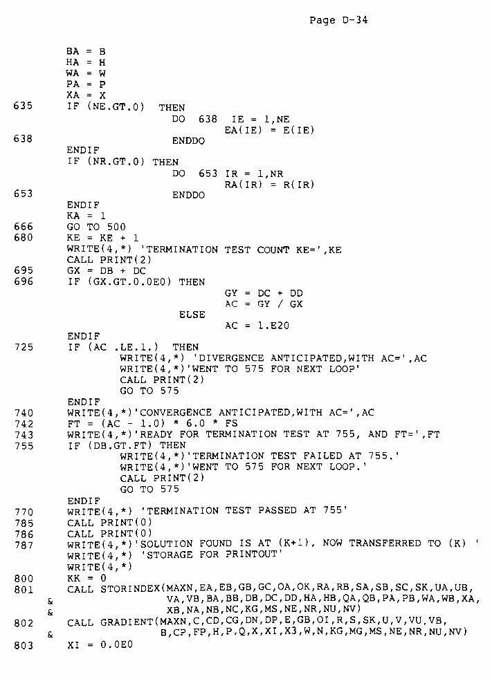
Page D-34
BA = B
HA = H
WA = W
PA = P
XA = X
635 IF (NE.GT.O) THEN
DO 638 IE = 1,NE
EA(IE) = E(IE)638 ENDDO
ENDIF
IF (NR.GT.O) THEN
DO 653 IR = 1,NR
RA(IR) = R(IR)653 ENDDO
ENDIF
KA = 1
666 GO TO 500
680 KE = KE + 1
WRITE(4,*) 'TERMINATION TEST COUNT KE=',KE
CALL PRINT(2)
695 GX = DB + DC
696 IF (GX.GT.0.0E0) THEN
770
785
786
787
800
801
Sc
Sc
802
Sc
803
GY = DC + DD
AC = GY / GX
AC = 1.E20
ELSE
ENDIF
725 IF (AC .LE.l.) THEN
WRITE(4,*) 'DIVERGENCE ANTICIPATED,WITH AC=',AC
WRITE (4,*) 'WENT TO 575 FOR NEXTLOOP'
CALL PRINT(2)
GO TO 575
ENDIF
740 WRITE(4,*) 'CONVERGENCE ANTICIPATED,WITH AC=',AC
742 FT = (AC - 1.0) * 6.0 * FS
743 WRITE (4,*) 'READY FOR TERMINATION TEST AT 755, AND FT= '
, FT
7 55 IF (DB.GT.FT) THEN
WRITE( 4,*) 'TERMINATION TEST FAILED AT755.'
WRITE (4,*) 'WENT TO 575 FOR NEXTLOOP."
CALL PRINT(2)
GO TO 575
ENDIF
WRITE(4,*) 'TERMINATION TEST PASSED AT755'
CALL PRINT(O)
CALL PRINT(O)
WRITE(4,*) 'SOLUTION FOUND IS AT (K+1), NOW TRANSFERRED TO (K)'
WRITE (4,*) 'STORAGE FORPRINTOUT'
WRITE(4,*)
KK = 0
CALL STORINDEX ( MAXN,EA
,EB
,GB
,GC ,
OA ,OK
,RA
,RB
, SA ,SB
, SC ,SK
,UA
, UB ,
VA,VB ,
BA ,BB
,DB
,DC
,DD
,HA
,HB
,QA
, QB ,PA
, PB , WA,WB
,XA
,
XB,NA,NB,NC,KG,MS,NE,NR,NU,NV)
CALL GRADIENT (MAXN, C, CD, CG,DN, DP, E,GB ,01 , R, S , SK,U , V, VU ,VB
,
B,CP,FP,H,P,Q,X,XI,X3,W,N,KG,MG,MS,NE,NR,NU,NV)
XI = 0.0E0
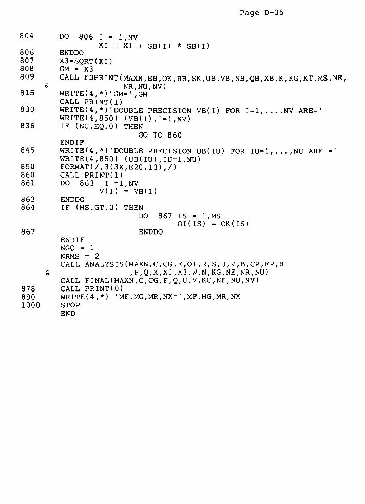
Page D-35
804 DO 806 I = 1,NV
XI = XI + GB(I) * GB(I)806 ENDDO
807 X3=SQRT(XI)808 GM = X3
809 CALL FBPRINT(MAXN,EB,OK,RB,SK,UB,VB,NB,QB,XB,K,KG,KT,MS,NE,& NR
, NU , NV )815 WRITE(4,*)
'GM='
,GM
CALL PRINT(l)
830 WRITE (4,*) 'DOUBLE PRECISION VB(I) FOR 1=1,..., NV ARE='
WRITE(4,850) ( VB( I ) , 1=1 ,NV)836 IF (NU.EQ.0) THEN
GO TO 860
ENDIF
845 WRITE (4,*) 'DOUBLE PRECISION UB(IU) FOR IU=1,...,NU ARE='
WRITE(4,850) (UB( IU) , IU=1 ,NU)
850 FORMAT(/,3(3X,E20.13),/)860 CALL PRINT(l)
861 DO 863 I =1,NV
V(I) = VB(I)
863 ENDDO
864 IF (MS.GT.0) THEN
DO 867 IS = 1,MS
OI(IS) = OK(IS)
867 ENDDO
ENDIF
NGQ = 1
NRMS = 2
CALL ANALYS I S ( MAXN ,C,CG,E,OI,R,S,U,V,B,CP,FP,H
Sc ,P,Q,X,XI,X3,W,N,KG,NE,NR,NU)
CALL F INAL (MAXN,C , CG ,
F, Q ,
U,V, KC ,
NF,NU ,
NV )
878 CALL PRINT(O)
890 WRITE(4,*) 'MF,MG,MR,NX= '
,MF,MG,MR,NX
1000 STOP
END
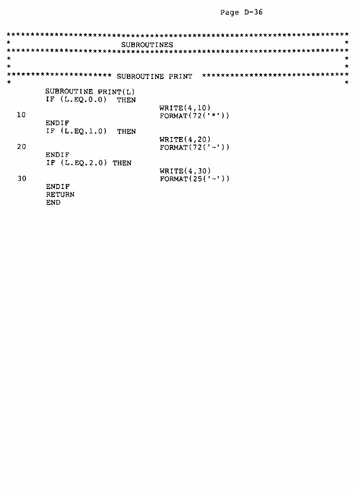
Page D-36
************************************************************************
*SUBROUTINES
**************************************************************
*
*
********************** SUBROUTINE PRINT*******************************
* *
**********
*
*
10
20
30
SUBROUTINE PRINT (L)IF (L.EQ.0.0) THEN
ENDIF
IF (L.EQ.1.0) THEN
ENDIF
IF (L.EQ.2.0) THEN
ENDIF
RETURN
END
WRITE (4, 10)FORMAT ( 72 (
'*'
))
WRITE(4,20)
FORMAT ( 7 2 ('-
'
) )
WRITE(4,30)
FORMAT ( 25 ('-'
) )

Page D-37
* *
*******************NEW BASE POINT SUBROUTINE *************************
* *
SUBROUTINE NEWBP (MAXN, C , CG ,
E,EB,OI,OK, R,RB, S , SK,U,UB ,V, VB, B, BB,
& CP,FP,H,HB,P,PB,Q,QB,W,WB,X,XI,X3,XB,N,NB,KG,MS
&,NU,NE,NR,NV)
REAL * 8 C(MAXN) ,CG(MAXN) ,E(MAXN) ,EB(MAXN) ,0I(MAXN) ,OK(MAXN) ,
& R(MAXN) ,RB(MAXN) ,S(MAXN) ,SK(MAXN) ,U(MAXN) ,UB(MAXN) ,
& V(MAXN) ,VB(MAXN) , B, BB,CP, FP , H,HB, P, PB,Q,QB,W,WB,X,XI,
Sc X3,XB
INTEGER * 4 N(MAXN) ,NB(MAXN) , KG,MS ,NU, NE ,NR,NV
1090 DO 1107 I = 1,NV
V(I) = VB(I)
1107 ENDDO
IF (MS.GT.O) THEN
DO 1111 IS = 1,MS
OI(IS) = OK(IS)
1111 ENDDO
ENDIF
CALL ANALYS I S (MAXN ,C,CG,E,OI,R,S,U,V,B,CP,FP,H
Sc ,P,Q,X,XI,X3,W,N,KG,NE,NR,NU)
QB = QBB = B
HB = H
WB = W
PB =
P"
XB = X
IF (NU.GT.O) THEN
DO 1130 IU = 1,NU
UB(IU) = U(IU)
1130 ENDDO
ENDIF
IF (MS.GT.O) THEN
DO 1138 IS = 1,MS
SK(IS) = S(IS)
1138 ENDDO
ENDIF
IF (NE.GT.0) THEN
DO 1153 IE = 1,NE
EB(IE) = E(IE)
1153 ENDDO
ENDIF
IF (NR.GT.0) THEN
DO 1168 IR = 1,NR
RB(IR) = R(IR)
1168 ENDDO
ENDIF
IF (KG.GT.0) THEN
DO 1183 JG = 1,KG
NB(JG) = N(JG)
1183 ENDDO
ENDIF
RETURN
END
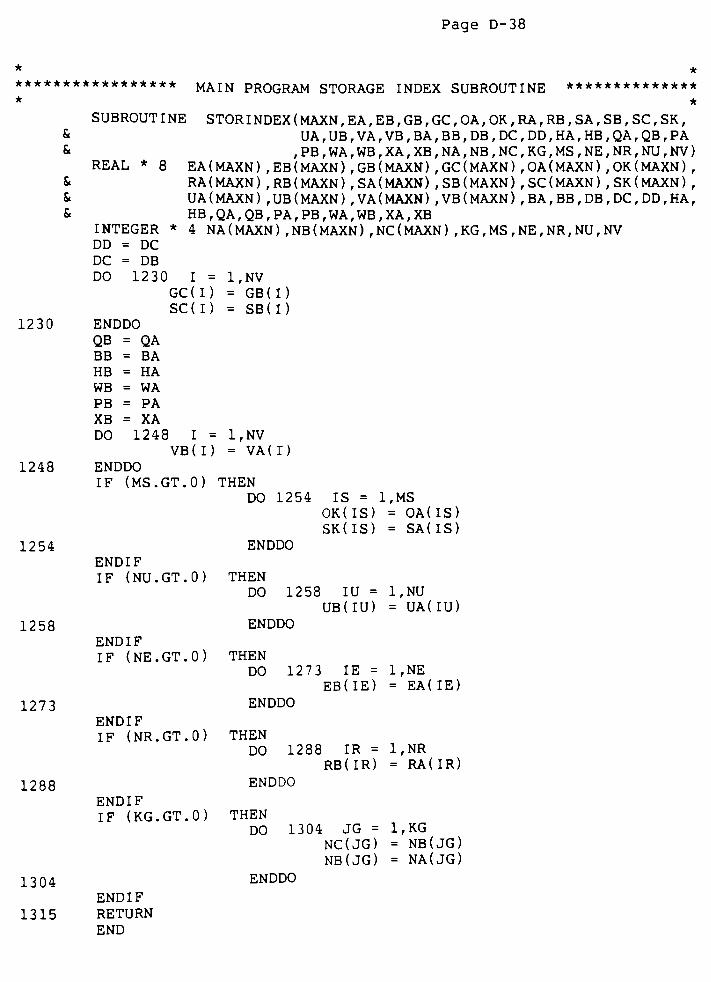
Page D-38
* *
*****************MAIN PROGRAM STORAGE INDEX SUBROUTINE **************
* *
SUBROUTINE STOR INDEX (MAXN, EA, EB,GB,GC,OA, OK,RA,RB , SA, SB, SC, SK,& UA
, UB ,VA
,VB ,
BA,BB
,DB , DC ,
DD,HA
,HB ,
QA,QB
, PA
&,PB,WA,WB,XA,XB,NA,NB,NC,KG,MS,NE,NR,NU,NV)
REAL * 8 EA(MAXN) ,EB(MAXN) ,GB(MAXN) ,GC(MAXN) ,OA(MAXN) ,OK(MAXN) ,
& RA(MAXN) ,RB(MAXN),SA(MAXN) ,SB(MAXN) , SC(MAXN) ,SK(MAXN) ,
& UA(MAXN) ,UB(MAXN) ,VA(MAXN) ,VB(MAXN) , BA, BB ,DB
, DC, DD,HA,Sc HB,QA,QB,PA,PB,WA,WB,XA,XB
INTEGER * 4 NA(MAXN) ,NB(MAXN) ,NC(MAXN) , KG, MS ,NE, NR,NU,NV
DD = DC
DC = DB
DO 1230 I = 1,NV
GC(I) = GB(I)
SC(I) = SB(I)
1230 ENDDO
QB = QA
BB = BA
HB = HA
WB = WA
PB = PA
XB = XA
DO 1248 I = 1,NV
VB(I) = VA(I)
1248 ENDDO
IF (MS.GT.O) THEN
DO 1254 IS = 1,MS
OK(IS) = OA(IS)
SK(IS) = SA( IS)
1254 ENDDO
ENDIF
IF (NU.GT.O) THEN
DO 1258 IU = 1,NU
UB(IU) = UA(IU)
1258 ENDDO
ENDIF
IF (NE.GT.O) THEN
DO 1273 IE = 1,NE
EB(IE) = EA(IE)
127 3 ENDDO
ENDIF
IF (NR.GT.O) THEN
DO 1288 IR = 1,NR
RB(IR) = RA(IR)
1288 ENDDO
ENDIF
IF (KG.GT.O) THEN
DO 1304 JG = 1,KG
NC(JG) = NB(JG)
NB(JG) = NA(JG)
1304 ENDDO
ENDIF
1315 RETURN
END

Page D-39
**
***********************RAND0M START poiNT SUBROUTINE *****************
**
SUBROUTINE SGSEARCH (MAXN,C,CG,CN,CS , CX,E ,01 ,R, S ,U,V, VG,AG, B,CP,& FP
, H ,P, PG , Q , QG ,
RM,SEED
,X , X I , X3 , XG ,
W ,N, KG ,
& MN,MX,NE,NR,NU,NV)REAL * 8 C(MAXN) ,CG(MAXN),CN(MAXN),CS(MAXN) ,CX(MAXN) ,E(MAXN) ,
& Ol(MAXN),R(MAXN),S(MAXN),U(MAXN),V(MAXN) ,VG(MAXN) ,AG,
& B,CP,FP,H,P,PG,Q,QG,RM,SEED,X,XI,X3,XG,WINTEGER * 4 N(MAXN) ,KG,KS ,MN,MX,NE,NR,NU,NV
KS = 1
XG = 1.E19
CP = AG
FP = 1.
2014 DO 2017 I = 1,NV
RM=RND(SEED)
V(I) = CN(I) + RM * (CX(I) -
CN(I))
SEED = RM
2017 ENDDO
CALL ANALYS I S (MAXN ,C,CG,E,OI,R,S,U,V,B,CP,FP,H
Sc,P,Q,X,XI,X3,W,N,KG,NE,NR,NU)
2030 IF (X.LT.XG) THEN
XG = X
QG = QPG = P
DO 2036 I = l.NV
VG(I) = V(I)
2036 ENDDO
ENDIF
IF (KS.LT.MN) THEN
GO TO 2075
ENDIF
2060 IF (PG.EQ.0.) THEN
GO TO 2090
ENDIF
2075 IF (KS.LT.MX) THEN
KS = KS + 1
GO TO 2014
ENDIF
2090 WRITE(4,*)
WRITE (4,*) 'SG SEARCH GAVE FOLLOWINGPOINT:*
WRITE(4,*)
2096 WRITE(4,*) 'QG, PG,X :',QG,PG,XG
WRITE(4,*)
2105 WRITE(4,*)'VG(I) FOR 1=1, . . . ,
NV ARE='
WRITE(4,2130)(VG(I) ,I=1,NV)
WRITE(4,*)
2130 F0RMAT(/,4(4X,E14.7) )
2135 DO 2137 I = 1,NV
CS(I) = VG(I)
2137 ENDDO
WRITE(6,*) 'STARTING POINT OBTAINED BY SGSEARCH'
WRITE(6,*) (VG(I),I=1,NV)
2138 RETURN
END
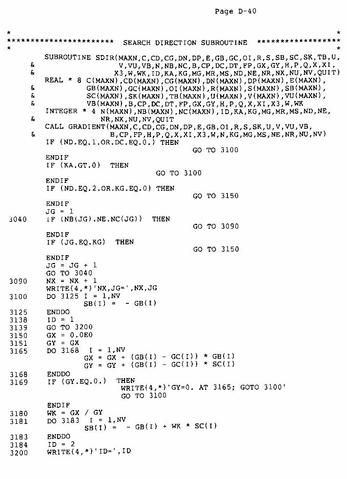
Page D-40
* *
***********************SEARCH DIRECTION SUBROUTINE
******************
* *
SUBROUTINE SDIR(MAXN,C,CD,CG, DN,DP,E, GB,GC,OI , R, S , SB, SC, SK,TB,U,& V,VU,VB,N,NB,NC,B,CP,DC,DT,FP,GX,GY,H,P,Q,X,XI,
& X3,W,WK,ID,KA,KG,MG,MR,MS,ND,NE,NR,NX,NU,NV,QUIT)
REAL * 8 C(MAXN) ,CD(MAXN) ,CG(MAXN) ,DN(MAXN) ,DP(MAXN) ,E(MAXN) ,
Sc GB(MAXN) ,GC(MAXN) ,01 (MAXN) ,R(MAXN) ,S(MAXN) ,SB(MAXN) ,
& SC(MAXN) ,SK(MAXN) ,TB(MAXN) ,U(MAXN) ,V(MAXN) ,VU(MAXN) ,
Sc VB(MAXN) ,B,CP,DC,DT,FP,GX,GY,H,P,Q,X,XI,X3,W,WK
INTEGER * 4 N(MAXN) ,NB (MAXN) ,NC(MAXN) ,ID,KA,KG,MG ,MR,MS ,ND,
NE ,
Sc NR,NX,NU,NV,QUIT
CALL GRAD I ENT (MAXN, C , CD , CG ,
DN,DP
,E,GB
,0 I ,
R, S ,
SK, U , V ,
VU ,VB
,
Sc B , CP ,FP , H , P , Q ,
X,X I
,X3 , W ,
N, KG , MG , MS ,
NE ,NR , NU ,
NV )
IF (ND.EQ.l.OR.DC.EQ.O.) THEN
GO TO 3100
ENDIF
IF (KA.GT.O) THEN
GO TO 3100
ENDIF
IF (ND.EQ.2.OR.KG.EQ.0) THEN
GO TO 3150
ENDIF
JG = 1
3040 IF (NB(JG) .NE.NC(JG) ) THEN
GO TO 3090
ENDIF
IF (JG.EQ.KG) THEN
GO TO 3150
ENDIF
JG = JG + 1
GO TO 3040
3090 NX = NX + 1
WRITE ( 4 ,
* )'NX
,JG=
'
,NX
,JG
3100 DO 3125 I = 1,NV
SB ( I ) = - GB ( I )
3125 ENDDO
3138 ID = 1
3139 GO TO 3200
3150 GX = 0.0E0
3151 GY = GX
3165 DO 3168 I = 1,NV
GX = GX + (GB(I) - GC(I))* GB(I)
GY = GY + (GB(I) - GC(D)* SC(l)
3168 ENDDO
3169 IF (GY.EQ.0.) THEN
WRITE(4,*) *GY=0. AT 3165; GOTO3100'
GO TO 3100
ENDIF
3180 WK = GX / GY
3181 DO 3183 I = 1,NV
SB(I) =" GB(I) + WK * SC(I)
318 3 ENDDO
3184 ID = 2
3200 WRITE(4,*)' ID='
,ID
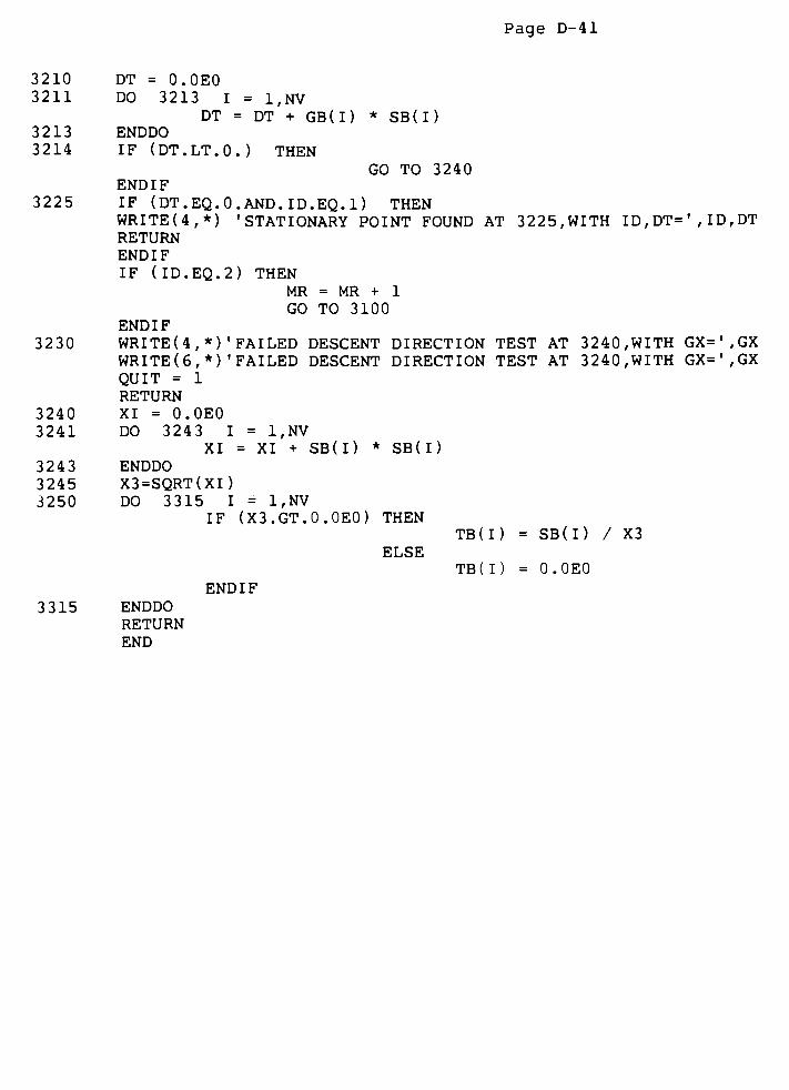
Page D-41
3210 DT = 0.0E0
3211 DO 3213 I = 1,NV
DT = DT + GB(I) * SB(I)
3213 ENDDO
3214 IF (DT.LT.O.) THEN
GO TO 3240
ENDIF
3225 IF (DT.EQ.0.AND.ID.EQ.1) THEN
WRITE(4,*) 'STATIONARY POINT FOUND AT 3225,WITH ID, DT='
, ID, DT
RETURN
ENDIF
IF (ID.EQ.2) THEN
MR = MR + 1
GO TO 3100
ENDIF
3230 WRITE (4,*) 'FAILED DESCENT DIRECTION TEST AT 3240,WITH GX=',GX
WRITE(6,*) 'FAILED DESCENT DIRECTION TEST AT 3240,WITH GX=',GX
QUIT = 1
RETURN
3240 XI = 0.0E0
3241 DO 3243 I = 1,NV
XI = XI + SB(I) * SB(I)
324 3 ENDDO
3245 X3=SQRT(XI)
3250 DO 3315 I = 1,NV
IF (X3.GT.0.0E0) THEN
TB(I) = SB(I) / X3
ELSE
TB( I) = 0.0E0
ENDIF
3315 ENDDO
RETURN
END

*
Page D-42
* *
****************SUBROUTINE GRADIENT AT BASEPOINT VB(l)
**************
* *
SUBROUTINE GRADIENT(MAXN,C,CD,CG, DN, DP, E ,GB ,01 ,R, S , SK, U, V, VU, VB,& B
, CP , FP ,H , P , Q , X , X I , X3 ,
W,N, KG , MG , MS , NE ,
NR ,NU ,
NV )REAL * 8 C(MAXN) ,CD(MAXN) ,CG(MAXN) ,DN(MAXN) ,DP(MAXN) ,E(MAXN) ,
& GB(MAXN) ,01 (MAXN) ,R(MAXN) ,S(MAXN) ,SK(MAXN) ,U(MAXN) ,
& V(MAXN) ,VU(MAXN) ,VB(MAXN) ,B,CP, FP,H, P,Q,X,XI , X3 ,W
INTEGER * 4 N(MAXN) ,KG,MG,MS ,NE,NR,NU,NV
MG = MG + 1
DO 4000 I = 1,NV
V(I) = VB(I)
4000 ENDDO
IF (MS.EQ.O) THEN
GO TO 4010
ENDIF
DO 4005 IS = 1,MS
OI(IS) = SK(IS)
4005 ENDDO
4010 DO 4070 I = 1,NV
VU(I) = V(I)
V(I) = VB(I) + CD(I)
CALL ANALYSIS(MAXN,C,CG,E,OI, R, S ,U, V, B,CP, FP,H
Sc ,P,Q,X,XI,X3,W,N,KG,NE,NR,NU)
DP(I) = X
V(I) = VB(I) -
CD(I)
CALL ANALYS I S ( MAXN ,C,CG,E,OI,R,S,U,V,B,CP,FP,H
Sc ,P,Q,X,XI,X3,W,N,KG,NE,NR,NU)
DN(I) = X
GB(I) = (DP(I) -
DN(I)) / 2.0 / CD(I)
V(I) = VU(I)
407 0 ENDDO
4080 RETURN
END
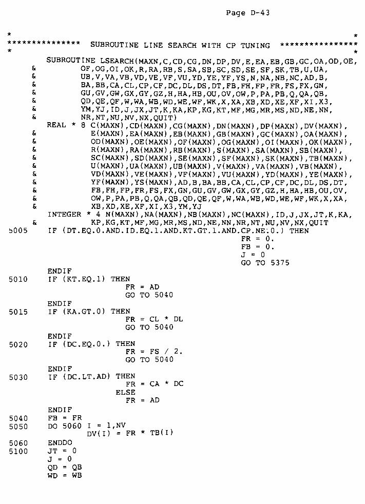
Page D-43
*
***************
*
SUBROUTINE LINE SEARCH WITH CP TUNING
Sc
Sc
Sc
Sc
Sc
Sc
Sc
Sc
Sc
&
Sc
Sc
Sc
Sc
Sc
Sc
Sc
5005
5010
5015
5020
5030
5040
5050
5060
5100
****************
*
SUBROUTINE LSEARCH (MAXN, C , CD,CG , DN, DP , DV, E, EA, EB ,GB,GC,OA,OD,OE,
OF, OG , OI , OK , R , RA , RB , S , SA ,
SB, SC , SD , SE ,
SF , SK ,TB , U ,
UA ,
UB, V , VA , VB , VD , VE , VF , VU ,
YD, YE ,
YF, YS ,
N, NA ,
NB, NC ,
AD ,B ,
BA , BB , CA , CL , CP , CF , DC ,DL
, DS , DT ,FB
, FH , FP , FR , FS , FX ,GN
,
GU,GV,GW,GX,GY,GZ,H,HA,HB,OU,OV,OW,P,PA,PB,Q,QA,QB,QD
, QE , QF , W , WA,WB
,WD ,WE ,WF,WK
,X, XA ,
XB,XD
,XE
,XF ,
X I , X 3 ,
YM,YJ,ID,J,JX,JT,K,KA,KP,KG,KT,MF,MG,MR,MS,ND,NE,NN,NR
, NT , NU ,NV
,NX
, QU I T )REAL * 8 C(MAXN) ,CD(MAXN) ,CG(MAXN) ,DN(MAXN) ,DP(MAXN) ,DV(MAXN) ,
E(MAXN) ,EA(MAXN) ,EB(MAXN) ,GB(MAXN) ,GC(MAXN) ,OA(MAXN) ,
OD(MAXN) ,OE(MAXN) ,OF(MAXN) ,OG(MAXN) ,01 (MAXN) ,OK(MAXN) ,
R(MAXN) ,RA(MAXN) ,RB(MAXN) ,S(MAXN) , SA(MAXN) ,SB (MAXN) ,SC(MAXN) ,SD(MAXN) ,SE(MAXN) ,SF(MAXN) ,SK(MAXN) ,TB(MAXN) ,
U(MAXN) ,UA(MAXN) ,UB(MAXN) ,V(MAXN) ,VA(MAXN) ,VB(MAXN) ,
VD(MAXN) ,VE(MAXN) ,VF(MAXN) ,VU(MAXN) ,YD(MAXN) ,YE(MAXN) ,
YF(MAXN) ,YS(MAXN) , AD, B , BA,BB, CA,CL,CP,CF , DC, DL,DS , DT ,
FB,FH
,FP
,FR
, FS ,FX
,GN
, GU ,GV , GW ,
GX,GY
,GZ
,H,HA
,HB
, OU ,OV
,
OW ,P, PA ,
PB, Q , QA ,
QB,QD
, QE , QF , W , WA,WB
,WD
, WE ,WF
,WK
,X,XA
,
XB , XD ,XE
, XF , X I , X 3 ,YM
, YJ
INTEGER * 4 N(MAXN) , NA(MAXN) ,NB (MAXN) ,NC(MAXN) , ID, J , JX, JT ,K,KA,
KP, KG , KT , MF
, MG ,MR
, MS ,ND
,NE
,NN
,NR
, NT , NU ,NV
,NX
, QU I T
IF (DT.EQ.0.AND. ID. EQ.l. AND. KT.GT. LAND.CP.NE.0. ) THEN
FR = 0.
FB = 0.
J = 0
GO TO 5375
ENDIF
IF (KT.EQ.l) THEN
FR = AD
GO TO 5040
ENDIF
IF (KA.GT.0) THEN
FR = CL * DL
GO TO 5040
ENDIF
IF (DC.EQ.0.) THEN
FR = FS / 2.
GO TO 5040
ENDIF
IF (DC.LT.AD) THEN
FR = CA * DC
ELSE
FR = AD
ENDIF
FB = FR
DO 5060
ENDDO
JT = 0
J = 0
QD = QB
WD = WB
I = 1,NV
DV(I) = FR * TB(I
Page D-44
5140
XD = XB
DO 5145 I = 1,NV
YD(I) = 0.0E0
VD(I) = VB(I)514 5 ENDDO
IF (MS.EQ.O) THEN
GO TO 5150ENDIF
DO 5148 IS = 1,MS
OG(IS) = SK(IS)OD(IS) = OK(IS)SD(IS) = SK(IS)
5148 ENDDO
5150 QF = QE
WF = WE
XF = XE
DO 5151 I = 1,NV
YF(I) = YE(I)
VF(I) = VE(I)5151 ENDDO
IF (MS.EQ.O) THEN
GO TO 5195
ENDIF
5180 DO 5183 IS = l.MS
OF(IS) = OE(IS)
SF(IS) = SE(IS)5183 ENDDO
5195 QE = QD
WE = WD
XE = XD
5198 DO 5201 I = 1,NV
YE(I) = YD(I)
VE(I) = VD(I)
5201 ENDDO
5202 IF (MS.EQ.O) THEN
GO TO 5225
ENDIF
5210 DO 5213 IS = 1,MS
OE(IS) = OD( IS)
SE(IS) = SD(IS)
5213 ENDDO
5225 JT = JT + 1
5226 J = J + 1
5240 DO 5244 I = 1,NV
YD ( I ) = YE ( I ) + DV ( I )
VD(I) = VB(I) + YD( I)
V(I) = VD(I)
5244 ENDDO
5245 IF (MS.EQ.O) THEN
GO TO 5270
ENDIF
5255 DO 5258 IS = 1,MS
OD(IS) = OG(IS)
OI(IS) = OD(IS)
5258 ENDDO
Page D-45
5270 CALL ANALYSIS(MAXN,C,CG,E,OI ,R,S ,U,V,B,CP, FP,H&
,P,Q,X,XI,X3,W,N,KG,NE,NR,NU)
5271 IF (MS.EQ.O) THEN
GO TO 5300
ENDIF
5285 DO 5288 IS = 1,MS
SD(IS) = S(IS)
OG(IS) = SD(IS)
5288 ENDDO
5300 MF = MF + 1
QD = QWD = W
XD = X
5315 IF (CP.EQ.0.AND.WD.GE.WE.AND.WD.GT.0. ) THEN
GO TO 5945
ENDIF
NN = 0
5345 IF (J.GE.2) THEN
GO TO 5420
ENDIF
5360 IF (XD.LE.XE) THEN
MC = 1
GO TO 5150
ENDIF
5375 GZ = FX * CF
5376 IF (FR.GT.GZ) THEN
GO TO 5405
ENDIF
5377 DO 5380 I = 1,NV
VA(I) = VD(I)
V(I) = VA(I)
5380 ENDDO
5381 IF (MS.EQ.O) THEN
GO TO 5555
ENDIF
5390 DO 5393 IS = 1,MS
OA(IS) = OD(IS)
OI(IS) = OA(IS)
5393 ENDDO
5394 GO TO 5555
5405 J = 0
5406 FR = CF * FR
5407 DO 5409 I = 1,NV
DV(I) = CF * DV(I)
5409 ENDDO
5410 GO TO 5225
5420 IF (XD.LT.XE) THEN
GO TO 5855
ENDIF
54 35 GX = XD + XF - 2.0 * XE
5436 IF (GX.EQ.0) THEN
DS = FR
ELSE
DS = FR* (XD - XE) / GX
ENDIF
Page D-46
5465 XI = 0.0E0
5466 DO 5468 I = 1,NV
XI = XI + YD(I) *YD(I)
5468 ENDDO
5469 X3=SQRT(XI)5470 YJ = X3
5471 YM = YJ -
FR / 2.0 - DS
5480 IF (YM.LT.0.0E0) THEN
WRITEU,*) 'FAILED
GO TO 5795
ENDIF
5495 DO 5499 I = 1,NV
YS(I) = YM *TB(I)
VA(I) = VB(I) + YS(I)
V(I) = VA(I)
5499 ENDDO
5500 GN = DS + FR / 2.0
5501 GU = FR * FR
5502 GV = 2.0 * FR
5510 IF (MS.EQ.O) THEN
GO TO 5555
ENDIF
5525 DO 5545 IS = 1,MS
OU = OD(IS)
OV = OE(IS)
OW = OF ( I S )
GW = OV - OU
GX = OW - OU
GY = (4.0 * GW -
GX) / GV
GX = (GW - GY *FR) / GU
GW = GN * (GX * GN + GY)
GZ = GW + OU
TEST AT 5480
OI(IS) = GZ
5 545 ENDDO
5555 CALL ANALYSIS(MAXN,C,CG, E,OI , R, S ,U, V, B ,CP , FP,H
Sc ,P,Q,X,XI ,X3,W,N,KG,NE,NR,NU)
5585 MF = MF + 1
5586 QA = Q
5587 BA = B
5588 HA = H
5589 WA = W
5590 PA = P
5591 XA = X
5600 IF (NU.GT.0) THEN
DO 5603 IU = 1,NU
UA(IU) = U(IU)
5603 ENDDO
ENDIF
5615 IF (MS.EQ.O) THEN
GO TO 5645
ENDIF
5630 DO 5637 IS = 1,MS
OA(IS) = OI(IS)
SA(IS) = S(IS)
5637 ENDDO
Page D-47
5645 IF (NE.GT.O) THEN
DO 5651 IE = 1,NE
EA(IE) = E(IE)5651 ENDDO
ENDIF
5660 IF (NR.GT.O) THEN
DO 5666 IR = 1,NR
RA(IR) = R(IR)5666 ENDDO
ENDIF
5675 IF (KG.GT.O) THEN
DO 5681 JG = 1,KG
NA(JG) = N(JG)
5681 ENDDO
ENDIF
5690 IF (XA.GT.XB) THEN
GO TO 5720
ENDIF
5705 RETURN
5720 WRITE(4,*)'
FAILED FUNCTION DECREASE TEST AT5690'
5735 GZ = FX * CF
5738 IF (FR.GT.GZ) THEN
WRITE(4,*) 'WENT TO 5825 AND5405'
GO TO 5825
ELSE
RETURN
ENDIF
5765 GZ = FX * CF
5768 IF (FR.GT.GZ) THEN
WRITEU,*) 'WENT TO 5823 FROM5765'
GO TO 5825
ENDIF
5780 IF (ABS (YM).GT.GZ) THEN
WRITEU,*) 'WENT TO 5825 FROM5780'
GO TO 58 2 5
ENDIF
5795 DO 5805 I = 1,NV
VA(I) = VB(I)
V(I) = VA(I)
5805 ENDDO
5807 IF (MS.EQ.O) THEN
GO TO 5555
ENDIF
5810 DO 5819 IS = 1,MS
OA(IS) = OK(IS)
OI(IS) = OA(IS)
5819 ENDDO
5820 GO TO 5555
5825 QE = QF
WE = WF
XE = XF
5828 DO 5831 I = 1,NV
YE(I) = YF(I)
VE(I) = VF(I)
58 31 ENDDO
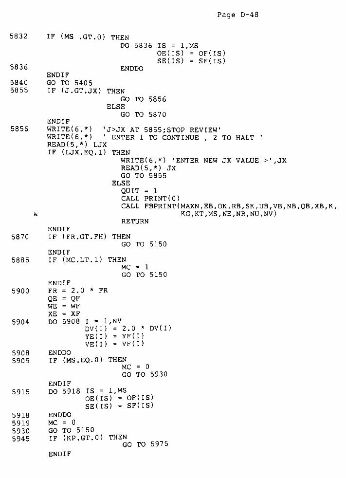
Page D-48
5832 IF (MS.GT.O) THEN
DO 5836 IS = 1,MS
OE(IS) = OF(IS)
SE(IS) = SF(IS)5836 ENDDO
ENDIF
5840 GO TO 5405
5855 IF (J.GT.JX) THEN
GO TO 5856
ELSE
GO TO 5870
ENDIF
5856 WRITE(6,*) 'J>JX AT 5855;STOPREVIEW'
WRITE (6,*)'
ENTER 1 TO CONTINUE,
2 TO HALT'
READ (5,*) LJX
IF (LJX.EQ.l) THEN
WRITEU, *) 'ENTER NEW JX VALUE >',JX
READ (5,*) JX
GO TO 5855
ELSE
QUIT = 1
CALL PRINT(O)
CALL FBPRI NT ( MAXN,EB
,OK
,RB
,SK
, UB ,VB ,
NB,QB
,XB
,K,
Sc KG,KT,MS,NE,NR,NU,NV)
RETURN
ENDIF
5870 IF (FR.GT.FH) THEN
GO TO 5150
ENDIF
5885 IF (MC.LT.l) THEN
MC = 1
GO TO 5150
ENDIF
5900 FR = 2.0 * FR
QE = QF
WE = WF
XE = XF
5904 DO 5908 I = 1,NV
DV ( I ) = 2.0 * DV ( I )
YE(I) = YF(I)
VE(I) = VF(I)
5908 ENDDO
5909 IF (MS.EQ.O) THEN
MC = 0
GO TO 5930
ENDIF
5915 DO 5918 IS = 1,MS
OE(IS) = OF(IS)
SE(IS) = SF(IS)
5918 ENDDO
5919 MC = 0
5930 GO TO 5150
5945 IF (KP.GT.0) THEN
GO TO 5975
ENDIF

Page D-49
5960 IF (QD.GT.QE) THEN
NN = 0
WRITEU, 5965)
GO TO 5345
ENDIF
5965 FORMATC IN PENALTY ZONE AT 5945 WITH WD > WE, BUT NO TUNE SINCE
ScQD > QE'
)5975 IF (NN.EQ.O) THEN
GO TO 6035
ENDIF*
*
********************* AT FIRST proBE EDGE OF PENALTY ZONE ************
* *
5990 IF (KP.EQ.O) THEN
KP = 1
GO TO 5150
ELSE
KP = 2
GO TO 6095
ENDIF
* *
******************* Qp CALCULATION ******************************
* SEGMENT 6052: FOR CP SELF-TUNING PROCESS *
* *
6035 WRITE (4,*) 'START SEGMENT 6035-'
WRITEU,*)'
AT EDGE OF PENALTY ZONE WITH WD>WE ANDQD<QE'
DO 6052 I = l.NV
VB ( I ) = VE ( I )
6052 ENDDO
6053 IF (MS.EQ.O) THEN
GO TO 6080
ENDIF
6065 DO 6067 IS = 1,MS
OK(IS) = OE(IS)
6067 ENDDO
6080 CALL NEWBP(MAXN,C,CG,E,EB,OI , OK ,R,RB
, S , SK,U , UB, V, VB ,B
, BB,
Sc CP ,FP ,
H,HB ,
P,PB , Q ,
QB, W ,
WB,X,X I
,X 3
,XB
,N
, NB , KG , MS
Sc , NU ,NE
,NR
,NV )
6081 NT = ND
6082 ND = 1
6083 CALL SDIR(MAXN,C,CD,CG,DN,DP, E,GB,GC,OI ,R, S, SB, SC, SK,TB, U,
t V ,VU ,
VB,N,NB
,NC ,
B,CP , DC ,
DT,FP
,GX
, GY ,H,P, Q ,
X, XI ,
Sc X 3 ,W
,WK ,
I D ,KA
,KG , MG ,
MR , MS ,ND
, NE , NR ,NX
, NU , NV . QU I T )
IF (QUIT.EQ.l) THEN
RETURN
ENDIF
6084 FB = FR
6085 NN = 1
6086 KP = 0
6087 ND = NT
6088 GO TO 5050
6095 WRITEU,*) 'FOR CP CALCULATION AT6095'
6110 IF (WD.NE.WF) THEN
CP =.75
* (QF - QD) / (WD -
WF)
ENDIF
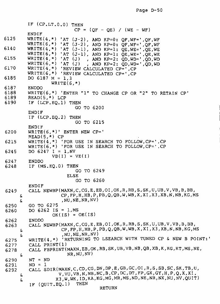
Page D-50
IF (CP.LT.O.O) THEN
CP = (QF - QE) / (WE -
WF)ENDIF
6125 WRITEU,*) 'AT (J-2), ANDKP=0: QF,WF= ',QF,WF
WRITE(6,*) 'AT (J-2), ANDKP=0: QF,WF= '
,QF,WF
6140 WRITEU,*) 'AT (j-1) , ANDKP=1: QE,WE= '
,QE,WE
WRITEU, *) 'AT (J-1), AND KP=1: QE,WE= ',QE,WE
6155 WRITEU.-*) 'AT (J) , ANDKP=2: QD,WD= '
,QD,WD
WRITEU, *) 'AT (J) , AND KP=2: QD,WD= ',QD,WD
6170 WRITEU,*) 'REVIEW CALCULATED CP= '
,CP
WRITEU,*) 'REVIEW CALCULATED CP=',CP
6185 DO 6187 M = 1,3
WRITEU,*)
6187 ENDDO
6188 WRITE (6,*) 'ENTER"1"
TO CHANGE CP OR"2"
TO RETAINCP'
6189 READ(5,*) LCP
6190 IF (LCP.EQ.l) THEN
GO TO 6200
ENDIF
IF (LCP.EQ.2) THEN
GO TO 6215
ENDIF
6200WRITEU,*)'
ENTER NEW CP= '
READ(5,*) CP .
6215 WRITEU,*) 'FOR USE IN SEARCH TO FOLLOW, CP= ', CP
WRITEU,*) 'FOR USE IN SEARCH TO FOLLOW, CP='
,CP
6245 DO 6247 I = 1,NV
VB(I) = VE(I)
6247 ENDDO
6248 IF (MS.EQ.O) THEN
GO TO 6249
ELSE
GO TO 6260
ENDIF
6249 CALL NEWBP(MAXN,C,CG,E,EB,OI ,OK,R, RB , S,SK,U,UB, V, VB ,B
,BB ,
S. CP ,FP ,
H,HB
,P ,
PB, Q ,
QB,W,WB
,X,X I , X3 ,
XB,N
,NB
, KG , MS
Sc ,NU ,
NE,NR ,
NV )
6250 GO TO 6275
6260 DO 6262 IS = l.MS
OK(IS) = OE(IS)
6262 ENDDO
6263 CALL NEWBP(MAXN,C,CG,E, EB,OI ,OK,R,RB, S,SK, U,UB, V,VB,B, BB ,
Sc CP,FP,H,HB,P,PB,Q,QB,W,WB,X,XI,X3,XB,N,NB,KG,MS
& ,NU,NE,NR,NV)
6275 WRITEU,*) 'RETURNING TO LSEARCH WITH TUNED CP Sc NEW B POINT:
6277 CALL PRINT(l)
6278 CALL FBPRINT (MAXN,EB ,
OK,RB ,
SK ,UB ,
VB,NB
,QB
,XB
,K, KG , KT , MS ,
NE,
& NR,NU,NV)
6290 NT = ND
6291 ND = 1
6292 CALL SDIR(MAXN,C,CD,CG, DN, DP, E,GB,GC,OI ,R, S , SB,SC,SK,TB,U,
& V,VU,VB,N,NB,NC,B,CP,DC,DT,FP,GX,GY,H,P,Q,X,XI,
ScX3,W,WK,ID,KA,KG,MG,MR,MS,ND,NE,NR,NX,NU,NV,QUIT)
IF (QUIT.EQ.l) THEN
RETURN
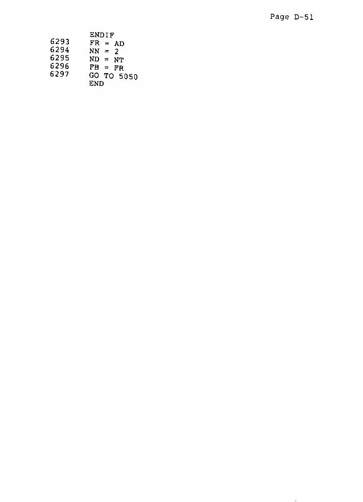
Page D-51
ENDIF
6293 FR = AD
6294 NN = 26295 ND = NT
6296 FB = FR6297 GO TO 5050
END
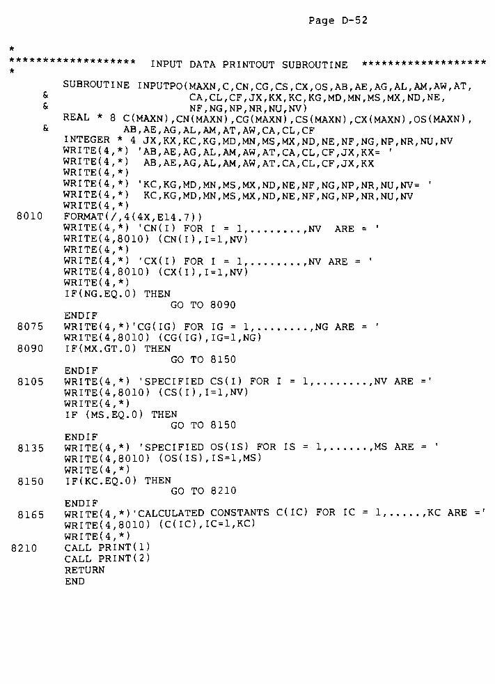
Page D-52
*
*******************INPUT DATA PRINTOUT SUBROUTINE
*******************
*
SUBROUTINE INPUTPO(MAXN,C,CN,CG, CS ,CX,OS , AB, AE , AG, AL, AM, AW, AT,& CA
, CL ,CF
,JX
, KX , KC , KG ,MD
,MN
, MS ,MX
,ND ,
NE ,
& NF,NG,NP,NR,NU,NV)REAL * 8 C(MAXN) ,CN(MAXN) ,CG(MAXN) ,CS(MAXN) ,CX(MAXN) ,OS(MAXN) ,
& AB,AE,AG,AL,AM,AT,AW,CA,CL,CFINTEGER * 4 JX,KX,KC,KG,MD,MN,MS,MX,ND,NE,NF,NG,NP,NR,NU,NV
WRITE(4,*) 'AB,AE,AG,AL,AM,AW,AT,CA,CL,CF,JX,KX= '
WRITE (4,*) AB,AE,AG,AL,AM,AW,AT,CA,CL,CF,JX,KX
WRITE(4,*)
WRITE(4,*) 'KC,KG,MD,MN,MS,MX,ND,NE,NF,NG,NP,NR,NU,NV= '
WRI TE ( 4 ,
* ) KC , KG , MD, MN
, MS , MX,ND
, NE , NF ,NG , NP , NR , NU ,
NV
WRITE(4,*)
8010 FORMAT(/,4(4X,E14.7) )WRITE (4..*) 'CN(I) FOR I = 1, ,NV ARE =
'
WRITEU, 8010) (CN(I) ,I = 1,NV)WRITEU,*)
WRITE (4,*) "CX(I) FOR I = 1, ,NV ARE =*
WRITEU, 8010) (CX(I) ,I = 1,NV)
WRITEU,*)
IF(NG.EQ.O) THEN
GO TO 8090
ENDTF
8075 WRITEU,*) 'CG(IG) FOR IG = 1, ,NG ARE ='
WRITEU, 8010) (CG(IG) ,IG=1,NG)
8090 IF(MX.GT.O) THEN
GO TO 8150
ENDIF
8105 WRITEU,*) 'SPECIFIED CS ( I ) FOR I = 1, ,NV ARE='
WRITEU, 8010) (CS(I) ,I = 1,NV)
WRITEU,*)
IF (MS.EQ.O) THEN
GO TO 8150
ENDIF
8135 WRITEU,*) 'SPECIFIED OS(IS) FOR IS = 1, ,MS ARE ='
WRITEU, 8010) (OS(IS) ,IS = 1,MS)
WRITEU,*)
8150 IF(KC.EQ.O) THEN
GO TO 8 210
ENDIF
8165 WRITEU,*) 'CALCULATED CONSTANTS C(IC) FOR IC = 1, ,KC ARE='
WRITEU, 8010) (C(IC),IC=1,KC)
WRITEU,*)
8210 CALL PRINT(l)
CALL PRINT(2)
RETURN
END

Page D-53
*
***** MINIMAL BASEPOINT PRINTOUT SUBROUTINE (OPTION ,NP = 1)
*******
*
SUBROUTINE MBPRINT(VB,QB,XB, KT)REAL * 8 VB,QB,XB
INTEGER * 4 KT
WRITE (4, 10) KT,VB,XB,QB
10 FORMAT('
KT,VB(1) ,XB,QB ='
, 1 3 , 3X, 3 (E14 . 7 , 3X) , /)
CALL PRINT(l)
CALL PRINT(2)
RETURN
END************************************************************************
*
**** FULL BASEPOINT PRINTOUT (OPTION,
NP = 2) SUBROUTINE*************
*
SUBROUTINE FBPRINT (MAXN, EB , OK,RB,SK,UB, VB,NB,QB, XB,K,KG,KT,MS ,NE
S< ,NR,NU,NV)
REAL * 8 EB(MAXN),OK(MAXN),RB(MAXN),SK(MAXN),UB(MAXN),VB(MAXN),
Sc QB,XB
INTEGER * 4 NB(MAXN) ,K ,KT,KG,MS ,NE ,NR,NU,NV
WRITE (4, 10) KT,K,XB,QB
10 FORMATC KT,K,XB,QB =*
,2 ( I 5 ) , 5X, 2 ( E14 . 7 , 3X) , /)
WRITE (4.*) 'VB(I) FOR I = 1, ,NV=
'
WRITEU, 20) (VB(I) ,I = 1,NV)
20 FORMAT (/, 4 ( 4X, E14.7) )
WRITE(4,*)
IF(MS.EQ.O) THEN
GO TO 30
ENDIF
WRITE (4,*)'
OK (IS) FOR IS = 1, ,MS ARE =
'
WRITEU, 20) (OK(IS) ,IS = 1,MS)
WRITE (4,*)
WRITEU,*) 'SK(IS) FOR IS = 1, ,MS ARE =
'
WRITEU,*) (SK(IS),IS=1,MS)
WRITEU,*)
30 IF (NU.LE.0) THEN
GO TO 40
ENDIF
WRITE (4,*) 'UB(IU) FOR IU = 1, ,NU ARE =
WRITEU, 20) (UB(IU),IU=1,NU)
WRITEU,*)
40 IF (NE.LE.0) THEN
GO TO 4 5
FNDI F
WRITEU,*) 'EB(IE) FOR IE = 1, ,NE ARE =
'
WRITEU, 20)(EB(IE),IE=1,NE)
WRITEU,*)
45 IF(NR.LE.O) THEN
GO TO 60
ENDIF .
.Tr, ._.
WRITEU,*) 'RB(IR) FOR IR = 1 ,NR ARE =
WRITEU, 20)(RB(IR),IR=1,NR)
WRITEU,*)
60 IF (KG.LE.0) THEN
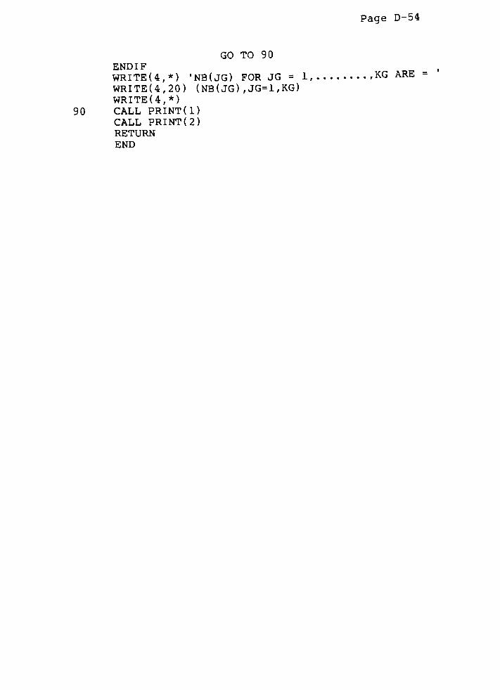
Page D-54
GO TO 90
ENDIF
WRITEU,*) 'NB(JG) FOR JG = 1, ,KGARE _
WRITE(4,20) (NB(JG) ,JG=1,KG)
WRITE(4,*)
90 CALL PRINT(l)
CALL PRINT(2)
RETURN
END

Page D-55
************************************************************************
*SUB FUNCTIONS
*
************************************************************************
* *
*******************SIGN SUB-FUNCTION
********************************
* *
FUNCTION SGN(P)REAL * 8 SGN,P
IF (P.GT.O) THEN
SGN = 1
ENDIF
IF (P.EQ.O) THEN
SGN = 0
ENDIF
IF (P.LT.O) THEN
SGN =-1
ENDIF
RETURN
END
************************************************************************
* *
**************** RANDOM NUMBER GENERATION SUB-FUNCTION ****************
* *
FUNCTION RND(SEED)
REAL * 8 RND, PI, FRAC, SEED
PI = 4.0*ATAN(1.0)
BASE = (PI + SEED)**5
FRAC = I FIX (BASE)
RND = BASE - FRAC
RETURN
END
Page D-56
*
****
*
*
*
*
*
*
*
*
* * * *
*
*
*
*
*
*
*
*
*
*
*
*
*
*
*
*
*
*
*
*
*
*
*
*
*
*
*
*
*
*
*
*
*
*
*
*
*
*
*
*
*
*
*
*
THIS SUBROUTINE CALCULATES THE VALUE OF THE OBJECTIVE FUNC
TION, Q, REGIONAL CONSTRAINTS, R, AND EQUALITY CONSTRAINTS, E
FOR A GIVEN BASEPOINT MATRIX, V. THE FOLLOWING ANALYSIS IS
FOR THE BALANCING OF AN INLINE FOUR BAR MECHANISM.
ANALYSIS WRITTEN BY; TIMOTHY C. HEWITT,
AUGUST 1984
******************VARIABLE IDENTIFICATION
AOiD
AOiDMAX
AP
AOiDRMS
AU
C
CP
CG
CG(1)
CG(2)
CG(3)
CGU)
CG(5)
CGU)
CG(7)
CGU)
CGU)
CG(10)
CG(ll)
CG(12)
CG(13)
CG(14)
CG(15)
CG(16)
CG(17)
CG(18)
CG(19)
CG(20)
CG(21)
CG(22)
CG(23)
CG(24)
CG(25)
CG(26)
CG(27)
CG(28)
CG(29)
CTHTT
DS1
DS2
***********************
*
TIME DERIVATIVE OF THE TOTAL ANGULAR MOMENTUM OF *
THE MECHANISM WITH RESPECT TO THE JOINT Oi .
*
THE MAXIMUM AOiD IN ONE REVOLUTION OF THE INPUT LINK.*
VALUE OF PI (3.14159) .
*
RMS VALUE OF AOiD.*
DIFFERENCE IN THE LIMITS OF INTEGRATION.*
MATRIX OF CALCULATED CONSTANTS (NOT USED).*
PENALTY FUNCTION TUNING PARAMETER.*
MATRIX OF GIVEN CONSTANTS.*
LENGTH OF LINK 1 ( IN) .
*
NORMALIZED LENGTH OF LINK 2. *
II tl If If n *
ir it if it
^ ^
*
ANGULAR VELOCITY OF THE INPUT LINK (RAD/S). *
ACCELERATION OF THE INPUT LINK (RAD/S/S). *
GROUND BEARING FORCE WEIGHTING FACTOR IN Q .
INPUT TORQUE WEIGHTING FACTOR IN Q.
DISTANCE FROM JOINT03'
TO EXTERNAL LOADING POINT
APPLICATION ON LINK 3.
DISTANCE FROM JOINT 01 TO REAL LINK
MASS
MASS
II II
02II II 03'
OF REAL LINK 1 (LB)If Tl II
2 (LB)IT If II
3 (LB)
MOMENT OF INERTIA C
1
2
3
C.G.
C.G.
C.G.
LOC
LOC
LOC
(IN)
(IN)
(IN)
THE REAL LINK 1 (IB-IN2)
ANGLE FROM LINE 01 '02 TO REAL LINK 1 C.G.ii
o2 04" " "
2"
H " "
03'
04" " "
3"
DENSITY OF THE COUNTERWEIGHTS ADDED
THICKNESS OF THE COUNTERWEIGHTS ADDED
MAXIMUM COUNTERWEIGHT ANGLE (I.E. 2*PI)
MAXIMUM C.W. RADIUS (IN).
MAXIMUM ALLOWABLE NORMALIZED
LOC,
(LB/IN3)
(IN).
RMSit
SHAKING
BEARING
SHAKING
FORCE .
FORCE .
MOMENT ,
COSINE OF THTT.
BODY COORDINATES FOR THE'
CENTER OF GRAVITY FOR THE
BODY COORDINATES FOR THE'
"
INPUT TORQUE.
x"
LOCATION OF THE
iTH LINK (IN) .
y"
LOCATION OF THE
*
*
*
*
*
*
(RAD)it *
" *
*
*
*
*
*
*
*
*
*
COMBINED*
*
COMBINED*
Page D-57
*
*
*
*
*
*
*
*
*
*
*
*
*
*
*
*
*
*
*
*
*
*
*
*
*
*
*
*
*
*
*
*
*
*
*
*
*
*
*
*
*
*
*
*
*
*
*
*
*
*
*
*
*
*
*
E
F
FP
FijFijX
FijY
FijMAX
FijRMS
FSH
FSHMAX
FSHRMS
FX
FY
G
IC
II
IT
Ll
L2
LC
LT
MI
Ml
M2
MC
MT
N
NC
NGQNE
NR
NRMS
NU
01
P
PI
QR
RMAXB
RMAXH
S
STHTT
SUM
SUMAOiD
SUMF i jSUMFSH
SUMTD
TD
CENTER OF GRAVITY FOR THE iTH LINK (IN).
MATRIX OF EQUALITY CONSTRAINTS (NOT USED).
DERIVATIVE OF THE OPTIMIZATION QUANTITY W.R.T. THT1.
PENALTY FUNCTION FACTOR.
THE NORMALIZED BEARING FORCE BETWEEN LINKS i AND j."X"
COMPONET OF THE FORCE Fij."Y"
COMPONET OF THE FORCE Fij.
MAXIMUM Fij FORCE .
RMS Fij.
NORMALIZED SHAKING FORCE OF THE MECHANISM.
MAXIMUM FSH
RMS FSH
EXTERNAL X-FORCE APPLIED TO THE OUTPUT LINK (LINK 3).n V_ " " " " " " " "
ABS ICCA OF THE SAMPLING POINT; USED IN GAUSSIAN
QUADRATURE INTEGRATION.
MASS MOMENT OF INERTIA OF THE iTH COUNTERWEIGHT
ABOUT ITS C.G. (LB-IN2) .
NORMALIZED MASS MOMENTS OF INERTIA MATRIX WHERE EACH.
INERTIA IS ABOUT THE iTH JOINT.
MASS MOMENT OF INERTIA OF THE iTH COUNTERWEIGHT AND
AND iTH REAL LINK ABOUT THEIR COMBINED C.G. ( LB-IN2 ) .
DIST. OF TWO POINT MASS MODEL TO MASS M1(IN)."
M2(IN).
RADIUS OF THE iTH COUNTERWEIGHT (IN) .
LENGTH FROM iTH JOINT TO THE COMBINED C.G. LOC. (IN).
NORMALIZED MASS MATRIX FOR THE TWO POINT MASS MODEL
FOR THE iTH LINK.
MASS IN THE Ll DIR. FOR THE iTH LINK(LB).
L2" " " " "
(LB).
MASS OF THE iTH COUNTERWEIGHT ( LB ) .
"
COMBINED LINK(LB).
NOT USED.
NUMBER OF COUNTERWEIGHTS TO BE ADDED ( 1 < NC < 3 ) .
NUMBER OF SAMPLING POINTS FOR NUMERICAL INTEGRATION."
EQUALITY CONSTRAINTS.
NUMBER OF REGIONAL CONSTRAINTS.
DETERMINES THE TYPE OF INTEGRATION USED.
NUMBER OF VARIABLES IN MATRIX U (NOT USED).
NOT USED.
PENALTY FUNCTION.
NORMALZED MASS DISTANCE PRODUCT OF THE TWO POINT
MODEL.
OBJECTIVE FUNCTION.
REGIONAL CONSTRAINT MATRIX.
*
*
*
*
*
*
*
*
*
*
*
*
*
*
*
*
*
*
*
*
*
*
*
*
*
*
*
*
MASS*
*
*
THE
THE
NOT
SIN
SUM
SUM
SUM
SUM
SUM
MAXIMUM
MAXIMUM
USED.
OF THTT."
F" '
S
AO i D'
S
Fij 'S
FSH'S
TD'S
RMS
RMS
BEARING
SHAKING
FORCE .
MOMENT ,
OF
OF
OF
OF
OF
USED TO CALCULATE AOiDRMS.
F i j RMS .
FSHRMS.
TDRMS.
*
*
*
NORMALIZED DRIVING (INPUT) TORQUE,
Page D-58
*TE
*TED
*TH
*THTi
*THTC
*THTT
*
*Tl
*TJ
*TK
*TKD
* TL
* TN
*
* TT* U* V
*
* X
* zz
*
*
ANGULAR VELOCITY RATIO OF LINK 3 TO LINK 1.
TIME DERIVATIVE OF"
TE ".
NORMALIZED ANGULAR ACCELERATION OF LINK 2.
THE ANGLE BETWEEN LINK i AND THE FIXED X-AXIS .
" " " " " " "iTH COUNTERWEIGHT .
ANGLE BETWEEN THE FIXED X-AXIS AND THE COMBINED C.G.
LOCATION FOR THE iTH LINK.
NORMALIZED ANGULAR ACCELERATION OF LINK 3.ti tt n n ri -j
ANGUALR VELOCITY RATIO OF LINK 2 TO LINK 1.
TIME DERIVATIVE OF TK.
NORMALIZED EXTERNAL LOADING TORQUE.
BETA, ANGLE BETWEEN FIXED X-AXIS AND EXTERNAL
LOADING POINT APPLICATION ON LINK # 3 .
NORMALIZED GENERAL EXTERNAL FORCE.
NOT USED.
SCALED VARIABLES ; ANGLES AND RADII OF THE
COUNTERWEIGHTS.
PENALIZED OPTIMIZATION QUANTITY.
WEIGHTING COEFFICIENTS FOR GAUSSIAN QUADRATURE
INTEGRATION.
*
*
*
*
*
*
*
*
*
*
*
*
*
*
*
*
*
*
*
*
*
*
MAIN SUB- PROGRAM ****************************
*
***********************
*
SUBROUTINE ANALYS IS ( MAXN, C , CG ,
E,OI
,R, S ,'U ,
V,B
,CP
,FP
,H
Sc ,P,Q,X,XI ,X3,W,N,KG,NE,NR,NU)
REAL * 8 C(MAXN) ,CG(MAXN) ,E(MAXN) ,G(24) ,0I(MAXN) ,11(10) ,
MI (10), PI (10) ,R(MAXN) ,RR(19) ,S(MAXN) ,U(MAXN) ,V(MAXN) ,
ZZ ( 2 4 ) ,A
,AOID
,AOIDMX
, AOIDRS ,A03D
,A03DMX
, A03DRS ,AP
, AU ,
AV,AX
,B
,BR
,CA
,CP ,
CTHTT,DEN
, DS 1 ,DS2
,F, F2 1
,F2 IX
,F2 1Y
,
F21MAX,F21RMS,F32,F32X,F32Y,F32MAX,F32RMS,F41,F41X,
F4 1Y,F4 1MAX
,F4 1RMS ,
F4 3 ,F4 3X
,F4 3Y , F4 3MAX
,F4 3RMS ,
FP,FSH
,
FSHMAX,FSHRMS ,
FX,FY
,H,I C ,
IT, LC ,
LT,L 1
,L2
,Ml
,M2
,MC ,
MT,P
,
Q ,RMAXB
,RMAXH
,SUM
,SUMAOID
,SUMA03D
,SUMFSH
,SUMF2 1
, SUMF3 2,
SUMF4 1,SUMF4 3 ,
SUMTD,STHTT
,TA , TBB , TC , TD ,
TDMAX, TDRMS , TE ,
TF , TG ,TH
,THTI
,THT2 , THT3 ,
THTT, THTC , TED ,
TKD,T I
, TJ ,TK
,TL
,
TM,TN ,
TO,TP
, TQ ,TR
,TS ,
TT, TU ,
TV,TY
,TZ
,X,X I
, X3 , W
INTEGER * 4 N(MAXN) ,KG , NC, NE,NR, NU,NRMS
COMMON G ,ZZ
,RR
,AP
,FSHMAX
,F2 1MAX
,F3 2MAX
, F4 1MAX,F4 3MAX
, AOIDMX,
A03DMX, TDMAX, FSHRMS, F21RMS , F32RMS , F41RMS , F4 3RMS ,
AOIDRS ,A03DRS ,
TDRMS/Al/NRMS , NC , NGQ
= 0.0
Sc
Sc
Sc
Sc
Sc
Sc
Sc
Sc
Sc
Sc
Sc
Sc
TY
TZ
AU
IF
= 2.0*AP
= TZ - TY
( NC . EQ . 0 ) THEN
DO 3 I = 1,6
V(I) =
ENDIF
IF (NC.EQ.l)
ENDDO
THEN
V(2) =
V(3) =
V(5) =
V(6) =
.CASE OF NO COUNTERWEIGHTS
0.0
.CASE OF 1 COUNTERWEIGHT
0
0
0
0
ENDIF
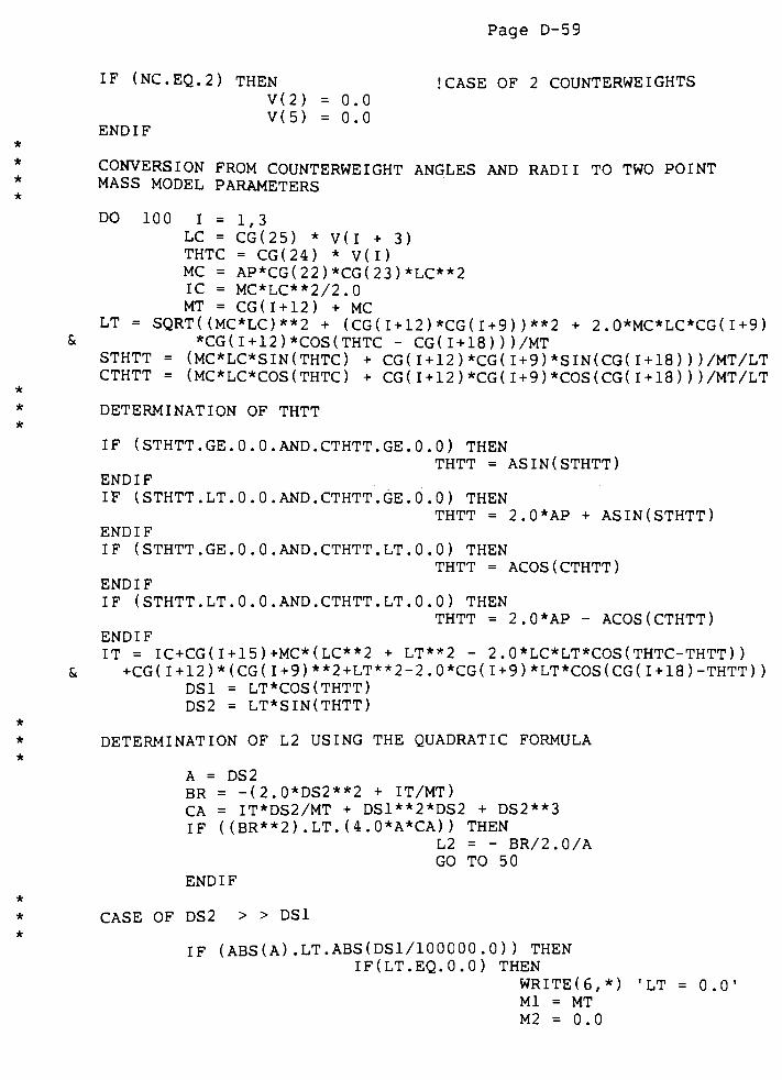
Page D-59
*
*
*
*
*
*
*
*
*
*
*
*
*
IF
ENDIF
(NC..EQ..2) THEN
V(2) = 0,.0
V(5) = 0,.0
.CASE OF 2 COUNTERWEIGHTS
CONVERSION FROM COUNTERWEIGHT ANGLES AND RADII TO TWO POINT
MASS MODEL PARAMETERS
DO 100 I =
LC =
THTC
MC =
IC =
MT =
LT
1,3
CG(25) * V(I + 3)= CG(24) *
V(I)
AP*CG(22)*CG(23)*LC**2
MC*LC**2/2.0
CG(I+12) + MC= SQRT((MC*LC)**2 + (CG( 1+12 ) *CG( 1+9 )) **2 + 2 . 0*MC*LC*CG( 1+9 )
*CG(l+12)*COS(THTC -
CG( 1+18 ) ) ) /MT
STHTT = (MC*LC*SIN(THTC) + CG( 1+12 ) *CG( 1+9 ) *SIN(CG( 1+18 ))) /MT/LT
CTHTT = (MC*LC*COS(THTC) + CG( 1+12 ) *CG( 1+9 ) *COS (CG( 1+18 ))) /MT/LT
DETERMINATION OF THTT
IF ( STHTT. GE. 0.0. AND. CTHTT. GE . 0.0) THEN
THTT = AS IN (STHTT)ENDIF
IF ( STHTT. LT. 0.0. AND. CTHTT. GE. 0.0) THEN
THTT = 2.0*AP + ASIN( STHTT)
ENDIF
IF ( STHTT. GE. 0.0. AND.CTHTT.LT. 0.0) THEN
THTT = ACOS( CTHTT)
ENDIF
IF ( STHTT. LT. 0.0. AND.CTHTT.LT. 0.0) THEN
THTT = 2.0*AP -
ACOS( CTHTT)
ENDIF
IT = IC+CG(I+15)+MC*(LC**2 + LT**2 - 2 . 0*LC*LT*COS(THTC-THTT ) )
+CG(l+12)*(CG(l+9)**2+LT**2-2.0*CG(l+9)*LT*COS(CG(l+18)-THTT) )
DS1 = LT*COS(THTT)
DS2 = LT*SIN(THTT)
DETERMINATION OF L2 USING THE QUADRATIC FORMULA
A = DS2
BR = -(2.0*DS2**2 + IT/MT)
CA = IT*DS2/MT + DS1**2*DS2 + DS2**3
IF ( (BR**2) .LT. (4.0*A*CA) ) THEN
L2 = - BR/2.0/A
GO TO 50
ENDIF
CASE OF DS2 > > DS1
IF (ABS(A) .LT.ABS(DS1/100000.0) ) THEN
IF(LT.EQ.O.O) THEN
WRITEU,*)
Ml = MT
M2 = 0.0
LT =0.0'
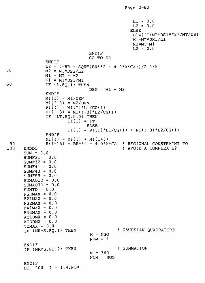
Page D-60
50
60
90
100
Ll = 0.0
L2 = 0.0
ELSE
Ll= ( IT+MT*DS1**2 ) /MT/DS1
M1=MT*DS1/L1
M2=MT-M1
L2 = 0.0
ENDIF
GO TO 60
ENDIF
L2 = (-BR + SQRT(BR**2 - 4 . 0*A*CA) ) /2 . 0/A
M2 = MT*DS2/L2
Ml = MT - M2
Ll = MT*DS1/M1
IF (I. EQ.l) THEN
DEN = Ml + M2
ENDIF
MI(I) = Ml/DEN
MI (1 + 3) = M2/DEN
PI(I) = MI(I)*L1/CG(1)
PKl + 3) = MI(I + 3)*L2/CG(1)
IF (LT.EQ.0.0) THEN
II(I) = IT
ELSE
= PI(I)*L1/CG(1)
ENDIF
MI (I) =
R(I+16) = BR**2
IKI)
MI ( I ) MI( 1 + 3)- 4.0*A*CA
0
ENDDO
SUM =
SUMF21
SUMF32
SUMF41
SUMF4 3
SUMFSH
SUMAOID
SUMA03D
+ PI(I+3)*L2/CG(1)
REGIONAL CONSTRAINT TO
AVOID A COMPLEX L2
0
0.
0.
0.
0.
0.
= 0
= 0
0
0
SUMTD =0.0
FSHMAX =0.0
F21MAX =0.0
F32MAX =0.0
F41MAX = 0.0
F43MAX =0.0
AOIDMX =0.0
A03DMX =0.0
TDMAX =0.0
IF (NRMS.EQ 1) THEN
ENDIF
IF (NRMS.EQ, 2) THEN
M = NGQ
NUM = 1
M = 360
NUM = NGQ
! GAUSSIAN QUADRATURE
! SUMMATION
ENDIF
DO 200 I = 1,M,NUM
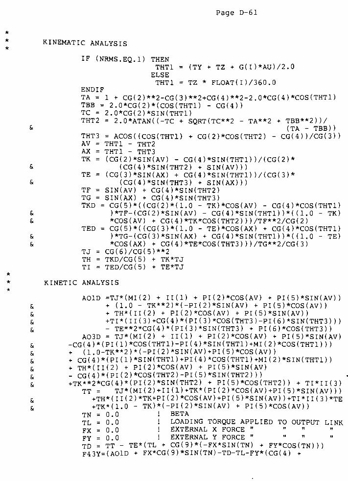
*
*
Page D-61
KINEMATIC ANALYSIS
IF (NRMS.EQ. 1) THEN
THT1 = (TY + TZ + G(l)*AU)/2.0
ELSE
THT1 = TZ * FLOAT(I)/360.0
ENDIF
TA = 1 + CG(2)**2-CG(3)**2+CG(4)**2-2.0*CG(4)*COS(THT1)
TBB = 2.0*CG(2)*(COS(THT1) -
CGU))
TC = 2.0*CG(2)*SIN(THT1)THT2 = 2.0*ATAN( (-TC + SQRT(TC**2 - TA**2 + TBB**2))/
& (TA - TBB) )
THT3 = AC0S((C0S(THT1) + CG( 2 ) *COS (THT2 ) - CG( 4 ) ) /CG( 3 ) )AV = THT1 - THT2
AX = THT1 - THT3
TK = (CG(2)*SIN(AV) -
CG( 4 ) *SIN(THT1 ) ) / (CG( 2 ) *
S< (CG(4)*SIN(THT2) + SIN(AV)))
TE = (CG(3)*SIN(AX) + CG( 4 ) *SIN(THT1 ) ) /(CG( 3 ) *
Sc (CG(4)*SIN(THT3) + SIN(AX) ) )TF = SIN(AV) + CG(4)*SIN(THT2)
TG = SIN(AX) + CG(4)*SIN(THT3)
TKD = CG(5)*( (CG(2)*(1.0 -
TK)*COS(AV)-
CG( 4 ) *COS (THT1 )Sc )*TF-(CG(2)*SIN(AV) - CG(4 ) *SIN(THT1 ) ) * ( ( 1 . 0 - TK)
Sc *COS(AV) + CG(4)*TK*COS(THT2) ) )/TF**2/CG(2)TED = CG(5)*((CG(3)*(1.0 -
TE)*COS(AX) + CG( 4 ) *COS (THT1 )Sc )*TG-(CG(3)*SIN(AX) + CG( 4 ) *SIN(THT1 ) ) * ( ( 1 . 0 -
TE)
Sc *COS(AX) + CG(4)*TE*COS(THT3) ) )/TG**2/CG(3)
TJ = CG(6)/CG(5)**2
TH = TKD/CGU) + TK*TJ
Tl = TED/CGU) + TE*TJ
KINETIC ANALYSIS
AOID =TJ*(MI(2) + 11(1) + PI(2)*C0S(AV) + PI ( 5 ) *SIN( AV) )
Sc + (1.0 -
TK**2)*(-PI(2)*SIN(AV) + PI ( 5 ) *COS ( AV) )
Sc + TH*(II(2) + PI(2)*C0S(AV) + PI ( 5 ) *SIN( AV) )
Sc +TI*( II(3)+CG(4)*(PI(3)*C0S(THT3)-PI(6)*SIN(THT3) ) )
S,- TE**2*CG(4)*(PI(3)*SIN(THT3) + PI ( 6 ) *COS (THT3 ) )
A03D = TJ*(MI(2) + 11(1) + PI(2)*C0S(AV) + PI ( 5 ) *SIN( AV)
Sc -CG(4)*(PI(1)*C0S(THT1)-PI(4)*SIN(THT1)+MI(2)*C0S(THT1) ) )
Sc + (1.0-TK**2)*(-PI(2)*SIN(AV)+PI(5)*COS(AV) )
Sc + CG(4)*(PI(1)*SIN(THT1)+PI(4)*C0S(THT1)+MI(2)*SIN(THT1) )
S, + TH*(II(2) + PI(2)*C0S(AV) + PI ( 5 ) *SIN( AV)
S.- CG(4)*(PI(2)*C0S(THT2)-PI(5)*SIN(THT2) ) )
Sc +TK**2*CG(4)*(PI(2)*SIN(THT2) + PI ( 5 ) *C0S (THT2 ) ) + TI*II(3)
TT - TJ*(MI(2)+II(1)+TK*(PI(2)*C0S(AV)+PI(5)*SIN(AV) ) )g.
+TH* (11(2) *TK+PI ( 2 ) *COS ( AV ) +P I ( 5 ) *S IN ( AV ) ) +TI * 1 1 ( 3 ) *TE
& +TK*(1.0- TK)*(-PI(2)*SIN(AV) + PI ( 5 ) *COS ( AV) )
TN = 0.0 ! BETA
TL = 0.0 ! LOADING TORQUE APPLIED TO OUTPUT LINK
FX = 0.0 ! EXTERNAL X FORCE"
FY = 0.0 ! EXTERNAL Y FORCE"
TD = TT- TE*(TL + CG( 9 ) * ( -FX*SIN(TN) + FY*COS(TN)))
F43Y=(A01D + FX*CG(9)*SIN(TN)-TD-TL-FY*(CG(4) +
it

Page D-62
&CG(9)*COS(TN)))/CG(4)
F32Y= -
F43Y - PI ( 3 ) *( -TI*C0S(THT3 ) + TE**2*SIN(THT3 ) )& -
PI(6)*(TI*SIN(THT3) + TE**2*COS(THT3 ) ) - FY
F32X= ( F32Y*CG( 3 ) *C0S(THT3 ) +TL-I I ( 3 ) *TI+FY*CG( 9 ) *COS ( TN)& -
FX*CG(9)*SIN(TN) )/(CG(3)*SIN(THT3) )F43X =
-F32X- PI ( 3 ) *(TI *SIN(THT3 ) + TE**2*COS(THT3 ) )
& + PI(6)*(-TI*C0S(THT3) + TE**2*SIN(THT3 ) ) - FX
F41Y = (-A03D+TD+TL+CG(9)*(FY*COS(TN)-FX*SIN(TN) ) )/CG(4)
F21Y =-F41Y
-
PI(1)*(-TJ*C0S(THT1) + SIN(THTl))-
& PI(4)*(TJ*SIN(THT1) +C0S(THT1))
F21X =-F32X + PI(2)*(TH*SIN(THT2) + TK**2*COS(THT2 ) )
S< + PI(5)*(TH*C0S(THT2)- TK**2*SIN(THT2 ) )S< + MI(2)*(TJ*SIN(THT1) + COS(THTl))
F41X =-F21X
-
PI(1)*(TJ*SIN(THT1) + COS(THTl)) +
& PI(4)*(-TJ*C0S(THT1) + SIN(THTl))
FSH = SQRT( (F41X+F43X+FX)**2 + ( F41Y+F43Y+FY) **2 )F21 = SQRT(F21X**2 + F21Y**2)
F32 = SQRT(F32X**2 + F32Y**2)
F41 = SQRT(F41X**2 + F41Y**2)
F43 = SQRT(F43X**2 + F43Y**2)
F = CG(7)*SQRT(F41**2 + F43**2) + CG( 8 ) *ABS(TD)IF (NRMS.EQ. 1) THEN
SUM = SUM + ZZ(I)*F
SUMFSH = SUMFSH + ZZ(l)*FSH**2
SUMF21 = SUMF21 + ZZ(I)*F21**2
SUMF32 = SUMF32 + ZZ(l)*F32**2
SUMF41 = SUMF41 + ZZ(l)*F41**2
SUMF43 = SUMF43 + ZZ(l)*F43**2
SUMAOID = SUMAOID + ZZ( I ) *A01D**2
SUMA03D = SUMA03D + ZZ( I ) *A03D**2
SUMTD = SUMTD + ZZ(l)*TD**2
ELSE
SUM = SUM + F
SUMFSH = SUMFSH + FSH**2
SUMF21 = SUMF21 + F21**2
SUMF32 = SUMF32 + F32**2
SUMF41 = SUMF41 + F41**2
SUMF43 = SUMF43 + F43**2
SUMAOID = SUMA01D+ A01D**2
SUMA03D = SUMA03D + A03D**2
SUMTD = SUMTD + TD**2
ENDIF
IF (NRMS.EQ. 2) THEN
THTO = 360*THTl/2.0/AP
WRITE (9,*) THTO
WRITEQO,*) F21
WRITEdl,*) F32
WRITEQ2,*) F41
WRITE(13,*) F43
WRITEQ4,*) -AOID
WRITE(15,*) -A03D
WRITE(16,*) FSH
WRITEQ7,*) TD
ENDIF
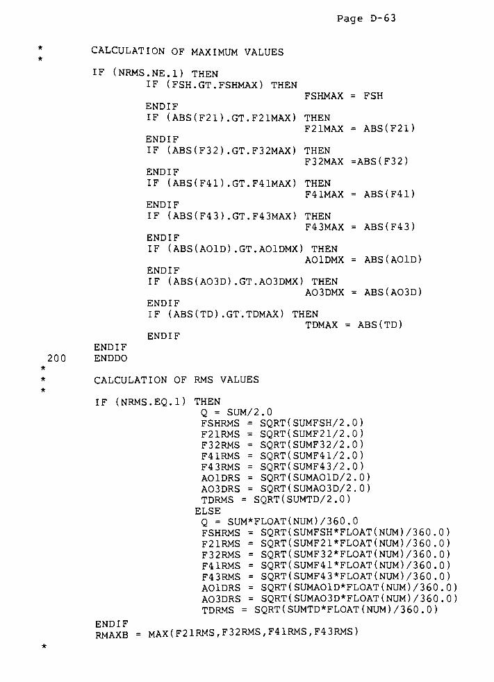
Page D-63
*
*
CALCULATION OF MAXIMUM VALUES
IF (NRMS.NE.l) THEN
IF ( FSH. GT. FSHMAX) THEN
FSHMAX = FSH
ENDIF
IF (ABS(F21) .GT.F21MAX) THEN
F21MAX = ABS(F21)
ENDIF
IF (ABS(F32) .GT.F32MAX) THEN
F32MAX =ABS(F32)
ENDIF
IF (ABS(F41) .GT.F41MAX) THEN
F41MAX = ABS(F41)
ENDIF
IF (ABS(F43) .GT.F43MAX) THEN
F43MAX = ABS(F43)
ENDIF
IF ( ABS ( AOID ) .GT. AOIDMX ;) THEN
AOIDMX = ABS(AOID)
ENDIF
IF (ABS(A03D) .GT.A03DMX) THEN
A03DMX = ABS(A03D)
ENDIF
IF ( ABS ( TD ) .GT. TDMAX) THEN
TDMAX == ABS(TD)
ENDIF
ENDIF
200*
ENDDO
*
*
CALCULATION OF RMS VALUES
IF (NRMS.EQ. 1 THEN
Q = SUM/2.0
FSHRMS = SQRT
F21RMS = SQRT
F32RMS = SQRT
F41RMS = SQRT
F4 3RMS = SQRT
AOIDRS = SQRT
A03DRS = SQRT
TDRMS = SQRT(
ELSE
Q = SUM*FLOAT
FSHRMS = SQRT
F21RMS = SQRT
F32RMS = SQRT
F41RMS = SQRT
F4 3RMS = SQRT
AOIDRS = SQRT
A03DRS = SQRT
TDRMS = SQRT(
(SUMFSH/2.0)
(SUMF21/2.0)
(SUMF32/2.0)
(SUMF41/2.0)
(SUMF43/2.0)
(SUMAO1D/2.0)
(SUMAO3D/2.0)
SUMTD/2.0)
( NUM )/3 60.0
(SUMFSH*FLOAT(NUM)/360.0)
(SUMF21*FLOAT(NUM)/360.0)
(SUMF32*FLOAT(NUM)/360.0)
(SUMF41*FLOAT(NUM)/360.0)(SUMF4 3*FLOAT(NUM)/360.0)(SUMAOID* FLOAT ( NUM) /3 60.0)
(SUMAO3D*FLOAT(NUM)/360.0)SUMTD*FLOAT (NUM) /360 . 0 )
ENDIF
RMAXB = MAX(F21RMS,F32RMS,F41RMS,F43RMS)
*
*
*
Page D-64
REGIONAL CONSTRAINTS
RMAXH = MAX ( AOIDRS, A03DRS)DO 250 I = 1,6
R(I) = V(I)
R(I + 6) = 1.0 - V(I)250 ENDDO
R(13) = CG(26) - FSHRMS
R(14) = CG(27) - RMAXB
R(15) = CG(28) - RMAXH
R(16) = CG(29) - TDRMS
DO 260 I = 1,NR
RR(I) = R(I) ! RR(I) IS COMMON
260 ENDDO
*
* DETERMINATION OF THE PENALIZED OPTIMZATION FUNCTION*
*
B = 0.
H = 0.
IF(NE.EQ.O) THEN
GO TO 300"
ENDIF
DO 310 IE = 1,NE
B = B + E(IE)* E(IE)
310 ENDDO
300 IF (NR.EQ.0) THEN
GO TO 3 50
ENDIF
DO 320 IR = 1,NR
IF (R(IR) .LT.0. ) THEN
H = H + R(IR)*R(IR)
ENDIF
320 ENDDO
350 W = B + H
P = CP * FP * W ! PENALTY FUNCTION
x = q + p ! PENALIZED OPTIMIZATION QUANTITY
RETURN
END
************************************************************************

Page D-65
*****
*
*
*
*
*****
*
*
*
*
*
*****
*
*
*
*
*
*
*
*
*
*
*
*
*
*
*
*
*
*
*
*
*
*
*
*
*
*
*
*
*
*
*
*
*
*
*
*
*
*
*
*
*
*
*
**************FINAL ITEMS SUBROUTINE
***********************
THIS SUBROUTINE PRINTS OUT ALL THE FINAL RESULTS FOR THE
OPTIMIZATION STUDY.
*****************SUBROUTINES CALLED
***********************
SUBROUTINE PRINT(I)-
PRINTS A ROW OF CHARACTERS DEFINED BY I .
ie. IF I = 1 THEN A ROW OF"*"
WILL BE PRINTED
******************VARIABLES USED
*************************
AOiD
AOiDMAX
AP
AOiDRMS
AU
C
CG
CG(24)
CG(25)
E
FijFijX
FijY
F i jMAX
Fij RMS
FSH
FSHMAX
FSHRMS
G
LC
N
NC
NGQ
NE
NF
NR
NRMS
NU
OI
P
Q
RR
RMAXB
RMAXH
TD
THTC
U
V
TIME DERIVATIVE OF THE TOTAL ANGULAR MOMENTUM OF
THE MECHANISM WITH RESPECT TO THE JOINT Oi.
THE MAXIMUM AOiD IN ONE REVOLUTION OF THE INPUT L
VALUE OF PI (3.14159) .
RMS VALUE OF AOiD.
DIFFERENCE IN THE LIMITS OF INTEGRATION.
MATRIX OF CALCULATED CONSTANTS (NOT USED).
MATRIX OF GIVEN CONSTANTS.
MAXIMUM COUNTERWEIGHT ANGLE (I.E. 2*PI).
MAXIMUM C.W. RADIUS (IN).
MATRIX OF EQUALITY CONSTRAINTS (NOT USED).
FINAL ITEMS MATRIX.
THE NORMALIZED BEARING FORCE BETWEEN LINKS i AND j"X"
COMPONET OF THE FORCE Fij."Y"
COMPONET OF THE FORCE Fij.
MAXIMUM Fij FORCE.
RMS Fij.
SHAKING FORCE OF THE MECHANISM.
MAXIMUM SHAKING FORCE.
RMS SHAKING FORCE.
ABS I CCA OF THE SAMPLING POINT; USED IN GAUSSIAN.
QUADRATURE INTEGRATION.
RADIUS OF THE iTH COUNTERWEIGHT .( IN)
NOT USED.
NUMBER OF COUNTERWEIGHTS TO BE ADDED ( 1 < NC < 3
NUMBER OF SAMPLING POINTS FOR NUMERICAL INTEGRATI"
EQUALITY CONSTRAINTS."
FINAL ITEMS
NUMBER OF REGIONAL CONSTRAINTS.
DETERMINES THE TYPE OF INTEGRATION USED.
NUMBER OF VARIABLES IN MATRIX U (NOT USED).
NOT USED .
PENALTY FUNCTION.
OBJECTIVE FUNCTION .
REGIONAL CONSTRAINT MATRIX.
THE MAXIMUM RMS FORCE.
THE MAXIMUM RMS SHAKING MOMENT.
NORMALIZED DRIVING (INPUT) TORQUE.
ANGLE BETWEEN LI NIK i AND THE iTH COUNTERWEIGHT.
NOT USED.
SCALED VARIABLES ; ANGLES AND RADII OF THE
COUNTERWEIGHTS.
*****
*
*
*
*
*****
*
*
*
*
*
*****
*
*
*
INK.*
*
*
*
*
*
*
*
*
*
*
*
*
*
*
*
*
*
*
*
*
*
*
*
*
*
*
*
*
*
*
*
*
*
*
*
*
*
*
*
).
ON.

Page D-66
*ZZ : WEIGHTING COEFFICIENTS FOR GAUSSIAN QUADRATURE
*
*
INTEGRATION.*
* *
****************MAIN SUB-PROGRAM
************************************
*
*
*
*
SUBROUTINE FINAL (MAXN, C, CG, F,Q,U,V,KC,NF,NU,NV)REAL * 8 C(MAXN),CG(MAXN),F(MAXN),G(24),RR(19),U(MAXN),V(MAXN),
S< ZZ(24) ,Q,AP, FSHMAX, F21MAX, F32MAX, F41MAX, F43MAX, AOIDMX,& A03DMX
, TDMAX, FSHRMS , F2 1RMS , F3 2RMS ,
F4 1RMS ,F4 3RMS ,
AOIDRS ,
& A03DRS,TDRMS
INTEGER * 4 NC,NF ,NU ,NV,NRMS,NR
COMMON G, ZZ , RR , AP , FSHMAX
,F2 1MAX
,F 3 2MAX
,F4 1MAX
,F4 3MAX
,AOIDMX
,
Sc A03DMX, TDMAX
, FSHRMS,F2 1RMS
,F32RMS
,F4 1RMS , F43RMS ,
S. AOIDRS , A03DRS , TDRMS/A1/NRMS , NC , NGQ ,NR
HERE USER PROGRAMS FINAL EQUATIONS OF INTEREST
F(l)= Q
F(2)=CG(24)*V(1)
F(3)=CG(24)*V(2)
F(4)=CG(24)*V(3)
F(5)=CG(25)*V(4)
F(6)=CG(25)*V(5)
F(7)=CG(25)*V(6)
WRITEU, 601)
WRITE(7,601)
601 FORMAT(//2 5X,'
OPTIMUM VARIABLES',//,8X,' THTC1',4X,'
THTC2'
,
Sc4X,' THTC3',5X,' LC1',6X,' LC2',6X,'
LC3*,//)
WRITEU, 602) (F(JF) ,JF=2,NF)
WRITE(7,602) ( F( JF) ,JF=2 ,NF)
602 FORMAT(4X,6(4X,F6.3) ,//)
DO 100 I = 1,NR
IF (RR(I) .LT.0.0) THEN
WRITE(6,603) I,RR(I)
ELSE
WRITE(7,603) I,RR(I)
WRITE(6,604) I,RR(l)
WRITE(7,604) I,RR(I)
ENDIF
100 ENDDO
WRITE(6,605)
WRITE(7,605)
WRITE(6,606)
WRITE(7,606)
WRITE ( 6 ,60 7 ) FSHRMS
,F2 1RMS ,
F3 2RMS ,F4 1RMS ,
F4 3RMS ,
& AOIDRS, A03DRS, TDRMS
WRITE ( 7 ,607 ) FSHRMS ,
F2 1RMS ,F32RMS
,F4 1RMS
,F4 3RMS
,
& AOIDRS, A03DRS, TDRMS
WRITEU, 608)
WRITE(7,608)
WRITEU, 609)
WRITE(7,609)
WRITE (6, 610) FSHMAX, F21MAX, F32MAX, F41MAX, F4 3MAX,
&A01DMX,A03DMX,TDMAX

*
*.
Page D-67
WRITE (7, 610) FSHMAX, F21MAX, F32MAX, F41MAX, F43MAX,& AO 1DMX
, AO3DMX,TDMAX
603 FORMAT (10X,' REGIONAL CONSTRAINT #',13,'
WAS VIOLATED :',E14.7)
604 FORMATU0X,'REGIONAL CONSTRAINT #
',13,'
WAS OBEYED :',E14.7)
605 FORMAT (//, 2 5X,'
RMS VALUES ',//)606 FORMAT(2X,'
FSH',4X,'
F21',4X,'
F32',4X,'
F41*,4X,'
F43 ',& 4X,'
AOID',3X,'
A03D',3X,'
TD ',//)607 F0RMAT(1X,8(F5.3,4X),//)608 F0RMAT(//,25X,
*
MAXIMUM VALUES ',//)609 FORMAT(2X,'
FSH',4X,'
F21',4X,'
F32',4X,'
F41',4X,'
F43 ',Sc 4X,'
AOID\3X,'
A03D',3X,'
TD ',//)610 F0RMAT(1X,8(F6.3,3X) ,//)
CALL PRINT(l) ! PRINTS A ROW OF"*"
WRITEU,*)'
FINAL ITEMS F(JF) FOR JF = 1, ,NF ARE =
WRITEU, 611) (F(JF),JF=1,NF)611 FORMAT(/,4(3X,E14.7) )
RETURN
END

Page D-68
************************ GAUSS QUADRATURE INTEGRATION*****************
*THIS SUBROUTINE PROVIDES DOUBLE PRECISION NUMBERS FOR GAUSSIAN *
*QUADRATURE INTEGRATION. A MAXIMUM OF 10 SAMPLING POINT CAN
*
* CAN BE CHOOSEN .
*
* *
************************ DEFINITION OF VARIABLES**********************
* *
* M : # OF SAMPLING POINTS*
* G : ABS I CCA VALUE OF THE SAMPLING POINT,
M*
* ZZ : THE WEIGHTING COEFFICIENT ASSOCIATED WITH THE*
*SAMPLING POINT ,M
*
*
* *
*********************** ^A j ^ PROGRAM********************************
* *
SUBROUTINE PGAUSS (M)REAL * 8 G(24) ,ZZ(24)
COMMON G,ZZ
GO TO (1,2,3,4,5,6,7,8,9,-10,11,12,13,14,15,16,17,18,19,20,21,Sc 22, 23, 24), M
1 G(l) = 0.0
ZZ(1) = 2.0
RETURN
2 G(l) = 1.0/SQRT(3.0)
G(2) =-G(l)
ZZ(1) = 1.0
ZZ(2) = 1.0
RETURN
3 G(l) = SQRT (0.6)
G(2) = 0.0
G(3) =-G(l)
ZZ(1) = 5./9.
ZZ(2) = 8./9.
ZZ(3) = ZZ(1)
RETURN
4 G(l) = 0.861136311594053
G(2) = 0.339981043584856
G(3) =-G(2)
GU) =-G(l)
ZZ(1) = 0.347854845137454
ZZ(2) = 0.652145154862546
ZZ(3) = ZZ(2)
ZZ(4) = ZZ(1)
RETURN
5 G(l) = 0.906179845938664
G(2) = 0.538469310105683
G(3) = 0.0
GU) = - G(2)
G(5) = -G(l)
ZZ(1) = 0.236926885056189
ZZ(2) = 0.478628670499366
ZZ(3) = 0.568888888888889
ZZU) = ZZ(2)
ZZ(5) = ZZ(1)
Page D-69
RETURN
G(l) =
0.932469514203152G 2) =
0.661209386466265G 3) =
0.238619186083197GU) =
-G(3)
G(5) =
-Q(2)
G(6) =
-G(l)
ZZ(1) =
0.171324492379170ZZ(2) =
0.360761573048139ZZ(3) =
0.467913934572691ZZ(4) =
ZZ(3)
ZZ(5) = ZZ(2)
ZZ(6) = ZZ(1)
RETURN
G(l) =
0.949107912342759G(2) = 0.741531185599394G(3) = 0.405845151377397G(4) = 0.0
G(5) =-G(3)
GU) =-G(2)
G(7) =-G(l)
ZZ(1) = 0.129484966168870ZZ(2) = 0.279705391489277ZZ(3) = 0.381830050505119ZZ(4) = 0.417959183673469ZZ(5) = ZZ(3)
ZZ(6) = ZZ(2)
ZZ(7) = ZZ(1)
RETURN
G(l) = 0.960289856497536
G(2) = 0.796666477413627
G(3) = 0.525532409916329
G(4) = 0.183434642495650
G(5) =-GU)
G(6) =-G(3)
G(7) =-G(2)
G(8) =-G(l)
ZZ(1) = 0.101228536290376
ZZ(2) = 0.222381034453374
ZZ(3) = 0.313706645877887
ZZU) = 0.362683783378362
ZZ(5) = ZZU)
ZZ(6) = ZZ(3)
ZZ(7) = ZZ(2)
ZZ(8) = ZZ(1)
RETURN
G(l) = 0.968160239507626
G(2) = 0.836031107326636
G(3) = 0.613371432700590
G(4) = 0.324253423403809
G(5) = 0.0
GU) =-GU)
G(7) =-G(3)
G(8) =-G(2)
G(9) =-G(l)

Page D-70
ZZ(1) = 0.081274388361574
ZZ(2) = 0.180648160694857
ZZ(3) = 0.260610696402935
ZZ(4) = 0.312347077040003
ZZ(5) = 0.330239355001260
ZZ(6) = ZZU)
ZZ(7) = ZZ(3)
ZZ(8) = ZZ(2)
ZZ(9) = ZZ(1)
RETURN
lO G(l) = 0.973906528517172
G(2) = 0.865063366688985
G(3) = 0.679409568299024
G(4) = 0.433395394129247
G(5) = 0.148874338981631
G(6) =-G(5)
G(7) =-GU)
G(8) =-G(3)
G(9) =-G(2)
G(10) =-G(l)
ZZ(1) = 0.066671344308688
ZZ(2) = 0.149451349150581
ZZ(3) = 0.219086362515982
ZZ(4) = 0.269266719309996
2Z(5) - 0.295524224714753
ZZ(6) = ZZ(5)
ZZ(7) = ZZ(4)
ZZ(8) =: ZZ(3)
ZZ(9) == ZZ(2)
ZZ(10) = ZZ(1)
RETURN
11 WRITE (6,,*)*
NGQ =11 NOT AVAILABLE
RETURN
12 G(l) = 0.981560634246719
G(2) = 0.904117256370475
G(3) = 0.769902674194305
G(4) = 0.587317954286617
G(5) = 0.367831498998180
GU) = 0.125233408511469
G(7) = -GU)
G(8) = -G(5)
G(9) = -GU)
G(10)= -G(3)
G(ll)= -G(2)
G(12)= -G(l)
ZZ(1)= 0.047175336386512
ZZ(2)= 0.106939325995318
ZZ(3)= 0.160078328543346
ZZ(4)= 0.203167426723066
ZZ(5)= 0.233492536538355
ZZ(6)= 0.249147045813403
ZZ(7)= ZZ(6)
ZZ(8)= ZZ(5)
ZZ(9)= ZZ(4)
ZZ(10)=ZZ(3)
Page D-71
ZZ(11)=ZZ(2)
ZZ(12)=ZZ(1)RETURN
13 WRITEU,*)'
RETURN
14 WRITEU,*)'
RETURN
15 WRITEU,*)'
RETURN
16 G(l) =
G(2) =
G(3) =
G(4) =
G(5) =
G(6) =
G(7) =
G(8) =
G(9) =
G(10)=
G(ll)=
G(12)=
G(13)=
G(14)=
G(15)=
G(16)=
ZZ(1)=
ZZ(2)=
ZZ(3)=
ZZ(4)=
ZZ(5)=
ZZ(6)=
ZZ(7)=
ZZ(8)=
ZZ(9)=
ZZ(10)=ZZ(7)
ZZ(11)=ZZ(6)
ZZ(12)=ZZ(5)
ZZ(13)=ZZ(4)
ZZ(14)=ZZ(3)
ZZ(15)=ZZ(2)
ZZ(16)=ZZ(1)
RETURN
17 WRITEU,*)'
RETURN
18 WRITEU,*)'
RETURN
19 WRITEU,*)'
RETURN
20 G(l) =
NGQ =13 NOT AVAILABLE
NGQ =14 NOT AVAILABLE
NGQ =15 NOT AVAILABLE
0.9894009349916499325960.94457 502 307 32 32 576078
0.8656312023878 3174 3880
0.755404408355003033895
0.61787624440264 37484470.4 58016777657 227 38634 2
0.28160 3550779258913230
0.095012509837 637440185
-G(8)
-G(7)
-GU)
-G(5)
-GU)
-G(3)
-G(2)
-G(l)
"
0.0271524594117 54094852
062253523938647892863
095158511682492784610
124628971255533872052
149595988816576732081
169156519395002538189
182603415044923588867
189450610455068496285
0
0
0.
0
0
0
0
ZZ(8)
NGQ =17 NOT AVAILABLE
NGQ =18 NOT AVAILABLE
NGQ =19 NOT AVAILABLE
0.993128 599185094924786
G(2) = 0.963971927277913791268
G(3) = 0.912234428251325905868
GU) = 0.839116971822218823395
G(5) = 0.746331906460150792614
G(6) = 0.636053680726515025453
G(7) = 0.510867001958827098004

Page D-72
21
22
23
24
G(8)
G(9)
G(10
G(ll
G(12
G(13
G(14
G(15
G(16
G(17
G(18
G(19
G(20
ZZ(1
ZZ(2
ZZ(3
ZZ(4
ZZ(5
ZZ(6
ZZ(7
ZZ(8
=
0.373706088715419560673=
0.227785851141645078080=
0.076526521133497333755=
-G(10)
=
-G(9)
=
-G(8)
=
-G(7)
=
-G(6)
=
~G(5)
=
-GU)
=
-G(3)
=
-G(2)
=-G(l)
=
0.017614007139152118312=
0.040601429800386941331=
0.062672048334109063570=
0.083276741576704748725=
0.101930119817240435037=
0.118194531961518417312=
0.131688638449176626898=
0.1420961093183820513290.1491729864726037467880.152753387130725850698
ZZ(9
ZZ(10)=
ZZ(11)=ZZ(10)
ZZ(12)=ZZ(9)
ZZ(13)=ZZ(8)
ZZ(14)=ZZ(7)
ZZ(15)=ZZ(6)
ZZ(16)=ZZ(5)
ZZ(17)=ZZ(4)
ZZ(18)=ZZ(3)
ZZ(19)=ZZ(2)
ZZ(20)=ZZ(1)
RETURN
WRITE(6,*)'
RETURN
WRITEU,*)'
RETURN
WRITEU,*)*
RETURN
NGQ =21 NOT AVAILABLE
NGQ 2 2 NOT AVAILABLE
NGQ =23 NOT AVAILABLE
G(l) =
G(2) =
G(3) =
GU) =
G(5) =
G(6) =
G(7) =
G(8) =
G(9) =
G(10)=
G(ll)=
G(12)=
G(13) = -
G(14) = -
G(15) = -
0
0
0,
0,
0,
0,
0,
0.
0.
0.
0.
0.
995187219997021360180
974728555971309498198
938274552002732758524
886415527004401034213
820001985973902921954
740124191578554364244
648093651936975569252
545421471388839535658
433793507626045138487
315042679696163374387
191118867473616309159
0640568 9286260562608 5
G(12)
G(ll)
G(10)
Page D-73
G(16) = -
G(9)
G(17) = -
G(8)
G(18) = -
G(7)
G(19) = -
GU)
G(20) = -
G(5)
G(21) = -
GU)
G(22) = -
G(3)
G(23) = -
G(2)
G(24) = -
G(l)
ZZ(1) = 0.012341229799987199547
ZZ(2) = 0.028531388628933663181
ZZ(3) = 0.044277438817419806169
ZZU) = 0.059298584915436780746
ZZ(5) = 0.073346481411080305734
ZZ(6) = 0.086190161531953275917
ZZ(7) = 0.097618652104113888270
ZZ(8) = 0.107444270115965634763
ZZ(9) = 0.115505668053725601353
ZZ(10)= 0.121670472927803391204
ZZ(11)= 0.125837456346828296121
ZZ(12)= 0.127938195346752156794
ZZ(13)= ZZ(12)
ZZ(14)= ZZ(ll)
ZZ(15)= ZZ(10)
ZZ(16)= ZZ(9)
ZZ(17)= ZZ(8)
ZZ(18)= ZZ(7)
ZZ(19)= ZZ(6)
ZZ(20)= ZZ(5)
ZZ(21)= ZZ(4)
ZZ(22)= ZZ(3)
ZZ(23)= ZZ(2)
ZZ(24)= ZZ(1)
RETURN
END