aws july webinar series: amazon redshift optimizing performance
TRANSCRIPT

© 2015, Amazon Web Services, Inc. or its Affiliates. All rights reserved.
Sanjay Kotecha, Solution ArchitectEric Ferreira, Principal Database Engineer
July 21, 2015
Best Practices: Amazon Redshift
Optimizing Performance

Getting Started – June Webinar Series: https://www.youtube.com/watch?v=biqBjWqJi-Q
Best Practices – July Webinar Series:
Optimizing Performance – July 21, 2015
Migration and Data Loading – July 22,2015
Reporting and Advanced Analytics – July 23, 2015
Amazon Redshift – Resources
Architecture
Distribution
Sort Keys
Compression
DDL
Loading
Vacuum
Analyze
Workload Management
Agenda
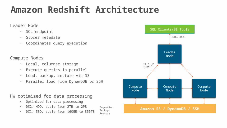
Leader Node• SQL endpoint
• Stores metadata
• Coordinates query execution
Compute Nodes• Local, columnar storage
• Execute queries in parallel
• Load, backup, restore via S3
• Parallel load from DynamoDB or SSH
HW optimized for data processing• Optimized for data processing
• DS2: HDD; scale from 2TB to 2PB
• DC1: SSD; scale from 160GB to 356TB
10 GigE(HPC)
IngestionBackupRestore
SQL Clients/BI Tools
128GB RAM
16TB disk
16 cores
Amazon S3 / DynamoDB / SSH
JDBC/ODBC
128GB RAM
16TB disk
16 coresCompute Node
128GB RAM
16TB disk
16 coresCompute Node
128GB RAM
16TB disk
16 coresCompute Node
LeaderNode
Amazon Redshift Architecture
128GB RAM
16TB disk
16 cores
128GB RAM
16TB disk
16 coresLeader Node
128GB RAM
16TB disk
16 cores
RAM
CPU
RAM
CPU
RAM
CPU
RAM
CPU
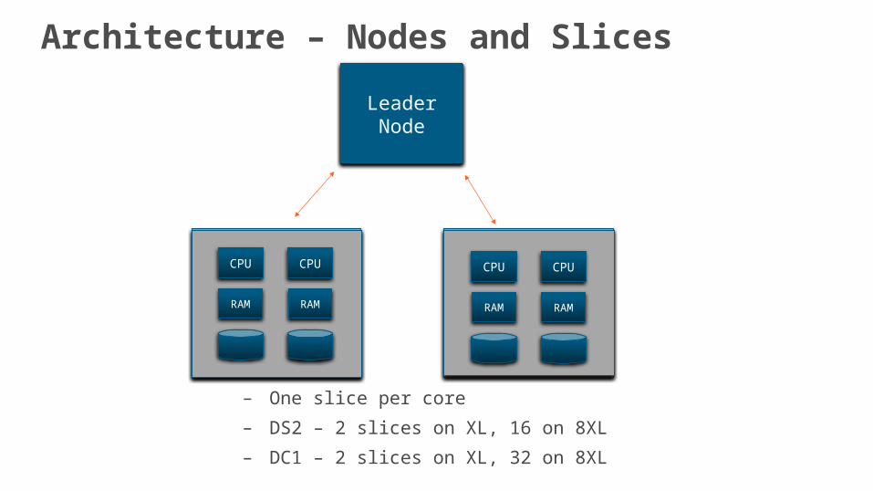
– One slice per core
– DS2 – 2 slices on XL, 16 on 8XL
– DC1 – 2 slices on XL, 32 on 8XL
Architecture – Nodes and Slices
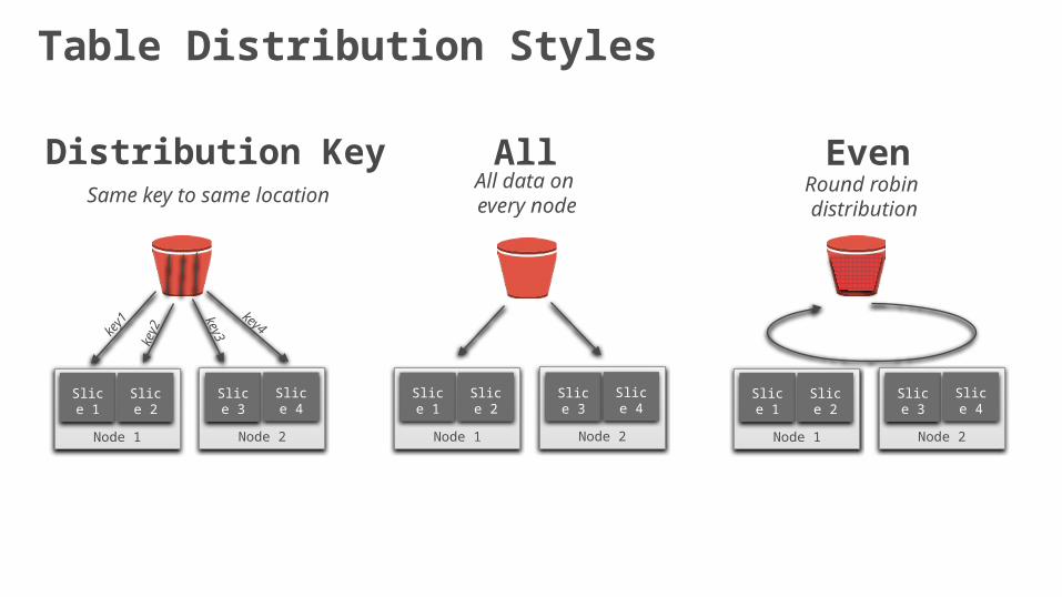
Table Distribution Styles
Distribution Key All
Node 1
Slice 1
Slice 2
Node 2
Slice 3
Slice 4
Node 1
Slice 1
Slice 2
Node 2
Slice 3
Slice 4
key1
key2
key3
key4
All data on every nodeSame key to same location
Node 1
Slice 1
Slice 2
Node 2
Slice 3
Slice 4
EvenRound robin distribution
Node 1
Slice 1 Slice 2
Node 2
Slice 3 Slice 4
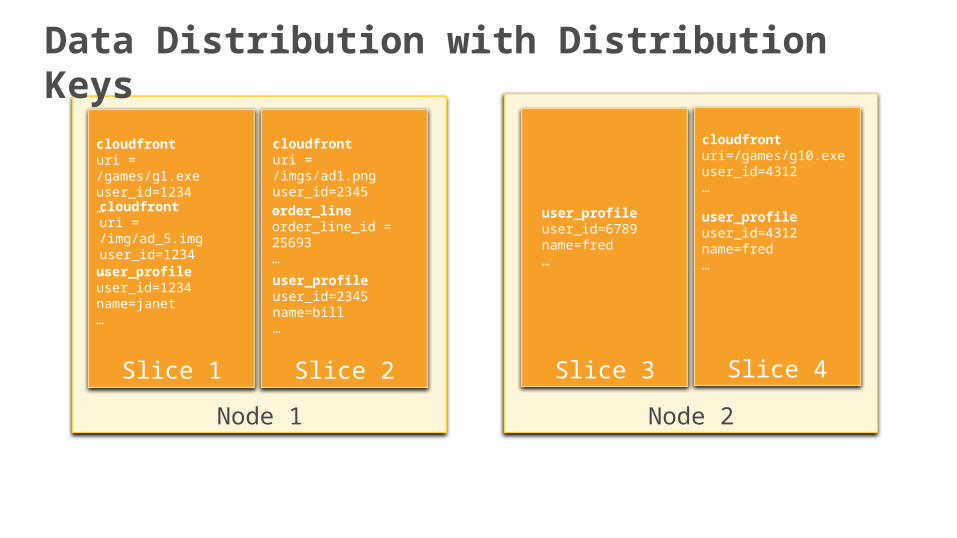
cloudfronturi = /games/g1.exeuser_id=1234…
user_profileuser_id=1234name=janet…
user_profileuser_id=6789name=fred…
cloudfronturi = /imgs/ad1.pnguser_id=2345…
user_profileuser_id=2345name=bill…
cloudfronturi=/games/g10.exeuser_id=4312…
user_profileuser_id=4312name=fred…
order_lineorder_line_id = 25693…
cloudfronturi = /img/ad_5.imguser_id=1234…
Data Distribution with Distribution Keys
Node 1
Slice 1 Slice 2
Node 2
Slice 3 Slice 4
user_profileuser_id=1234name=janet…
user_profileuser_id=6789name=fred…
cloudfronturi = /imgs/ad1.pnguser_id=2345…
user_profileuser_id=2345name=bill…
cloudfronturi=/games/g10.exeuser_id=4312…
user_profileuser_id=4312name=fred…
order_lineorder_line_id = 25693…
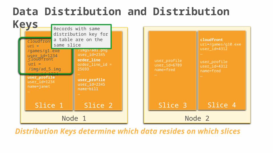
Distribution Keys determine which data resides on which slices
cloudfronturi = /games/g1.exeuser_id=1234…cloudfronturi = /img/ad_5.imguser_id=1234…
Records with same distribution key for a table are on the same slice
Data Distribution and Distribution Keys
Node 1
Slice 1 Slice 2
cloudfronturi = /games/g1.exeuser_id=1234…
user_profileuser_id=1234name=janet…
cloudfronturi = /imgs/ad1.pnguser_id=2345…
user_profileuser_id=2345name=bill…
order_lineorder_line_id = 25693…
cloudfronturi = /img/ad_5.imguser_id=1234…
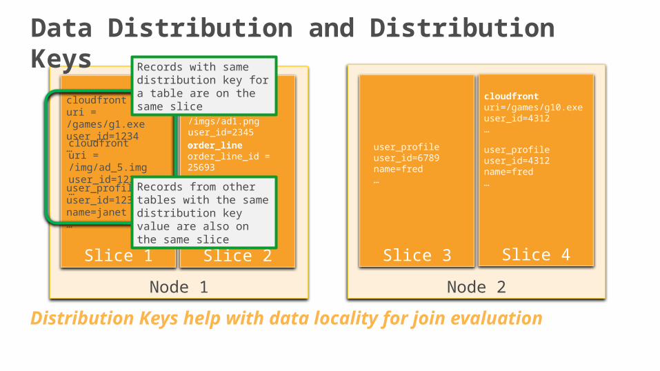
Records from other tables with the same distribution key value are also on the same slice
Records with same distribution key for a table are on the same slice
Distribution Keys help with data locality for join evaluation
Node 2
Slice 3 Slice 4
user_profileuser_id=6789name=fred…
cloudfronturi=/games/g10.exeuser_id=4312…
user_profileuser_id=4312name=fred…
Data Distribution and Distribution Keys
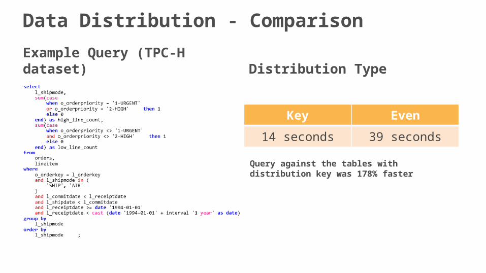
Example Query (TPC-H dataset)
Data Distribution - Comparison
Distribution Type
Query against the tables with distribution key was 178% faster
Key Even
14 seconds 39 seconds
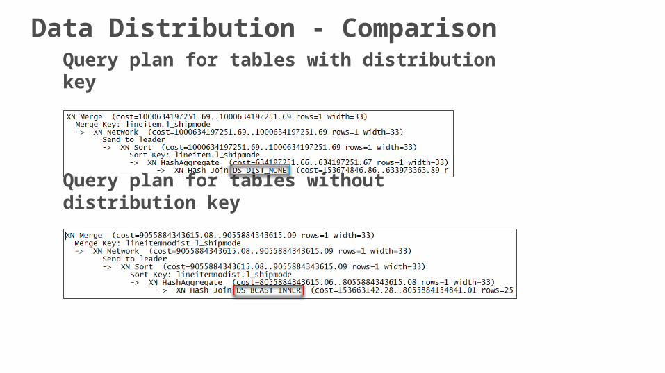
Query plan for tables with distribution key
Data Distribution - Comparison
Query plan for tables without distribution key
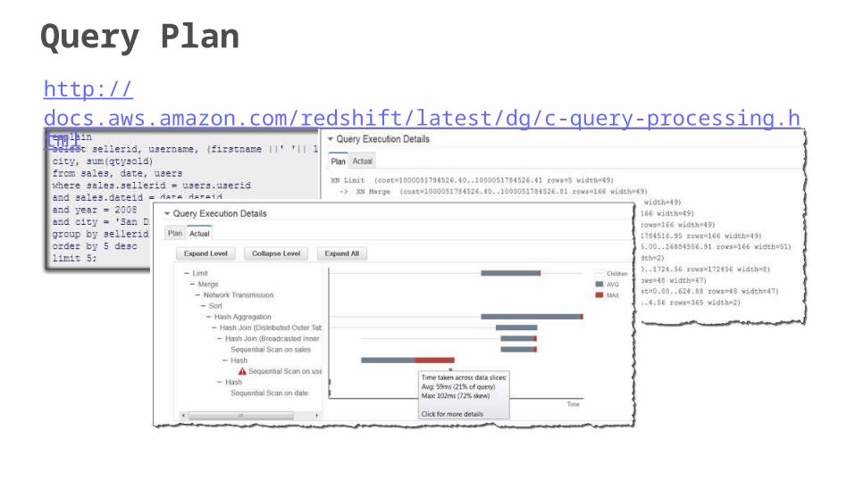
Query Plan
http://docs.aws.amazon.com/redshift/latest/dg/c-query-processing.html
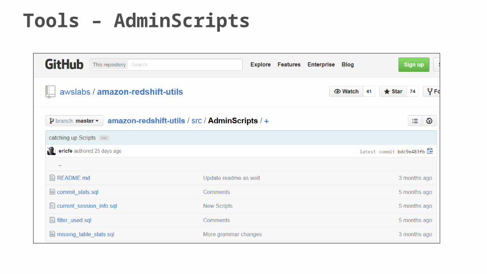
Tools – AdminScripts
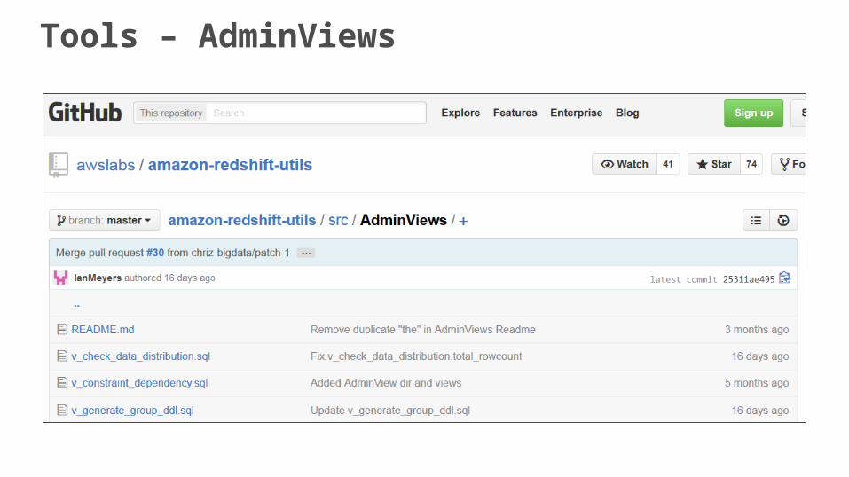
Tools – AdminViews
Node 1
Slice 1 Slice 2
Node 2
Slice 3 Slice 4
cloudfronturi = /games/g1.exeuser_id=1234…
cloudfronturi = /imgs/ad1.pnguser_id=2345…
cloudfronturi=/games/g10.exeuser_id=4312…
cloudfronturi = /img/ad_5.imguser_id=1234…
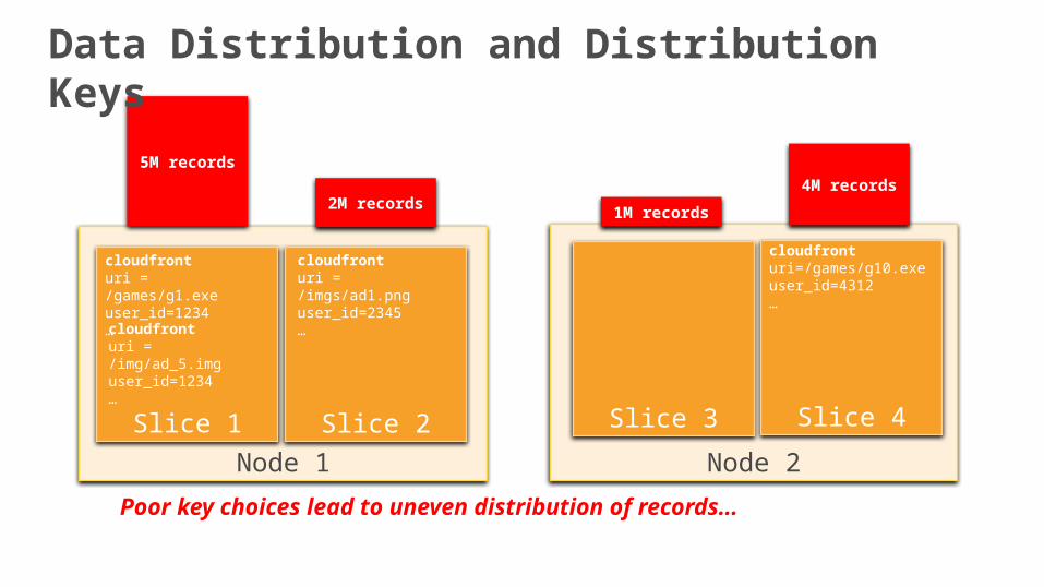
2M records
5M records
1M records
4M records
Poor key choices lead to uneven distribution of records…
Data Distribution and Distribution Keys
Node 1
Slice 1 Slice 2
Node 2
Slice 3 Slice 4
cloudfronturi = /games/g1.exeuser_id=1234…
cloudfronturi = /imgs/ad1.pnguser_id=2345…
cloudfronturi=/games/g10.exeuser_id=4312…
cloudfronturi = /img/ad_5.imguser_id=1234…
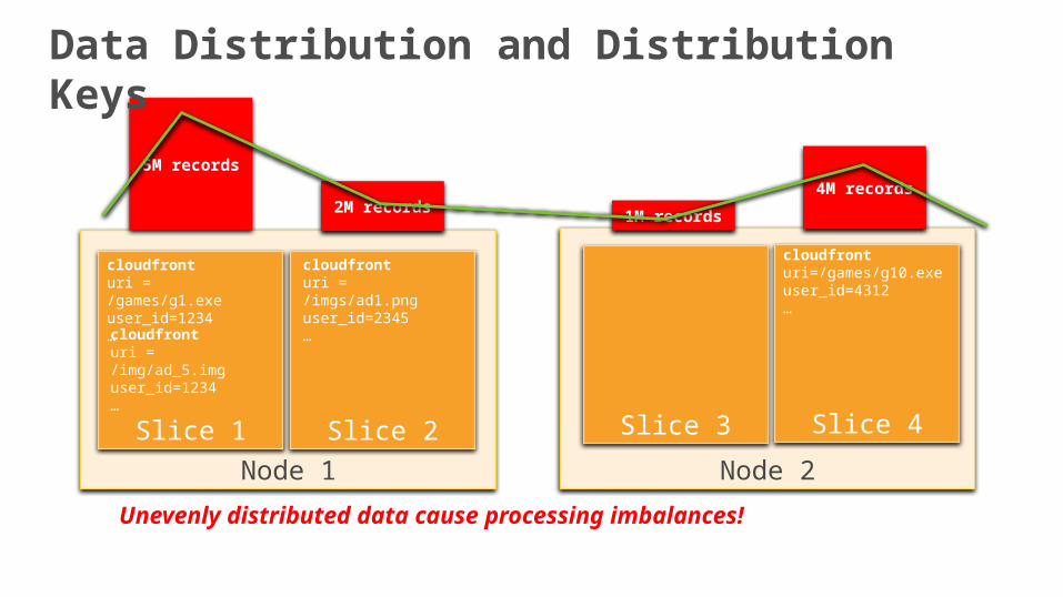
2M records
5M records
1M records
4M records
Unevenly distributed data cause processing imbalances!
Data Distribution and Distribution Keys
Node 1
Slice 1 Slice 2
Node 2
Slice 3 Slice 4
cloudfronturi = /games/g1.exeuser_id=1234…
cloudfronturi = /imgs/ad1.pnguser_id=2345…
cloudfronturi=/games/g10.exeuser_id=4312…
cloudfronturi = /img/ad_5.imguser_id=1234…
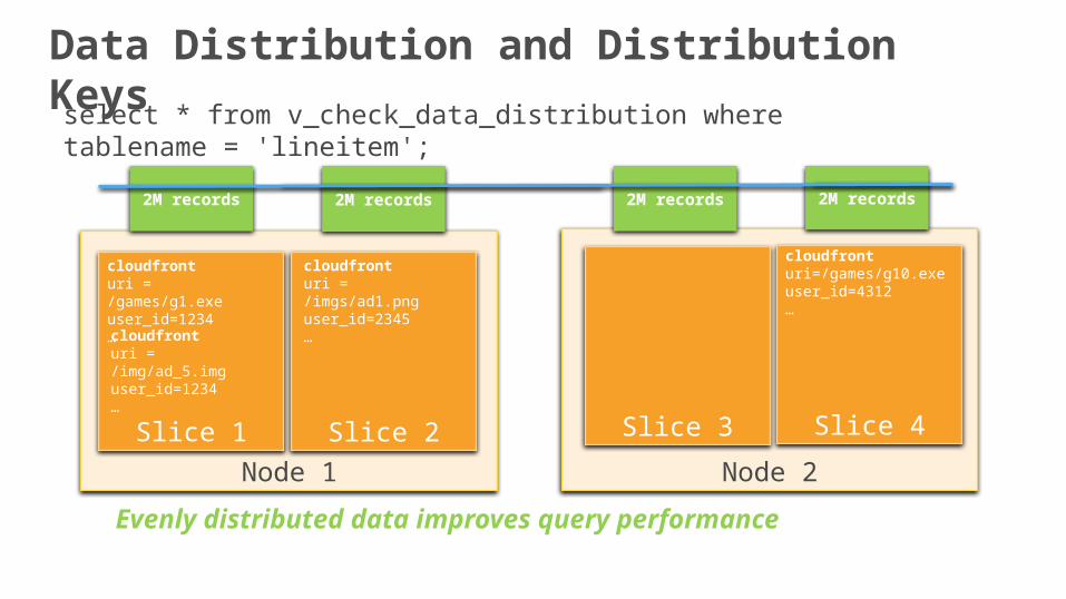
2M records2M records 2M records 2M records
Evenly distributed data improves query performance
select * from v_check_data_distribution where tablename = 'lineitem';
Data Distribution and Distribution Keys
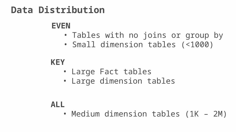
KEY• Large Fact tables• Large dimension tables
ALL • Medium dimension tables (1K – 2M)
EVEN• Tables with no joins or group by• Small dimension tables (<1000)
Data Distribution
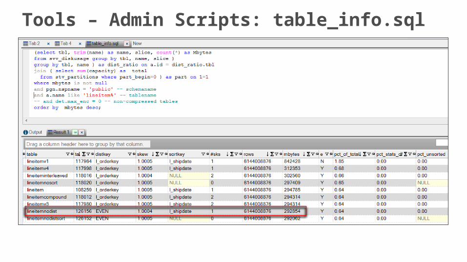
Tools – Admin Scripts: table_info.sql
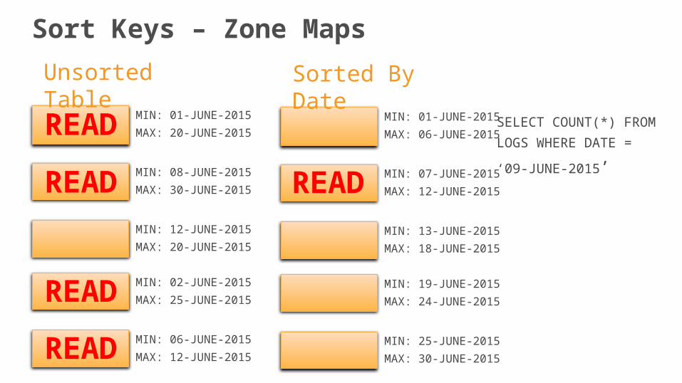
SELECT COUNT(*) FROM
LOGS WHERE DATE = ‘09-
JUNE-2015’
MIN: 01-JUNE-2015
MAX: 20-JUNE-2015
MIN: 08-JUNE-2015
MAX: 30-JUNE-2015
MIN: 12-JUNE-2015
MAX: 20-JUNE-2015
MIN: 02-JUNE-2015
MAX: 25-JUNE-2015
MIN: 06-JUNE-2015
MAX: 12-JUNE-2015
Unsorted Table
MIN: 01-JUNE-2015
MAX: 06-JUNE-2015
MIN: 07-JUNE-2015
MAX: 12-JUNE-2015
MIN: 13-JUNE-2015
MAX: 18-JUNE-2015
MIN: 19-JUNE-2015
MAX: 24-JUNE-2015
MIN: 25-JUNE-2015
MAX: 30-JUNE-2015
Sorted By Date
READ
READ
READ
READ
READ
Sort Keys – Zone Maps
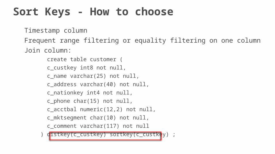
Sort Keys - How to choose
Timestamp column
Frequent range filtering or equality filtering on one column
Join column: create table customer (
c_custkey int8 not null,
c_name varchar(25) not null,
c_address varchar(40) not null,
c_nationkey int4 not null,
c_phone char(15) not null,
c_acctbal numeric(12,2) not null,
c_mktsegment char(10) not null,
c_comment varchar(117) not null
) distkey(c_custkey) sortkey(c_custkey) ;
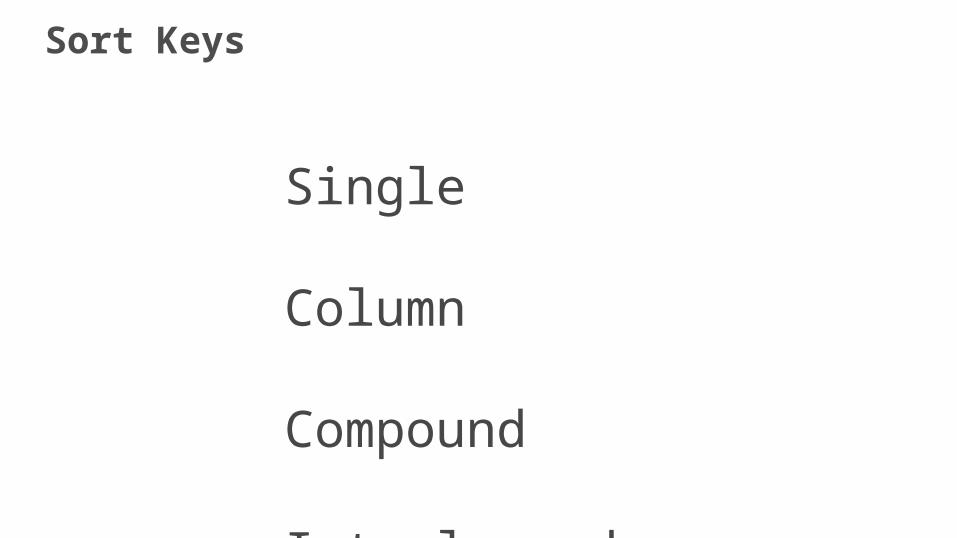
Single Column
Compound
Interleaved
Sort Keys
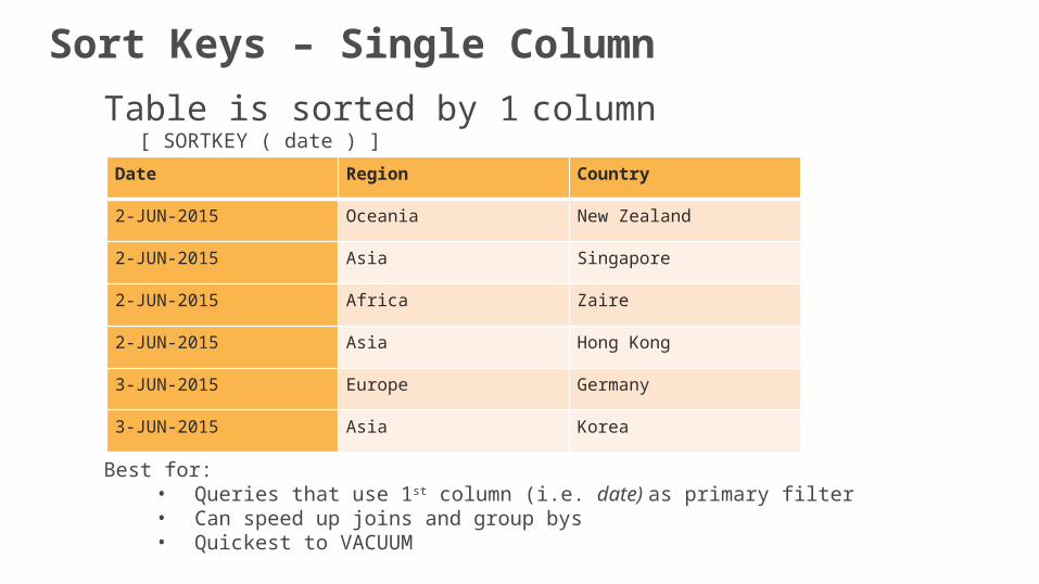
Table is sorted by 1 column[ SORTKEY ( date ) ]
Best for: • Queries that use 1st column (i.e. date) as primary filter• Can speed up joins and group bys• Quickest to VACUUM
Date Region Country
2-JUN-2015 Oceania New Zealand
2-JUN-2015 Asia Singapore
2-JUN-2015 Africa Zaire
2-JUN-2015 Asia Hong Kong
3-JUN-2015 Europe Germany
3-JUN-2015 Asia Korea
Sort Keys – Single Column
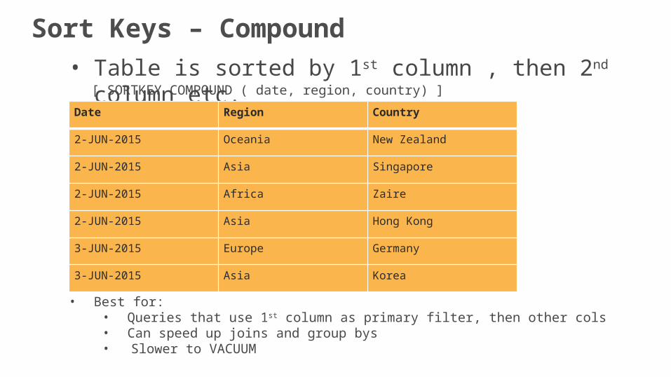
• Table is sorted by 1st column , then 2nd column etc.[ SORTKEY COMPOUND ( date, region, country) ]
• Best for: • Queries that use 1st column as primary filter, then other cols• Can speed up joins and group bys• Slower to VACUUM
Date Region Country
2-JUN-2015 Oceania New Zealand
2-JUN-2015 Asia Singapore
2-JUN-2015 Africa Zaire
2-JUN-2015 Asia Hong Kong
3-JUN-2015 Europe Germany
3-JUN-2015 Asia Korea
Sort Keys – Compound
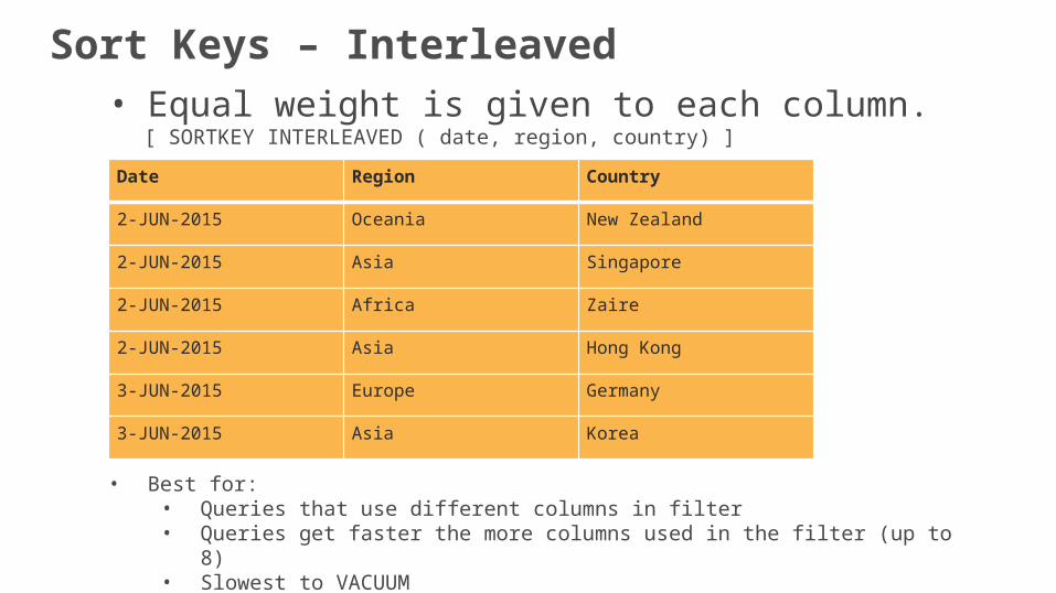
• Equal weight is given to each column.[ SORTKEY INTERLEAVED ( date, region, country) ]
• Best for: • Queries that use different columns in filter• Queries get faster the more columns used in the filter (up to 8)• Slowest to VACUUM
Date Region Country
2-JUN-2015 Oceania New Zealand
2-JUN-2015 Asia Singapore
2-JUN-2015 Africa Zaire
2-JUN-2015 Asia Hong Kong
3-JUN-2015 Europe Germany
3-JUN-2015 Asia Korea
Sort Keys – Interleaved
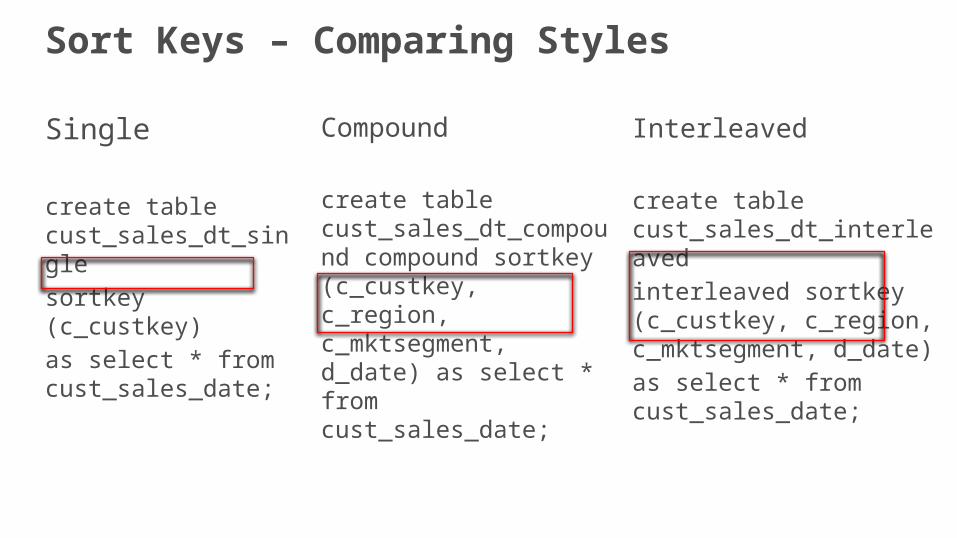
Sort Keys – Comparing Styles
Single
create table cust_sales_dt_single
sortkey (c_custkey)
as select * from cust_sales_date;
Compound
create table cust_sales_dt_compound compound sortkey (c_custkey, c_region, c_mktsegment, d_date) as select * from cust_sales_date;
Interleaved
create table cust_sales_dt_interleaved
interleaved sortkey (c_custkey, c_region, c_mktsegment, d_date)
as select * from cust_sales_date;
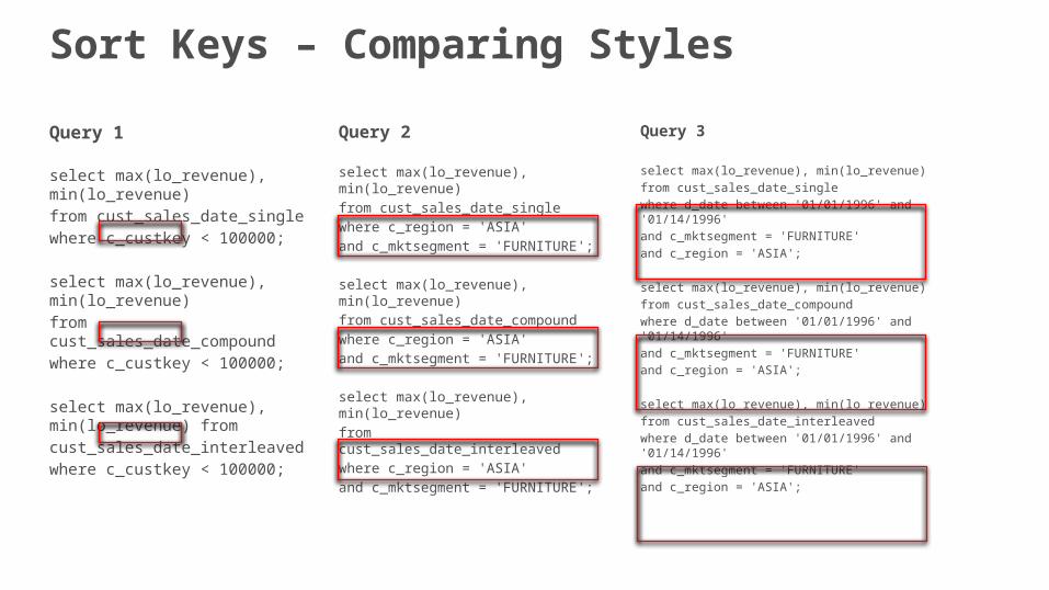
Query 1
select max(lo_revenue), min(lo_revenue)
from cust_sales_date_single
where c_custkey < 100000;
select max(lo_revenue), min(lo_revenue)
from cust_sales_date_compound
where c_custkey < 100000;
select max(lo_revenue), min(lo_revenue) from
cust_sales_date_interleaved
where c_custkey < 100000;
Query 2
select max(lo_revenue), min(lo_revenue)
from cust_sales_date_single
where c_region = 'ASIA'
and c_mktsegment = 'FURNITURE';
select max(lo_revenue), min(lo_revenue)
from cust_sales_date_compound
where c_region = 'ASIA'
and c_mktsegment = 'FURNITURE';
select max(lo_revenue), min(lo_revenue)
from cust_sales_date_interleaved
where c_region = 'ASIA'
and c_mktsegment = 'FURNITURE';
Query 3
select max(lo_revenue), min(lo_revenue)
from cust_sales_date_single
where d_date between '01/01/1996' and '01/14/1996'
and c_mktsegment = 'FURNITURE'
and c_region = 'ASIA';
select max(lo_revenue), min(lo_revenue)
from cust_sales_date_compound
where d_date between '01/01/1996' and '01/14/1996'
and c_mktsegment = 'FURNITURE'
and c_region = 'ASIA';
select max(lo_revenue), min(lo_revenue)
from cust_sales_date_interleaved
where d_date between '01/01/1996' and '01/14/1996'
and c_mktsegment = 'FURNITURE'
and c_region = 'ASIA';
Sort Keys – Comparing Styles
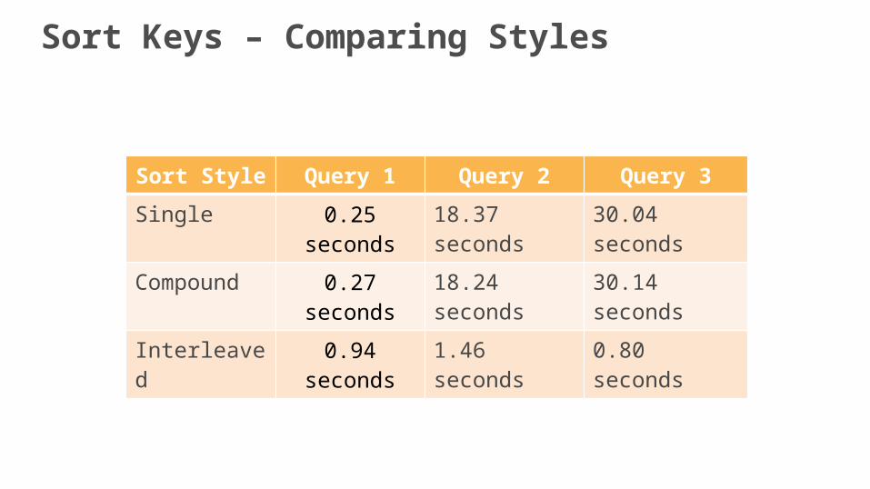
Sort Style Query 1 Query 2 Query 3
Single 0.25 seconds 18.37 seconds 30.04 seconds
Compound 0.27 seconds 18.24 seconds 30.14 seconds
Interleaved 0.94 seconds 1.46 seconds 0.80 seconds
Sort Keys – Comparing Styles
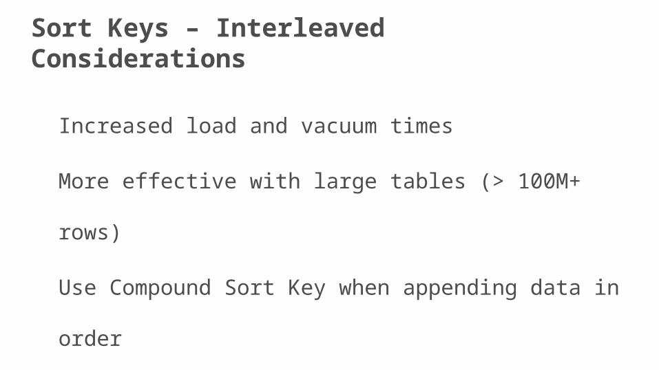
Increased load and vacuum times
More effective with large tables (> 100M+ rows)
Use Compound Sort Key when appending data in order
Sort Keys – Interleaved Considerations
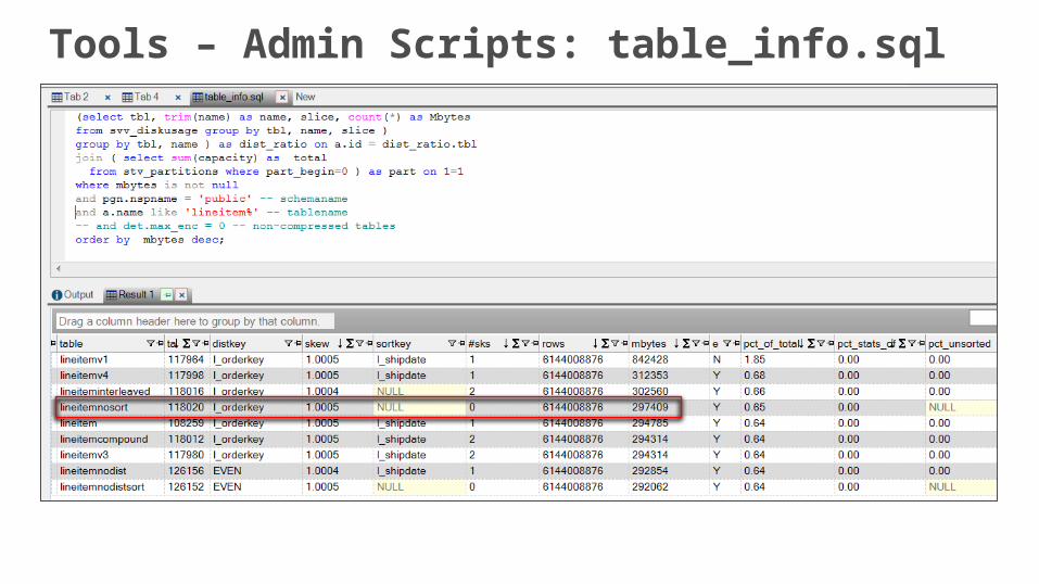
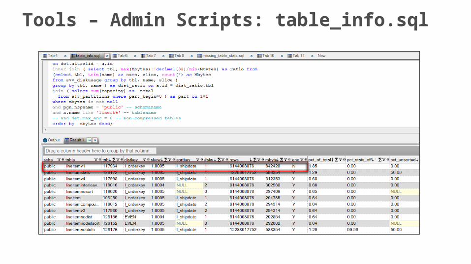
Tools – Admin Scripts: table_info.sql
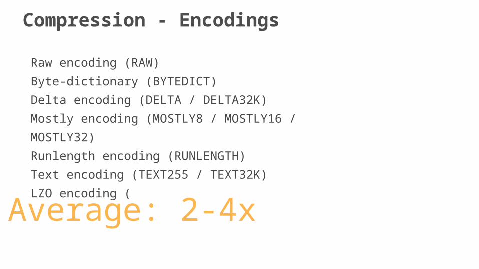
Raw encoding (RAW)
Byte-dictionary (BYTEDICT)
Delta encoding (DELTA / DELTA32K)
Mostly encoding (MOSTLY8 / MOSTLY16 / MOSTLY32)
Runlength encoding (RUNLENGTH)
Text encoding (TEXT255 / TEXT32K)
LZO encoding (
Average: 2-4x
Compression - Encodings
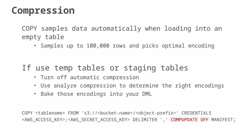
COPY samples data automatically when loading into an empty table• Samples up to 100,000 rows and picks optimal encoding
If use temp tables or staging tables• Turn off automatic compression
• Use analyze compression to determine the right encodings
• Bake those encodings into your DML
COPY <tablename> FROM 's3://<bucket-name>/<object-prefix>' CREDENTIALS <AWS_ACCESS_KEY>;<AWS_SECRET_ACCESS_KEY> DELIMITER ',' COMPUPDATE OFF
MANIFEST;
Compression
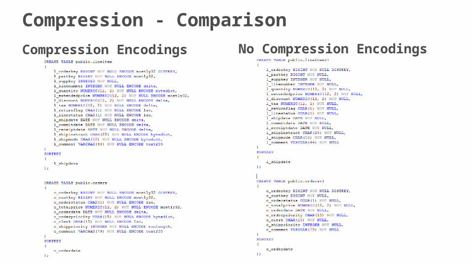
Compression Encodings
Compression - Comparison
No Compression Encodings
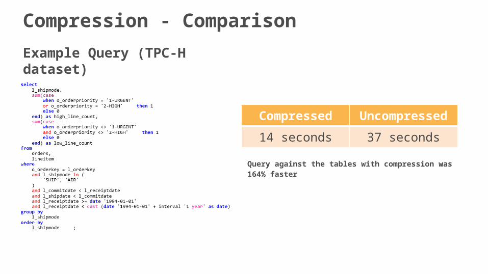
Example Query (TPC-H dataset)
Compressed Uncompressed
14 seconds 37 seconds
Query against the tables with compression was 164% faster
Compression - Comparison
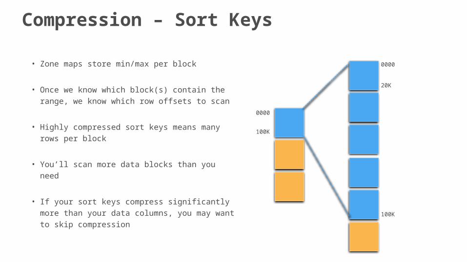
• Zone maps store min/max per block
• Once we know which block(s) contain the range, we know which row offsets to scan
• Highly compressed sort keys means many rows per block
• You’ll scan more data blocks than you need
• If your sort keys compress significantly more than your data columns, you may want to skip compression
0000
100K
0000
100K
20K
Compression – Sort Keys
Tools – Admin Scripts: table_info.sql
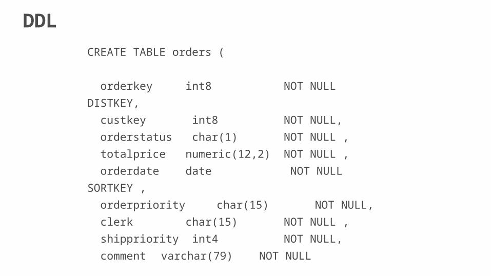
CREATE TABLE orders (
orderkey int8 NOT NULL
DISTKEY,
custkey int8 NOT NULL,
orderstatus char(1) NOT NULL ,
totalprice numeric(12,2) NOT NULL ,
orderdate date NOT NULL
SORTKEY ,
orderpriority char(15) NOT NULL,
clerk char(15) NOT NULL ,
shippriority int4 NOT NULL,
comment varchar(79) NOT NULL
);
DDL
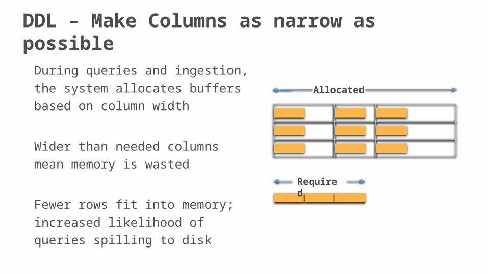
During queries and ingestion, the
system allocates buffers based on
column width
Wider than needed columns mean
memory is wasted
Fewer rows fit into memory;
increased likelihood of queries
spilling to disk
Allocated
Required
DDL – Make Columns as narrow as possible
Define Primary & Foreign Keys
Not Enforced but…..Helps optimizer with query plan
DDL
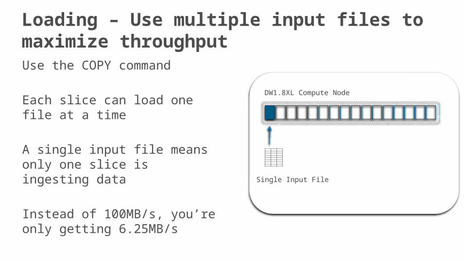
Use the COPY command
Each slice can load one file at a time
A single input file means only one slice is ingesting data
Instead of 100MB/s, you’re only getting 6.25MB/s
DW1.8XL Compute Node
Single Input File
Loading – Use multiple input files to maximize throughput
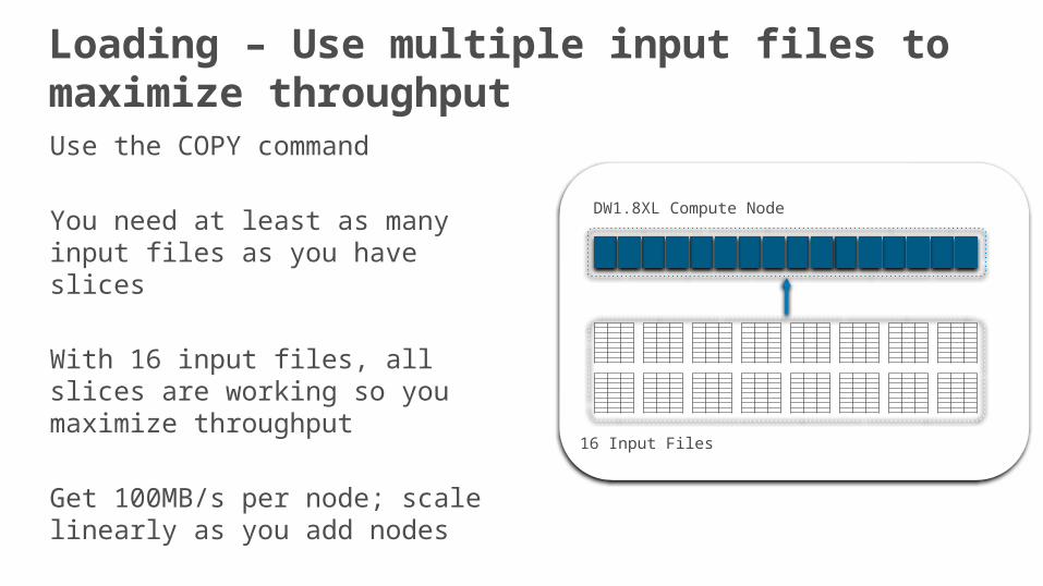
Use the COPY command
You need at least as many input files as you have slices
With 16 input files, all slices are working so you maximize throughput
Get 100MB/s per node; scale linearly as you add nodes
16 Input Files
DW1.8XL Compute Node
Loading – Use multiple input files to maximize throughput
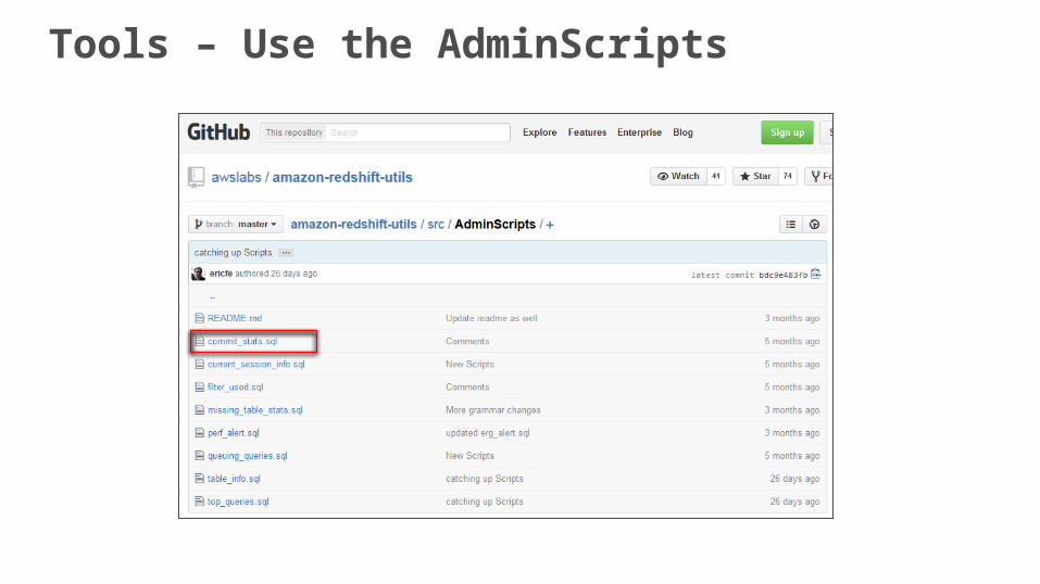
Tools – Use the AdminScripts
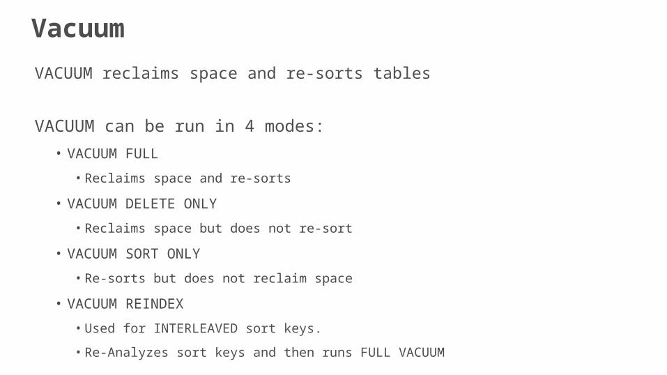
VACUUM reclaims space and re-sorts tables
VACUUM can be run in 4 modes:
• VACUUM FULL
• Reclaims space and re-sorts
• VACUUM DELETE ONLY
• Reclaims space but does not re-sort
• VACUUM SORT ONLY
• Re-sorts but does not reclaim space
• VACUUM REINDEX
• Used for INTERLEAVED sort keys.
• Re-Analyzes sort keys and then runs FULL VACUUM
Vacuum
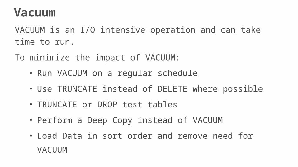
VACUUM is an I/O intensive operation and can take time to run.
To minimize the impact of VACUUM:
• Run VACUUM on a regular schedule
• Use TRUNCATE instead of DELETE where possible
• TRUNCATE or DROP test tables
• Perform a Deep Copy instead of VACUUM
• Load Data in sort order and remove need for VACUUM
Vacuum
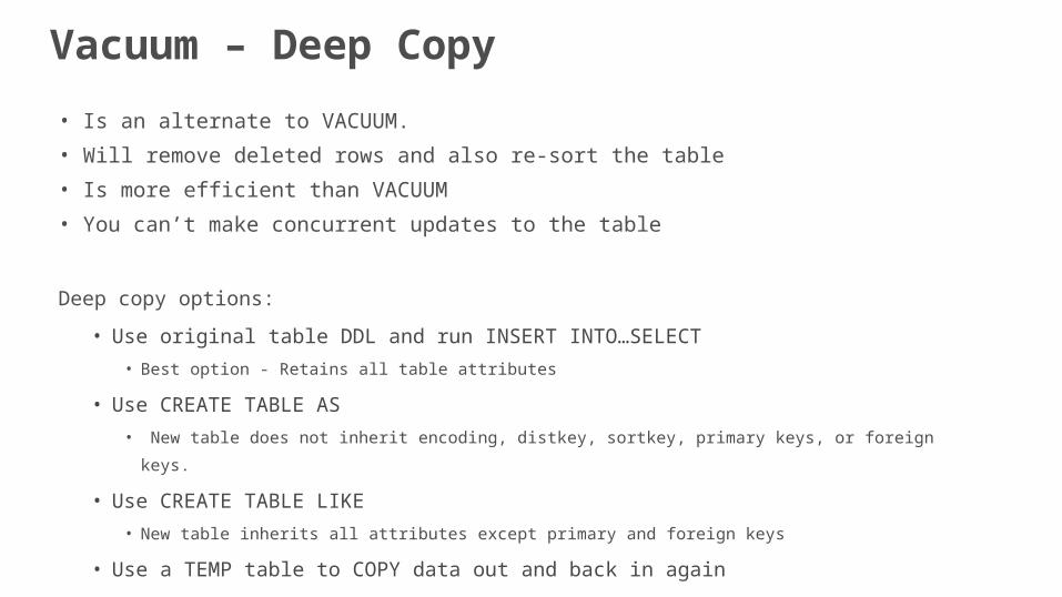
• Is an alternate to VACUUM.
• Will remove deleted rows and also re-sort the table
• Is more efficient than VACUUM
• You can’t make concurrent updates to the table
Deep copy options:
• Use original table DDL and run INSERT INTO…SELECT
• Best option - Retains all table attributes
• Use CREATE TABLE AS
• New table does not inherit encoding, distkey, sortkey, primary keys, or foreign keys.
• Use CREATE TABLE LIKE
• New table inherits all attributes except primary and foreign keys
• Use a TEMP table to COPY data out and back in again
• Retains all attributes but requires two full inserts of the table
Vacuum – Deep Copy
Redshift’s query optimizer relies on up-to-date statistics
Update stats on sort/dist key columns after every load
Analyze
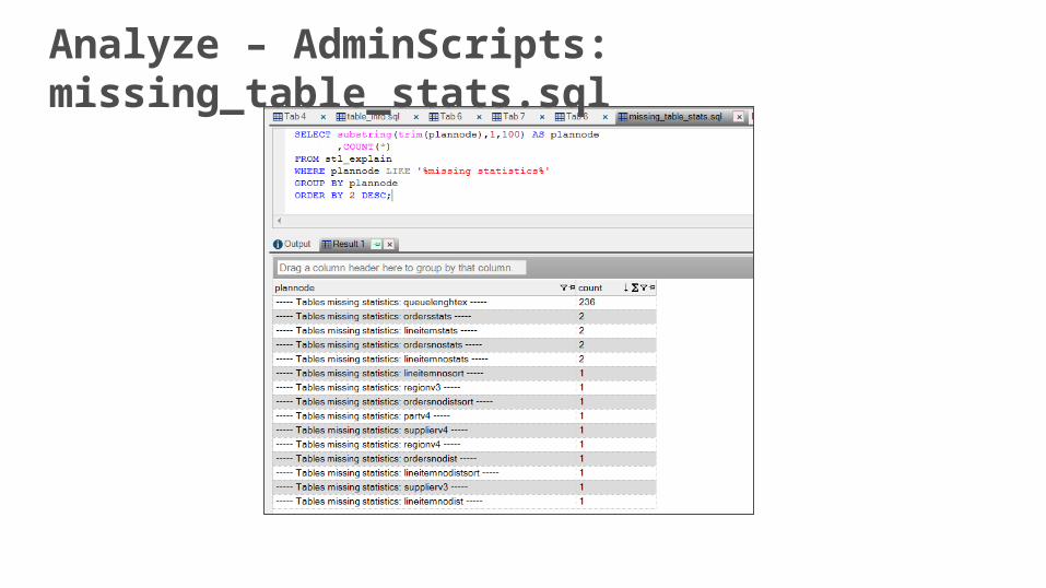
Analyze – AdminScripts: missing_table_stats.sql
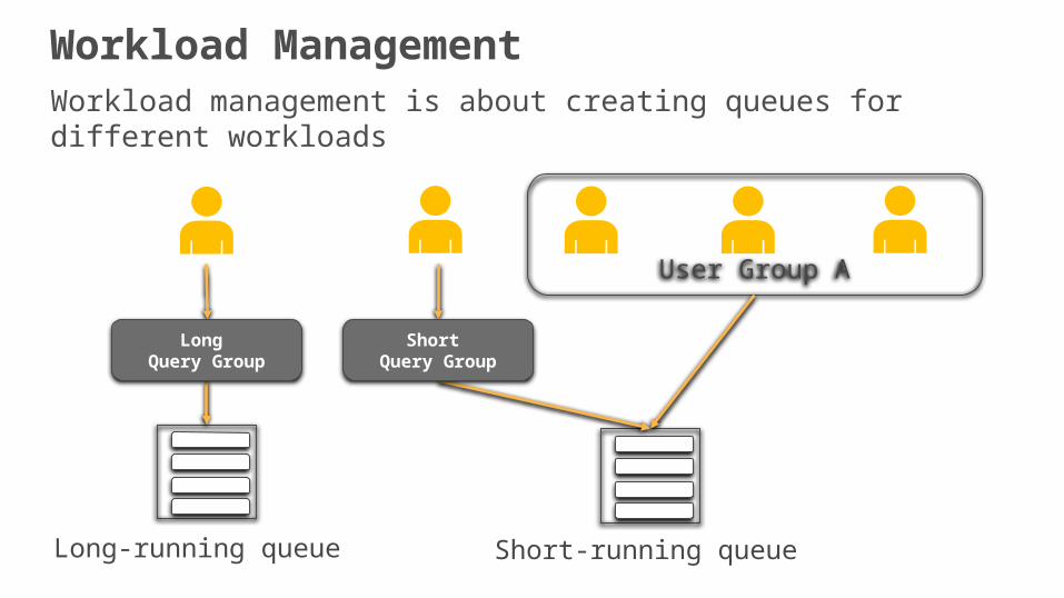
Workload ManagementWorkload management is about creating queues for different workloads
User Group A
Short-running queueLong-running queue
Short Query Group
Long Query Group
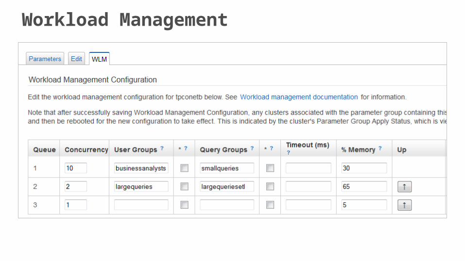
Workload Management
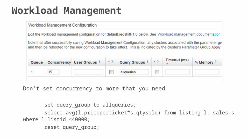
Workload Management
Don’t set concurrency to more that you need
set query_group to allqueries;
select avg(l.priceperticket*s.qtysold) from listing l, sales s where l.listid <40000;
reset query_group;
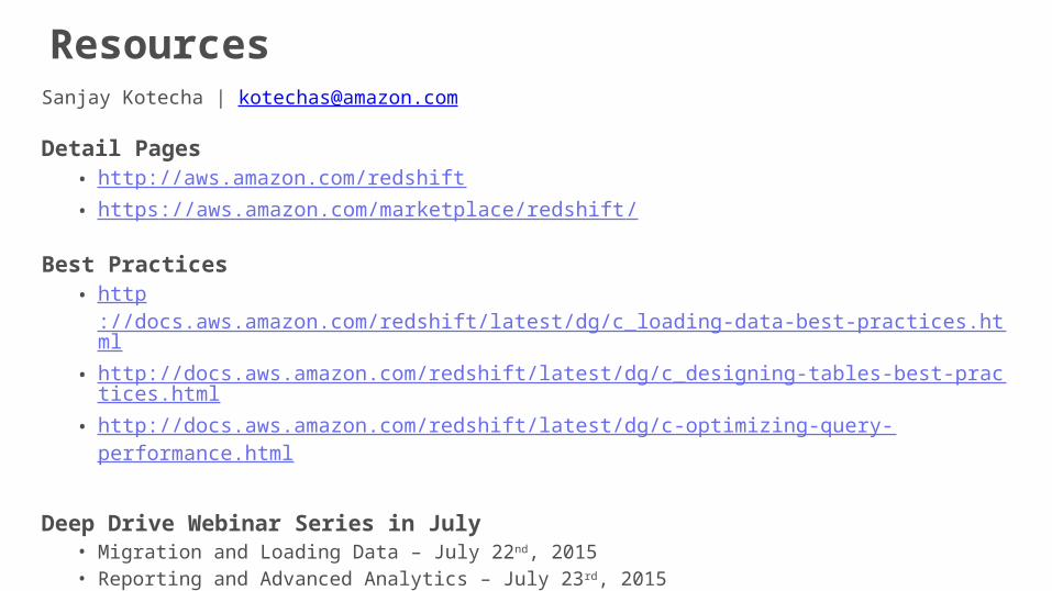
ResourcesSanjay Kotecha | [email protected]
Detail Pages• http://aws.amazon.com/redshift• https://aws.amazon.com/marketplace/redshift/
Best Practices• http://docs.aws.amazon.com/redshift/latest/dg/c_loading-data-best-practices.html• http://docs.aws.amazon.com/redshift/latest/dg/c_designing-tables-best-practices.ht
ml• http://docs.aws.amazon.com/redshift/latest/dg/c-optimizing-query-performance.html
Deep Drive Webinar Series in July• Migration and Loading Data – July 22nd, 2015• Reporting and Advanced Analytics – July 23rd, 2015

Thank you!