average displacement-support vector machines via ...average displacement-support vector machines via...

Average Displacement-Support Vector Machines via Lyapunov Exponents and Wave Approximate Function in Power Load

Forecasting Model

JIANFENG LIa&b, DONGXIAO NIUa, MING WUb, YONGLI WANGa , MENG LIc, MINGYUE YONGd aSchool of Economics and Management,

North China Electric Power University, Beijing, CHINA

bChina Electric Power Research Institute , Beijing, CHINA

cEconomic and Technological Research Institute, State Grid Henan Electric Power Company

CHINA dBeijing Electric Power Corporation,

Beijing, CHINA

Abstract：- With the development and improvement of the electricity market, the role of power load forecasting in competitive market is being recognized. It is very important to ensure the security and stability of electric network by accurate load forecasting. Meanwhile, the reform of the electricity market leads to a result that it is far more difficult for the match between power supply-side and demand-side, which brings new challenges to the power load forecasting industry. According to the chaotic and non-linear characters of power load data, and to prove the effectiveness and accuracy, the model of AD-SVM (average displacement-support vector machines) based on L yapunov exponents and wave approximation function optimization was established. Firstly, the optimal time delay and embedding dimension sequence of time series are determined by average displacement method. Secondly the method of maximum Lyapunov exponents is devoted to selecting the appropriate embedding dimension and time delay, which proves the effectiveness of the accuracy invariants of phase-space; and then considering the volatility autocorrelation characteristics, we determine learning parameters based on the exploiting fluctuation approximation function and embedding dimension, which can greatly assist us with the prediction of future market; meanwhile, article applies KNN method to estimate noise standard deviation so as to determine the parameter selection. Finally, support vector machine is utilized for establishing the model of power load forecasting. In addition, for existing generalized autoregressive heteroscedasticity of phenomenon of LSSVM prediction error, In this paper, the prediction error is modified by GARCH model on the basis of the original and the prediction error of the auto regressive process is eliminated. Therefore, it can further enhance prediction accuracy. In order to prove the rationality of chosen dimension and the effectiveness of the model, any other random dimensions were selected to compare with the calculated dimension while BP algorithm was used to compare with the result of SVM. The results show that the model is effective and more accurate in the forecasting of short-term power load. Keywords: - Power load forecasting; Support vector machines; Lyapunov exponents; average displacement; Wave approximate function; embedding dimension; GARCH error correction

1 Introduction

Power system short-term load forecasting is of great importance to the reliability and economic operation of the power system. Accurate load

forecasting can start and stop the generator set economically and rationally, and maintain the safety and stability of the grid operation. Now to break the monopoly, deregulation, the introduction

WSEAS TRANSACTIONS on POWER SYSTEMS Jianfeng Li, Dongxiao Niu, Ming Wu,

Yongli Wang, Meng Li, Mingyue Yong

E-ISSN: 2224-350X 258 Volume 13, 2018

of competition, China's power industry has established the electricity market power system reform, the purpose is to more rational allocation of resources. And due to the complexity and variability of the electricity market, short-term load forecasting has received more and more attention and attention. How to predict the power load of the power grid accurately and effectively is becoming more and more popular. etc (see 1)

Domestic and foreign scholars have made a lot of research on t he theory and methods of load forecasting, proposing a variety of forecasting methods. Conventional methods for short-term load forecasting have trend extrapolation, regression analysis, time series method, gray prediction, Kalman filtering, expert system method, etc (see [2,3,4]). With the gradually established modern power system management information system and the continuous improvement of the weather forecasting level, it is no longer difficult to accurately obtain all kinds of historical data needed for load forecasting, and the following modern intelligent methods have emerged: wavelet analysis, Artificial neural network method, support vector machine method, data mining method, fuzzy prediction method, optimal combination method. These methods gradually increase the speed and accuracy of load forecasting. In general, the commonly used methods for power load forecasting can be broadly divided into two categories: one is the traditional method represented by time series method, and the other is the new artificial intelligence method represented by artificial neural network. Among them, the artificial neural network method is undoubtedly the most studied and the most widely used short-term load forecasting method in recent years. However, the ANN is not perfect. Since the algorithm itself contains too many heuristic components, there are some inherent and insurmountable defects. For example, it is too dependent on the initial value, the network structure is difficult to determine, and it is likely to converge to a local minimum.

SVM is a m achine learning algorithm proposed in the 90's of last century, the theory is based on statistical learning theory proposed by Vapnik. The SVM regression algorithm has the advantages of short convergence time, high prediction accuracy, less adjustable parameters and easy structure determination, and does not require too much prior information and usage skills, and its generalization ability is much better than that of artificial nerve the internet. It has significant advantages. However, support vector machines

have outstanding advantages, meanwhile, there are also some problems, which are mainly reflected in the following aspects: the selection of the key parameters in SVM has a d irect impact on the generalization performance and prediction results of the prediction model, and the lack of a structured common method The conventional forecasting method uses different means to analyze the power load based on the trend of the known data. However, this is only an approximate mathematical analysis of the load model, and does not essentially analyze the chaos inherent in the power system characteristic.

A method of short-term power load forecasting based on data mining techniques was proposed by Liuxi Zhe, which introduced the SVM method into the short-term load forecasting research area (see [5]). In the literature, the support vector machine method is used to explore the short-term load forecasting of power system (see [6-10]). Based on the characteristics of power load forecasting random sequence growth and nonlinear wave, Niu Dongxiao utilized an approach which can effectively reflect the growth behavior of Markov chains and gray support vector machine, so that power load forecasting accuracy has been greatly improved (see [11]); De Yi Wang established a short term load forecasting model based on chaotic characteristic and least square support vector machine that combined with the theory of phase space reconstruction of chaotic time series and the regression theory of support vector machine on the basis of chaotic characteristics of the load time series with chaotic time series (see [12]), Grant and Jason Lee, etc. who used artificial neural network forecasting method and the combination of chaos theory, designed and developed real-time energy monitoring system to guarantee electricity peak generation capacity when the demand for electricity is at peak (see [13,14]). Li Dongdong and Wang Jianzhou, etc. applied the combination of maximum Lyapunov exponent and fractal interpolation extrapolation algorithm, for urban power load data of actual load of short-term load forecasting, reflecting the superiority and applicability of these two programs (see [15- 20]). The forecast based on RBF neural network forecasting method and Support Vector Machine which leaded into a satisfactory result basing on t he combination and the utilization of artificial memory model and rigorous nonlinear model predictive was utilized by some people like Fan Zhiping (see [21]). Niu Dongxiao and Fang Jun solve large-scale nonlinear



E-ISSN: 2224-350X 259 Volume 13, 2018

regression and time series problems by using support vector machines and Nystrom based on approximation of the least squares (see [22]). A new method was proposed by Zhang Qian to overcome the training set of single support vector machine with the application of neural call function. The results show that this is an effective prediction method (see [23]). Based on the function of the degree of membership function, Xu Yabin improved BP artificial neural network algorithm and simulated test. The results show that the short-term electric load forecasting can achieve a better effect (see [24]). In order to improve the accuracy of power load forecasting, using a continuous ant colony optimization based on support vector machine algorithm model to improve the accuracy and speed of prediction (see [25]).

In order to obtain a better prediction effect and ensure the accuracy, this paper put to use the method of combining the average displacement method and the support vector machine based on the Lyapunov index and the wave approximation. Firstly, phase space reconstruction is performed on power load time series. Then, phase points in reconstructed phase space are used as su pport vector machines Feature input training on t he model, so as to find the optimal parameter values, to achieve automatic optimization of the parameters selected. At the same time, the value of learning parameters is determined by the method of wave approximation function analysis. The Lyapunov exponent is an important index to describe the chaotic properties of dynamical systems. Whether a system has chaotic properties can be determined by whether its Lyapunov exponent has positive or not. This method not only considers the chaotic characteristics of the power system, but also overcomes the defects that the traditional parameter selection method relies mainly on empirical calculations and low efficiency. In addition, in the end, the paper also uses GARCH model to eliminate and correct the prediction error, and eliminates the autoregressive process of the prediction error based on the original, which has good fitting and predictive ability

2 Chaotic time series and lyapunov exponents

According to the chaos theory, the driving factors of the chaotic system are mutually influential, and thus the data points generated in

time are also related. At present, the analysis of sequence kinetic factors, widely used is the delayed coordinate state space reconstruction method. In general, the phase space of a system may be very high, even infinite, but in most cases the number of dimensions is not known. In fact, the phase space delay coordinate reconstruction method can expand the given time series to 1, 2 1, , , ,n nx x x x− three-dimensional and even higher dimensional space and the information which exposed sufficiently from time series can be classified and extracted.

2.1. Reconstruction of phase space. The technology of reconstruction phase space

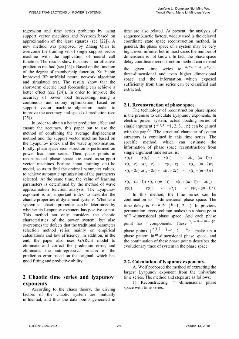
is the premise to calculate Lyapunov exponents. In electric power system, actual loading series of single argument { ( )jx t =1, 2, 3… n} can be gained with the gap t∆ . The structural character of system attractors is contained in this time series. The specific method, which can estimate the information of phase space reconstruction from single argument time series, is:

1( )x t 2( )x t ( )jx t ( ( 1) )nx t m τ− −

1( )x t τ+ 2( )x t τ+ ( )jx t τ+ ( ( 2) )nx t m τ− −

1( 2 )x t τ+ 2( 2 )x t τ+ ( 2 )jx t τ+ ( ( 3) )nx t m τ− −

1( ( 1))x t m+ − 2( ( 1))x t m+ − ( ( 1))jx t m+ − ( )nx t

1( )y t 2( )y t ( )jy t ( ( 1) )ny t m τ− − In this method, the time series can be

continuation to m -dimensional phase space. The time delay is τ = k t∆ ( k =1, 2….). In previous permutation, every column makes up a phase point of m -dimensional phase space. And each phase

point has m components. These ( 1)pn n m τ= − −

phase points { ( )jx t , j =1, 2… pn } make up a phase pattern in m -dimensional phase space, and the continuation of these phase points describes the evolutionary trace of system in the phase space.

2.2. Calculation of lyapunov exponents. A. Wolf proposed the method of extracting the

largest Lyapunov exponent from the univariate time series. The method and steps are as follows:

1) Reconstructing m -dimensional phase space with time series.



E-ISSN: 2224-350X 260 Volume 13, 2018

2) Choosing minimal τ which marks the correlation among each phase space coordinates by average displacement method.

3) In the continuation m -dimensional phase space, the initial phase point 1( )A t is chosen as a reference point. There are m components in the phase space, they

are 1 1 1 1( ), ( ), ( 2 ), ( ( 1))x t x t x t x t mτ τ+ + + − . According to the following formula:

nbt i jL Min Y Y = − i j≠ (1)

1( )B t is the nearest neighborhood point

to 1( )A t can be impetrated. nbtL Which is assumed 1( )L t means the distance between 1( )A t and its nearest neighborhood point in Euclidean meaning. Suppose 2 1t t k t= + ∆ with k△t as the step

length and 2( )A t evolves into 2( )A t , meanwhile 1( )B t evolves into 2( )B t , then the distance 2 2 2( ) ( ) ( )A t B t l t= is got.

Let 1λ represent the rate of exponential growth

and2

2 1( ) ( )2l t L t λ= , then the following equation can be got.

1 2 1 2 2 11/ ( ) log ( ( ) / ( ))k t t l t L tλ = − ( 1)t∆ = (2)

λ is the Lyapunov exponent. It can take

advantage of λ to judge the stability of time behavior of the system.

4) Search a small neighborhood point 2( )C t which subjects to the angle 1θ in the nearest neighborhood points to 2( )A t (If it can’t meet the two conditions: small 1 1θ and neighborhood, it should still choose 1( )B t ). Suppose 3 2t t k t= + ∆ , 2( )A t evolves into 3( )A t and 2( )C t evolves into 3 3 3( ) ( ) ( )C t A t l t= and 2 2 2( ) ( ) ( )A t C t L t= , then:

2 2 1 2 3 21/ ( ) log ( ( ) / ( ))k t t l t L tλ = − (3)

It cannot stop carrying out the previous steps

until it reaches the end of

point-group{ }( ), 1, 2, ,j pX t j n= . Then, choose the average of the calculated rates of exponential

growth as t he maximal estimated value of Lyapunov exponent. That is

1 2( 1)

( )( ) 1/ log

( )i

i

l tLE m N

L t −

= (4)

/pN n k= means total steps of step length.

5) In order to increase the embedding dimension, repeat the above steps (3) ~ (4) until the estimated value of the index is in balance. Then get the maximum Lyapunov exponent value at this moment.

3 SVM regression theory For the training sample set, as the input

variable value is the corresponding output value, the basic idea of support vector machine regression theory is to find a nonlinear mapping from input space to output space. Through this nonlinear mapping, the data is mapped to a High-dimensional feature space, and linear regression in the feature space using the following estimated function, in the form:

[ ]( ) ( )f x x bω φ= ⋅ +

m:φ →R F ,ω∈F (5)

b is the threshold value. The problem of the function approximate is equivalent with the minimizing the following problem:

[ ] [ ] 2 2

1( )

s

reg emp ii

f f eλ ω λ ω=

= + = +∑R R C (6)

{ }( ) max 0, ( )y f x y f xε

ε− = − − (7)

[ ]reg fR is objective function and s is the

number of the sample. ie is loss function and λ

is adjusting constant meter. 2ω reflects

f complexity in the high-dimensional flat space. The following loss function can be gained concerning with the rarefaction character of the linear insensitive loss function ε .

{ }( ) max 0, ( )y f x y f x

εε− = − − (8)

Empirical risk function is



E-ISSN: 2224-350X 261 Volume 13, 2018

[ ]1

1 ( )n

empi

f y f xn

εε

=

= −∑R (9)

According to statistic theory, the regression

function is determined by minimizing the following functions:

( )21min2 i iω ξ ξ∗ + +

∑

n

i=1C (10)

( )(i iy x bω φ ε ξ ∗− ⋅ − ≤ + (11) ( )( ), i ix b yω φ ε ξ+ − ≤ + (12)

, 0i iξ ξ ∗ ≥ (13)

C is used to balance the model's complex and training error terms, and the relaxation factor, is a loss-insensitive function. This problem translates into the following duality problem:

( )( ), 1

1max[ ( , )2

n

i i j j i ji j

a a a a K X X∗ ∗

=

− − − +∑

( ) ( )1

]l n

i i i ii i

a y a yε ε∗

=

− − −∑ ∑ (14)

1 1

n n

i ii i

a a∗

= =

=∑ ∑ (15)

0 ia∗≤ ≤ C (16) 0 ia≤ ≤ C (17)

Solve the problem, and then the regression

equation is:

( )1

( ) ( , )n

i i ii

f x a a k X X b∗

=

= − +∑ (18)

4 Support vector machine parameter optimization and research the results of correction model.

SVM regression algorithm has the advantages of short convergence time, high prediction accuracy, less adjustable parameters and less structural risk in power load forecasting. It does not require too much prior information and skills, and has better generalization ability. However, support vector machine has outstanding advantages at the same time; there are also some problems, focused on the following aspects:

1) The choice of parameters has great influence on the accuracy of load forecasting. In support vector machine, the selection of several key parameters directly affects the generalization

performance and prediction results of the prediction model, but at present, there is not a unified model in the world, and there is still a lack of structured general method to realize the optimal choice of parameters. Owing to the complexity of the SVM model, adopting a precise method to optimize become an inevitable requirement.

2) A more accurate prediction model can all produce prediction errors because of neglect of secondary influencing factors or other reasons. The so-called prediction error is the difference between the predicted value and the true value. The general prediction model only considers the main influencing factors of load changes, ignoring the secondary influencing factors. Prediction error may form a certain trend under the long-term effect of these secondary factors. Error correction is just a secondary factor that takes these loads into account. A process of fitting the error trend is to combine the advantages of different models and finally increase Prediction of the accuracy of the process.

In response to these problems, we use GARCH model to predict and correct the error after SVM prediction.

4.1. Average displacement method to determine the time delay τ .

The average displacement method with an average delay of displacement vectors to characterize the degree of expansion of phase space, which is the origin of the name of the algorithm. Specifically defined as:

( ) ( )∑ ∑=

−

=+ −=

M

i

m

iijim xx

MS

1

1

1

21ττ (19)

Type: ( )τ1−−= mNM and N are the

sequence length. jzix + and ix are independent coordinates for phase space reconstruction. Let

0mm = the τ derivative, when ( ) 0=τmdS , the τ for the corresponding embedding dimension under the optimal delay time. That the average displacement method, the time delay is the most

appropriate when the slope of the curve ( )τmS dropped to 40% of the initial value for the first time.



E-ISSN: 2224-350X 262 Volume 13, 2018

4.2. Determination of chaotic time series and embedding dimension.

The Lyapunov exponent is used to characterize the average rate of divergence between neighboring points in a system. A positive Lyapunov exponent measures the average exponential decoupling between two adjacent orbits and a negative Lyapunov exponent measures the average of two adjacent orbits. If the index is close to the index, if a discrete nonlinear system is dissipative, a relatively stable positive Lyapunov exponent can be obtained. Therefore, it is determined that the time series is a chaotic time series.

According to the characteristics of chaotic time series, Lyapunov exponent method is used to calculate the corresponding relationship between embedded dimension and Lyapunov exponent (realized by programming software Visual Basic Version 6.0.with.SP6) according to the sample, and the Lyapunov exponent value The floating dimension tends to be stable when the value of the dimension, the embedded dimension is the key data we request, according to the value of time series with the characteristics of the model to establish.

4.3. Determine learning parameters by wave approximate function.

Determine the dimensions n of the sample by the method of Lyapunov index, so Points on t he n-dimensional spaces is:

2

2 22( , ) exp( ) (2 )

2n n

ni n

iR R

x xk x x dx dx π σ

σ−

= − =∫ ∫ (20)

Considering function like(18) ， then the

equation is

*

1( ) ( , ) 0

n

N

i i iiR

k x x dxα α=

− =∑∫ (21)

Formula (21) shows that the mean of the first

term of formula (20) is approximately zero, which represents the fluctuation of the function; item 2 b is approximately a function of the mean value. And taking into account:

2

22( , ) exp( ) 1

2i

i

x xk x x

σ−

= − ≤ (22) *

i iC Cα α− ≤ − ≤ ( 1, 2, )i N= (23)

So that is

*

1( ) ( , )

N

i i i SVi

k x x C nα α=

− ≤ •∑ (24)

{ }( ) max 0, ( )y f x y f xε

ε− = − − (25)

SVn is number of support vectors. The following function can be gained

{ }

1max i y SVi N

y C nµ≤ ≤

− ≤ • (26)

yµ is sample mean of output variables, that is:

1

1 N

y ii

yN

µ=

= ∑ (27)

So the following function can be gained

{ }1

1 max i yi NSV

y Cn

µ≤ ≤

− ≤ (28)

Taking into account the power load as

approximately normally distributed random variables in general, it is recommended to take this article

3

ySV

Cn

σ= (29)

yσ is the difference between the sample

standard variable y , that is

2

1

1 ( )1

N

y i yi

yN

σ µ=

= −− ∑ (30)

4.4. Determine variable ε by KNN.

According to statistical learning theory, variable ε should be proportional to the noise level in the sample, the following formula is:

ln( )3 N

Nε γ= (31)

γ is noise standard deviation; N is sample

size. In the case of unknown γ , method of KNN is used to estimate noise of data.

1/52

21/5

1

1 ( )1

N

i i

ky y

NkN

Nγ∧ ∧

= −−

∑ (32)

/pN n k= means total steps of step length.



E-ISSN: 2224-350X 263 Volume 13, 2018

Among them, iy∧

is iy estimate; k is the

number of nearest neighbors, where k influence γ∧

relatively small.

4.5. GARCH error correction model analysis.

Most statistical methods in econometrics are models for averaging mean values of random variables. The goal of time series analysis is often to predict the future value of the variable. ARCH (autoregressive conditional heteroskedasticity) and GARCH (generalized autoregressive conditional heteroskedasticity) models are designed to describe and predict the variance of dependent variables. Among them, the variance of the explanatory variables depends on the formulation of the formula depending on the past value of the variable, or on some independent exogenous variables.

The GARCH (1,1) model assumes that the variance depends on its hysteresis () and the residual squared hysteresis ().These include 3 simple items as follows.

t t ty x ε= + (33)

2 2 21t t t jδ ω αε βδ− −= + + (34)

Formula (33) is called the mean equation;

formula (34) is called the GARCH equation. GARCH model, called generalized ARCH

model, is an extension of ARCH model, which is developed by Bollerslev (1986). GARCH (P, q) is expressed as follows:

2 2 2

11 1

q p

t i t j t ji j

δ ω α ε β δ− −= =

= + +∑ ∑ (35)

Where P is the maximum lag order GARCH

term, q i s the maximum lag order ARCH term. When all the terms of the GARCH (P, q) model are equal to 0, the GARCH (P, q) model is turned into a pure ARCH (q) model.

4.6. Optimization of support vector machine prediction process based on lyapunov exponent and wave approximate function.

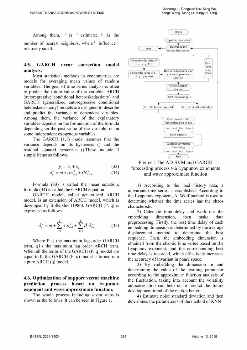
The whole process including seven steps is shown as the follows. It can be seen in Figure 1.

Input the data seties

Determine the series chotic or not

Determine the series of τ、m by AD Deter

mine ε by KNN

Choose kernel function

SVM forecasting

Error analysis

N + 1th forecasting load N + 1th actual load value

Determine N + 1th forecasting error or not

GARCH correction forecasting

Error meet the object

Choose the value of τ、m by Lyapunov

Due to m,determine c,σ2

by wave approximate function

N

Begin

stop N

Y Y

Stop

Error meet the object

N

Figure 1.The AD-SVM and GARCH forecasting process via Lyapunov exponents

and wave approximate function

1) According to the load history data, a univariate time series is established. According to the Lyapunov exponent, A. Wolf method is used to determine whether the time series has the chaos characteristic.

2) Calculate time delay and work out the embedding dimension, then make data preprocessing. Firstly, the best time delay of each embedding dimension is determined by the average displacement method to determine the best sequence. Then, the embedding dimension is obtained from the chaotic time series based on the Lyapunov exponent, and the corresponding best time delay is recorded, which effectively increases the accuracy of invariant in phase space.

3) By embedding the dimension m and determining the value of the learning parameter according to the approximate function analysis of the fluctuation, taking into account the volatility autocorrelation can help us to predict the future development trend of the market better.

4) Estimate noise standard deviation and then determines the parameters ε of the method of KNN



E-ISSN: 2224-350X 264 Volume 13, 2018

5) Parameters in SVM model should be

initialized. iα*iα and b are assigned random values.

6) The training samples are used to establish the objective function of the form (9) ~ (12), then the values of the sum and b a re obtained by converting (9) ~ (12) into (13) ~ (16) using the duality problem. Substitute the obtained parameter values into Eq. (17), use the test sample to calculate the forecast value at a ce rtain time on the N + 1 day, and compare the measured load to determine whether the forecast error meets the standard. If not, go back to the first step to judge the chaos Sex, re-forecast.

7) The GARCH error correction model is used to verify the relative prediction error of the established prediction model, and the relative error prediction value is obtained, finally the corrected error is obtained.

5 Empirical analysis 5.1. Sample selection.

Using the method mentioned in this paper, the short-term load forecasting of power grid in a certain area in Inner Mongolia is studied. The following method proposed in this paper, the regional power grid load forecasting empirical analysis. A total of 8784 data of the grid from 0:00 on January 1, 2013 to 12:00 on June 1, 2014 were selected as test samples and simulated.

According to the characteristics of historical electric load data, the data is processed and the average displacement method is introduced. Through the graph to find the embedded dimension m, the relationship between the delay time τ. As the embedding dimension () increases, the relationship between the two can be drawn. When the slope of the curve changes to 40% of the initial value, the optimal delay time under the embedding dimension is as shown in the following figure.

50

100

150

200

250

4 168 12 20

m=3m=6m=9m=12m=14

Figure 2. AD method to determine the

optimum τ

Table 1.embedding dimension m the best correspondence between the delay time τ

m τ m τ

3 14 9 7

4 12 10 6

5 10 11 4

6 9 12 2

7 8 13 1

8 8 14 1

5.2. Characteristics of chaos.

According to the related theory of chaotic time series, using the A. Wolf method in calculating Lyapunov exponents, the embedding dimension m is calculated by software. The relationship between time delay and Lyapunov exponent is shown in Table 2. According to 4.2 theory, when = 12, When the value of the index begins to be stable and> 0, we can determine that the sequence has the chaotic property; thus we can conclude that the embedding dimension = 12. Use these parameters to reconstruct the phase space.

5.3. Support vector machine prediction. The sample data are normalized and predicted

by using SVM. The calculation tool adopts Libsvm toolbox and kernel function uses radial basis function. From the chaotic time series obtained embedding dimension = 12, select the parameters C = 79.31, = 0.012, = 4.28. In order to compare the influence of embedding dimensions on the prediction results, other dimensions are selected to construct the model for prediction. C = 73.01, = 0.017, = 2.13 when = 11; C = 26.30, = 0.006, = 1.60 when = 14. The results are shown in Table 3.

Using BP neural network calculation, using sigmoid arithmetic function, the number of input layer nodes is 11, the number of output layer nodes is 1, the number of intermediate layer nodes is 8 based on experience, the system accuracy is set as 0.001, and the maximum number of iterations is 5000 times. The results of the two methods are shown in Table 3.

5.4. Predicted values and evaluating indicator.



E-ISSN: 2224-350X 265 Volume 13, 2018

Predicted Values and Evaluating Indicator Relative error and root-mean-square relative error are used as the final evaluating indicators:

100%t tr

t

x yE

x−

= × (36)

21

tr

nt t

t ntr t

x yRMSRE

N n x=

−= −

∑ (37)

Table 2.Corresponding relationship between embedding dimension and Lyapunov index

value embedded

dimension m best time delay τ

Lyapunov exponent

3 14 1.93960346334233E-02 4 12 1.91412341819302E-02 5 10 1.85346290486013E-02 6 9 1.73296039103426E-02 7 8 1.62926254213395E-02 8 8 1.55855695367583E-02 9 7 1.43411411714047E-02 10 6 1.40034692507806E-02 11 4 1.37648343297765E-02 12 2 1.37579437635724E-02 13 2 1.37917989114717E-02 14 1 1.36936856261568E-02

Table 3.The comparison of each method to predict the results

Time point

Actual load

Er SVM(12)

relative error(%

Er SVM(11)

relative error(%)

Er SVM(13)

relative error(%)

Er BP(12)

relative error(%)

00：00 1220.679 1190.063 -2.51 1181.789 -3.19 1182.943 -3.09 1148.953 -5.88 02：00 1010.763 1030.063 1.91 1045.895 3.48 1042.743 3.16 1048.958 3.78 04：00 910.693 890.067 -2.26 871.785 -4.27 882.7437 -3.07 882.538 -3.09 06：00 980.765 950.063 -3.13 942.864 -3.86 982.647 0.19 948.953 -3.24 08：00 1210.596 1189.067 -1.78 1171.885 -3.20 1172.654 -3.13 1158.578 -4.30 10：00 1586.667 1574.358 -0.79 1556.157 -1.92 1549.452 -2.34 1557.767 1.82 12：00 1616.630 1607.348 -0.58 1680.507 3.95 1646.841 1.87 1672.537 3.46 14：00 1187.326 1216.399 2.45 1236.063 4.10 1229.651 3.56 1223.264 3.03 16：00 1298.681 1293.996 -0.36 1284.448 -1.09 1317.504 1.45 1298.870 0.01 18：00 2033.626 2005.428 -1.38 1989.988 -2.15 2026.371 -0.36 2006.313 -1.34 20：00 2045.348 2059.617 0.70 1983.735 -3.01 2052.219 0.34 2038.675 -0.33 22：00 1686.667 1674.358 -0.73 1656.157 -1.81 1649.452 -2.21 1657.767 -1.71 RMSRE 0.0171 0.0310 0.0246 0.0319

From the above calculation results can be

seen: 1) In order to verify the scientificity of the

Lyapunov exponent selection embedding dimension, the two cases of less than 12 dimensions and more than 12 dimensions are respectively selected to be compared with the prediction results of the 12-dimensional support vector machine algorithm. The relative error of prediction results was no more than 3%. The number of qualified points was 11 at 12 dimensions, 4 at 11 dimensions and 7 at 13

dimensions. Based on the relative root mean square error of prediction results, The relative root mean square error is less than the values of other dimensions, so the prediction results in 12-dimensional are better than those in other dimensions.

2) Comparison between Prediction Results Based on Support Vector Machine and BP Neural Network. The relative error of support vector machine (MVVM) prediction result is not large, the maximum error is 3.13%, and the difference



E-ISSN: 2224-350X 266 Volume 13, 2018

between maximum error and minimum error is 5.58%. However, the amplitude of BP neural network error is very large with the maximum error of 5.88% the difference in error is 9.66%. The relative error of the prediction results was not more than 3%, and the number of support vector machines was 11, a nd BP neural network was 5. Based on the root mean square relative error of the prediction results, the support vector machine is less than the root mean square error of BP neural network. As can be seen from the above comparison, when the embedding dimension is determined, the prediction effect of SVM is better than that of BP neural network.

5.5. Short term load forecasting based on GARCH error correction.

1) Error analysis. The stability of the time series is the premise

of the GARCH model. Therefore, the data source should be first tested for stationarity. The simplest test method is to calculate the autocorrelation function and the partial correlation function.

The first-order autocorrelation and partial-correlation functions with a lag 10 a re calculated for the fitted relative error sequence e at 12:00 at the power load prediction of AD-SVM based on Lyapunov exponent and fluctuation approximation function. The results are shown in Table 4. AC stands for autocorrelation function and PAC stands for partial correlation function.

Table 4.Error sequence autocorrelation and partial correlation test results

AC PAC Q-Stat Prob

1 0.465 0.465 11.260 0.000

2 0.356 0.202 16.780 0.001 3 0.234 0.054 20.372 0.000 4 0.161 0.069 24.893 0.000 5 0.033 -0.247 24.782 0.000 6 -0.131 -0.210 24.356 0.000 7 -0.168 -0.188 26.369 0.001 8 -0.192 -0.086 28.476 0.000 9 -0.234 -0.043 30.568 0.001

10 -0.256 -0.068 33.043 0.001

As can be seen from Figure 1, the autocorrelation coefficient of the sequence can quickly fall into the random area, which can be initially judged that the sequence is stable. In order to increase the reliability of judgment, a more rigorous extension of the Augmented Dicky-Fuller Test (ADF) is used. ADF test for the first order differential sequence, the results in Table 3`

Table 5.ADF test fitting relative error

ADF-Statistics Prob.* Significance level (threshold)

-28.472834 0.0049 (1%) -3.562428

(%5) -2.896375 (%5) -2.584723

It can be seen that ADF = -28.4, less than all

the cutoffs of significance levels of 1%, 5%, and 10%, and P = 0.0049, approximately equal to 0, indicating that there is no unit root in the sequence and the relative error sequence is stationary.

2) GARCH model prediction error The article establishes model through

LIBSVM and GARCH Toolbox and MATLAB of GA. Model Evaluation error using relative error (RE, referred to as IRE) said:

%100ˆ

×−

=i

iiRE y

yyI

Wherein iy is the predicted value? After repeated tests, ar (1) was selected as the

mean equation regression, and ARMA (1, 1) was found to have the best fitting result.

The GARCH error correction model is established to correct the error of 12 points in one day, the prediction error and the corrected error, as shown in Table 6. As can be seen from the table before the forecast average relative error is not corrected to 0.0171, 1.71%, has been in line with the standards, show that the predictive model is appropriate, after a GARCH error correction, the average prediction relative error of 0.0126, 1.26%, improve the accuracy of the 0.45 percentage points, prediction model is more reasonable.



E-ISSN: 2224-350X 267 Volume 13, 2018

Table 6.Forecast and correction results (unit: million kilowatts (%)

Sample

Actual load

Er SVM(12)M

relative error

Corrected error

00：00 1220.679 1190.063 -2.51 -1.23

02：00 1010.763 1030.063 1.91 0.82

04：00 910.693 890.067 -2.26 1.97

06：00 980.765 950.063 -3.13 -2.23

08：00 1210.596 1189.067 -1.78 -0.89

10：00 1586.667 1574.358 -0.79 1.37 12：00 1616.630 1607.348 -0.58 -0.78 14：00 1187.326 1216.399 2.45 1.56 16：00 1298.681 1293.996 -0.36 0.67 18：00 2033.626 2005.428 -1.38 1.35 20：00 2045.348 2059.617 0.70 0.21 22：00 1686.667 1674.358 -0.73 -0.45 RMSE 0.0171 0.0126

From Table 3 and Table 6 to establish various

types of prediction error contrast analysis chart, you can visually see the error range changes, shown in Figure 3.

0 2 4 6 8 10 12-0.06

-0.04

-0.02

0

0.02

0.04

0.06

Time point

rela

tive

erro

r

Er SVM(11)Er SVM(12)Er SVM(13)Er SVM(12)MEr BP(12)

Figure 3. Comparison of various types of

prediction error analysis chart

Through 11, 12, 13 dimensional SVM prediction model and 12 dimensional BP prediction model error and correction model error analysis can be seen: The prediction error of the 12-dimensional SVM model is the smallest, and the distribution of points is close to zero. The absolute value of the

relative error is no more than 2%, that is to say, the predicted value is closer to the actual load; the prediction error of 12-dimensional SVM model is second, and the absolute value of relative error is no more than 3%. The errors of 11-dimensional, 13-dimensional SVM and 12-dimensional BP neural network are larger and the prediction errors are scattered. It can be seen that the model obtained by GARCH after the 12-dimensional SVM prediction model has a higher fitting degree

In order to verify the prediction accuracy and stability of the GARCH error correction prediction model, the daily load of 24 points in the future is forecasted. As shown in Figure 5, it can be seen that the daily forecast achieves a high accuracy within the predicted seven days and the forecast error is controlled within 3.0%, which fully demonstrates that using GARCH error correction model for power load forecasting has a higher stability.

GARCH model was used to model the error correction of the other 24 points, to give surface plots fitting error after correction:

05

1015

2025

02

4

68

-0.03

-0.02

-0.01

0

0.01

0.02

0.03

hourdate

rela

tive

erro

r

Figure 4. GARCH fitting error correction

surface plot

It can be seen that the range of variation of fitting error after correction is between [-0.03, 0.03]. Compared with the pre-correction error, the error sequence is smoother. It shows that the GARCH error correction model has good effect on eliminating the autoregression of prediction error.

6 Conclusion After the actual data verification, it is proved

that this method has a good effect in short-term



E-ISSN: 2224-350X 268 Volume 13, 2018

load forecasting, and the following conclusions are obtained:

1) The power load data show apparent chaotic character. Chaotic time series is established and chaotic parameters are computed by A.Wolf, then SVM prediction model is established to make prediction. After verification of the actual data, it is proved that this method has a g ood effect in short-term load forecasting.

2）There is a set of appropriate embedding dimension and time delay, which makes SVM predict the short-term load to achieve higher accuracy. The optimal time delay of each embedding dimension is determined by means of the average displacement method, and then select the number of embedding dimension using the method of Lyapunov exponents of making λ begin to level off, writing down the optimal delay time, and the predicted results with chosen dimension and other random dimension are compared. The results show that there is a su itable embedding dimension which is used to predict the power load effectively.

3) When the embedding dimension is the same, the prediction accuracy of support vector machine is far greater than that of BP neural network. The reason is that the BP neural network has the least empirical risk, the computation is easy to fall into the local optimum, the support vector machine based on the structural risk is the smallest, the local optimum is the global optimum, and thus has better generalization ability than the BP neural network.

4) The generalized autoregressive heteroskedasticity of the least square support vector machine prediction error is eliminated and corrected. Stripping part of the influencing factors, it is effectively improving the prediction accuracy. Through the real example verification, the prediction error of the SVM power load forecasting model optimized by the GARCH model modified Lyapunov exponent and the fluctuation approximation function has better fitting and forecasting ability.

In the actual forecasting, because the data such as weather and temperature are difficult to obtain and the load data is relatively easy to obtain, we can use this method to carry on s hort-term load forecasting, which has strong practical significance.

References

[1] Dongxiao Niu, Shuhua Cao, and Yue Zhao, Technology and Application of Power Load Forecasting, Beijing: China Power Press, 1998.

[2] Wang Hui-zhong, Zhou Jia, LiuKe.Summary of Research on t he Short-term Load Forecasting Method of the Electric Power System. Electrical Automation,37(1)(2015)36-38

[3] Zhou Chao. Summarization on Load Forecasting Method of Electrical Power System. Power Supply Corporation,(2012)32-39

[4] Wang Ji-cheng. Research on Chaos Forecast Methods of Load of Electrical Power System. Applied Technology, 2013.pp.75-76

[5] Liu xi-zhe. Study of the Distributed Power System Load Forecasting Based on Choas Theory (D). Changsha University, 2011.

[6] Zhao D F, Wang M, Zhang J S, et al. A support vector machine approach for short term load forecasting [J]. Proceedings of the Csee, 22(4)(2002)26-29

[7] Yuan-Cheng L I, Fang T J, Er-Keng Y U. Study of support vector machines for short-term load forecasting. Proceedings of the Csee. Proceedings of the Csee, 2003.pp.654-659.

[8] Wang Bao-cheng. A Predict on Power Load in A Short Term Based on SVR. Times Agricultural Machinery,42(5)(2015)51-52

[9] Qiu Cun-yong, Xiao Jian. Power System Short-Term Load Forecasting Based on Support Vector Regression. Computer Simulation,30(11) (2013)62-64

[10] Wang Y J, Dian-Wen L I. Research on the Short-Term Load Forecast Based on t he Improved SVM. Electrical Measurement & Instrumentation, 51(18)(2014)1-4

[11] Niu D, Lv J L, Zhang X. The Improved Markov Error Correcting Method in Gray SVM for Power Load Forecasting// International Symposium on Intelligent Information Technology Application Workshops. IEEE Computer Society, 2008.pp.793-796.

[12] Wang De-yi,Yang Zhuo, Yang Guo-qing. Short-Term Load Forecasting Based on Chaotic Characteristic of Loads and Least Squares Support Vector Machines. Power System Technology, 32(7)(2008)66-69.

[13] Grant, Jason Lee. Short-term peak demand forecasting using an artificial neural network with controlled peak demand through



E-ISSN: 2224-350X 269 Volume 13, 2018

intelligent electrical loading. University of Miami, (2014)632-635.

[14] Quan H, Srinivasan D, Khosravi A. Short-term load and wind power forecasting using neural network-based prediction intervals. IEEE Transactions on Neural Networks & Learning Systems, 25(2)(2014)303-315.

[15] Wang J, Jia R, Zhao W, et al. Application of the largest Lyapunov exponent and non-linear fractal extrapolation algorithm to short-term load forecasting. Chaos Solitons & Fractals, 45(s 9–10) (2012)1277-1287.

[16] Liu kui. Research on short-term load forecasting method based on c haos and wavelet neural network. Southwest Jiaotong University Master Degree Thesis, 2012.

[17] Wang J, Zhou J, Bing P. A hybrid neural genetic method for load forecasting based on phase space reconstruction. Kybernetes the International Journal of Systems & Cybernetics, 39(8)(2010)1291-1297.

[18] Wang J, Jia R, Zhao W, et al. Application of the largest Lyapunov exponent and non-linear fractal extrapolation algorithm to short-term load forecasting. Chaos Solitons & Fractals, 45(s 9–10) (2012)1277-1287.

[19] Li Dongdong, Qin Zishan. Short-term Load Forecasting for Microgrid Based on Method of Chaotic Time Series. Proceedings of the CSU-EPSA, 27(5)(2015)14-17.

[20] Li Lan-you,Du Jie, Shao Ding-hong, LU Jin-gui. Larges Lyapunov exponent of short-term electric load forecasting model simulation. Computer Engineering and Design, 28(12)(2007)5934-5938.

[21] Fan Z, Qin Z, Hong T, et al. The studying of combined power-load forecasting by error evaluation standard based on RBF network and SVM method// Control and Decision Conference, CCDC '09. Chinese. 2009.pp.4016-4019.

[22] Wu J, Niu D. Short-Term Power Load Forecasting Using Least Squares Support Vector Machines(LS-SVM)// Computer Science and Engineering,2009. WCSE '09.Second International Workshop on. IEEE, 2009.pp.246-250.

[23] Zhang Q. Application of Support Vector Machine and Fuzzy Rules Method for Power Load Forecasting// International Conference on Computer Engineering & Applications. IEEE Computer Society, 2010.pp.542-545.

[24] Xu Y, Du P. Researching about Short-Term Power Load Forecasting Based on Improved

BP ANN Algorithm// icise. IEEE Computer Society,2009.pp.4094-4097.

[25] Sun W, Zhao W. Mid-long term power load forecasting based on MG-CACO and SVM method// Future Computer and Communication (ICFCC), 2010 2nd International Conference on. IEEE, 2010.pp.V1-118-V1-121.

[26] Quan Wen, Yangchuan Zhang, and Shijie Chen, “The analysis approach based on chaotic time series for load forecasting,” Power System Technology, 2001.pp.13-16.

[27] Zhishan Liang, Liming Wang, and Dapeng Fu, “Short-term power load forecasting based on lyapunov exponents,” Proceeding of the CSEE,1998.pp.368-472.

[28] Francis E. H. Tay, Lijuan Cao. Application of Support Vector Machines in Financial Time Series Forecasting. The International Journal of Management Science, 2001.pp.309-317.

[29] Kodba Stane, Perc Matjaz, Marhl Marko. Detecting chaos from a t ime series. European Journal of Physics 26(1) (2005)205-215.

[30] Wolf A, Swift J B and Swinney H L. Determining lyapunov exponents from a time series. Physics D, 1985.pp.285-317.

[31] Liu Qiming, Jiamalihan·Kumashi, Hua Dong, Li Pengfei. Load Forecasting Based on Support Vector Machine Analysis. Electric technology, 2013.pp.34-36

[32] Zhang Xuegong. Nature of Statistical Learning Theory. Beijing tsinghua university press , 2000.

[33] Zhang L, Liu X S, Yin H J. Application of support vector machines based on t ime sequence in power system load forecasting. Power System Technology, 28(19)(2004)38-41.

[34] .Li Xin. Study on pow er load forecasting model based on phase space reconstruction and SVM. Electrical Measurement ＆Instrumentation, 51(24)(2014)6-8

[35] Dongning Tan and Donghan Tan, “Small-sample machine learning theory-statistical learning theory,” Journal of Nanjing University of Science and Technology,25(1)(2001)108-112.

[36] Zhou You, Xiang Jinglin. A Quickly Converging and Numerically Stable Method of Calculating Finite Time Lyapunov Exponents (FTLEs) of Multidimensional System with Degenerate Spectrum. Journal of



E-ISSN: 2224-350X 270 Volume 13, 2018

Northwestern Poly technical University. 23(2)(2005)240-243.

[37] Huo Ming. Research on Parameters Optimization of SVM Model for Short-term Loading Forecasting. Hunan University, 2009.



E-ISSN: 2224-350X 271 Volume 13, 2018

average displacement-support vector machines via ...average displacement-support vector machines via...

Documents