ave extraction in numerical relativity - uni … · wave extraction in numerical relativity...
TRANSCRIPT
Doctoral Dissertation
Wave Extraction in Numerical Relativity
Dissertation zur Erlangung des
naturwissenschaftlichen Doktorgrades
der Bayrischen Julius-Maximilians-Universitat Wurzburg
vorgelegt von
Oliver Elbracht
aus Warendorf
Institut fur Theoretische Physik und Astrophysik
Fakultat fur Physik und Astronomie
Julius-Maximilians-Universitat Wurzburg
Wurzburg, August 2009
Eingereicht am: 27. August 2009
bei der Fakultat fur Physik und Astronomie
1. Gutachter: Prof. Dr. Karl Mannheim
2. Gutachter: Prof. Dr. Thomas Trefzger
3. Gutachter: -
der Dissertation.
1. Prufer: Prof. Dr. Karl Mannheim
2. Prufer: Prof. Dr. Thomas Trefzger
3. Prufer: Prof. Dr. Thorsten Ohl
im Promotionskolloquium.
Tag des Promotionskolloquiums: 26. November 2009
Doktorurkunde ausgehandigt am:
Gewidmet meinen Eltern, Gertrud und Peter, fur all ihre Liebe und
Unterstutzung.
To my parents Gertrud and Peter, for all their love, encouragement and
support.

Wave Extraction in Numerical Relativity
Abstract This work focuses on a fundamental problem in modern numerical rela-
tivity: Extracting gravitational waves in a coordinate and gauge independent way to
nourish a unique and physically meaningful expression.
We adopt a new procedure to extract the physically relevant quantities from the
numerically evolved space-time. We introduce a general canonical form for the Weyl
scalars in terms of fundamental space-time invariants, and demonstrate how this ap-
proach supersedes the explicit definition of a particular null tetrad.
As a second objective, we further characterize a particular sub-class of tetrads in
the Newman-Penrose formalism: the transverse frames. We establish a new connection
between the two major frames for wave extraction: namely the Gram-Schmidt frame,
and the quasi-Kinnersley frame. Finally, we study how the expressions for the Weyl
scalars depend on the tetrad we choose, in a space-time containing distorted black
holes. We apply our newly developed method and demonstrate the advantage of our
approach, compared with methods commonly used in numerical relativity.
Abriss Diese Arbeit konzentriert sich auf eine fundamentale Problematik der nu-
merischen Relativitatstheorie: Die Extraktion von Gravitationswellen in einer eich-
und koordinateninvarianten Formulierung, um ein physikalisch interpretierbares Ob-
jekt zu erhalten.
Es wird eine neue Methodik entwickelt, um die physikalisch relevanten Großen aus
einer numerisch erzeugten Raumzeit zu extrahieren. Wir prasentieren eine allgemein-
gultige kanonische Formulierung der Weyl Skalare im Newman-Penrose Formalismus
v

als eine Funktion von fundamentalen Raumzeit-Invarianten. Dadurch zeigt sich, dass
mit Hilfe dieser Methodik die explizite Konstruktion eines Vierbeins vollstandig re-
dundant ist.
Als weiteren Schwerpunkt charakterisieren wir innerhalb des Newman-Penrose
Formalismus eine spezielle Untergruppe von Tetraden, die transversen Frames. Es wird
eine bisher unbekannte Verbindung zwischen den primar genutzen Vierbeinen fur
die Extraktion der Wellenform abgeleitet, dem Gram-Schmidt Vierbein und dem quasi-
Kinnersley Vierbein. Abschliessend studieren wir die Abhangigkeit der Gravitations-
wellen eines gestorten Schwarzen Loches vom verwendeten Vierbein. Wir berechnen
die Form der Gravitationswellen in dieser Raumzeit und demonstrieren inwieweit
unsere neue Methodik robustere und exaktere Ergebnisse liefert, als die gewohnlich
verwendeten Ansatze zur Extraktion des Signals.
vi
Wave Extraction in Numerical Relativity
Full list of publications by the author
This thesis is mainly based upon the following publications:
• Nerozzi, Andrea; Elbracht, Oliver - Using curvature invariants for wave extrac-
tion in numerical relativity, accepted by Physical Review D (2009).
• Elbracht, Oliver; Nerozzi, Andrea - Using curvature invariants for wave extrac-
tion in numerical relativity. II. Wave extraction in distorted black hole space-
times, submitted to Physical Review D.
• Elbracht, Oliver; Nerozzi, Andrea - A new approach to wave extraction in nu-
merical relativity, submitted to Journal of Physics: Conference Series (refereed).
Other publications by the author:
• Elbracht, Oliver; Nerozzi, Andrea; Matzner, Richard - Wave extraction in nu-
merical evolutions of distorted black holes, oclc/66137068 (2005).
• Burkart, Thomas; Elbracht, Oliver; Spanier, Felix - Simulation results of our
newly developed PIC codes, AN, Vol.328, Issue 7 (unrefereed).
• Rodig, Constanze; Burkart, Thomas; Elbracht, Oliver; Spanier, Felix - Multi-
wavelength periodicity study of Markarian 501, Astronomy and Astrophysics, Vol-
ume 501, Issue 3, 2009, pp.925-932.
vii
• Burkart, Thomas; Elbracht, Oliver; Ganse, Urs; Spanier, Felix - The influence
of the mass-ratio on the acceleration of particles by lamentation instabilities,
submitted to The Astrophysical Journal.
The work has been supported through a research scholarship from the Elitenetz-
werk Bayern (Elite Network of Bavaria). The work contained in this thesis is in part
done within the International Research Training Group (GRK 1147/1) funded by the
Deutsche Forschungsgesellschaft (DFG).
Doctoral Dissertation
Author: Oliver Elbracht
email address: [email protected]
viii
Contents
1. Introduction 1
1.1. Notation and Units . . . . . . . . . . . . . . . . . . . . . . . . . . . . . . . 5
2. The 3+1 Split and Initial Data 9
2.1. Initial Value Problem . . . . . . . . . . . . . . . . . . . . . . . . . . . . . . 9
2.2. The 3+1 Decomposition - Separating Space from Time . . . . . . . . . . 12
2.3. The ADM Formalism . . . . . . . . . . . . . . . . . . . . . . . . . . . . . 12
2.4. BSSN - An Alternative . . . . . . . . . . . . . . . . . . . . . . . . . . . . . 16
3. Gravitational Waves 21
3.1. The Linearized Theory of Gravity . . . . . . . . . . . . . . . . . . . . . . 21
3.2. A Wave Solution and the Transverse-Traceless Gauge . . . . . . . . . . . 26
3.2.1. Interaction of Gravitational Waves with Test-Particles . . . . . . . 28
3.2.2. Polarization of a Plane Wave . . . . . . . . . . . . . . . . . . . . . 30
3.3. Interaction of Gravitational Waves with Detectors . . . . . . . . . . . . . 33
3.4. The Energy of Gravitational Radiation . . . . . . . . . . . . . . . . . . . . 37
3.5. Gravitational Waves from Perturbed Black Holes . . . . . . . . . . . . . . 38
3.5.1. Perturbation Theory and Quasi-Normal Modes . . . . . . . . . . 38
3.5.2. The Regge-Wheeler and Zerilli Equation . . . . . . . . . . . . . . 40
4. The Newman-Penrose Formalism 47
4.1. Mathematical Preliminaries . . . . . . . . . . . . . . . . . . . . . . . . . . 48
4.1.1. Directional Derivatives and Ricci Rotation Coefficients . . . . . . 50
4.1.2. The Commutation Relation and Structure Constants . . . . . . . 51
4.1.3. The Ricci Identities . . . . . . . . . . . . . . . . . . . . . . . . . . . 51
ix
Contents
4.1.4. The Bianchi Identities . . . . . . . . . . . . . . . . . . . . . . . . . 52
4.2. Null Tetrads and Null Frames . . . . . . . . . . . . . . . . . . . . . . . . . 53
4.3. Spin Coefficients . . . . . . . . . . . . . . . . . . . . . . . . . . . . . . . . 55
4.4. Weyl Tensor and Weyl Scalars . . . . . . . . . . . . . . . . . . . . . . . . . 56
4.5. Curvature Invariants . . . . . . . . . . . . . . . . . . . . . . . . . . . . . . 58
4.6. Tetrad Transformations . . . . . . . . . . . . . . . . . . . . . . . . . . . . . 59
4.6.1. Type I Rotations . . . . . . . . . . . . . . . . . . . . . . . . . . . . 60
4.6.2. Type II Rotations . . . . . . . . . . . . . . . . . . . . . . . . . . . . 61
4.6.3. Type III Rotations . . . . . . . . . . . . . . . . . . . . . . . . . . . . 62
4.7. Petrov Classification . . . . . . . . . . . . . . . . . . . . . . . . . . . . . . 63
4.8. Physical Interpretation of the Weyl Scalars & Peeling-off Theorem . . . 65
4.8.1. Petrov Type N . . . . . . . . . . . . . . . . . . . . . . . . . . . . . . 67
4.8.2. Petrov Type III . . . . . . . . . . . . . . . . . . . . . . . . . . . . . 67
4.8.3. Petrov Type D . . . . . . . . . . . . . . . . . . . . . . . . . . . . . . 68
4.8.4. Petrov Type II . . . . . . . . . . . . . . . . . . . . . . . . . . . . . . 68
4.8.5. Petrov Type I . . . . . . . . . . . . . . . . . . . . . . . . . . . . . . 69
4.9. Goldberg-Sachs Theorem . . . . . . . . . . . . . . . . . . . . . . . . . . . 69
4.10. Bondi Frame . . . . . . . . . . . . . . . . . . . . . . . . . . . . . . . . . . . 70
4.11. Kinnersley Tetrad . . . . . . . . . . . . . . . . . . . . . . . . . . . . . . . . 72
4.12. Black Hole Space-Times in the NP Formalism . . . . . . . . . . . . . . . 73
4.13. Perturbation Approach in the NP Formalism . . . . . . . . . . . . . . . . 74
4.13.1. The Perturbation Equations . . . . . . . . . . . . . . . . . . . . . . 74
4.13.2. Teukolsky Master equation . . . . . . . . . . . . . . . . . . . . . . 75
4.13.3. Asymptotic Behavior . . . . . . . . . . . . . . . . . . . . . . . . . . 77
4.14. An Energy Measurement . . . . . . . . . . . . . . . . . . . . . . . . . . . 78
4.15. Selecting the Proper Frame for Wave Extraction . . . . . . . . . . . . . . 79
4.15.1. Transverse Frames & Quasi-Kinnersley Frame . . . . . . . . . . . 80
4.15.2. Finding the Quasi-Kinnersley Frame . . . . . . . . . . . . . . . . 81
5. Non-Perturbative Approach for Wave Extraction 87
5.1. A new Formalism for Wave Extraction . . . . . . . . . . . . . . . . . . . . 88
x
Contents
5.2. Redefining the Weyl Scalars in Transverse Frames . . . . . . . . . . . . . 89
5.3. The Bianchi Identities . . . . . . . . . . . . . . . . . . . . . . . . . . . . . 91
5.4. The Ricci Identities . . . . . . . . . . . . . . . . . . . . . . . . . . . . . . . 92
5.5. Directional Derivatives . . . . . . . . . . . . . . . . . . . . . . . . . . . . . 94
5.6. The Type D Spin Relation . . . . . . . . . . . . . . . . . . . . . . . . . . . 96
5.7. Spin Coefficients as Directional Derivatives . . . . . . . . . . . . . . . . . 99
5.8. The Function H . . . . . . . . . . . . . . . . . . . . . . . . . . . . . . . . 101
5.9. Weyl Scalars in Terms of Curvature Invariants . . . . . . . . . . . . . . . 103
5.9.1. Final Expressions for the Weyl Scalars and Peeling Behavior . . . 105
5.9.2. Conclusion . . . . . . . . . . . . . . . . . . . . . . . . . . . . . . . 107
6. Distorted Black Hole Space-Times in the NP Formalism 109
6.1. Brill Wave Initial Data . . . . . . . . . . . . . . . . . . . . . . . . . . . . . 110
6.1.1. Pure Gravitational Waves . . . . . . . . . . . . . . . . . . . . . . . 110
6.1.2. Distorted Black Hole Initial Data . . . . . . . . . . . . . . . . . . . 113
6.2. Weyl Scalars and Spin Coefficients on the Initial Slice . . . . . . . . . . . 114
6.3. Finding the Transverse Frames . . . . . . . . . . . . . . . . . . . . . . . . 118
6.3.1. The First Transverse Frame . . . . . . . . . . . . . . . . . . . . . . 118
6.3.2. The Quasi-Kinnersley Frame . . . . . . . . . . . . . . . . . . . . . 122
6.4. Connecting the Tetrads in Type D . . . . . . . . . . . . . . . . . . . . . . 126
6.5. Spin-Boost Degree of Freedom . . . . . . . . . . . . . . . . . . . . . . . . 128
6.6. Perturbation Theory for the Close Limit . . . . . . . . . . . . . . . . . . . 132
6.6.1. Perturbed NP Quantities in the Gram-Schmidt Tetrad . . . . . . 135
6.6.2. Perturbed NP Quantities in the Symmetric Tetrad . . . . . . . . . 137
6.6.3. Boost to the Kinnersley Tetrad . . . . . . . . . . . . . . . . . . . . 138
6.7. Extracting the Signal at Future Null Infinity . . . . . . . . . . . . . . . . 139
6.8. Limitations and Possible Issues of the Gram-Schmidt Approach . . . . . 141
6.8.1. Case I - Pseudo-Spherical Coordinates . . . . . . . . . . . . . . . 142
6.8.2. Case II - Transformation r→ rg(t) . . . . . . . . . . . . . . . . . . 144
7. Conclusion and Outlook 147
xi
Contents
A. A1: Evolution Equations 151
A.1. The Evolution Equation for the Metric γµν . . . . . . . . . . . . . . . . . 153
A.2. The Evolution Equation for the Extrinsic Curvature Kµν . . . . . . . . . 153
A.3. The Momentum Constraint . . . . . . . . . . . . . . . . . . . . . . . . . . 155
A.4. The Hamiltonian Constraint . . . . . . . . . . . . . . . . . . . . . . . . . . 156
B. A2: Weyl Scalars in 3+1 Form 157
C. A3: Spin-Weighted Spherical Harmonic Decomposition 165
C.1. Definition and Properties of Spin-weighted Spherical Harmonics . . . . 167
C.2. Decomposition on the Sphere . . . . . . . . . . . . . . . . . . . . . . . . . 169
C.3. Group Properties . . . . . . . . . . . . . . . . . . . . . . . . . . . . . . . . 169
C.4. Explicit Derivation . . . . . . . . . . . . . . . . . . . . . . . . . . . . . . . 170
xii
List of Figures
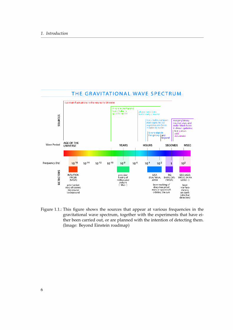
1.1. This figure shows the sources that appear at various frequencies in the
gravitational wave spectrum, together with the experiments that have
either been carried out, or are planned with the intention of detecting
them. (Image: Beyond Einstein roadmap) . . . . . . . . . . . . . . . . . . 6
2.1. The figure illustrates the notion of light cones in general relativity. The
future light cone is the boundary of the causal future of a point in the
hypersurface, and the past light cone is the boundary of its causal past. 11
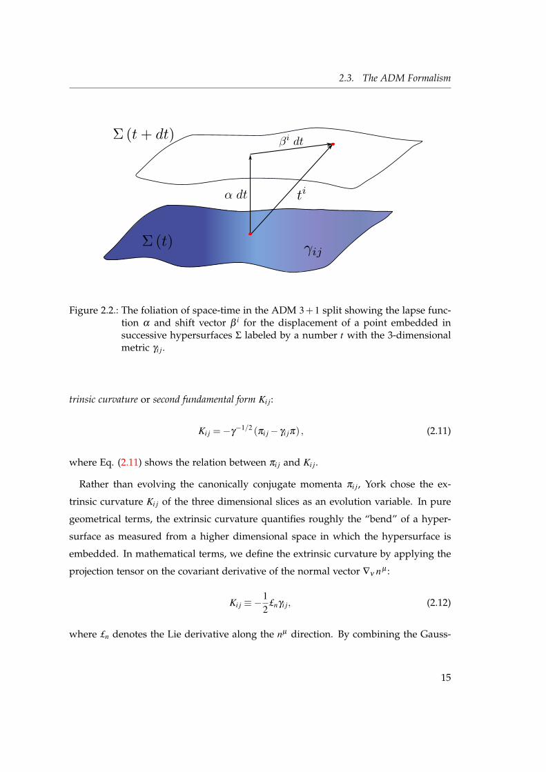
2.2. The foliation of space-time in the ADM 3 + 1 split showing the lapse
function α and shift vector β i for the displacement of a point embed-
ded in successive hypersurfaces Σ labeled by a number t with the 3-
dimensional metric γi j. . . . . . . . . . . . . . . . . . . . . . . . . . . . . . 15
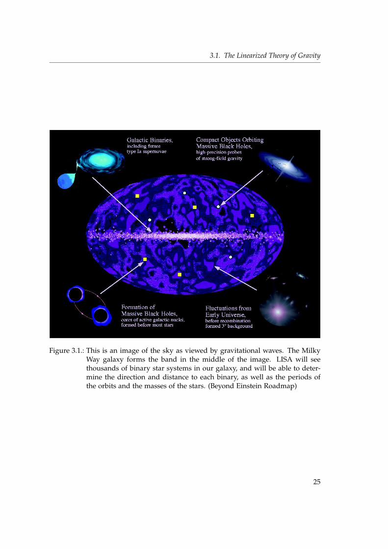
3.1. This is an image of the sky as viewed by gravitational waves. The Milky
Way galaxy forms the band in the middle of the image. LISA will see
thousands of binary star systems in our galaxy, and will be able to de-
termine the direction and distance to each binary, as well as the periods
of the orbits and the masses of the stars. (Beyond Einstein Roadmap) . 25
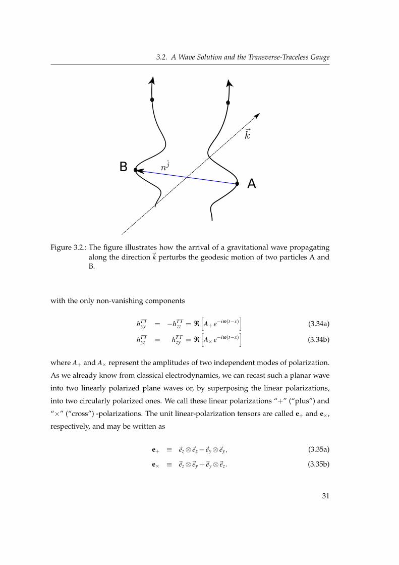
3.2. The figure illustrates how the arrival of a gravitational wave propagat-
ing along the direction~k perturbs the geodesic motion of two particles
A and B. . . . . . . . . . . . . . . . . . . . . . . . . . . . . . . . . . . . . . 31
xiii
List of Figures
3.3. The polarizations of a gravitational wave are illustrated by displaying
their effect on a ring of particles arrayed in a plane perpendicular to
the direction of the wave. The figure shows the distortions the wave
produces if it carries plus/cross polarization or circular polarization,
respectively. . . . . . . . . . . . . . . . . . . . . . . . . . . . . . . . . . . . 32
3.4. This is an artist’s impression showing the basic setup of the LISA space-
craft (Credit: ESA-C. Vijoux). . . . . . . . . . . . . . . . . . . . . . . . . . 34
3.5. An aerial view of the gravitational wave detector GEO600. In the bottom
left corner the central building for the laser and the vacuum tanks can
be seen. The tubes, 600m in length, run in covered trenches at the
edge of the field upwards and to the right. Buildings for the mirrors
are situated at the end of each tube (Credit: AEI Hannover/Deutsche
Luftbild Hamburg). . . . . . . . . . . . . . . . . . . . . . . . . . . . . . . . 36
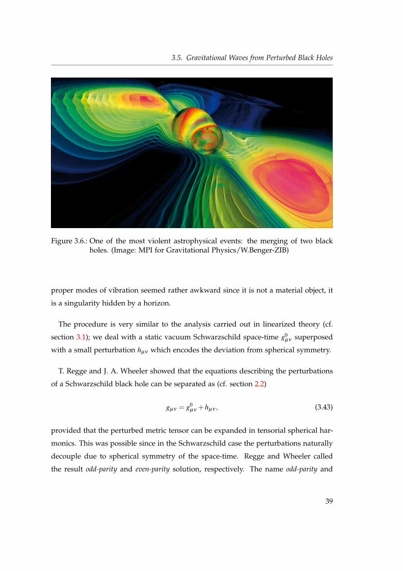
3.6. One of the most violent astrophysical events: the merging of two black
holes. (Image: MPI for Gravitational Physics/W.Benger-ZIB) . . . . . . 39
3.7. The figure shows the strain sensitivity of LIGO and LISA, respectively.
Regions where various sources are predicted to be are also shown. (Im-
age: Beyond Einstein Roadmap) . . . . . . . . . . . . . . . . . . . . . . . 44
4.1. A schematic classification of the different Petrov types suggested by R.
Penrose. The arrows point in the direction of increasing specialization. 64
4.2. The peeling-off theorem. . . . . . . . . . . . . . . . . . . . . . . . . . . . . 66
4.3. A schematic classification of the different Petrov types. . . . . . . . . . . 69
4.4. Illustrating the idea of Bondi coordinates at future null infinity. . . . . . 71
4.5. (a) A transverse frame which is also a quasi-Kinnersley frame: in the
limit of Petrov type D the principal null directions N1 and N1 will con-
verge to `. (b) A transverse frame which is not a quasi-Kinnersley frame:
the ` vector of the frame sees the two principal null directions N2 and
N3 as conjugate pair and they will not coincide with ` in the limit of
type D [1]. . . . . . . . . . . . . . . . . . . . . . . . . . . . . . . . . . . . . 81
xiv

List of Figures
6.1. The initial data of a “Brill wave plus black hole space-time” corresponds
to a wormhole connecting two universes being surrounded by a cloud
of gravitational waves. . . . . . . . . . . . . . . . . . . . . . . . . . . . . . 115
xv

xvi
1. Introduction
In the beginning the Universe was created.
This has made a lot of people very angry
and has been widely regarded as a bad move.
Douglas Adams
The existence of gravitational radiation has become accepted as a hallmark predic-
tion of Einstein’s theory of General Relativity, but the problem of modeling astrophys-
ical events such as binary black hole coalescence and extracting the gravitational wave
signal is a very difficult task. One of the main difficulties lies in the structure of Ein-
stein’s equations: They are highly non-linear coupled partial differential equations,
for which relatively few analytical solutions are known. The question of how to solve
the initial data problem is still a very active subject of research (see e.g. [2]).
Nonetheless, the past decade has seen the birth of the field of gravitational wave
phenomenology. Several ground-based detectors (GEO, TAMA, LIGO, VIRGO), using
laser interferometry, have been constructed and operate around the world. The arrays
have taken real data and are now gradually approaching their design sensitivities
(see e.g. [3, 4, 5]) . There has also been numerous work done on LISA, a space-
based antenna that will be able to achieve far better sensitivity than any ground-based
detector, however, for the most part in a different frequency domain [6, 7]. The first
indirect evidence for gravitational waves was reported by Russell Hulse and Joe Taylor
in 1974 [8] . Their observations showed that the orbit of the pulsar PSR 1913 + 16 is
decaying, matching with extraordinary precision the prediction for such a decay, due
to the loss of orbital energy and angular momentum by gravitational waves. Since
1
1. Introduction
the universe is most likely filled with a variety of signals from countless sources, such
as super-massive black holes at the center of galaxies, neutron stars, massive stars
undergoing supernova, and perhaps exotic matter sources we have not conceived of
to date. The first direct detection of gravitational waves will open a new window
to the universe and mark the beginning of an exciting new field: gravitational wave
astronomy.
With the recent breakthroughs of long term numerical evolution of spiral infall and
collisions of multiple black hole systems has come a demand for accurate waveform
templates and algebraic expressions that describe the gravitational radiation. While
the signal we will observe from gravitational waves will give rise to information that
cannot be obtained by other means, it will be extremely weak with a bad signal-to-
noise ratio at the same time. Thus it will be a major task to extract the radiation in form
of gravitational waves from such astronomical important sources in a well-defined and
highly accurate way and therefore being able to supply the community with templates
that can distinguish the different sources in the universe from one another.
The original way to extract radiation from a numerically evolved space-time has
been black hole perturbation theory, originally developed as a metric perturbation the-
ory. Regge and Wheeler derived a single master equation for the metric perturbations
of Schwarzschild black holes [9], the so-called odd-parity solution, and Zerilli [10] de-
veloped a similar formula for the even-parity solution. Afterwards, based on the null-
tetrad formalism developed by Newman and Penrose [11, 12, 13], a master equation
for the curvature perturbation was first developed by Bardeen and Press [14] for a
Schwarzschild black hole without source (T µν = 0), and by Teukolsky [15] for a Kerr
black hole with source (T µν 6= 0).
All these perturbative schemes, describing specific limits of source behavior, have
been available for many years, but they all assume a particular knowledge of a specific
background metric which, in a typical simulation of strong gravitational fields, is not
known a priori. So, what we need is a non-perturbative scheme to extract the radiation
signals solely from the physical metric. So far, the progress has been rather slow and
the results have not been impressive.
A very promising way to perform wave extraction in numerical relativity is the
2
usage of the Newman-Penrose formalism. In this formalism five complex scalars are
defined, the Weyl scalars. These are computed by contracting the Weyl tensor on a
set of four null vectors. With the right choice of the four null vectors the Weyl scalars
obtain a precise physical meaning. In practice the right choice is dictated by linear
theory, which states that in choosing a special frame (the Kinnersley tetrad [16]) for the
background metric we end up with values for the scalars that can be associated with
radiative degrees of freedom and furthermore obey the peeling-off theorem [17, 18].
Recent developments have shed some light on the theoretical background, introduc-
ing the so called transverse frames and the quasi-Kinnersley frames [19, 20, 21, 22]. These
efforts helped to understand how it is possible to pick up the Kinnersley tetrad in a
general space-time by introducing the notion of the quasi-Kinnersley tetrad, as a mem-
ber of the quasi-Kinnersley frame. This particular set of null vectors will converge to
the right tetrad chosen by linearized theory as soon as the space-time converges to an
unperturbed Petrov type D space-time. This procedure has been applied successfully
in e.g. [23]. Still, this approach is rather lengthy and complicated to apply in a nu-
merical simulation. Even worse, it suffers from a crucial ambiguity in that it does not
fix the so-called spin-boost parameter in a rigorous way. Therefore, what is still miss-
ing is a unique and simple approach to find an algebraic expression for the radiation
quantities in the right tetrad.
In this work we develop a new approach for wave extraction and give a more rigor-
ous physical explanation for transverse tetrads, by fully characterizing the spin coeffi-
cients and Weyl scalars related to this specific choice of tetrad, namely the one which is
a member of the same equivalence class of transverse Newman-Penrose tetrads as the
Kinnersley tetrad. This is a key step towards a full understanding of the properties of
transverse tetrads and their potentiality for wave extraction. This method gives a rig-
orous expression for the spin-boost parameter, which was unknown before. By fixing
the remaining degree of freedom of gravitational waves in the Newman-Penrose for-
malism we derive an expression for the Weyl scalars as functions of two fundamental
curvature invariants, the first and second Kretschmann invariant, respectively.
As a second objective, we characterize the transverse frames in the Newman-Penrose
3
1. Introduction
formalism by establishing a new connection between the two major frames for wave
extraction: the Gram-Schmidt frame and the quasi-Kinnersley frame. This connection
facilitates to perform well-posed operations to both frames without any particular
limitations.
Finally, we consider initial data of distorted black hole space-times constructed as a
Cauchy problem, where we apply our newly developed method. We extract the wave-
form on the initial slice and compare the main approaches for wave extraction. The
results are encouraging, clearly demonstrating the advantage of our approach com-
pared with commonly used methods in numerical relativity.
This thesis is organized as follows:
In the remainder of this chapter we summarize the conventions and notations used in
this thesis. In chapter 2 we give an overview of initial data in general relativity and
how simulations of a four-dimensional space-time are commonly realized in numeri-
cal relativity, by employing the ADM formalism. In chapter 3 we give an introduction
in the theory of gravitational waves within the linearized theory of general relativity.
We describe the effect of space-time radiation, how it is measured and any information
that is deducible. We close the chapter by describing what kind of modes we expect
from a perturbed black hole, the quasi-normal modes. Chapter 4 details the concepts of
wave extraction by introducing the Newman-Penrose formalism and the notion of the
quasi-Kinnersley frame. In chapter 5 we present a new methodology for wave extrac-
tion making use of fundamental space-time invariants which emerge in a natural way
from the theory of general relativity.
Finally, chapter 6 applies these concepts to a distorted black hole space-time, explor-
ing the concepts of wave extraction in the Newman-Penrose formalism and clearly
demonstrating the advantage of the method given in chapter 5.
In chapter 7 we draw some conclusions and give an outlook for further developments.
4
1.1. Notation and Units
1.1. Notation and Units
Here we summarize the conventions and notations used in this work.
A space-like signature (−,+,+,+) will be used, with Greek indices taken to run from
0 to 3, and Latin indices from 1 to 3. We adopt relativistic units, in which G = c = 1,
thus mass, length and time have the same units in this system. The conversion is as
follows: 1 second = 299,792,458 meters ' 3x10⁸ meters, and thus 1 solar mass is the
same as
1 M = 1476.63 meters ' 1.5 kilometers = 4.92549 x 10⁻⁶ seconds ' 5 µs.
When dealing with black holes it is also useful to normalize these units, not to the solar
mass M, but to the mass of a black hole M•, commonly taken to be approximately
twenty times the solar mass. Therefore, a unit of 1 M• will be a length of about 30 km
or a time of 100 µs.
We define the notion of a tetrad as a member of an equivalence class of Newman-
Penrose tetrads, a so-called frame, differing only by a class III rotation (a spin-boost
Lorentz transformation).
5
1. Introduction
Figure 1.1.: This figure shows the sources that appear at various frequencies in thegravitational wave spectrum, together with the experiments that have ei-ther been carried out, or are planned with the intention of detecting them.(Image: Beyond Einstein roadmap)
6

7

8
2. The 3+1 Split and Initial Data
If I had only known, I would have been a locksmith.
Albert Einstein
In this chapter we introduce the fundamental structure of general relativity as well
as mathematical formulations of the Einstein equations commonly used in numerical
relativity. Furthermore, we give an introduction to Cauchy initial data for numeri-
cal evolution. The entire subject is covered comprehensively in literature, notably in
review articles by Cook and York [2, 24]
2.1. Initial Value Problem
The fundamental structure in general relativity is a 4-dimensional space-time(M,gµν
)where M is a four-dimensional space-time manifold with a metric gµν satisfying the
Einstein equations
Gµν = 8πTµν , (2.1)
with the energy-momentum tensor Tµν .
In general relativity physical events are described in a global, unified space-time
manifold which is highly counterintuitive to how observers view the reality of lo-
calized phenomena. The observer naturally views events in a sequential, temporal
manner to which we attribute the notion of causality.
To recover this causal description of the observed universe one can introduce an
initial value formulation to re-examine the space-time manifold. There are two main
9
2. The 3+1 Split and Initial Data
features we wish to capture in such a formulation1: firstly, small changes in the initial
data within a bounded region of the space-time S should lead to predictably bounded
changes in the evolved solution: and secondly, changes in initial data within a space-
time should not produce changes outside the causal future, as defined by the null
vectors from the boundary of S.
Thus the question of interest from a perspective of a physicist is, can we reformulate
the Einstein’s equations as a Cauchy problem; that is, if we define a three-dimensional
hypersurface within M with an induced three-metric γ i j, and a three momentum πi j
related to the rate of change of the three-metric, can we derive a subset of the Einstein
equations which evolve γ i j and π i j on hypersurfaces in the causal future?
Hawking and Ellis demonstrated that the Cauchy problem for general relativity
is in fact well-posed, and the causal development of Cauchy surfaces is unique and
stable [25]. However, the Cauchy development has limitations; only globally hyper-
bolic space-times can be constructed by using a Cauchy ansatz. In particular, that
means that nothing hidden behind a Cauchy horizon can be found with this approach.
However, Penrose’s strong cosmic censorship conjecture [26] suggests that all generic
space-times are globally hyperbolic anyway.
With these results we can decompose M into R x Σ t where Σ t : t ∈ R are a set of
space-like hypersurfaces that are level surfaces of a scalar function t. We call this
collection of hypersurfaces Σ t a foliation of the space-time manifold.
Taking a close look at the reformulated Einstein equations we recognize that there
are ten independent equations and ten independent components of the 4-dimensional
metric gµν . Writing the equations in their differential form we see that these ten
equations are linear in the second derivatives and quadratic in the first derivatives of
the metric. In fact, we find that the ten equations separate into a set of four constraint
equations, and six evolution equations.
This decomposition raises a question, which has been still not fully answered,
namely how to choose initial data which satisfy the constraint equations [2]. An-
alytically, once the constraints are satisfied on an arbitrary initial slice, the Bianchi
1Outlined by Wald in his textbook
10
2.1. Initial Value Problem
identities
∇νGµν = 0, (2.2)
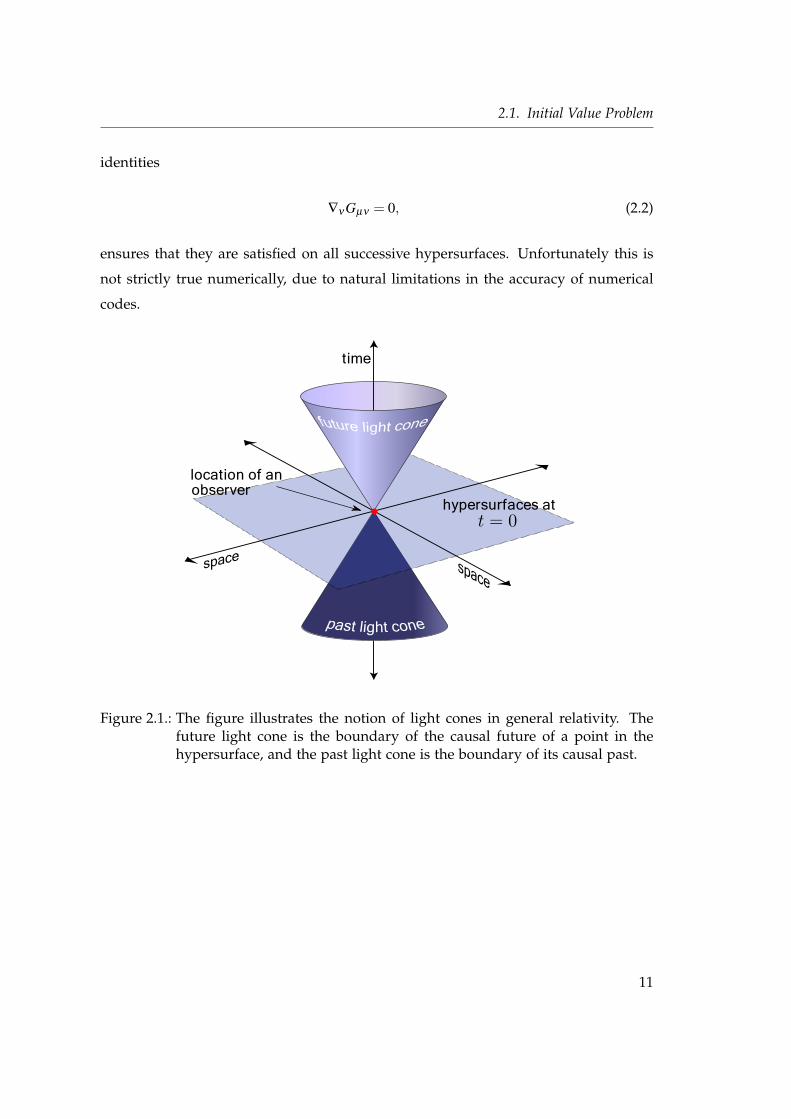
ensures that they are satisfied on all successive hypersurfaces. Unfortunately this is
not strictly true numerically, due to natural limitations in the accuracy of numerical
codes.
time
location of anobserver
hypersurfaces at
Figure 2.1.: The figure illustrates the notion of light cones in general relativity. Thefuture light cone is the boundary of the causal future of a point in thehypersurface, and the past light cone is the boundary of its causal past.
11
2. The 3+1 Split and Initial Data
2.2. The 3+1 Decomposition - Separating Space from Time
As outlined in the previous section the Einstein equations written in their usual form
are manifestly covariant, time and space only appear as equal partners, i.e. as space-
time. This is not only counterintuitive to how humans view the reality but it is also not
a well suited form for numerical simulations, where we need to adopt some quantity
as an evolution parameter. Therefore we will recast Einstein’s equations into a more
convenient form for such a task.
Among the formulations proposed for this purpose, by far the most frequently ap-
plied is the canonical “3+1” decomposition proposed by Arnowitt, Deser and Misner
(ADM) in 1962 [27]. Alternatives such as null, 2+2 or (2+1)+1 (cf. e.g. [28, 29]) splits
have also been studied, but in far less detail than the physically intuitive 3+1 decom-
position. As pointed out in section 2.1 a suitable way to decompose space-time is
the employment of an initial value problem. In the ADM formalism the space-time
is disjoint into a 1-parameter family of 3-dimensional space-like hypersurfaces and
constraints satisfying initial data are provided on one hypersurface in the form of the
spatial 3-metric and its time derivative.
In fact, there have been many modifications to the original ADM formulation, but
the main ideas of ADM still form the basis of standard approaches to numerical rel-
ativity. Our derivation of the evolution equations closely follows the textbook Grav-
itation by Misner, Thorne and Wheeler. An alternative derivation can be found in
Appendix A.
2.3. The ADM Formalism
The field variable in General Relativity is the 4- dimensional space-time metric gµν
defined on a Manifold M . Appropriate initial data can be determined via the well-
known Hilbert variational principle. In general relativity we start from the Einstein-
Hilbert action
SEH =∫
d4x√−gR, (2.3)
12
2.3. The ADM Formalism
where g is the determinant of the 4-dimensional metric and R is the Ricci scalar of
an otherwise empty space. By varying the lagrangian density £ =√−gR in Eq. (2.3)
with respect to the space-time metric gµν we derive the covariant vacuum Einstein
equations with the dynamics encoded in the set of differential equations. We separate
the spatial degrees of freedom from the time-like degrees of freedom and introduce
the ADM quantities,
γi j = gi j, (2.4a)
α = (−g tt)12 , (2.4b)
βi = g0i, (2.4c)
πi j =
√|g|(Γ
0kl− γkl Γ
0mn γ
mn)γ
ikγ
jl. (2.4d)
Arnowitt, Deser and Misner called these quantities the spatial three-metric γi j, the lapse
function α , the shift vector β i and the conjugate momenta π i j, respectively. In the ADM
formalism these quantities acquire a clear physical meaning, as illustrated in Fig. (2.2).
In fact, we may choose a time-like vector tµ to coincide with the normal vector nµ to
the hypersurfaces, but that might not be strictly true, therefore in general
tµ = αnµ +βµ . (2.5)
Here the lapse α encodes the proper distances of the slices as measured by an ob-
server moving perpendicular to the slice, whereas the shift β i lies in the surface Σ and
describes the displacement away from the hypersurface. The three-metric γ i j can be
defined as the projection into Σ. We can invert this system of equations (2.4) and arrive
at the following construction of the 4-metric out of the 3-metric and the lapse and shift
functions
g00 = βkβk−α
2, (2.6a)
g0 j = β j, (2.6b)
gi0 = βi, (2.6c)
gi j = γi j. (2.6d)
13
2. The 3+1 Split and Initial Data
The contravariant space-time metric reads
g00 = −1/α2, (2.7a)
g0 j = βj/α
2, (2.7b)
gi0 = βi/α
2, (2.7c)
gi j = γi j−β
iβ
j/α2. (2.7d)
If we substitute (2.4a) - (2.4d) into (2.3) we derive the Einstein-Hilbert action
SEH =−∫
dx[
γi j∂tπi j +αH +βiPi +2∂i
(π
i jβ j−
12
πβi +∇
iα√
γ
)], (2.8)
where
H = −√
γ
(R+
1γ
(12
π2−π
i jπi j
)), (2.9a)
Pi = −2∇ j πi j, (2.9b)
are the constraint equations, namely the hamiltonian and momentum constraint, re-
spectively. The last term in Eq. (2.8) is a spatial divergence which does not contribute
to the classical equations of motion. The dynamics are encoded in the resulting evo-
lution equations
∂tγi j = 2αg−12
(πi j−
12
γi jπ
)+∇ j βi +∇i β j, (2.10a)
∂tπi j = −α
√γ
(Ri j− 1
2γ
i jR)
+12
αγ− 1
2 γi j(
πmn
πmn−12
π2)
−2αγ− 1
2
(π
inπ
jn −
12
ππi j)
+√
γ(∇
i∇
iα− γ
i j∆α)
+∇n(π
i jβ
n)−πn j
∇nβi−π
ni∇nβ
j, (2.10b)
where ∇ is the covariant derivative associated with γ i j and Ri j is the Ricci tensor
associated with γi j.
York performed a modification to the original ADM equations, introducing the ex-
14
2.3. The ADM Formalism
Figure 2.2.: The foliation of space-time in the ADM 3+1 split showing the lapse func-tion α and shift vector β i for the displacement of a point embedded insuccessive hypersurfaces Σ labeled by a number t with the 3-dimensionalmetric γi j.
trinsic curvature or second fundamental form Ki j:
Ki j =−γ−1/2 (πi j− γi jπ) , (2.11)
where Eq. (2.11) shows the relation between πi j and Ki j.
Rather than evolving the canonically conjugate momenta πi j, York chose the ex-
trinsic curvature Ki j of the three dimensional slices as an evolution variable. In pure
geometrical terms, the extrinsic curvature quantifies roughly the “bend” of a hyper-
surface as measured from a higher dimensional space in which the hypersurface is
embedded. In mathematical terms, we define the extrinsic curvature by applying the
projection tensor on the covariant derivative of the normal vector ∇ν nµ :
Ki j ≡−12
£nγi j, (2.12)
where £n denotes the Lie derivative along the nµ direction. By combining the Gauss-
15
2. The 3+1 Split and Initial Data
Codazzi relations, which define the extrinsic curvature on a sub-manifold, with the
Einstein equations one can derive the vacuum evolution equations for Ki j and γ i j,
respectively (cf. Appendix A):
∂tγi j = −2αKi j +Oiβ j +O jβi (2.13a)
∂tKi j = αRi j−2KilKlj +KKi j−OiO jα +£β Ki j, (2.13b)
where K is the trace of Ki j.
The Hamiltonian and momentum constraints in Eq. (2.9) turn out to be
R+K2−Ki jKi j = 0, (2.14a)
∇ j(Ki j− γ
i jK)
= 0, (2.14b)
giving the well-known form of the constraint equations in numerical relativity.
2.4. BSSN - An Alternative
The ADM evolution equations introduced in the previous section are in fact highly
non-unique. As long as we satisfy the constraints in Eqs. (2.14), there is no restric-
tion at all that prohibits adding arbitrary multiples of the constraints to the equations.
The physical solutions will not change, but the mathematical properties may alter
seriously. As an example, we already demonstrated how the equations may be refor-
mulated, as done by York. It has been shown that the reformulation by York behaved
better mathematically concerning its constraints violating behavior.
But by the late 1990s’, the community finally realized that even York’s formulation was
a rather unsuitable scheme for numerical black hole evolutions, due to its weak hy-
perbolicity [30]. An alternative to ADM was first suggested by Shibata and Nakamura
in 1995 [31] and made popular by a subsequent paper by Baumgarte and Shapiro in
1999 [32]. Baumgarte and Shapiro investigated the stability properties of the Shibata-
Nakamura formulation and showed the remarkable advantage compared with the
standard ADM formulation. The scheme has since become known as the BSSN formal-
16
2.4. BSSN - An Alternative
ism, and is nowadays almost exclusively used in numerical simulations. With these
fundamental ingredients a major breakthrough concerning long-term binary black
hole simulations was achieved in 2001 by two independent groups [33, 34]. Research
in improving schemes continues and today there is no consensus, as to which formu-
lation is the best for numerical purposes. Here we want to give a short overview of
the fundamental equations of BSSN.
The first step to reformulate the ADM equations is the conformal split where we
redefine the determinant of the physical three-metric
φ =112
logg, (2.15)
which enables us to rewrite the space-time metric by introducing the conformal metric
gi j:
gi j = e−4φ gi j, (2.16)
where now det(gi j) = 1. In geometrical terms, the decomposition splits the geometry
into “transverse” and “longitudinal” degrees of freedom (encapsulated by gi j and φ ,
respectively.) We extend this idea to the extrinsic curvature yielding
Ki j = e−4φ Ki j (2.17a)
K = gi jKi j = gi jKi j. (2.17b)
As it is obvious from Eq. (2.17b) scalar quantities like the trace of the extrinsic curva-
ture are not affected by the transformation.
The next step is to separate the trace-free part of the extrinsic curvature in the
following manner
Ai j = e−4φ
(Ki j−
13
gi jK)
, (2.18)
where Ki j represents the “longitudinal” part and the trace-free tensor Ai j the “trans-
verse” part, respectively.
17
2. The 3+1 Split and Initial Data
These two steps are meaningless unless the evolution equations are affected in a
non-trivial manner. A crucial step is to introduce some variables representing spatial
derivatives:
Γi = gab
Γiab. (2.19a)
The evolution equations for these new BSSN fields can then be worked out:
∂t g i j = −2α Ai j +£β g i j, (2.20a)
∂tφ = £β φ − 16
αK, (2.20b)
∂t Ai j = £β Ai j + e−4φ [−∇i∇ j α +α Ri j]TF +α
(K Ai j−2 Aik Ak
j
), (2.20c)
∂t K = £β K−∇i∇ j α +α
(Ai jAi j +
13
K2)
, (2.20d)
∂t Γi = g jk
∂ j∂kβi +
13
γi j
∂ j∂kβk +β
j∂ jΓ
i− Γj∂ jβ
i +23
Γi∂ jβ
j
−2Ai j∂ jα +2α
(Γ
ijkA jk +6Ai j
∂ jφ −23
gi j∂ jK
). (2.20e)
This decomposition has greatly extended evolution times in black hole simulations, in
particular together with the puncture approach [35].
In fact, there are many other possible adjustments that can be made to the BSSN
system that affect its stability properties. For example, the conformal connection has
been modified in various formulation and the original expression in Eq. (2.20e) has
been abandoned. A detailed derivation of possible formulations goes beyond the
scope of this work, for which we like to recommend an article by Yoneda & Shinkai
([30], and subsequent work) about the stability properties of slicing formulations.
18

19

20
3. Gravitational Waves
If the universe is expanding, why can’t I find a parking space?
Woody Allen
General relativity is consistent with special relativity in many respects, and in par-
ticular with the principle that nothing can travel faster than light in vacuum. As a
consequence, space-time perturbation must propagate in a certain fashion. In general
relativity, as demonstrated by Einstein, these perturbation propagate at exactly the
speed of light and are denoted as gravitational waves.
The most natural starting point for any discussion of gravitational waves is the
linearized theory, where one can keep only linear terms in Einstein’s field equations.
3.1. The Linearized Theory of Gravity
This “linearized gravity” is an important theory in its own right and an adequate
approximation to general relativity in the so-called “weak field”, where the space-
time metric gµν only slightly deviates from a flat metric ηµν :
gµν = ηµν +hµν +O(|hµν |2
), |hµν | 1. (3.1)
Here ηµν is defined to be the Minkowski metric (−1,1,1,1) and |hµν | is the magnitude
of a small perturbation to the flat space-time. In fact, it is precisely this “linearized
theory of general relativity” that one obtains in classical field theory for particles of
zero rest mass and spin two in flat space.
21
3. Gravitational Waves
Fortunately, it is rather easy to find an example of a system where we deal with a
small perturbation to an otherwise flat space-time. The conditions above are satisfied
just by looking in our Solar system. Measuring the deviation away from flat space, for
instance on the surface of the Sun, we yield
|hµν | ≈ |h00|.Msun
Rsun≈ 10−6. (3.2)
We might come to the misleading conclusion expecting a gravitational wave with an
enormous amplitude, namely |h| ≈ 10−6. In fact, gravitational waves are only defined
far away from the sources in an otherwise empty space-time. In the case of the earth-
sun system the minimum distance to find waves is roughly R≈ 1ly, and since |hµν | ∝
R−1 typical amplitudes will be |hµν | ≈ 10−26.
By taking a closer look at the approximation we will see that the perturbation hµν
encapsulates not only gravitational waves, but additional, non-radiative degrees of
freedom as well.
As mentioned earlier we shall restrict our attention to linear terms in the perturba-
tion and thus we shall neglect terms of second order or higher in hµν . Moreover, we
will impose a suitable outer boundary condition assuming the space-time is asymp-
totically flat (asymptotically “Minkowskian”)
limr→∞
hµν = 0, (3.3)
where r denotes a radial parameter.
To derive linearized theory from general relativity we start by defining the con-
travariant form of the metric perturbation hµν via
hµν ≡ ηµσ
ηνρhσρ , (3.4)
where it is true that (ηµρ +hµρ
)(η ρν −hρν) = δ
νµ , (3.5)
22
3.1. The Linearized Theory of Gravity
from what we derive the contravariant form of the full metric
gµν = ηµν −hµν . (3.6)
The connection coefficients (Christoffel symbols), when linearized in hµν , read
Γµ
αβ= gµσ
Γσαβ =12
gµσ(gσα ,β + gβσ ,α − gµα ,σ
)=
12
(η µσ − hµσ )((ησα + hσα) ,β + (ηβσ + hβσ ) ,α − (ηµα + hµα) ,σ
)' 1
2η
µσ(hσα ,β + hβσ ,α − hµα ,σ
)+O
([hµν
]2). (3.7)
The operation of raising and lowering the indices is performed by using ηµρ and
η µρ , not the full metric, which is a consequence of linearization. Once the Christoffel
symbols are computed we can calculate the Ricci tensor and Ricci scalar to linear order,
yielding
Rµν = Γσµν ,σ − Γ
σµσ ,ν
=12(h σ
µ ,νσ + h σν ,µσ − h σ
µν ,σ − hµν
), (3.8)
and
R =(hµσ
,µσ − h σσ
). (3.9)
Finally, the linearized Einstein tensor turns out to be
Gµν = Rµν −12
ηµν R (3.10)
=12(h σ
µσ ,ν + h σνσ ,µ − h σ
µν ,σ − hµν − ηµν
(h σρ
σρ, − h σ, σ
))= 0
Note that the same result can be achieved by utilizing the variational principle as in
chapter 2.
The expression in Eq. (3.10) is a bit unwieldy and does not seem yet to suggest any
sort of wave-like behavior we would normally expected for a “wave”. Somewhat re-
23
3. Gravitational Waves
markably, this behavior can be significantly unveiled by changing the notation: rather
than working with the metric perturbation hµν , we use the trace-free metric perturba-
tion defined as
hµν = hµν −12
ηµνh. (3.11)
We can perform such a transformation without loss of generality since Eq. (3.11)
merely presents a gauge transformation. With this new notation the field equations
Gµν = 8π Tµν take the form
− h αµν ,α − ηµν h αβ
αβ , + h αµα, ν + h α
να, µ = 16π Tµν . (3.12)
The first term on the left hand side of Eq. (3.12) is the usual d’Alembertian (or wave)
operator
hµν = h αµν ,α , (3.13)
whereas the other terms are merely pure gauge. Due to this fact we exploit the gauge
freedom inherent to general relativity to recast (3.13) in a more accessible form. With-
out loss of generality we can impose a gauge condition in such a way to eliminate the
terms that spoil the wave-like nature, in particular by choosing
hµα
,α = 0. (3.14)
Making use of the gauge, which is mostly wrongly called the Lorentz gauge1 , the
linearized field equations then become
hµν = h αµν ,α = 0, (3.15)
clearly showing the wave-like nature of the gravitational field if matter is absent (i.e.
if Tµν = 0).
1The Lorenz gauge condition is named after Ludvig Lorenz and is frequently misspelled because ofconfusion with Hendrik Lorentz, after whom Lorentz invariance is named.
24
3.1. The Linearized Theory of Gravity
Figure 3.1.: This is an image of the sky as viewed by gravitational waves. The MilkyWay galaxy forms the band in the middle of the image. LISA will seethousands of binary star systems in our galaxy, and will be able to deter-mine the direction and distance to each binary, as well as the periods ofthe orbits and the masses of the stars. (Beyond Einstein Roadmap)
25
3. Gravitational Waves
3.2. A Wave Solution and the Transverse-Traceless Gauge
The field equations of linearized theory bear a close analogy to the equations of elec-
trodynamics, consequently we can infer much about linearized theory. Tracking this
analogy, it is not surprising that the simplest solution to the linearized wave equation
(3.15) is that of a monochromatic plane wave:
hµν = ℜ
[Aµν e iκσ xσ
], (3.16)
where ℜ [...] denotes the real part, Aµν is the amplitude tensor and the wave-vector κ
is light-like, κµκµ = 0. The Lorenz gauge condition implies that the amplitude and
the wave-vector are orthogonal Aµν κν = 0. Evidently, in such a solution, the plane
wave in Eq. (3.16) travels in the spatial direction ~k = (κx,κy,κz)/κ0 with frequency
ω = κ0 =√
(κ iκi).
As mentioned before, linearized gravity can be described within classical field the-
ory by a massless spin-2 field that propagates with the speed of light. We know from
field theory that such a field has only two independent degrees of freedom (“helici-
ties” in quantum theory, and “polarizations” in a classical description). On the other
hand, one might come to the conclusion that the symmetric tensor Aµν of this plane
wave appears to have 16−6 = 10 free components. But as we will demonstrate, there
are in fact really just two dynamical degrees of freedom in linearized relativity. The
“excess” is due to the arbitrariness tied up in the gauge freedom; by choosing a par-
ticular gauge, namely the TT gauge, one gets rid of the remaining unwanted degrees
of freedom and one is only left with the two dynamical degrees. One can impose the
following conditions:
(I) Lorenz gauge conditions: Since we impose the Lorenz gauge condition
Aµν κν = 0, (3.17)
4 components of the amplitude tensor can be specified.
(II) Global Lorentz Frame: Just like in special relativity one can select a four-velocity
26
3.2. A Wave Solution and the Transverse-Traceless Gauge
u - the same through all space-time and define a global Lorentz frame where one can
impose the conditions:
Aµν uν = 0. (3.18)
These are only three constraints on Aµν not four, because one of them,
κµ Aµν uν = 0, (3.19)
is already fulfilled by the Lorenz gauge condition.
(III) Diffeomorphism Condition: We can impose an infinitesimal gauge transforma-
tion in such a way to set
A µ
µ = 0. (3.20)
We can translate these conditions in Eqs. (3.17 , 3.18 , 3.20) to constraints for the
perturbation tensor hi j by considering a reference Lorentz frame where u0 = 1, ui = 0
(globally at rest), and where κ µ does not appear directly:
(I) h i j, j = 0, i.e., the spatial components are divergence free,
(II) hµ0 = 0, i.e., only the spatial components hi j are non-zero,
(III) h ii = 0, i.e., the spatial components are trace-free.
Together these conditions define the so-called Transverse Traceless gauge (TT).
Even if there is no need in general relativity to prefer one gauge over another, it is ex-
tremely convenient to choose the TT-gauge, since it fixes all the local gauge freedom,
therefore eliminating unphysical degrees of freedom. Thus, the metric perturbation
hT Tµν contains only physical, non-gauge information about the radiation.
To be able to interpret the effects of the metric perturbation hT Tµν , we calculate the
Riemann tensor in the transverse-traceless gauge, which encodes the curvature of the
underlying space-time. It turns out that the only non-zero components of the Riemann
tensor are
R j0k0 = R0 j0k =−R j00k =−R0 jk0, (3.21)
27

3. Gravitational Waves
and the explicit expressions of the components of the linearized Riemann tensor read
R j0k0 =−12
hT Tjk,00. (3.22)
These important relations between the metric perturbation and the components of
the Riemann tensor in linearized general relativity facilitate to associate a traveling
gravitational wave with a local oscillation of the space-time!
3.2.1. Interaction of Gravitational Waves with Test-Particles
With the results from the foregoing sections we are now able to calculate the effect
of a gravitational wave on a freely falling particle following a geodesic in space-time.
First, we will demonstrate how an unsuitable coordinate choice can lead to incorrect
results, and therefore indicate how important it is to rely on coordinate independent
quantities such as the Weyl scalars.
The motion of a particle is given by the usual geodesic equation without external
forces
d2xµ
dτ2 +Γµ
ρσ
dxρ
dτ
dxσ
dτ= 0, (3.23)
where τ is the proper time of the particle. We can rewrite the equation combining the
time-like with the spatial part of the 4-vector xµ yielding an equation for the coordinate
acceleration:
d2xi
dt2 =−(
Γitt +2Γ
it jv
j +Γijkv jvk
)+ vi
(Γ
ttt +2Γ
tt jv
jΓ
tjkv jvk
). (3.24)
Let us now restrict our attention to linearized theory written in TT-gauge and further
assume the velocity of the test particle is rather slow (v 1). As a valid approximation
we can neglect the velocity dependent terms in Eq. (3.24), yielding the simplified
equation:
d2xi
dt2 =−Γitt , (3.25)
28
3.2. A Wave Solution and the Transverse-Traceless Gauge
where we now compute the Christoffel symbol Γ itt in the TT-gauge to lowest order
yielding the surprising result
d2xi
dt2 =−Γitt =
12(2∂thT T
jt −∂ jhT Ttt)
= 0, (3.26)
since hT Tµt = 0 (global Lorentz frame condition). A naive interpretation of the result
would be that the test particle is not influenced by a passing gravitational wave! This
is certainly wrong, but is a clear example how important a careful coordinate choice in
general relativity can be. Even more importantly is to focus upon coordinate invariant
quantities like the Weyl scalars. We will introduce these scalar quantities in chapter 4.
To return to our example, we will now show that in fact traveling gravitational waves
produce oscillations in the separation between neighboring objects. As a gravitational
wave passes, it perturbs the geodesic motion of the two particles and contributes to
the geodesic deviation equation. To examine the action of the wave on the separation
of freely falling test particles we start by introducing a locally flat coordinate system
xa, attached to the world line of a particle A. The line element takes the form
ds2 =−dτ2 +δ i j dxi dx j +O(|x j|2) dx α dx β , (3.27)
where the first and second term on the right-hand side correspond to Minkowski-flat
space and the the last term on the right-hand site encodes the deviation from the
geodesic motion.
We start by introducing the geodesic-deviation equation
uγuβ nα
;βγ=−Rα
βγδuβ uδ nγ , (3.28)
where n is the separation four-vector between two geodesic trajectories with tangent
vector u. Additionally, we define the separation vector as n j ≡ x jB− x j
A, reaching from
particle A to particle B. With this definition the geodesic-deviation equation can be
expressed asd2n j
dτ2 =−R j0k0
nk, (3.29)
29
3. Gravitational Waves
and with setting x jA = 0 the geodesic-deviation equation simplifies to
d2x jB
dτ2 =−R j0k0
x kB. (3.30)
Since we want to carry out the results in the TT-gauge we use the definition of the
Riemann tensor in Eq. (3.22) yielding
d2x jB
dτ2 =12
∂ 2hT Tjk
∂ t2 x kB, (3.31)
with the solution
x jB(t) = x k
B(0)[
δi j +12
hT Tjk (t)
]. (3.32)
In contrast to the solution in Eq. (3.26) the result above has a straightforward and
meaningful interpretation; particle B is seen oscillating with an amplitude propor-
tional to the time-dependent metric perturbation hT Tjk
(t).
3.2.2. Polarization of a Plane Wave
As discussed in the foregoing sections gravitational waves are transverse in linearized
theory and the two remaining degrees of freedom can be associated with two different
polarizations. To construct the possible polarizations of gravitational wave we start by
considering a plane wave propagating with the speed of light along the positive x-axis.
Thus, for the particular example the perturbation metric tensor in TT-gauge is defined
as
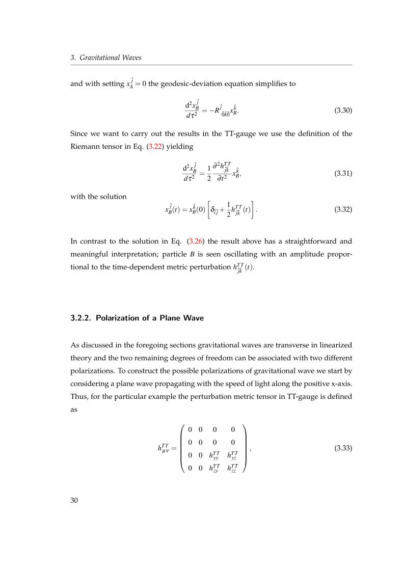
hT Tµν =
0 0 0 0
0 0 0 0
0 0 hT Tyy hT T
yz
0 0 hT Tzy hT T
zz
, (3.33)
30
3.2. A Wave Solution and the Transverse-Traceless Gauge
AB
Figure 3.2.: The figure illustrates how the arrival of a gravitational wave propagatingalong the direction~k perturbs the geodesic motion of two particles A andB.
with the only non-vanishing components
hT Tyy = −hT T
zz = ℜ
[A+ e−iω(t−x)
](3.34a)
hT Tyz = hT T
zy = ℜ
[A× e−iω(t−x)
](3.34b)
where A+ and A× represent the amplitudes of two independent modes of polarization.
As we already know from classical electrodynamics, we can recast such a planar wave
into two linearly polarized plane waves or, by superposing the linear polarizations,
into two circularly polarized ones. We call these linear polarizations “+” (“plus”) and
“×” (“cross”) -polarizations. The unit linear-polarization tensors are called e+ and e×,
respectively, and may be written as
e+ ≡ ~ez⊗~ez−~ey⊗~ey, (3.35a)
e× ≡ ~ez⊗~ey +~ey⊗~ez. (3.35b)
31
3. Gravitational Waves
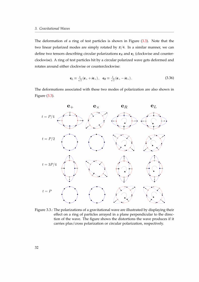
The deformation of a ring of test particles is shown in Figure (3.3). Note that the
two linear polarized modes are simply rotated by π/4. In a similar manner, we can
define two tensors describing circular polarizations eR and eL (clockwise and counter-
clockwise). A ring of test particles hit by a circular polarized wave gets deformed and
rotates around either clockwise or counterclockwise:
eL ≡ 1√2(e+ + ie×) , eR ≡ 1√
2(e+− ie×) . (3.36)
The deformations associated with these two modes of polarization are also shown in
Figure (3.3).
Figure 3.3.: The polarizations of a gravitational wave are illustrated by displaying theireffect on a ring of particles arrayed in a plane perpendicular to the direc-tion of the wave. The figure shows the distortions the wave produces if itcarries plus/cross polarization or circular polarization, respectively.
32
3.3. Interaction of Gravitational Waves with Detectors
3.3. Interaction of Gravitational Waves with Detectors
To detect a gravitational wave there are two basic and very different methods available.
One is by measuring the energy deposited by the wave in a resonant-mass detector
and is based on the pioneering work by Joseph Weber [36]. The other principle is by
measuring the change in time it takes light to travel between two distinct locations.
Here we want to concentrate on the beam detectors2.
The measurement technique of beam detectors is based on an interferometric mea-
surement with a Michelson interferometer operated with highly stabilized laser light.
To have a reasonable detection rate of astronomical sources these detectors must be
able to measure changes in its arm-length that are smaller than 1 part in 10−21 (cf. e.g.
[37]). Currently four earth-based laser-interferometric detectors are taking real data.
These are TAMA [38], GEO600 [39], LIGO [40], and VIRGO [41].
TAMA is a Japanese detector, with an arm-length of 300m, assembled near Tama,
Tokyo. It was the first large scale laser-interferometric gravitational wave detector to
have taken scientific data in September 1999. The current sensitivity is 10−21/√
Hz at 1
kHz. With such a sensitivity it is possible to detect gravitational waves from coalescing
neutron-star binaries in our galaxy.
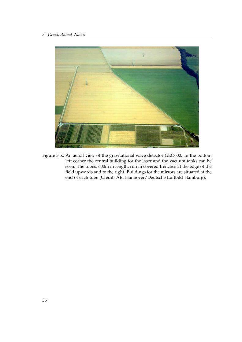
GEO600 is a British-German detector with 600m long arms constructed in Germany
close to Hannover. The light is folded once in both arms increasing the light path to
1200m in each arm. The current sensitivity is 2×10⁻²²/√
Hz between 400 and 500 Hz.
LIGO is situated in the USA and consists of three long-baseline interferometers on
two sites, one (4km/2km arm-length) at the Hanford Reservation near Washington
and the other (4km arm-length) is situated at Baton Rouge, Louisiana. The current
sensitivity is 2×10⁻²³/√
Hz between approximately 100 and 200 Hz. LIGO now moves
into its next phase of progress, Enhanced LIGO. This consists of a set of upgrades and
hardware improvements designed to extend the astrophysical reach.
VIRGO is a French-Italian detector with 3 km long arms situated close to Pisa in
Italy. The design sensitivity is 3×10⁻²¹/√
Hz at 1 Hz and 3×10⁻²³/√
Hz at 1 kHz.
2For an exhaustive overview over different detectors and related technical issues we would like to referto a textbook by Ciufolini et al. [37]
33
3. Gravitational Waves
Below about 1 Hz gravity gradient noises (i.e. tidal forces) are stronger than any
gravitational wave from astrophysical objects we can expect in this frequency regime
to detect on earth. This is one main reason why scientists proposed the LISA mission
in the early nineties [42].
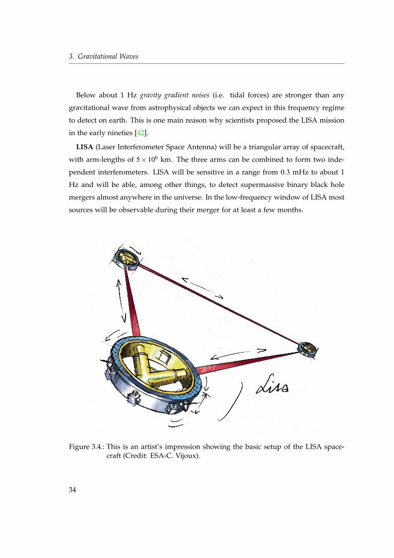
LISA (Laser Interferometer Space Antenna) will be a triangular array of spacecraft,
with arm-lengths of 5× 10⁶ km. The three arms can be combined to form two inde-
pendent interferometers. LISA will be sensitive in a range from 0.3 mHz to about 1
Hz and will be able, among other things, to detect supermassive binary black hole
mergers almost anywhere in the universe. In the low-frequency window of LISA most
sources will be observable during their merger for at least a few months.
Figure 3.4.: This is an artist’s impression showing the basic setup of the LISA space-craft (Credit: ESA-C. Vijoux).
34
3.3. Interaction of Gravitational Waves with Detectors
These facilities are not competing with each other but in contrast are forming a
network of detectors. Apart from the fact that only a simultaneous detection in at
least two detectors can be trusted, only a network of detectors is able to conduct full
information of a gravitational wave. The information consists of five quantities; the
amplitude of the wave, the phase between the two polarizations, and the position
of the source, expressible in two angles. To derive these parameters at least three
detectors need to measure a gravitational wave simultaneously.
To describe the way in which a interferometric detector works, suppose one arm
of a beam detector, like GEO600, lies along the z-axis and the wave, for simplicity, is
propagating down the x-axis with a “plus” polarization. Assume further that the two
neighboring particles are located at x = x0 = 0, and are separated on the z-axis by a
distance LD. The proper distance L between the two neighbored particles is then given
by
L =∫ LD
0dx√
gzz =∫ LD
0dx√
1+hT Tzz (t,x0)≈ LD
[1+
12
hT Tzz (t,x0)
]. (3.37)
The fractional length change δL/L can be measured via interferometric instruments
and is given by
δLL≈ 1
2hT T
zz (t,x0) . (3.38)
Even if this is a simple example it clearly shows the fundamental way a interferometric
detector works. An obvious advantage of beam detectors is that the effect induced by a
gravitational wave can be made larger simply by increasing the arm length as directly
seen from Eq. (3.38). For example, assume a detector like LIGO with an arm-length L
of approximately L = 4 km measures a gravitational wave with a strain amplitude of
10−21 and the directional dependences as described above. The measured fractional
change will be as small as
δL≈ 2×10⁻¹⁸m, (3.39)
which is less than 1/1000 the diameter of a proton and, unfortunately, corresponds to
the largest effects we can expect from astrophysical sources.
35
3. Gravitational Waves
Figure 3.5.: An aerial view of the gravitational wave detector GEO600. In the bottomleft corner the central building for the laser and the vacuum tanks can beseen. The tubes, 600m in length, run in covered trenches at the edge of thefield upwards and to the right. Buildings for the mirrors are situated at theend of each tube (Credit: AEI Hannover/Deutsche Luftbild Hamburg).
36
3.4. The Energy of Gravitational Radiation
3.4. The Energy of Gravitational Radiation
We now understand how gravitational waves emerge from the theory of general rel-
ativity and what kind of polarization a wave may have. But besides measuring the
amplitude and phase of the polarizations, we can estimate the energy flux associated
with a gravitational wave which, in general, may be extracted by a detector. Un-
fortunately, the energy is rather ill-defined in linearized theory and additionally the
stress-energy cannot be localized inside a certain region of the wave package. To de-
rive an expression for the energy flux it is necessary to assume being far from the
emitting object, i.e. to reside in an otherwise flat space-time. We start by examining
the form of the stress-energy tensor in the TT-gauge, the Issacson tensor
Tµν =1
32π
⟨∂µhT T
i j ∂νhT Ti j⟩, (3.40)
where 〈...〉 denotes an average over the metric perturbations. The usual definition of
the energy flux by solid angle is
∂ 2E∂ t∂Ω
= limr→∞
r2T rt . (3.41)
Combining Eq. (3.40) and Eq. (3.41) we yield a possible estimation of the energy flux
of a gravitational wave in the TT-gauge
∂ 2E∂ t∂Ω
= limr→∞
r2
16π
(∂hT Tθ θ
∂ t
)2
+
(∂hT T
θ φ
∂ t
)2 . (3.42)
37
3. Gravitational Waves
3.5. Gravitational Waves from Perturbed Black Holes
One of the most interesting astrophysical sources of gravitational waves are black holes
in the centers of galaxies. These are supermassive objects with up to 108 solar masses
[43, 44, 45]. Such supermassive black holes are now believed to be common in centers
of active galactic nuclei (AGN), and there is compelling evidence for at least one black
hole of around three million solar masses in the center our own galaxy [46, 47, 48, 49].
Perhaps the most absorbing source involving massive black holes is their merger
during a galactic merger process. Such an event from anywhere in the universe “must”
be visible to LISA with very high signal-to-noise ratios. This will be a fundamentally
important objective because if unseen by LISA, it would cause us to re-evaluate the
very existence of gravitational waves.
The only remnant of such a merger allowed by general relativity is a more massive
black hole with a perturbed event horizon. Gravitational waves from perturbed black
holes are distinctive and reduce to a simple wave equation, which has been studied
extensively [9, 10, 50, 51, 52, 53, 54]. They will carry a unique fingerprint which would
lead to the direct identification of their existence.
3.5.1. Perturbation Theory and Quasi-Normal Modes
We will briefly review fundamental perturbations that characterize black holes with-
out explicit derivation3. We have to restrict ourself to non-rotating black holes due
to the fact that for the Kerr solution the analysis is highly complicated (beside being
partly still unknown). Some of the main results date back in the 70’s with first stud-
ies by Regge, Wheeler and Zerilli [9, 10]. In fact, a variety of perturbation schemes
have been developed, but we want to focus our attention on the most important ap-
proaches. We will introduce a novel approach in chapter 4 which is based on the
Newman-Penrose null-tetrad formalism, in which the tetrad components of the cur-
vature tensor are the fundamental variables.
The results obtained in the middle of the nineteenth century raised considerable
surprise and doubts at first. The idea that black holes oscillate and possess some
3For a good review we recommend an article by K. Kokkotas and B. Schmidt [55]
38
3.5. Gravitational Waves from Perturbed Black Holes
Figure 3.6.: One of the most violent astrophysical events: the merging of two blackholes. (Image: MPI for Gravitational Physics/W.Benger-ZIB)
proper modes of vibration seemed rather awkward since it is not a material object, it
is a singularity hidden by a horizon.
The procedure is very similar to the analysis carried out in linearized theory (cf.
section 3.1); we deal with a static vacuum Schwarzschild space-time g0µν superposed
with a small perturbation hµν which encodes the deviation from spherical symmetry.
T. Regge and J. A. Wheeler showed that the equations describing the perturbations
of a Schwarzschild black hole can be separated as (cf. section 2.2)
gµν = g0µν +hµν , (3.43)
provided that the perturbed metric tensor can be expanded in tensorial spherical har-
monics. This was possible since in the Schwarzschild case the perturbations naturally
decouple due to spherical symmetry of the space-time. Regge and Wheeler called
the result odd-parity and even-parity solution, respectively. The name odd-parity and
39
3. Gravitational Waves
even-parity emerges from the properties of the tensor spherical harmonics defined as
hµν (t,r,θ ,φ) = ∑l,m
alm(t,r)Almµν(θ ,φ)+blm(t,r)Blm
µν(θ ,φ), (3.44)
with distinctive transformation properties of the functions Almµν and Blm
µν under parity
operations. Later, it was found that the odd perturbations represent really the angular
perturbations to the metric, while the even ones are the radial perturbations to the
metric [53, 56].
The perturbation equations are still commonly used in numerical relativity to extract
the radiation quantities. That is partly due to a lack of serious investigations concern-
ing the error of the method. We conclude this section by quoting Chandrasekhar from
his book The Mathematical Theory of Black Holes and move to the next section where we
will work out the details of the perturbations, also called quasi-normal modes:
..we may expect on general grounds that any initial perturbation will, during its last stages,
decay in a manner characteristic of the black hole and independently of the original cause. In
other words, we may expect that during the very last stages, the black hole will emit gravita-
tional waves with frequencies and rates of damping, characteristic of itself, in the manner of
a bell sounding its last dying pure note. These considerations underlie the formulation of the
concept of the quasi-normal modes of a black hole.
3.5.2. The Regge-Wheeler and Zerilli Equation
The equation for the odd-parity perturbations are known as the Regge-Wheeler equa-
tion, describing the axial perturbations of the Schwarzschild metric in linear approxi-
mation, that is, we can decompose the perturbation hµν in Eq. (3.43) into tensor spher-
ical harmonics according to Eq. (3.44) considering only odd terms. As in section (2.2)
we can calculate the perturbed Einstein tensor, where we assume a time dependence
for the Regge-Wheeler function R(r,ω) and Zerilli function Z (r,ω) of the form
R(r,ω) ∝ eiωnt , Z (r,ω) ∝ eiωnt , (3.45)
40
3.5. Gravitational Waves from Perturbed Black Holes
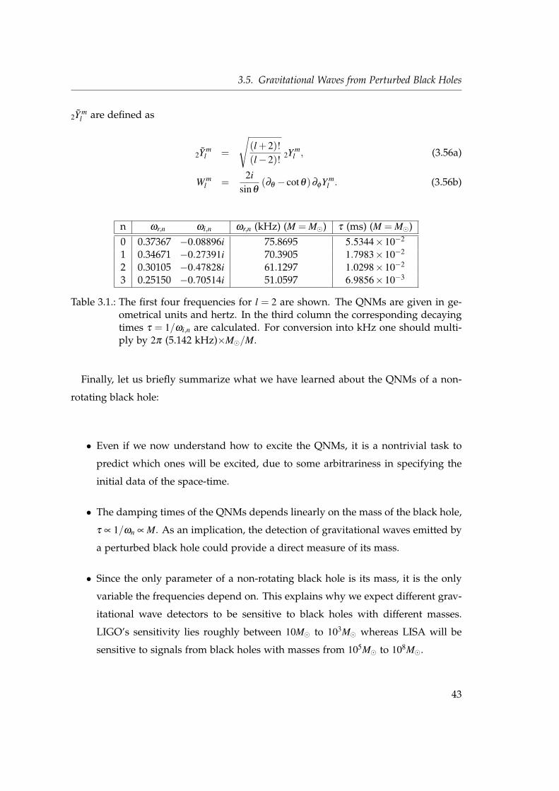
where ωn is the oscillation frequency of the nth mode and is a complex number of the
type
ωn = ωr,n + iωi,n, with n = 0,1,2, ... (3.46)
The explicit derivation goes beyond the scope of this work and leads to no additional
insight. Therefore we solely present and discuss the main results of black hole vibra-
tion modes.
Regge and Wheeler demonstrated that one ends up with three unknown variables,
commonly called h0, h1 and h2. We can set one of the three unknown variables to zero,
namely h2 = 0, by applying a particular gauge transformation, the Regge-Wheeler gauge
[9]. Finally, we are left with the nontrivial Einstein equations to be determined:
ω2n R(r,ωn)+∂
2r∗R(r,ωn)−Vs(r)R(r,ωn) = 0, (3.47)
∂th0−∂r∗ [r∗R(r,ωn)] = 0 (3.48)
where R(r,ωn) is the master variable
R(r,ωn) =h1
r
(1− 2M
r
), (3.49)
and r∗ is the tortoise coordinate r∗ = r + 2M ln( r
2M −1). In general, the time derivative
of R(r,ωn) must also be calculated to provide full Cauchy data for an evolution. The
function Vs(r) is the so-called Regge-Wheeler potential defined as
Vs(r) =(
1− 2Mr
)[l (l +1)
r2 +2M(1− s2
)r3
], (3.50)
where s is the spin of the particle and l is the angular momentum of the specific wave
mode under consideration, with l ≥ s. The spin can take the values s = 0,±1±2 where
the most important cases from astrophysical point of view are s = ±1 and s = ±2,
which describe electromagnetic and gravitational waves, respectively. We can con-
sider the function V (r) as an effective, scattering potential barrier with a peak around
41
3. Gravitational Waves
r = 3.3M, which is the location of the unstable photon orbit.
Next, we look at the even parity case where we yield a similar result for the Einstein
equations commonly called the Zerilli equation
ω2n Z (r,ωn)+∂
2r∗Z (r,ωn)−V Z (r,ωn) = 0, (3.51)
where Z (r,ωn) is the Zerilli master variable and V2(r) is the Zerilli potential
V2(r) =(
1− 2Mr
)[2n(n+1)r3 +6n2Mr2 +18nM2r +18M3
r3 (nr +3M)2
], (3.52)
assuming s = 2 and n = 12(l−1)(l +2).
We may now calculate the response of a black hole to external perturbations as the
solutions of Eq. (3.47, 3.53),
ω2n R(r,ωn)+∂
2r∗R(r,ωn)−Vs(r)R(r,ωn) = 0, (3.53)
ω2n Z (r,ωn)+∂
2r∗Z (r,ωn)−V2(r)Z (r,ωn) = 0. (3.54)
The approach to find the solution for the master variables R(r,ωn) and Z (r,ωn) is based
on the standard WKB treatment of wave scattering at a potential barrier (cf. [57]).
Finally, having found the QNMs of a black hole via the Regge-Wheeler and Zer-
illi approach we can calculate the gravitational wave signal in terms of the master
variables by the formula
hTT+ (t,r,θ ,φ) =
12πr
∫eiωn(t−r∗) ∑
lm
[Z(r,ωn)
(2Y m
l −W ml)+
1ωn
R(r,ωn)W ml
]dωn, (3.55a)
hTT× (t,r,θ ,φ) = − i
2πr
∫eiωn(t−r∗) ∑
lm
[Z(r,ωn)W m
l −1
ωnR(r,ωn)
(2Y m
l −W ml)]
dωn, (3.55b)
where Y ml
(sY m
l
)is the (spin-weighted) spherical harmonics and the functions W m
l and
42
3.5. Gravitational Waves from Perturbed Black Holes
2Y ml are defined as
2Y ml =
√(l +2)!(l−2)! 2Y m
l , (3.56a)
W ml =
2isinθ
(∂θ − cotθ)∂φY ml . (3.56b)
n ωr,n ωi,n ωr,n (kHz) (M = M) τ (ms) (M = M)0 0.37367 −0.08896i 75.8695 5.5344×10⁻²
1 0.34671 −0.27391i 70.3905 1.7983×10⁻²
2 0.30105 −0.47828i 61.1297 1.0298×10⁻²
3 0.25150 −0.70514i 51.0597 6.9856×10⁻³
Table 3.1.: The first four frequencies for l = 2 are shown. The QNMs are given in ge-ometrical units and hertz. In the third column the corresponding decayingtimes τ = 1/ωi,n are calculated. For conversion into kHz one should multi-ply by 2π (5.142 kHz)×M/M.
Finally, let us briefly summarize what we have learned about the QNMs of a non-
rotating black hole:
• Even if we now understand how to excite the QNMs, it is a nontrivial task to
predict which ones will be excited, due to some arbitrariness in specifying the
initial data of the space-time.
• The damping times of the QNMs depends linearly on the mass of the black hole,
τ ∝ 1/ωn ∝ M. As an implication, the detection of gravitational waves emitted by
a perturbed black hole could provide a direct measure of its mass.
• Since the only parameter of a non-rotating black hole is its mass, it is the only
variable the frequencies depend on. This explains why we expect different grav-
itational wave detectors to be sensitive to black holes with different masses.
LIGO’s sensitivity lies roughly between 10M to 103M whereas LISA will be
sensitive to signals from black holes with masses from 105M to 108M.
43
3. Gravitational Waves
• The QNM frequencies of galactic size black holes, like the one at the center of
our own galaxy with masses of 106M, will be in the mHz regime and therefore
detectable only from LISA. Figure (3.7) gives an overview over various sources
detectable by LIGO and LISA, respectively.
Figure 3.7.: The figure shows the strain sensitivity of LIGO and LISA, respectively.Regions where various sources are predicted to be are also shown. (Image:Beyond Einstein Roadmap)
44

45

46
4. The Newman-Penrose Formalism
If I have seen further it is by standing on the shoulders of giants.
Isaac Newton, February 5, 1675
In spite of the advantages of perturbation schemes like Regge-Wheeler [9] or Zerilli
[10] there is a crucial drawback of linear perturbation theory: there is no information
within linearized theory to determine its range of applicability, i.e. to determine which
values are sufficiently small to be treated as a perturbation. These disadvantages may
be resolved by extending the perturbation schemes to a still higher order. Unfor-
tunately, the equations become extremely complicated and that makes it practically
impossible to solve the problem analytically [58].
But even worse, all these perturbation approaches are fundamentally assuming
knowledge of a background metric, in fact, they are well defined only for Schwarzschild
background, formulated in a particular coordinate system. As a natural limitation of
numerical simulations, such a specific knowledge is just not known a-priori. As a re-
sult there is a strong demand for a formalism that does not imply any knowledge of
specific background structures in the first instance.
The Newman-Penrose formalism [11] is a fundamental contribution towards this de-
mand. It has been shown that the introduced curvature quantities in this formalism,
namely the Weyl scalars and the spin coefficients, acquire a direct physical relevance,
carrying all information of the space-time under examination without the need of per-
forming a linearization a priori [16, 59]. Despite its undeniable validity, the equations
governing the formalism are rather complicated and their nature and the connection
between all the equations is yet to be fully understood.
47
4. The Newman-Penrose Formalism
In this chapter we give a general introduction to the underlying mathematical tech-
niques of the Newman-Penrose formalism, the fundamental variables and why it is
regarded as a particular suitable approach to extract the gravitational wave signal in
numerical simulations. In particular, we demonstrate how the transverse Weyl scalars
Ψ4 and Ψ0 can be identified with the outgoing and ingoing gravitational radiation,
respectively.
Afterwards, we discuss recent improvements in theoretical understanding of the
Newman-Penrose formalism [1, 60, 19, 22]. We introduce the notion of the quasi-
Kinnersley frame which assures that we recover the dynamics obeying Teukolsky’s
master equation in the limit of Petrov type D space-time [15]. This will be the ba-
sis to the next two chapters, where we propose a new formalism for wave extraction
and apply our new method to a typical situation in numerical relativity.
4.1. Mathematical Preliminaries
The concept of the tetrad formalism is to introduce a suitable tetrad basis of four
linearly independent vector-fields and project all relevant quantities of the problem
under study on to the chosen basis. The choice of the tetrad basis depends on the
underlying space-time symmetries we wish to exploit. To begin our discussion we
introduce at each point of the Manifold a basis of four vector fields eµ
(i), where i runs
from 1 to 4 designating tetrad indices, and Greek indices denote tensor indices. We
define the covariant form according to
e(i)ν = gµνeµ
(i), (4.1)
where gµν is the metric tensor of the space-time under consideration. In addition, we
can define the inverse of eµ
(i) by
eµ
( j)e(i)µ = δ
(i)( j) and e(i)
µ eν
(i) = δν
µ . (4.2)
48
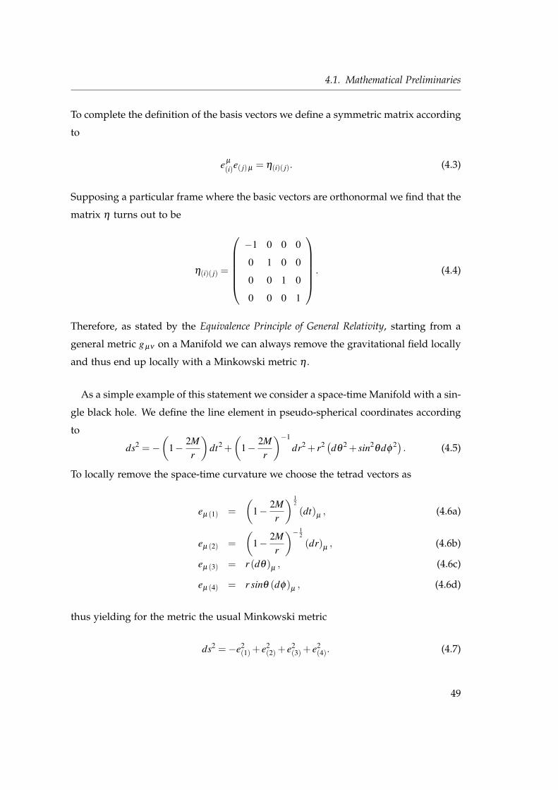
4.1. Mathematical Preliminaries
To complete the definition of the basis vectors we define a symmetric matrix according
to
eµ
(i)e( j)µ = η(i)( j). (4.3)
Supposing a particular frame where the basic vectors are orthonormal we find that the
matrix η turns out to be
η(i)( j) =
−1 0 0 0
0 1 0 0
0 0 1 0
0 0 0 1
. (4.4)
Therefore, as stated by the Equivalence Principle of General Relativity, starting from a
general metric gµν on a Manifold we can always remove the gravitational field locally
and thus end up locally with a Minkowski metric η .
As a simple example of this statement we consider a space-time Manifold with a sin-
gle black hole. We define the line element in pseudo-spherical coordinates according
to
ds2 =−(
1− 2Mr
)dt2 +
(1− 2M
r
)−1
dr2 + r2 (dθ2 + sin2
θdφ2) . (4.5)
To locally remove the space-time curvature we choose the tetrad vectors as
eµ (1) =(
1− 2Mr
) 12
(dt)µ, (4.6a)
eµ (2) =(
1− 2Mr
)− 12
(dr)µ, (4.6b)
eµ (3) = r (dθ)µ, (4.6c)
eµ (4) = r sinθ (dφ)µ, (4.6d)
thus yielding for the metric the usual Minkowski metric
ds2 =−e2(1) + e2
(2) + e2(3) + e2
(4). (4.7)
49
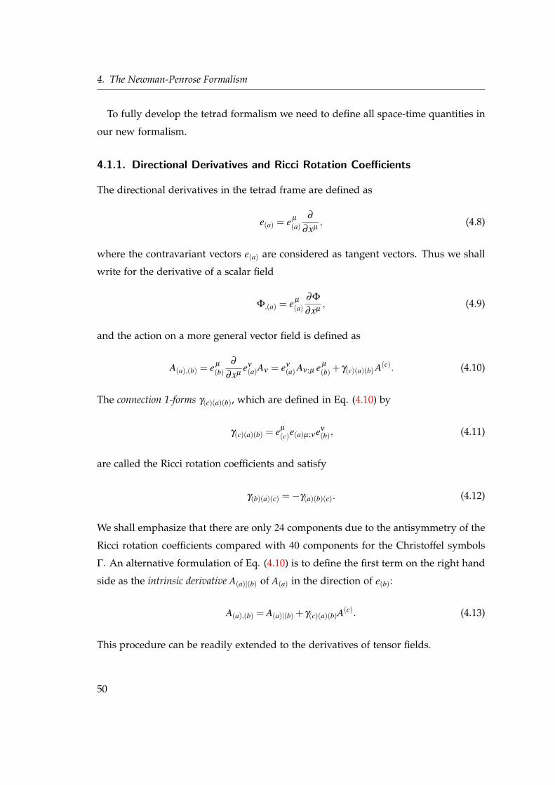
4. The Newman-Penrose Formalism
To fully develop the tetrad formalism we need to define all space-time quantities in
our new formalism.
4.1.1. Directional Derivatives and Ricci Rotation Coefficients
The directional derivatives in the tetrad frame are defined as
e(a) = eµ
(a)∂
∂xµ, (4.8)
where the contravariant vectors e(a) are considered as tangent vectors. Thus we shall
write for the derivative of a scalar field
Φ,(a) = eµ
(a)∂Φ
∂xµ, (4.9)
and the action on a more general vector field is defined as
A(a),(b) = eµ
(b)∂
∂xµeν
(a)Aν = eν
(a) Aν ;µ eµ
(b) + γ(c)(a)(b) A(c). (4.10)
The connection 1-forms γ(c)(a)(b), which are defined in Eq. (4.10) by
γ(c)(a)(b) = eµ
(c)e(a)µ;νeν
(b), (4.11)
are called the Ricci rotation coefficients and satisfy
γ(b)(a)(c) =−γ(a)(b)(c). (4.12)
We shall emphasize that there are only 24 components due to the antisymmetry of the
Ricci rotation coefficients compared with 40 components for the Christoffel symbols
Γ. An alternative formulation of Eq. (4.10) is to define the first term on the right hand
side as the intrinsic derivative A(a)|(b) of A(a) in the direction of e(b):
A(a),(b) = A(a)|(b) + γ(c)(a)(b)A(c). (4.13)
This procedure can be readily extended to the derivatives of tensor fields.
50
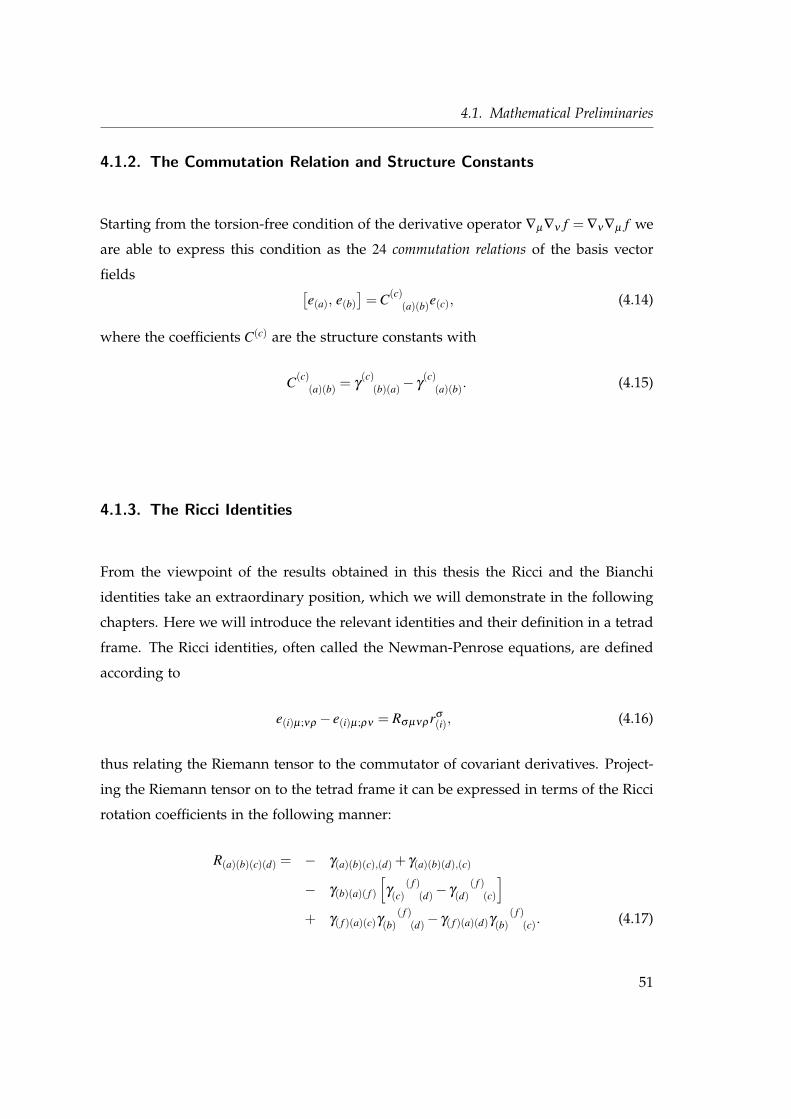
4.1. Mathematical Preliminaries
4.1.2. The Commutation Relation and Structure Constants
Starting from the torsion-free condition of the derivative operator ∇µ∇ν f = ∇ν∇µ f we
are able to express this condition as the 24 commutation relations of the basis vector
fields [e(a), e(b)
]= C(c)
(a)(b)e(c), (4.14)
where the coefficients C(c) are the structure constants with
C(c)(a)(b) = γ
(c)(b)(a)− γ
(c)(a)(b). (4.15)
4.1.3. The Ricci Identities
From the viewpoint of the results obtained in this thesis the Ricci and the Bianchi
identities take an extraordinary position, which we will demonstrate in the following
chapters. Here we will introduce the relevant identities and their definition in a tetrad
frame. The Ricci identities, often called the Newman-Penrose equations, are defined
according to
e(i)µ;νρ − e(i)µ;ρν = Rσ µνρrσ
(i), (4.16)
thus relating the Riemann tensor to the commutator of covariant derivatives. Project-
ing the Riemann tensor on to the tetrad frame it can be expressed in terms of the Ricci
rotation coefficients in the following manner:
R(a)(b)(c)(d) = − γ(a)(b)(c),(d) + γ(a)(b)(d),(c)
− γ(b)(a)( f )
[γ
( f )(c) (d)− γ
( f )(d) (c)
]+ γ( f )(a)(c)γ
( f )(b) (d)− γ( f )(a)(d)γ
( f )(b) (c). (4.17)
51
4. The Newman-Penrose Formalism
Newman and Penrose identified 18 independent non-vanishing complex components
of the Riemann tensor
R(1)(3)(1)(3), R(1)(3)(1)(4),12(R(3)(4)(1)(4)−R(1)(2)(1)(4)
), (4.18a)
R(1)(3)(1)(2), R(2)(4)(4)(1),12(R(1)(2)(1)(3)−R(3)(4)(1)(3)
), (4.18b)
R(2)(4)(3)(1), R(2)(4)(2)(1),12(R(1)(2)(1)(2)−R(3)(4)(1)(2)
), (4.18c)
R(2)(4)(4)(2), R(3)(1)(4)(3),12(R(1)(2)(3)(4)−R(3)(4)(3)(4)
), (4.18d)
R(2)(4)(4)(3), R(2)(4)(2)(3),12(R(1)(2)(3)(2)−R(2)(4)(2)(3)
), (4.18e)
R(1)(3)(3)(2), R(1)(3)(2)(4),12(R(1)(2)(4)(2)−R(3)(4)(4)(2)
), (4.18f)
and the additional complex-conjugate relations are obtained by replacing the index 3
with the index 4, and vice versa. Thus, in total we yield 36 linear independent Ricci
identities. In chapter 5 the Ricci identities will acquire the role of evolution equations
for the Weyl scalars.
4.1.4. The Bianchi Identities
Pursuing the same projection we can express the Bianchi identities
Rµν [ρσ ;τ] = 0, (4.19)
in terms of intrinsic derivatives and tetrad components, yielding
R(a)(b)[(c)(d)|( f )] =16 ∑
[(c)(d)( f )]
R(a)(b)(c)(d),( f )
−η(n)(m)
[γ(n)(a)( f )R(m)(b)(c)(d) + γ(n)(b)( f )R(a)(m)(c)(d)
+γ(n)(c)( f )R(a)(b)(m)(d) + γ(n)(d)( f )R(a)(b)(c)(m)
]. (4.20)
52
4.2. Null Tetrads and Null Frames
Due to the symmetries of the Riemann tensors only 20 linear independent equations
can be derived. Written out explicitly, a complete set is provided by the eight following
complex identities
R(1)(3)[(1)(3)|(4)] = 0, R(1)(3)[(2)(1)|(4)] = 0, (4.21a)
R(1)(3)[(1)(3)|(2)] = 0, R(1)(3)[(4)(3)|(2)] = 0, (4.21b)
R(4)(2)[(1)(3)|(4)] = 0, R(4)(2)[(2)(1)|(4)] = 0, (4.21c)
R(4)(2)[(1)(3)|(2)] = 0, R(4)(2)[(4)(3)|(2)] = 0, (4.21d)
and four real identities which follow from
η(b)(c)
(R(a)(b)−
12
η(a)(b)R)|c
= 0. (4.21e)
Again, the additional complex-conjugate relations are obtained by replacing the index
3 with the index 4, and vice versa. In chapter 5 the Bianchi identities will provide a
fundamental relation between the spin coefficients and Weyl scalars.
To summarize, the basic equations which must be satisfied in the tetrad formalism
consists of 24 commutation relations, 36 Ricci identities and 20 Bianchi identities.
4.2. Null Tetrads and Null Frames
A particularly important tetrad choice has been made by Newman and Penrose, orig-
inally based on the idea of treating general relativity in terms of spinor fields [61].
Furthermore, their choice is motivated by symmetry reasons since it is particularly
well adapted to the light-cone structure of radiation in four dimensional space-times.
The vector basis chosen is a set of four null vectors; they consist of a pair real null
vectors labeled as ` and n, completed by a pair of complex conjugate null vectors de-
noted by m and m. The two real tetrad vectors point asymptotically radially inward
and radially outward whereas the complex vectors are defined on a 2-sphere. The null
53
4. The Newman-Penrose Formalism
tetrad satisfies the orthogonality condition
` ·m = ` · m = n ·m = n · m = 0, (4.22a)
besides the requirements that the vectors be null
` · ` = n ·n = m ·m = m · m = 0. (4.22b)
Additionally they satisfy the normalization conditions
` ·n = 1, (4.22c)
m · m = −1, (4.22d)
where this is not an essential requirement and may be dropped. Imposing these
conditions the matrix η in Eq. (4.3) takes the form
ηµν =
0 1 0 0
1 0 0 0
0 0 0 −1
0 0 −1 0
. (4.23)
By utilizing the definition of the tetrad introduced in Eq. (4.1) to Eq. (4.3) we can
deduce the following correspondence between the tetrad vectors and null vectors
e(1) = e(2) = n; e(2) = e(1) = l, (4.24a)
e(3) =−e(4) =−m; e(4) =−e(3) =−m. (4.24b)
In this notation the metric tensor gµν of the 4-dimensional space-time takes the form
gµν = `µnν +nµ`ν −mµmν − mµmν = 2`(µnν)−2m(µmν), (4.25)
54
4.3. Spin Coefficients
and the inverse is defined accordingly
gµν = 2`(µnν)−2m(µmν). (4.26)
4.3. Spin Coefficients
The 24 Ricci rotation-coefficients γ(a)(b)(c) introduced in 4.1.1 are now 12 complex quan-
tities and called spin coefficients, designated by a special notation:
κ = γ(3)(1)(1); ρ = γ(3)(1)(4); ε =12(γ(2)(1)(1) + γ(3)(4)(1)
); (4.27a)
σ = γ(3)(1)(3); µ = γ(2)(4)(3); γ =12(γ(2)(1)(2) + γ(3)(4)(2)
); (4.27b)
λ = γ(2)(4)(4); τ = γ(3)(1)(2); α =12(γ(2)(1)(4) + γ(3)(4)(4)
); (4.27c)
ν = γ(2)(4)(2); π = γ(2)(4)(1); β =12(γ(2)(1)(3) + γ(3)(4)(3)
). (4.27d)
An equivalent formulation in terms of tetrad components is
κ = mµ`ν∇ν`µ , ν = nµnν
∇νmµ , (4.28a)
σ = mµmν∇ν`µ , λ = nµmν
∇νmµ , (4.28b)
ρ = mµmν∇ν`µ , µ = nµmν
∇νmµ , (4.28c)
τ = mµnν∇ν`µ , π = nµ`ν
∇νmµ , (4.28d)
ε =12`ν(nµ
∇ν`µ +mµ∇νmµ
), (4.28e)
γ =12
nν(nµ
∇ν`µ +mµ∇νmµ
), (4.28f)
α =12
mν(nµ
∇ν`µ +mµ∇νmµ
), (4.28g)
β =12
mν(nµ
∇ν`µ +mµ∇νmµ
). (4.28h)
We want to stress here an important property related to the `↔ n exchange trans-
formation. If we exchange the two real null vectors, then the spin coefficients become
55
4. The Newman-Penrose Formalism
interchanged as follows
κ ↔−ν∗, ρ ↔−µ∗, σ ↔−λ ∗, (4.29a)
α ↔−β ∗, ε ↔−γ∗, π ↔−τ∗. (4.29b)
The spin coefficients can be related to physical properties of the tetrad vectors consti-
tuting the tetrad; utilizing the exchange operation we can immediately conclude that
the physical property which connects (κ,ρ,σ ,α,ε,π) to the null vector ` is the same
that relates (ν ,µ,λ ,β ,γ,τ) to the n vector. Therefore we can restrict our attention to
the physical meaning of the spin coefficients which are related to the ` vector.
Assuming space-time contains a ray congruence (i.e. a foliation by null geodesics)
that is singled out, we can relate the spin coefficients to the ` vector in the following
manner:
• The null vector `µ may be chosen to point in the direction of the rays, whose
geodicity can be stated as κ = 0.
• Affine normalization, i.e. parallel propagation of `µ , is stated as ε + ε = 0.
• ρ as the “complex divergence”, defined as ρ = 12
(−∇µ`µ + i
√∇[µ `ν ]∇
[µ `ν ])
.
• σ measures the shear of the null congruence of geodesics dened by
σσ = 12
(∇(µ `ν)∇
(µ `ν)− 12
(∇µ`µ
)2)
.
• When the ray congruence is a gradient field, i.e. `µ = ∇µΦ, then τ = α +β .
For a detailed derivation of such properties we suggest a very good textbook by Pen-
rose and Rindler [62].
4.4. Weyl Tensor and Weyl Scalars
In addition to the spin coefficients the most relevant quantities in the Newman-Penrose
formalism are the Weyl scalars, which comprise all the important information about
56
4.4. Weyl Tensor and Weyl Scalars
the space-time under consideration. They are given by the contraction of the confor-
mal Weyl tensor over a specific combination of the null tetrad (`µ ,nµ ,mµ , mµ). Since
Weyl scalars are true scalars the choice of the coordinate system is irrelevant for their
calculation; however, they do depend on the tetrad choice which constitutes the gauge
freedom in this formalism.
But before we move to the calculation of these quantities we need to define the
conformal Weyl tensor. It comprises of the conformally invariant part of the Riemann
tensor, thus we introduce the Weyl tensor as the trace-free part of the Riemann tensor:
Cµνρσ = Rµνρσ −1
(n−2)(gµρRνσ +gνσ Rµρ −gνρRµσ −gµσ Rνρ
)+
1(n−1)(n−2)
(gµρ gνσ − gµσ gνρ
)R. (4.30)
It is a straightforward to show that the Weyl tensor possesses the same symmetries as
the curvature tensor, namely
Cµνρσ =−Cµνσρ =−Cνµρσ = Cρσ µν , (4.31a)
Cµνρσ +Cµσνρ +Cµρσν = 0, (4.31b)
with the additional symmetry gρµ Cµνρσ = 0. Secondly, to determine the Weyl tensor
on a manifold, a connection and a metric must be defined.
Projecting the Weyl tensor on to the tetrad frame, we have in 4 dimensions
C(a)(b)(c)(d) = R(a)(b)(c)(d)−12(η(a)(c)R(b)(d) +η(b)(d)R(a)(c)−η(b)(c)R(a)(d)−η(a)(d)R(b)(c)
)+
16(η(a)(c)η(b)(d) − η(a)(d)η(b)(c)
)R, (4.32)
where now we are raising and lowering quantities with ηµν instead of gµν .
A detailed analysis of the Weyl tensor shows that it has 10 degrees of freedom,
which we can express by introducing five complex self-dual scalar quantities, the Weyl
57
4. The Newman-Penrose Formalism
scalars:
Ψ0 = −C(1)(3)(1)(3) = −Cαβγδ lα mβ lγ mδ , (4.33a)
Ψ1 = −C(1)(2)(1)(3) = −Cαβγδ lα nβ lγ mδ , (4.33b)
Ψ2 = −C(1)(3)(4)(2) = −Cαβγδ lα mβ mγ nδ , (4.33c)
Ψ3 = −C(1)(2)(4)(2) = −Cαβγδ lα nβ mγ nδ , (4.33d)
Ψ4 = −C(2)(4)(2)(4) = −Cαβγδ nα mβ nγ mδ . (4.33e)
However, it is important to stress that the Weyl scalars still possess the inherit degrees
of freedom of general relativity, even if the quantities do not depend on the coordinates
any more. We can perform so-called tetrad rotations to change the value of the Weyl
scalars. We will clarify these issues in the remaining part of the chapter.
4.5. Curvature Invariants
Still, it is possible to define quantities in the Newman-Penrose formalism which nei-
ther depend on the coordinate, nor are subject to tetrad transformations. Two well-
known complex curvature invariants are (commonly) defined by
I =116(C ρσ
µν C µν
ρσ − iC ρσ
µν C µν
ρσ
), (4.34a)
J =196
(C ρσ
µν C µν
ρσ C µν
αβ− iC ρσ
µν C αβ
ρσ C µν
αβ
), (4.34b)
where C µν
ρσ = 12 ε
αβ
ρσ C µν
αβis the Hodge dual of the Weyl tensor C µν
ρσ . The scalars
are also often called Kretschmann invariants after Erich Kretschmann [63]. They are
essentially the square and cube of the self-dual part, C ρσ
µν = C ρσ
µν + i2 ε
αβ
µν C ρσ
αβ, of
the Weyl tensor:
I = CµνρσCµνρσ , (4.35a)
J = CµνρσCρσ
αβCαβ µν . (4.35b)
58
4.6. Tetrad Transformations
We may re-express the curvature invariants in terms of Weyl scalars as
I = 3Ψ22 +Ψ4Ψ0−4Ψ1Ψ3, (4.36a)
J = −Ψ32 +2Ψ1Ψ2Ψ3−Ψ0Ψ
33−Ψ
21Ψ4 +Ψ0Ψ2Ψ4. (4.36b)
Additionally, we define the speciality index S in terms of curvature invariants
S =27J2
I3 , (4.37)
which plays an important role in the Petrov classification in section 4.7.
4.6. Tetrad Transformations
As mentioned in section 4.4 and section 4.5, Weyl scalars are not tetrad invariant in
contrast to the curvature invariants. They are subject to transformations which we
classify in this section. We can perform a Lorentz transformation at some point and
extend it continuously through all of space-time.
The six degrees of freedom of the group of Lorentz transformations correspond to
the following tetrad rotations in the Newman-Penrose formalism, which preserve the
underlying orthogonality and normalization conditions:
• Type I `→ `; n→ n+a∗m+am+aa∗`; m→ m+a`; m→ m+a∗`,
• Type II n→ n; `→ `+b∗m+bm+bb∗n; m→ m+bn; m→ m+b∗n,
• Type III `→ |B|−1`; n→ |B|n; m→ eiΘm; m→ e−iΘm.
Here a and b are two complex functions. The spin-boost parameter B is defined as
B = Ae−iΘ, where the modulus A and the phase Θ of the complex valued boost read
A =√
ℜ [B]2 +ℑ [B]2, (4.38a)
Θ = arctan(
ℑ [B]ℜ [B]
). (4.38b)
59
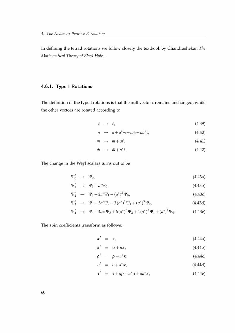
4. The Newman-Penrose Formalism
In defining the tetrad rotations we follow closely the textbook by Chandrashekar, The
Mathematical Theory of Black Holes.
4.6.1. Type I Rotations
The definition of the type I rotations is that the null vector ` remains unchanged, while
the other vectors are rotated according to
` → `, (4.39)
n → n+a∗m+am+aa∗`, (4.40)
m → m+a`, (4.41)
m → m+a∗`. (4.42)
The change in the Weyl scalars turns out to be
ΨI0 → Ψ0, (4.43a)
ΨI1 → Ψ1 +a∗Ψ0, (4.43b)
ΨI2 → Ψ2 +2a∗Ψ1 +(a∗)2
Ψ0, (4.43c)
ΨI3 → Ψ3 +3a∗Ψ2 +3(a∗)2
Ψ1 +(a∗)3Ψ0, (4.43d)
ΨI4 → Ψ4 +4a∗Ψ3 +6(a∗)2
Ψ2 +4(a∗)3Ψ1 +(a∗)4
Ψ0. (4.43e)
The spin coefficients transform as follows:
κI = κ, (4.44a)
σI = σ +aκ, (4.44b)
ρI = ρ +a∗κ, (4.44c)
εI = ε +a∗κ, (4.44d)
τI = τ +aρ +a∗σ +aa∗κ, (4.44e)
60
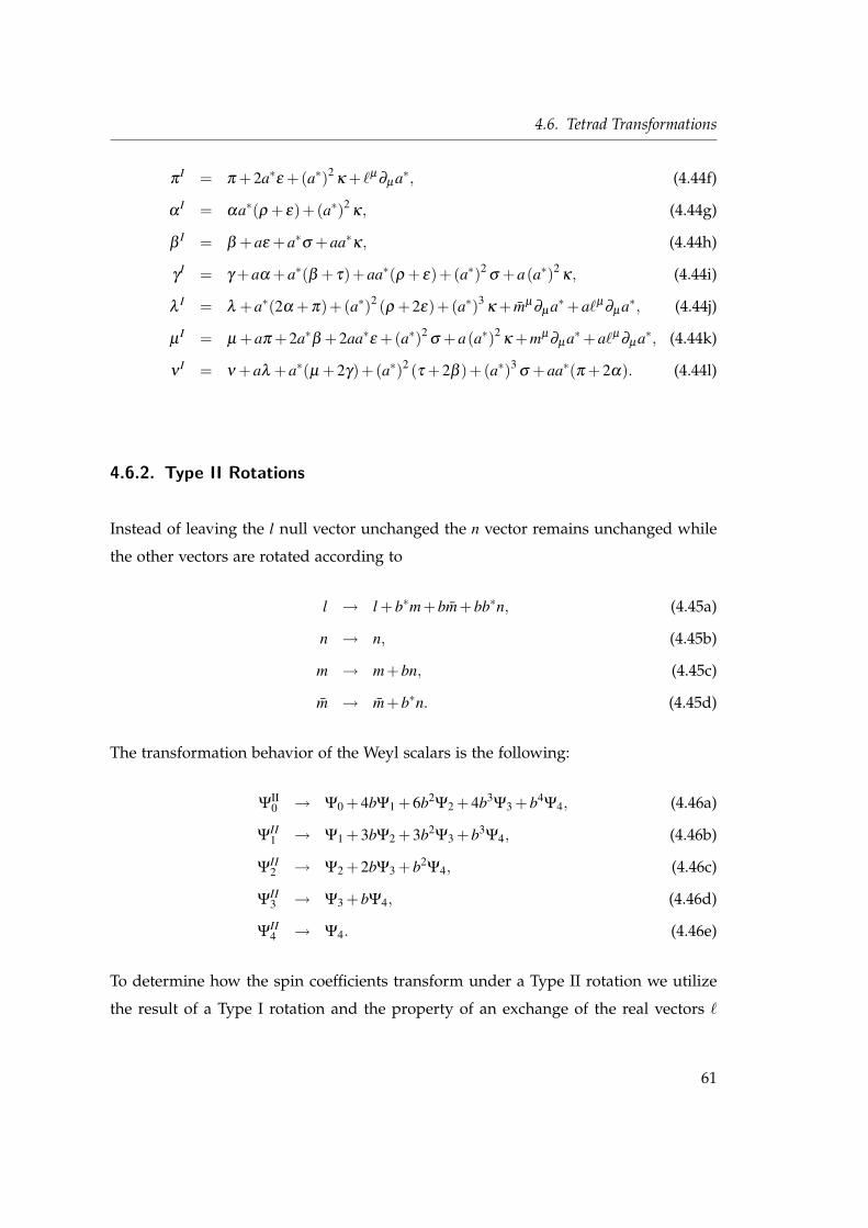
4.6. Tetrad Transformations
πI = π +2a∗ε +(a∗)2
κ + `µ∂µa∗, (4.44f)
αI = αa∗(ρ + ε)+(a∗)2
κ, (4.44g)
βI = β +aε +a∗σ +aa∗κ, (4.44h)
γI = γ +aα +a∗(β + τ)+aa∗(ρ + ε)+(a∗)2
σ +a(a∗)2κ, (4.44i)
λI = λ +a∗(2α +π)+(a∗)2 (ρ +2ε)+(a∗)3
κ + mµ∂µa∗+a`µ
∂µa∗, (4.44j)
µI = µ +aπ +2a∗β +2aa∗ε +(a∗)2
σ +a(a∗)2κ +mµ
∂µa∗+a`µ∂µa∗, (4.44k)
νI = ν +aλ +a∗(µ +2γ)+(a∗)2 (τ +2β )+(a∗)3
σ +aa∗(π +2α). (4.44l)
4.6.2. Type II Rotations
Instead of leaving the l null vector unchanged the n vector remains unchanged while
the other vectors are rotated according to
l → l +b∗m+bm+bb∗n, (4.45a)
n → n, (4.45b)
m → m+bn, (4.45c)
m → m+b∗n. (4.45d)
The transformation behavior of the Weyl scalars is the following:
ΨII0 → Ψ0 +4bΨ1 +6b2
Ψ2 +4b3Ψ3 +b4
Ψ4, (4.46a)
ΨII1 → Ψ1 +3bΨ2 +3b2
Ψ3 +b3Ψ4, (4.46b)
ΨII2 → Ψ2 +2bΨ3 +b2
Ψ4, (4.46c)
ΨII3 → Ψ3 +bΨ4, (4.46d)
ΨII4 → Ψ4. (4.46e)
To determine how the spin coefficients transform under a Type II rotation we utilize
the result of a Type I rotation and the property of an exchange of the real vectors `
61
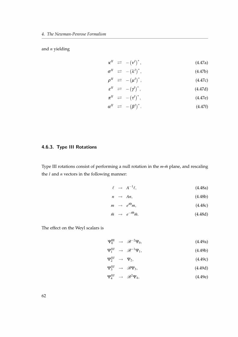
4. The Newman-Penrose Formalism
and n yielding
κII −
(ν
I)∗ , (4.47a)
σII −
(λ
I)∗ , (4.47b)
ρII −
(µ
I)∗ , (4.47c)
εII −
(γ
I)∗ , (4.47d)
πII −
(τ
I)∗ , (4.47e)
αII −
(β
I)∗ . (4.47f)
4.6.3. Type III Rotations
Type III rotations consist of performing a null rotation in the m-m plane, and rescaling
the l and n vectors in the following manner:
` → A−1`, (4.48a)
n → An, (4.48b)
m → eiΘm, (4.48c)
m → e−iΘm. (4.48d)
The effect on the Weyl scalars is
ΨIII0 → B−2
Ψ0, (4.49a)
ΨIII1 → B−1
Ψ1, (4.49b)
ΨIII2 → Ψ2, (4.49c)
ΨIII3 → BΨ3, (4.49d)
ΨIII4 → B2
Ψ4, (4.49e)
62
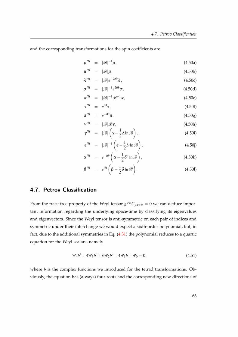
4.7. Petrov Classification
and the corresponding transformations for the spin coefficients are
ρIII = |B|−1
ρ, (4.50a)
µIII = |B|µ, (4.50b)
λIII = |B|e−2iΘ
λ , (4.50c)
σIII = |B|−1e2iΘ
σ , (4.50d)
κIII = |B|−1B−1
κ, (4.50e)
τIII = eiΘ
τ, (4.50f)
πIII = e−iΘ
π, (4.50g)
νIII = |B|Bν , (4.50h)
γIII = |B|
(γ− 1
2∆ lnB
), (4.50i)
εIII = |B|−1
(ε− 1
2D lnB
), (4.50j)
αIII = e−iΘ
(α− 1
2δ∗ lnB
), (4.50k)
βIII = eiΘ
(β − 1
2δ lnB
). (4.50l)
4.7. Petrov Classification
From the trace-free property of the Weyl tensor gρµ Cµνρσ = 0 we can deduce impor-
tant information regarding the underlying space-time by classifying its eigenvalues
and eigenvectors. Since the Weyl tensor is anti-symmetric on each pair of indices and
symmetric under their interchange we would expect a sixth-order polynomial, but, in
fact, due to the additional symmetries in Eq. (4.31) the polynomial reduces to a quartic
equation for the Weyl scalars, namely
Ψ4b4 +4Ψ3b3 +6Ψ2b2 +4Ψ1b+Ψ0 = 0, (4.51)
where b is the complex functions we introduced for the tetrad transformations. Ob-
viously, the equation has (always) four roots and the corresponding new directions of
63
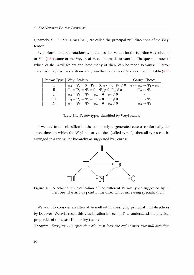
4. The Newman-Penrose Formalism
`, namely, `→ `+b∗m +bm +bb∗n, are called the principal null-directions of the Weyl
tensor.
By performing tetrad rotations with the possible values for the function b as solution
of Eq. (4.51) some of the Weyl scalars can be made to vanish. The question now is
which of the Weyl scalars and how many of them can be made to vanish. Petrov
classified the possible solutions and gave them a name or type as shown in Table (4.1).
Petrov Type Weyl Scalars Gauge ChoiceI Ψ0 = Ψ4 = 0 Ψ1 6= 0, Ψ2 6= 0, Ψ3 6= 0 Ψ0∧Ψ4↔Ψ1∧Ψ3
II Ψ1 = Ψ3 = Ψ4 = 0 Ψ0 6= 0, Ψ2 6= 0 Ψ0↔Ψ4
D Ψ0 = Ψ1 = Ψ3 = Ψ4 = 0 Ψ2 6= 0 -III Ψ0 = Ψ2 = Ψ3 = Ψ4 = 0 Ψ1 6= 0 Ψ1↔Ψ3
N Ψ1 = Ψ2 = Ψ3 = Ψ4 = 0 Ψ0 6= 0 Ψ0↔Ψ4
Table 4.1.: Petrov types classified by Weyl scalars
If we add to this classification the completely degenerated case of conformally flat
space-times in which the Weyl tensor vanishes (called type 0), then all types can be
arranged in a triangular hierarchy as suggested by Penrose.
Figure 4.1.: A schematic classification of the different Petrov types suggested by R.Penrose. The arrows point in the direction of increasing specialization.
We want to consider an alternative method in classifying principal null directions
by Debever. We will recall this classification in section () to understand the physical
properties of the quasi-Kinnersley frame:
Theorem: Every vacuum space-time admits at least one and at most four null directions
64
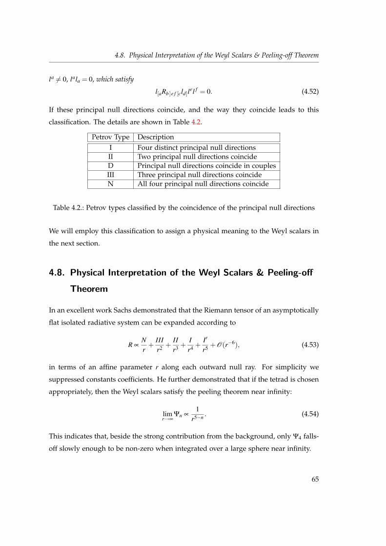
4.8. Physical Interpretation of the Weyl Scalars & Peeling-off Theorem
la 6= 0, lala = 0, which satisfy
l[aRb ]e f [cld]lel f = 0. (4.52)
If these principal null directions coincide, and the way they coincide leads to this
classification. The details are shown in Table 4.2.
Petrov Type DescriptionI Four distinct principal null directionsII Two principal null directions coincideD Principal null directions coincide in couplesIII Three principal null directions coincideN All four principal null directions coincide
Table 4.2.: Petrov types classified by the coincidence of the principal null directions
We will employ this classification to assign a physical meaning to the Weyl scalars in
the next section.
4.8. Physical Interpretation of the Weyl Scalars & Peeling-off
Theorem
In an excellent work Sachs demonstrated that the Riemann tensor of an asymptotically
flat isolated radiative system can be expanded according to
R ∝Nr
+IIIr2 +
IIr3 +
Ir4 +
I′
r5 +O(r−6), (4.53)
in terms of an affine parameter r along each outward null ray. For simplicity we
suppressed constants coefficients. He further demonstrated that if the tetrad is chosen
appropriately, then the Weyl scalars satisfy the peeling theorem near infinity:
limr→∞
Ψn ∝1
r5−n . (4.54)
This indicates that, beside the strong contribution from the background, only Ψ4 falls-
off slowly enough to be non-zero when integrated over a large sphere near infinity.
65
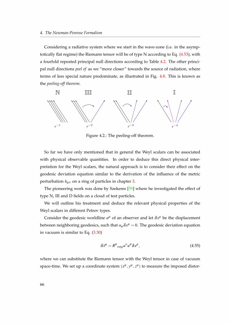
4. The Newman-Penrose Formalism
Considering a radiative system where we start in the wave-zone (i.e. in the asymp-
totically flat regime) the Riemann tensor will be of type N according to Eq. (4.53), with
a fourfold repeated principal null directions according to Table 4.2. The other princi-
pal null directions peel of as we “move closer” towards the source of radiation, where
terms of less special nature predominate, as illustrated in Fig. 4.8. This is known as
the peeling-off theorem.
Figure 4.2.: The peeling-off theorem.
So far we have only mentioned that in general the Weyl scalars can be associated
with physical observable quantities. In order to deduce this direct physical inter-
pretation for the Weyl scalars, the natural approach is to consider their effect on the
geodesic deviation equation similar to the derivation of the influence of the metric
perturbation hµν on a ring of particles in chapter 3.
The pioneering work was done by Szekeres [59] where he investigated the effect of
type N, III and D fields on a cloud of test particles.
We will outline his treatment and deduce the relevant physical properties of the
Weyl scalars in different Petrov types.
Consider the geodesic worldline uµ of an observer and let δxµ be the displacement
between neighboring geodesics, such that uµδxµ = 0. The geodesic deviation equation
in vacuum is similar to Eq. (3.30)
δ xµ = Rµ
νσρuνuσδxρ , (4.55)
where we can substitute the Riemann tensor with the Weyl tensor in case of vacuum
space-time. We set up a coordinate system (xµ , yµ , zµ) to measure the imposed distor-
66
4.8. Physical Interpretation of the Weyl Scalars & Peeling-off Theorem
tion on a ring of particles by the Weyl scalars in three dimensional space.
4.8.1. Petrov Type N
As outlined in the last section we end up having only Ψ0 (or Ψ4) non-zero in the most
specialized Petrov type by making use of the tetrad rotations, see table 4.1. In this
particular case the geodesic deviation equation (4.55) reads according to Szekeres [59]
δ xµ = Ψ0 [(xµxν − yµyν)− i(xνyµ − xµyν)]δxν , (4.56)
and considering only the real part we end up with
δ xµ = [ℜ(Ψ0)(xµxν − yµyν)+ℑ(Ψ0)(xνyµ − xµyν)]δxν . (4.57)
Since we have only performed type I and type II rotations so far we can make use of the
remaining degree of freedom related to type III tetrad rotations to set the imaginary
part ℑ(Ψ0) to zero, yielding
δ xµ = ℜ(Ψ0)(xµxν − yµyν)δxν . (4.58)
The resulting force on a ring of test particles located at z = 0 turns out being a trans-
verse distortion. Szekeres terms this a pure transverse gravitational wave. This holds
for Ψ0 as well as for Ψ4.
4.8.2. Petrov Type III
For a type III space-time all scalars vanish except Ψ3 (or Ψ1), see table 4.1. Szekeres
demonstrated that the geodesic equation reads
δ xµ = Ψ1 [(zµxν + xµzν)− i(zνyµ + yµzν)]δxν . (4.59)
As in case of Petrov type N we can utilize spin transformations to set ℑ(Ψ1) = 0, thus
ending up with
δ xµ = ℜ(Ψ1)(zµxν + xµzν)δxν . (4.60)
67
4. The Newman-Penrose Formalism
Obviously, the effect on the ring of test particles located at z = 0 in type III is still planar,
but the wave contains a longitudinal directional contribution, i.e. along zµ . Thus the
two scalars Ψ1 and Ψ3 possess a longitudinal contribution which is the reason Szekeres
terms this a longitudinal wave component.
4.8.3. Petrov Type D
Here the only non-vanishing Weyl scalar is Ψ2 (table 4.1). The geodesic deviation
equation turns out as
δ xµ = Ψ2
[zµzν −
12
(xµyν − yµxν)]
δxν . (4.61)
The force on a ring of test particles results in a distortion to an ellipsoid with major
contribution in the orthogonal direction. We will demonstrate in section 4.12 that an
isolated black hole space-time is exactly Petrov type D. Furthermore, since Ψ2 is the
only non-vanishing scalar in type D it can be shown that the tidal force action on a
radially in-falling observer can be calculated according to Eq. (4.61) in a Schwarzschild
space-time. Szekeres terms this a Coulomb-type field.
4.8.4. Petrov Type II
According to the classification by Petrov the non-vanishing scalars for a type II field
are Ψ2 and Ψ0 (or Ψ4). Employing the results we have obtained for Petrov type D and
type N we can relate Ψ2 to the Coulomb-type contribution and Ψ0 gives a transverse
contribution, namely
δ xµ = [ℜ(Ψ0)(xµxν − yµyν)−ℑ(Ψ0)(xνyµ + xµyν)]δxν , (4.62)
where we perform a type III rotation to set ℑ(Ψ0) = 0. Thus the Weyl scalars in type
II space-time are related to a superposition of a Coulomb-type field (Ψ2) and a radiative
wave component (Ψ0).
68
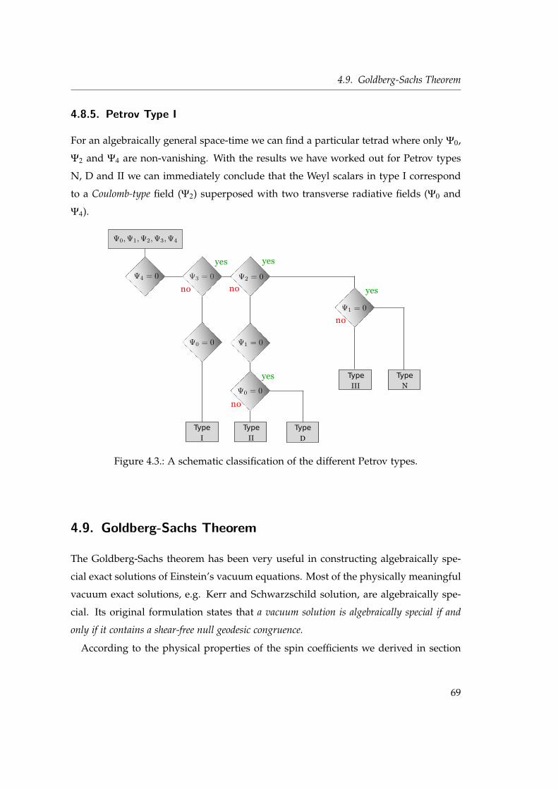
4.9. Goldberg-Sachs Theorem
4.8.5. Petrov Type I
For an algebraically general space-time we can find a particular tetrad where only Ψ0,
Ψ2 and Ψ4 are non-vanishing. With the results we have worked out for Petrov types
N, D and II we can immediately conclude that the Weyl scalars in type I correspond
to a Coulomb-type field (Ψ2) superposed with two transverse radiative fields (Ψ0 and
Ψ4).
yes
no
NIII
DIII
TypeType
TypeTypeType
no
yes
no
no
yes
yes
Figure 4.3.: A schematic classification of the different Petrov types.
4.9. Goldberg-Sachs Theorem
The Goldberg-Sachs theorem has been very useful in constructing algebraically spe-
cial exact solutions of Einstein’s vacuum equations. Most of the physically meaningful
vacuum exact solutions, e.g. Kerr and Schwarzschild solution, are algebraically spe-
cial. Its original formulation states that a vacuum solution is algebraically special if and
only if it contains a shear-free null geodesic congruence.
According to the physical properties of the spin coefficients we derived in section
69
4. The Newman-Penrose Formalism
4.3, we can reformulate this statement to deduce the consequences of the Goldberg-
Sachs theorem for the Weyl scalars and spin coefficients in the Newman-Penrose for-
malism. The proof of the theorem can be found in [64].
If a space-time is of Petrov type II and a null basis is chosen such that l is the repeated null
direction and so Ψ0 = Ψ1 = 0, then the two spin coefficients κ and σ are vanishing; conversely
if κ = σ = 0 the Ψ0 = Ψ1 = 0 and the space-time is of Petrov type II.
A consequence of this, which is commonly referred to as the Goldberg-Sachs theo-
rem, states that
Theorem 1 If a space-time is of Petrov type D and a null basis is chosen such that l is
one repeated null direction and n is the other one, such that Ψ0 = Ψ1 = Ψ3 = Ψ4 = 0, then
the spin coefficients κ , σ , ν and λ are vanishing; conversely if κ = σ = ν = λ = 0 then
Ψ0 = Ψ1 = Ψ3 = Ψ4 = 0 and the space-time is of Petrov type D.
4.10. Bondi Frame
The calculations of gravitational radiation at future null infinity are based on the foun-
dational works of Bondi [65] and Sachs [17] and have led to the extremely important
conclusion that a gravitationally radiating system loses mass, and further to the iden-
tification of the Bondi-Metzner-Sachs asymptotic symmetry group [12, 11, 66, 67, 62,
65, 17]. The detailed derivation of these important but highly complex results goes
beyond the scope of this work. Therefore we will only present the key results.
The identification of the Bondi frame relies upon the identification of a family of
null surfaces labeled by a retarded time-coordinate u. In flat space-time a suitable
family might be the null cones emanating from a time-like world line. Each of these
surfaces is generated by a two-parameter family of null geodesics each labeled by
sphere coordinates (θ ,φ) or equivalently by complex stereographic coordinates(ζ , ζ
),
where ζ = eiφ cot(θ/2). The “length” along the geodesics is given by the affine “ra-
dial” parameter r. In summary, in the standard literature a null coordinate system is
70
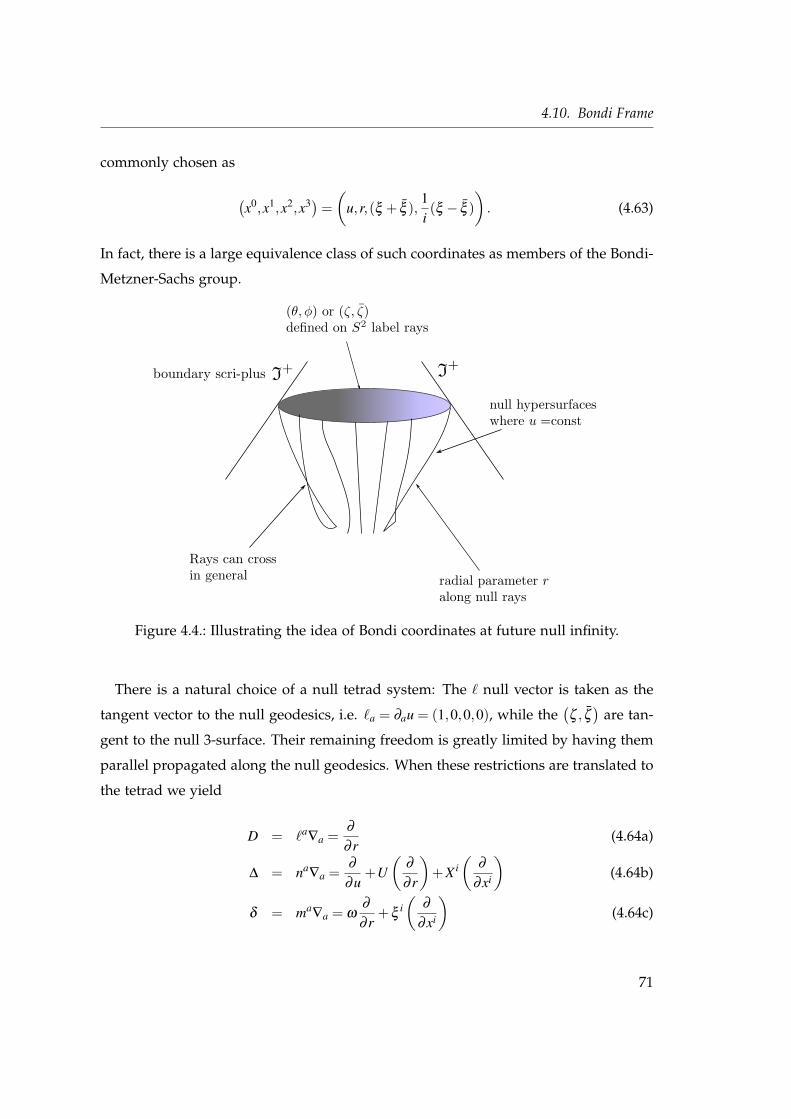
4.10. Bondi Frame
commonly chosen as
(x0,x1,x2,x3)=
(u,r,(ξ + ξ ),
1i(ξ − ξ )
). (4.63)
In fact, there is a large equivalence class of such coordinates as members of the Bondi-
Metzner-Sachs group.
Figure 4.4.: Illustrating the idea of Bondi coordinates at future null infinity.
There is a natural choice of a null tetrad system: The ` null vector is taken as the
tangent vector to the null geodesics, i.e. `a = ∂au = (1,0,0,0), while the(ζ , ζ
)are tan-
gent to the null 3-surface. Their remaining freedom is greatly limited by having them
parallel propagated along the null geodesics. When these restrictions are translated to
the tetrad we yield
D = `a∇a =
∂
∂ r(4.64a)
∆ = na∇a =
∂
∂u+U
(∂
∂ r
)+X i
(∂
∂xi
)(4.64b)
δ = ma∇a = ω
∂
∂ r+ξ
i(
∂
∂xi
)(4.64c)
71

4. The Newman-Penrose Formalism
where X i =(x3,x4
)=(ζ , ζ
). ξ i, U and ω are arbitrary functions of the coordinates
constituting the metric according to
g22 = 2(U−ωω) , (4.65)
g2A = XA−(ωζ
A +ωζA) , (4.66)
gAB = −(ζ
Aζ
B +ζAζ
B) . (4.67)
Keeping (ξ = const) and (ξ = const) on the null hypersurface u = const, one moves
along a null direction by increasing r.
4.11. Kinnersley Tetrad
A particular null frame in the Newman-Penrose formalism is constructed by making
the following definition [16]:
Def. 1 A Kinnersley frame for a type D space-time is a frame where the two real tetrad null
vectors coincide with the two repeated principal null directions of the Weyl tensor.
These conditions fix 4 of 6 degrees of freedom of the Lorentz group corresponding
to type I and type II rotations.
Kinnersley enforced the additional condition ε = 0 to single out a particular tetrad,
commonly known as the Kinnersley tetrad. The motivation for his choice is presum-
ably related to the physical properties of the ` null vector: the geodesic equation for `
reads
`µ∇µ`ν = (ε + ε
∗)`ν −κmν −κ∗mν , (4.68)
which shows that if the two spin coefficients κ and ε vanish, the vector `µ is geodesic
and affinely parametrized.
In the limit of type D the Goldberg-Sachs theorem (cf. section 4.9) guarantees that
κ = 0, so the additional condition ε = 0 enforces the affine parameterization of `µ .
72
4.12. Black Hole Space-Times in the NP Formalism
In the Kinnersley tetrad all scalars vanish except Ψ2, i.e. it is a canonical frame [68]
for Petrov type D, thus the speciality index S in Eq. (4.37) reduces to
S→27(−Ψ3
2
)2(3Ψ2
2
)3 = 1. (4.69)
4.12. Black Hole Space-Times in the NP Formalism
As an example of the Newman-Penrose formalism we calculate all relevant quantities
of the Kerr solution. Since we expect every distorted black hole to relax to the Kerr
(Schwarzschild) solution it plays a crucial role as the final state in every black hole
simulation1. We start by defining the real null vectors ` and n in terms of radial null
geodesics and adjoin orthogonally to them the complex conjugated null vector pair
(m, m), yielding
`µ =1∆
(r2 +a2,∆,0,a
), (4.70a)
nµ =1
2Σ
(r2 +a2,−∆,0,a
), (4.70b)
mµ =1√2Σ
(iasinθ ,0,1, icosecθ) , (4.70c)
where Σ = r2 + a2 cos2 θ and Σ = r + iacosθ . Such a tetrad still satisfies the null vector
conditions in Eqs. (4.22). We calculate the spin coefficients according to Eqs. (4.28)
yielding
ρ = − 1r− iacosθ
, β =− cotθ
2√
2Σ, (4.71)
π =iasinθ
Σ√
2, τ =− iasinθ
Σ√
2, (4.72)
µ = − ∆
2ΣΣ, γ = µ +
r−M2Σ
, (4.73)
α = π−β , κ = σ = ν = λ = 0. (4.74)
1This can be regarded as a consequence of Birkhoff’s theorem in general relativity [69].
73
4. The Newman-Penrose Formalism
In agreement with the Goldberg-Sachs theorem in section 4.9 we find that the spin
coefficients κ,σ ,ν ,λ vanish, leading us to the conclusion that the Kerr space-time is
Petrov type D. Secondly, we can conclude that the only non-vanishing Weyl scalar is
Ψ2. Evaluating the Weyl scalars yields the expected result that
Ψ0 = Ψ1 = Ψ3 = Ψ4 = 0, (4.75)
and Ψ2 reads
(Ψ2)K =− M
(r− iacosθ)3 . (4.76)
As usual in the limit of vanishing rotation, a→ 0, we recover the Schwarzschild solu-
tion.
4.13. Perturbation Approach in the NP Formalism
After introducing the basic concepts of the Newman-Penrose formalism in the for-
going sections we are now able to continue our analysis of black hole perturbations
by presenting Teukolsky’s results for the Kerr space-time. In addition, we will be
able to enhance our understanding of the physical meaning of the Weyl scalars in the
wave-zone within perturbation theory.
The perturbation equation for Schwarzschild (cf. Bardeen-Press equation [14]) can
be easily recovered from Teukolsky’s solution by letting the rotation parameter a go
to zero. The problem is of considerable complexity; therefore we will only outline
the vacuum solution and refer to the original paper by Teukolsky [15] for a detailed
description.
4.13.1. The Perturbation Equations
The first step in Teukolsky’s analysis is to consider a type D space-time, i.e. an iso-
lated (Kerr) black hole which will be gravitationally perturbed later on. We start our
analysis by defining a tetrad for wave-extraction where we can connect the transverse
74
4.13. Perturbation Approach in the NP Formalism
gravitational radiation with the Weyl scalars Ψ0 and Ψ4. As described in section 4.7
and section 4.8, a well-suited tetrad for such a task is the Kinnersley tetrad, where we
know from the Goldberg-Sachs theorem that
Ψ0 = Ψ1 = Ψ3 = Ψ4 = 0; Ψ2 6= 0; (4.77a)
κ = σ = ν = λ = 0; ρ,µ,τ,π,γ,β ,α 6= 0. (4.77b)
Teukolsky managed to combine the non-vanishing Bianchi identities and Ricci identi-
ties (cf. section 4.1) for the first-order perturbation of the radiation scalars ΨP0 and ΨP
4
in such a way that he yielded the following two decoupled equations:
[(D−3ε + ε∗−4ρ−ρ
∗)(∆−4γ + µ) −
(δ +π∗−α
∗−3β −4τ)(δ ∗+π−4α)−3ΨB2
]Ψ
P0 = 0 (4.78a)
[(D−3ε + ε∗−4ρ−ρ
∗)(∆−4γ + µ) −
(δ +π∗−α
∗−3β −4τ)(δ ∗+π−4α)−3ΨB2
]Ψ
P4 = 0 (4.78b)
where D, ∆, δ and δ ∗ are the usual directional derivatives defined in Eqs. (4.8)
D = lµ∇µ , ∆ = nµ
∇µ , δ = mµ∇µ , δ
∗ = mµ∇µ . (4.79)
These two decoupled equations (4.78a, 4.78b) carry all non-trivial features of the space-
time, i.e. they describe to linear order the dynamics of a gravitationally perturbed Kerr
black hole.
4.13.2. Teukolsky Master equation
The next step is to write out the equations in a particular coordinate system. We make
use of pseudo-spherical coordinates (Boyer-Lindquist coordinates), where the metric
of a Kerr black hole reads
ds2 =(
1− 2MrΣ
)dt2 +
(4M ar sin2
θ
Σ
)dtdφ − Σ
∆dr2−Σdθ
2− sin2θ
(∆
Σ
)dφ
2, (4.80)
75
4. The Newman-Penrose Formalism
with Σ = r2 +a2 cos2 θ , ∆ = r2−2M r +a2, ∆ = r2 +a2 +2M ar sin2θ , M is the mass of the
black hole and Ma its angular momentum. The Kinnersley tetrad of a Kerr space-time
in pseudo-spherical coordinates reads
`µ =1∆
(r2 +a2,∆,0,a
), (4.81a)
nµ =1
2Σ
(r2 +a2,−∆,0,a
), (4.81b)
mµ =1√2Σ
(iasinθ ,0,1, icosecθ) . (4.81c)
The non-vanishing spin coefficients, which can be derived by using their definitions
in Eq. (4.28), turn out as
ρ = − 1r− iacosθ
, β =− cotθ
2√
2Σ, (4.82a)
π =iasinθ
Σ√
2, τ =− iasinθ
Σ√
2, (4.82b)
µ = − ∆
2ΣΣ, γ = µ +
r−M2Σ
, (4.82c)
α = π−β . (4.82d)
By inserting the explicit form of the metric (4.80), null vectors (4.81) and spin coeffi-
cients (4.82) into Eqs. (4.78) Teukolsky managed to unify the perturbation equation
for Ψ0 and Ψ4 to
Psψ = 0, (4.83)
where ψ = Ψ0 or ψ = ρ−4Ψ4 and the operator Ps is given by
Ps =
[(r2 +a2
)2
∆−a2 sin2
θ
]∂ 2
∂ t2 +4M ar
∆
∂ 2
∂ t∂φ+[
a2
∆− 1
sin2θ
]∂ 2
∂φ 2
−∆−s ∂
∂ r
(∆
s+1 ∂
∂ r
)− 1
sinθ
∂
∂θ
(sinθ
∂
∂θ
)−2s
[a(r−M)
∆+
icosθ
sin2θ
]∂
∂φ
−2s
[M(r2−a2
)∆
− r− iacosθ
]∂
∂ t+(s2 cot2 θ − s
)(4.84)
76
4.13. Perturbation Approach in the NP Formalism
with the spin weight s of the field (2 for Ψ0, -2 for Ψ4). This equation is valid equally
well for a scalar field (s = 0), a neutrino field (s = ±1) and an electromagnetic field
(s =±12 ).
4.13.3. Asymptotic Behavior
Our particular interest lies in the behavior of the fields Ψ0 and Ψ4 in the regime where
we will observe gravitational radiation. Teukolsky took advantage of the underlying
symmetries of the space-time and managed to separate the solution to Eq. (4.83) in
the following manner
ψ = e−iωteiωφ S (θ)R(r) (4.85)
where we focus our attention on the radial part R(r) of the operator in Eq. (4.84) which
reads
∆−s ∂
∂ r
(∆
s+1 ∂R∂ r
)+(
K2−2i s(r−M)K∆
+4i sωr−λ
)R = 0, (4.86)
with K =(r2 +a2
)ω−am and λ = A+a2ω2−2amω . The unknown separation constant
A = sAml (aω) is given as a solution to the Sturm-Liouville eigenvalue problem for the
angular equation S (θ). As pointed out, our main interest lies in the behavior of the
quantities at future null infinity, i.e. when r→∞. Teukolsky introduced two additional
quantities, namely
Y = ∆s/2 (r2 +a2) 1
2 R(r), (4.87a)
drdr
=r2 +a2
∆, (4.87b)
and thus Eq. (4.86) can be rewritten as
∂ 2Y∂ r2 +
[K2−2i s(r−M)K +∆(4i rωωs−λ )
(r2 +a2)2 −G2− ∂G∂ r
]Y = 0, (4.88)
77
4. The Newman-Penrose Formalism
where G = s(r−M)r2+a2 + r∆
(r2+a2)2 . At null infinity (where r→ ∞ and consequently r→ ∞) the
leading order in Eq. (4.86) reads
∂ 2Y∂ r2 +
(ω
2 +2iωs
r
)Y ≈ 0. (4.89)
The solution to this equations can be easily worked out, yielding
Y ≈ r±se∓iω r. (4.90)
Consequently, the solutions for the radial part of Eq. (4.85) can be obtained from Eq.
(4.89) and Eq. (4.87a)
R1 (r)≈ e−iω r
r, (4.91a)
R2 (r)≈ eiω r
r2s+1 . (4.91b)
From these results Teukolsky derived the radial behavior for the Weyl scalars Ψ0 and
Ψ4 to linear order, namely
Ψ0 ≈ eiω r
r5 , Ψ4 ≈ eiω r
r , (outgoing waves);
Ψ0 ≈ e−iω r
r , Ψ4 ≈ e−iω r
r5 , (ingoing waves).
The main importance of the expressions for the Weyl scalars within the Teukolsky
approach is related to the fact that the scalars are not only gauge invariant, but also
independent of infinitesimal tetrad transformation (infinitesimal diffeomorphism in-
variance) and thus we ultimately deal with truly measurable physical quantities.
4.14. An Energy Measurement
Here we want to give an estimation of the energy flux through the Weyl scalars as we
did in a similar fashion for the metric perturbation hµν in section 3.4.
In a vacuum we can write Ψ4 in terms of the perturbatively relevant Riemann tensor
78
4.15. Selecting the Proper Frame for Wave Extraction
components [64], which in the weak field approximation are only Rtθ tθ and Rtθ tφ :
Ψ4 =−(
Rtθ tθ − iRtθ tφ
). (4.92)
Thus we can relate Ψ4 to the metric perturbation quantities hT Tµν in the transverse-
traceless gauge by utilizing the definition of the linearized Riemann tensor in terms of
the metric perturbation in Eq. (3.22), namely
Rt µ tν =−12
hT Tµ ν ,t t . (4.93)
Inserting Eq. (4.93) in Eq. (4.92) we yield for the Weyl scalar Ψ4
Ψ4 =12
(∂ 2hT T
θ θ
∂ t2 − i∂ 2hT T
θ φ
∂ t2
). (4.94)
We want to stress that Eq. (4.94) relates the real and imaginary part of Ψ4 to the two
independent polarization states e+ and e×, respectively (cf. section 3.2.2).
Finally, we can estimate the energy flux per solid angle by rewriting Eq. (3.41) in
terms of the radiation scalar
∂ 2E∂ t∂Ω
= limr→∞
r2
4π
[(∫ T
0ℜ(Ψ4)dt
)2
+(∫ T
0ℑ(Ψ4)dt
)2]
. (4.95)
4.15. Selecting the Proper Frame for Wave Extraction
In this chapter we have so far introduced the main concepts of the Newman-Penrose
approach which are nowadays important in gravitational wave theory. We have in-
troduced all important quantities and demonstrated how the Weyl scalars, encoding
the radiation degrees of freedom, can be extracted in a coordinate independent way.
But of course, the inherit degrees of freedom in general relativity (diffeomorphism
invariance) remain in the theory.
As pointed out, the physical quantities extracted from a numerically evolved space-
time depend strongly on the tetrad choice. But in a numerical simulation it is im-
79
4. The Newman-Penrose Formalism
portant, in order to recover Teukolsky’s results, to ensure that the tetrad we choose
converges to the Kinnersley tetrad when our space-time settles down to an unper-
turbed black-hole solution. The crucial problem here is that in a numerical simulation
we do not know a priori the structure of the background metric, and therefore we are
not able to define the background tetrad in a robust and general way. In this section
we will exploit this dependence and will introduce the notion of the quasi-Kinnersley
frame which has been shown to be a crucial element for wave extraction. By utilizing
the properties of the quasi-Kinnersley frame it is possible to single out the right frame
independently from the parameters of the final background metric2.
4.15.1. Transverse Frames & Quasi-Kinnersley Frame
A quasi-Kinnersley frame, is a tetrad frame defined for a general Petrov type I space-
time, which converges continuously into the asymptotic Kinnersley frame in the limit
of Petrov type D space-time. From the definition of the Kinnersley tetrad in section
4.11 we can make the following two statements for the quasi-Kinnersley frame [60, 19]:
Def. 2 A Kinnersley frame is a frame where the two real tetrad null vectors ` and n converge
to the two repeated principal null directions of the Weyl tensor in the limit of Petrov type D.
From Def. 2 we can further derive the following proposition:
Def. 3 A quasi-Kinnersley frame for a Petrov type I space-time is a frame where Ψ0Ψ4 → 0
for S→ 1.
C. Beetle et al. [60, 19] enforced the additional condition Ψ1 = Ψ3 = 0, which they then
call transverse frames. In fact, it is only required that a quasi-Kinnersley frame satisfies
the criterion in Def. 3 and we may drop this more stringent condition of transversality.
An example of a quasi-Kinnersley frame where this condition is dropped can be found
in [70] for the Bondi-Sachs metric.
2We want to stress again that the quasi-Kinnersley frame still constitutes an infinite number of tetrads,only one of them being the Kinnersley tetrad.
80
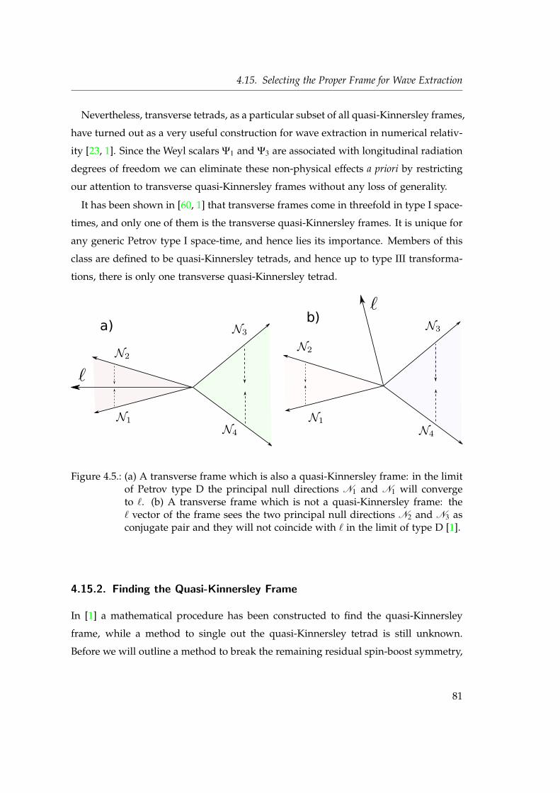
4.15. Selecting the Proper Frame for Wave Extraction
Nevertheless, transverse tetrads, as a particular subset of all quasi-Kinnersley frames,
have turned out as a very useful construction for wave extraction in numerical relativ-
ity [23, 1]. Since the Weyl scalars Ψ1 and Ψ3 are associated with longitudinal radiation
degrees of freedom we can eliminate these non-physical effects a priori by restricting
our attention to transverse quasi-Kinnersley frames without any loss of generality.
It has been shown in [60, 1] that transverse frames come in threefold in type I space-
times, and only one of them is the transverse quasi-Kinnersley frames. It is unique for
any generic Petrov type I space-time, and hence lies its importance. Members of this
class are defined to be quasi-Kinnersley tetrads, and hence up to type III transforma-
tions, there is only one transverse quasi-Kinnersley tetrad.
a)b)
Figure 4.5.: (a) A transverse frame which is also a quasi-Kinnersley frame: in the limitof Petrov type D the principal null directions N1 and N1 will convergeto `. (b) A transverse frame which is not a quasi-Kinnersley frame: the` vector of the frame sees the two principal null directions N2 and N3 asconjugate pair and they will not coincide with ` in the limit of type D [1].
4.15.2. Finding the Quasi-Kinnersley Frame
In [1] a mathematical procedure has been constructed to find the quasi-Kinnersley
frame, while a method to single out the quasi-Kinnersley tetrad is still unknown.
Before we will outline a method to break the remaining residual spin-boost symmetry,
81
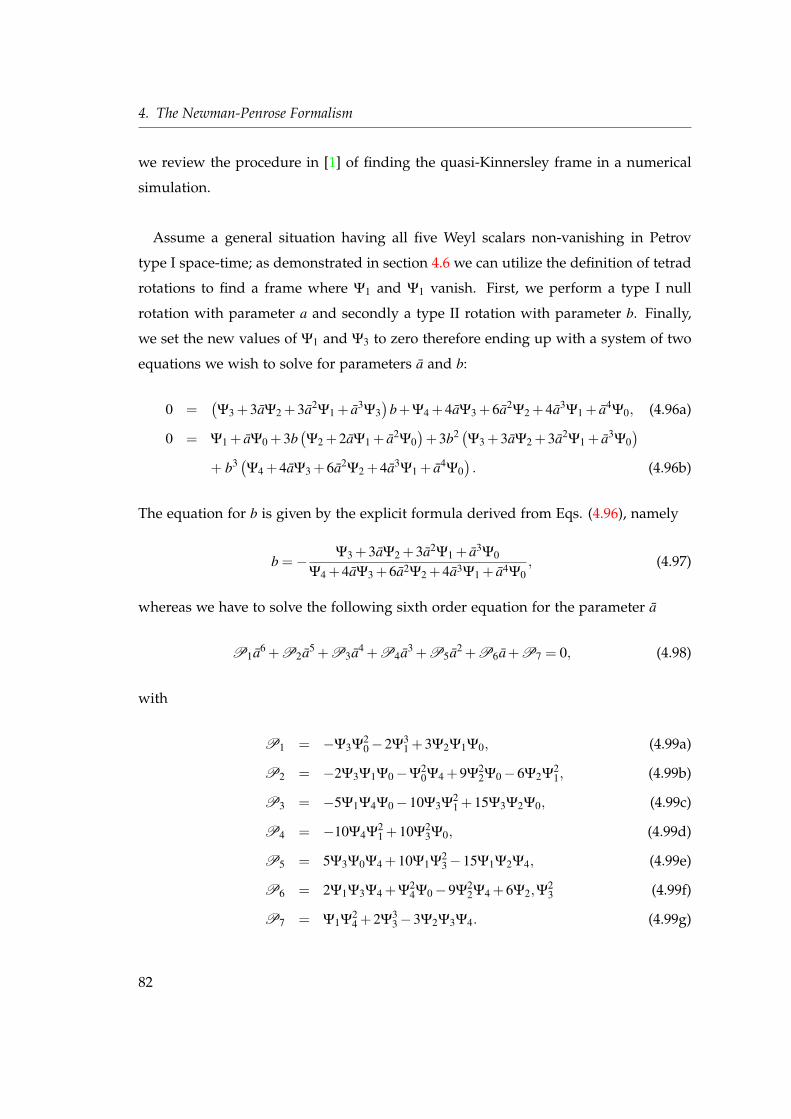
4. The Newman-Penrose Formalism
we review the procedure in [1] of finding the quasi-Kinnersley frame in a numerical
simulation.
Assume a general situation having all five Weyl scalars non-vanishing in Petrov
type I space-time; as demonstrated in section 4.6 we can utilize the definition of tetrad
rotations to find a frame where Ψ1 and Ψ1 vanish. First, we perform a type I null
rotation with parameter a and secondly a type II rotation with parameter b. Finally,
we set the new values of Ψ1 and Ψ3 to zero therefore ending up with a system of two
equations we wish to solve for parameters a and b:
0 =(Ψ3 +3aΨ2 +3a2
Ψ1 + a3Ψ3)
b+Ψ4 +4aΨ3 +6a2Ψ2 +4a3
Ψ1 + a4Ψ0, (4.96a)
0 = Ψ1 + aΨ0 +3b(Ψ2 +2aΨ1 + a2
Ψ0)+3b2 (
Ψ3 +3aΨ2 +3a2Ψ1 + a3
Ψ0)
+ b3 (Ψ4 +4aΨ3 +6a2
Ψ2 +4a3Ψ1 + a4
Ψ0). (4.96b)
The equation for b is given by the explicit formula derived from Eqs. (4.96), namely
b =− Ψ3 +3aΨ2 +3a2Ψ1 + a3Ψ0
Ψ4 +4aΨ3 +6a2Ψ2 +4a3Ψ1 + a4Ψ0, (4.97)
whereas we have to solve the following sixth order equation for the parameter a
P1a6 +P2a5 +P3a4 +P4a3 +P5a2 +P6a+P7 = 0, (4.98)
with
P1 = −Ψ3Ψ20−2Ψ
31 +3Ψ2Ψ1Ψ0, (4.99a)
P2 = −2Ψ3Ψ1Ψ0−Ψ20Ψ4 +9Ψ
22Ψ0−6Ψ2Ψ
21, (4.99b)
P3 = −5Ψ1Ψ4Ψ0−10Ψ3Ψ21 +15Ψ3Ψ2Ψ0, (4.99c)
P4 = −10Ψ4Ψ21 +10Ψ
23Ψ0, (4.99d)
P5 = 5Ψ3Ψ0Ψ4 +10Ψ1Ψ23−15Ψ1Ψ2Ψ4, (4.99e)
P6 = 2Ψ1Ψ3Ψ4 +Ψ24Ψ0−9Ψ
22Ψ4 +6Ψ2,Ψ
23 (4.99f)
P7 = Ψ1Ψ24 +2Ψ
33−3Ψ2Ψ3Ψ4. (4.99g)
82
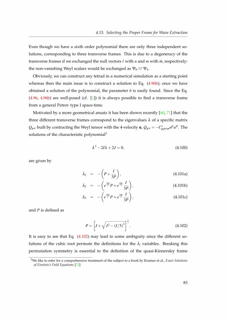
4.15. Selecting the Proper Frame for Wave Extraction
Even though we have a sixth order polynomial there are only three independent so-
lutions, corresponding to three transverse frames. This is due to a degeneracy of the
transverse frames if we exchanged the null vectors ` with n and m with m, respectively:
the non-vanishing Weyl scalars would be exchanged as Ψ0Ψ4.
Obviously, we can construct any tetrad in a numerical simulation as a starting point
whereas then the main issue is to construct a solution to Eq. (4.96b); once we have
obtained a solution of the polynomial, the parameter b is easily found. Since the Eq.
(4.96, 4.96b) are well-posed (cf. [1]) it is always possible to find a transverse frame
from a general Petrov type I space-time.
Motivated by a more geometrical ansatz it has been shown recently [60, 71] that the
three different transverse frames correspond to the eigenvalues λ of a specific matrix
Qµν built by contracting the Weyl tensor with the 4-velocity u, Qµν =−C∗µρνσ uρuσ . The
solutions of the characteristic polynomial3
λ3−2Iλ +2J = 0, (4.100)
are given by
λ1 = −(
P+I
3P
), (4.101a)
λ2 = −(
e2πi3 P+ e
4πi3
I3P
), (4.101b)
λ3 = −(
e4πi3 P+ e
2πi3
I3P
), (4.101c)
and P is defined as
P =[
J +√
J2− (I/3)3] 1
3
. (4.102)
It is easy to see that Eq. (4.102) may lead to some ambiguity since the different so-
lutions of the cubic root permute the definitions for the λi variables. Breaking this
permutation symmetry is essential to the definition of the quasi-Kinnersley frame
3We like to refer for a comprehensive treatment of the subject to a book by Kramer et al., Exact Solutionsof Einstein’s Field Equations [72]
83

4. The Newman-Penrose Formalism
[60]. It can further be shown that the coulomb scalar Ψ2 can be related to the three
eigenvalues λ , namely
ΨI2 =
12
λ1, (4.103a)
ΨII2 =
12
λ2, (4.103b)
ΨIII2 =
12
λ3, (4.103c)
The product of the transverse scalars can be specified accordingly
(Ψ0Ψ4)I =
(λ II−λ III
)2
4, (4.104)
(Ψ0Ψ4)II =
(λ I−λ III
)2
4, (4.105)
(Ψ0Ψ4)III =
(λ I−λ II
)2
4. (4.106)
Thus, we are finally left with two methods to calculate all non-vanishing Weyl scalars
in the three transverse frames. However, we are faced with a residual (type III) ambi-
guity in both approaches; We do not know the exact value of Ψ0 and Ψ4 but only the
product Ψ0Ψ4, respectively.
84

85

86
5. Non-Perturbative Approach for Wave
Extraction
I have noticed even people who claim everything is predestined,
and that we can do nothing to change it, look before they cross the road.
Stephen Hawking
In chapter 4 we presented the fundamental equations and physical results related to
the Newman-Penrose formalism. We have introduced the Weyl scalars and demon-
strated that they, extracted in a particular frame (the Kinnersley tetrad [16]), acquire
a precise physical meaning. In fact, they carry all information about the space-time
under consideration. In particular, we have demonstrated how Ψ4 and Ψ0 can be
identified with the outgoing and ingoing gravitational radiation, respectively.
In section 4.15 we introduced the notion of transverse tetrads, satisfying the condition
Ψ1 = Ψ3 = 0, and explained why those tetrads constitute a particular suitable choice
for wave extraction. Furthermore, we described the most frequently applied method
to find transverse frames in a numerical simulation; that is to calculate the Weyl scalars
using an initial tetrad, and then calculate the rotation parameters for type I and type II
rotations using the two methods given in [60, 1, 23]. This procedure is rather lengthy
to apply in practice; moreover, the condition Ψ1 = Ψ3 = 0 itself does not fix the tetrad
completely1, leaving a spin-boost (type III rotation) ambiguity. As we discussed in
section 4.11, Kinnersley imposed the additional condition ε = 0 to break the remaining
symmetry.
Finally, we outlined a method to find the quasi-Kinnersley frame, as a tetrad frame
defined for a general type I space-time. It turned out that the quasi-Kinnersley frame is1only 4 of the 6 degrees of freedom of the Lorentz group of transformations are fixed
87
5. Non-Perturbative Approach for Wave Extraction
part of a general set of frames which satisfy the property Ψ0Ψ4→ 0 when approaching
the limit of type D (cf. Def. 3). By defining the Weyl scalars in this particular frame
we assure that we recover Teukolsky’s results in the limit of Type D. An equivalent
statement is made by the peeling theorem [73, 18].
5.1. A new Formalism for Wave Extraction
In this chapter we will propose a new approach for wave extraction. We will present
a general method in the Newman-Penrose formalism that relates the Weyl scalars
to the connection coefficients (spin coefficients) when a specific choice of tetrad is
performed, namely the one in which Ψ1 = Ψ3 = 0 and Ψ0 = Ψ4, which always exists in
a general Petrov type I space-time. We use the approach to fix the optimal tetrad for
gravitational wave extraction in numerical relativity, in particular by giving a canonical
expression for the spin-boost parameter that was still unclear. The Weyl scalars Ψ0,
Ψ2 and Ψ4 are given as functions of the two space-time invariants I and J.
In fact, imposing the condition Ψ0 = Ψ4, what corresponds to B = 1 for the spin-boost
degree of freedom, is not the best possible choice, since in this case the two transverse
Weyl scalars have the radial fall-off of r−3 at future null infinity, which is contradictory
to the prediction of the peeling-off theorem (cf. section 4.8). Nevertheless, we can use
this choice as a starting point and reinsert the spin-boost degree of freedom into the
expressions for the scalars.
The chapter is organized as follows: In section 5.2 we deduce a new expression
for the three non-vanishing Weyl scalars Ψ0, Ψ2 and Ψ4 in the transverse frames. In
section 5.3 through section 5.5 we introduce the directional derivatives and analyze the
Bianchi and Ricci identities in the transverse frames; moreover, we study the equations
in the limit of Petrov type D. In section 5.6 we will show that the Bianchi identities
provide a unique relation between spin coefficients in the limit of Petrov type D. An
expression for ε is then obtained using the Ricci identities in section 5.7. Finally in
section 5.8 we enforce the condition ε = 0 and obtain the corresponding spin-boost
parameter. This result leads to the final expression for the Weyl scalars in section 5.9.
88
5.2. Redefining the Weyl Scalars in Transverse Frames
5.2. Redefining the Weyl Scalars in Transverse Frames
By requiring these two conditions, namely Ψ1 = Ψ3 = 0 and Ψ0 = Ψ4, the expressions
for the two curvature invariants introduced in Eqs. (4.36) simplify to
I = Ψ24 +3Ψ
22, (5.1a)
J = Ψ24Ψ2−Ψ
32. (5.1b)
As discussed in detail in chapter 4 we recall that Ψ2 is given by Ψ2 = 12 λi, where λi
represents the three different solutions of the characteristic polynomial
λ3−2Iλ +2J = 0. (5.2)
The three possible solutions are given by
λ1 = −(
P+I
3P
), (5.3a)
λ2 = −(
e2πi3 P+ e
4πi3
I3P
), (5.3b)
λ3 = −(
e4πi3 P+ e
2πi3
I3P
), (5.3c)
where P is defined as
P =[
J +√
J2− (I/3)3] 1
3
. (5.4)
Eq. (5.1a) and Eq. (5.1b) can now be inverted to give not only Ψ2 but also Ψ4 as
a function of the curvature invariants I and J. We start redefining the scalars by
introducing the important variable Ψ±, which unifies the three different solutions for
the scalars in Eq. (5.3),
Ψ± = I12
(e
2πik3 Θ± e−
2πik3 Θ
−1)
, (5.5)
where k is an integer number assuming the values 0,1,2 corresponding to the three
different transverse frames and Θ is defined according to
89
5. Non-Perturbative Approach for Wave Extraction
Θ =√
3PI−12 . (5.6)
It is worth noting that a key ingredient for establishing our new methodology is rewrit-
ing the Bianchi identities in terms of these newly introduced variables Ψ±. We can
now rewrite the three non-vanishing scalars in the transverse frames in the following
manner
Ψ0 = − iB−2
2·Ψ−, (5.7a)
Ψ2 = − 12√
3·Ψ+, (5.7b)
Ψ4 = − iB2
2·Ψ−, (5.7c)
where we have reinserted the spin-boost parameter B,
B =(
Ψ4
Ψ0
) 14
. (5.8)
We want to stress the behavior of the introduced quantities in the limit of type D
(cf. section 4.15). The speciality index in Eq. (4.37) reduces to S→ 1 from what we
immediately deduce the behavior of the space-time invariants in the type D limit
J →√
I3/27, (5.9a)
P → I1/2/√
3, (5.9b)
and thus the quantity Θ in Eq. (5.6) reduces to
Θ→ 1. (5.10)
We now evaluate the quantities Ψ± in Eq. (5.5) for the frame with k = 0, yielding
Ψ+ = I12(Θ+Θ
−1)→ 2I12 , (5.11a)
Ψ− = I12(Θ−Θ
−1)→ 0, (5.11b)
90
5.3. The Bianchi Identities
and consequently, the original Weyl scalars simplify in Petrov type D according to
Ψ0 = − iB−2
2·Ψ−→ 0, (5.12a)
Ψ2 = − 12√
3·Ψ+→−I1/2/
√3, (5.12b)
Ψ4 = − iB2
2·Ψ−→ 0. (5.12c)
Since Ψ0 and Ψ4 tend to zero in Petrov type D we can conclude, by utilizing Def.
3, that the frame with k = 0 is the transverse frame which is also a quasi-Kinnersley
frame.
5.3. The Bianchi Identities
In chapter 4 we introduced the Bianchi identities and defined the projection on to
a tetrad frame. We now deduce the explicit expressions of all non-trivial terms in
the Newman-Penrose formalism, given here in terms of the Weyl scalars and spin
coefficients. As mentioned in section 4.1 the Bianchi identities can be expressed in the
Newman-Penrose formalism according to
R(a)(b)[(c)(d)|( f )] =16 ∑
[(c)(d)( f )]
R(a)(b)(c)(d),( f )
−η(n)(m)
[γ(n)(a)( f )R(m)(b)(c)(d) + γ(n)(b)( f )R(a)(m)(c)(d)
+γ(n)(c)( f )R(a)(b)(m)(d) + γ(n)(d)( f )R(a)(b)(c)(m)
]. (5.13)
Written out explicitly, all non-vanishing identities in a vacuum space-time are given
by the eight following complex identities
−δ∗Ψ0 +DΨ1−2(2ρ + ε)Ψ1 +3κΨ2 +(4α−π)Ψ0 = 0, (5.14a)
−δ∗Ψ2 +DΨ3 +κΨ4−3πΨ2 +2λΨ1 +2(ε−ρ)Ψ3 = 0, (5.14b)
−DΨ2 +δ∗−λΨ0 +3ρΨ2 +2(π−α)Ψ1−2κΨ3 = 0, (5.14c)
−δ∗Ψ3 +DΨ4 +3λΨ2−2(2π +α)Ψ3 +(4ε−ρ)Ψ4 = 0, (5.14d)
91
5. Non-Perturbative Approach for Wave Extraction
−∆Ψ0 +3σΨ2 +(4γ−µ)Ψ0δΨ1−2(2τ +β )Ψ1 = 0, (5.14e)
−∆Ψ1 +δΨ2 +νΨ0 +2(γ−µ)Ψ1−3τΨ2 +2σΨ3 = 0, (5.14f)
−∆Ψ2 +δΨ3 +2νΨ1 +σΨ4 +2(β − τ)Ψ3−3µΨ2 = 0, (5.14g)
−∆Ψ3 +δΨ4 +3νΨ2−2(γ +2µ)Ψ3− (τ−4β )Ψ4 = 0. (5.14h)
There seems to be no obvious structure in the equations. But since we want to focus
our attention on the expressions of the scalars in the transverse frames, we enforce the
condition Ψ1 = Ψ3 = 0, considerably simplifying the Bianchi identities:
DΨ4 = −3λΨ2− (4ε−ρ)Ψ4, (5.15a)
DΨ2 = −λΨ0 +3ρΨ2, (5.15b)
∆Ψ0 = 3σΨ2 +(4γ−µ)Ψ0, (5.15c)
∆Ψ2 = σΨ4−3µΨ2, (5.15d)
δΨ4 = −3νΨ2 +(τ−4β )Ψ4, (5.15e)
δΨ2 = −νΨ0 +3τΨ2, (5.15f)
δ∗Ψ0 = 3κΨ2 +(4α−π)Ψ0, (5.15g)
δ∗Ψ2 = κΨ4−3πΨ2. (5.15h)
We want to stress that we have recast the equations in a more convenient form to
highlight the now appearing structure; we get a set of two coupled equations for
every directional derivative.
5.4. The Ricci Identities
We will perform a similar procedure with the Ricci identities as done with the Bianchi
identities. According to section 4.1 the Ricci identities are defined in the tetrad for-
malism as
R(a)(b)(c)(d) = − γ(a)(b)(c),(d) + γ(a)(b)(d),(c)− γ(b)(a)( f )
[γ
( f )(c) (d)− γ
( f )(d) (c)
]+ γ( f )(a)(c)γ
( f )(b) (d)− γ( f )(a)(d)γ
( f )(b) (c). (5.16)
92
5.4. The Ricci Identities
By projecting all non-vanishing Ricci identities on to the Newman-Penrose tetrad we
yield a set of 18 complex equations:
Dρ−δ∗κ =
(ρ
2 +σσ∗)+ρ (ε + ε
∗)−κ∗τ−κ (3α +β
∗−π) , (5.17a)
Dσ −δκ = σ (ρ +ρ∗+3ε− ε
∗)−κ (τ−π∗+α
∗+3β )+Ψ0, (5.17b)
Dτ−∆κ = ρ (τ +π∗)+σ (τ∗+π)+ τ (ε− ε
∗)−κ (3γ + γ∗)+Ψ1, (5.17c)
Dα−δ∗ε = α (ρ + ε
∗−2ε)+π (ε +ρ)+βσ∗−β
∗ε−κλ −κ
∗γ, (5.17d)
Dβ −δε = σ (α +π)+β (ρ∗− ε∗)−κ (µ + γ)− ε (α∗−π
∗)+Ψ1, (5.17e)
Dγ−∆ε = α (τ +π∗)+β (τ∗+π)+ τπ− γ (ε + ε
∗)− ε (γ + γ∗)−νκ +Ψ2, (5.17f)
Dλ −δ∗π = ρλ +σ
∗µ +π (π +α−β
∗)−λ (3ε− ε∗)−νκ
∗, (5.17g)
Dµ−δπ = ρ∗µ +σλ +π (π +α−β
∗)−λ (3ε− ε∗)−νκ +Ψ2, (5.17h)
δρ−δ∗σ = ρ (α∗+β )−σ (3α−β
∗)+ τ (ρ−ρ∗)+κ (µ−µ
∗)−Ψ1. (5.17i)
The other nine Ricci identities can be obtained by swapping the tetrad vectors ` with
n and m with m.
In contrast to the Bianchi identities the Ricci identities do not simplify noticeable by
enforcing the condition Ψ1 = Ψ3 = 0,
Dρ−δ∗κ =
(ρ
2 +σσ∗)+ρ (ε + ε
∗)−κ∗τ−κ (3α +β
∗−π) , (5.18a)
Dσ −δκ = σ (ρ +ρ∗+3ε− ε
∗)−κ (τ−π∗+α
∗+3β )+Ψ0, (5.18b)
Dτ−∆κ = ρ (τ +π∗)+σ (τ∗+π)+ τ (ε− ε
∗)−κ (3γ + γ∗) , (5.18c)
Dα−δ∗ε = α (ρ + ε
∗−2ε)+π (ε +ρ)+βσ∗−β
∗ε−κλ −κ
∗γ, (5.18d)
Dβ −δε = σ (α +π)+β (ρ∗− ε∗)−κ (µ + γ)− ε (α∗−π
∗) , (5.18e)
Dγ−∆ε = α (τ +π∗)+β (τ∗+π)+ τπ− γ (ε + ε
∗)− ε (γ + γ∗)−νκ +Ψ2, (5.18f)
Dλ −δ∗π = ρλ +σ
∗µ +π (π +α−β
∗)−λ (3ε− ε∗)−νκ
∗, (5.18g)
Dµ−δπ = ρ∗µ +σλ +π (π +α−β
∗)−λ (3ε− ε∗)−νκ +Ψ2, (5.18h)
δρ−δ∗σ = ρ (α∗+β )−σ (3α−β
∗)+ τ (ρ−ρ∗)+κ (µ−µ
∗) . (5.18i)
93
5. Non-Perturbative Approach for Wave Extraction
5.5. Directional Derivatives
From the definition of the Lie bracket we derive a set of relations for the commutators
and for the double derivatives in the Newman-Penrose formalism. As an example we
calculate the Lie bracket of [∆,D]:
[∆,D] = [n, `] =−γ121∆+ γ212D− (γ312− γ321)δ∗− (γ412− γ421)δ . (5.19)
Introducing the designated symbols of the spin coefficients we derive the full set of
commutation relations
[∆,D] = (γ + γ∗)D+(ε + ε
∗)∆− (τ∗+π)δ − (τ +π∗)δ
∗, (5.20a)
[δ ,D] = (α +β −π∗)D+κ∆− (ρ∗+ ε− ε
∗)δ − (τ +π∗)δ
∗, (5.20b)
[δ ,∆] = −ν∗D+(τ−α
∗−β )∆+(µ− γ + γ∗)δ +λ
∗δ∗, (5.20c)
[δ ,δ ∗] = (µ∗−µ)D+(ρ∗−ρ)∆+(α−β
∗)δ +(β −α∗)δ
∗, (5.20d)
[δ ∗,∆] = −νD+(τ∗−α−β∗)∆+(µ
∗− γ∗+ γ)δ
∗+λδ , (5.20e)
[δ ∗,D] = (α∗+β∗−π)D+κ
∗∆− (ρ + ε
∗− ε)δ∗− (τ∗+π)δ . (5.20f)
Furthermore, we can calculate double derivatives in the Newman-Penrose formal-
ism:
DD = (ε + ε∗)D−κ
∗δ −κδ
∗+ `µ`ν∇µ∇ν , (5.21a)
∆∆ = −(γ + γ∗)∆+νδ +ν
∗δ∗+nµnν
∇µ∇ν , (5.21b)
δδ = λ∗D−σ∆+(β −α
∗)δ +mµmν∇µ∇ν , (5.21c)
δ∗δ∗ = λD−σ
∗∆− (α−β
∗)δ∗+ mµmν
∇µ∇ν , (5.21d)
∆D = (γ + γ∗)D− τ
∗δ − τδ
∗+nµ`ν∇µ∇ν , (5.21e)
D∆ = −(ε + ε∗)∆+πδ +π
∗δ∗+ `µnν
∇µ∇ν , (5.21f)
Dδ = π∗D−κ∆+(ε− ε
∗)δ + `µmν∇µ∇ν , (5.21g)
δD = (β +α∗)D−ρ
∗δ −σδ
∗+mµ`ν∇µ∇ν , (5.21h)
94
5.5. Directional Derivatives
Dδ∗ = πD−κ
∗∆− (ε− ε
∗)δ∗+ `µmν
∇µ∇ν , (5.21i)
δ∗D = (β ∗+α)D−σ
∗δ −ρδ
∗+ mµ`ν∇µ∇ν , (5.21j)
∆δ = ν∗D− τ∆+(γ− γ
∗)δ +nµmν∇µ∇ν , (5.21k)
δ∆ = −(β +α∗)∆+ µδ +λ
∗δ∗+mµnν
∇µ∇ν , (5.21l)
∆δ∗ = νD− τ
∗∆− (γ− γ
∗)δ∗+nµmν
∇µ∇ν , (5.21m)
δ∗∆ = −(β ∗+α)∆+λδ + µ
∗δ∗+ mµnν
∇µ∇ν , (5.21n)
δδ∗ = µD−ρ
∗∆− (β −α
∗)δ∗+mµmν
∇µ∇ν , (5.21o)
δ∗δ = µ
∗D−ρ∆+(α−β∗)δ + mµmν
∇µ∇ν . (5.21p)
We will make use of these directional derivatives and double derivatives in section 5.8
to determine the function H.
95
5. Non-Perturbative Approach for Wave Extraction
5.6. The Type D Spin Relation
As already mentioned, a key ingredient for the derivation of our new extraction for-
malism is rewriting the Bianchi identities in Eqs. (5.15, 5.18) in terms of the newly in-
troduced variables Ψ±. Since ε appears only in the first two Bianchi identities, namely
Eqs. (5.15a, 5.15b), we will give the details of the calculation only for the derivative
operator D; however, as the symmetry of the Bianchi identities suggests, the calcula-
tion for the other derivatives is analogous and trivial to perform, and we will use the
symmetry properties at the end of this chapter to deduce the expressions for the spin
coefficients γ , α and β .
We start by inserting Eq. (5.7), which relate the Weyl scalars Ψ0, Ψ2 and Ψ4 to the
new scalars Ψ+ and Ψ−, into the Bianchi identities yielding
DΨ+ = −λΨ−+3ρΨ+, (5.22a)
DΨ− = λΨ+− (4ε−ρ)Ψ−, (5.22b)
∆Ψ+ = σΨ−−3µΨ+, (5.22c)
∆Ψ− = −σΨ+ +(4γ−µ)Ψ−, (5.22d)
δΨ+ = −νΨ−+3τΨ+, (5.22e)
δΨ− = νΨ+−(
4β − τ
)Ψ−, (5.22f)
δ∗Ψ+ = κΨ−−3πΨ+, (5.22g)
δ∗Ψ− = −κΨ+ +(4α−π)Ψ−, (5.22h)
where we have additionally introduced the rescaled spin coefficients
λ = i√
3λB−2, (5.23a)
σ = i√
3σB2 (5.23b)
ν = i√
3νB−2, (5.23c)
κ = i√
3κB2, (5.23d)
96
5.6. The Type D Spin Relation
and
ε = ε +12
D lnB, (5.23e)
γ = γ +12
∆ lnB, (5.23f)
β = β +12
δ lnB, (5.23g)
α = α +12
δ∗ lnB. (5.23h)
This new set of rescaled spin coefficients now transforms in the same way under a
spin-boost transformation (cf. section 4.6): for example the three spin coefficientsρ, λ , ε
transform according to
ρ → |B|−1ρ, (5.24a)
ε → |B|−1ε, (5.24b)
λ → |B|−1λ , (5.24c)
and analogous transformations for the other spin coefficients.
These transformation properties are not a surprising result when we consider how
the individual quantities in Eq. (5.22a) and Eq. (5.22b) transform under a type III
rotation:
Ψ+ and Ψ− are only functions of curvature invariants, therefore the only dependence
on the spin-boost parameter on the left hand side comes from the `µ null vector of
the D derivative operator which carries a |B|−1 factor. Obviously, the right hand side
must be consistent and show the same spin-boost dependence in the rescaled spin
coefficients, what is in fact the case as demonstrated in Eqs. (5.24).
We will now study the behavior of the Bianchi identities in the Petrov type D limit.
By dividing Eq. (5.22a) by Ψ+ and Eq. (5.22b) by Ψ− the first two Bianchi identities
97
5. Non-Perturbative Approach for Wave Extraction
become:
DΨ+
Ψ+= −λ
Ψ−Ψ+
+3ρ, (5.25a)
DΨ−Ψ−
= λΨ+
Ψ−− (4ε−ρ) . (5.25b)
Employing the definition of Ψ± in Eq. (5.5) and applying the D operator to Ψ+ and
Ψ− gives
DΨ+ = D lnΘ ·Ψ−+D ln(
I12
)Ψ+, (5.26a)
DΨ− = D lnΘ ·Ψ+ +D ln(
I12
)Ψ−. (5.26b)
In the limit of Petrov type D, what corresponds to Θ → 1 as demonstrated, these
equations simplify to:
DΨ+→ D ln(
I12
)Ψ+, (5.27a)
DΨ−→ D ln(
I12
)Ψ−. (5.27b)
This result implies that the left hand sides in Eq. (5.25) tend to the same value in type
D, namely D ln(
I12
), and therefore also the right hand sides can be set to be equal in
this limit. Moreover, from the definition of Ψ± we can calculate the limit of the ratioΨ−Ψ+
, in fact
Ψ−Ψ+
=I
12
(e
2πik3 Θ− e−
2πik3 Θ−1
)I
12
(e
2πik3 Θ+ e−
2πik3 Θ−1
) →(
e2πik
3 − e−2πik
3
)(
e2πik
3 + e−2πik
3
) =−i tan(
2πk3
). (5.28)
Putting this all together, and subtracting Eq. (5.25b) from Eq. (5.25a) we find that the
following relation between spin coefficients holds in the Petrov type D limit
(ρ +2ε)sin(
4πk3
)+ iλ cos
(4πk
3
)= 0, (5.29)
which we call the type D spin relation. Eq. (5.29) is valid for all three transverse frames,
98
5.7. Spin Coefficients as Directional Derivatives
depending on the value of k.
If we assume to be in the transverse frame that is also a quasi-Kinnersley frame, which
corresponds to having k = 0, Eq. (5.29) reduces to λ = 0 consistently with the Goldberg-
Sachs theorem (cf. section 4.9). Nevertheless, by combining Eq. (5.22a) and Eq. (5.27a)
we can deduce the expression for one of the spin coefficients, namely ρ , in terms of
curvature invariants
ρ = D ln I16 . (5.30)
But the key point to stress here is that in the quasi-Kinnersley frame the Bianchi
identities leave the expression for ε completely unresolved. However, it is really the
expression for ε we are interested in, as it is the one related to the spin-boost transfor-
mation. To obtain additional information on this spin coefficient, we therefore analyze
the Ricci identities.
5.7. Spin Coefficients as Directional Derivatives
In this section, we will use the Ricci identities to understand how the spin coefficients
ε , γ , α and β relate to the spin-boost parameter B. We will first show that they can
be expressed as directional derivatives of the same function, and then determine the
equation that this function must satisfy in the limit of Petrov type D.
We start by assuming to be in the Petrov type D limit, where Ψ0 = Ψ1 = Ψ3 = Ψ4 = 0
and also, as a consequence of the Goldberg-Sachs theorem, the four spin coefficients
λ , σ , ν and κ are vanishing (cf. section 4.9). We begin with the following Ricci identity
(5.18e),
Dβ −δε = σ (α +π)+β (ρ∗− ε∗)−κ (µ + γ)− ε (α∗−π
∗) , (5.31)
simplifying in the limit of type D to
Dβ −δε = β (ρ∗− ε∗)− ε (α∗−π
∗) . (5.32)
Here we obtain, after adding and subtracting the product βε on the right-hand side,
99
5. Non-Perturbative Approach for Wave Extraction
the relation:
Dβ −δε = ε (π∗−α∗−β )+β (ρ∗+ ε− ε
∗) . (5.33)
By inserting the definition of the rescaled spin coefficients ε and β in Eq. (5.23) we
can re-express this Ricci identity in terms of ε and β , leading to
Dβ −δ ε = ε (π∗−α∗−β )+ β (ρ∗+ ε− ε
∗) . (5.34)
Comparing Eq. (5.34) with the expression of the commutator [D,δ ] (again assuming
σ = κ = 0) in Eq. (5.20b), namely
[D,δ ] = Dδ −δD = (π∗−α∗−β )D+(ρ∗+ ε− ε
∗)δ , (5.35)
it is possible to see that these equations are consistent by assuming ε = DH1 and
β = δH1, where H1 is a function to be determined. Using the equivalent Ricci identity
obtained after exchanging the tetrad vectors `↔ n and m↔ m,
∆α−δ∗γ = α (γ∗− γ−µ
∗)+ γ (α +β∗− τ
∗) , (5.36)
we obtain an equivalent result for the spin coefficients γ and α when compared to
the commutator [∆,δ ∗] in Eq. (5.20e) and conclude that they also can be expressed as
γ = ∆H2 and α = δ ∗H2, where H2 is a function to be determined.
Using the properties of transformation of the spin coefficients under the exchange
operation `µ ↔ nµ and mµ ↔ mµ , which corresponds to exchanging ε ↔−γ and α ↔
−β , we can immediately conclude that
H1 =−H2 = H , (5.37)
where H is still to be determined. Nevertheless, the four spin coefficients can then be
written as
ε = DH , γ =−∆H , (5.38a)
β = δH , α =−δ∗H , (5.38b)
100
5.8. The Function H
and the original spin coefficients are therefore given by
ε = DH − 12
D lnB = DH−, (5.39a)
γ = −∆H − 12
∆ lnB =−∆H+, (5.39b)
β = δH − 12
δ lnB = δH−, (5.39c)
α = −δ∗H − 1
2δ∗ lnB =−δ
∗H+, (5.39d)
where we have introduced the additional quantity H± = H ± 12 lnB.
In the next section we make use of some other Ricci identities to find the explicit
expression for H .
5.8. The Function H
To determine the function H we consider the two following Ricci identities
Dγ−∆ε = α (τ +π∗)+β (τ∗+π)+ τπ− γ (ε + ε
∗)− ε (γ + γ∗)+Ψ2, (5.40a)
δα−δ∗β = µρ +αα
∗+ββ∗−2αβ + γ (ρ−ρ
∗)+ ε (µ−µ∗)−Ψ2. (5.40b)
Again, by utilizing the rescaled spin coefficients in Eq. (5.23) we can remove the
spin-boost dependence in these identities, yielding
Dγ−∆ε = α (τ +π∗)+ β (τ∗+π)+ τπ− γ (ε + ε
∗)− ε (γ + γ∗)+Ψ2, (5.41a)
δ α−δ∗β = µρ + αα
∗+ ββ∗−2αβ + γ (ρ−ρ
∗)+ ε (µ−µ∗)−Ψ2. (5.41b)
Since we have just found that the reduced spin coefficients on the left-hand sides can
be expressed as directional derivatives of H , cf. Eq. (5.38), we yield terms of the form
D∆H or δδH among others.
Thus, we can use the definition of double derivatives in Eq. (5.21) to find an equiv-
alent form of Eq. (5.40) or Eq. (5.41), respectively. The particular equations we will
101
5. Non-Perturbative Approach for Wave Extraction
make use of are the following
D∆ = −(ε + ε∗)∆+πδ +π
∗δ∗+ `µnν
∇µ∇ν , (5.42a)
∆D = (γ + γ∗)D− τ
∗δ − τδ
∗+nµ`ν∇µ∇ν , (5.42b)
δδ∗ = µD−ρ
∗∆− (β −α
∗)δ∗+mµmν
∇µ∇ν , (5.42c)
δ∗δ = µ
∗D−ρ∆+(α−β∗)δ + mµmν
∇µ∇ν . (5.42d)
As an example, we calculate the term Dγ on the left hand side of Eq. (5.41a). Using
the property just found that in the Petrov type D limit γ =−∆H , this term is given by
Dγ =−D∆H , (5.43)
and using Eq. (5.42a) this corresponds to
Dγ =−D∆H = (ε + ε∗)∆H −πδH −π
∗δ∗H − `µnν
∇µ∇νH . (5.44)
If we substitute α =−δ ∗H and β = δH we yield
Dγ = −(ε + ε∗) γ−πβ +π
∗α− `µnν
∇µ∇νH . (5.45)
By repeating the same procedure for ∆ε , δ α and δ ∗β and comparing the expressions
with the Ricci identities in Eq. (5.41) we finally end up with the following two identities
for the function H :
2`µnν∇µ∇νH = −2πβ −2τα−πτ−Ψ2, (5.46a)
2mµmν∇µ∇νH = −2µε−2ργ−µρ +Ψ2. (5.46b)
As a last step, we subtract Eq. (5.46b) from Eq. (5.46a) and utilize the definition of the
metric in the tetrad, namely
gµν = 2`(µnν)−2m(µmν), (5.47)
102
5.9. Weyl Scalars in Terms of Curvature Invariants
thus obtaining the master equation for H :
∇µ
∇µH +∇µ ln(
I16
)∇µ
(2H + ln I
112
)=−2Ψ2, (5.48)
where we have also used the fact that in the Petrov type D limit ρ = D ln I16 , µ =−∆ ln I
16 ,
τ = δ ln I16 and π =−δ ∗ ln I
16 .
In the next section we will solve Eq. (5.48) for the single black hole case to obtain
the condition on the spin-boost parameter.
5.9. Weyl Scalars in Terms of Curvature Invariants
We can now apply the results we just found to the particular case of the Kerr solution
using Boyer-Lindquist coordinates. The metric in this case reads (cf. section 4.11, 4.12)
ds2 =(
1− 2MrΣ
)dt2 +
(4Mar sin2
θ
Σ
)dtdφ −
(Σ
Γ
)dr2− Σdθ
2− sin2θ
(∆
Σ
)dφ
2, (5.49)
where Γ = r2−2Mr +a2, Σ = r2 +a2 cos2 θ , ∆ = r2 +a2 +2Mar sin2θ , M is the black hole
mass and a its rotation parameter. The Kinnersley tetrad in this coordinate system is
given by
`µ =1Γ
[(r2 +a2) ,Γ,0,a
], (5.50a)
nµ =1
2Σ
[r2 +a2,−Γ,0,a
], (5.50b)
mµ =1√2ρ
[iasinθ ,0,1, isecθ ] , (5.50c)
where ρ = r + iacosθ .
The solution for Eq. (5.48) in this particular coordinate system can be straightfor-
wardly carried out and reads
H =12
ln(
Γ12 I
16 sinθ
). (5.51)
We now have all the elements to find the values of the spin coefficients ε , γ , β and α
103
5. Non-Perturbative Approach for Wave Extraction
in the limit of type D, and in particular the condition on the spin-boost parameter. As
already shown, the four spin coefficients ε , γ , α and β can be written as follows
ε = DH − 12
D lnB, (5.52a)
γ = −∆H − 12
∆ lnB, (5.52b)
β = δH − 12
δ lnB, (5.52c)
α = −δ∗H − 1
2δ∗ lnB. (5.52d)
This result can be compared with the expressions for the same spin coefficients in the
Kinnersley tetrad, given by
ε = 0, (5.53a)
γ = µ +ρρ∗ (r−M)/2, (5.53b)
β = cotθ/(2√
2ρ), (5.53c)
α = π−β∗. (5.53d)
Let us consider first the spin coefficient ε . Using Eq. (5.52a) and the solution for H
found in Eq. (5.51) we can rewrite ε in the following way
ε =12
D ln(
Γ12 I
16 B−1 sinθ
). (5.54)
In order for this expression to be zero, the function inside the logarithm must be con-
stant with respect to the derivative operator D. Given the form of the Kinnersley tetrad
in Eq. (5.50), one concludes that the D operator corresponds to the simple ∂r deriva-
tive (assuming that the functions do not have a t or φ dependence, which is indeed
the case, as the Kerr space-time is stationary and axisymmetric). As a consequence of
this, ε vanishes if the function on the right hand side is a generic function only of the
coordinate θ . This leads to the following condition on the spin-boost parameter
B = B0 f (θ) I16 Γ
12 sinθ , (5.55)
104
5.9. Weyl Scalars in Terms of Curvature Invariants
where B0 is an integration constant. By rewriting the other spin coefficients in a
similar manner, namely
γ = −12
∆ ln(
Γ12 I
16 B sinθ
), (5.56)
β = −12
δ∗ ln(
Γ12 I
16 B sinθ
), (5.57)
α =12
δ ln(
Γ12 I
16 B−1 sinθ
), (5.58)
we can determine the function f (θ). In fact, it can be easily shown that the spin
coefficient γ given in Eq. (5.53b) is consistent with Eq. (5.55), imposing no further
condition on f (θ).
The spin coefficient β can instead be used to find the unknown function f (θ): the
derivative operator δ is given by
δ = mµ∇µ =
1√2ρ
∂θ , (5.59)
and is therefore related to the θ -dependence of the spin-boost parameter. A straight-
forward calculation yields f (θ) = sin−1θ , consistent also with the spin coefficient α .
Thus, the final result for B reads
B = B0I16 Γ
12 . (5.60)
5.9.1. Final Expressions for the Weyl Scalars and Peeling Behavior
Finally, we want to apply these results to the Weyl scalars; by inserting the expression
of the spin-boost parameter in Eq. (5.60) into the definition of the scalars in Eq. (5.7)
we yield
Ψ0 = − i2B−2
0 ·Γ−1I
16(Θ−Θ
−1) , (5.61a)
Ψ2 = − 12√
3· I
12(Θ+Θ
−1) , (5.61b)
Ψ4 = − i2B2
0 ·ΓI56(Θ−Θ
−1) . (5.61c)
105
5. Non-Perturbative Approach for Wave Extraction
It is remarkable how these expressions for the scalars immediately give the correct
radial fall-offs at future null infinity once the peeling behavior of the Weyl tensor is
assumed:
• The function Γ is only defined in the limit of Petrov type D and gives no radial
contribution at future null infinity.
• Given under the peeling assumption that I ∝ r−6, we find the same result for Θ
as it is the ratio of quantities that have the same radial behavior at future null
infinity, namely
Θ =√
3PI−12 ∝
r−3
r−3 . (5.62)
• In conclusion, the quantities that give a contribution at future null infinity are
the factors I16 , I
12 and I
56 , corresponding to
Ψ0 ∝ r−1, Ψ2 ∝ r−3 and Ψ4 ∝ r−5. (5.63)
The fact that we obtain radial fall-offs for Ψ0 and Ψ4 that are exchanged with respect
to the normal assumption of outgoing radiation in the literature, where Ψ0 ∝ r−5 and
Ψ4 ∝ r−1, is not surprising: this is due to the fact that in the Kinnersley tetrad the null
vector `µ is ingoing while nµ is outgoing. The standard notation requires instead the
opposite situation where `µ is outgoing and nµ is ingoing.
This means that one needs to exchange `µ ↔ nµ to have the right convention, what
in fact results in B→B−1 and the Weyl scalars are changed to
Ψ0 = − i2B2
0 ·ΓI56(Θ−Θ
−1) , (5.64a)
Ψ2 = − 12√
3· I
12(Θ+Θ
−1) , (5.64b)
Ψ4 = − i2B−2
0 ·Γ−1I
16(Θ−Θ
−1) . (5.64c)
giving this time, as expected, the correct radial fall-offs for Ψ0 and Ψ4.
106
5.9. Weyl Scalars in Terms of Curvature Invariants
5.9.2. Conclusion
Eqs. (5.64) are the main result that we propose for wave extraction in numerical rel-
ativity. As evident from the equations, the conditions on the spin coefficients do not
completely fix the values of the Weyl scalars, leaving the constant B0 undetermined.
This is not surprising as such conditions involve the directional derivatives along the
tetrad null vectors and are therefore independent of additional constant multiplication
factors. The optimal value of this integration constant will have to be determined
enforcing the values of the spin coefficients ρ , µ , τ and π . We will present a possible
value for the integration constant in the following chapter 6.
We are also investigating the comparison of these expressions with the analogous
quantities defined in the characteristic formulation of Einstein’s equations [74, 75, 76].
As we expect, this should give us more insights on how to choose this integration
constant from a more theoretical point of view. This is the subject of future work on
this topic.
107

108
6. Distorted Black Hole Space-Times in
the Newman-Penrose Formalism
I was born not knowing and have only had a little time to change that here and there.
Richard Feynman
In this chapter we study on an analytical level how the expressions for the Weyl scalars
depend on the tetrad we choose in a space-time containing distorted black holes. We
will calculate all relevant quantities in the transverse frames, and show how we can
deduce the spin-boost parameter to find the quasi-Kinnersley tetrad. Finally and most
importantly, we will extract the gravitational wave signal and we will demonstrate
the advantage of our approach proposed in chapter 5 compared to commonly used
methods in numerical relativity.
In spirit this work follows [77, 78, 79, 80, 81, 82, 83, 84, 85] in constructing a distorted
black hole by superposing a Schwarzschild space-time and a pure Brill wave space-
time.
In this chapter we will refer to a symmetric tetrad as a transverse tetrad (Ψ1 = Ψ3 = 0)
obeying the additional symmetry Ψ0 = Ψ4. It further satisfies Def. 3, namely Ψ0 =
Ψ4 → 0 for S→ 1, therefore being a member of the quasi-Kinnersley frame. The quasi-
Kinnersley tetrad, belonging to the same frame, obeys the additional condition of ε→ 0
in the limit of type D, thus being equivalent to the Kinnersley tetrad in Petrov type
D. If it is at all necessary to impose the condition ε = 0 in Petrov type I has not been
clarified as to yet. This is partly due to the fact that the Kinnersley tetrad is defined
in Petrov type D, thus a more general definition of that particular tetrad just does not
exist up to date. In this chapter we demonstrate an approach of how to impose this
109
6. Distorted Black Hole Space-Times in the NP Formalism
condition ε = 0 in Petrov type I in general, for the perturbed black hole space-time
under consideration.
6.1. Brill Wave Initial Data
Brill waves have been used by the numerical relativity community from its earliest
days since discovery by Brill. In his original work Brill gave the first positivity of
energy result in General Relativity [77]. Brill waves are an excellent exploration tool
for such purposes because the space-time contains only radiation, it is only radiation.
Moreover, they have been interesting in their own right because they are a particularly
simple solution to the vacuum equations of General Relativity, but rich in structure.
Radiation and evolution of numerically constructed initial data of pure gravitational
waves have already been studied (e.g. [80]) . Brill wave solutions have also shed light
on the problem of accurately defining the mass of numerically generated initial data
sets. They have been used as a test of the Cosmic Censorship (e.g. [26], [86]), moreover
black hole interaction with gravitational waves (e.g. [85]) and gravitational collapse of
Brill waves (e.g. [87]) have been investigated.
6.1.1. Pure Gravitational Waves
Brill originally considered axisymmetric, time symmetric, vacuum initial data for
the Einstein equations of an asymptotically flat hypersurface with R3 topology as a
Cauchy problem, i.e. the initial data consists of a three metric γ i j and the extrin-
sic curvature Ki j. These are vacuum solutions and they satisfy the Hamiltonian and
Momentum constraints which reduce in a vacuum space-time to:
R+K2−Ki jKi j = 0, (6.1)
∇iKij−∇ jKi
i = 0. (6.2)
Here R is the scalar curvature and ∇ the covariant derivatives associated with γ i j. By
enforcing the condition of time symmetry of the initial slice the extrinsic curvature
tensor Ki j vanishes and leaves only the condition R = 0 for the Hamiltonian constraint
110
6.1. Brill Wave Initial Data
to be satisfied. Following York’s Thin-Sandwich decomposition [88] the three metric
can be written in conformal form
γi j = ψ4γi j, (6.3)
where ψ is the conformal factor. The axially symmetric orthogonal three-metric under
consideration takes in polar-like coordinate the form
ds2 = γi j dxi dx j = eq (dρ2 + dz2)+ρ
2 dθ2, (6.4)
where r2 = ρ2 + z2 and q is an (almost arbitrary) function of ρ and z. Brill imposed an
equatorial symmetry condition across the z = 0 plane, that q decays fairly rapidly at
infinity (faster than 1/r) and that it is regular at ρ = 0:
∂q∂ z|z=0 = 0, lim
ρ→∞q = O
(ρ−2) , ∂q
∂ρ|ρ=0 = 0, q|ρ=0 = 0. (6.5)
With these assumptions the Ricci scalar becomes
R = ψ−4R−8ψ
−5∇
2ψ, (6.6)
and thus the Hamiltonian constraint turns out to be
∇2ψ =
18
R, (6.7)
where ∇2 is Laplacian associated with the conformal metric γi j:
∇2ψ = e−q
(∂ 2ψ
∂ρ2 +∂ 2ψ
∂ z2 +1ρ
∂ψ
∂ρ
), (6.8)
and the scalar curvature R is, in case of a space-time consisting of radiation
R =−e−q(
∂ 2q∂ρ2 +
∂ 2q∂ z2
). (6.9)
111
6. Distorted Black Hole Space-Times in the NP Formalism
From the assumption that we find a solution to Eq. (6.7) we can calculate the total
energy of our space-time. In his thesis Brill gives the first positivity of mass result
in General Relativity. His proof is valid for time-symmetric, axially symmetric and
asymptotically Euclidian space-times [77]1.
The most simple solution satisfying the restrictions in Eq. (6.72) is the form first
considered by Eppley [80]:
q(ρ,z) =aρ2(
1+( r
λ
)n) , (6.10)
where a and λ are constants, r2 = ρ2 + z2 and n≥ 4. Another solution has been found
by Holz [90]:
q(ρ,z) = 2aρ2e−r2
, (6.11)
where again r2 = ρ2 + z2 and a is a free choose-able parameter.
1An extension of this prove to maximal hypersurfaces and non trivial topologies was carried out bySergio Dain [89]
112
6.1. Brill Wave Initial Data
6.1.2. Distorted Black Hole Initial Data
A distorted black hole creates a connection between pure gravitational waves and two
black hole space-times because it contains an Einstein-Rosen bridge [91] and gravita-
tional radiation, whereas interacting black holes and Brill waves are defined only in
an otherwise empty space-time. Hence one may consider initial data that represents
a black hole that is surrounded by a cloud of gravitational radiation, with a range of
parameters from a weakly perturbed black hole to an interaction in which the wave
has a mass many times the mass of the black hole. The space-time is a combination
of conformally flat wormhole data sets (cf. Misner [92], Brill-Lindquist [93]) and Brill
wave space-times. The 3-space topology of the Einstein-Rosen bridge is the one of a
hypercylinder (S2 x R), where two asymptotically flat sheets are connected through a
2-sphere.
If the amplitude of the Brill wave is equal to zero the resulting space-time is Minkowski-
flat in the pure Brill wave case, while in the distorted black hole space-time we are left
with a conformally-flat Schwarzschild space-time, logically. From this point of view
and the mentioned construction as a combination of Misner Data and pure gravita-
tional wave space-times, it is not surprising that the space-time is constructed similarly
to the pure gravitational wave data sets.
The situation can be regarded as a scattering problem; incoming gravitational radi-
ation from past null infinity “hits” a spherically symmetric hole, which is therefore
deformed by the incoming radiation and emits radiation of its own. Together they
form a state where the Bel-Robinson vector is momentarily zero2 [85]. The initial-
value problem is analogous to the case of the pure Brill wave space-time; It consists
of finding a three-metric γ i j and extrinsic curvature K i j which satisfy the Hamiltonian
and Momentum constraint of General Relativity in vacuum, cf. Eqs. (6.1, 6.2). As in
the pure Brill wave space-time we enforce the initial slice to be time-symmetric. Thus
the extrinsic curvature tensor vanishes and leaves only the Hamiltonian constraint, Eq.
2The Bel-Robinson tensor can be defined in terms of the Weyl tensor byTµνρσ = Cµλρδ C λ δ
ν σ− 3
2 gµ[νCκγ]ρδ Cκγ δ
σ . This construction is closely analogous to the definition ofthe stress tensor of the electromagnetic field and therefore can provide associations for the averagegravitational stress (such as the pressure of gravitational radiation).
113
6. Distorted Black Hole Space-Times in the NP Formalism
(6.1), ∇2ψ = 18 ψ R to be satisfied. The Momentum constraint will be satisfied identi-
cally.
The way to proceed in the next section is to choose γ i j and solve Eq. (6.1) for the con-
formal factor ψ . Conformal decomposition using a flat metric γ i j leads only to trivial
solutions thus we are forced to find another form for γ i j. We relax the flatness criteria
and use a metric of the form
dl2 = ψ4 [e2q (dρ
2 +ρ2 dθ
2)+ρ2 sinθ
2 dφ2] , (6.12)
where the scalar curvature turns out to be
R =−2e−2q[
∂ 2q∂ρ2 +
1ρ2
∂ 2q∂θ 2 +
1ρ
∂q∂ρ
], (6.13)
and ∇2 = e−2q× ∇2f lat .
Finally the Hamiltonian constraint ∇2ψ = 18 ψ R becomes
1ρ2
∂
∂ρ
(ρ
2 ∂
∂ρ
)ψ +
1ρ2 sinθ
∂
∂θ
(sinθ
∂
∂θ
)ψ =−1
4ψ
(∂ 2q∂ρ2 +
1ρ2
∂ 2q∂θ 2 +
1ρ
∂q∂ρ
). (6.14)
In case of a vanishing amplitude of the Brill waves the perturbation q(r,θ) tends to
zero.
Throughout this chapter we simplify the expressions by writing q and ψ while the
functions always depend on r and θ .
6.2. Weyl Scalars and Spin Coefficients on the Initial Slice
We choose the metric for the space-time to Schwarzschild in isotropic coordinates:
ds2 = α2dt2−ψ
4 [e2q (dr2 + r2dθ2)+ r2 sin2
θdφ2] , (6.15)
114
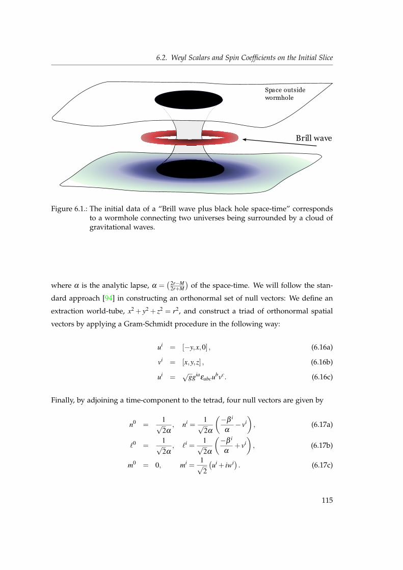
6.2. Weyl Scalars and Spin Coefficients on the Initial Slice
Space outside wormhole
Brill wave
Figure 6.1.: The initial data of a “Brill wave plus black hole space-time” correspondsto a wormhole connecting two universes being surrounded by a cloud ofgravitational waves.
where α is the analytic lapse, α =(2r−M
2r+M
)of the space-time. We will follow the stan-
dard approach [94] in constructing an orthonormal set of null vectors: We define an
extraction world-tube, x2 + y2 + z2 = r2, and construct a triad of orthonormal spatial
vectors by applying a Gram-Schmidt procedure in the following way:
ui = [−y,x,0] , (6.16a)
vi = [x,y,z] , (6.16b)
ui =√
ggiaεabcubvc. (6.16c)
Finally, by adjoining a time-component to the tetrad, four null vectors are given by
n0 =1√2α
, ni =1√2α
(−β i
α− vi
), (6.17a)
`0 =1√2α
, `i =1√2α
(−β i
α+ vi
), (6.17b)
m0 = 0, mi =1√2
(ui + iwi) . (6.17c)
115
6. Distorted Black Hole Space-Times in the NP Formalism
The explicit expression of the tetrad is
`µ
B =1√2
((2r +M)(2r−M)
,e−q
ψ2 ,0,0)
, (6.18a)
nµ
B =1√2
((2r +M)(2r−M)
,−e−q
ψ2 ,0,0)
, (6.18b)
mµ
B =1√2
(0,0,− e−q
rψ2 ,i
rψ2 sinθ
), (6.18c)
where the null vectors satisfy the null-vector conditions Eqs. (4.22, 4.22). The index B
indicates quantities on the initial slice.
The vectors in such a tetrad will differ from the expressions of the Kinnersley tetrad;
as a consequence, all quantities calculated in this frame will differ from the quantities
calculated in the Kinnersley tetrad as well. Most importantly, the Weyl scalars will all
be non-zero. For our particular choice of the metric these will result in
ΨB2 =
e−2q(r,θ)
S
(−6M−
(2r2(
∂ψ
∂ r
)2
−(
∂ψ
∂θ
)2)
M2+−2ψ
(3M±
(cot(θ)− ∂q
∂θ
)∂ψ
∂θ
+ 3M±ψ(0,2) + r
(6M2 +16rM−24r2 +3rM±
∂q∂ r
)∂ψ
∂ r
)M+
− ψ2(
8Mr(M +6r)−3M+
(M± cot(θ)
∂q∂θ− r(M2 +4rM−4r2) ∂q
∂ r
))), (6.19a)
ΨB1 =
3e−2q(r,θ)M+
S
(((M2 +4rM−4r2) ∂q
∂θ+ rM± cot(θ)
∂q∂ r
)ψ
2
+ 2(
∂ψ
∂θ
(M±+4rM + rM±
∂q∂ r
)+ rM±
(∂q∂θ
∂ψ
∂ r− ∂ 2ψ
∂ r∂θ
))ψ +6rM±
∂ψ
∂θ
∂ψ
∂ r
),
(6.19b)
ΨB4 =
3e−2q(r,θ)M+
S
((−M± cot(θ)
∂q∂θ
+M±∂ 2q∂θ 2 + r
(2(M±+2rM)
∂q∂ r
+ rM±∂ 2q∂ r2
))ψ
2
+ 2M±
(∂q∂ r
∂ψ
∂ rr2−
(cot(θ)+
∂q∂θ
)∂ψ
∂θ+
∂ 2ψ
∂θ 2
)ψ−6M±
(∂ψ
∂θ
)2)
, (6.19c)
where S =−12r2M−M2+ψ(r,θ)6 M± = M+M−, M+ = M +2r and M− = M−2r . The Weyl
116
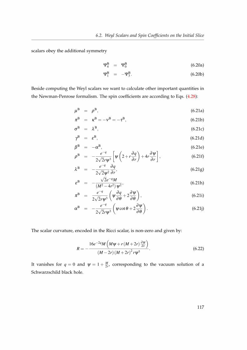
6.2. Weyl Scalars and Spin Coefficients on the Initial Slice
scalars obey the additional symmetry
ΨB4 = Ψ
B0 (6.20a)
ΨB1 = −Ψ
B3 . (6.20b)
Beside computing the Weyl scalars we want to calculate other important quantities in
the Newman-Penrose formalism. The spin coefficients are according to Eqs. (4.28):
µB = ρ
B, (6.21a)
πB = κ
B =−νB =−τ
B, (6.21b)
σB = λ
B, (6.21c)
γB = ε
B, (6.21d)
βB = −α
B, (6.21e)
ρB = − e−q
2√
2rψ3
[ψ
(2+ r
∂q∂ r
)+4r
∂ψ
∂ r
], (6.21f)
λB = − e−q
2√
2ψ2
∂q∂ r
, (6.21g)
εB = −
√2e−qM
(M2−4r2)ψ2 , (6.21h)
πB =
e−q
2√
2rψ3
(ψ
∂q∂θ
+2∂ψ
∂θ
), (6.21i)
αB = − e−q
2√
2rψ3
(ψ cotθ +2
∂ψ
∂θ
). (6.21j)
The scalar curvature, encoded in the Ricci scalar, is non-zero and given by:
R =−16e−2qM
(Mψ + r (M +2r) ∂ψ
∂ r
)(M−2r)(M +2r)2 rψ5
. (6.22)
It vanishes for q = 0 and ψ = 1 + M2r , corresponding to the vacuum solution of a
Schwarzschild black hole.
117
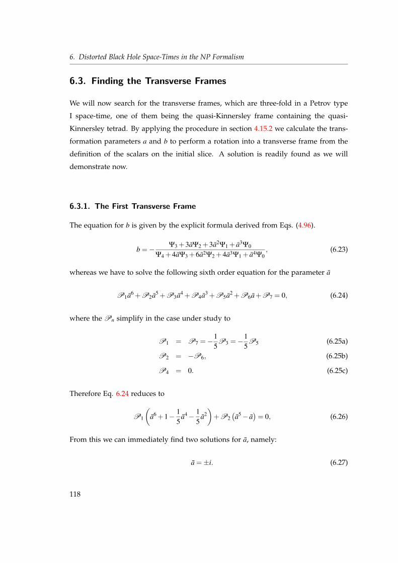
6. Distorted Black Hole Space-Times in the NP Formalism
6.3. Finding the Transverse Frames
We will now search for the transverse frames, which are three-fold in a Petrov type
I space-time, one of them being the quasi-Kinnersley frame containing the quasi-
Kinnersley tetrad. By applying the procedure in section 4.15.2 we calculate the trans-
formation parameters a and b to perform a rotation into a transverse frame from the
definition of the scalars on the initial slice. A solution is readily found as we will
demonstrate now.
6.3.1. The First Transverse Frame
The equation for b is given by the explicit formula derived from Eqs. (4.96).
b =− Ψ3 +3aΨ2 +3a2Ψ1 + a3Ψ0
Ψ4 +4aΨ3 +6a2Ψ2 +4a3Ψ1 + a4Ψ0, (6.23)
whereas we have to solve the following sixth order equation for the parameter a
P1a6 +P2a5 +P3a4 +P4a3 +P5a2 +P6a+P7 = 0, (6.24)
where the Pn simplify in the case under study to
P1 = P7 =−15P3 =−1
5P5 (6.25a)
P2 = −P6, (6.25b)
P4 = 0. (6.25c)
Therefore Eq. 6.24 reduces to
P1
(a6 +1− 1
5a4− 1
5a2)
+P2(a5− a
)= 0, (6.26)
From this we can immediately find two solutions for a, namely:
a =±i. (6.27)
118
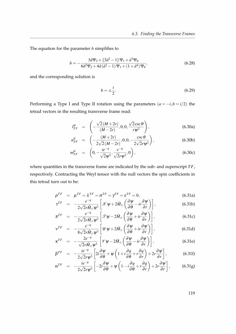
6.3. Finding the Transverse Frames
The equation for the parameter b simplifies to
b =−3aΨ2 +
(3a2−1
)Ψ1 + a3Ψ0
6a2Ψ2 +4a(a2−1)Ψ1 +(1+ a4)Ψ0, (6.28)
and the corresponding solution is
b =± i2. (6.29)
Performing a Type I and Type II rotation using the parameters (a =−i,b = i/2) the
tetrad vectors in the resulting transverse frame read:
lµ
T F =
(−√
2(M +2r)(M−2r)
,0,0,
√2cscθ
rψ2
), (6.30a)
nµ
T F =(− (M +2r)
2√
2(M−2r),0,0,− cscθ
2√
2rψ2
), (6.30b)
mµ
T F =(
0,− ie−q√
2ψ2,
e−q√
2rψ2,0)
, (6.30c)
where quantities in the transverse frame are indicated by the sub- and superscript T F ,
respectively. Contracting the Weyl tensor with the null vectors the spin coefficients in
this tetrad turn out to be:
ρT F = µ
T F = λT F = σ
T F = γT F = ε
T F = 0, (6.31a)
τT F = − e−q
2√
2rM±ψ3
[X ψ +2M±
(∂ψ
∂θ− ir
∂ψ
∂ r
)], (6.31b)
πT F = − e−q
2√
2rM±ψ3
[T ψ−2M±
(∂ψ
∂θ+ ir
∂ψ
∂ r
)], (6.31c)
νT F = − e−q
8√
2rM±ψ3
[U ψ +2M±
(∂ψ
∂θ+ ir
∂ψ
∂ r
)], (6.31d)
κT F = − 2e−q
√2rM±ψ3
[V ψ−2M±
(∂ψ
∂θ− ir
∂ψ
∂ r
)], (6.31e)
βT F = − ie−q
2√
2rψ3
[2i
∂ψ
∂θ+ψ
(1+ i
∂q∂θ
+ r∂q∂ r
)+2r
∂ψ
∂ r
], (6.31f)
αT F = − ie−q
2√
2rψ3
[−2i
∂ψ
∂θ+ψ
(1− i
∂q∂θ
+ r∂q∂ r
)+2r
∂ψ
∂ r
], (6.31g)
119
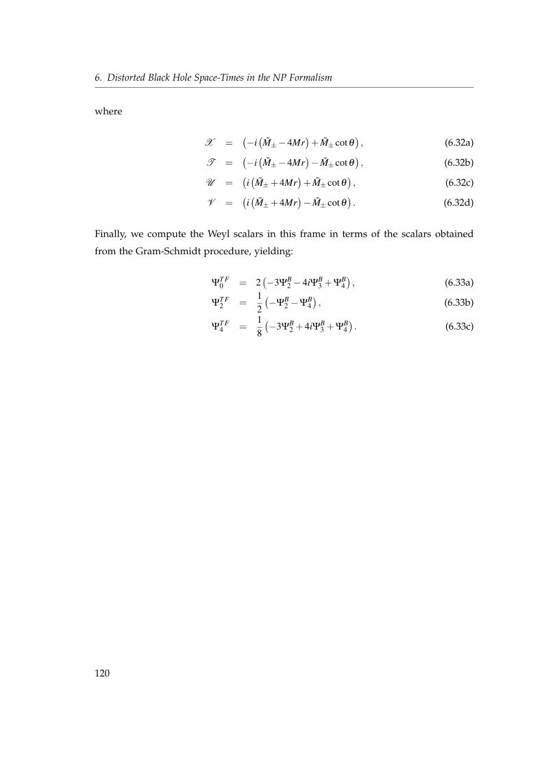
6. Distorted Black Hole Space-Times in the NP Formalism
where
X =(−i(M±−4Mr
)+ M± cotθ
), (6.32a)
T =(−i(M±−4Mr
)− M± cotθ
), (6.32b)
U =(i(M±+4Mr
)+ M± cotθ
), (6.32c)
V =(i(M±+4Mr
)− M± cotθ
). (6.32d)
Finally, we compute the Weyl scalars in this frame in terms of the scalars obtained
from the Gram-Schmidt procedure, yielding:
ΨT F0 = 2
(−3Ψ
B2 −4iΨB
3 +ΨB4), (6.33a)
ΨT F2 =
12(−Ψ
B2 −Ψ
B4), (6.33b)
ΨT F4 =
18(−3Ψ
B2 +4iΨB
3 +ΨB4). (6.33c)
120
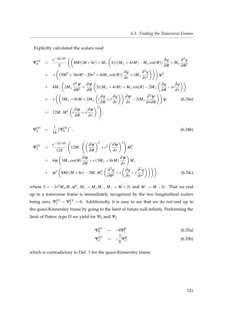
6.3. Finding the Transverse Frames
Explicitly calculated the scalars read
ΨT F0 =
e−2q(r,θ)
S
((8Mr(M +6r)+M+
(4(i(M±+4rM)−M± cot(θ))
∂q∂θ
+M±∂ 2q∂θ 2
+ r((
5M2 +16rM−20r2 +4iM± cot(θ)) ∂q
∂ r+ rM±
∂ 2q∂ r2
)))ψ
2
+ 4M+
(2M±
∂ 2ψ
∂θ 2 +∂ψ
∂θ
(2i(M±+4rM)+M± cot(θ)−2M±
(∂q∂θ− ir
∂q∂ r
))+ r
((3M±+8rM +2M±
(i∂q∂θ
+ r∂q∂ r
))∂ψ
∂ r−2iM±
∂ 2ψ
∂ r∂θ
))ψ (6.34a)
+ 12M−M2+
(i∂ψ
∂θ+ r
∂ψ
∂ r
)2)
,
ΨT F4 =
116(Ψ
T F0)∗
, (6.34b)
ΨT F2 =
e−2q(r,θ)
12S
(12M−
((∂ψ
∂θ
)2
+ r2(
∂ψ
∂ r
)2)
M2+
+ 4ψ
(3M± cot(θ)
∂ψ
∂θ+ r (3M±+8rM)
∂ψ
∂ r
)M+
+ ψ2(
8Mr(M +6r)−3M−M2+
(∂ 2q∂θ 2 + r
(∂q∂ r
+ r∂ 2q∂ r2
)))), (6.34c)
where S = −2r2M±M+ψ6, M± = M+M−, M+ = M + 2r and M− = M− 2r. That we end
up in a transverse frame is immediately recognized by the two longitudinal scalars
being zero, ΨT F1 = ΨT F
3 = 0. Additionally, it is easy to see that we do not end up in
the quasi-Kinnersley frame by going to the limit of future null infinity. Performing the
limit of Petrov type D we yield for Ψ0 and Ψ4
ΨT F0 → −6Ψ
B2 (6.35a)
ΨT F4 → −3
8Ψ
B2 , (6.35b)
which is contradictory to Def. 3 for the quasi-Kinnersley frame.
121
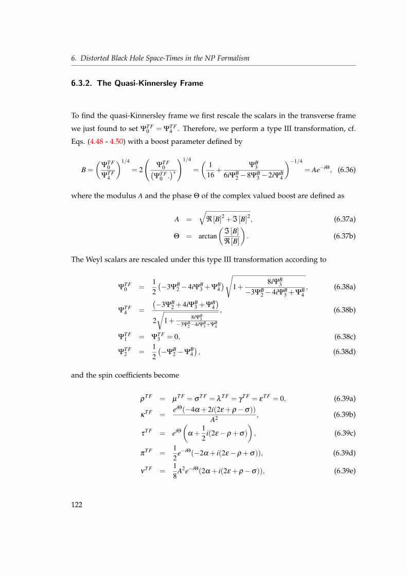
6. Distorted Black Hole Space-Times in the NP Formalism
6.3.2. The Quasi-Kinnersley Frame
To find the quasi-Kinnersley frame we first rescale the scalars in the transverse frame
we just found to set ΨT F0 = ΨT F
4 . Therefore, we perform a type III transformation, cf.
Eqs. (4.48 - 4.50) with a boost parameter defined by
B =(
ΨT F0
ΨT F4
)1/4
= 2
(ΨT F
0(ΨT F
0 .)∗)1/4
=(
116
+ΨB
3
6iΨB2 −8ΨB
3 −2iΨB4
)−1/4
= Ae−iΘ, (6.36)
where the modulus A and the phase Θ of the complex valued boost are defined as
A =√
ℜ [B]2 +ℑ [B]2, (6.37a)
Θ = arctan(
ℑ [B]ℜ [B]
). (6.37b)
The Weyl scalars are rescaled under this type III transformation according to
ΨT F0 =
12(−3Ψ
B2 −4iΨB
3 +ΨB4)√
1+8iΨB
3
−3ΨB2 −4iΨB
3 +ΨB4, (6.38a)
ΨT F4 =
(−3ΨB
2 +4iΨB3 +ΨB
4)
2√
1+ 8iΨB3
−3ΨB2−4iΨB
3 +ΨB4
, (6.38b)
ΨT F1 = Ψ
T F3 = 0, (6.38c)
ΨT F2 =
12(−Ψ
B2 −Ψ
B4), (6.38d)
and the spin coefficients become
ρT F = µ
T F = σT F = λ
T F = γT F = ε
T F = 0, (6.39a)
κT F =
eiΘ(−4α +2i(2ε +ρ−σ))A2 , (6.39b)
τT F = eiΘ
(α +
12
i(2ε−ρ +σ))
, (6.39c)
πT F =
12
e−iΘ(−2α + i(2ε−ρ +σ)), (6.39d)
νT F =
18
A2e−iΘ(2α + i(2ε +ρ−σ)), (6.39e)
122
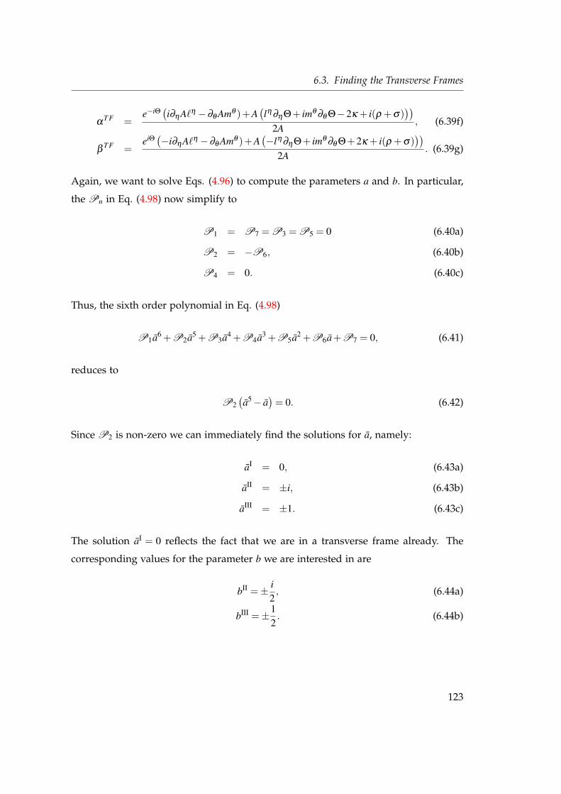
6.3. Finding the Transverse Frames
αT F =
e−iΘ(i∂ηA`η −∂θ Amθ )+A
(lη∂ηΘ+ imθ ∂θ Θ−2κ + i(ρ +σ)
))2A
, (6.39f)
βT F =
eiΘ(−i∂ηA`η −∂θ Amθ )+A
(−lη∂ηΘ+ imθ ∂θ Θ+2κ + i(ρ +σ)
))2A
. (6.39g)
Again, we want to solve Eqs. (4.96) to compute the parameters a and b. In particular,
the Pn in Eq. (4.98) now simplify to
P1 = P7 = P3 = P5 = 0 (6.40a)
P2 = −P6, (6.40b)
P4 = 0. (6.40c)
Thus, the sixth order polynomial in Eq. (4.98)
P1a6 +P2a5 +P3a4 +P4a3 +P5a2 +P6a+P7 = 0, (6.41)
reduces to
P2(a5− a
)= 0. (6.42)
Since P2 is non-zero we can immediately find the solutions for a, namely:
aI = 0, (6.43a)
aII = ±i, (6.43b)
aIII = ±1. (6.43c)
The solution aI = 0 reflects the fact that we are in a transverse frame already. The
corresponding values for the parameter b we are interested in are
bII =± i2, (6.44a)
bIII =±12. (6.44b)
123
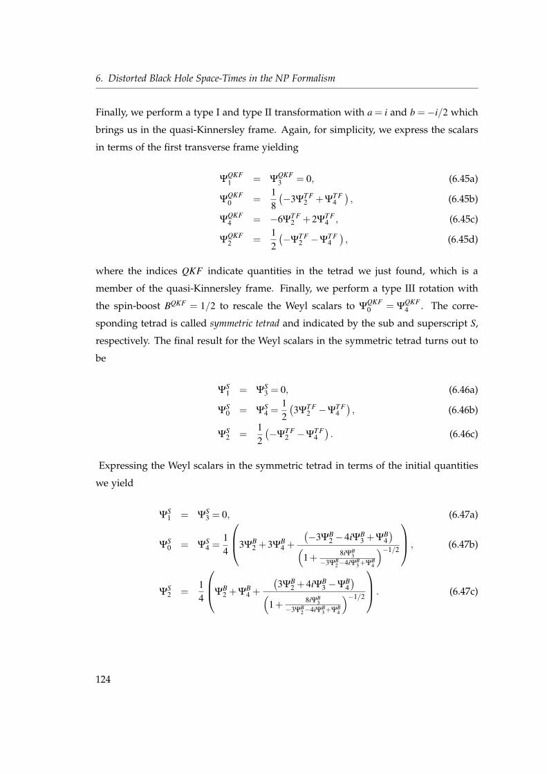
6. Distorted Black Hole Space-Times in the NP Formalism
Finally, we perform a type I and type II transformation with a = i and b =−i/2 which
brings us in the quasi-Kinnersley frame. Again, for simplicity, we express the scalars
in terms of the first transverse frame yielding
ΨQKF1 = Ψ
QKF3 = 0, (6.45a)
ΨQKF0 =
18(−3Ψ
T F2 +Ψ
T F4), (6.45b)
ΨQKF4 = −6Ψ
T F2 +2Ψ
T F4 , (6.45c)
ΨQKF2 =
12(−Ψ
T F2 −Ψ
T F4), (6.45d)
where the indices QKF indicate quantities in the tetrad we just found, which is a
member of the quasi-Kinnersley frame. Finally, we perform a type III rotation with
the spin-boost BQKF = 1/2 to rescale the Weyl scalars to ΨQKF0 = Ψ
QKF4 . The corre-
sponding tetrad is called symmetric tetrad and indicated by the sub and superscript S,
respectively. The final result for the Weyl scalars in the symmetric tetrad turns out to
be
ΨS1 = Ψ
S3 = 0, (6.46a)
ΨS0 = Ψ
S4 =
12(3Ψ
T F2 −Ψ
T F4), (6.46b)
ΨS2 =
12(−Ψ
T F2 −Ψ
T F4). (6.46c)
Expressing the Weyl scalars in the symmetric tetrad in terms of the initial quantities
we yield
ΨS1 = Ψ
S3 = 0, (6.47a)
ΨS0 = Ψ
S4 =
14
3ΨB2 +3Ψ
B4 +
(−3ΨB
2 −4iΨB3 +ΨB
4)(
1+ 8iΨB3
−3ΨB2−4iΨB
3 +ΨB4
)−1/2
, (6.47b)
ΨS2 =
14
ΨB2 +Ψ
B4 +
(3ΨB
2 +4iΨB3 −ΨB
4)(
1+ 8iΨB3
−3ΨB2−4iΨB
3 +ΨB4
)−1/2
. (6.47c)
124
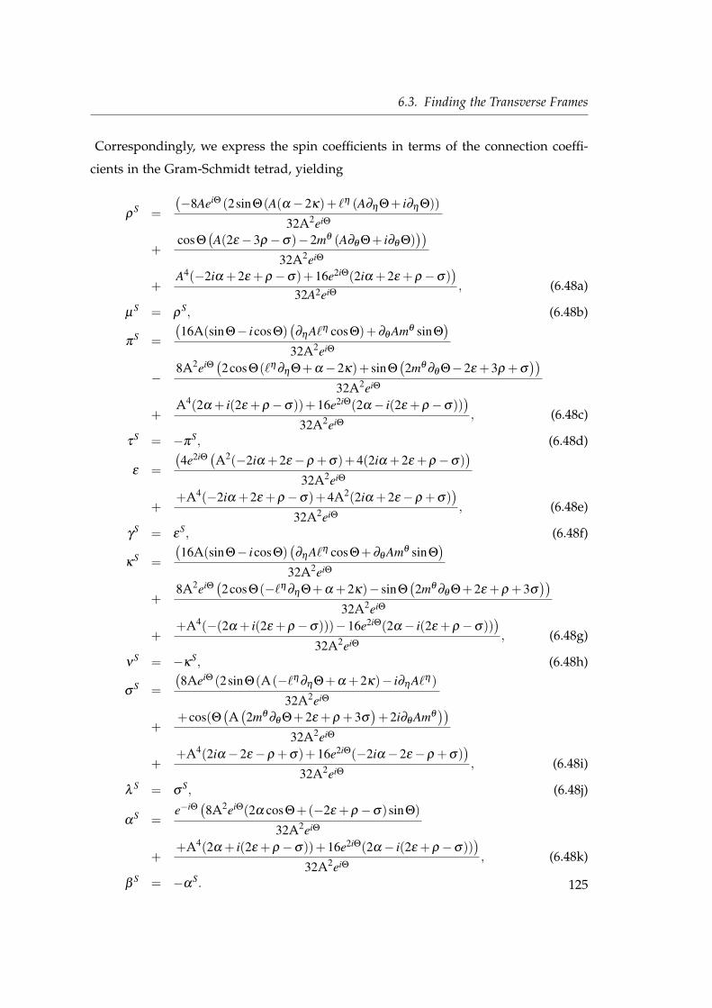
6.3. Finding the Transverse Frames
Correspondingly, we express the spin coefficients in terms of the connection coeffi-
cients in the Gram-Schmidt tetrad, yielding
ρS =
(−8AeiΘ (2sinΘ(A(α−2κ)+ `η (A∂ηΘ+ i∂ηΘ))
32A2eiΘ
+cosΘ
(A(2ε−3ρ−σ)−2mθ (A∂θ Θ+ i∂θ Θ)
))32A2eiΘ
+A4(−2iα +2ε +ρ−σ)+16e2iΘ(2iα +2ε +ρ−σ)
)32A2eiΘ , (6.48a)
µS = ρ
S, (6.48b)
πS =
(16A(sinΘ− icosΘ)
(∂ηA`η cosΘ)+∂θ Amθ sinΘ
)32A2eiΘ
−8A2eiΘ
(2cosΘ(`η∂ηΘ+α−2κ)+ sinΘ
(2mθ ∂θ Θ−2ε +3ρ +σ
))32A2eiΘ
+A4(2α + i(2ε +ρ−σ))+16e2iΘ(2α− i(2ε +ρ−σ))
)32A2eiΘ
, (6.48c)
τS = −π
S, (6.48d)
ε =
(4e2iΘ
(A2(−2iα +2ε−ρ +σ)+4(2iα +2ε +ρ−σ)
)32A2eiΘ
++A4(−2iα +2ε +ρ−σ)+4A2(2iα +2ε−ρ +σ)
)32A2eiΘ
, (6.48e)
γS = ε
S, (6.48f)
κS =
(16A(sinΘ− icosΘ)
(∂ηA`η cosΘ+∂θ Amθ sinΘ
)32A2eiΘ
+8A2eiΘ
(2cosΘ(−`η∂ηΘ+α +2κ)− sinΘ
(2mθ ∂θ Θ+2ε +ρ +3σ
))32A2eiΘ
++A4(−(2α + i(2ε +ρ−σ)))−16e2iΘ(2α− i(2ε +ρ−σ))
)32A2eiΘ
, (6.48g)
νS = −κ
S, (6.48h)
σS =
(8AeiΘ (2sinΘ(A(−`η∂ηΘ+α +2κ)− i∂ηA`η)
32A2eiΘ
++cos(Θ
(A(2mθ ∂θ Θ+2ε +ρ +3σ
)+2i∂θ Amθ
))32A2eiΘ
++A4(2iα−2ε−ρ +σ)+16e2iΘ(−2iα−2ε−ρ +σ)
)32A2eiΘ
, (6.48i)
λS = σ
S, (6.48j)
αS =
e−iΘ(8A2eiΘ(2α cosΘ+(−2ε +ρ−σ)sinΘ)
32A2eiΘ
++A4(2α + i(2ε +ρ−σ))+16e2iΘ(2α− i(2ε +ρ−σ))
)32A2eiΘ
, (6.48k)
βS = −α
S. 125
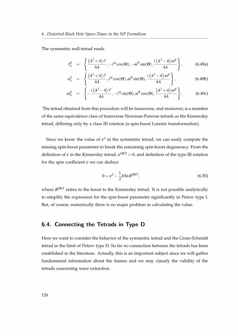
6. Distorted Black Hole Space-Times in the NP Formalism
The symmetric null-tetrad reads
`µ
S =
(A2 +4
)`t
4A,−`η cos(Θ),−mθ sin(Θ),
i(A2−4
)mφ
4A
, (6.49a)
nµ
S =
(A2 +4
)`t
4A, `η cos(Θ),mθ sin(Θ),
i(A2−4
)mφ
4A
, (6.49b)
mµ
S =
−
i(A2−4
)`t
4A,−`η sin(Θ),mθ cos(Θ),
(A2 +4
)mφ
4A
. (6.49c)
The tetrad obtained from this procedure will be transverse, and moreover, is a member
of the same equivalence class of transverse Newman-Penrose tetrads as the Kinnersley
tetrad, differing only by a class III rotation (a spin-boost Lorentz transformation).
Since we know the value of εS in the symmetric tetrad, we can easily compute the
missing spin-boost parameter to break the remaining spin-boost degeneracy. From the
definition of ε in the Kinnersley tetrad, εQKT = 0, and definition of the type III rotation
for the spin coefficient ε we can deduce
0 = εS− 1
2D lnBQKT, (6.50)
where BQKT refers to the boost to the Kinnersley tetrad. It is not possible analytically
to simplify the expression for the spin-boost parameter significantly in Petrov type I.
But, of course, numerically there is no major problem in calculating the value.
6.4. Connecting the Tetrads in Type D
Here we want to consider the behavior of the symmetric tetrad and the Gram-Schmidt
tetrad in the limit of Petrov type D. So far no connection between the tetrads has been
established in the literature. Actually, this is an important subject since we will gather
fundamental information about the frames and we may classify the validity of the
tetrads concerning wave extraction.
126
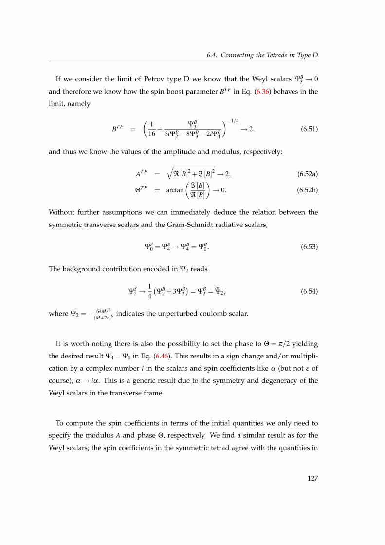
6.4. Connecting the Tetrads in Type D
If we consider the limit of Petrov type D we know that the Weyl scalars ΨB3 → 0
and therefore we know how the spin-boost parameter BT F in Eq. (6.36) behaves in the
limit, namely
BT F =(
116
+ΨB
3
6iΨB2 −8ΨB
3 −2iΨB4
)−1/4
→ 2, (6.51)
and thus we know the values of the amplitude and modulus, respectively:
AT F =√
ℜ [B]2 +ℑ [B]2→ 2, (6.52a)
ΘT F = arctan
(ℑ [B]ℜ [B]
)→ 0. (6.52b)
Without further assumptions we can immediately deduce the relation between the
symmetric transverse scalars and the Gram-Schmidt radiative scalars,
ΨS0 = Ψ
S4→Ψ
B4 = Ψ
B0 . (6.53)
The background contribution encoded in Ψ2 reads
ΨS2→
14(Ψ
B2 +3Ψ
B2)
= ΨB2 = Ψ2, (6.54)
where Ψ2 =− 64Mr3
(M+2r)6 indicates the unperturbed coulomb scalar.
It is worth noting there is also the possibility to set the phase to Θ = π/2 yielding
the desired result Ψ4 = Ψ0 in Eq. (6.46). This results in a sign change and/or multipli-
cation by a complex number i in the scalars and spin coefficients like α (but not ε of
course), α → iα . This is a generic result due to the symmetry and degeneracy of the
Weyl scalars in the transverse frame.
To compute the spin coefficients in terms of the initial quantities we only need to
specify the modulus A and phase Θ, respectively. We find a similar result as for the
Weyl scalars; the spin coefficients in the symmetric tetrad agree with the quantities in
127
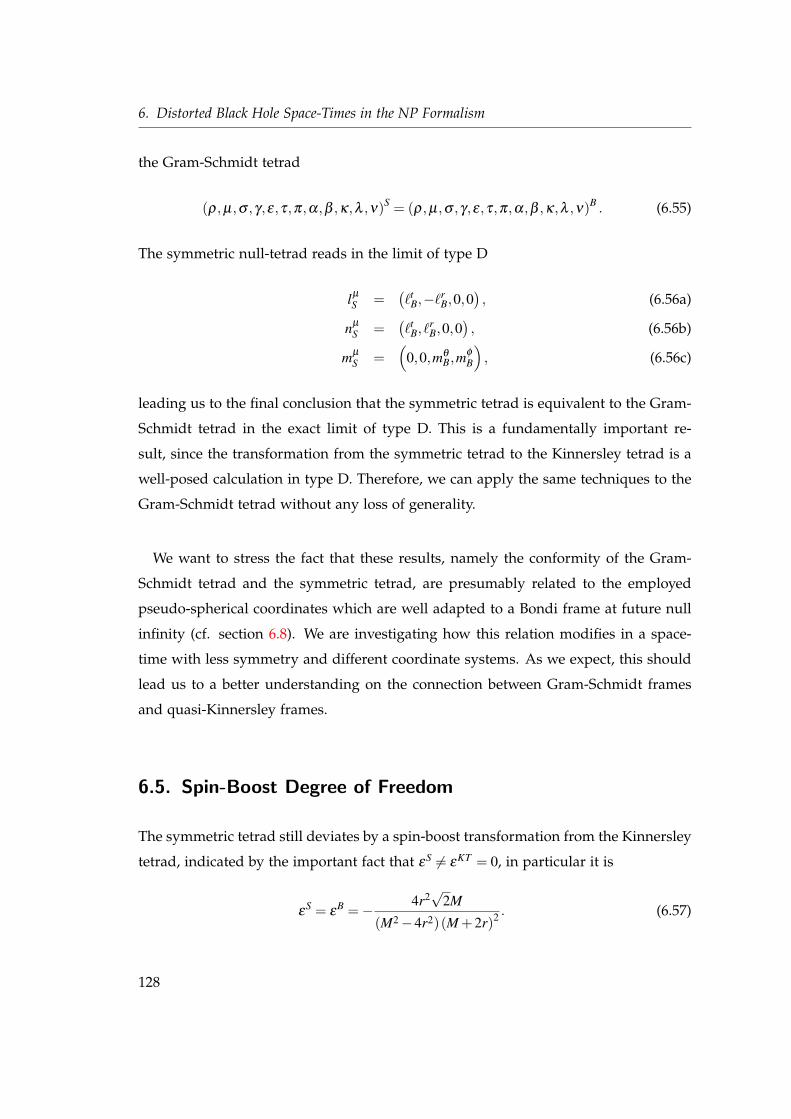
6. Distorted Black Hole Space-Times in the NP Formalism
the Gram-Schmidt tetrad
(ρ,µ,σ ,γ,ε,τ,π,α,β ,κ,λ ,ν)S = (ρ,µ,σ ,γ,ε,τ,π,α,β ,κ,λ ,ν)B . (6.55)
The symmetric null-tetrad reads in the limit of type D
lµ
S =(`t
B,−`rB,0,0
), (6.56a)
nµ
S =(`t
B, `rB,0,0
), (6.56b)
mµ
S =(
0,0,mθB,mφ
B
), (6.56c)
leading us to the final conclusion that the symmetric tetrad is equivalent to the Gram-
Schmidt tetrad in the exact limit of type D. This is a fundamentally important re-
sult, since the transformation from the symmetric tetrad to the Kinnersley tetrad is a
well-posed calculation in type D. Therefore, we can apply the same techniques to the
Gram-Schmidt tetrad without any loss of generality.
We want to stress the fact that these results, namely the conformity of the Gram-
Schmidt tetrad and the symmetric tetrad, are presumably related to the employed
pseudo-spherical coordinates which are well adapted to a Bondi frame at future null
infinity (cf. section 6.8). We are investigating how this relation modifies in a space-
time with less symmetry and different coordinate systems. As we expect, this should
lead us to a better understanding on the connection between Gram-Schmidt frames
and quasi-Kinnersley frames.
6.5. Spin-Boost Degree of Freedom
The symmetric tetrad still deviates by a spin-boost transformation from the Kinnersley
tetrad, indicated by the important fact that εS 6= εKT = 0, in particular it is
εS = ε
B =− 4r2√
2M
(M2−4r2)(M +2r)2 . (6.57)
128
6.5. Spin-Boost Degree of Freedom
By comparing the values of the spin coefficients in the two tetrads of interest it turns
out that αS, β S, τS and πS already agree with the value in the Kinnersley tetrad and
therefore we can further constrain the unknown spin-boost parameter. Using Eqs.
(4.50f, 4.50g, 4.50k, 4.50l)
τKT = eiΘSτ
S, (6.58a)
πKT = e−iΘSπ
S, (6.58b)
αIII = e−iΘSα− 1
2A−1
S e−iΘSδ∗AS +
12
ie−iΘSδ∗ΘS, (6.58c)
βIII = eiΘSβ − 1
2A−1
S eiΘSδAS +12
ieiΘSδΘ, (6.58d)
we can not only conclude that the phase ΘS is constant but, in fact, is equal to zero.
Additionally we can conclude that AS does not depend on t and φ , thus
AS = AS (r,θ) . (6.59)
The next step is to determine the exact expression of the amplitude AS (r,θ) to per-
form a type III transformation in the Kinnersley tetrad. The starting point will be the
equation for the spin coefficient ε in the quasi-Kinnersley frame
0 =1
ASε
S− 12
(AS)−2 DAS, (6.60)
where the directional derivative is defined as D = `µ
S ∂µ and the left hand side corre-
sponds to the value for the spin coefficient in the Kinnersley tetrad, εKT = 0. We may
solve this equation for AS:
εS =
12
D logAS, (6.61)
where a straightforward calculation yields the desired result for the transformation:
AS = BS = D(M−2r)(M +2r)
, (6.62)
129
6. Distorted Black Hole Space-Times in the NP Formalism
with a yet to be determined integration constant. Such a transformation will leave the
scalar Ψ2 unchanged, but will have in general a strong effect on the radiative quanti-
ties Ψ0 and Ψ4, scaling and mixing polarizations.
We can not constrain the spin-boost parameter from the spin coefficient ε any fur-
ther. For this we make use of the spin coefficients γ . The type III transformation
equation for γ is
γKT = AS
γS− 1
2∆AS, (6.63)
fixing the integration constant to D = −1/√
2. The final result for the spin-boost pa-
rameter BS reads
BS =− (M−2r)√2(M +2r)
. (6.64)
We compare the value we achieve for the boost with the more general definition we
derived in chapter 5, Eq. (5.48), where the function H encodes all information of the
Weyl scalars and spin coefficients in the transverse frames,
∇µ
∇µH +∇µ ln(
I16
)∇µ
(2H + ln I
112
)=−2Ψ2. (6.65)
In the limit of a single black hole, Eq.(6.65) is immediately solvable, leading us to the
following condition on the spin-boost parameter (cf. Eq. (5.60))
B = B0I16 Γ
12 . (6.66)
We perform a suitable transformation to adapt the result to our particular coordinate
system yielding for Eq. (6.66)
B = B0
(√3M)(1/3) (M−2r)
(M +2r). (6.67)
Comparing Eq. (6.64) and Eq. (6.67) we can determine the remaining constant of
130
6.5. Spin-Boost Degree of Freedom
integration B0, yielding
B−10 =−
√2(√
3M)1/3
. (6.68)
Whether this is a generic result or a particular value of the space-time under consider-
ation is not yet fully determined. The calculation of B0 from a more theoretical point
of view is still under investigation and will be published elsewhere.
Since we end up in the Kinnersley tetrad after performing a boost with BS =− (M−2r)√2(M+2r)
all spin coefficients have the correct value for the vacuum solution of a non-rotating
black hole in isotropic coordinates:
ε = τ = ν = κ = π = σ = λ = 0, (6.69a)
γ =8Mr2
(M +2r)4 , (6.69b)
ρ = − 4r
(M +2r)2 , (6.69c)
µ =12
ρ +2γ, (6.69d)
β = −α =√
2r cotθ
(M +2r)2 . (6.69e)
The tetrad agrees with the well-known expressions of the Kinnersley tetrad:
˜µ =
((M +2r)2
(M−2r)2 ,− 4r2
(M2−4r2),0,0
), (6.70a)
nµ =
(12,2r2 (M−2r)(M +2r)3 ,0,0
), (6.70b)
mµ =
(0,0,
2√
2r
(M +2r)2 ,2√
2ir cscθ
(M +2r)2
). (6.70c)
131
6. Distorted Black Hole Space-Times in the NP Formalism
6.6. Perturbation Theory for the Close Limit
In this section we provide the basic mathematical formalism for evolving distorted
black holes as perturbative systems. We investigate the multipole moments of a gen-
eral space-time as a linear perturbation about its background spherical part. Roughly
speaking, this approach should be a valid way to describe black hole space-times,
whose non-spherical departure from Schwarzschild is small. We are particularly in-
terested in the radial fall-off of the Weyl scalars in the quasi-Kinnersley tetrad and the
Gram-Schmidt tetrad in the limit of Type D, respectively. In the foregoing sections we
have already deduced all expressions for the quantities in Petrov type I for both of the
tetrads. To receive explicit expressions for the radiative scalars we need to specify the
perturbation encoded in the function q. A suitable approach for such a task is per-
turbation theory. Our starting point for the perturbation analysis is the Hamiltonian
constraint in Eq. (6.14):
1r2
∂
∂ r
(r2 ∂
∂ r
)ψ +
1r2 sinθ
∂
∂θ
(sinθ
∂
∂θ
)ψ =−1
4ψ
(∂ 2q∂ r2 +
1r2
∂ 2q∂θ 2 +
1r
∂q∂ r
). (6.71)
In the literature the Brill waves have been repeatedly invoked as a tool for wave ex-
traction. The perturbation q = q(r,θ) has to satisfy a set of boundary conditions, but
is an otherwise arbitrary function. We follow [77, 85] and assume that q(r,θ) decays
fairly rapidly at infinity (at least as 1/r2) and that it is regular at θ = 0:
∂q(r,θ)∂θ
∣∣∣∣θ=0
= 0, limr→∞
q(r,θ) = O(r−2) , q(r,θ)
∣∣∣∣θ=0
= 0. (6.72)
In case of a superposition of a black hole and Brill waves we impose an additional
boundary condition at the throat of the Einstein-Rosen bridge. We choose the initial
slice to be isometric at the throat. The inversion-through-the-sphere transformation
from a point r > χ to a point inside the throat r < χ is given by [85]
r′ = χ2/r. (6.73)
From the usual tensor transformation rule for the metric component γ11,
132
6.6. Perturbation Theory for the Close Limit
γ′11(r′ = χ
)= γ11 (r = χ) , (6.74)
we can determine the throat condition on the isometry surface (assuming continuity
of the first derivate) [∂γ11
∂ r+
2γ11
χ
]r=χ
= 0. (6.75)
The most natural choice would be to choose the conformal factor to have the same con-
dition as in the unperturbed Schwarzschild solution. It turned out that this conditions
introduces numerical and analytical complications for the function q(r,θ). Therefore
we will perform a coordinate transformation to make use of a widely used system of
coordinates for the Brill waves, the η-coordinates [83, 84, 95, 85, 96] . The coordinate
transformation of the form
r =M2
eη (6.76)
was motivated by numerical reasons initially. The isometry constraint suffers from
the fact that it is a so called “anti-Robin” condition: it has the wrong relative sign
since the normal vector points in the wrong direction relative to the inner boundary.
This behavior is not suitable for the standard proofs of uniqueness for the initial-value
problem and may introduce problems with techniques for solving elliptic equations
(see [88, 85]) . We have encountered the same issue in a preceding work (Elbracht et
al. [97]).
In the new coordinates the line element, Eq. (6.15), now takes the form
ds2 =−(
eη −1eη +1
)2
dt2 +ψ(η)4 [e2q (dη2 + dθ
)+ sin2
θ dφ], (6.77)
and the Hamiltonian constraint, Eq. (6.14), is transformed into
∂2ηψ +∇
2θ ψ + cotθ∂θ ψ +
14
ψ(∂
2ηq+∂
2θ q−1
)= 0. (6.78)
133
6. Distorted Black Hole Space-Times in the NP Formalism
The inversion-through-the-sphere condition, Eq. (6.73), is now given by
η′ =−η . (6.79)
The throat condition on the isometry surface, Eq. (6.75), transforms into[∂γ11
∂η
]η=0
=[
∂q∂η
+2ψ
∂ψ
∂η
]η=0
= 0. (6.80)
We choose ψ to have the same boundary conditions as in the Schwarzschild solution,
namely
∂ψ
∂θ
∣∣∣∣θ=0
=∂ψ
∂θ
∣∣∣∣θ=π/2
=∂ψ
∂η
∣∣∣∣η=0
= 0, (6.81)
which determines the conditions for the perturbation q to
∂q∂θ
∣∣∣∣θ=0
=∂q∂θ
∣∣∣∣θ=π/2
=∂q∂η
∣∣∣∣η=0
= 0, (6.82)
therefore decoupling the boundary conditions for the conformal factor and the per-
turbation. By imposing an outer boundary condition ψ(η) is fixed completely.
The elliptic equation for the Hamiltonian constraint in Eq. (6.78) must in general be
solved numerically. Once this is done, it can be used to compute initial data for the
perturbation equations as described in the foregoing sections and can also be evolved
with a numerical code (see e.g. Elbracht et al [97]). Here we focus on the extraction
of initial data itself, not on the evolution. We expand the conformal factor and the
function q(r,θ) appearing in this equation in terms of spherical harmonics Ylm (θ ,φ)
such that
ψ (η ,θ ,φ) = ψ (η)+a∞
∑l=0
l
∑m=−l
ψlm (η)Ylm (θ ,φ)+O(a2) , (6.83)
with ψ (η) =√
2M cosh(
η
2
)being the conformal factor of the Schwarzschild solution.
134
6.6. Perturbation Theory for the Close Limit
The perturbation to linear order in a is
q(η ,θ ,φ) = a ∑l=2,4...
qlm (η)Ylm (θ ,φ) , (6.84)
where we further assume a < 1 which is a reasonable assumption considering the
amplitude of the wave. We construct a perturbation q in the following manner
q(η ,θ) =√
π
58aq(η)
(−1
3Y20 +
√5
3Y00
)= 2ae−η2
sin2θ , (6.85)
satisfying the boundary conditions in Eq. (6.82). We may now solve the Hamiltonian
constraint with that particular perturbation. The only non-zero coefficients of the
conformal factor in the first-order expansion are
ψ00 =13
√2√
Me−η2(
πeη2(
erf(η)sinh(
η
2
)− cosh
(η
2
))−2√
π cosh(
η
2
)), (6.86a)
ψ20 =13
√2π
5
√Me−
12 η(2η+5)
(−√
πeη2+ 94 + e2η + e3η
)+
π√
Me94−
5η
2(erfc
(η− 3
2
)− e5ηerfc
(η + 3
2
))3√
10, (6.86b)
where erf(η) and erfc(η) are the error function and complementary error function,
respectively. All terms with m 6= 0 vanish due to the imposed azimuthal symmetry.
We end up not only with an angular contribution from the Y20 spherical harmonic but
additionally we get a Y00-term. This is a particular effect caused by the way we have
constructed the perturbation. We have now all necessary information to calculate the
radiative scalars and spin coefficients in the two tetrads under investigation.
6.6.1. Perturbed Newman-Penrose Quantities in the Gram-Schmidt Tetrad
We will use the exact analytic solution to the perturbative initial data equations to
discuss a specific example of the extraction procedure applied to the axisymmetric
black hole initial data sets discussed above. We construct the perturbed null vectors
in the same way as in section 6.2, Eqs. (6.16, 6.17), still satisfying to linear order the
135
6. Distorted Black Hole Space-Times in the NP Formalism
null-vector conditions (cf. Eqs. (4.22, 4.22))
`µ`µ = mµmµ = 0, (6.87a)
`µnµ = mµmµ = 1. (6.87b)
Contracting the Weyl tensor with the perturbed vectors yields for the spin coefficients
ρB = −
2√
2sinh4 (η
2
)csch3(η)
M− 4√
2πQe−2η
3M, (6.88a)
µB = ρ
B, (6.88b)
τB = −
√2Qe−η2
sin(2θ)M
, (6.88c)
πB = −τ
B, (6.88d)
λB =
2√
2Qe−η2η sin2(θ)
M, (6.88e)
σB = λ
B, (6.88f)
νB = τ
B, (6.88g)
κB = −τ
B, (6.88h)
γB =
sinh2 (η
2
)csch3(η)
√2M
+2√
2πQe−5η
3M, (6.88i)
βB =
sech2 (η
2
)cot(θ)
4√
2M+√
2πQe−2η cot(θ)3M
, (6.88j)
αB = −β
B, (6.88k)
εB = γ
B. (6.88l)
The Weyl scalars to linear order in a read
Ψ0 = Ψ4 =2√
πae−5η sin2θ
M2 , (6.89a)
Ψ1 = −Ψ3 =4√
πae−5η sin(2θ)M2 , (6.89b)
136
6.6. Perturbation Theory for the Close Limit
and the correction in leading order to the background is
Ψ2 = Ψ2 +4√
πae−3η
3M2 , (6.90)
where Ψ2 = − 18M2 sech6 (η/2) is the Schwarzschild solution and the scalars still obey
the symmetry
ΨB0 −Ψ
B4 = 0+O
[a2] , (6.91a)
ΨB1 +Ψ
B3 = 0+O
[a2] . (6.91b)
6.6.2. Perturbed Newman-Penrose Quantities in the Symmetric Tetrad
Making use of Eqs. (6.47) the calculation of the Weyl scalars in the symmetric tetrad
in Petrov type D is a straightforward task, yielding
ΨS0 = Ψ
B0 +O
(a2) , (6.92a)
ΨS4 = Ψ
B4 +O
(a2) , (6.92b)
and the correction in linear order to the background is
ΨS2 = Ψ2 +O
(a2) . (6.93)
The longitudinal scalars vanish in the symmetric tetrad even to linear order. As ex-
pected from the general definition of the quantities in Eq. (6.47) we yield that the
transverse scalars and the coulomb contribution encoded in Ψ2 in the symmetric tetrad
agree exactly with the expressions in the Gram-Schmidt tetrad except Ψ1 and Ψ3, re-
spectively. This is the main difference which appears when comparing the Weyl scalars
in both frames. It positions the symmetric tetrad as a more rigorous frame for wave
extraction since the unphysical wave components are eliminated by construction.
137
6. Distorted Black Hole Space-Times in the NP Formalism
A similar result is obtained for the spin coefficients;
(ρ,µ,σ ,γ,ε,τ,π,α,β ,κ,λ ,ν)S = (ρ,µ,σ ,γ,ε,τ,π,α,β ,κ,λ ,ν)B +O[a2] . (6.94)
The components of the null vectors in the symmetric tetrad read to linear order in a
`µ
S =
`tB,−`η
B ,Amθ ,0
, (6.95a)
nµ
S =
nt , `η
B ,−Amθ ,0
, (6.95b)
mµ
S =
0,A`η ,mθB,mφ
B
, (6.95c)
where the perturbation is encoded in the function A =−16 e−η2
η sin(2θ)a.
6.6.3. Boost to the Kinnersley Tetrad
To find the correct spin-boost to perform a transformation from the symmetric tetrad
in the Kinnersley tetrad we make use of an important property found by Teukolsky
[15, 98]; the first order tetrad and gauge invariance in the linear regime, i.e. for in-
finitesimal tetrad transformation. Knowing this important property, we can perform
the same boost as in section (6.5)
B =tanh(η/2)√
2, (6.96)
which brings us in the Kinnersley tetrad as expected. The final result for the null
vectors is the well known form in the Kinnersley tetrad perturbed by an amplitude a
of a Brill wave to linear order O [a].
The Weyl scalars in the Kinnersley tetrad are
Ψ0 =4√
πae−5η sin2θ
M2 , (6.97a)
Ψ4 = =√
πae−5η sin2θ
M2 , (6.97b)
Ψ2 = Ψ2 +4√
πae−3η
3M2 , (6.97c)
138
6.7. Extracting the Signal at Future Null Infinity
where the Weyl scalars Ψ0 and Ψ4 encode the gravitational wave signal (ingoing and
outgoing signal, respectively) and Ψ2 represents the background of a Schwarzschild
black hole perturbed by a Brill wave. In case of a vanishing amplitude of the time
symmetric gravitational wave, we end up with an unperturbed Schwarzschild space-
time without radiation.
Since we deal with scalars, we can perform a straightforward coordinate transfor-
mation to isotropic Schwarzschild to express the Weyl scalars in a more familiar way.
The radial fall-off of the Weyl scalars in isotropic coordinates is
Ψ0 =√
πaM3 sin2(θ)8r5 , (6.98a)
Ψ4 =√
πaM3 sin2(θ)32r5 , (6.98b)
Ψ2 = Ψ2 +√
πaM6r3 . (6.98c)
6.7. Extracting the Signal at Future Null Infinity
To study the dynamics we want to apply the results found by Teukolsky (cf. section
4.13) to the specific case of a Schwarzschild background. For this use we set the
angular momentum in the Teukolsky equation to zero, therefore corresponding to
the Bardeen & Press solution without source [14]. As deduced in section 4.13 the
perturbation equation for ψ , is given by
sPψ = 4πΣT, (6.99)
where ψ = Ψ0 or ψ = ρ−4Ψ4. The operator sP is
P =r4
∆
∂ 2
∂ t2 −1
sin2θ
∂ 2
∂φ 2 −∆−s ∂
∂ r
(∆
s+1 ∂
∂ r
)− 1
sinθ
∂
∂θ
(sinθ
∂
∂θ
)− 2iscosθ
sin2θ
∂
∂φ
− 2s[
Mr2
∆− r]
∂
∂ t+(s2 cot2 θ − s
), (6.100)
139
6. Distorted Black Hole Space-Times in the NP Formalism
where s is the spin weight of the field (2 for Ψ0, -2 for Ψ4). Our particular interest lies
in the behavior of the fields Ψ0 and Ψ4 at future null infinity where the quantities are
observed. Our particular choice of a metric represents a vacuum space-time and thus
has a vanishing energy momentum tensor T = 0. As shown by Teukolsky (cf. section
4.13) the radial behavior of the Weyl scalars Ψ0 and Ψ4 at future null infinity is given
by
Ψ0 ≈ eiω r
r5 , Ψ4 ≈ eiω r
r , (outgoing waves);
Ψ0 ≈ e−iω r
r , Ψ4 ≈ e−iω r
r5 , (ingoing waves).
Our solution for the scalars on the initial slice Eq. (6.98) is easily recognized as a
solution of the Teukolsky equation, thus we can immediately conclude the asymptotic
radial behavior for the outgoing waves, namely
Ψ0 =√
πaM3 sin2(θ)8r5 , (6.101a)
Ψ4 =√
πaM3 sin2(θ)32r
, (6.101b)
Plugging Eq. (6.101) into Eq. (4.85) the quasi-normal gravitational modes of the dis-
torted Schwarzschild space-time turn out to be
Ψ0 ≈ − 18r5 eiω re−iωteiωφ
√πaM3 sin2
θ , (6.102a)
Ψ4 ≈ − 132r
eiω re−iωteiωφ√
πaM3 sin2θ . (6.102b)
By using perturbative techniques to compute the quasi normal modes expected in the
evolution of these data sets, we provide an important testbed for full non-linear codes
that should evolve the same systems.
140
6.8. Limitations and Possible Issues of the Gram-Schmidt Approach
6.8. Limitations and Possible Issues of the Gram-Schmidt
Approach
In regimes where the perturbations to the underlying Schwarzschild or Kerr geome-
tries are considered moderately small, we can compare different methods to extract
the radiation from the space-time. In this section we want to show how the freedom in
the choice of the tetrad can cause serious problems, and may lead to a wrong spherical
harmonic decomposition. We demonstrate that the difference in the waveform arises
due to the tetrad adopted via the Gram-Schmidt procedure. As alluded in the fore-
going chapters this is a fundamentally important issue, since it is crucial to be able to
extract the waves in a robust and well-posed manner to define physically meaningful
quantities.
We define an extraction world-tube, x2 + y2 + z2 = r2, and construct a triad of or-
thonormal spatial vectors by applying a Gram-Schmidt procedure in the following
way (cf. section 6.2):
ui = [−y,x,0] , (6.103a)
vi = [x,y,z] , (6.103b)
ui =√
ggiaεabcubvc, (6.103c)
where four null vectors are then given by
n0 =1√2α
, ni =1√2α
(−β i
α− vi
), (6.104a)
`0 =1√2α
, `i =1√2α
(−β i
α+ vi
), (6.104b)
m0 = 0, mi =1√2
(ui + iwi) . (6.104c)
To demonstrate how a particular choice of coordinate can lead to a wrong waveform
extraction we considered a simple coordinate transformation of the form r → rg(t).
This simple transformation of the radial coordinate will result in an incorrect extrac-
141
6. Distorted Black Hole Space-Times in the NP Formalism
tion and therefore in an incorrect radiation scalar (see also [74]). First we will carry
out the calculation of Ψ4 using the standard pseudo-spherical coordinates (t,r,θ ,φ)
and afterwards performing the mentioned transformation of the form r→ rg(t). As a
final step we compare different wave extraction procedures and demonstrate the clear
advantage of the method developed in chapter 5 .
We consider three different extraction methods:
1. Identifying the Bondi frame to compute the Weyl scalars (cf. section 4.10)
2. Performing a Gram-Schmidt orthogonalization to construct a tetrad
3. Using the extraction method developed in chapter 5 to calculate Ψ4 as a function
of space-time invariants
Our starting point is the space-time metric of the Brill wave and Black Hole super-
position, Eq. (6.15):
ds2 = α2dt2−ψ
4 [e2q (dr2 + r2dθ2)+ r2 sin2
θdφ2] . (6.105)
6.8.1. Case I - Pseudo-Spherical Coordinates
1. Bondi Frame
Since the metric is at leading order the flat metric in spherical coordinates, the Bondi
frame is easily identified. A straightforward calculation yields
ΨI4 (r,θ) =
√πaM3 sin2
θ
32r5 . (6.106)
We will use the radiative scalar Ψ4 in the Bondi frame as a reference expression to
compare the different solutions for Ψ4.
142
6.8. Limitations and Possible Issues of the Gram-Schmidt Approach
2. Gram-Schmidt Tetrad
As already demonstrated in this chapter a Gram-Schmidt decomposition using the
standard coordinates gives, cf. Eq. (6.98b),
ΨII4 (r,θ) =
√πaM3 sin2
θ
16r5 = 2ΨI4, (6.107)
yielding the same expression for the radiation scalar as in Eq. (6.110), except a well-
known deviation by a factor of 2 introduced by a slightly different definition of the
null coordinate u (see e.g. [74] and references within).
3. Ψ4 from Space-Time Invariants
A different approach we have presented in chapter 5 calculates the Weyl scalars as
functions of the two curvature invariants I and J, which are defined in Eqs. (4.34).
The advantage in dealing with the Kretschmann scalars is the coordinate and gauge
invariance, thus the calculation of ΨIII4 does not rely on the identification of a particular
tetrad, making it a more robust approach for wave extraction. The expression for Ψ4
is according to Eq. (5.64c)
ΨIII4 (r,θ) =− i
2B−2
0 Γ−1I
16(Θ−Θ
−1) , (6.108)
where B0 is an arbitrary constant of integration, we discussed earlier (c.f. section
6.5). In Eq. (6.68) we fixed the constant to B−10 = −
√2(√
3M)1/3
. A straightforward
calculation gives the expected result
ΨIII4 (r,θ) =
√πaM3 sin2
θ
32r5 = ΨI4 (t,r,θ) . (6.109)
In pseudo-spherical coordinates all three methods agree very well, except a negligible
factor of 2. The question that may arise is: what happens in a different coordinate
system which might not that well adapted to a Bondi frame. We will demonstrate
how problems might be introduced by a simple coordinate transformation.
143
6. Distorted Black Hole Space-Times in the NP Formalism
6.8.2. Case II - Transformation r→ rg(t)
We perform the described coordinate transformation, therefore rescaling the radial
vector by r→ rg(t) and recomputing the Weyl scalars through the different methods.
1. Bondi Frame
A simple computation yields for the Weyl scalar in the Bondi frame
ΨI4 (r,θ) =
√πaM3 sin2
θ
32g(t)5r5 , (6.110)
thus being essentially equivalent to a pure coordinate transformation of the radial vec-
tor.
2. Gram-Schmidt Tetrad
In the second case, the coordinate transformation induces an additional factor in the
radiative quantities. The leading order of the tetrad that enters in computing Ψ4 is
n0 =1√2, na =− 1√
2g(t)[1− rg(t)] ∂
ar , (6.111a)
l0 =1√2, la =
1√2g(t)
[1− rg(t)] ∂ar , (6.111b)
m0 = 0, ma =1
g(t)√
2r
[∂
aθ + i∂ a
φ ,], (6.111c)
where for g = 1 the tetrad reduced to the null vectors of case I. Contracting the Weyl
tensor with this tetrad results in a different expression of the Weyl scalar Ψ4, namely
ΨII4 (t,r,θ) =
2g(t)
ΨI4 (t,r,θ) . (6.112)
note the additional factor of g(t) in the denominator. Now, we can correct this depen-
dence as demonstrated by Lehner & Moreschi [74]. This will be in a generic setup a
nontrivial task and might introduce additional numerical errors.
144
6.8. Limitations and Possible Issues of the Gram-Schmidt Approach
3. Ψ4 from Space-Time Invariants
Since this method does not rely on the identification of a particular tetrad and there-
fore does not depend in a crucial manner on a particular coordinate transformation
the calculation is easily performed, yielding
ΨIII4 (t,r,θ) =
√πaM3 sin2
θ
32g(t)5r5 = ΨI4 (t,r,θ) . (6.113)
The result obtained clearly demonstrates the advantage of the approach presented in
chapter 5, since now additional correction has to be considered.
In recapitulation, in this section we have demonstrated how difficulties may arise
in wave extraction of numerically generated space-times and how to circumvent the
difficulties inherent in the choice of tetrad for wave extraction. We have provided, to
our knowledge, the only definition of the Weyl scalars in numerical relativity which
satisfies the expected physical properties a priori without the need of further correction.
Another point worth mentioning is the well known fact that the notion of total
angular momentum in general relativity is sensitive to the so-called problem of super-
translation ambiguities [99, 100, 101, 102, 103, 104, 105, 106, 107]. This is an important
issue since there is a clear need to possess a unique notion of total angular momen-
tum to extract physical relevant information in numerically generated space-times. As
we expect, our new method should aid in defining a unique notion of total angular
moment in numerical relativity. This is subject of future work on this topic.
145

146
7. Conclusion and Outlook
They always say time changes things,
but you actually have to change them yourself.
Andy Warhol
The enormous developments in the last years finally permit well-resolved numerical
simulations, and make it possible to address and evolve more complex and realistic
astrophysical events such as binary black hole mergers. Since the accuracy of the
numerical implementations are now at a stage where limitations of perturbation ap-
proaches have become more evident, the treatment of black hole space-times based on
a non-perturbative approach is of increasing interest.
The main focus of this dissertation was to address the role of wave extraction in
numerical relativity with the aim of having a generic and robust method without the
need of perturbation theory. Secondly, we have studied a particular subset of frames
in the Newman-Penrose formalism, the transverse frames, to some detail, gaining
important insights in the mathematical properties of these families of tetrads.
The results we have presented in this work show that we are in fact able to extract
the radiation quantities in a robust and unique way for various physical situations
showing no limitation of applicability of our new approach. More encouraging is the
realization that since our methods have been generic, therefore, the problems we can
go on to address immediately are also generic.
Applying this methodology to space-times with strong directional dependences, for
example black holes with different masses and/or spinning compact objects, will be of
great importance, since the current used perturbative methods, mainly the Zerilli ap-
proach and the Gram-Schmidt procedure, have crucial limitations. In fact, the Zerilli
147
7. Conclusion and Outlook
equations are well defined only for the non-rotating case of an isolated Schwarzschild
black hole, while the Gram-Schmidt approach to construct a null tetrad will not result
in a Bondi tetrad at future null infinity for sure.
As a second objective, we have surveyed the mathematical properties of transverse
frames by studying a distorted black hole space-time, using the “Brill wave plus black
hole” family of initial data sets, which mimic the behavior of two black holes that have
just collided head-on.
In this particular space-time we have been able to define the quasi-Kinnersley frame
in the general case of Petrov type I space-time. We have found the quasi-Kinnersley
tetrad with ε = 0 by breaking the residual spin-boost symmetry completely analyti-
cally. We have established a connection between the transverse quasi-Kinnersley tetrad
with Ψ0 = Ψ4 and the tetrad constructed by the usual Gram-Schmidt procedure. It
turned out that these two frames are the same in the limit of Petrov type D for the
space-time under consideration. This has an important impact on the validity of the
Gram-Schmidt tetrad as a wave extraction tool, endowing it with the properties of the
quasi-Kinnersley tetrad with Ψ0 = Ψ4. These calculations can easily be extended to a
rotating black hole superposed with a brill wave, yielding corresponding results. How
and whether these results can be carried over to a space-time with less symmetry, de-
serves further studies. So far, the results are promising, and it seems likely that such a
connection between the frames can be established in a completely generic space-time.
These results will serve as a test configuration in an ongoing study to compare the
different frames for wave extraction which have not been performed so far, therefore
giving a greater knowledge in numerical errors induced in a simulation.
Finally, we have re-examined the issue of computing gravitational radiation effects
through the use of Weyl scalars. In the case of a small amplitude of the Brill wave, we
have managed to find a perturbative solution to the initial value problem. We have
constructed a solution to the perturbative initial data problem to test the accuracy of
the main extraction techniques.
In the particular case of “brill wave plus black holes” space-times the high degree
148

of symmetry of the problem indicates that the different approaches might not devi-
ate from one another significantly. But we have demonstrated that even here a sim-
ple coordinate transformation will lead to a wrong decomposition and thus wrong
waveforms. Our analysis reveals the advantage of our approach compared to com-
monly used extraction methods, which will be even more apparent for space-times
with strong directional dependences. Not only is the calculation enormously simpli-
fied, since the calculation of the Kretschmann scalars is straightforwardly carried out
as soon as a metric is defined, but even more important, it makes the calculation of
any corrections to the waveforms completely redundant. And still, since the radiation
quantities extracted by our method are completely conform to a Bondi system, it will
serve as an excellent tool to check consistency among different codes and implemen-
tations of Einstein’s equations in numerical simulations.
149

150
A. Evolution Equations
To determine an alternative set of equations for the evolution system, we follow closely
the determination by Arnowitt, Deser and Misner [27] outlined in the textbook by
Wald.
Assume(M,gµν
)is a globally hyperbolic space-time, foliated by Cauchy surfaces
and Σ t , parameterized by a global time function t. Let nµ be the unit normal vector
field to the hypersurfaces Σ t , then the space-time metric, gµν , induces a spatial metric
γµν on each Σ t by the formula
γµν = gµν +nµnν . (A.1)
The “flow of time” is encoded in a vector field t µ on M, which satisfies
tµ∇µt = 1. (A.2)
Since the vector field t µ is not necessarily orthogonal to Σ t , it can be decomposed into
its parts normal and tangential to the hypersurface by defining the lapse function, α ,
and the shift vector, β µ according to
α = −tµ nµ = (nµ∇µt)−1, (A.3)
βµ = γµν tν . (A.4)
To “move forward in time” we use the integral curves of tµ to construct a diffeomor-
phism between two arbitrary hypersurfaces labeled as Σ0 and Σ t , respectively. We
may view this effect of “moving forward in time” as changing the spatial metric on
the hypersurface from γµν(0) to γµν(t). Thus, we can come to the conclusion that a
globally hyperbolic space-time(M,gµν
)represents the time development of a Rie-
151
A. A1: Evolution Equations
mannian three metric γµν . Comparing these results with the Hamiltonian formulation
(cf. chapter 1) we should expect the initial data to consist of the “dynamic variable”
γµν and its first time derivative. A natural candidate for the time derivative of gµν is
the second fundamental form Kµν , which is defined as
Ki j = γµ
i γνj ∇µ nν , (A.5)
where nµ is an unit time-like vector field which is normal to the hypersurfaces Σ (cf.
chapter 1). Kµν is symmetric and spatial,
nµKµν = nνKµν = 0, (A.6)
and can be rewritten as
Kµν ≡12
£nγµν . (A.7)
We reformulate the Einstein equations in terms of our new evolution variables (γµν ,Kµν )
to nourish an appropriate set of equations we can evolve.
This section summarizes the derivation of the evolution equation of γµν , Kµν and intro-
duces the Hamiltonian and momentum equations, which are the governing equations
and have to be satisfied on each hypersurface at all times.
We will make use of the so-called Gauss-Codazzi relations, relating the curvature of a
manifold to that of a sub-manifold embedded in it by the following relations
(3)Rσµνρ = γ
σα γ
β
µ γδν γ
ερ Rα
βδε−KµρKσ
ν +KνρKσµ , (A.8a)
γµ
ρ Rµνnν = ∇σ Kσρ − ∇ρKσ
σ . (A.8b)
152
A.1. The Evolution Equation for the Metric γµν
A.1. The Evolution Equation for the Metric γµν
To determine the evolution equation for γµν we calculate its time derivative defined as
the Lie derivate £t γµν :
∂γµν
∂ t= £tγµν = α£nγµν +£β γµν = 2αKµν +£β γµν , (A.9)
where
£β γµν = βσ
∇σ γµν + γµσ ∇σ
βν + γσν∇σ
βµ = ∇µβν + ∇νβµ . (A.10)
The nabla operator ∇µ is defined as the projection of the covariant derivative on the
three dimensional hypersurface, namely ∇µ = γσ
µ ∇σ . Finally, the time derivative of
γµν reads∂γµν
∂ t= 2αKµν + ∇
µβν + ∇
νβµ . (A.11)
A.2. The Evolution Equation for the Extrinsic Curvature Kµν
To derive the evolution equation for Kµν we project the four-dimensional Ricci tensor
Rµν onto the three-dimensional sub-manifold according to
Ri j = γµ
i γνj Rµν , (A.12)
where one possible convention for the Ricci tensor is
Rµν = 8πTµν +12
gµνR = 8π
(Tµν −
12
gµνT)
, (A.13)
and T is the trace of Tµν :
T = gµνTµν = γµνTµν −nµnνTµν = S−ρ, (A.14)
153
A. A1: Evolution Equations
with
Si j = γµ
i γνj Tµν , (A.15a)
ρ = Tµν nµnν . (A.15b)
Now we can calculate the projection of Rµν on Σ
Ri j = 8π
[Si j−
12
γi j(S−ρ)]. (A.16)
Another possibility to calculate the three dimensional Ricci tensor is to utilize the
Gauss-Codazzi relations in Eqs. (A.8). We contract the Riemann tensor with the four-
dimensional metric gµν yielding
Rµν = gσρRµσνρ = γσρRµσνρ −nσ nρRµσνρ . (A.17)
By using the Gauss-Codazzi relations to project it onto the three dimensional manifold
we yield for γ σρRµσνρ
γσρ
γµ
i γνj Rµσνρ = (3)Ri j +KKi j−K k
i Kk j. (A.18)
As a next step we want to project nσ nρRµσνρ onto the hypersurface, which consists of
a more sophisticated calculation; With the definition of the Riemann tensor
∇µ∇νnσ −∇ν∇µnσ = Rµνσρ nρ , (A.19)
it follows that
Rµσνρnσ nρ = nσ (∇µ∇σ nν −∇σ ∇µnν). (A.20)
Using Eq. (A.5 - A.7), we derive the final expression for the projection on the hyper-
surface which is given by
γµ
i γνj Rµσνρnσ nρ = £nKi j +KikKk
j +α−1
∇i∇ jα. (A.21)
154
A.3. The Momentum Constraint
Combining Eqs. (A.17, A.18, A.21) the Ricci tensor Ri j reads
Ri j =−£nKi j−2KikKkj−α
−1∇i∇ jα +(3) Ri j +KKi j, (A.22)
and we can finally write down the evolution equation for Ki j, defined as £ tKi j:
£tKi j = α£nKi j +£β Ki j, (A.23)
where £β Ki j = βk∇kKi j +Kik∇kβ j +Kk j∇kβi. and £nKi j is derived by combining Eq. (A.16)
and Eq. (A.22), and its explicit expression is
£nKi j = (3)Ri j +KKi j−2KikKkj−8π
(Si j−
12
γi j(S−ρ))−α
−1∇i∇ jα. (A.24)
The final result is obtained by combining Eq. (A.24) with (A.23):
∂tKi j = α
[(3)Ri j +KKi j−2KikKk
j−8π
(Si j−
12
γi j(S−ρ))]
−∇i∇ jα +βk∇kKi j +Kik∇
kβ j +Kk j∇
kβi. (A.25)
A.3. The Momentum Constraint
There are more governing equations then just the evolution equation. By computing
γρ
µ Gρνnν = 8πγρ
µ Tρνnν , (A.26)
and defining a current field jµ =−γρ
µ Tρνnν the right hand side of Eq. (A.26) becomes
−8π jµ . Rewriting the right hand side in terms of derivatives of the extrinsic curvature
we get:
γρ
µ Gρνnν = γρ
µ
(Rρν −
12
Rgρν
)nν = ∇σ Kσ
µ − ∇µKσσ , (A.27)
where we used the relation γρ
µ gρνnν = γρ
µ nρ = 0.
Now, the final expression for the momentum constraint reads
∇σ Kσµ − ∇µKσ
σ =−8π jµ . (A.28)
155
A. A1: Evolution Equations
A.4. The Hamiltonian Constraint
To complete the set of governing equations for the evolution system we project the
Einstein equations Gµν = 8πTµν on the hypersurface Σ t we yield
Gµνnµnν = 8πρ, (A.29)
where the matter energy density ρ is defined as ρ = Tµνnµnν . To calculate the left
hand side of Eq. (A.29) we need to reformulate the Einstein tensor Gµν : Contracting
the Gauss-Codazzi equations in Eqs. (A.8) on σ and ν , the left hand side Eq. (A.29)
reads(3)Rµρ = γ
β
µγερRβε −KKµρ +KνρKν
µ . (A.30)
Multiplying both sides with γ µρ , we derive the three-dimensional Ricci scalar:
(3)R = γµνRµν −K2 +KµνKµν = R+2Rµνnµnν −K2 +KµνKµν . (A.31)
Finally the left hand side of Eq. (A.29) is rewritten as
Gµνnµnν = Rµνnµnν +12
R =12
((3)R+K2−KµνKµν
). (A.32)
Therefore we can write down the final expression for the Hamiltonian constraint
H = (3)R+K2−KµνKµν . (A.33)
156
B. Weyl Scalars in 3+1 Form
For the purpose of calculating the Weyl scalars in our simulations we need a suitable
way to derive them from the ADM quantities. We review in this section work done by
Smarr [108], extended by results in the thesis by Bernard Kelly1 .
We start by defining the three-dimensional Levi-Civita tensor according to
εi jk ≡ 4εi jkl nl = |γ| 12 [123]i jk (B.1a)
⇒ ε i jk = |γ|− 12 [123]i jk , (B.1b)
where |γ| = [123]i jkγ1iγ2 jγ3k, ni is a time-like unit normal vector and [123] the pure al-
ternating symbol, antisymmetric under odd permutations. We lower and raise the
three-dimensional Levi-Civita tensor with the three-metric γi j and its inverse. Know-
ing these general definitions we can decompose the Weyl tensor Ci jkl into its electric,
E, and magnetic, B, part:
Ci jkl = 4n[iE j] [knl] +2εm
i j Bm[knl] +2εm
kl Bm[in j] + εm
i j εn
kl Emn. (B.2)
To connect these quantities to the more familiar definitions in the ADM formalism, we
can express Ei j and Bi j as
Ei j ≡ −Ci jkl nknl =−Ri j +K ki K jk−KKi j, (B.3a)
Bi j ≡ −∗Ci jkl nknl =−εkl
i DkKl j, (B.3b)
1The Maya project at Penn State
157

B. A2: Weyl Scalars in 3+1 Form
where ∗Ci jkl = 12
4εmn
i j Cmnkl is the Hodge dual of the Weyl tensor. Smarr introduced a
new complex tensor,
Wi j ≡ Ei j + iBi j. (B.4)
To deduce the Weyl scalars we need to define a null tetrad by
li =1√2
(ni + ui) , (B.5a)
ni =1√2
(ni− ui) , (B.5b)
mi =1√2
(vi− iwi) , (B.5c)
and take an arbitrary orthonormal triad (ui, vi, wi), orthogonal to ni, satisfying εi jkuiv jwk =
1 and therefore
εk
i j uiv j = wk. (B.6)
We now derive from these definitions
εk
i j uim j =1√2
εk
i j ui (v j− iw j)=1√2
(wk + ivk
)= imi, (B.7a)
εk
i j uim j =1√2
εk
i j ui (v j + iw j)=1√2
(wk− ivk
)= −imi. (B.7b)
With this choice of null vectors we decompose the Weyl tensor according to:
Ci jkl = 4n[iE j] [knl] +2εm
i j Bm[knl] +2εm
kl Bm[in j] + εm
i j εn
kl Emn
= niE j knl− n jEi knl− niE j l nk + n jEi l nk
+εm
i j Bmknl− εm
i j Bml nk + εm
kl Bmin j− εm
kl Bm jni
+εm
i j εn
kl Emn. (B.8)
158
Finally, to be able to calculate the Weyl scalars we compute the contraction of the Weyl
tensor. First, contract Ci jkl with ni yields :
Ci jkl ni = −E jknl +E jl nk + εm
kl Bm j, (B.9a)
Ci jkl ninl = E jk, (B.9b)
contraction with ui gives:
Ci jkl ui = −n jEikuinl + n jEil uink + εm
i j uiBmknl
−εm
i j uiBml nk + εm
kl Bmiuin j + εm
i j uiε
nkl Emn, (B.10a)
Ci jkl uiul = n jEikuiul nk− εm
i j uiBml ul nk + εm
kl ulBmiuin j + εm
i j uiε
nkl ulEmn.
(B.10b)
And evaluating the contraction of Ci jkl with ni and ui is:
Ci jkl niul = E jl ul nk + εm
kl ulBmi, (B.11a)
Ci jkl uinl = n jEikui− εm
i j uiBmk. (B.11b)
159
B. A2: Weyl Scalars in 3+1 Form
Now it is a straightforward procedure to express the Weyl scalars in terms of the
electric and magnetic tensors. Following Kelly we first calculate Ψ2:
Ψ2 ≡ Ci jkllim jmknl
=12
Ci jkl
(ninl− niul + uinl− uiul
)m jmk
=12
[E jk−E jl ul nk− ε
mkl ulBm j + n jEikui− ε
mi j uiBmk
−n jEil uiul nk + εm
i j uiBml ul nk− εm
kl ulBmiuin j− εm
i j uiε
nkl ulEmn
]m jmk
=14
[E jk− ε
mkl ulBm j− ε
mi j uiBmk− ε
mi j ui
εn
kl ulEmn
][(v jvk + w jwk)+ i(v jw j− w jvk)
]=
14
(E jk
[(v jvk + w jwk)+ i(v jw j− w jvk)
]−Bm j
[(−wm + ivm)v j +(vm + iwm)w j]
−Bmk
[(wm + ivm)vk +(−vm + iwm)wk
]−Emn [(−wn + ivn)wm− (vn + iwn)vm]
)=
12(E jk− iB jk)
[v jvk + w jvk
]=
12(E jk− iB jk)
[g jk + n jnk− u juk
]= −1
2(E jk− iB jk)u juk. (B.12)
We can calculate the other scalars in a similar manner. The transverse ingoing scalar Ψ0
reads:
Ψ0 ≡ Ci jkllim jlkml =−Ci jkllim jmkll
= −12
Ci jkl
(ninl + niul + uinl + uiul
)m jmk
= −12
[E jk +E jl ul nk + ε
mkl ulBm j + n jEikui− ε
mi j uiBmk
−n jEil uiul nk + εm
i j uiBml ul nk + εm
kl ulBmiuin j + εm
i j uiε
nkl ulEmn
]m jmk
= −12
[E jk + ε
mkl ul ulBm j− ε
mi j uiBmk + ε
mi j ui
εn
kl ulEmn
]m jmk
= −12
[E jk +2ε
mkl ulBm j
]m jmk− 1
4ε
mi j ui
εn
kl ulEmn
(v jvk− iv jwk− iw jvk− w jwk
)= −1
2
[E jk +2ε
mkl ulBm j
]m jmk− 1
4Emn (−wmwn− iwmvn− ivmwn− vmvn)
= −12
[E jk +2ε
mkl ulBm j
]m jmk− 1
2Emnmmmn
= −[E jk + ε
mkl ulBm j
]m jmk. (B.13)
160

The ingoing longitudinal scalar, Ψ1, becomes:
Ψ1 ≡ Ci jkllin jlkml = Ci jkllim jlknl
=12
Ci jkl
(ninl− niul + uinl− uiul
)m jlk
= −12
[E jk−E jl ul nk− ε
mkl ulBm j + n jEikui− ε
mi j uiBmk
−n jEil uiul nk + εm
i j uiBml ul nk− εm
kl ulBmiuin j− εm
i j uiε
nkl ulEmn
]m jlk
= − 12√
2
[E jk−E jl ul nk− ε
mkl ulBm j− ε
mi j uiBmk
+εm
i j uiBml ul nk− εm
i j uiε
nkl ulEmn
]m j(nk + uk)
= − 12√
2
[E jkuk +E jl ul− ε
mi j uiBmkuk− ε
mi j uiBml ul
]m j
= − 1√2
[E jkuk− ε
mi j uiBmkuk
]m j. (B.14)
The outgoing longitudinal scalar, Ψ3, turns out to be:
Ψ3 ≡ Ci jkllin jmknl
=12
Ci jkl
(ninl− niul + uinl− uiul
)n jmk
=12
[E jk−E jl ul nk− ε
mkl ulBm j + n jEikui− ε
mi j uiBmk
−n jEil uiul nk + εm
i j uiBml ul nk− εm
kl ulBmiuin j− εm
i j uiε
nkl ulEmn
]n jnk
=1
2√
2
[E jk− ε
mkl ulBm j + n jEikui− ε
mi j uiBmk
−εm
kl ulBmiuin j− εm
i j uiε
nkl ulEmn
](n j− u j)mk
=1√2
[−E jku j− ε
mkl ulBm ju j
]mk. (B.15)
161
B. A2: Weyl Scalars in 3+1 Form
And finally, the outgoing transverse scalar, Ψ4, becomes:
Ψ4 ≡ Ci jklnim jnkml =−Ci jklnim jmknl
= −12
Ci jkl
(ninl− niul− uinl + uiul
)m jmk
= −12
[E jk−E jl ul nk− ε
mkl ulBm j− n jEikui + ε
mi j uiBmk + n jEil uiul nk
+εm
i j uiBml ul nk + εm
kl ulBmiuin j + εm
i j uiε
nkl ulEmn
]m jmk
= −12
[E jk− ε
mkl ulBm j + ε
mi j uiBmk + ε
mi j ui
εn
kl ulEmn
]m jmk
= −12
[E jk−2ε
mkl ulBm j
]m jmk− 1
4Emn (−wmwn + iwmvn + ivmwn + vmvn)
= −12
[E jk−2ε
mkl ulBm j
]m jmk− 1
2Emnmmmn
= −[E jk− ε
mkl ulBm j
]m jmk. (B.16)
If we project the electric and magnetic tensors along and perpendicular to the pre-
ferred spatial direction, ui, we can somewhat tie up the results. Defining
e ≡ Ei juiu j, (B.17a)
b ≡ Bi juiu j, (B.17b)
ei ≡ E jku j(δ ki − uiuk) = Ei ju j− eui, (B.17c)
bi ≡ B jku j(δ ki − uiuk) = Bi ju j−bui, (B.17d)
ei j ≡ Ekl(δ ki − uiuk)(δ l
j − u jul)+12
e(γi j− uiu j), (B.17e)
bi j ≡ Bkl(δ ki − uiuk)(δ l
j − u jul)+12
b(γi j− uiu j), (B.17f)
and reconstruct the magnetic und electric part in these quantities
Ei j =12(3uiu j− γi j)e+2e(iu j) + ei j (B.18a)
Bi j =12(3uiu j− γi j)b+2b(iu j) +bi j. (B.18b)
162
If we define the rotation operator J ji ≡ ε
jkli uknl = ε
jki uk we can write the five Weyl scalars
as
Ψ0 = −(
ei j− Jki b jk
)mim j, (B.19a)
Ψ1 =1√2
(ei + Jk
i bk
)mi, (B.19b)
Ψ2 = −12(e− ib), (B.19c)
Ψ3 = − 1√2
(ei + Jk
i bk
)mi, (B.19d)
Ψ4 = −(
ei j + Jki b jk
)mim j. (B.19e)
We still need to specify a suitable tetrad to determine the Weyl scalars in a suitable
way. This procedure is still under investigation and will be published elsewhere.
163

164
C. Spin-Weighted Spherical Harmonic
Decomposition
We have introduced the Weyl scalars in Chapter 4 and identified them as coordinate
independent quantities. Here we will demonstrate that they are really a tensor-like
quantity. The rotation of the space-like null vectors ℜ(mµ) and ℑ(mµ) in their plane is
given by
(mµ)′ = eiϑ mµ , (C.1)
as defined in the original article by Newman and Penrose [13]. We may ask if such a
rotation effects also the Weyl scalars. In particular, we consider the effects of a rotation
on Ψ4 and Ψ0. Performing such a rotation for Ψ0 yields
Ψ′0 = e2iϑ
Ψ0, (C.2)
and for the outgoing transverse scalar Ψ4
Ψ′4 = e−2iϑ
Ψ4. (C.3)
Obviously, Ψ0 and Ψ4 transform differently what is an effect of the tetrad dependence
as explained in Chapter 4. We can generalize that behavior for an arbitrary quantity η
by introducing the spin weight s. A quantity η will have a spin weight if it behaves as
η′ = esiϑ
η , (C.4)
under the transformation in Eq. (C.1). With this definition it is obvious that Ψ4 has
spin weight -2 and Ψ0 has spin weight +2, respectively. The spin-weighted spherical
165
C. A3: Spin-Weighted Spherical Harmonic Decomposition
harmonics are constructed to transform as scalars of a given spin weight. Effectively,
the concept of spin weight refers to the behavior of functions on the (θ , φ )-sphere at
infinity only.
Indeed the concept can be applied to any two-dimensional abstract surface, with a Rie-
mannian structure. Objects with spin weight correspond to irreducible tensor quanti-
ties on the two-dimensional surface. As a native choice, the vectors ℜ(mµ) and ℑ(mµ)
may be regarded as tangential to the coordinate lines of the 2-sphere coordinates θ
and φ , respectively. Thus it is not completely surprising that the appropriate descrip-
tion of the Weyl scalars are spin-weighted spherical harmonics rather than the usual
scalar spherical harmonics. In fact, the decomposition of spin-weighted functions on
a 2-sphere into spherical harmonics is mathematically a well-defined operation, but
using spin-weighted spherical harmonics results in a more correct decomposition.
Since we do not only want to extract Ψ4 from a numerical simulation, but also decom-
pose the signal into the contributing modes, we define the spin-weighted spherical
harmonics and the operator ð now, and list some key properties in the coming sec-
tions. We are interested in the (spin-weighted) spherical harmonic components of the
gravitational waves, since there are a few noticeable advantages of this technique, we
want to outline briefly:
• The main advantage of the decomposition process is the filtering of numerical
noise, which tends to have higher angular frequency than genuine wave signals
due to finite grid sizes.
• A priori knowledge about symmetries in the data or dominant modes associated
with physical processes allow important checks on the plausibility of numerical
solutions, in particular when exact solutions are not available.
• Some characteristics of gravitational radiation, for instance quasi-normal modes,
are best understood in terms of spherical harmonic components (cf. section 3.5).
166

C.1. Definition and Properties of Spin-weighted Spherical Harmonics
C.1. Definition and Properties of Spin-weighted Spherical
Harmonics
Goldberg [109] defined the spin-weighted spherical harmonics in terms of rotation
matrices D l of the ordinary rotation group R3, and related ð to an ordinary angular-
momentum raising operator. His choice was motivated by the fact that the principal
properties of the rotation group are familiar from the theory of angular momentum.
He identified the spin-weighted spin harmonics in the following way:
sY ml (θ ,φ) ≡
√(2l +1)
4πDl−s,m(φ ,θ ,0)
≡
√(2l +1)(l +m)!(l−m)!
4π(l + s)!(l− s)!sin(θ/2)2l
∑r
l− s
r
l + s
r + s−m
× (−1)l−r−s eimφ [cot(θ/2)]2r+s−m (C.5)
,
where D l−s,m(φ ,θ ,ϑ) =
√4π
2l+1 sY ml e−imϑ is the rotation matrix representing rotations by
the Euler angles (φ ,θ ,ϑ). We adopted a nowadays more commonly used definition
for the relation between the Wigner D-matrices, and the spin-weighted spherical har-
monics, where D ls,−m(φ ,θ ,−ϑ) = (−1)m
√4π
2l+1 sY ml eimϑ .
Another possible determination of the spin-weighted spherical harmonics can be car-
ried out in the Newman-Penrose formalism [13]. We can determine a relation between
the spherical harmonics and the spin-weighted spherical harmonics without explicit
determination (cf. [13]) according to
sY ml (θ ,φ)≡
√(l−|s|)!(l + |s|)!
ðsY ml (θ ,φ) , (C.6)
where the operator ð is defined as
ð =−(sinθ)s[
∂
∂θ+
isinθ
∂
∂φ
] (sinθ)−s
η
. (C.7)
167
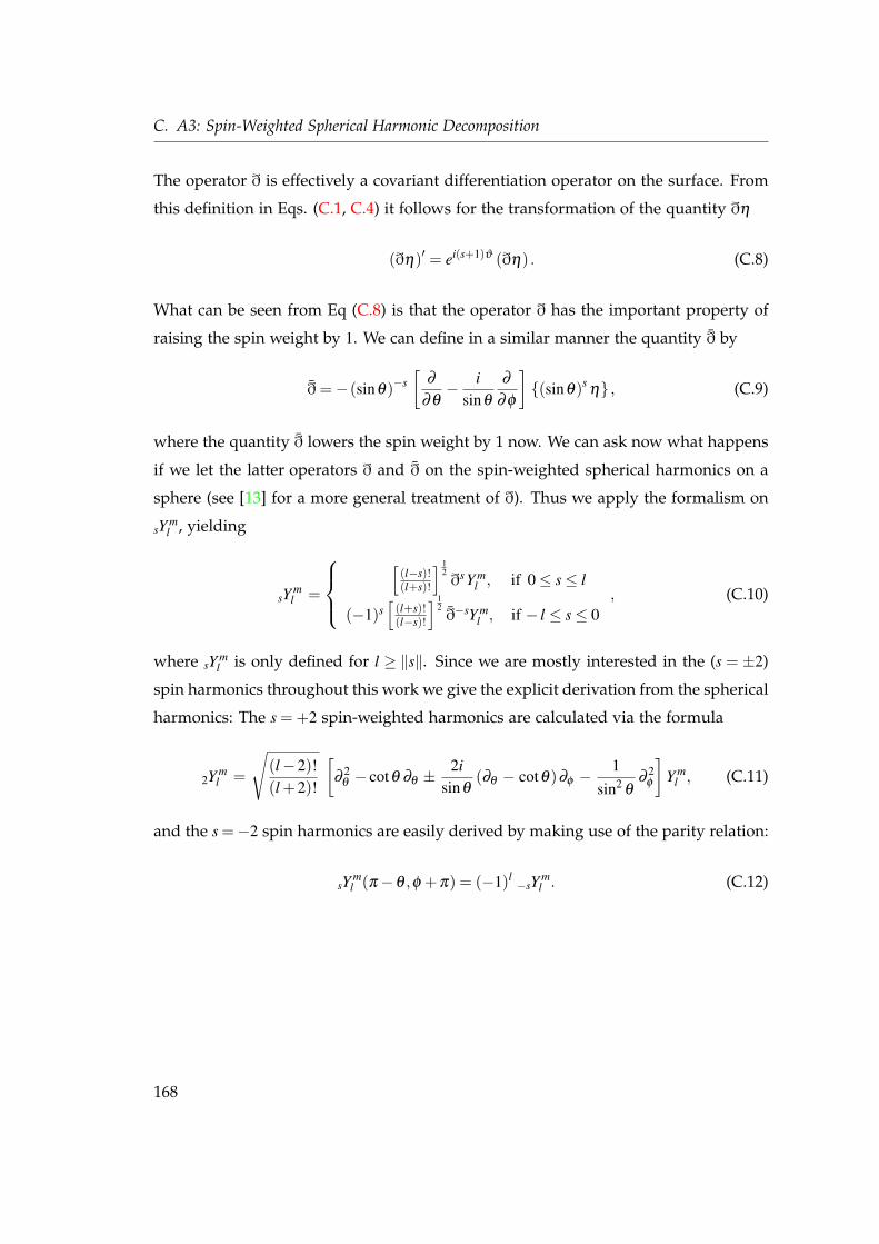
C. A3: Spin-Weighted Spherical Harmonic Decomposition
The operator ð is effectively a covariant differentiation operator on the surface. From
this definition in Eqs. (C.1, C.4) it follows for the transformation of the quantity ðη
(ðη)′ = ei(s+1)ϑ (ðη) . (C.8)
What can be seen from Eq (C.8) is that the operator ð has the important property of
raising the spin weight by 1. We can define in a similar manner the quantity ð by
ð =−(sinθ)−s[
∂
∂θ− i
sinθ
∂
∂φ
](sinθ)s
η , (C.9)
where the quantity ð lowers the spin weight by 1 now. We can ask now what happens
if we let the latter operators ð and ð on the spin-weighted spherical harmonics on a
sphere (see [13] for a more general treatment of ð). Thus we apply the formalism on
sY ml , yielding
sY ml =
[
(l−s)!(l+s)!
] 12 ðsY m
l , if 0≤ s≤ l
(−1)s[
(l+s)!(l−s)!
] 12 ð−sY m
l , if − l ≤ s≤ 0, (C.10)
where sY ml is only defined for l ≥ ‖s‖. Since we are mostly interested in the (s = ±2)
spin harmonics throughout this work we give the explicit derivation from the spherical
harmonics: The s = +2 spin-weighted harmonics are calculated via the formula
2Y ml =
√(l−2)!(l +2)!
[∂
2θ − cotθ ∂θ ±
2isinθ
(∂θ − cotθ)∂φ −1
sin2θ
∂2φ
]Y m
l , (C.11)
and the s =−2 spin harmonics are easily derived by making use of the parity relation:
sY ml (π−θ ,φ +π) = (−1)l
−sY ml . (C.12)
168
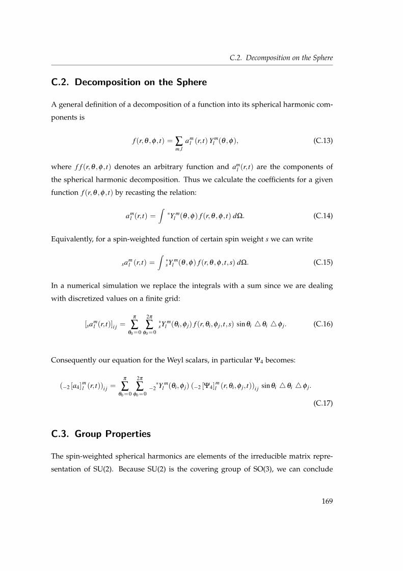
C.2. Decomposition on the Sphere
C.2. Decomposition on the Sphere
A general definition of a decomposition of a function into its spherical harmonic com-
ponents is
f (r,θ ,φ , t) = ∑m,l
aml (r, t) Y m
l (θ ,φ), (C.13)
where f f (r,θ ,φ , t) denotes an arbitrary function and aml (r, t) are the components of
the spherical harmonic decomposition. Thus we calculate the coefficients for a given
function f (r,θ ,φ , t) by recasting the relation:
aml (r, t) =
∫∗Y m
l (θ ,φ) f (r,θ ,φ , t) dΩ. (C.14)
Equivalently, for a spin-weighted function of certain spin weight s we can write
saml (r, t) =
∫∗sY m
l (θ ,φ) f (r,θ ,φ , t,s) dΩ. (C.15)
In a numerical simulation we replace the integrals with a sum since we are dealing
with discretized values on a finite grid:
[saml (r, t)]i j =
π
∑θ0 =0
2π
∑φ0 =0
∗sY m
l (θi,φ j) f (r,θi,φ j, t,s) sinθi 4θi 4φ j. (C.16)
Consequently our equation for the Weyl scalars, in particular Ψ4 becomes:
(−2 [a4]ml (r, t))i j =
π
∑θ0 =0
2π
∑φ0 =0
∗−2 Y m
l (θi,φ j) (−2 [Ψ4]ml (r,θi,φ j, t))i j sinθi 4θi 4φ j.
(C.17)
C.3. Group Properties
The spin-weighted spherical harmonics are elements of the irreducible matrix repre-
sentation of SU(2). Because SU(2) is the covering group of SO(3), we can conclude
169
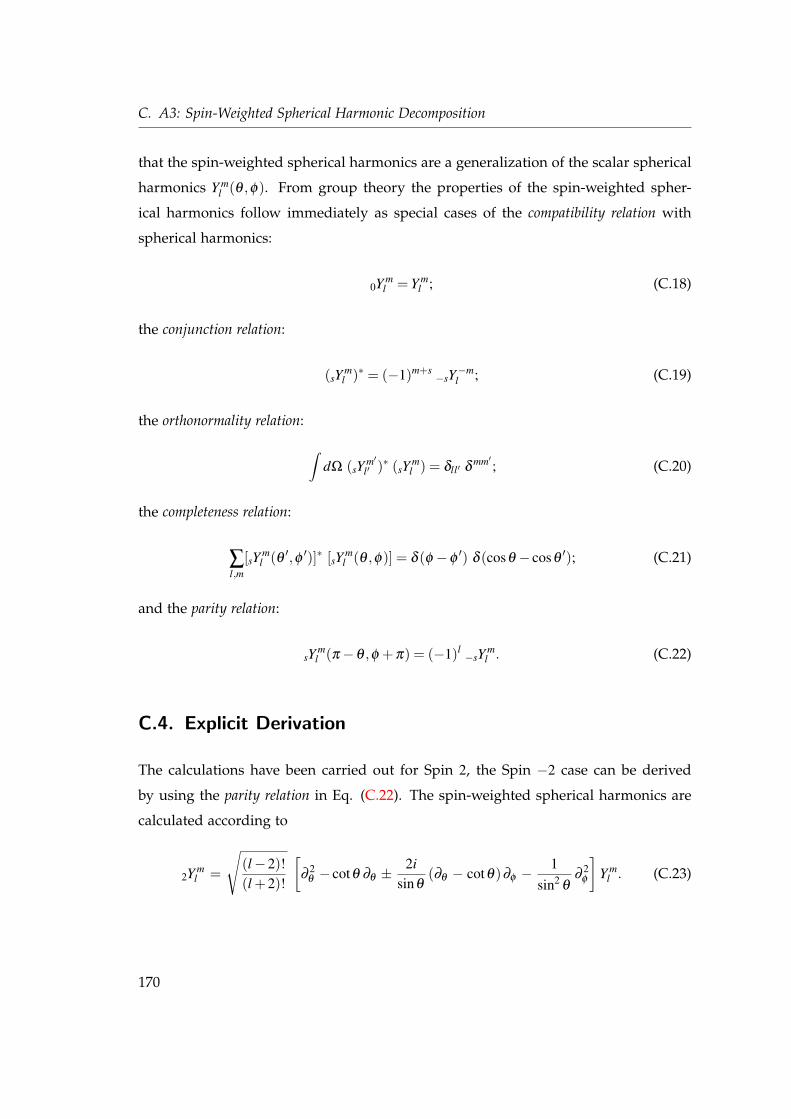
C. A3: Spin-Weighted Spherical Harmonic Decomposition
that the spin-weighted spherical harmonics are a generalization of the scalar spherical
harmonics Y ml (θ ,φ). From group theory the properties of the spin-weighted spher-
ical harmonics follow immediately as special cases of the compatibility relation with
spherical harmonics:
0Y ml = Y m
l ; (C.18)
the conjunction relation:
(sY ml )∗ = (−1)m+s
−sY−ml ; (C.19)
the orthonormality relation:
∫dΩ (sY m′
l′ )∗ (sY ml ) = δll′ δ
mm′ ; (C.20)
the completeness relation:
∑l,m
[sY ml (θ ′,φ ′)]∗ [sY m
l (θ ,φ)] = δ (φ −φ′) δ (cosθ − cosθ
′); (C.21)
and the parity relation:
sY ml (π−θ ,φ +π) = (−1)l
−sY ml . (C.22)
C.4. Explicit Derivation
The calculations have been carried out for Spin 2, the Spin −2 case can be derived
by using the parity relation in Eq. (C.22). The spin-weighted spherical harmonics are
calculated according to
2Y ml =
√(l−2)!(l +2)!
[∂
2θ − cotθ ∂θ ±
2isinθ
(∂θ − cotθ)∂φ −1
sin2θ
∂2φ
]Y m
l . (C.23)
170
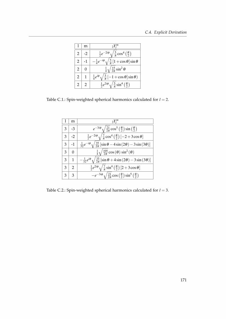
C.4. Explicit Derivation
l m 2Y ml
2 -2 12 e−2iφ
√5π
cos4(
θ
2
)2 -1 −1
4 e−iφ√
5π
[1+ cosθ ]sinθ
2 0 14
√152π
sin2θ
2 1 14 eiφ
√5π
[−1+ cosθ ]sinθ)
2 2 12 e2iφ
√5π
sin4 (θ
2
)Table C.1.: Spin-weighted spherical harmonics calculated for l = 2.
l m 2Y ml
3 -3 e−3iφ√
212π
cos5(
θ
2
)sin(
θ
2
)3 -2 1
2 e−2iφ√
7π
cos4(
θ
2
)[−2+3cosθ ]
3 -1 132 e−iφ
√352π
[sinθ −4sin(2θ)−3sin(3θ)]
3 0 14
√1052π
cos(θ) sin2 (θ)
3 1 − 132 eiφ
√352π
[sinθ +4sin(2θ)−3sin(3θ)]
3 2 12 e2iφ
√7π
sin4 (θ
2
)[2+3cosθ ]
3 3 −e−3iφ√
212π
cos(
θ
2
)sin5 (θ
2
)Table C.2.: Spin-weighted spherical harmonics calculated for l = 3.
171
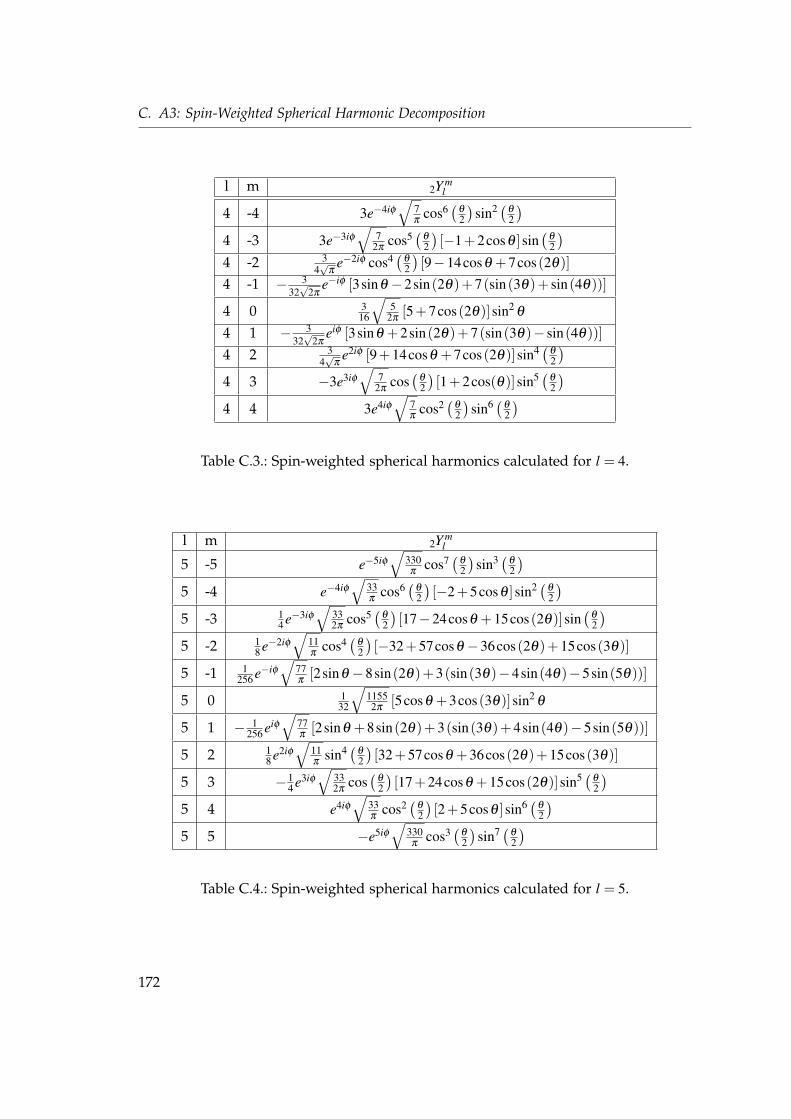
C. A3: Spin-Weighted Spherical Harmonic Decomposition
l m 2Y ml
4 -4 3e−4iφ√
7π
cos6(
θ
2
)sin2 (θ
2
)4 -3 3e−3iφ
√7
2πcos5
(θ
2
)[−1+2cosθ ]sin
(θ
2
)4 -2 3
4√
πe−2iφ cos4
(θ
2
)[9−14cosθ +7cos(2θ)]
4 -1 − 332√
2πe−iφ [3sinθ −2sin(2θ)+7(sin(3θ)+ sin(4θ))]
4 0 316
√5
2π[5+7cos(2θ)]sin2
θ
4 1 − 332√
2πeiφ [3sinθ +2sin(2θ)+7(sin(3θ)− sin(4θ))]
4 2 34√
πe2iφ [9+14cosθ +7cos(2θ)]sin4 (θ
2
)4 3 −3e3iφ
√7
2πcos(
θ
2
)[1+2cos(θ)]sin5 (θ
2
)4 4 3e4iφ
√7π
cos2(
θ
2
)sin6 (θ
2
)Table C.3.: Spin-weighted spherical harmonics calculated for l = 4.
l m 2Y ml
5 -5 e−5iφ√
330π
cos7(
θ
2
)sin3 (θ
2
)5 -4 e−4iφ
√33π
cos6(
θ
2
)[−2+5cosθ ]sin2 (θ
2
)5 -3 1
4 e−3iφ√
332π
cos5(
θ
2
)[17−24cosθ +15cos(2θ)]sin
(θ
2
)5 -2 1
8 e−2iφ√
11π
cos4(
θ
2
)[−32+57cosθ −36cos(2θ)+15cos(3θ)]
5 -1 1256 e−iφ
√77π
[2sinθ −8sin(2θ)+3(sin(3θ)−4sin(4θ)−5sin(5θ))]
5 0 132
√11552π
[5cosθ +3cos(3θ)]sin2θ
5 1 − 1256 eiφ
√77π
[2sinθ +8sin(2θ)+3(sin(3θ)+4sin(4θ)−5sin(5θ))]
5 2 18 e2iφ
√11π
sin4 (θ
2
)[32+57cosθ +36cos(2θ)+15cos(3θ)]
5 3 −14 e3iφ
√332π
cos(
θ
2
)[17+24cosθ +15cos(2θ)]sin5 (θ
2
)5 4 e4iφ
√33π
cos2(
θ
2
)[2+5cosθ ]sin6 (θ
2
)5 5 −e5iφ
√330π
cos3(
θ
2
)sin7 (θ
2
)Table C.4.: Spin-weighted spherical harmonics calculated for l = 5.
172
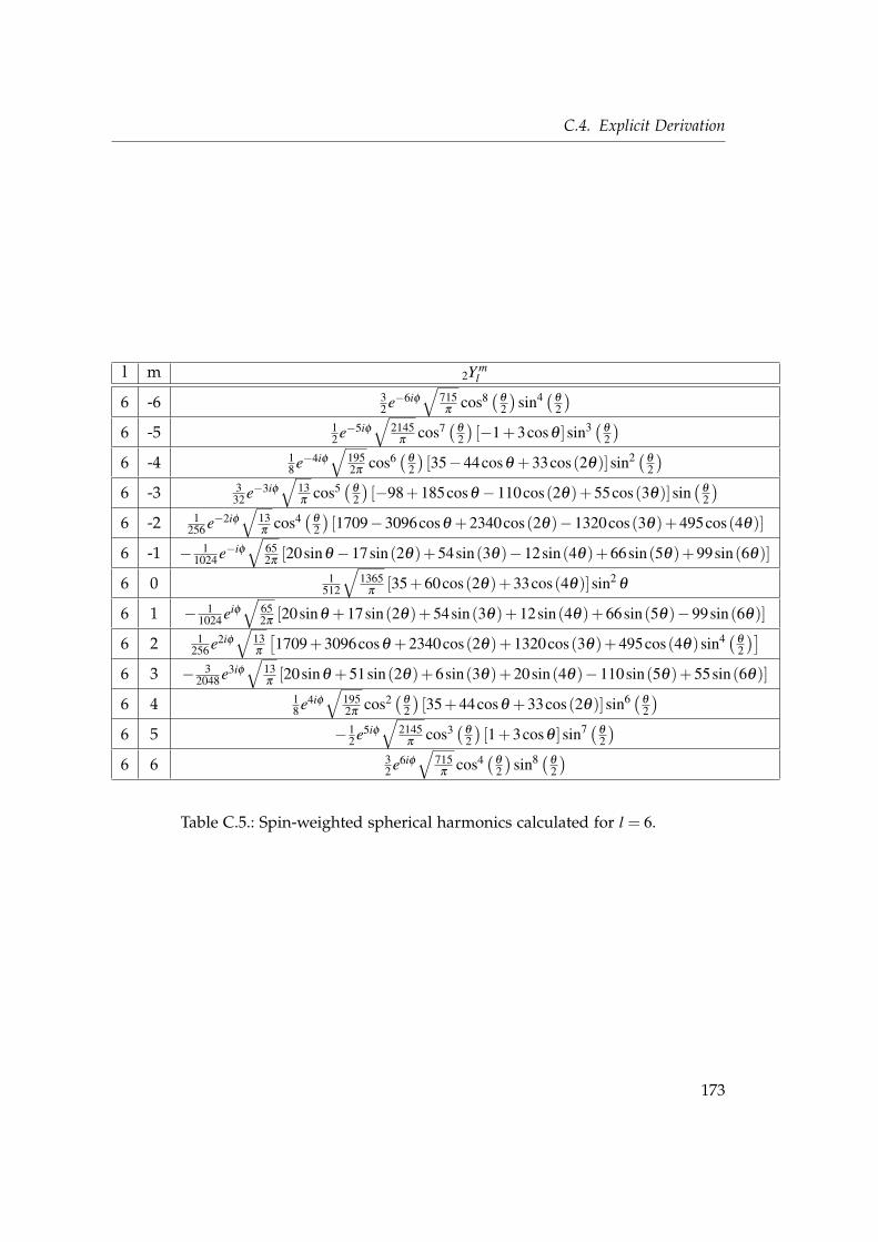
C.4. Explicit Derivation
l m 2Y ml
6 -6 32 e−6iφ
√715π
cos8(
θ
2
)sin4 (θ
2
)6 -5 1
2 e−5iφ√
2145π
cos7(
θ
2
)[−1+3cosθ ]sin3 (θ
2
)6 -4 1
8 e−4iφ√
1952π
cos6(
θ
2
)[35−44cosθ +33cos(2θ)]sin2 (θ
2
)6 -3 3
32 e−3iφ√
13π
cos5(
θ
2
)[−98+185cosθ −110cos(2θ)+55cos(3θ)]sin
(θ
2
)6 -2 1
256 e−2iφ√
13π
cos4(
θ
2
)[1709−3096cosθ +2340cos(2θ)−1320cos(3θ)+495cos(4θ)]
6 -1 − 11024 e−iφ
√652π
[20sinθ −17sin(2θ)+54sin(3θ)−12sin(4θ)+66sin(5θ)+99sin(6θ)]
6 0 1512
√1365
π[35+60cos(2θ)+33cos(4θ)]sin2
θ
6 1 − 11024 eiφ
√652π
[20sinθ +17sin(2θ)+54sin(3θ)+12sin(4θ)+66sin(5θ)−99sin(6θ)]
6 2 1256 e2iφ
√13π
[1709+3096cosθ +2340cos(2θ)+1320cos(3θ)+495cos(4θ)sin4 (θ
2
)]6 3 − 3
2048 e3iφ√
13π
[20sinθ +51sin(2θ)+6sin(3θ)+20sin(4θ)−110sin(5θ)+55sin(6θ)]
6 4 18 e4iφ
√1952π
cos2(
θ
2
)[35+44cosθ +33cos(2θ)]sin6 (θ
2
)6 5 −1
2 e5iφ√
2145π
cos3(
θ
2
)[1+3cosθ ]sin7 (θ
2
)6 6 3
2 e6iφ√
715π
cos4(
θ
2
)sin8 (θ
2
)Table C.5.: Spin-weighted spherical harmonics calculated for l = 6.
173
C. A3: Spin-Weighted Spherical Harmonic Decomposition
174
Bibliography
[1] A. Nerozzi, C. Beetle, M. Bruni, L. M. Burko, and D. Pollney. Towards a wave-
extraction method for numerical relativity. II. The quasi-Kinnersley frame. Phys.
Rev. D, 72(2):024014–+, July 2005.
[2] Greg Cook. Initial data for numerical relativity. Living Reviews in Relativity, 3(5),
2000.
[3] B. Abbott et al. Upper limits from the LIGO and TAMA detectors on the rate of
gravitational-wave bursts. Physical Review D, 72(12):122004–+, December 2005.
[4] B. Abbott et al. and LIGO Scientific Collaboration. First joint search for
gravitational-wave bursts in LIGO and GEO 600 data. Classical and Quantum
Gravity, 25(24):245008–+, December 2008.
[5] LIGO Scientific Collaboration. Search for Gravitational Waves from Low Mass
Compact Binary Coalescence in 186 Days of LIGO’s fifth Science Run. ArXiv
e-prints, May 2009.
[6] M. M. Jadhav and L. M. Burko. Black Hole Quasinormal Mode Spectroscopy
With LISA. The Astrophysical Journal, 698:562–566, June 2009.
[7] B. F. Schutz. Fundamental physics with LISA. Classical and Quantum Gravity,
26(9):094020–+, May 2009.
[8] R. A. Hulse and H. J. Taylor. Discovery of a Pulsar in a Close Binary System. In
Bulletin of the American Astronomical Society, volume 6 of Bulletin of the American
Astronomical Society, pages 453–+, September 1974.
175
Bibliography
[9] T. Regge and J. Wheeler. Stability of a Schwarzschild singularity. Phys. Rev.,
108(4):1063–1069, 1957.
[10] F. J. Zerilli. Effective potential for even-parity Regge-Wheeler gravitational per-
turbation equations. Phys. Rev. Lett., 24(13):737–738, 1970.
[11] E. Newman and R. Penrose. An approach to gravitational radiation by a method
of spin coefficients. J. Math. Phys., 3:566, 1962.
[12] E. Newman and T. Unti. Behavior of asymptotically flat empty spaces. J. Math.
Phys., 3:891, 1962.
[13] E. Newman and R. Penrose. Note on the bondi-metzner-sachs group. J. Math.
Phys., 7:863–870, 1966.
[14] Wiliam Press J.M. Bardeen. Radiation fields in the Schwarzschild background.
J. Math Phys, 14(1):7, 1973.
[15] S. A. Teukolsky. Perturbations of a rotating black hole. I. fundamental equations
for gravitational, electromagnetic, and neutrino-field perturbations. Astrophys.
J., 185:635–647, 1973.
[16] W. Kinnersley. Type d vacuum metrics. J. Math. Phys, 10:1195, 1969.
[17] R.K. Sachs. Proc. Roy. Soc. London, A270:103, 1962.
[18] R. Penrose. Asymptotic Properties of Fields and Space-Times. Physical Review
Letters, 10:66–68, January 1963.
[19] C. Beetle and L. Burko. Towards Wave Extraction in Numerical Relativity: Trans-
verse Frames. APS Meeting Abstracts, pages 10001–+, April 2005.
[20] C. Beetle, M. Bruni, L. M. Burko, and A. Nerozzi. Towards wave extraction
in numerical relativity: foundations and initial value formulation. 2004. gr-
qc/0407012.
[21] A. Nerozzi, C. Beetle, M. Bruni L.M. Burko, and D. Pollney. Towards wave ex-
traction in numerical relativity: the quasi-kinnersley frame. 2004. gr-qc/0407013.
176
Bibliography
[22] A. Nerozzi. Scalar functions for wave extraction in numerical relativity. Phys.
Rev. D, 75(10):104002–+, May 2007.
[23] M. Campanelli, B. Kelly, and C. O. Lousto. The Lazarus project. II. Spacelike
extraction with the quasi-Kinnersley tetrad. Phys. Rev. D, 73(6):064005–+, March
2006.
[24] J. W. York. Conformal ‘thin-sandwich’ data for the initial-value problem of gen-
eral relativity. Phys. Rev. Lett., 82:1350–1353, 1999.
[25] S. W. Hawking and G. F. R. Ellis. The large-scale structure of space-time. 1973.
[26] R. Penrose. Naked singularities. Ann. N.Y. Acad. Sci., 224:125, 1973.
[27] R. Arnowitt, S. Deser, and C. W. Misner. The dynamics of general relativity. In
L. Witten, editor, Gravitation: An Introduction to Current Research, pages 227–265.
John Wiley, New York, 1962.
[28] R. A. d’Inverno. In D. Bancel and M. Signore, editors, Problems of Collapse and
Numerical Relativity. Dordrecht, Reidel, 1984.
[29] K. Maeda, M. Sasaki, Takashi Nakamura, and S. Miyana. Prog. Theor. Phys.,
63:719, 1980.
[30] G. Yoneda and H. Shinkai. Advantages of modified ADM formulation: Con-
straint propagation analysis of the Baumgarte-Shapiro-Shibata-Nakamura sys-
tem. Phys. Rev. D, 66:124003, 2002.
[31] M. Shibata and Takashi Nakamura. Evolution of three-dimensional gravitational
waves: Harmonic slicing case. Phys. Rev. D, 52:5428, 1995.
[32] T. W. Baumgarte and S. L. Shapiro. Numerical integration of Einstein’s field
equations. Physical Review D, 59:024007, 1999.
[33] J. Baker, B. Brugmann, Manuela Campanelli, C. O. Lousto, and R. Taka-
hashi. Plunge waveforms from inspiralling binary black holes. Phys. Rev. Lett.,
87:121103, 2001.
177
Bibliography
[34] M. Alcubierre, W. Benger, B. Brugmann, G. Lanfermann, L. Nerger, E. Seidel,
and R. Takahashi. 3D Grazing Collision of Two Black Holes. Phys. Rev. Lett.,
87:271103, 2001.
[35] S. Brandt and B. Brugmann. A simple construction of initial data for multiple
black holes. Phys. Rev. Lett., 78(19):3606–3609, 1997.
[36] J. Weber. Gravitational-Wave-Detector Events. Physical Review Letters, 20:1307–
1308, June 1968.
[37] I. Ciufolini, V. Gorini, U. Moschella, and P. Fre, editors. Gravitational Waves,
2001.
[38] R. Takahashi, K. Arai, D. Tatsumi, M. Fukushima, T. Yamazaki, M.-K. Fujimoto,
K. Agatsuma, Y. Arase, N. Nakagawa, A. Takamori, K. Tsubono, R. DeSalvo,
A. Bertolini, S. Marka, V. Sannibale, and the TAMA Collaboration. Operational
status of TAMA300 with the seismic attenuation system (SAS). Classical and
Quantum Gravity, 25(11):114036–+, June 2008.
[39] B. Willke and the LIGO Scientific Collaboration. GEO600: status and plans.
Classical and Quantum Gravity, 24:389–+, October 2007.
[40] K. Kawabe and the LIGO Collaboration. Status of LIGO. Journal of Physics
Conference Series, 120(3):032003–+, July 2008.
[41] E. Tournefier and the VIRGO Collaboration. The status of virgo. Journal of
Physics Conference Series, 110(6):062025–+, May 2008.
[42] P. L. Bender. Proposed Laser Interferometer Space Antenna (LISA). In Bulletin
of the American Astronomical Society, volume 25 of Bulletin of the American Astro-
nomical Society, pages 1230–+, June 1993.
[43] S. Komossa. Observational evidence for supermassive black hole binaries. In
J. M. Centrella, editor, The Astrophysics of Gravitational Wave Sources, volume 686
of American Institute of Physics Conference Series, pages 161–174, October 2003.
178
Bibliography
[44] A. K. Sillanpaa. New Evidences for the OJ 287 Binary Black Hole Model. In
J. Paul, T. Montmerle, and E. Aubourg, editors, 19th Texas Symposium on Rela-
tivistic Astrophysics and Cosmology, December 1998.
[45] G. E. Romero, J.-H. Fan, and S. E. Nuza. The Binary Black Hole Scenario for the
BL Lacertae Object AO˜0235+16. Chinese Journal of Astronomy and Astrophysics,
3:513–525, December 2003.
[46] A. E. Broderick, A. Loeb, and R. Narayan. The Event Horizon of Sagittarius A*.
ArXiv e-prints, March 2009.
[47] J.-H. Woo, C. M. Urry, and R. P. et al. van der Marel. Black Hole Masses and Host
Galaxy Evolution of Radio-Loud Active Galactic Nuclei. Astrophysical Journal,
631:762–772, October 2005.
[48] D. S. Hudson, T. H. Reiprich, and T. E. et al. Clarke. X-ray detection of the proto
supermassive binary black hole at the centre of Abell 400. A& A, 453:433–446,
July 2006.
[49] H. Sudou. Detection of a supermassive black hole binary in an active galactic
nucleus. Astronomical Herald, 96:656–661, December 2003.
[50] A. Bachelot and A. Motet-Bachelot. Resonances of schwarzschild black holes. In
A. Donato and F. Oliveri, editors, Nonlinear Hyperbolic Problems: Theoretical and
Computational Aspects, volume 43 of Notes on Numerical Fluid Mechanics, Hap-
pauge, U.S.A., 1993. Informatica International.
[51] R.J. Gleiser, C.O. Nicasio, R.H. Price, and J. Pullin. Gravitational radiation from
schwarzschild black holes: the second-order perturbation formalism. Phys. Rep.,
325:41–81, 2000.
[52] S. Chandrasekhar. On the equations governing the perturbations of the
schwarzschild black hole. Proc. R. Soc. London, Ser. A, 343:289–298, 1975.
[53] V. Moncrief. Gravitational perturbations of spherically symmetric systems. i the
exterior problem. Ann. Phys. (N.Y.), 88:323–342, 1974.
179
Bibliography
[54] K.S. Thorne and A. Campolattaro. Non-radial pulsation of general-relativistic
stellar models. i. analytic analysis for `≥ 2. Astrophys. J., 149:591–611, 1967.
[55] Bernd Schmidt Kostas D. Kokkotas. Quasi-normal modes of stars and black
holes. Living Reviews in Relativity, 2(2), 1999.
[56] C. V. Vishveshwara. Stability of the Schwarzschild metric. Phys. Rev. D, 1:2870,
1970.
[57] B.F. Schutz and C.M. Will. Black hole normal modes: a semianalytic approach.
Astrophys. J. Lett., 291:L33–L36, 1985.
[58] H. Nakano and K. Ioka. Second-order quasinormal mode of the Schwarzschild
black hole. Phys. Rev. D, 76(8):084007–+, October 2007.
[59] P. Szekeres. The gravitational compass. J. Math. Phys, 6:1387–1391, 1965.
[60] C. Beetle, M. Bruni, L. M. Burko, and A. Nerozzi. Towards a wave-extraction
method for numerical relativity. I. Foundations and initial-value formulation.
Phys. Rev. D, 72(2):024013–+, July 2005.
[61] W. L. Bade and H. Jehle. An Introduction to Spinors. Reviews of Modern Physics,
25:714–728, July 1953.
[62] Roger Penrose and W. Rindler. Spinors and Spacetime, volume 1, 2. Cambridge
University Press, 1984, 1986.
[63] E. Kretschmann. Uber die prinzipielle Bestimmbarkeit der berechtigten
Bezugssysteme beliebiger Relativitatstheorien (II). Annalen der Physik, 353:943–
982, 1915.
[64] S. Chandrasekhar. The Mathematical Theory of Black Holes. Oxford University
Press, Oxford, England, 1983.
[65] H. Bondi, F.R. Sachs., M. G. J. van der Burg, and A. W. K. Metzner. Gravitational
waves in general relativity VII. waves from axi-symmetric isolated systems. Proc.
R. Soc., A269:21–52, 1962.
180
Bibliography
[66] R. Geroch. Energy Extraction. In D. J. Hegyi, editor, Sixth Texas Symposium on
Relativistic Astrophysics, volume 224 of New York Academy Sciences Annals, pages
108–+, 1973.
[67] E. T. Newman and K. P. Tod. Asymptotically Flat Space-Times. In General Rela-
tivity and Gravitation, pages 1–+, 1980.
[68] D. Pollney, J.E.F. Skea, and R.A. d’Inverno. Classifying geometries in general
relativity: I. standard forms for symmetric spinors. Class. Quantum Grav., 17:643–
663, 2000.
[69] G. D. Birkhoff and R. E. Langer. Relativity and modern physics. 1923.
[70] A. Nerozzi, M. Bruni, V. Re, and L. M. Burko. Towards a wave-extraction method
for numerical relativity. IV. Testing the quasi-Kinnersley method in the Bondi-
Sachs framework. Phys. Rev. D, 73(4):044020–+, February 2006.
[71] H. Stephani, D. Kramer, M. MacCallum, C. Hoenselaers, and E. Herlt. Exact
solutions of Einstein’s field equations. 2003.
[72] M. MacCallum D. Kramer, H. Stephani and E. Herlt. Exact Solutions of Einstein’s
Field Equations. Cambridge University Press, Cambridge, 1980.
[73] R.K. Sachs. Proc. Roy. Soc. London, A264:309, 1961.
[74] L. Lehner and O. M. Moreschi. Dealing with delicate issues in waveform calcu-
lations. Phys. Rev. D, 76(12):124040–+, December 2007.
[75] E. Gallo, L. Lehner, and O. M. Moreschi. Estimating total momentum at finite
distances. Phys. Rev. D, 78(8):084027–+, October 2008.
[76] E. Gallo, L. Lehner, and O. M. Moreschi. On computations of angular momen-
tum and its flux in numerical relativity. ArXiv e-prints, October 2008.
[77] D. S. Brill. On the positive definite mass of the Bondi-Weber-Wheeler time-
symmetric gravitational waves. Ann. Phys. (N. Y.), 7:466–483, 1959.
181
Bibliography
[78] S. G. Hahn and R. W. Lindquist. The two body problem in geometrodynamics.
Ann. Phys., 29:304–331, 1964.
[79] A. Cadez. Apparent horizons in the two-black-hole problem. Ann. Phys., 83:449–
457, 1974.
[80] K. Eppley. Evolution of time-symmetric gravitational waves: Initial data and
apparent horizons. Phys. Rev. D, 16(6):1609–1614, 1977.
[81] L. Smarr. Spacetimes generated by computers: Black holes with gravitational
radiation. Ann. N. Y. Acad. Sci., 302:569–604, 1977.
[82] K. Eppley. Pure gravitational waves. In L. Smarr, editor, Sources of Gravitational
Radiation, page 275. Cambridge University Press, Cambridge, England, 1979.
[83] A. Abrahams, D. Bernstein, D. Hobill, E. Seidel, and L. Smarr. Numerically
generated black hole spacetimes: Interaction with gravitational waves. Phys.
Rev. D, 45:3544–3558, 1992.
[84] D. Bernstein. A Numerical Study of the Black Hole Plus Brill Wave Spacetime. PhD
thesis, University of Illinois Urbana-Champaign, 1993.
[85] D. Bernstein, D. Hobill, E. Seidel, and L. Smarr. Initial data for the black hole
plus Brill wave spacetime. Phys. Rev. D, 50:3760, 1994.
[86] J. Karkowski and E. Malec. The general penrose inequality: lessons from nu-
merical evidence. ACTA PHYS.POLON.B, 36:59, 2005.
[87] M. Alcubierre, G. Allen, B. Brugmann, G. Lanfermann, E. Seidel, W.-M. Suen,
and M. Tobias. Gravitational collapse of gravitational waves in 3D numerical
relativity. Phys. Rev. D, 61:041501 (R), 2000.
[88] J. York. Initial data for collisions of black holes and other gravitational miscel-
lany. In C. Evans, L. Finn, and D. Hobill, editors, Frontiers in Numerical Relativity,
pages 89–109. Cambridge University Press, Cambridge, England, 1989.
182
Bibliography
[89] S. Dain. A variational principle for stationary, axisymmetric solutions of ein-
stein’s equations. 2005. gr-qc/0508061.
[90] D. Holz, W. Miller, M. Wakano, and J. Wheeler. In B. Hu and T. Jacobson, editors,
Directions in General Relativity: Proceedings of the 1993 International Symposium,
Maryland; Papers in honor of Dieter Brill, Cambridge, England, 1993. Cambridge
University Press.
[91] A. Einstein and N. Rosen. The particle problem in the general theory of relativ-
ity. Phys. Rev. D, 48:73, 1935.
[92] C. Misner. Wormhole initial conditions. Phys. Rev. D, 118(4):1110–1111, 1960.
[93] D. Brill and R. Lindquist. Interaction energy in geometrostatics. Phys. Rev.,
131:471–476, 1963.
[94] B. Brugmann, J. A. Gonzalez, M. Hannam, S. Husa, U. Sperhake, and W. Tichy.
Calibration of moving puncture simulations. Phys. Rev. D, 77(2):024027–+, Jan-
uary 2008.
[95] D. Bernstein, D. Hobill, E. Seidel, L. Smarr, and J. Towns. Numerically generated
axisymmetric black hole spacetimes: Numerical methods and code tests. Phys.
Rev. D, 50(8):5000–5024, 1994.
[96] D. Bernstein and K. P. Tod. Penrose’s quasi-local-mass in a numerically com-
puted space-time. Phys. Rev. D, 49(6):2808–2819, 1994.
[97] O. Elbracht, A. Nerozzi, and R. Matzner. Wave extraction in numerical evolu-
tions of distorted black holes. OCLC’s Experimental Thesis Catalog (United States),
2005.
[98] W. H. Press and S. A. Teukolsky. Perturbations of a Rotating Black Hole. II.
Dynamical Stability of the Kerr Metric. Astrophys. J., 185:649–674, October 1973.
[99] O. M. Moreschi. Angular momentum of future null infinity. In Fourth Marcel
Grossmann Meeting on General Relativity, pages 1687–1694, 1986.
183
Bibliography
[100] A. Rizzi. Angular Momentum in General Relativity: A New Definition. Physical
Review Letters, 81:1150–1153, August 1998.
[101] M. Streubel. “Conserved” quantities for isolated gravitational systems. General
Relativity and Gravitation, 9:551–561, June 1978.
[102] T. Dray and M. Streubel. Angular momentum at null infinity. Classical and
Quantum Gravity, 1:15–26, January 1984.
[103] B. D. Bramson. Relativistic Angular Momentum for Asymptotically Flat
Einstein-Maxwell Manifolds. Royal Society of London Proceedings Series A, 341:463–
490, January 1975.
[104] J. Winicour. Angular momentum in general relativity. In General relativity and
gravitation, Vol. 2, p. 71 - 96, volume 2, pages 71–96, 1980.
[105] C. R. Prior. Angular momentum in general relativity. I. Definition and asymp-
totic behaviour. Royal Society of London Proceedings Series A, 354:379–405, 1977.
[106] L. A. Tamburino and J. H. Winicour. Gravitational Fields in Finite and Confor-
mal Bondi Frames. Physical Review, 150:1039–1053, October 1966.
[107] J. Winicour. Some Total Invariants of Asymptotically Flat Space-Times. Journal
of Mathematical Physics, 9:861–867, June 1968.
[108] L. Smarr. The Structure of General Relativity with a Numerical Illustration: The
Collision of Two Black Holes. PhD thesis, University of Texas, Austin, Austin,
Texas, 1975.
[109] J. N. Goldberg, A. J. MacFarlane, E. T. Newman, F. Rohrlich, and E. C. G. Sudar-
shan. J. Math. Phys., 8:2155, 1967.
184

185

186
Curriculum Vitae
Oliver ElbrachtGegenbaurstraße 8b
97074 Wurzburg
E-Mail [email protected]
Geburtsdatum, -ort 20. Juli 1982, Warendorf, NRW
Nationalitat Deutsch
Ausbildung1988 - 1992 Grundschule Hamm, NRW
1992 - 2001 Freiherr-vom-Stein-Gymnasium Hamm, NRW
Juni 2001 Abitur; Gesamtnote 1,8
10/2001 - 8/2004 Studium der Physik an der Universitat Wurzburg
Oktober 2003 Vordiplom; Durchschnittsnote 1,5
8/2004 - 12/2005 Studium der Physik an der University of Texas at Austin, USA
Dezember 2005 Abschluss Master of Arts; Note A / GPA 3.83
seit Oktober 2006 Dissertation, Julius-Maximilians-Universitat Wurzburg
Stipendien & Jobsseit Januar 2006 Wissenschaftlicher Mitarbeiter an der Universitat Wurzburg
8/2004 - 8/2005 Stipendium des Deutschen Akademischen Austausch Dienstes (DAAD)
seit 6/2007 Stipendiat des Elitenetzwerk Bayern (ENB)
seit 8/2007 Mitglied des Graduiertenkollegs 1147/1 der Universitat Wurzburg
187

188
Acknowledgements
I wish to thank...
...Karl Mannheim for all the financial and personal support he has provided to make
this work possible. His exceptional knowledge of physics and the inspiring discus-
sions with him gave me a unique opportunity to prepare this work.
...Thomas Trefzger for his immediate readiness to write the additional report on this
dissertation.
...Felix Spanier who greatly helped me with administrational and financial issues.
...Andrea Nerozzi for his guidance planning and preparing this thesis.
...Thomas Burkart and Michael Ruger for their friendship, the professional teamwork
and the great insanity at the office and outside the university.
...The makers of Bomberclone.
...Katharina Eisler for all her support and patience.
Special thanks go to my parents, who have always done everything they could to
support me.
Without words, without writing and without books
there would be no history,
there could be no concept of humanity.
(Hermann Hesse)
189