Automatic Identification of Ice Layers in Radar Echograms

David Crandall, Jerome Mitchell, Geoffrey C. FoxSchool of Informatics and ComputingIndiana University, USA

John D. PadenCenter for Remote Sensing of Ice SheetsUniversity of Kansas, USA

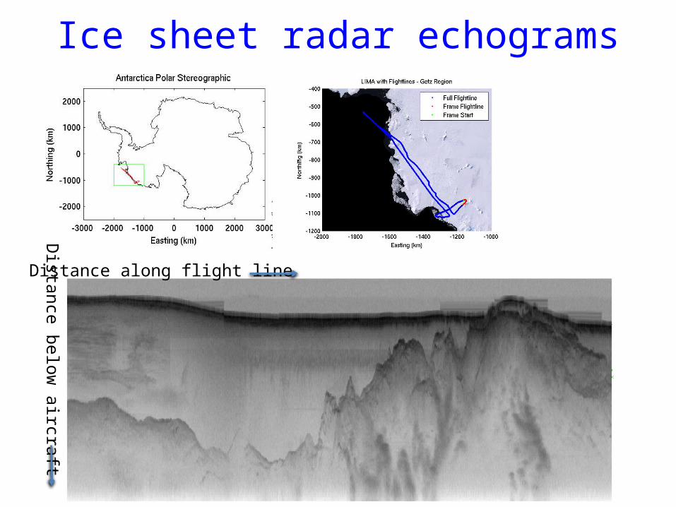
Ice sheet radar echograms

Distance along flight lineDistance below

aircraft

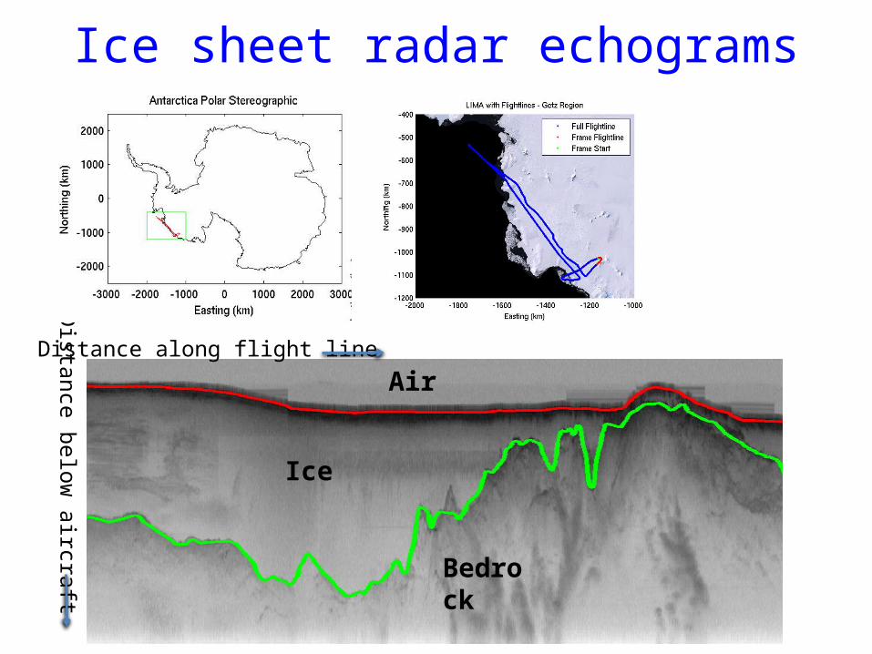
Ice sheet radar echograms

Bedrock

Ice

Distance along flight lineDistance below

aircraft

Air

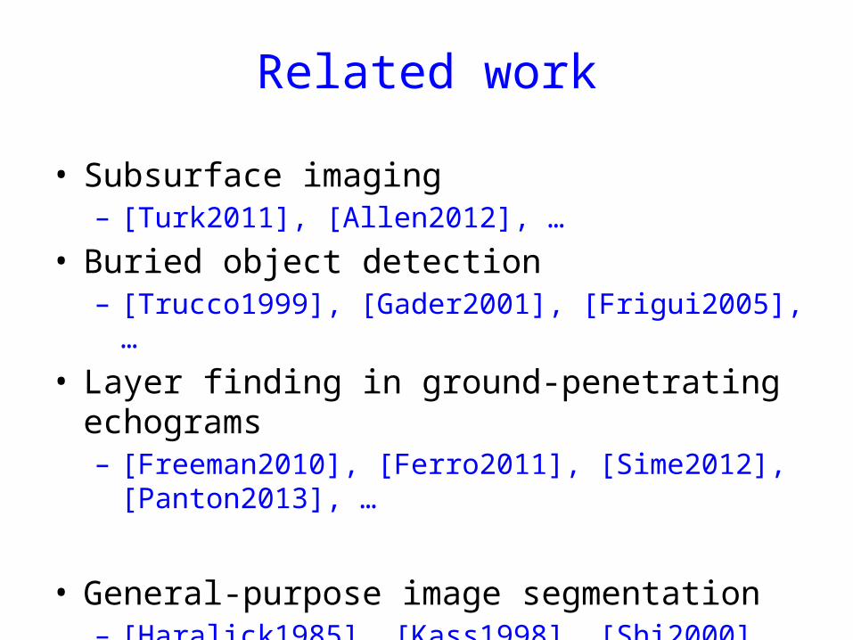
Related work

• Subsurface imaging – [Turk2011], [Allen2012], …

• Buried object detection – [Trucco1999], [Gader2001], [Frigui2005], …

• Layer finding in ground-penetrating echograms – [Freeman2010], [Ferro2011], [Sime2012], [Panton2013], …

• General-purpose image segmentation– [Haralick1985], [Kass1998], [Shi2000], [Felzenszwalb2004], …

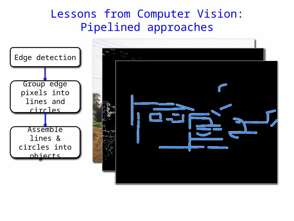
Lessons from Computer Vision:Pipelined approaches

Edge detection

Group edge pixels into lines and circles

Assemble lines & circles into objects

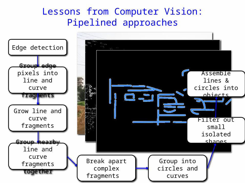
Lessons from Computer Vision:Pipelined approaches

Edge detection

Group edge pixels into line and curve

fragments

Grow line and curve fragments

Group nearby line and curve

fragments together Break apart complex fragments

Group into circles and curves

Filter out small isolated shapes

Assemble lines & circles into objects

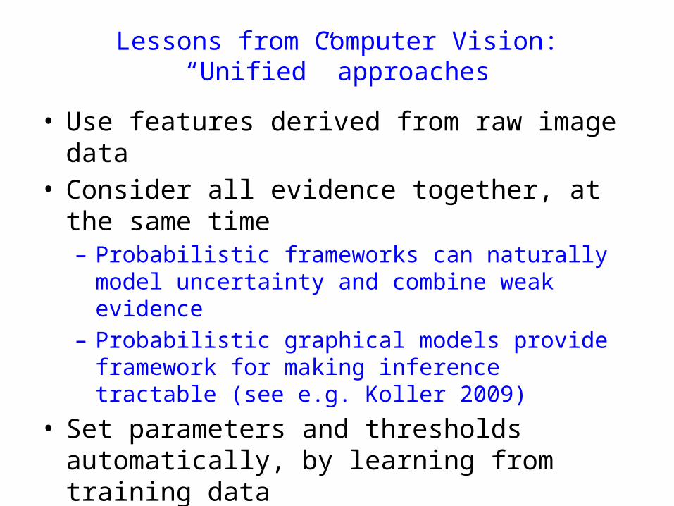
Lessons from Computer Vision:“Unified” approaches

• Use features derived from raw image data• Consider all evidence together, at the same time– Probabilistic frameworks can naturally model uncertainty

and combine weak evidence– Probabilistic graphical models provide framework for

making inference tractable (see e.g. Koller 2009)

• Set parameters and thresholds automatically, by learning from training data

Tiered segmentation• Layer-finding is a tiered segmentation

problem [Felzenszwalb2010]– Label each pixel with one of [1, K+1],

under the constraint that if y < y’, label of (x, y) ≤ label of (x, y’)

• Equivalently, find K boundaries in each column– Let denote the row indices of the K region

boundaries in column i– Goal is to find labeling of whole image,

Li

li1

li2

li3

1

2

3

4

2

Crandall, Fox, Paden, International Conference on Pattern Recognition (ICPR), 2012.

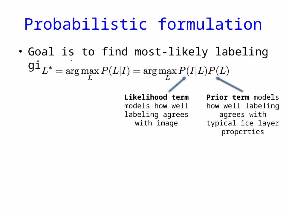
Probabilistic formulation

• Goal is to find most-likely labeling given image I,

Likelihood term models how well labeling agrees with image

Prior term models how well labeling agrees with

typical ice layer properties

Prior term

• Prior encourages smooth, non-crossing boundaries

Zero-mean Gaussian penalizes discontinuities in layer

boundaries across columns

Repulsive term prevents boundary crossings; is 0 if

and uniform otherwise

li1

li2

li3

li+11

li+12

li+13

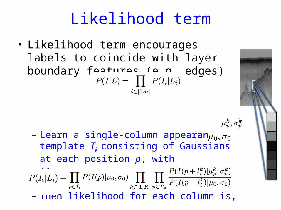
Likelihood term

• Likelihood term encourages labels to coincide with layer boundary features (e.g. edges)

– Learn a single-column appearance template Tk

consisting of Gaussians at each position p, with– Also learn a simple background model, with– Then likelihood for each column is,

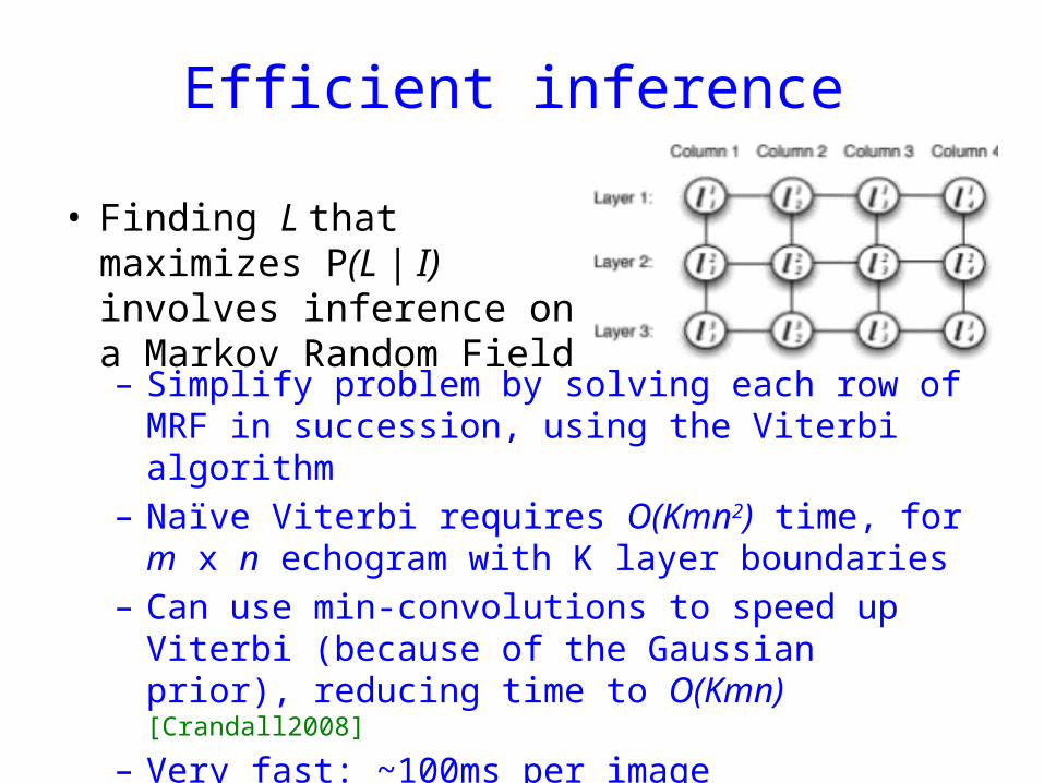
Efficient inference

• Finding L that maximizes P(L | I) involves inference on a Markov Random Field

– Simplify problem by solving each row of MRF in succession, using the Viterbi algorithm

– Naïve Viterbi requires O(Kmn2) time, for m x n echogram with K layer boundaries

– Can use min-convolutions to speed up Viterbi (because of the Gaussian prior), reducing time to O(Kmn) [Crandall2008]

– Very fast: ~100ms per image

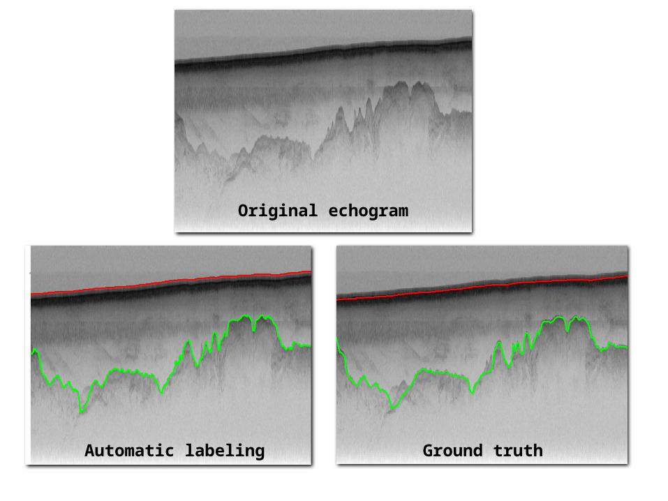
Experimental results

• Tested finding surface and bedrock layer boundaries, with 827 echograms from Antarctica– From Multichannel Coherent Radar Depth Sounder system

in 2009 NASA Operation Ice Bridge [Allen12]

– About 24,810 km of flight data– Split into equal-size training and test datasets

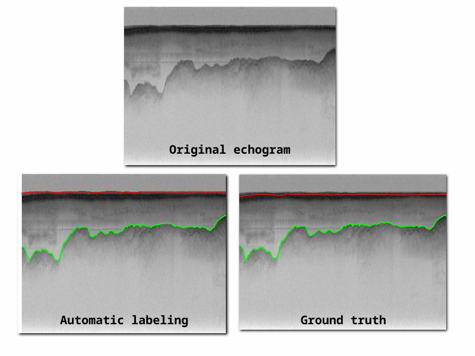
Original echogram

Automatic labeling Ground truth

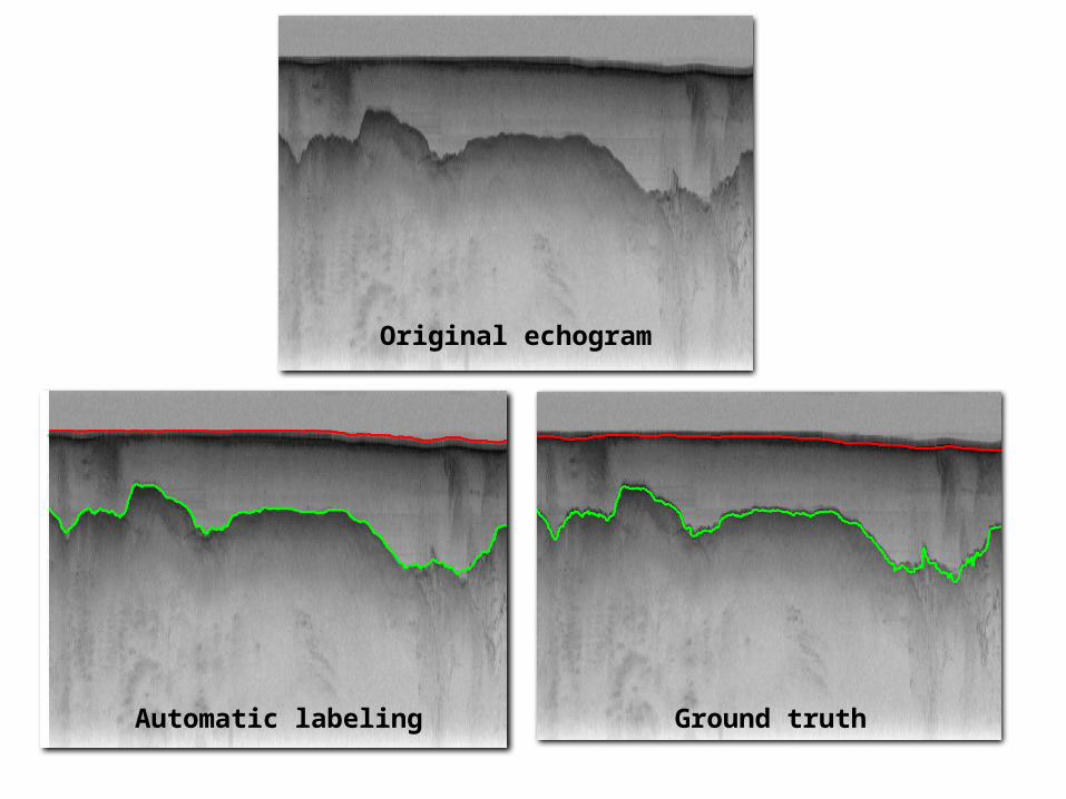
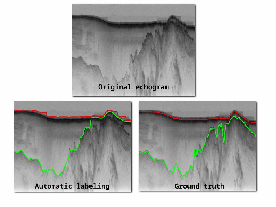
Original echogram

Automatic labeling Ground truth

Original echogram

Automatic labeling Ground truth

Original echogram

Automatic labeling Ground truth

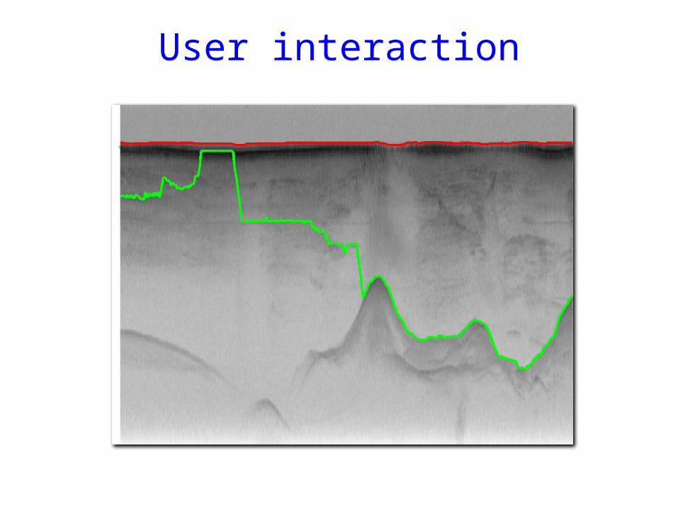
User interaction

User interaction

**

User interaction

**Modify P(L) such that this label has probability 1

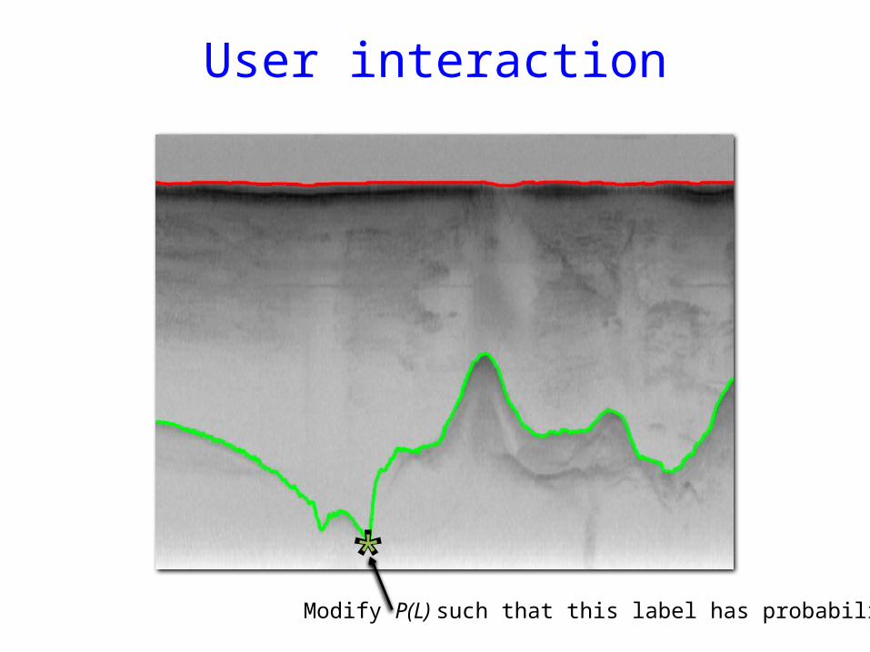
User interaction

**Modify P(L) such that this label has probability 1

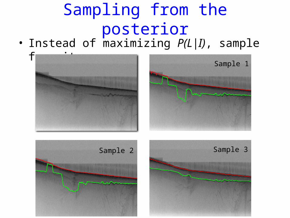
Sampling from the posterior• Instead of maximizing P(L|I), sample from it

Sample 1

Sample 2 Sample 3

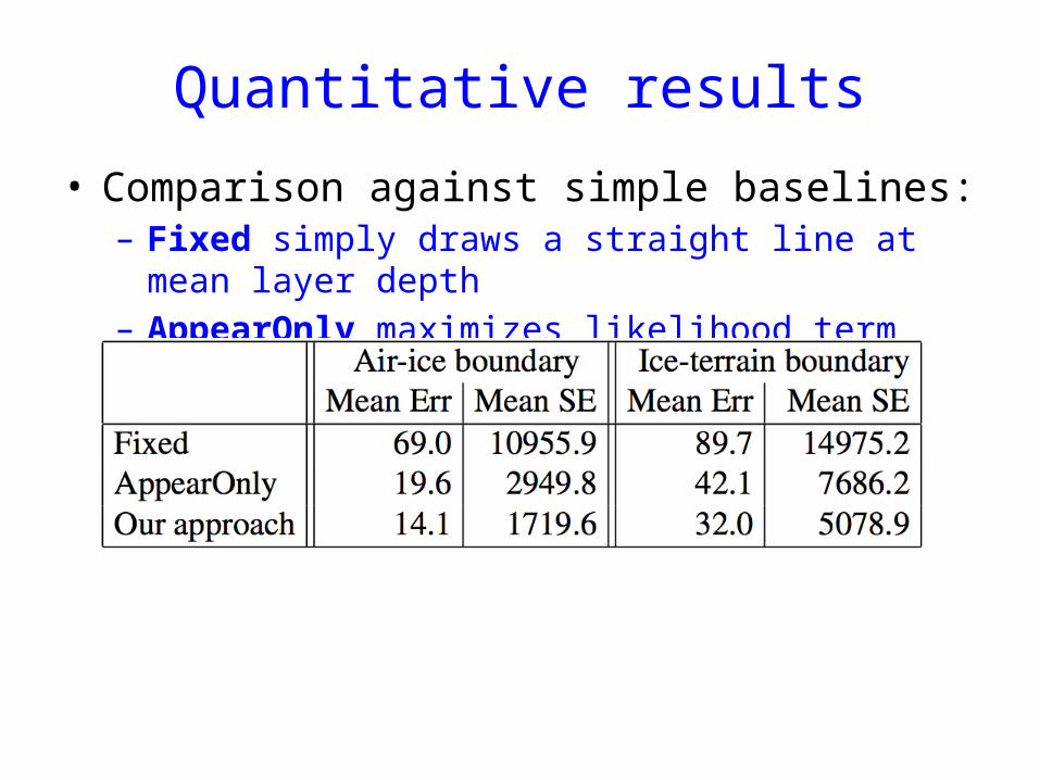
Quantitative results

• Comparison against simple baselines:– Fixed simply draws a straight line at mean layer depth– AppearOnly maximizes likelihood term only

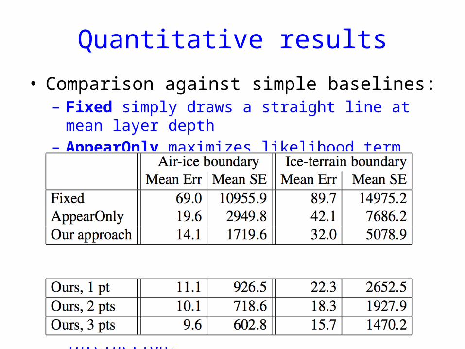
Quantitative results

• Comparison against simple baselines:– Fixed simply draws a straight line at mean layer depth– AppearOnly maximizes likelihood term only

– Further improvement with human interaction:

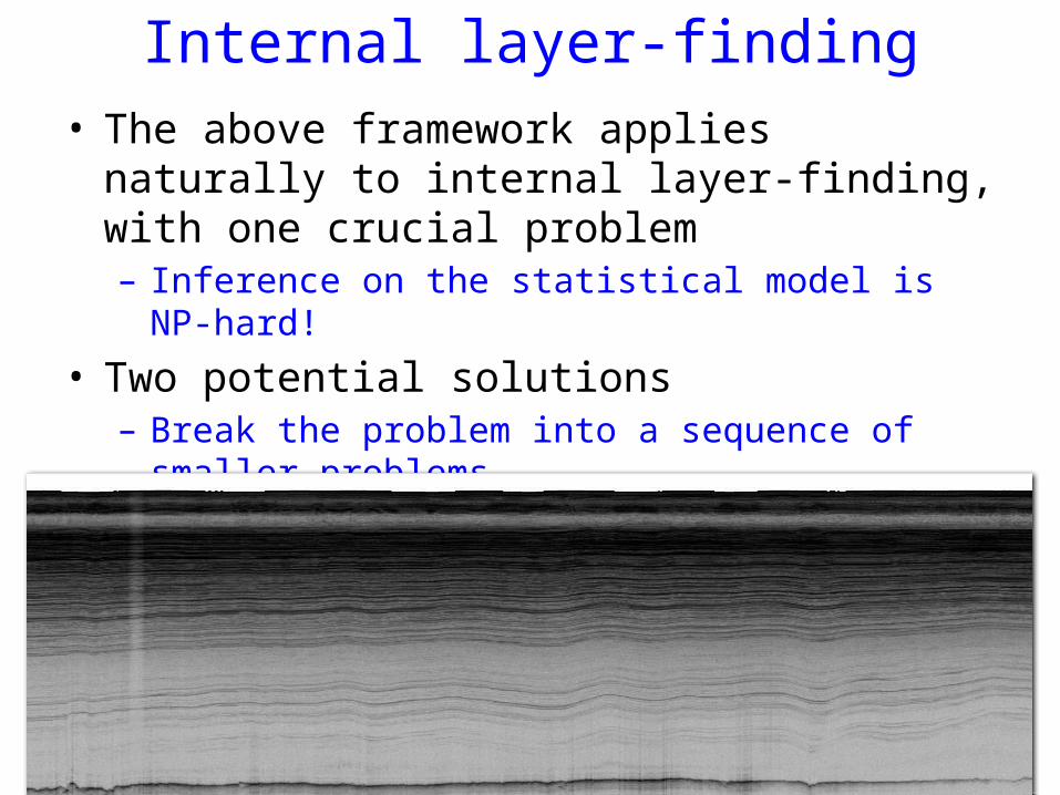
Internal layer-finding• The above framework applies naturally to internal

layer-finding, with one crucial problem– Inference on the statistical model is NP-hard!

• Two potential solutions– Break the problem into a sequence of smaller problems– Use an approximation algorithm to do the optimization;

we use loopy belief propagation

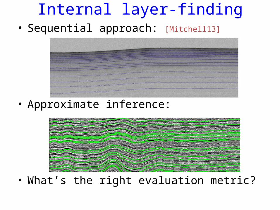
Internal layer-finding• Sequential approach: [Mitchell13]

• Approximate inference:

• What’s the right evaluation metric?

Summary and Future work• We present a probabilistic technique for ice sheet

layer-finding from radar echograms– Inference is robust to noise and very fast– Parameters can be learned from training data– Easily include evidence from external sources

• Ongoing and future work– How to evaluate quality of labeling?– Explicitly modeling sources of noise in radar images– Full 3d inference: Solving for all layers in 3d, using data

from all flight tracks as well as cores, etc.

More information available at:http://vision.soic.indiana.edu/icelayers/

This work was supported in part by:

Thanks!