automatic classification of ground-penetrating-radar
TRANSCRIPT
University of Wollongong University of Wollongong
Research Online Research Online
Faculty of Informatics - Papers (Archive) Faculty of Engineering and Information Sciences
2011
Automatic Classification of Ground-Penetrating-Radar Signals for Railway-Automatic Classification of Ground-Penetrating-Radar Signals for Railway-
Ballast Assessment Ballast Assessment
Wenbin Shao University of Wollongong, [email protected]
Abdesselam Bouzerdoum University of Wollongong, [email protected]
Son Lam Phung University of Wollongong, [email protected]
Lijun Su University of Wollongong - Dubai Campus, [email protected]
Buddhima Indraratna University of Wollongong, [email protected]
See next page for additional authors
Follow this and additional works at: https://ro.uow.edu.au/infopapers
Part of the Physical Sciences and Mathematics Commons
Recommended Citation Recommended Citation Shao, Wenbin; Bouzerdoum, Abdesselam; Phung, Son Lam; Su, Lijun; Indraratna, Buddhima; and Rujikiatkamjorn, Cholachat: Automatic Classification of Ground-Penetrating-Radar Signals for Railway-Ballast Assessment, IEEE Transactions on Geoscience and Remote Sensing: 49(10) 2011, 3961-3972. https://ro.uow.edu.au/infopapers/1247
Research Online is the open access institutional repository for the University of Wollongong. For further information contact the UOW Library: [email protected]

Automatic Classification of Ground-Penetrating-Radar Signals for Railway-Ballast Automatic Classification of Ground-Penetrating-Radar Signals for Railway-Ballast Assessment Assessment
Abstract Abstract The ground-penetrating radar (GPR) has been widely used in many applications. However, the processing and interpretation of the acquired signals remain challenging tasks since an experienced user is required to manage the entire operation. In this paper, we present an automatic classification system to assess railway-ballast conditions. It is based on the extraction of magnitude spectra at salient frequencies and their classification using support vector machines. The system is evaluated on real-world railway GPR data. The experimental results show that the proposed method efficiently represents the GPR signal using a small number of coefficients and achieves a high classification rate when distinguishing GPR signals reflected by ballasts of different conditions.
Keywords Keywords Ground-penetrating radar (GPR) processing, railway-ballast assessment, support vector machine (SVM)
Disciplines Disciplines Physical Sciences and Mathematics
Publication Details Publication Details W. Shao, A. Bouzerdoum, S. L. Phung et al., “Automatic Classification of Ground-Penetrating-Radar Signals for Railway-Ballast Assessment,” IEEE Transactions on Geoscience and Remote Sensing, vol. 49, no. 10, 2011, pp. 3961-3972. Copyright IEEE 2011. Original item available here
Authors Authors Wenbin Shao, Abdesselam Bouzerdoum, Son Lam Phung, Lijun Su, Buddhima Indraratna, and Cholachat Rujikiatkamjorn
This journal article is available at Research Online: https://ro.uow.edu.au/infopapers/1247

IEEE TRANSACTIONS ON GEOSCIENCE & REMOTE SENSING 1
Automatic classification of ground penetrating radar
signals for railway ballast assessmentWenbin Shao, Abdesselam Bouzerdoum, Senior Member, IEEE, Son Lam Phung, Member, IEEE,
Lijun Su, Buddhima Indraratna, and Cholachat Rujikiatkamjorn
Abstract—Ground penetrating radar has been widely usedin many applications. However, the processing and interpreta-tion of the acquired signals remain challenging tasks since anexperienced user is required to manage the entire operation.In this paper, we present an automatic classification system toassess railway ballast conditions. It is based on the extraction ofmagnitude spectra at salient frequencies and their classificationusing support vector machines. The system is evaluated onreal-world railway GPR data. The experimental results showthat the proposed method efficiently represents the GPR signalusing a small number of coefficients, and achieves a highclassification rate when distinguishing ground penetrating radarsignals reflected by ballast of different conditions.
Index Terms—Railway ballast assessment, ground penetratingradar processing, support vector machine.
I. INTRODUCTION
GROUND penetrating radar (GPR), sometimes called sub-
surface radar, ground probing radar, georadar or earth
sounding radar, exploits electromagnetic fields to probe lossy
dielectric materials [1, 2, 3, 4]. It can non-destructively detect
buried objects beneath the shallow earth surface (less than
50 m) or in a visually impenetrable structure, such as walls
and concrete floors. GPR has attracted considerable interest
in many areas, such as archaeology [5], road construction [6],
glacier and ice sheet investigation [7], and mineral exploration
and resource evaluation [8].
As a cost-effective and environment-friendly means of trans-
portation, railway plays an important role in daily life. A
railway structure typically consists of steel rails, fastening
system, sleepers, ballast, subballast and subgrade [9]. The
transverse section of a railway is given in Fig. 1. The ballast
is an essential component for proper railway functioning.
To ensure safety, regular inspection of rail tracks must be
conducted. Traditionally, track investigation involves drilling
to collect ballast samples from the railway sites. The ballast
samples are then sent to a laboratory for assessment, which
involves fouling index measurement. Finally, maintenance
actions are determined based on the evaluation results. The
entire procedure is labor-intensive and time-consuming. Thus,
the rail industry is searching for new and more cost-effective
approaches. As a non-destructive detection tool, ground pen-
etrating radar has attracted great interest in railway ballast
evaluation in recent years [10].
Despite its commercial success, GPR still faces various
fundamental problems. Specifically, processing and interpret-
ing radar profiles are still challenging tasks [12, 13]. In
addition to traditional GPR processing techniques, such as
RailFastening system
Subgrade
Fouled ballast or subballast
Mostly clean ballast
Clean ballastSleeper
Ballast
Placed soil (fill)
Natural ground (formation)
Fig. 1. Railway structure [9, 11].
dewow and filtering, researchers have employed various signal
processing techniques to aid the GPR signal analysis and
interpretation [2, 13, 14]. For example, Al-Qadi et al. proposed
a time-frequency approach to evaluate GPR data for railway
ballast assessment [9]. Their approach utilizes the short-time
Fourier transform (STFT). Sinha et al. presented a new method
for time-frequency map computation for non-stationary sig-
nals [15]. Their approach utilizes the continuous wavelet
transform (CWT). Experiments on seismic data show that the
CWT approach can be used to detect frequency shadows and
subtle stratigraphic features. Fujimoto and Nonami suggested a
mine detection algorithm based on statistical features, such as
Student’s t-distribution and chi-square distribution [16]. Their
algorithm was shown to improve the probability of detection
and decrease the probability of false alarm. Zoubir et al.
compared a number of landmine detection techniques, such
as Kalman filtering, background subtraction, matched filter
de-convolution, wavelet packet decomposition and trimmed
average power [14]. They evaluated the techniques using
receiver operating characteristic curves and computation time.
The Kalman filtering approach was found to outperform other
methods on detection rate, but it has the highest computational
cost. The aforementioned studies mainly focus on improving
visualization and clarity of GPR signals, and human inter-
vention is still required to interpret the processed signals,
which may introduce subjectivity and user-dependency into
data analysis.
In a GPR survey, because particular resonance frequencies
arise in wave propagation, reflected waves from different
buried objects or paths present different electromagnetic char-
acteristics. Hence, it is possible to classify the buried objects
or underground materials by analyzing the frequency spectra
of the received GPR signals. Motivated by this observation,
we propose a GPR signal classification system based on
magnitude spectrum and support vector machines (SVMs) for
ballast fouling assessment. The proposed system is designed
so that no human intervention is required. It can automatically
IEEE TRANSACTIONS ON GEOSCIENCE & REMOTE SENSING 2
extract and select features from GPR railway signals, and
classify the GPR traces.
The remainder of the paper is organized as follows. In
Section II, the proposed classification system is introduced. In
Section III, the experimental methods and system implemen-
tation are explained. The experimental results are presented
in Section IV, followed by some concluding remarks in
Section V.
II. PROPOSED APPROACH
In this section, we first give an overview of the GPR system,
and then present the proposed approach for ballast fouling
classification.
A. GPR system overview
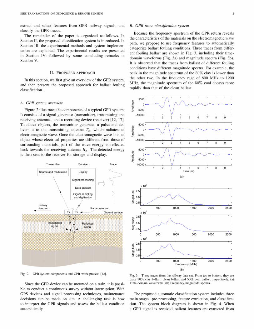
Figure 2 illustrates the components of a typical GPR system.
It consists of a signal generator (transmitter), transmitting and
receiving antennas, and a recording device (receiver) [12, 17].
To detect objects, the transmitter generates a pulse and de-
livers it to the transmitting antenna Tx, which radiates an
electromagnetic wave. Once the electromagnetic wave hits an
object whose electrical properties are different from those of
surrounding materials, part of the wave energy is reflected
back towards the receiving antenna Rx. The detected energy
is then sent to the receiver for storage and display.
Tx Rx
Survey
direction
Transmitted
signalReflected
signal
Transmitter
Source and modulation
Receiver
Radar antenna
Trace
Signal sampling
and digitisation
Data storage
Signal processing
Display
Ground surface
Fig. 2. GPR system components and GPR work process [12].
Since the GPR device can be mounted on a train, it is possi-
ble to conduct a continuous survey without interruption. With
GPS devices and signal processing techniques, maintenance
decisions can be made on site. A challenging task is how
to interpret the GPR signals and assess the ballast condition
automatically.
B. GPR trace classification system
Because the frequency spectrum of the GPR return reveals
the characteristics of the materials on the electromagnetic wave
path, we propose to use frequency features to automatically
categorize ballast fouling conditions. Three traces from differ-
ent fouling ballast are shown in Fig. 3, including their time-
domain waveforms (Fig. 3a) and magnitude spectra (Fig. 3b).
It is observed that the traces from ballast of different fouling
conditions have different magnitude spectra. For example, the
peak in the magnitude spectrum of the 50% clay is lower than
the other two. In the frequency rage of 800 MHz to 1200MHz, the magnitude spectrum of the 50% coal decays more
rapidly than that of the clean ballast.
1 2 3 4 5 6 7 8 9−10000
−5000
0
5000
Am
plit
ud
e
1 2 3 4 5 6 7 8 9−10000
−5000
0
5000
Am
plit
ud
e
1 2 3 4 5 6 7 8 9
−10000
−5000
0
5000
Time (ns)
Am
plit
ud
e
(a)
0 500 1000 1500 2000 2500
0.5
1.5
2.5
x 105
Ma
gn
itu
de
0 500 1000 1500 2000 2500
0.5
1.5
2.5
x 105
Ma
gn
itu
de
0 500 1000 1500 2000 2500
0.5
1.5
2.5
x 105
Ma
gn
itu
de
Frequency (MHz)
(b)
Fig. 3. Three traces from the railway data set. From top to bottom, they arefrom 50% clay ballast, clean ballast and 50% coal ballast, respectively. (a)Time-domain waveforms. (b) Frequency magnitude spectra.
The proposed automatic classification system includes three
main stages: pre-processing, feature extraction, and classifica-
tion. The system block diagram is shown in Fig. 4. When
a GPR signal is received, salient features are extracted from

IEEE TRANSACTIONS ON GEOSCIENCE & REMOTE SENSING 3
it automatically, and then sent to a pre-trained classifier for
assessment of the railway ballast condition.
GPR tracesPre-
processing
Feature
extraction
Output
(railway ballast
conditions)
Classification
Fig. 4. Block diagram of the proposed automatic classification system.
C. Pre-processing and feature extraction
The pre-processing stage employs basic signal processing
techniques, including DC component removal, re-sampling
and time shifting, to reduce the intrinsic interferences intro-
duced by the GPR and ensure the sampling rate consistency
of the time-domain signals; depending on the system, samples
located at the end of each trace may be discarded at this stage.
In the proposed system, feature extraction consists of three
steps. First, the discrete Fourier transform is applied to GPR
signals to obtain the magnitude spectra, which are normalized
to ensure consistency in magnitude spectrum amplitudes. Sec-
ond, salient frequencies are determined based on the training
data and user-defined parameters. Third, feature vectors are
formed by extracting magnitudes of local maxima and arrang-
ing them in ascending order of frequencies.
In the first step, the discrete Fourier transform (DFT) is
applied to the time-domain trace. Let s[n] be the discrete-time
signal (real or complex) of length L obtained by sampling a
continuous-time signal s(t) with a uniform sampling rate fs.
The N -point DFT of s[n] is defined as
S[k] =
N−1∑
n=0
s[n]e−j2π k
Nn, k = 0, 1, 2, · · · , N − 1, (1)
where N ≥ L. Note that the analogue frequency correspond-
ing to the k-th DFT index, f(k), is given by
f(k) =k
Nfs, k = 0, 1, 2, · · · , N − 1. (2)
In the second step, the salient frequencies are determined. To
reduce the dependency on the antenna gain, the magnitude
spectrum is normalized as follows:
Pk =|S[k]|
N−1∑
k=0
|S[k]|/N
, (3)
where S[k] is the DFT coefficient computed in Eq. (1).
Figure 5 shows the normalized magnitude spectra of traces
obtained with an antenna frequency of 800 MHz. From this
figure, it can be observed that the significant frequency com-
ponents are below 2200 MHz, which is approximately three
times the GPR antenna frequency. Similar observations can be
made from the magnitude spectra of other GPR signals. The
major frequency components of each trace reside mostly in the
range [0, 3fa], where fa is the antenna frequency. Therefore,
the salient features of each trace can be extracted from this
frequency range.
There are many frequencies that can be used in the range
[0, 3fa]. We choose the local maximum points within the
0 500 1000 1500 2000 2500 3000 35000
5
10
15
20
25
Frequency (MHz)
Norm
aliz
ed m
agnitude
50% clay
clean
50% coal
Fig. 5. Normalized magnitude spectra of three different traces obtained with800 MHz antenna.
specific frequency range as the salient frequencies. In our
algorithm, the local maxima are located via the morphological
operation dilation. Dilation is used because of its flexibility for
local maxima search. Suppose that y is a 1-D discrete time
signal and l is a flat structuring element, the dilation of y by
l, denoted by y ⊕ l, is defined as
[y ⊕ l] (x) = maxx′∈Dl
{y(x− x′)} . (4)
where Dl is the domain of l, and the structuring element
is centered on x. Consequently, there are two adjustable
parameters that determine the number of salient frequencies
or the feature vector size: (i) the frequency distance between
two adjacent local maxima, and (ii) the number of instances
used to extract salient frequencies.
In the third step, the spectrum amplitudes at the selected
frequencies are retrieved, and arranged in ascending order of
frequencies to form a feature vector. In preliminary experi-
ments, another frequency range [0, 2fa] was considered for
feature extraction; however, using the same parameters, the
classification rate was reduced for the frequency range [0, 2fa]compared to the frequency range [0, 3fa]. Thus, 3fa was
chosen as the frequency boundary. On average, about half of
the extracted features are found in the range [2fa, 3fa].
D. Classification using SVMs
There are many methods available for pattern classification,
such as discriminant analysis [18], decision trees [19], k-
nearest neighbors [18], Bayesian classifier [20], neural net-
works [21] and support vector machines [22]. Here, we choose
support vector machines as the classification tool because they
have been found to perform well in various practical appli-
cations [23, 24, 25]. Support vector machines are originally
formulated for two-class classification problems. In SVMs, the
decision boundary is obtained from the training data by finding
a separating hyperplane that maximizes the margins between
the two classes. This learning strategy is shown to increase the
IEEE TRANSACTIONS ON GEOSCIENCE & REMOTE SENSING 4
generalization capability of the classifier. We can apply SVMs
to complex non-linear problems by projecting the data onto a
high-dimensional space using kernel methods.
Consider M training samples
{(x1, y1), (x2, y2), . . . , (xM , yM )},
where xi ∈ Rn is a feature vector and yi ∈ {1,−1} is the
class label. If the classes are linearly separable in the input
space, the decision function can be written as{
〈w,xi〉+ b ≥ 1 for yi = 1,〈w,xi〉+ b ≤ −1 for yi = −1,
(5)
or
yi(〈w,xi〉+ b) ≥ 1, (6)
where w is the vector normal to the hyperplane, b is a bias
term, and 〈w,x〉 is the dot product of the vectors w and x.
1x
2x
0
(a) Hyperplanes
x
x
1x
2x
Margin
0
(b) Optimal hyperplane (solid line)
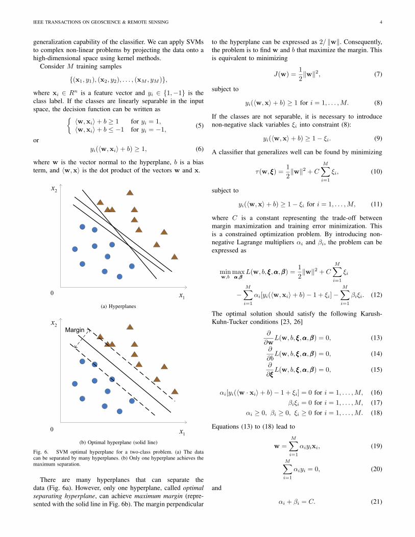
Fig. 6. SVM optimal hyperplane for a two-class problem. (a) The datacan be separated by many hyperplanes. (b) Only one hyperplane achieves themaximum separation.
There are many hyperplanes that can separate the
data (Fig. 6a). However, only one hyperplane, called optimal
separating hyperplane, can achieve maximum margin (repre-
sented with the solid line in Fig. 6b). The margin perpendicular
to the hyperplane can be expressed as 2/ ‖w‖. Consequently,
the problem is to find w and b that maximize the margin. This
is equivalent to minimizing
J(w) =1
2‖w‖2, (7)
subject to
yi(〈w,x〉+ b) ≥ 1 for i = 1, . . . ,M. (8)
If the classes are not separable, it is necessary to introduce
non-negative slack variables ξi into constraint (8):
yi(〈w,x〉+ b) ≥ 1− ξi. (9)
A classifier that generalizes well can be found by minimizing
τ(w, ξξξ) =1
2‖w‖2 + C
M∑
i=1
ξi, (10)
subject to
yi(〈w,x〉+ b) ≥ 1− ξi for i = 1, . . . ,M, (11)
where C is a constant representing the trade-off between
margin maximization and training error minimization. This
is a constrained optimization problem. By introducing non-
negative Lagrange multipliers αi and βi, the problem can be
expressed as
minw,b
maxααα,βββ
L(w, b, ξξξ,ααα,βββ) =1
2‖w‖2 + C
M∑
i=1
ξi
−M∑
i=1
αi[yi(〈w,xi〉+ b)− 1 + ξi]−M∑
i=1
βiξi. (12)
The optimal solution should satisfy the following Karush-
Kuhn-Tucker conditions [23, 26]
∂
∂wL(w, b, ξξξ,ααα,βββ) = 0, (13)
∂
∂bL(w, b, ξξξ,ααα,βββ) = 0, (14)
∂
∂ξξξL(w, b, ξξξ,ααα,βββ) = 0, (15)
αi[yi(〈w · xi〉+ b)− 1 + ξi] = 0 for i = 1, . . . ,M, (16)
βiξi = 0 for i = 1, . . . ,M, (17)
αi ≥ 0, βi ≥ 0, ξi ≥ 0 for i = 1, . . . ,M. (18)
Equations (13) to (18) lead to
w =
M∑
i=1
αiyixi, (19)
M∑
i=1
αiyi = 0, (20)
and
αi + βi = C. (21)
IEEE TRANSACTIONS ON GEOSCIENCE & REMOTE SENSING 5
Substituting Eqs. (19) to (21) into (12), the primal variables
w and b can be eliminated and a dual optimization problem
is obtained:
maximizing Q(α) =
M∑
i=1
αi −1
2
M∑
i,j=1
αiαjyiyj 〈xi,xj〉 ,
(22)
subject to
0 ≤ αi ≤ C for i = 1, . . . ,M, (23)
and
M∑
i=1
αiyi = 0 for i = 1, . . . ,M. (24)
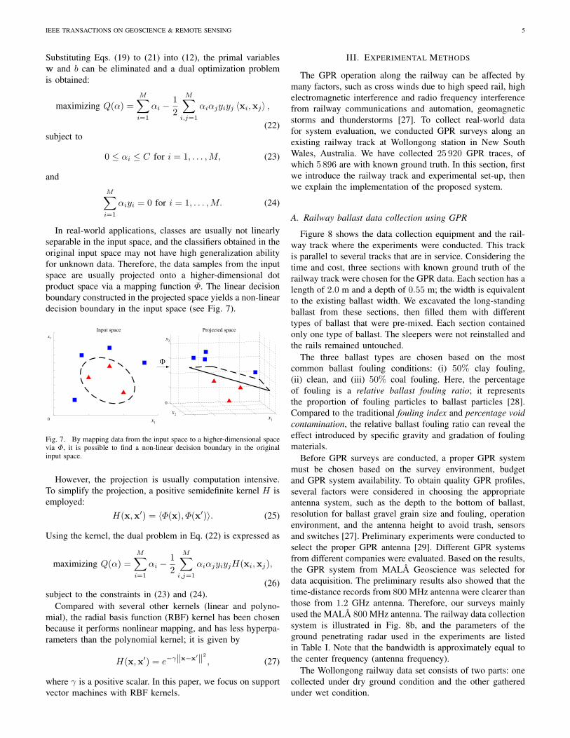
In real-world applications, classes are usually not linearly
separable in the input space, and the classifiers obtained in the
original input space may not have high generalization ability
for unknown data. Therefore, the data samples from the input
space are usually projected onto a higher-dimensional dot
product space via a mapping function Φ. The linear decision
boundary constructed in the projected space yields a non-linear
decision boundary in the input space (see Fig. 7).
Input space Projected space
1x
2x
1x2x
3x
0
0
Fig. 7. By mapping data from the input space to a higher-dimensional spacevia Φ, it is possible to find a non-linear decision boundary in the originalinput space.
However, the projection is usually computation intensive.
To simplify the projection, a positive semidefinite kernel H is
employed:
H(x,x′) = 〈Φ(x), Φ(x′)〉. (25)
Using the kernel, the dual problem in Eq. (22) is expressed as
maximizing Q(α) =
M∑
i=1
αi −1
2
M∑
i,j=1
αiαjyiyjH(xi,xj),
(26)
subject to the constraints in (23) and (24).
Compared with several other kernels (linear and polyno-
mial), the radial basis function (RBF) kernel has been chosen
because it performs nonlinear mapping, and has less hyperpa-
rameters than the polynomial kernel; it is given by
H(x,x′) = e−γ‖x−x′‖
2
, (27)
where γ is a positive scalar. In this paper, we focus on support
vector machines with RBF kernels.
III. EXPERIMENTAL METHODS
The GPR operation along the railway can be affected by
many factors, such as cross winds due to high speed rail, high
electromagnetic interference and radio frequency interference
from railway communications and automation, geomagnetic
storms and thunderstorms [27]. To collect real-world data
for system evaluation, we conducted GPR surveys along an
existing railway track at Wollongong station in New South
Wales, Australia. We have collected 25 920 GPR traces, of
which 5 896 are with known ground truth. In this section, first
we introduce the railway track and experimental set-up, then
we explain the implementation of the proposed system.
A. Railway ballast data collection using GPR
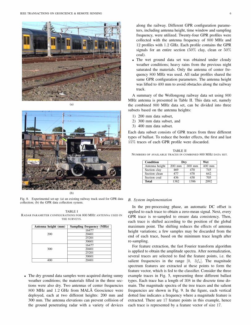
Figure 8 shows the data collection equipment and the rail-
way track where the experiments were conducted. This track
is parallel to several tracks that are in service. Considering the
time and cost, three sections with known ground truth of the
railway track were chosen for the GPR data. Each section has a
length of 2.0 m and a depth of 0.55 m; the width is equivalent
to the existing ballast width. We excavated the long-standing
ballast from these sections, then filled them with different
types of ballast that were pre-mixed. Each section contained
only one type of ballast. The sleepers were not reinstalled and
the rails remained untouched.
The three ballast types are chosen based on the most
common ballast fouling conditions: (i) 50% clay fouling,
(ii) clean, and (iii) 50% coal fouling. Here, the percentage
of fouling is a relative ballast fouling ratio; it represents
the proportion of fouling particles to ballast particles [28].
Compared to the traditional fouling index and percentage void
contamination, the relative ballast fouling ratio can reveal the
effect introduced by specific gravity and gradation of fouling
materials.
Before GPR surveys are conducted, a proper GPR system
must be chosen based on the survey environment, budget
and GPR system availability. To obtain quality GPR profiles,
several factors were considered in choosing the appropriate
antenna system, such as the depth to the bottom of ballast,
resolution for ballast gravel grain size and fouling, operation
environment, and the antenna height to avoid trash, sensors
and switches [27]. Preliminary experiments were conducted to
select the proper GPR antenna [29]. Different GPR systems
from different companies were evaluated. Based on the results,
the GPR system from MALA Geoscience was selected for
data acquisition. The preliminary results also showed that the
time-distance records from 800 MHz antenna were clearer than
those from 1.2 GHz antenna. Therefore, our surveys mainly
used the MALA 800 MHz antenna. The railway data collection
system is illustrated in Fig. 8b, and the parameters of the
ground penetrating radar used in the experiments are listed
in Table I. Note that the bandwidth is approximately equal to
the center frequency (antenna frequency).
The Wollongong railway data set consists of two parts: one
collected under dry ground condition and the other gathered
under wet condition.
IEEE TRANSACTIONS ON GEOSCIENCE & REMOTE SENSING 6
(a)
(b)
Fig. 8. Experimental set-up: (a) an existing railway track used for GPR datacollection; (b) the GPR data collection system.
TABLE IRADAR PARAMETER CONFIGURATIONS FOR 800 MHZ ANTENNA USED IN
THE SURVEYS.
Antenna height (mm) Sampling frequency (MHz)
16477200 20401
2520130601
16477300 20401
2520130601
400 20401
• The dry ground data samples were acquired during sunny
weather conditions; the materials filled in the three sec-
tions were also dry. Two antennas of center frequencies
800 MHz and 1.2 GHz from MALA Geoscience were
deployed, each at two different heights: 200 mm and
300 mm. The antenna elevations can prevent collision of
the ground penetrating radar with a variety of devices
along the railway. Different GPR configuration parame-
ters, including antenna height, time window and sampling
frequency, were utilized. Twenty-four GPR profiles were
collected with the antenna frequency of 800 MHz and
12 profiles with 1.2 GHz. Each profile contains the GPR
signals for an entire section (50% clay, clean or 50%coal).
• The wet ground data set was obtained under cloudy
weather conditions; heavy rains from the previous night
saturated the materials. Only the antenna of center fre-
quency 800 MHz was used. All radar profiles shared the
same GPR configuration parameters. The antenna height
was lifted to 400 mm to avoid obstacles along the railway
track.
A summary of the Wollongong railway data set using 800MHz antenna is presented in Table II. This data set, namely
the combined 800 MHz data set, can be divided into three
subsets based on the antenna heights:
1) 200 mm data subset,
2) 300 mm data subset, and
3) 400 mm data subset.
Each data subset consists of GPR traces from three different
types of ballast. To reduce the border effects, the first and last
15% traces of each GPR profile were discarded.
TABLE IINUMBERS OF AVAILABLE TRACES IN COMBINED 800 MHZ DATA SET.
Condition Dry Wet
Antenna height 200 mm 300 mm 400 mm
Section clay 469 470 745
Section clean 477 478 642
Section coal 436 438 705
Total 1382 1386 2092
B. System implementation
In the pre-processing phase, an automatic DC offset is
applied to each trace to obtain a zero-mean signal. Next, every
GPR trace is re-sampled to ensure data consistency. Then,
each trace is shifted according to the position of the global
maximum point. The shifting reduces the effects of antenna
height variations; a few samples may be discarded from the
end of each trace, based on the minimum trace length after
re-sampling.
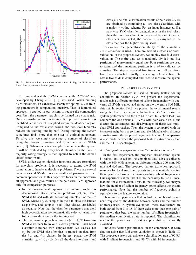
For feature extraction, the fast Fourier transform algorithm
is applied to obtain the amplitude spectra. After normalization,
several traces are selected to find the feature points, i.e. the
salient frequencies in the range [0, 3fa]. The magnitude
spectrum features are extracted at these points to form the
feature vector, which is fed to the classifier. Consider the three
example traces in Fig. 5, representing three different ballast
types. Each trace has a length of 308 in the discrete time do-
main. The magnitude spectra of the tree traces and the salient
frequencies are shown in Fig. 9. In the figure, each vertical
dotted line indicates a frequency where a magnitude feature is
extracted. There are 17 feature points in this example, hence
each trace is represented by a feature vector of size 17.
IEEE TRANSACTIONS ON GEOSCIENCE & REMOTE SENSING 7
0 500 1000 1500 2000 25000
5
10
15
20
25
Frequency (MHz)
Norm
aliz
ed m
agnitude
50% clay
clean
50% coal
Fig. 9. Feature points of the three traces shown in Fig. 3a. Each verticaldotted line represents a feature point.
To train and test the SVM classifiers, the LIBSVM tool,
developed by Chang et al. [30], was used. When building
SVM classifiers, an exhaustive search for optimal SVM train-
ing parameters is computation-intensive. Thus, a hierarchical
approach is applied in our system to reduce the computation
cost. First, the parameter search is performed on a coarse grid.
Once a possible region containing the optimal parameters is
identified, a finer search is applied within the identified region.
Compared to the exhaustive search, the two-level hierarchy
reduces the training time by half. During training, the system
sometimes finds more than one set of optimal parameters.
To solve this, we simply construct a number of classifiers
using the chosen parameters and form them as an SVMs
pool [31]. Whenever a test sample is input into the system,
it will be evaluated by every SVM classifier in the pool; a
majority voting strategy is then applied to obtain the overall
classification result.
SVMs utilize explicit decision functions and are formulated
for two-class problems. It is necessary to extend the SVM
formulation to handle multi-class problems. There are several
ways to extend SVMs; one-versus-all and pair-wise are two
common approaches. In this paper, we focus on the one-verus-
all approach, and give results of the pair-wise SVM approach
only for comparison purposes.
• In the one-versus-all approach, a k-class problem is
decomposed into k two-class problems [23, 32]. Each
SVM is trained with all the training samples. For the i-thSVM, where i ≤ k, samples in the i-th class are labeled
as positive, and samples in all other classes are labeled
as negative. Note that the classifier parameters that yield
high generalization are automatically selected using five-
fold cross-validation on the training set.
• The pair-wise approach requires k(k − 1)/2 two-class
SVM classifiers to solve a k-class problem. Each SVM
classifier is trained with samples from two classes. Let
cij be the SVM classifier that is trained on data from
the i-th and j-th classes. In the test phase, the SVM
classifier cij (i < j) divides all the data into class i and
class j. The final classification results of pair-wise SVMs
are obtained by combining all two-class classifiers with
a majority voting scheme. For an input instance x, if a
pair-wise SVM classifier categorizes x in the k-th class,
then the vote for class k is increased by one. Once all
classifiers have voted, the pattern x is assigned to the
class that has the highest voting score.
To evaluate the generalization ability of the classifiers,
cross-validation is used. There are several methods of cross-
validation; in the proposed system, we employ five-fold cross-
validation. The entire data set is randomly divided into five
partitions of approximately equal size. Four partitions are used
to train, and the remaining partition is used to validate the
classifier. The step is repeated five times until all partitions
have been evaluated. Finally, the average classification rate
across five folds is computed and used to measure the system
performance.
IV. RESULTS AND ANALYSIS
The proposed system is used to classify ballast fouling
conditions. In Section IV-A, we present the experimental
results using different numbers of salient frequencies with one-
verus-all SVMs trained and tested on the the entire 800 MHz
data set. In Section IV-B, we present the experimental results
using the three data subsets. In Section IV-C we show the
system performance on the 1.2 GHz data. In Section IV-E, we
compare the one-versus-all SVMs with pair-wise SVMs, and
discuss the advantages and disadvantages of these two multi-
class SVM approaches. Then, the system is compared with the
k-nearest neighbors algorithm and the Mahalanobis distance
classifier using the proposed magnitude feature. A comparison
is also made between the proposed feature extraction method
and the STFT spectrogram.
A. Classification performance on the combined data set
In the first experiment, the proposed classification system
is trained and tested on the combined data subsets collected
with the 800 MHz antenna at different heights: 200 mm, 300mm and 400 mm. The proposed feature extraction approach
searches for local maximum points in the magnitude spectra;
these points determine the corresponding salient frequencies.
Our experiments show that it is not necessary to use all local
maxima for classification. Thus, in the following, we analyze
how the number of salient frequency points affects the system
performance. Note that the number of frequency points is
equivalent to the feature vector size.
There are two parameters that control the number of promi-
nent frequencies: the distance between peaks and the number
of traces used. In system evaluation, these two factors are
both varied from 3 to 18. If there exist more than one pair of
parameters that bear the same number of salient frequencies,
the median classification rate is reported. The classification
rate is the percentage of test samples that are correctly
classified.
The classification performance on the combined 800 MHz
data set using five-fold cross-validation is shown in Table III.
The proposed system can achieve a classification rate of 99.5%with 7 salient frequencies, and 99.7% with 14 frequencies.
IEEE TRANSACTIONS ON GEOSCIENCE & REMOTE SENSING 8
TABLE IIICLASSIFICATION RATES FOR DIFFERENT NUMBERS OF SALIENT FREQUENCIES ON THE COMBINED 800 MHZ DATA SET.
Number of salient frequencies 7 8 10 11 14 20 24
Overall classification rate (%) 99.5 99.6 99.6 99.8 99.7 100.0 100.0
Number of salient frequencies 29 30 31 32 33 34 -
Overall classification rate (%) 100.0 100.0 100.0 100.0 100.0 100.0 -
B. Classification performance versus antenna height
Further experiments have been conducted to explore the
system performance on the three data subsets of different
antenna heights. The three experiments using 800 MHz data
set are:
1) training and testing on the 200 mm data subset,
2) training and testing on the 300 mm data subset, and
3) training and testing on the 400 mm data subset.
Since the salient frequency points are determined from the
training data, the feature vectors are different for each exper-
iment.
• The system classification performance on the 200 mm
data subset as a function of the number of salient frequen-
cies is given in Table IV. The system performance im-
proves when more frequency points are used. When fewer
than 5 frequency points are used, the classification rate
is below 80.0%. When the number of frequency points
reaches 5, the classification rate increases to 90.4%.
Once the feature size reaches 14, the system performance
remains stable with a classification rate above 99.0%.
Perfect classification is achieved with 17 frequencies or
higher.
• Table V shows the classification rates when the system
is trained on the 300 mm data subset. The classification
rate improves steadily with increasing number of salient
frequencies. When the number of salient frequencies
reaches 12, the system is able to classify the test set with
a classification rate of 99.8%.
• For 400 mm antenna height data, the system achieves an
overall classification rate of 99.7% with only 8 salient
frequencies (see Table VI); the classification rate reaches
100.0% with 10 features.
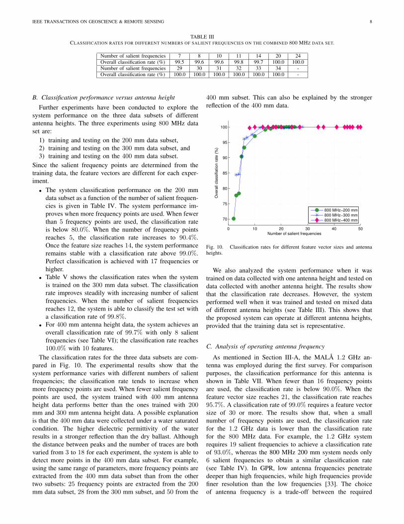
The classification rates for the three data subsets are com-
pared in Fig. 10. The experimental results show that the
system performance varies with different numbers of salient
frequencies; the classification rate tends to increase when
more frequency points are used. When fewer salient frequency
points are used, the system trained with 400 mm antenna
height data performs better than the ones trained with 200mm and 300 mm antenna height data. A possible explanation
is that the 400 mm data were collected under a water saturated
condition. The higher dielectric permittivity of the water
results in a stronger reflection than the dry ballast. Although
the distance between peaks and the number of traces are both
varied from 3 to 18 for each experiment, the system is able to
detect more points in the 400 mm data subset. For example,
using the same range of parameters, more frequency points are
extracted from the 400 mm data subset than from the other
two subsets: 25 frequency points are extracted from the 200mm data subset, 28 from the 300 mm subset, and 50 from the
400 mm subset. This can also be explained by the stronger
reflection of the 400 mm data.
0 10 20 30 40 50
70
75
80
85
90
95
100
Number of salient frequencies
Ove
rall
cla
ssifia
tio
n r
ate
(%
)
800 MHz−200 mm
800 MHz−300 mm
800 MHz−400 mm
Fig. 10. Classification rates for different feature vector sizes and antennaheights.
We also analyzed the system performance when it was
trained on data collected with one antenna height and tested on
data collected with another antenna height. The results show
that the classification rate decreases. However, the system
performed well when it was trained and tested on mixed data
of different antenna heights (see Table III). This shows that
the proposed system can operate at different antenna heights,
provided that the training data set is representative.
C. Analysis of operating antenna frequency
As mentioned in Section III-A, the MALA 1.2 GHz an-
tenna was employed during the first survey. For comparison
purposes, the classification performance for this antenna is
shown in Table VII. When fewer than 16 frequency points
are used, the classification rate is below 90.0%. When the
feature vector size reaches 21, the classification rate reaches
95.7%. A classification rate of 99.0% requires a feature vector
size of 30 or more. The results show that, when a small
number of frequency points are used, the classification rate
for the 1.2 GHz data is lower than the classification rate
for the 800 MHz data. For example, the 1.2 GHz system
requires 19 salient frequencies to achieve a classification rate
of 93.0%, whereas the 800 MHz 200 mm system needs only
6 salient frequencies to obtain a similar classification rate
(see Table IV). In GPR, low antenna frequencies penetrate
deeper than high frequencies, while high frequencies provide
finer resolution than the low frequencies [33]. The choice
of antenna frequency is a trade-off between the required
IEEE TRANSACTIONS ON GEOSCIENCE & REMOTE SENSING 9
TABLE IVCLASSIFICATION RATES FOR DIFFERENT NUMBERS OF SALIENT FREQUENCIES. DATA SET: fa = 800 MHZ, h = 200 MM.
Number of salient frequencies 2 3 4 5 6 10 14 16
Overall classification rate (%) 70.1 77.7 78.4 90.4 93.3 97.1 99.1 99.5
Number of salient frequencies 17 18 19 20 22 23 24 25
Overall classification rate (%) 100.0 100.0 100.0 100.0 100.0 100.0 100.0 100.0
TABLE VCLASSIFICATION RATES FOR DIFFERENT NUMBERS OF SALIENT FREQUENCIES. DATE SET: fa = 800 MHZ, h = 300 MM.
Number of salient frequencies 3 4 5 6 7 9 12
Overall classification rate (%) 84.4 84.6 90.5 96.1 96.6 97.5 99.8
Number of salient frequencies 13 21 23 24 26 27 28
Overall classification rate (%) 99.8 99.8 99.8 99.8 99.9 100.0 100.0
TABLE VICLASSIFICATION RATES FOR DIFFERENT NUMBERS OF SALIENT FREQUENCIES. DATE SET: fa = 800 MHZ, h = 400 MM.
Number of salient frequencies 8 10 13 15 17 18 20 24 27
Overall classification rate (%) 99.7 100.0 100.0 100.0 100.0 100.0 100.0 100.0 100.0
Number of salient frequencies 34 36 41 44 45 46 47 49 50
Overall classification rate (%) 100.0 100.0 100.0 100.0 100.0 100.0 100.0 100.0 100.0
TABLE VIICLASSIFICATION RATES FOR DIFFERENT NUMBERS OF SALIENT FREQUENCIES. DATA SET: fa = 1.2 GHZ, h = 200 MM.
Number of salient frequencies 4 7 8 9 10 11 12 15 16 19 21
Overall classification rate (%) 48.3 77.5 77.2 75.9 83.2 86.2 84.8 88.1 88.1 93.0 95.7
Number of salient frequencies 24 25 26 27 28 29 30 31 32 34 -
Overall classification rate (%) 95.4 96.7 94.1 97.1 94.4 97.6 99.4 99.4 98.9 99.4 -
depth and resolution. In this case, the results indicate that the
1.2 GHz antenna is not as good as the 800 MHz antenna.
D. Analysis of SVM design
This section compares the performances of one-versus-all
and pair-wise SVMs. With the one-versus-all SVM approach,
if a sample is classified as positive by more than one classifier
or negative by all classifiers, it will be labeled as unclassi-
fied. The unclassifiable regions of the one-versus-all approach
are shown in Fig. 11. Pair-wise SVMs, on the other hand,
have a smaller unclassifiable area compared to one-versus-
all SVMs [23]. When a new ballast class is added to the
system, the one-versus-all approach requires re-training all the
classifiers, while the pair-wise approach involves training new
classifiers between the added class and existing classes only.
1x
2x
50% clay
ballast Clean
ballast
50% coal
ballast
0
Fig. 11. An example of unclassifiable regions using one-versus-all SVMs.The solid lines are the class boundaries and the shaded regions represent theunclassifiable areas.
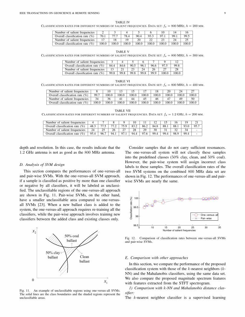
Consider samples that do not carry sufficient resonances.
The one-versus-all system will not classify these samples
into the predefined classes (50% clay, clean, and 50% coal).
However, the pair-wise system will assign incorrect class
labels to these samples. The overall classification rates of the
two SVM systems on the combined 800 MHz data set are
shown in Fig. 12. The performances of one-versus-all and pair-
wise SVMs are nearly the same.
5 10 15 20 25 30 3598.5
99
99.5
100
Number of salient frequencies
Cla
ssifia
tio
n r
ate
(%
)
One−versus−all
Pair−wise
Fig. 12. Comparison of classification rates between one-versus-all SVMsand pair-wise SVMs.
E. Comparison with other approaches
In this section, we compare the performance of the proposed
classification system with those of the k-nearest neighbors (k-
NN) and the Mahalanobis classifiers, using the same data set.
We also compare the proposed magnitude spectrum features
with features extracted from the STFT spectrogram.
1) Comparison with k-NN and Mahalanobis distance clas-
sifier:
The k-nearest neighbor classifier is a supervised learning

IEEE TRANSACTIONS ON GEOSCIENCE & REMOTE SENSING 10
algorithm based on sample distances [18]. It classifies a new
sample by searching for the closest training samples. The
label of the new sample is decided via a majority voting
scheme based on the labels of the k nearest neighbors. In
our implementation, k was varied from 1 to 17 in steps of 2.
The Mahalanobis distance is a statistical distance measure
that takes into account correlation between variables. First,
the mean mi and the covariance matrix Ci of each class are
computed from the training population. For an observation x
to be classified, the Mahalanobis distance between x and each
class is computed as follows:
Di(x,mi) =
√
(x−mi)C−1
i (x−mi)T . (28)
where i denotes the class index. The sample x is assigned to
the class with the smallest Mahalanobis distance; that is, the
index of the winning class i∗ is given by
i∗ = argmini
(Di). (29)
For comparison, five-fold cross-validation was applied. The
number of frequencies for the three 800 MHz data subsets
were 10, 9, and 8, respectively. Parameter k for the k-NN
classifier was chosen based on the training data set.
The results are shown in Fig. 13. For the 200 mm and
400 mm antenna heights, the overall classification rates of
the k-NN classifier are superior to those of the Mahalanobis
distance classifier. With the 300 mm antenna height data, the
k-NN classifier and the Mahalanobis distance classifier have
close performance. For all the data subsets, the one-versus-
all SVMs outperform both the k-NN and the Mahalanobis
distance classifier in terms of overall classification rate. For
example, on the 300 mm data subset, the SVM classifier
achieves a classification rate of 97.5%, while the k-NN and
the Mahalanobis distance classifiers reach 95.1% and 94.9%,
respectively.
97.197.5
99.7
94.895.1
96.8
88.7
94.9
82.7
80.0
84.0
88.0
92.0
96.0
100.0
200 mm 300 mm 400 mm
Ov
era
ll c
lass
ific
ati
on
ra
te (
%)
Antenna height
SVMs
k-NN
Mahalanobis distance
Fig. 13. Comparison of SVM, k-NN (k = 15) and Mahalanobis distanceclassifiers. Data set: f = 800 MHz.
2) Comparison with STFT spectrogram:
In [9], Al-Qadi et al. proposed a time-frequency approach
using short-time Fourier transform. The energy attenuation
of STFT spectrogram is utilized to assess ballast conditions.
However, their approach requires visual inspection. Here, we
are interested in the classification performance of the STFT
spectrogram features when used in the proposed system.
Our STFT spectrogram implementation is shown in Fig. 14.
The GPR traces are pre-processed, and the discrete-time STFT
is then applied to obtain the spectrogram. The discrete-time
STFT is defined as
X(m,ω) =
∞∑
n=−∞
x[n]w[n−m]e−jωn, (30)
where X(m,ω) is the STFT of windowed data, x[n] is a GPR
trace, and w[n] is a window function. The spectrogram is
represented by a 2-D matrix whereas the SVMs accept a 1-D
feature vector only. Therefore, the spectrogram is converted
into a row vector. Furthermore, considering the computational
complexity, we downsample the row vector to a feature vector
of 16, 32, 64, 128 or 256 elements. Next, the extracted feature
vectors are used as inputs to one-versus-all SVMs.
The results on the combined 800 MHz data set are shown
in Table VIII. The STFT spectrogram requires 128 frequency
points to achieve an overall classification rate of 92.9%; while
the proposed magnitude spectra yield a classification rate of
99.5% using only 7 frequency points.
GPR tracesPre-
processing
STFT
spectrogram
Output
(railway ballast
conditions)
Downsampling SVMs
Fig. 14. Block diagram of the STFT spectrogram implementation.
TABLE VIIICLASSIFICATION RATES FOR STFT SPECTROGRAM FEATURE. DATA SET:
COMBINED 800 MHZ DATA SET.
Feature vector size 16 32 64 128 256
Overall classification rate (%) 68.3 70.8 76.0 92.9 88.1
V. CONCLUSION
Compared with the traditional approach, GPR provides a
non-destructive and mobile means for fouling assessment of
railway ballast. In this paper, we have presented an automatic
classification system for GPR traces. The proposed system
is based on magnitude spectrum analysis and support vector
machines; it automates the entire GPR signal processing
and interpretation. Real-world railway data of three common
ballast fouling conditions (clean ballast, 50% clay ballast and
50% coal ballast) were collected to evaluate the proposed
system. We have made the comparison between the pro-
posed salient magnitude spectra and the STFT spectrogram,
and between SVMs and other two common classifiers. The
experimental results indicate that (i) the proposed salient
spectrum amplitudes are an efficient representation of ground
penetrating radar signals; (ii) the system performs well in
ballast fouling classification, for example, on the combined
800 MHz data set, the system can achieve a classification
rate of 99.5% using 7 salient frequencies; and (iii) the system
can operate with different antenna heights, such as 200 mm,
300 mm and 400 mm, provided that the training data set is
representative of antenna height variations.

IEEE TRANSACTIONS ON GEOSCIENCE & REMOTE SENSING 11
ACKNOWLEDGMENTS
This work is supported in part by a grant from the Australian
Research Council. The railway GPR data were collected as
part of the Rail CRC-AT5 project, sponsored by CRC Rail for
Innovation.
REFERENCES
[1] A. P. Annan, “GPR - history, trends, and future devel-
opments,” Subsurface Sensing Technologies and Appli-
cations, vol. 3, no. 4, pp. 253–270, 2002.
[2] D. J. Daniels, Ed., Ground Penetrating Radar, 2nd ed.
London: The Institution of Electrical Engineers, 2004.
[3] D. J. Daniels, D. J. Gunton, and H. F. Scott, “Introduction
to subsurface radar,” IEE Proceedings F, Radar and
Signal Processing, vol. 135, no. 4, pp. 278–320, 1988.
[4] A. Neal, “Ground-penetrating radar and its use in sed-
imentology: principles, problems and progress,” Earth-
Science Reviews, vol. 66, no. 3-4, pp. 261–330, 2004.
[5] M. Skolnik, Ed., Radar Handbook, 3rd ed. New York:
McGraw-Hill, 2008.
[6] A. Denis, F. Huneau, S. Hoerl, and A. Salomon, “GPR
data processing for fractures and flakes detection in
sandstone,” Journal of Applied Geophysics, vol. 68, no. 2,
pp. 282–288, 2009.
[7] J. J. Degenhardt Jr, “Development of tongue-shaped
and multilobate rock glaciers in alpine environments -
interpretations from ground penetrating radar surveys,”
Geomorphology, vol. 109, no. 3-4, pp. 94–107, 2009.
[8] J. Francke, “Applications of GPR in mineral resource
evaluations,” in 13th International Conference on Ground
Penetrating Radar (GPR), 2010, pp. 1–5.
[9] I. L. Al-Qadi, W. Xie, and R. Roberts, “Time-frequency
approach for ground penetrating radar data analysis to
assess railroad ballast condition,” Research in Nonde-
structive Evaluation, vol. 19, no. 4, pp. 219 – 237, 2008.
[10] J. P. Hyslip, S. S. Smith, G. R. Olhoeft, and E. T.
Selig, “Assessment of railway track substructure con-
dition using ground penetrating radar,” in 2003 Annual
Conference of AREMA, Chicago, 2003.
[11] A. Loizos and C. Plati, “Ground penetrating radar: A
smart sensor for the evaluation of the railway trackbed,”
in IEEE Instrumentation and Measurement Technology
Conference Proceedings, 2007, pp. 1–6.
[12] J. M. Reynolds, An Introduction to Applied and Environ-
mental Geophysics. New York: John Wiley, 1996.
[13] H. M. Jol, Ed., Ground Penetrating Radar Theory and
Applications, 1st ed. Amsterdam: Elsevier Science,
2009.
[14] A. M. Zoubir, I. J. Chant, C. L. Brown, B. Barkat,
and C. Abeynayake, “Signal processing techniques for
landmine detection using impulse ground penetrating
radar,” IEEE Sensors Journal, vol. 2, no. 1, pp. 41–51,
2002.
[15] S. Sinha, P. S. Routh, P. D. Anno, and J. P. Castagna,
“Spectral decomposition of seismic data with continuous-
wavelet transform,” Geophysics, vol. 70, no. 6, pp. 19–
25, 2005.
[16] M. Fujimoto, K. Nonami, A. Tatsuo, Y. Shigeru, and
M. Kazuhisa, “Mine detection algorithm using pattern
classification method by sensor fusion–experimental re-
sults by means of GPR,” in Systems and Human Science.
Amsterdam: Elsevier Science, 2005, pp. 259–274.
[17] B. J. Allred, J. J. Daniels, and M. R. Ehsani, Eds.,
Handbook of Agricultural Geophysics. Hoboken: CRC
Press, 2008.
[18] C. M. Bishop, Pattern Recognition and Machine Learn-
ing. New York: Springer, 2006.
[19] R. O. Duda, P. E. Hart, and D. G. Stork, Pattern Classi-
fication, 2nd ed. New York: Wiley, 2001.
[20] S. L. Phung, A. Bouzerdoum, and D. Chai, “Skin seg-
mentation using color pixel classification: analysis and
comparison,” IEEE Transactions on Pattern Analysis and
Machine Intelligence, vol. 27, no. 1, pp. 148–154, 2005.
[21] S. L. Phung and A. Bouzerdoum, “A new image feature
for fast detection of people in image,” International
Journal of Information and Systems Sciences, vol. 3,
no. 3, pp. 383–391, 2007.
[22] W. Shao, G. Naghdy, and S. L. Phung, “Automatic image
annotation for semantic image retrieval,” in Lecture Notes
in Computer Science: VISUAL2007, G. Qiu, Ed. Berlin
Heidelberg: Springer-Verlag, 2007, vol. 4781, pp. 372–
381.
[23] S. Abe, Support Vector Machines for Pattern Classifica-
tion. New York: Springer, 2005.
[24] N. Cristianini and J. Shawe-Taylor, An Introduction to
Support Vector Machines and Other Kernel-based Learn-
ing Methods. Cambridge: Cambridge University Press,
2001.
[25] M. A. Hearst, S. T. Dumais, E. Osman, J. Platt, and
B. Scholkopf, “Support vector machines,” IEEE Intelli-
gent Systems and Their Applications, vol. 13, no. 4, pp.
18–28, 1998.
[26] B. Schlkopf and A. J. Smola, Learning with Kernels:
Support Vector Machines, Regularization, Optimization,
and Beyond, 1st ed. Cambridge, MA: The MIT Press,
2001.
[27] G. R. Olhoeft, “Working in a difficult environment: GPR
sensing on the railroads,” in 2005 IEEE Antennas and
Propagation Society International Symposium, vol. 3B,
2005, pp. 108–111.
[28] B. Indraratna, L. Su, and C. Rujikiatkamjorn, “A new
parameter for classification and evaluation of railway
ballast fouling,” Canadian Geotechnical Journal, 2011,
in press.
[29] W. Shao, A. Bouzerdoum, S. L. Phung, L. Su, B. In-
draratna, and C. Rujikiatkamjorn, “Automatic classifica-
tion of GPR signals,” in XIII International Conference
on Ground Penetrating Radar, Lecce, Italy, 2010.
[30] C.-C. Chang and C.-J. Lin, LIBSVM: a library for
support vector machines, 2007. [Online]. Available:
http://www.csie.ntu.edu.tw/∼cjlin/libsvm/
[31] W. Shao, “Automatic annotation of digital photos,” Mas-
ter’s thesis, University of Wollongong, 2007.
[32] V. N. Vapnik, The Nature of Statistical Learning Theory,
2nd ed. New York: Springer, 2000.
IEEE TRANSACTIONS ON GEOSCIENCE & REMOTE SENSING 12
[33] C. Hauck and C. Kneisel, Eds., Applied Geophysics in
Periglacial Environments. Leiden: Cambridge Univer-
sity Press, 2008.
Wenbin Shao received the B.Eng degree (Com-munication Engineering) in 2003 from Northwest-ern Polytechnical University, Xi’an, China, and theM.Eng in 2007 from University of Wollongong,Wollongong, Australia. Currently he is a PhD stu-dent in the University of Wollongong.
Abdesselam Bouzerdoum is Professor of ComputerEngineering and Associate Dean (Research), Facultyof Informatics, University of Wollongong, Australia.He received the M.Sc. and Ph.D. degrees, both inelectrical engineering, from the University of Wash-ington, Seattle, USA. He joined Adelaide Universityin July 1991, and he was promoted to Senior Lec-turer (Senior Assistant Professor) in January 1995. In1998, he was appointed Associate Professor at EdithCowan University, Perth, Western Australia. In 2004,he moved to the University of Wollongong to take
up the position of Professor of Computer Engineering and Head of School ofElectrical, Computer and Telecommunications Engineering. In 2007, he wasappointed Associate Dean (Research) in the Faculty of Informatics. Since2009 he has been serving as a member of the Australian Research CouncilCollege of Experts, and Deputy Chair of the Engineering, Mathematics andInformatics Discipline since 2010.
Dr. Bouzerdoum received numerous awards and distinctions as acknowl-edgment of his research contributions. Most notable are a DistinguishedResearcher (Chercheur de Haut Niveau) Fellowship from the French Ministryof Scientific Research in 2001 to conduct research at the LAAS/CNRSin Toulouse, two Vice Chancellor’s Distinguished Researcher Awards, twoawards for Excellence in Research Leadership, three awards for Excellence inResearch Supervision, and the 2004 Chester Sall Award for best paper in IEEETrans. on Consumer Electronics (3rd prize). He held several appointments asVisiting Professor at Institut Galilee, University of Paris-13 (2004, 2005, 2007,2008 and 2010), Hong Kong University of Science and Technology (2007),and Villanova University (2010). He has published over 260 technical articlesand graduated sixteen Ph.D. and seven Research Masters students. He servedas Chair of the IEEE WA Section Signal Processing Chapter in 2004, and wasChair of the IEEE SA Section NN RIG from 1995 to 1997. From 1999 to2006, he served as Associate Editor of IEEE Transactions on Systems, Manand Cybernetics. Currently, he is an Associate Editor of three internationaljournals and a member of the governing board of the Asia Pacific NeuralNetwork Assembly. Dr. Bouzerdoum is a senior member of IEEE, and amember of the Optical Society of America and INNS.
Son Lam Phung received the B.Eng degree withfirst-class honors in 1999, and the Ph.D. degreein 2003, all in computer engineering, from EdithCowan University, Perth, Australia. He received theUniversity and Faculty Medals in 2000. Dr. Phungjoined the University of Wollongong as ResearchFellow in 2005, and is currently a Senior Lecturer inthe School of Electrical, Computer and Telecommu-nications Engineering. His general research interestsare in the areas of image and video processing,neural networks, pattern recognition and machine
learning.
Lijun Su is a Research Fellow in the departmentof Civil, Mining & Environmental Engineering atUniversity of Wollongong. He graduated from Xi’anJiaotong University in China (BEng) in 2000 andobtained Masters degree (Meng) from the same uni-versity in 2002. He obtained his PhD in GeotechnicalEngineering from the Hong Kong Polytechnic Uni-versity in 2006. His areas of expertise include consti-tutive modelling of geotechnical materials and non-destructive inspection of underground conditions.He has published over 30 articles in international
journals and conferences.
Buddhima Indraratna (FIEAust, FASCE, FGS,CEng, CPEng) is an internationally acclaimedgeotechnical researcher and consultant. After gradu-ating in Civil Engineering from Imperial College,University of London he obtained a Masters inSoil Mechanics also from Imperial College, andsubsequently earned a PhD in geotechnical engi-neering from University of Alberta, Canada. Heis currently Professor and Head, School of Civil,Mining & Environmental Engineering, University ofWollongong, Australia. His outstanding professional
contributions encompass innovations in railway geotechnology, soft clayengineering, ground improvement, environmental geotechnology and geo-hydraulics, with applications to transport infrastructure and dam engineering.Under his leadership, Centre for Geomechanics & Railway Engineering atUniversity of Wollongong has evolved to be a world class institution inground improvement and transport geomechanics, undertaking national andinternational research and consulting jobs.
Recognition of his efforts is reflected by numerous prestigious Awards, suchas: 2009 EH Davis Memorial Lecture by the Australian Geomechanics Societyfor outstanding contributions to the theory and practice of geomechanicsand Australian Commonwealth government hosted 2009 Business-HigherEducation Round Table award for Rail Track Innovations among others. He isthe author of 4 other books and over 350 publications in international journalsand conferences, including more than 30 invited keynote lectures worldwide.In the past, several of his publications have received outstanding contributionawards from International Association for Computer Methods and Advancesin Geomechanics (IACMAG), Canadian Geotechnical Society and SwedishGeotechnical Society.
Cholachat Rujikiatkamjorn is a Senior Lecturerin Civil Engineering at University of Wollongong.He is a Civil Engineering graduate from KhonkaenUniversity, Thailand (BEng) with a Masters (Meng)from the Asian Institute of Technology, Thailand.He obtained his PhD in Geotechnical Engineeringfrom the University of Wollongong. His key areas ofexpertise include ground improvement for transportinfrastructure and soft soil engineering. In 2009, hereceived an award from the International Associationfor Computer Methods and Advances in Geome-
chanics (IACMAG) for an outstanding paper by an early career researcher,and the 2006 Wollongong Trailblazer Award for innovations in soft soilstabilisation for transport infrastructure. He has published over 50 articlesin international journals and conferences.