Automated Testing of Hybrid Simulink/Stateflow Controllers:Industrial Case Studies

Reza Matinnejad, Shiva Nejati, Lionel C. BriandSnT Centre, University of Luxembourg, Luxembourg

{matinnejad,nejati,briand}@svv.lu

ABSTRACTWe present the results of applying our approach for testing Simulinkcontrollers to one public and one proprietary model, both industrial.Our approach combines explorative and exploitative search algo-rithms to visualize the controller behavior over its input space andto identify test scenarios in the controller input space that violateor are likely to violate the controller requirements. The engineers’feedback shows that our approach is easy to use in practice andgives them confidence about the behavior of their models.

CCS CONCEPTS• Software and its engineering → Software verification andvalidation;

KEYWORDSAutomotive software systems, Matlab/Simulink, testing

ACM Reference format:Reza Matinnejad, Shiva Nejati, Lionel C. Briand. 2017. Automated Testingof Hybrid Simulink/Stateflow Controllers: Industrial Case Studies. In Pro-ceedings of 2017 11th Joint Meeting of the European Software EngineeringConference and the ACM SIGSOFT Symposium on the Foundations of Soft-ware Engineering, Paderborn, Germany, September 4–8, 2017 (ESEC/FSE’17),6 pages.https://doi.org/10.1145/3106237.3117770

1 INTRODUCTIONThe Simulink/Stateflow (SL/SF) environment is widely used formodel-based design and development of control software systemsin the Cyber Physical Systems (CPSs) domain [10]. Testing SL/SFmodels is important in practice and complicated by a number of fac-tors that distinguish the testing of suchmodels from themainstreamsoftware testing applied to code: First, the inputs and outputs ofSL/SF models are signals, i.e., variables capturing evolution of valuesover time. Second, SL/SF models have continuous-time behaviorswith various signal shapes since they are expected to capture andcontinuously interact with the physical world. Finally, SL/SF models

We gratefully acknowledge funding from the European Research Council (ERC) un-der the European Union’s Horizon 2020 research and innovation programme (grantagreement No 694277).Permission to make digital or hard copies of all or part of this work for personal orclassroom use is granted without fee provided that copies are not made or distributedfor profit or commercial advantage and that copies bear this notice and the full citationon the first page. Copyrights for components of this work owned by others than ACMmust be honored. Abstracting with credit is permitted. To copy otherwise, or republish,to post on servers or to redistribute to lists, requires prior specific permission and/or afee. Request permissions from permissions@acm.org.ESEC/FSE’17, September 4–8, 2017, Paderborn, Germany© 2017 Association for Computing Machinery.ACM ISBN 978-1-4503-5105-8/17/09. . . $15.00https://doi.org/10.1145/3106237.3117770

typically have a large number of inputs and configuration parame-ters with float data types.

Engineers require tools for automated testing of Simulinkmodels.These tools would be useful in practice if they can effectively dealwith the large input spaces of controllers. Specifically, they shouldbe able (1) to visualize the behaviors of controllers over their inputspaces, and (2) to find individual test scenarios that violate or areclose to violating controller requirements. In our earlier work, wepresented automated testing techniques and tools with mechanismsfor input space exploration and exploitation [4, 6]. In this paper weapply our approach to two common types of controllers (i.e., open-loop and closed-loop controllers). In the exploration step, dependingon the number of input variables, Heatmap diagrams or regressiontrees are used to visualize the results of input space exploration.Specifically, Heatmaps are used to visualize two-dimensional inputspaces, and regression trees are used to visualize input spaces withmore than two dimensions. Both Heatmaps and regression treeshelp engineers identify critical input space regions of the modelunder test. In the exploitation step, search algorithms [3] are usedto find worst-case test scenarios of the model in critical regions ofHeatmap diagrams and critical partitions of regression trees.

Our experience of applying our approach to one public and oneproprietary model, both developed in industrial contexts, led to thefollowing observations:

- Engineers want to identify worst-case scenarios of Simulinkcontrollers to gain confidence about what risks can be expected inpractice.

- Engineers are interested in exploring controller input spaces toidentify conditions under which the risk of violating requirementsis higher.

- The overhead of applying our approach is small since it isdirectly applicable to Simulink models without requiring any trans-lation or pre-processing of the models under test.

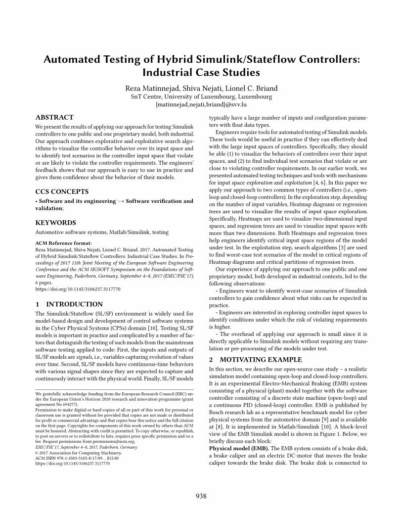
2 MOTIVATING EXAMPLEIn this section, we describe our open-source case study – a realisticsimulation model containing open-loop and closed-loop controllers.It is an experimental Electro-Mechanical Braking (EMB) systemconsisting of a physical (plant) model together with the softwarecontroller consisting of a discrete state machine (open-loop) anda continuous PID (closed-loop) controller. EMB is published byBosch research lab as a representative benchmark model for cyberphysical systems from the automotive domain [9] and is availableat [8]. It is implemented in Matlab/Simulink [10]. A block-levelview of the EMB Simulink model is shown in Figure 1. Below, webriefly discuss each block:Physical model (EMB). The EMB system consists of a brake disk,a brake caliper and an electric DC-motor that moves the brakecaliper towards the brake disk. The brake disk is connected to

938

ESEC/FSE’17, September 4–8, 2017, Paderborn, Germany Reza Matinnejad, Shiva Nejati, Lionel C. Briand

BrakeRequest( )

State-MachineController

State

Calliper Position

error

Reference Position

Inductance( )

Resistance( )EMB

Plant Model

PIDController Voltage( )

+-x(t)

x0

R

L

VBR(t)

Figure 1: Simulink model for EMB.

StartingPosition

PositionControl

ForceControl Release Force

Control

Release PositionControl

S0

S1

S2S3

S4

BR(t) == 0

BR(t) == 1

BR(t) == 1

BR(t) == 1

t + +

t + +

t + +t + +

t + +

BR(t) == 0

BR(t) == 1

R t0+t0

t0 BR(t) == t0R t00+t0

t00 BR(t) == 0

BR(t) == 0

Figure 2: The EMB state machine controller.

the wheel. The contact between the caliper and the disk resultsin vehicle deceleration. Even after the contact between the diskand caliper has been established, the DC motor can be used toexert additional braking force, allowing for fine-grained control ofthe vehicle deceleration. In Figure 1, variable x (t ) represents theposition of the caliper over time. The contact between disk andcaliper occurs at the position x0.

The EMB system is captured by the EMB Simulink plant modelin Figure 1. This model consists of mathematical equations repre-senting the relationships between the voltage applied to the motorby the controller, the motor current, the angular velocity, the angleof the motor shaft and the velocity and position of the brake caliper.The detailed equations are available in [8]. The voltage V appliedto the motor by the PID controller as well as parameters R and Lrepresenting motor resistance and motor inductance, respectively.The parameters R and L are used to create different DC motorconfigurations corresponding to different DC motor hardware.

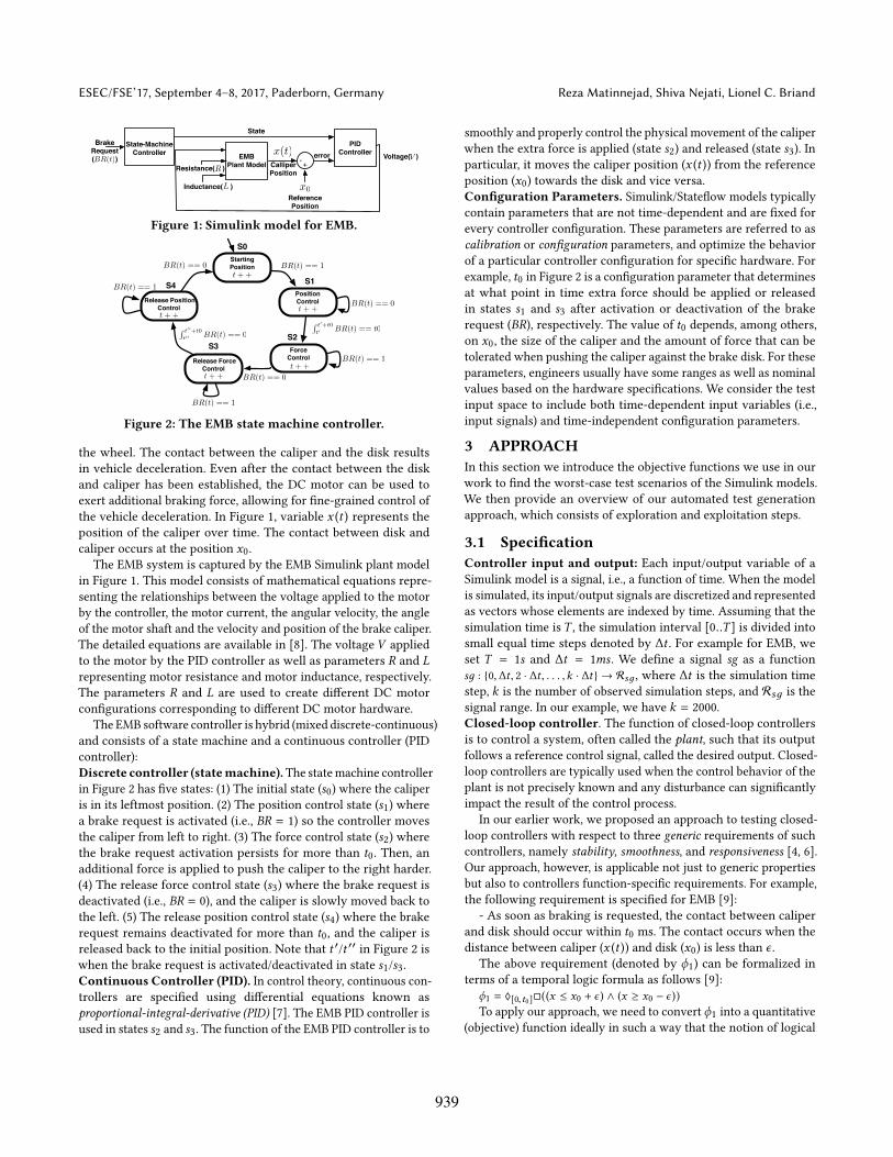
The EMB software controller is hybrid (mixed discrete-continuous)and consists of a state machine and a continuous controller (PIDcontroller):Discrete controller (statemachine).The statemachine controllerin Figure 2 has five states: (1) The initial state (s0) where the caliperis in its leftmost position. (2) The position control state (s1) wherea brake request is activated (i.e., BR = 1) so the controller movesthe caliper from left to right. (3) The force control state (s2) wherethe brake request activation persists for more than t0. Then, anadditional force is applied to push the caliper to the right harder.(4) The release force control state (s3) where the brake request isdeactivated (i.e., BR = 0), and the caliper is slowly moved back tothe left. (5) The release position control state (s4) where the brakerequest remains deactivated for more than t0, and the caliper isreleased back to the initial position. Note that t ′/t ′′ in Figure 2 iswhen the brake request is activated/deactivated in state s1/s3.Continuous Controller (PID). In control theory, continuous con-trollers are specified using differential equations known asproportional-integral-derivative (PID) [7]. The EMB PID controller isused in states s2 and s3. The function of the EMB PID controller is to

smoothly and properly control the physical movement of the caliperwhen the extra force is applied (state s2) and released (state s3). Inparticular, it moves the caliper position (x (t )) from the referenceposition (x0) towards the disk and vice versa.Configuration Parameters. Simulink/Stateflow models typicallycontain parameters that are not time-dependent and are fixed forevery controller configuration. These parameters are referred to ascalibration or configuration parameters, and optimize the behaviorof a particular controller configuration for specific hardware. Forexample, t0 in Figure 2 is a configuration parameter that determinesat what point in time extra force should be applied or releasedin states s1 and s3 after activation or deactivation of the brakerequest (BR), respectively. The value of t0 depends, among others,on x0, the size of the caliper and the amount of force that can betolerated when pushing the caliper against the brake disk. For theseparameters, engineers usually have some ranges as well as nominalvalues based on the hardware specifications. We consider the testinput space to include both time-dependent input variables (i.e.,input signals) and time-independent configuration parameters.

3 APPROACHIn this section we introduce the objective functions we use in ourwork to find the worst-case test scenarios of the Simulink models.We then provide an overview of our automated test generationapproach, which consists of exploration and exploitation steps.

3.1 SpecificationController input and output: Each input/output variable of aSimulink model is a signal, i.e., a function of time. When the modelis simulated, its input/output signals are discretized and representedas vectors whose elements are indexed by time. Assuming that thesimulation time is T , the simulation interval [0..T ] is divided intosmall equal time steps denoted by ∆t . For example for EMB, weset T = 1s and ∆t = 1ms . We define a signal sg as a functionsд : {0,∆t , 2 · ∆t , . . . ,k · ∆t } → Rsд , where ∆t is the simulation timestep, k is the number of observed simulation steps, and Rsд is thesignal range. In our example, we have k = 2000.Closed-loop controller. The function of closed-loop controllersis to control a system, often called the plant, such that its outputfollows a reference control signal, called the desired output. Closed-loop controllers are typically used when the control behavior of theplant is not precisely known and any disturbance can significantlyimpact the result of the control process.

In our earlier work, we proposed an approach to testing closed-loop controllers with respect to three generic requirements of suchcontrollers, namely stability, smoothness, and responsiveness [4, 6].Our approach, however, is applicable not just to generic propertiesbut also to controllers function-specific requirements. For example,the following requirement is specified for EMB [9]:

- As soon as braking is requested, the contact between caliperand disk should occur within t0 ms. The contact occurs when thedistance between caliper (x (t )) and disk (x0) is less than ϵ .

The above requirement (denoted by ϕ1) can be formalized interms of a temporal logic formula as follows [9]:

ϕ1 = ♢[0,t0]□((x ≤ x0 + ϵ ) ∧ (x ≥ x0 − ϵ ))

To apply our approach, we need to convert ϕ1 into a quantitative(objective) function ideally in such a way that the notion of logical

939

Automated Testing of Hybrid Simulink/Stateflow Controllers:Industrial Case Studies ESEC/FSE’17, September 4–8, 2017, Paderborn, Germany

satisfaction is preserved and can be expressed as a predicate overthe resulting quantitative function. We follow the translation of thetemporal logic formulas into quantitative functions provided by [1]for this purpose. Below, we have shown the quantitative functionobtained from ϕ1 following the translation of [1]:

F (ϕ1) = Min{Max {Max {|x (t ′) − (x0 + ϵ ) |, |x (t ′) − (x0 − ϵ ) |}}t ≤t ′≤T }0≤t ≤t0whereT is the simulation time. According to Abbas et.al. [1], we

have the following: F (ϕ1) > 2 × ϵ ⇔ ϕ1 is violatedThat is, EMB violates the property ϕ1 if and only if there is some

simulation output of EMB for which the function F (ϕ1) yields avalue larger than 2 × ϵ .Open-loop controllers: Open-loop controllers are another classof embedded controllers that control the plant in the absence ofenvironment feedback. Open-loop controllers are typically usedwhen the possible disturbances do not largely impact the controlbehavior or when it is too costly to implement the feedback mecha-nism. Figure 2 shows an example of an open-loop controller wherethe state of the caliper is computed based on the current state, timeand the brake request and not based on the feedback from the plant.For open-loop controllers, there is no plant model and feedback isnot available. For such controllers, we usually do not have require-ments such as ϕ1 since these requirements rely on the feedbackfrom the plant. In our work, to test open-loop controllers, we lookfor anti-patterns in the controller outputs, i.e., patterns indicatinga potential problem in the output signal.

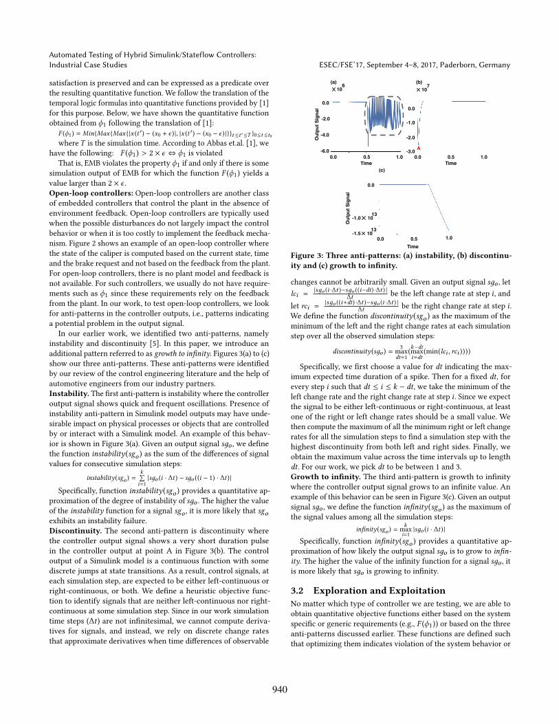
In our earlier work, we identified two anti-patterns, namelyinstability and discontinuity [5]. In this paper, we introduce anadditional pattern referred to as growth to infinity. Figures 3(a) to (c)show our three anti-patterns. These anti-patterns were identifiedby our review of the control engineering literature and the help ofautomotive engineers from our industry partners.Instability. The first anti-pattern is instability where the controlleroutput signal shows quick and frequent oscillations. Presence ofinstability anti-pattern in Simulink model outputs may have unde-sirable impact on physical processes or objects that are controlledby or interact with a Simulink model. An example of this behav-ior is shown in Figure 3(a). Given an output signal sдo , we definethe function instability (sgo ) as the sum of the differences of signalvalues for consecutive simulation steps:

instability (sgo ) =k∑i=1|sдo (i · ∆t ) − sдo ((i − 1) · ∆t ) |

Specifically, function instability (sgo ) provides a quantitative ap-proximation of the degree of instability of sдo . The higher the valueof the instability function for a signal sgo , it is more likely that sgoexhibits an instability failure.Discontinuity. The second anti-pattern is discontinuity wherethe controller output signal shows a very short duration pulsein the controller output at point A in Figure 3(b). The controloutput of a Simulink model is a continuous function with somediscrete jumps at state transitions. As a result, control signals, ateach simulation step, are expected to be either left-continuous orright-continuous, or both. We define a heuristic objective func-tion to identify signals that are neither left-continuous nor right-continuous at some simulation step. Since in our work simulationtime steps (∆t ) are not infinitesimal, we cannot compute deriva-tives for signals, and instead, we rely on discrete change ratesthat approximate derivatives when time differences of observable

0.0 0.5 1.00.0 0.5 1.0-6.0

-4.0

-2.0

0.0

(b)

Time Time

(a)

Out

put S

igna

l 0.0

-1.0

-2.0

-3.0 A

10710

6

-1.0

-1.50.0

0.0

0.5 1.0

Out

put S

igna

l

Time

1013

1013

(c)

Figure 3: Three anti-patterns: (a) instability, (b) discontinu-ity and (c) growth to infinity.

changes cannot be arbitrarily small. Given an output signal sдo , letlci =

|sдo (i ·∆t )−sдo ((i−dt) ·∆t ) |∆t be the left change rate at step i , and

let rci = |sдo ((i+dt) ·∆t )−sдo (i ·∆t ) |∆t be the right change rate at step i .

We define the function discontinuity (sgo ) as the maximum of theminimum of the left and the right change rates at each simulationstep over all the observed simulation steps:

discontinuity (sдo ) =3max

dt=1(k−dtmaxi=dt

(min(lci , rci ))))

Specifically, we first choose a value for dt indicating the max-imum expected time duration of a spike. Then for a fixed dt, forevery step i such that dt ≤ i ≤ k − dt, we take the minimum of theleft change rate and the right change rate at step i . Since we expectthe signal to be either left-continuous or right-continuous, at leastone of the right or left change rates should be a small value. Wethen compute the maximum of all the minimum right or left changerates for all the simulation steps to find a simulation step with thehighest discontinuity from both left and right sides. Finally, weobtain the maximum value across the time intervals up to lengthdt. For our work, we pick dt to be between 1 and 3.Growth to infinity. The third anti-pattern is growth to infinitywhere the controller output signal grows to an infinite value. Anexample of this behavior can be seen in Figure 3(c). Given an outputsignal sдo , we define the function infinity (sgo ) as the maximum ofthe signal values among all the simulation steps:

infinity (sgo ) =kmaxi=1|sдo (i · ∆t ) |

Specifically, function infinity (sgo ) provides a quantitative ap-proximation of how likely the output signal sдo is to grow to infin-ity. The higher the value of the infinity function for a signal sдo , itis more likely that sдo is growing to infinity.

3.2 Exploration and ExploitationNo matter which type of controller we are testing, we are able toobtain quantitative objective functions either based on the systemspecific or generic requirements (e.g., F (ϕ1)) or based on the threeanti-patterns discussed earlier. These functions are defined suchthat optimizing them indicates violation of the system behavior or

940

ESEC/FSE’17, September 4–8, 2017, Paderborn, Germany Reza Matinnejad, Shiva Nejati, Lionel C. Briand

may indicate presence of error. Our approach to test controllersbased on a given objective function has two consecutive steps:exploration and exploitation.

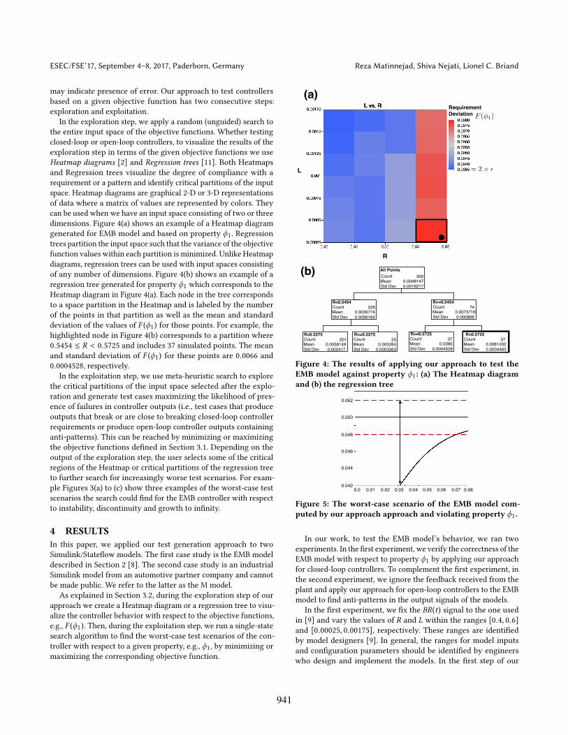
In the exploration step, we apply a random (unguided) search tothe entire input space of the objective functions. Whether testingclosed-loop or open-loop controllers, to visualize the results of theexploration step in terms of the given objective functions we useHeatmap diagrams [2] and Regression trees [11]. Both Heatmapsand Regression trees visualize the degree of compliance with arequirement or a pattern and identify critical partitions of the inputspace. Heatmap diagrams are graphical 2-D or 3-D representationsof data where a matrix of values are represented by colors. Theycan be used when we have an input space consisting of two or threedimensions. Figure 4(a) shows an example of a Heatmap diagramgenerated for EMB model and based on property ϕ1. Regressiontrees partition the input space such that the variance of the objectivefunction values within each partition is minimized. Unlike Heatmapdiagrams, regression trees can be used with input spaces consistingof any number of dimensions. Figure 4(b) shows an example of aregression tree generated for property ϕ1 which corresponds to theHeatmap diagram in Figure 4(a). Each node in the tree correspondsto a space partition in the Heatmap and is labeled by the numberof the points in that partition as well as the mean and standarddeviation of the values of F (ϕ1) for those points. For example, thehighlighted node in Figure 4(b) corresponds to a partition where0.5454 ≤ R < 0.5725 and includes 37 simulated points. The meanand standard deviation of F (ϕ1) for these points are 0.0066 and0.0004528, respectively.

In the exploitation step, we use meta-heuristic search to explorethe critical partitions of the input space selected after the explo-ration and generate test cases maximizing the likelihood of pres-ence of failures in controller outputs (i.e., test cases that produceoutputs that break or are close to breaking closed-loop controllerrequirements or produce open-loop controller outputs containinganti-patterns). This can be reached by minimizing or maximizingthe objective functions defined in Section 3.1. Depending on theoutput of the exploration step, the user selects some of the criticalregions of the Heatmap or critical partitions of the regression treeto further search for increasingly worse test scenarios. For exam-ple Figures 3(a) to (c) show three examples of the worst-case testscenarios the search could find for the EMB controller with respectto instability, discontinuity and growth to infinity.

4 RESULTSIn this paper, we applied our test generation approach to twoSimulink/Stateflow models. The first case study is the EMB modeldescribed in Section 2 [8]. The second case study is an industrialSimulink model from an automotive partner company and cannotbe made public. We refer to the latter as the M model.

As explained in Section 3.2, during the exploration step of ourapproach we create a Heatmap diagram or a regression tree to visu-alize the controller behavior with respect to the objective functions,e.g., F (ϕ1). Then, during the exploitation step, we run a single-statesearch algorithm to find the worst-case test scenarios of the con-troller with respect to a given property, e.g., ϕ1, by minimizing ormaximizing the corresponding objective function.

L

R

(a)

(b)

Requirement Deviation

All PointsCount MeanStd Dev

300 0.00481470.0016217

R<0.5454Count MeanStd Dev

226 0.00397740.0006164

R>=0.5454Count MeanStd Dev

74 0.00737160.000896

R<0.5275Count MeanStd Dev

201 0.00381490.000417

R>=0.5275Count MeanStd Dev

25 0.005284

0.0003363

R>=0.5725Count MeanStd Dev

37 0.0066

0.0004528

R<0.5725Count MeanStd Dev

37 0.00814320.0004463

= 2 ⇥ ✏

F (�1)

Figure 4: The results of applying our approach to test theEMB model against property ϕ1: (a) The Heatmap diagramand (b) the regression tree

0.01 0.02 0.03 0.04 0.05 0.06 0.07 0.080.00.042

0.044

0.046

0.048

0.050

0.052

Figure 5: The worst-case scenario of the EMB model com-puted by our approach approach and violating property ϕ1.

In our work, to test the EMB model’s behavior, we ran twoexperiments. In the first experiment, we verify the correctness of theEMB model with respect to property ϕ1 by applying our approachfor closed-loop controllers. To complement the first experiment, inthe second experiment, we ignore the feedback received from theplant and apply our approach for open-loop controllers to the EMBmodel to find anti-patterns in the output signals of the models.

In the first experiment, we fix the BR(t) signal to the one usedin [9] and vary the values of R and L within the ranges [0.4, 0.6]and [0.00025, 0.00175], respectively. These ranges are identifiedby model designers [9]. In general, the ranges for model inputsand configuration parameters should be identified by engineerswho design and implement the models. In the first step of our

941

Automated Testing of Hybrid Simulink/Stateflow Controllers:Industrial Case Studies ESEC/FSE’17, September 4–8, 2017, Paderborn, Germany

(a) All PointsCount MeanStd Dev

2384 1.016e+104.898e+11

c_gear>=1.0279Count MeanStd Dev

1997 25167.822135651.79

Count MeanStd Dev

387 6.257e+101.216e+12

t0>=0.0029462Count MeanStd Dev

1631 4550.450255698.046

t0<0.0029462Count MeanStd Dev

366 117044.69

276423.68

(b)

c_gear<1.0279

All PointsCount MeanStd Dev

999 9516636.49564029.3

In9>2737.2Count MeanStd Dev

530 994507.052353062.6

Count MeanStd Dev

469 191471883688733.9

In9<2331.1Count MeanStd Dev

480 724558.161445741.9

In9>=2331.1Count MeanStd Dev

50 3586016.45637978.5

In9<=2737.2

In9<3230.8Count MeanStd Dev

62 14112761

8077941.4

In9>=3230.8Count MeanStd Dev

407 19914103

1191847.2

In14<1Count MeanStd Dev

240 3999987.991367454.2

In14>=1Count MeanStd Dev

240 1049128.31451750.9

In1<940.09Count MeanStd Dev

40 1810628

1227440.9

In1>=940.09Count MeanStd Dev

10 10687570

9820032.9

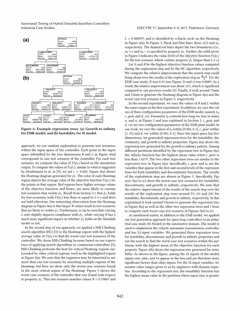
Figure 6: Example regression trees: (a) Growth-to-infinityfor EMB model, and (b) Instability for M model.

approach, we use random exploration to generate test scenarioswithin the input space of the controller. Each point in the inputspace (identified by the two dimensions R and L in Figure 4(a))corresponds to one test scenario of the controller. For each testscenario, we compute the value of F (ϕ1) based on the simulationoutput. To compute the values of F (ϕ1), similar to what is suggestedby Strathmann et al. in [9], we set ϵ = 0.002. Figure 4(a) showsthe Heatmap diagram generated for ϕ1. The color of each Heatmapregion depicts the average value of the objective function F (ϕ1) forthe points in that region. Red regions have higher average valuesof the objective function, and hence, are more likely to containtest scenarios that violate ϕ1. Recall from Section 3.1 that ϕ1 holdsfor test scenarios with F (ϕ1) less than or equal to 2 × ϵ and doesnot hold otherwise. One interesting observation from the Heatmapdiagram in Figure 4(a) is that larger R values result in test scenariosthat are likely to violate ϕ1. Furthermore, it can be seen that varyingL only slightly impacts compliance with ϕ1, while varying R has amuch more significant impact on whether ϕ1 holds on the Simulinkmodel or not.

In the second step of our approach, we applied a Hill-Climbingsearch algorithm (HC) [3] to the Heatmap region with the highestaverage value of F (ϕ1) to find the worst-case test scenarios of thecontroller. We chose Hill-Climbing because based on our experi-ence of applying search algorithms to continuous controllers [5],Hill-Climbing performs the best for critical Heatmap regions sur-rounded by other critical regions, such as the highlighted regionin Figure 4(a). We note that the engineers may be interested to seemore than one test scenario by searching multiple regions of theHeatmap, but here we show only the worst-case scenario foundin the most critical region of the Heatmap. Figure 5 shows theworst-case scenario of the controller that was found with respectto property ϕ1. This test scenario matches values R = 0.59807 and

L = 0.000297, and is identified by a black circle on the Heatmapin Figure 4(a). In Figure 5, black and blue lines show x (t ) and x0,respectively. The dashed red lines depict the two boundaries (i.e.,x0 + ϵ and x0 − ϵ) specified by property ϕ1. Further, the solid arrowin Figure 5 indicates the value (0.01) of the objective function F (ϕ1)for the test scenario, which violates property ϕ1 (larger than 2 × ϵ).

Let A and B be the highest objective function values computedduring the exploration step and by the HC algorithm, respectively.We compute the relative improvement that the search step couldbring about over the results of the exploration step as B−A

A . For theEMB case study, B was 0.01 (see Figure 5) and A was 0.0089. As aresult, the relative improvement was about 12%, which is significantcompared to our previous results [5]. Finally, it took around 75minand 15min to generate the Heatmap diagram in Figure 4(a) and theworst-case test scenario in Figure 5, respectively.

In the second experiment, we vary the values of R and L withinthe same ranges as the first experiment. In addition, we vary the val-ues of three configuration parameters of the EMB model, namely t0,c_дear and d_rot . Parameter t0 controls how long we stay in statess1 and s3 in Figure 2 and was explained in Section 2. c_дear andd_rot are two configuration parameters of the EMB plant model. Inour work, we vary the values of t0 within [0.001, 0.1], c_дear within[1, 32] and d_rot within [0.001, 0.1]. Since the input space has fivedimensions, we generated regression trees for the instability, dis-continuity, and growth to infinity properties. Figure 6(a) shows theregression tree generated for the growth to infinity pattern. Amongdifferent partitions identified by the regression tree in Figure 6(a),the infinity function has the highest mean value when c_дear isless than 1.0279. The two other regression trees are similar to theregression tree in Figure 6(a). Specifically, c_дear and t0 are thevariables that appear in the first and second levels of the regressiontrees for both instability and discontinuity functions. The resultsof the exploitation step are shown in Figure 3. Specifically, Fig-ures 3(a) to (c) show the worst-case test scenarios for instability,discontinuity, and growth to infinity, respectively. We note thatthe relative improvement of the results of the search step over theresults of the exploration step were around 5%, 6% and 24% forinstability, discontinuity and growth to infinity, respectively. In thisexperiment it took around 9 hours to generate the regression treein Figure 4(a) as well as the other two regression trees and 1 hourto compute each worst-case test scenario in Figures 3(a) to (c).

As mentioned earlier, in addition to the EMB model, we appliedour test generation approach for open-loop controllers to an indus-trial case study (M Model) in the automotive domain. The model isused to implement the vehicle automatic transmission controllerand has 24 input variables. We generated three regression treesfor instability, discontinuity and growth to infinity properties andran the search to find the worst-case test scenarios within the par-titions with the highest mean of the objective function for eachproperty. Figure 6(b) shows the regression tree generated for insta-bility. As shown in the figure, among the 24 inputs of the model,inputs one, nine, and 14 appear in the tree and are therefore moresignificant factors than other inputs. For the 24 input variables, weassume value ranges given to us by engineers with domain exper-tise. According to the regression tree, the instability function hasthe highest mean value in the partition where input nine is greater

942

ESEC/FSE’17, September 4–8, 2017, Paderborn, Germany Reza Matinnejad, Shiva Nejati, Lionel C. Briand

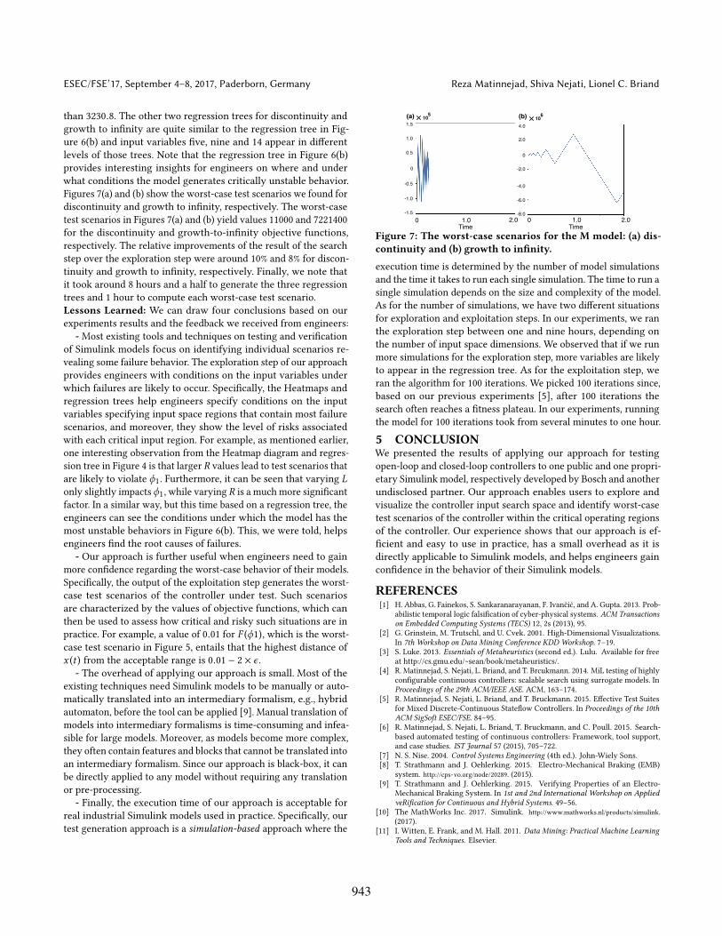
than 3230.8. The other two regression trees for discontinuity andgrowth to infinity are quite similar to the regression tree in Fig-ure 6(b) and input variables five, nine and 14 appear in differentlevels of those trees. Note that the regression tree in Figure 6(b)provides interesting insights for engineers on where and underwhat conditions the model generates critically unstable behavior.Figures 7(a) and (b) show the worst-case test scenarios we found fordiscontinuity and growth to infinity, respectively. The worst-casetest scenarios in Figures 7(a) and (b) yield values 11000 and 7221400for the discontinuity and growth-to-infinity objective functions,respectively. The relative improvements of the result of the searchstep over the exploration step were around 10% and 8% for discon-tinuity and growth to infinity, respectively. Finally, we note thatit took around 8 hours and a half to generate the three regressiontrees and 1 hour to compute each worst-case test scenario.Lessons Learned: We can draw four conclusions based on ourexperiments results and the feedback we received from engineers:

- Most existing tools and techniques on testing and verificationof Simulink models focus on identifying individual scenarios re-vealing some failure behavior. The exploration step of our approachprovides engineers with conditions on the input variables underwhich failures are likely to occur. Specifically, the Heatmaps andregression trees help engineers specify conditions on the inputvariables specifying input space regions that contain most failurescenarios, and moreover, they show the level of risks associatedwith each critical input region. For example, as mentioned earlier,one interesting observation from the Heatmap diagram and regres-sion tree in Figure 4 is that larger R values lead to test scenarios thatare likely to violate ϕ1. Furthermore, it can be seen that varying Lonly slightly impacts ϕ1, while varying R is a much more significantfactor. In a similar way, but this time based on a regression tree, theengineers can see the conditions under which the model has themost unstable behaviors in Figure 6(b). This, we were told, helpsengineers find the root causes of failures.

- Our approach is further useful when engineers need to gainmore confidence regarding the worst-case behavior of their models.Specifically, the output of the exploitation step generates the worst-case test scenarios of the controller under test. Such scenariosare characterized by the values of objective functions, which canthen be used to assess how critical and risky such situations are inpractice. For example, a value of 0.01 for F (ϕ1), which is the worst-case test scenario in Figure 5, entails that the highest distance ofx (t ) from the acceptable range is 0.01 − 2 × ϵ .

- The overhead of applying our approach is small. Most of theexisting techniques need Simulink models to be manually or auto-matically translated into an intermediary formalism, e.g., hybridautomaton, before the tool can be applied [9]. Manual translation ofmodels into intermediary formalisms is time-consuming and infea-sible for large models. Moreover, as models become more complex,they often contain features and blocks that cannot be translated intoan intermediary formalism. Since our approach is black-box, it canbe directly applied to any model without requiring any translationor pre-processing.

- Finally, the execution time of our approach is acceptable forreal industrial Simulink models used in practice. Specifically, ourtest generation approach is a simulation-based approach where the

(a) (b)

0 1.0 2.0 0 1.0 2.0

0

4.0

-4.0

-8.0

0

1.5

-1.5

1.0

-1.0

0.5

-0.5

2.0

-2.0

-6.0

105

106

Time TimeFigure 7: The worst-case scenarios for the M model: (a) dis-continuity and (b) growth to infinity.

execution time is determined by the number of model simulationsand the time it takes to run each single simulation. The time to run asingle simulation depends on the size and complexity of the model.As for the number of simulations, we have two different situationsfor exploration and exploitation steps. In our experiments, we ranthe exploration step between one and nine hours, depending onthe number of input space dimensions. We observed that if we runmore simulations for the exploration step, more variables are likelyto appear in the regression tree. As for the exploitation step, weran the algorithm for 100 iterations. We picked 100 iterations since,based on our previous experiments [5], after 100 iterations thesearch often reaches a fitness plateau. In our experiments, runningthe model for 100 iterations took from several minutes to one hour.

5 CONCLUSIONWe presented the results of applying our approach for testingopen-loop and closed-loop controllers to one public and one propri-etary Simulink model, respectively developed by Bosch and anotherundisclosed partner. Our approach enables users to explore andvisualize the controller input search space and identify worst-casetest scenarios of the controller within the critical operating regionsof the controller. Our experience shows that our approach is ef-ficient and easy to use in practice, has a small overhead as it isdirectly applicable to Simulink models, and helps engineers gainconfidence in the behavior of their Simulink models.

REFERENCES[1] H. Abbas, G. Fainekos, S. Sankaranarayanan, F. Ivančić, and A. Gupta. 2013. Prob-

abilistic temporal logic falsification of cyber-physical systems. ACM Transactionson Embedded Computing Systems (TECS) 12, 2s (2013), 95.

[2] G. Grinstein, M. Trutschl, and U. Cvek. 2001. High-Dimensional Visualizations.In 7th Workshop on Data Mining Conference KDD Workshop. 7–19.

[3] S. Luke. 2013. Essentials of Metaheuristics (second ed.). Lulu. Available for freeat http://cs.gmu.edu/~sean/book/metaheuristics/.

[4] R. Matinnejad, S. Nejati, L. Briand, and T. Brcukmann. 2014. MiL testing of highlyconfigurable continuous controllers: scalable search using surrogate models. InProceedings of the 29th ACM/IEEE ASE. ACM, 163–174.

[5] R. Matinnejad, S. Nejati, L. Briand, and T. Bruckmann. 2015. Effective Test Suitesfor Mixed Discrete-Continuous Stateflow Controllers. In Proceedings of the 10thACM SigSoft ESEC/FSE. 84–95.

[6] R. Matinnejad, S. Nejati, L. Briand, T. Bruckmann, and C. Poull. 2015. Search-based automated testing of continuous controllers: Framework, tool support,and case studies. IST Journal 57 (2015), 705–722.

[7] N. S. Nise. 2004. Control Systems Engineering (4th ed.). John-Wiely Sons.[8] T. Strathmann and J. Oehlerking. 2015. Electro-Mechanical Braking (EMB)

system. http://cps-vo.org/node/20289. (2015).[9] T. Strathmann and J. Oehlerking. 2015. Verifying Properties of an Electro-

Mechanical Braking System. In 1st and 2nd International Workshop on AppliedveRification for Continuous and Hybrid Systems. 49–56.

[10] The MathWorks Inc. 2017. Simulink. http://www.mathworks.nl/products/simulink.(2017).

[11] I. Witten, E. Frank, and M. Hall. 2011. Data Mining: Practical Machine LearningTools and Techniques. Elsevier.

943