Ar

Ka

b

a

ARA

KACKV

1

tMajpesatmai

isi

0d

Computerized Medical Imaging and Graphics 33 (2009) 359–368

Contents lists available at ScienceDirect

Computerized Medical Imaging and Graphics

journa l homepage: www.e lsev ier .com/ locate /compmedimag

utomated identification of anatomical landmarks on 3D bone modelseconstructed from CT scan images

. Subburaja, B. Ravia,∗, Manish Agarwalb

OrthoCAD Network Research Centre, Department of Mechanical Engineering, Indian Institute of Technology Bombay, Powai, Mumbai 400076, IndiaDepartment of Surgical Oncology, Tata Memorial Hospital, Parel, Mumbai 400012, India

r t i c l e i n f o

rticle history:eceived 5 February 2009ccepted 2 March 2009

eywords:natomical landmarksurvature and its derivativesneeirtual surgery planning

a b s t r a c t

Identification of anatomical landmarks on skeletal tissue reconstructed from CT/MR images is indis-pensable in patient-specific preoperative planning (tumour referencing, deformity evaluation, resectionplanning, and implant alignment and anchoring) as well as intra-operative navigation (bone registra-tion and instruments referencing). Interactive localisation of landmarks on patient-specific anatomicalmodels is time-consuming and may lack in repeatability and accuracy. We present a computer graphics-based method for automatic localisation and identification (labelling) of anatomical landmarks on a 3Dmodel of bone reconstructed from CT images of a patient. The model surface is segmented into differentlandmark regions (peak, ridge, pit and ravine) based on surface curvature. These regions are labelled auto-matically by an iterative process using a spatial adjacency relationship matrix between the landmarks.

The methodology has been implemented in a software program and its results (automatically identifiedlandmarks) are compared with those manually palpated by three experienced orthopaedic surgeons, onthree 3D reconstructed bone models. The variability in location of landmarks was found to be in the rangeof 2.15–5.98 mm by manual method (inter surgeon) and 1.92–4.88 mm by our program. Both methodsperformed well in identifying sharp features. Overall, the performance of the automated methodologywas better or similar to the manual method and its results were reproducible. It is expected to have a

surge

variety of applications in

. Introduction

Anatomical landmarks are distinct regions or points on skeletalissues with uniqueness in shape characteristics in their vicinity.

ost of the landmarks used during surgical procedures are manu-lly palpable and geometrically recognizable. For example, in kneeoint major landmarks include: on distal femur bone—most distaloint of medial and lateral condyles (MC and LC), medial and lat-ral epicondyle eminences (ME and LE), peak on medial and lateralide of anterior ridge (MP and LP) of prominent patellar groove, anddductor magnus attachment tubercle (AT); on proximal tibia—tibialuberosity (TT), Gerdy’s tubercle (GT), apex of Fibula (HF), most

edial and lateral point of tibial plateau (MP and LP), and medialnd lateral intercondylar tubercle (MIT and LIT). These are shownn Fig. 1.

Accurate localisation of 3D landmarks on skeletal tissue isndispensable in biomechanical studies and computer integratedurgery, including custom implant design and positioning [1–4],ntra-operative navigation, joint kinematics study [5–7], deformi-

∗ Corresponding author. Tel.: +91 22 2576 7510; fax: +91 22 2572 6875.E-mail addresses: b.ravi@iitb.ac.in, prof.b.ravi@gmail.com (B. Ravi).

895-6111/$ – see front matter © 2009 Elsevier Ltd. All rights reserved.oi:10.1016/j.compmedimag.2009.03.001

ry planning and intra-operative navigation.© 2009 Elsevier Ltd. All rights reserved.

ties assessment [8], tumour resection [9], referencing [10], andregistration in shape models [11] (Lorenz and Krahnstover [29]). Insituations involving tumours and highly deformed bones, patient-specific 3D anatomical models reconstructed from CT or MR imagesare used for visualisation and surgical planning (tumour local-isation, resection planning, and prosthesis positioning). Variousmethods used in current practice for localising anatomical land-marks on 3D bone models are given in Table 1 along with theissues associated with them. Variability associated with identify-ing and locating anatomical landmarks (for example, on the knee)has the potential to affect the surgical outcome. Semi-automaticmethods for landmark identification with interactive control offerthe possibility of overcoming the above problems. However, exist-ing computational approaches to landmark detection often sufferfrom a significant number of false detections [12].

Several studies have been reported on interactive localisationof landmarks on dry bone models, laser digitized data [8,13] ormedical images [3]. Van Sint Jan [14] presented a comprehensive

list of bony landmarks and described the procedure for locatingthem on a patient by palpation. Della Croce et al. [15] carried outexperimental studies on manual location of lower limb landmarkson dry bone models with a group of surgeons and concluded thatthe variations are in the range 6–25 mm. Liu et al. [8] manually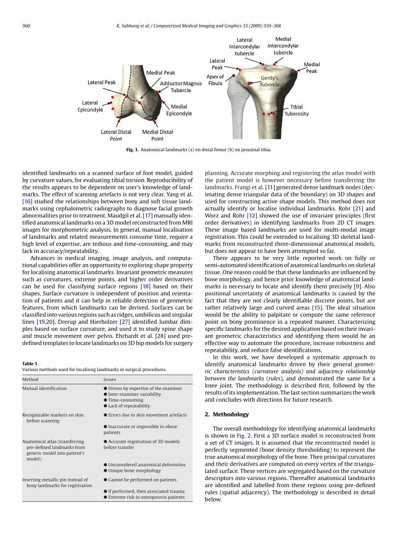

360 K. Subburaj et al. / Computerized Medical Imaging and Graphics 33 (2009) 359–368

) on di

ibtm[matiohl

tfscstfclpad

TV

M

M

R

A

I

Fig. 1. Anatomical landmarks (a

dentified landmarks on a scanned surface of foot model, guidedy curvature values, for evaluating tibial torsion. Reproducibility ofhe results appears to be dependent on user’s knowledge of land-

arks. The effect of scanning artefacts is not very clear. Yang et al.16] studied the relationships between bony and soft tissue land-

arks using cephalometric radiographs to diagnose facial growthbnormalities prior to treatment. Maudgil et al. [17] manually iden-ified anatomical landmarks on a 3D model reconstructed from MRImages for morphometric analysis. In general, manual localisationf landmarks and related measurements consume time, require aigh level of expertise, are tedious and time-consuming, and may

ack in accuracy/repeatability.Advances in medical imaging, image analysis, and computa-

ional capabilities offer an opportunity to exploring shape propertyor localising anatomical landmarks. Invariant geometric measuresuch as curvatures, extreme points, and higher order derivativesan be used for classifying surface regions [18] based on theirhapes. Surface curvature is independent of position and orienta-ion of patients and it can help in reliable detection of geometriceatures, from which landmarks can be derived. Surfaces can belassified into various regions such as ridges, umbilicus and singular

ines [19,20]. Drerup and Hierholzer [27] identified lumbar dim-les based on surface curvature, and used it to study spine shapend muscle movement over pelvis. Ehrhardt et al. [28] used pre-efined templates to locate landmarks on 3D hip models for surgery

able 1arious methods used for localising landmarks in surgical procedures.

ethod Issues

anual identification � Driven by expertise of the examiner� Inter examiner variability� Time-consuming� Lack of repeatability

ecognizable markers on skinbefore scanning

� Errors due to skin movement artefacts

� Inaccurate or impossible in obesepatients

natomical atlas (transferringpre-defined landmarks fromgeneric model into patient’smodel)

� Accurate registration of 3D modelsbefore transfer

� Unconsidered anatomical deformities� Unique bone morphology

nserting metallic pin instead ofbony landmarks for registration

� Cannot be performed on patients

� If performed, then associated trauma� Extreme risk in osteoporosis patients

stal femur (b) on proximal tibia.

planning. Accurate morphing and registering the atlas model withthe patient model is however necessary before transferring thelandmarks. Frangi et al. [11] generated dense landmark nodes (dec-imating dense triangular data of the boundary) on 3D shapes andused for constructing active shape models. This method does notactually identify or localise individual landmarks. Rohr [21] andWorz and Rohr [12] showed the use of invariant principles (firstorder derivatives) in identifying landmarks from 2D CT images.These image based landmarks are used for multi-modal imageregistration. This could be extended to localising 3D skeletal land-marks from reconstructed three-dimensional anatomical models,but does not appear to have been attempted so far.

There appears to be very little reported work on fully orsemi-automated identification of anatomical landmarks on skeletaltissue. One reason could be that these landmarks are influenced bybone morphology, and hence prior knowledge of anatomical land-marks is necessary to locate and identify them precisely [9]. Alsopositional uncertainty of anatomical landmarks is caused by thefact that they are not clearly identifiable discrete points, but arerather relatively large and curved areas [15]. The ideal situationwould be the ability to palpitate or compute the same referencepoint on bony prominence in a repeated manner. Characterizingspecific landmarks for the desired application based on their invari-ant geometric characteristics and identifying them would be aneffective way to automate the procedure, increase robustness andrepeatability, and reduce false identifications.

In this work, we have developed a systematic approach toidentify anatomical landmarks driven by their general geomet-ric characteristics (curvature analysis) and adjacency relationshipbetween the landmarks (rules), and demonstrated the same for aknee joint. The methodology is described first, followed by theresults of its implementation. The last section summarizes the workand concludes with directions for future research.

2. Methodology

The overall methodology for identifying anatomical landmarksis shown in Fig. 2. First a 3D surface model is reconstructed froma set of CT images. It is assumed that the reconstructed model isperfectly segmented (bone density thresholding) to represent thetrue anatomical morphology of the bone. Then principal curvaturesand their derivatives are computed on every vertex of the triangu-

lated surface. These vertices are segregated based on the curvaturedescriptors into various regions. Thereafter anatomical landmarksare identified and labelled from these regions using pre-definedrules (spatial adjacency). The methodology is described in detailbelow.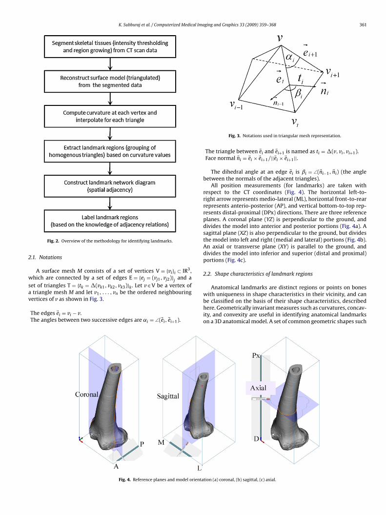

K. Subburaj et al. / Computerized Medical Imaging and Graphics 33 (2009) 359–368 361

2

wsav

Fig. 2. Overview of the methodology for identifying landmarks.

.1. Notations

A surface mesh M consists of a set of vertices V = {vi}i ⊂ IR3,hich are connected by a set of edges E = {ej = (vj1, vj2)}

jand a

et of triangles T = {tk = �(vk1, vk2, vk3)}k. Let v ∈ V be a vertex oftriangle mesh M and let v , . . . , v be the ordered neighbouring

1 n

ertices of v as shown in Fig. 3.

The edges �ei = vi − v.The angles between two successive edges are ˛i = ∠(�ei, �ei+1).

Fig. 4. Reference planes and model orienta

Fig. 3. Notations used in triangular mesh representation.

The triangle between �ei and �ei+1 is named as ti = �(v, vi, vi+1).Face normal �ni = �ei × �ei+1/||�ei × �ei+1||.

The dihedral angle at an edge �ei is ˇi = ∠(�ni−1, �ni) (the anglebetween the normals of the adjacent triangles).

All position measurements (for landmarks) are taken withrespect to the CT coordinates (Fig. 4). The horizontal left-to-right arrow represents medio-lateral (ML), horizontal front-to-rearrepresents anterio-posterior (AP), and vertical bottom-to-top rep-resents distal-proximal (DPx) directions. There are three referenceplanes. A coronal plane (YZ) is perpendicular to the ground, anddivides the model into anterior and posterior portions (Fig. 4a). Asagittal plane (XZ) is also perpendicular to the ground, but dividesthe model into left and right (medial and lateral) portions (Fig. 4b).An axial or transverse plane (XY) is parallel to the ground, anddivides the model into inferior and superior (distal and proximal)portions (Fig. 4c).

2.2. Shape characteristics of landmark regions

Anatomical landmarks are distinct regions or points on bones

with uniqueness in shape characteristics in their vicinity, and canbe classified on the basis of their shape characteristics, describedhere. Geometrically invariant measures such as curvatures, concav-ity, and convexity are useful in identifying anatomical landmarkson a 3D anatomical model. A set of common geometric shapes such

tion (a) coronal, (b) sagittal, (c) axial.

362 K. Subburaj et al. / Computerized Medical Imaging and Graphics 33 (2009) 359–368

gions:

aie

2

dmsjioi

2

asAc

2

satcmkcaaw

K

H

vnco

TD

HHH

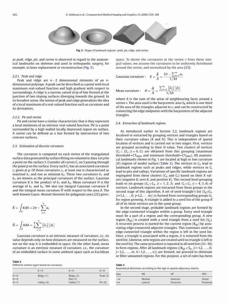
Fig. 5. Shape of landmark re

s peak, ridge, pit, and ravine is observed in regard to the anatom-cal landmarks on skeleton and used in orthopaedic surgery, forxample, in knee replacement or reconstruction (Fig. 5).

.2.1. Peak and ridgePeak and ridge are n − 2 dimensional elements of an n-

imensional polytope. A peak can be described as a point with localaximum real-valued function and high gradient with respect to

urroundings. A ridge is a narrow, raised strip of line formed at theunction of two sloping surfaces diverging towards the ground. Ints broadest sense, the notion of peak and ridge generalizes the ideaf a local maximum of a real-valued function such as curvature andts derivatives.

.2.2. Pit and ravinePit and ravine have a similar characteristic that is they represent

local minimum of an intrinsic real-valued function. Pit is a pointurrounded by a high walled locally depressed region on surface.

ravine can be defined as a line formed by intersection of twooncave surfaces.

.3. Estimation of discrete curvature

The curvature is computed on each vertex of the triangulatedurface data generated by surface fitting on volumetric data. Let p bepoint on the surface S. Consider all curves Ci on S passing through

he point p on the surface. Every such Ci has an associated curvaturei given at p. Of those curvatures ci, at least one is characterized asaximal k1 and one as minimal k2. These two curvatures k1 and

2 are known as the principal curvatures of the surface. Gaussianurvature K is the product of k1 and k2. Mean curvature H is theverage of k1 and k2. We also use integral Gaussian curvature K̄nd the integral mean curvature H̄ with respect to the area A. Theell-known Gauss–Bonnet theorem for polygonal cases [22] gives:

¯ =∫

A

KdA = 2� −n∑

i=1

˛i

¯ =∫

A

HdA = 14

n∑i=1

∥∥�ei

∥∥∣∣ˇi

∣∣

Gaussian curvature is an intrinsic measure of curvature, i.e., its

alue depends only on how distances are measured on the surface,ot on the way it is embedded in space. On the other hand, meanurvature is an extrinsic measure of curvature, i.e., the curvaturef an embedded surface in some ambient space such as Euclidean

able 2ifferent surface types based on curvature.

K < 0 K = 0 K > 0

< 0 Ridge (1) Ridge (2) Peak (3)= 0 – Flat (5) –> 0 Valley (6) Valley (7) Pit (8)

peak, pit, ridge, and ravine.

space. To derive the curvatures at the vertex v from these inte-gral values, we assume the curvatures to be uniformly distributedaround the vertex, and normalized by the area [23]:

Gaussian curvature : K = K̄

A= 2� −

∑ni=1˛i

1/3A

Mean curvature : H = H̄

A=

∑ni=1

∥∥�ei

∥∥∣∣ˇi

∣∣1/3A

where A is the sum of the areas of neighbouring faces around avertex v. The area used is the barycentric area SB which is one thirdof the area of the triangles adjacent to v, and can be constructed byconnecting the edge midpoints with the barycentres of the adjacenttriangles.

2.4. Extraction of landmark regions

As introduced earlier in Section 2.2, landmark regions arelocalised or extracted by grouping vertices and triangles based ontheir curvature values (K and H). This is independent of spatiallocation of vertices and is carried out in two stages. First, verticesare grouped according to their H value. Two clusters of vertices(Ci ⊂ ˝v, {i = h, l}) are obtained from this grouping (maximumthreshold = CTMAX and minimum threshold = CTMIN). All anatomi-cal landmarks shown in Fig. 1 are located at high or low curvature(H) regions of model surface (Table 2). The vertices in Ch lead tolandmark regions such as peaks and ridges, while vertices in Cllead to pits and valleys. Variations of specific landmark regions aresegregated from these clusters (Ch and Cl) based on their K val-ues (negative K, zero K, and positive K). This second level groupingleads to six groups (Gi ∈ Ch, {i = 1, 2, 3} and Gi ∈ Cl, {i = 4, 5, 6} ofvertices. Landmark regions are extracted from these groups in thesecond stage of this algorithm. A set of seed-triangle’s list (Sij∈Gi,{i=1,2, . . ., 6; j=1,2, . . . m}) is formed from corresponding groups Gifor region growing. A triangle is added to a seed list of the group ifall of its three vertices are in the same group.

In the second stage, probable landmark regions are formed bythe edge-connected triangles within a group. Every seed trianglemust be a part of a region and the corresponding group. A newregion (Rijk) is created with a seed triangle from a seed list (Sij).A recursive process is started for the current region (Rijk) by asso-ciating edge-connected adjacent triangles. This continues until noedge-connected triangle within the region is left in the seed list.Once, a triangle is associated with a region, it is removed from the

seed list. Likewise, new regions are created until no triangle is left inthe seed list. The same procedure is repeated in all seed lists (S1–S6)to form regions. After all landmark regions ((Rijk ∈ Sij, {i = 1,2, . . ., 6;j = 1,2, . . ., m; k = 1,2, . . ., n}) are formed, we proceed to eliminateor filter unwanted regions. For this purpose, a set of rules has been

Table 3Anatomical directions according to the sign in spatial adjacency matrix.

Sign ML AP DPx

−ve Medial Anterior Distal+ve Lateral Posterior Proximal

K. Subburaj et al. / Computerized Medical Imaging and Graphics 33 (2009) 359–368 363

Table 4Spatial adjacency matrix of distal femur landmarks.

Node Shape AT ME LE MP LP MC LCShape – Peak Peak Peak Peak Peak Peak Peak

AT Peak – L:Px M:P:Px M:P M:P:D M:Px M:P:PxME Peak M:D – M:A:D M:P M:P:D M:Px M:PxLE Peak L:A:D L:P:Px – L:P L:P:D L:Px L:PxMP Peak L:A:D L:A M:A – M:P:D L:A:Px M:A:PxL :A:PxM :DL :D

dso

A

u(asatutarl

a

L

w

s

t

TS

NS

TMLGHLM

P Peak L:A:Px L:A:Px MC Peak L:D L:D M

C Peak L:A:D L:D M

esigned based on the number of triangles associated with a region,urface area of the region, and the location of the region. The stepsf the algorithm for localising landmark regions are given below:

lgorithm. Localisation of landmark regionsInput: List of vertices (˝�) with curvature values.Output: Landmark regions RProcedure:

Step 1: set CTMax and CTMin.Step 2: get clusters Ci ⊂ ˝v, {i = h, l} by thresholding.Step 3: form groups Gi ∈ Ch, {i = 1, 2, 3} and Gi ∈ Cl, {i = 4, 5, 6}from corresponding clusters using K.Step 5: construct triangle seed lists Si j ∈ Gi, {i = 1,2, . . ., 6; j = 1,2, . . .,M}.Step 6: get landmark regions Rijk ∈ Sij, {i = 1,2, . . ., 6; j = 1,2, . . ., M;k = 1,2, . . ., N} by segmenting homogenous triangles in particularseed list.

According to differential geometry, local surface shape isniquely determined by the first and second fundamental formsDo Carmo [22]). Gaussian and mean curvature combine these firstnd second fundamental forms in two different ways to obtaincalar surface features that are invariant to rotations, translationsnd changes in parameterization [24]. There are eight fundamen-al viewpoint-independent surface types that can be characterizedsing only the sign of the mean curvature (H) and Gaussian curva-ure (K). In this work, we focus on only five surface types, whichre typically observed in anatomical models and used as landmarkegions (Table 2). A unique geometric identifier is given to eachandmark region before identifying them anatomically.

The geometric identifier for a landmark region LRi is computeds follows:

Ri = 1 + 3(1 + sgn(H, ε)) + (1 − sgn(K, ε))

here {+1 : x > ε}

gn(x, ε) = 0 : |x| ≤ ε−1 : x < ε

The geometric identifier of a landmark region is used to iden-ify the geometric shape according to Table 1. These regions are

able 5patial adjacency matrix of proximal tibia and fibula landmarks.

ode Shape TT MP LPhape – Peak Peak Peak

T Peak – L:A:D M:A:DP Peak M:P:Px – M

P Peak L:P:Px L –T Peak L:P:Px L:A:D M:A:DF Peak L:P:Px L:P:D M:P:DIT Peak P:Px L MIT Peak P:Px L M

L:A:Px – L:A:Px M:A:PxM:P:D M:P:D – M:P:DL:P:D L:P:D L:A:Px –

filtered out by surface area, geometric characteristics of the asso-ciated triangles, and spatial location of the region with respect tothe required landmarks. The extracted landmark regions have tobe identified as a set of specific anatomical landmarks of the bonebeing focussed. We have used spatial configuration of the land-marks for this purpose, which is explained in the next section.

2.5. Spatial adjacency matrix

Most of the landmarks used in surgery are palpable (in geomet-ric terms: high and low curvature regions) and vary only in sizeand spatial location depending on patient’s age, gender, ethnic-ity, etc. These anatomical landmarks are usually constrained in aspatial relationship that is the same for all models. We thereforepropose an additional characteristic for landmark identification:relative position (adjacency) of a landmark with respect to otherknown landmarks. This is captured in a network diagram, wherea node represents a landmark and an arc represents the relation-ship between two landmarks. We characterize an arc by the spatialadjacency of a landmark relative to its neighbouring landmarks.This is encoded in terms of anatomical directions and sequenceM/L:A/P:D/Px (Table 3). After all landmarks are localised using themethods described in Sections 2.2 and 2.4, the network diagramis formed. The network diagram is shown as a spatial adjacencyrelationship matrix for computational purpose. This matrix is firstfilled with vector distances between pairs of landmarks before con-verting them into a sequential code given as above. This vectordistance carries the directional information indirectly in terms ofthe sign (±). Table 3 shows the interpretation of the signed dis-tance values in terms of anatomical directions. Tables 4 and 5 showthe spatial-adjacency relations of the anatomical landmarks of theknee (Fig. 1) as a matrix. These landmarks were selected basedon instructions given in [14] and in consultation with orthopaedicsurgeons.

The spatial adjacency relationship of the landmarks given inthe above tables is used to label the anatomical landmarks afterlocalisation. We have used simplistic way of representing spatial

adjacency relationship, since incorporating average distance andstandard deviation between landmarks (used in active shape mod-els) would be superfluous for identifying anatomical landmarks.The relations between localised landmark regions are mapped one-to-one with the spatial network diagram. Implementation of the

GT HF LIT MITPeak Peak Peak Peak

M:A:D M:A:D A:D A:DM:P:Px M:A:Px M ML:P:Px L:A:Px L L– M:A L:A:D L:A:DL:P – L:P:D L:P:DM:P:Px M:A:Px – LM:P:Px M:A:Px M –

364 K. Subburaj et al. / Computerized Medical Imaging and Graphics 33 (2009) 359–368

e bon

an

3

o0wwhv

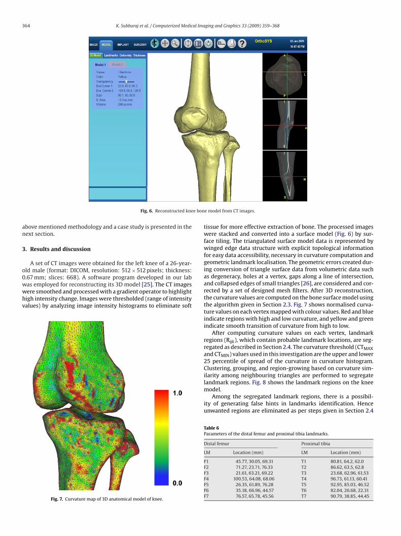
Fig. 6. Reconstructed kne

bove mentioned methodology and a case study is presented in theext section.

. Results and discussion

A set of CT images were obtained for the left knee of a 26-year-ld male (format: DICOM, resolution: 512 × 512 pixels; thickness:

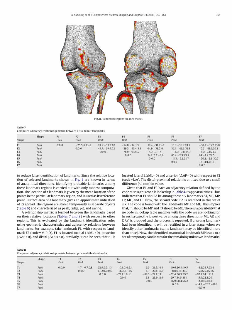
.67 mm; slices: 668). A software program developed in our labas employed for reconstructing its 3D model [25]. The CT imagesere smoothed and processed with a gradient operator to highlightigh intensity change. Images were thresholded (range of intensityalues) by analyzing image intensity histograms to eliminate soft

Fig. 7. Curvature map of 3D anatomical model of knee.

e model from CT images.

tissue for more effective extraction of bone. The processed imageswere stacked and converted into a surface model (Fig. 6) by sur-face tiling. The triangulated surface model data is represented bywinged edge data structure with explicit topological informationfor easy data accessibility, necessary in curvature computation andgeometric landmark localisation. The geometric errors created dur-ing conversion of triangle surface data from volumetric data suchas degeneracy, holes at a vertex, gaps along a line of intersection,and collapsed edges of small triangles [26], are considered and cor-rected by a set of designed mesh filters. After 3D reconstruction,the curvature values are computed on the bone surface model usingthe algorithm given in Section 2.3. Fig. 7 shows normalised curva-ture values on each vertex mapped with colour values. Red and blueindicate regions with high and low curvature, and yellow and greenindicate smooth transition of curvature from high to low.

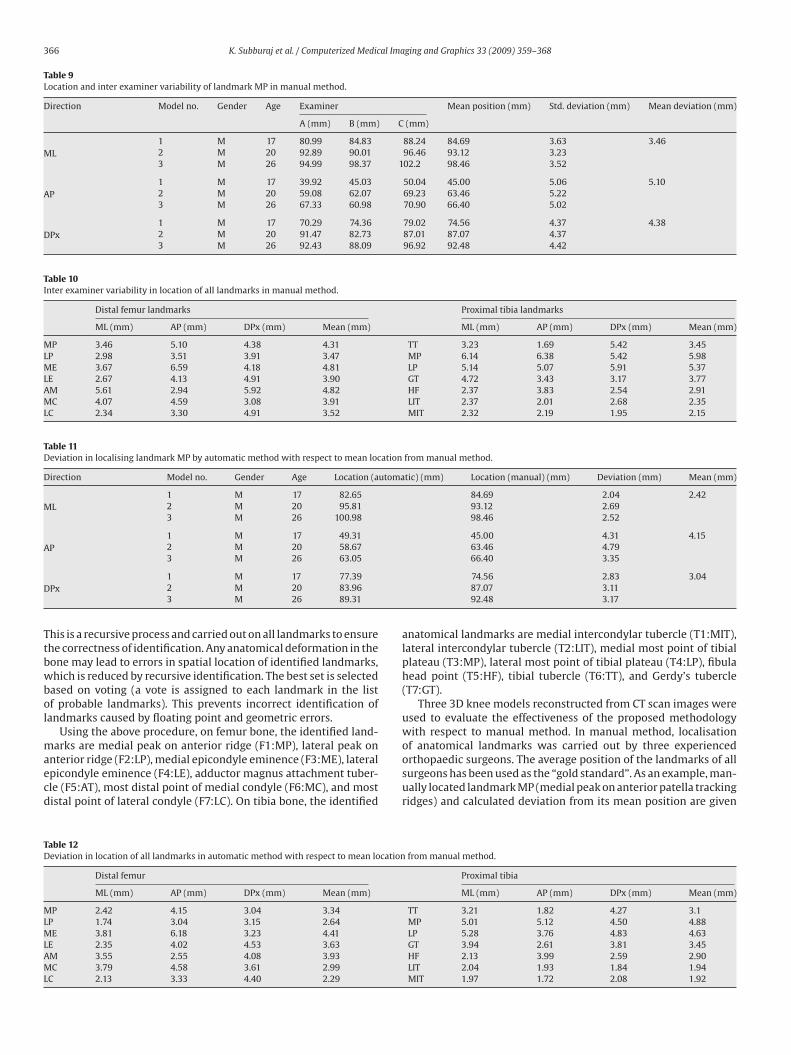
After computing curvature values on each vertex, landmarkregions (Rijk), which contain probable landmark locations, are seg-regated as described in Section 2.4. The curvature threshold (CTMAXand CTMIN) values used in this investigation are the upper and lower25 percentile of spread of the curvature in curvature histogram.Clustering, grouping, and region-growing based on curvature sim-ilarity among neighbouring triangles are performed to segregate

landmark regions. Fig. 8 shows the landmark regions on the kneemodel.

Among the segregated landmark regions, there is a possibil-ity of generating false hints in landmarks identification. Henceunwanted regions are eliminated as per steps given in Section 2.4

Table 6Parameters of the distal femur and proximal tibia landmarks.

Distal femur Proximal tibia

LM Location (mm) LM Location (mm)

F1 45.77, 30.05, 69.31 T1 80.81, 64.2, 62.0F2 71.27, 23.71, 76.33 T2 86.62, 63.5, 62.8F3 21.61, 63.21, 69.22 T3 23.68, 62.96, 61.53F4 100.53, 64.08, 68.06 T4 96.73, 61.13, 60.41F5 26.35, 61.89, 76.28 T5 92.95, 85.03, 46.52F6 35.18, 66.96, 44.57 T6 82.04, 26.68, 22.31F7 76.57, 65.78, 45.56 T7 90.79, 38.85, 44.45

K. Subburaj et al. / Computerized Medical Imaging and Graphics 33 (2009) 359–368 365

Fig. 8. Landmark regions on knee model.

Table 7Computed adjacency relationship matrix between distal femur landmarks.

Shape F1 F2 F3 F4 F5 F6 F7Shape Peak Peak Peak Peak Peak Peak Peak

F1 Peak 0:0:0 −25.5:6.3:−7 24.2:−33.2:0.1 −54.8:−34:1.3 19.4:−31.8:−7 10.6:−36.9:24.7 −30.8:−35.7:23.8F2 Peak 0:0:0 49.7:−39.5:7.1 −29.3:−40.4:8.3 44.9:−38.2:0 36.1:−43.3:31.8 −5.3:−41.6:30.8F3 Peak 0:0:0 −78.9:−0.9:1.2 −4.7:1.3:−7.1 −13.6:−3.8:24.7 −55:−2.1:23.7FFFF

ttottppo(

orulm(

TC

S

TTTTTTT

4 Peak5 Peak6 Peak7 Peak

o reduce false identification of landmarks. Since the relative loca-ion of selected landmarks shown in Fig. 1 are known in termsf anatomical directions, identifying probable landmarks amonghese landmark regions is carried out with only modest computa-ion. The location of a landmark is given by the mean location of theoints in the particular landmark region, and is used as its referenceoint. Surface area of a landmark gives an approximate indicationf its spread. The regions are stored temporarily as separate objectsTable 6) and characterized as peak, ridge, pit, and ravine.

A relationship matrix is formed between the landmarks basedn their relative locations (Tables 7 and 8) with respect to otheregions. This is evaluated by the landmark identification rules

sing geometric characteristics and adjacency relations between

andmarks. For example, take landmark F1, with respect to land-ark F2 (code = M:P:D), F1 is located medial (�ML < 0), posterior

�AP < 0), and distal (�DPx < 0). Similarly, it can be seen that F1 is

able 8omputed adjacency relationship matrix between proximal tibia landmarks.

Shape T1 T2 T3 T4hape Peak Peak Peak Peak

1 Peak 0:0:0 1.7:−0.7:0.8 62.9:0.5:1.3 −10.12 Peak 0:0:0 61.2:1.3:0.5 −11.93 Peak 0:0:0 −73.14 Peak 0:05 Peak6 Peak7 Peak

0:0:0 74.2:2.2:−8.2 65.4:−2.9:23.5 24:−1.2:22.50:0:0 −8.8:−5.1:31.7 −50.2:−3.9:30.7

0,0,0 −41.4:1.2:−10:0:0

located lateral (�ML < 0) and anterior (�AP < 0) with respect to F3(code = L:A). The distal-proximal relation is omitted due to a smalldifference (<1 mm) in value.

Given that F1 and F2 have an adjacency relation defined by thecode M:P:D, this code is looked up in Table 4. It appears 6 times. Thusindicates that F1 should be among these six landmarks AT, ME, MP,LP, MC, and LC. Now, the second code L:A is searched in this set ofsix. The code is found with the landmarks MP and ME. This impliesthat, F1 should be MP and F3 should be ME. There is a possibility thatno code in lookup table matches with the code we are looking for.In such a case, the lowest value among three directions (ML, AP, andDPx) is dropped and the process is repeated. If a wrong landmark

had been identified, it will be rectified in a later stage, when weidentify other landmarks (same landmark may be identified morethan once). Now, the identified anatomical landmark MP leads to aset of temporary candidates for the remaining unknown landmarks.

T5 T6 T7Peak Peak Peak

:2.4:2.4 −6.3:−21.5:14.3 10.6:36.8:40.5 −4.2:24.7:22.4:3.1:1.6 −8.1:−20.8:13.5 8.8:37.5:39.7 −5.9:25.4:21.6:1.8:1.1 −69.3:−22.1:13 −52.4:36.3:39.2 −67.1:24.1:21.1:0 3.8:−23.9:11.9 20.7:34.5:38.1 5.9:22.3:20

0:0:0 16.9:58.4:26.2 2.2:46.2:8.10:0:0 −14.8:−12.2:−18.1

0:0:0

366 K. Subburaj et al. / Computerized Medical Imaging and Graphics 33 (2009) 359–368

Table 9Location and inter examiner variability of landmark MP in manual method.

Direction Model no. Gender Age Examiner Mean position (mm) Std. deviation (mm) Mean deviation (mm)

A (mm) B (mm) C (mm)

ML1 M 17 80.99 84.83 88.24 84.69 3.63 3.462 M 20 92.89 90.01 96.46 93.12 3.233 M 26 94.99 98.37 102.2 98.46 3.52

AP1 M 17 39.92 45.03 50.04 45.00 5.06 5.102 M 20 59.08 62.07 69.23 63.46 5.223 M 26 67.33 60.98 70.90 66.40 5.02

DPx1 M 17 70.29 74.36 79.02 74.56 4.37 4.382 M 20 91.47 82.73 87.01 87.07 4.373 M 26 92.43 88.09 96.92 92.48 4.42

Table 10Inter examiner variability in location of all landmarks in manual method.

Distal femur landmarks Proximal tibia landmarks

ML (mm) AP (mm) DPx (mm) Mean (mm) ML (mm) AP (mm) DPx (mm) Mean (mm)

MP 3.46 5.10 4.38 4.31 TT 3.23 1.69 5.42 3.45LP 2.98 3.51 3.91 3.47 MP 6.14 6.38 5.42 5.98ME 3.67 6.59 4.18 4.81 LP 5.14 5.07 5.91 5.37LE 2.67 4.13 4.91 3.90 GT 4.72 3.43 3.17 3.77AM 5.61 2.94 5.92 4.82 HF 2.37 3.83 2.54 2.91MC 4.07 4.59 3.08 3.91 LIT 2.37 2.01 2.68 2.35LC 2.34 3.30 4.91 3.52 MIT 2.32 2.19 1.95 2.15

Table 11Deviation in localising landmark MP by automatic method with respect to mean location from manual method.

Direction Model no. Gender Age Location (automatic) (mm) Location (manual) (mm) Deviation (mm) Mean (mm)

ML1 M 17 82.65 84.69 2.04 2.422 M 20 95.81 93.12 2.693 M 26 100.98 98.46 2.52

AP1 M 17 49.31 45.00 4.31 4.152 M 20 58.67 63.46 4.793 M 26 63.05 66.40 3.35

D

Ttbwbol

maecd

TD

MLMLAML

Px1 M 17 77.392 M 20 83.963 M 26 89.31

his is a recursive process and carried out on all landmarks to ensurehe correctness of identification. Any anatomical deformation in theone may lead to errors in spatial location of identified landmarks,hich is reduced by recursive identification. The best set is selected

ased on voting (a vote is assigned to each landmark in the listf probable landmarks). This prevents incorrect identification ofandmarks caused by floating point and geometric errors.

Using the above procedure, on femur bone, the identified land-arks are medial peak on anterior ridge (F1:MP), lateral peak on

nterior ridge (F2:LP), medial epicondyle eminence (F3:ME), lateralpicondyle eminence (F4:LE), adductor magnus attachment tuber-le (F5:AT), most distal point of medial condyle (F6:MC), and mostistal point of lateral condyle (F7:LC). On tibia bone, the identified

able 12eviation in location of all landmarks in automatic method with respect to mean location

Distal femur

ML (mm) AP (mm) DPx (mm) Mean (mm)

P 2.42 4.15 3.04 3.34P 1.74 3.04 3.15 2.64E 3.81 6.18 3.23 4.41

E 2.35 4.02 4.53 3.63M 3.55 2.55 4.08 3.93C 3.79 4.58 3.61 2.99

C 2.13 3.33 4.40 2.29

74.56 2.83 3.0487.07 3.1192.48 3.17

anatomical landmarks are medial intercondylar tubercle (T1:MIT),lateral intercondylar tubercle (T2:LIT), medial most point of tibialplateau (T3:MP), lateral most point of tibial plateau (T4:LP), fibulahead point (T5:HF), tibial tubercle (T6:TT), and Gerdy’s tubercle(T7:GT).

Three 3D knee models reconstructed from CT scan images wereused to evaluate the effectiveness of the proposed methodologywith respect to manual method. In manual method, localisationof anatomical landmarks was carried out by three experienced

orthopaedic surgeons. The average position of the landmarks of allsurgeons has been used as the “gold standard”. As an example, man-ually located landmark MP (medial peak on anterior patella trackingridges) and calculated deviation from its mean position are given

from manual method.

Proximal tibia

ML (mm) AP (mm) DPx (mm) Mean (mm)

TT 3.21 1.82 4.27 3.1MP 5.01 5.12 4.50 4.88LP 5.28 3.76 4.83 4.63GT 3.94 2.61 3.81 3.45HF 2.13 3.99 2.59 2.90LIT 2.04 1.93 1.84 1.94MIT 1.97 1.72 2.08 1.92

K. Subburaj et al. / Computerized Medical Ima

Fm

ilaaul

lIocmmdcttfaIocc

mansetqfsfcwbacii

4

iass

[

[

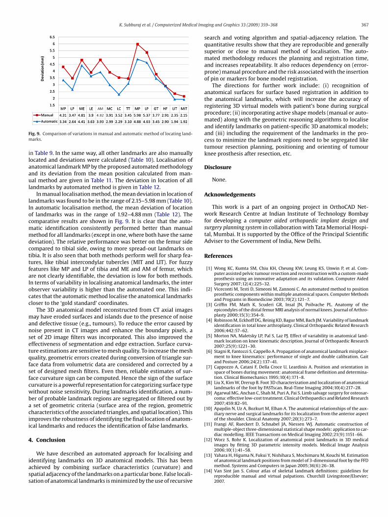
ig. 9. Comparison of variations in manual and automatic method of locating land-arks.

n Table 9. In the same way, all other landmarks are also manuallyocated and deviations were calculated (Table 10). Localisation ofnatomical landmark MP by the proposed automated methodologynd its deviation from the mean position calculated from man-al method are given in Table 11. The deviation in location of all

andmarks by automated method is given in Table 12.In manual localisation method, the mean deviation in location of

andmarks was found to be in the range of 2.15–5.98 mm (Table 10).n automatic localisation method, the mean deviation of locationf landmarks was in the range of 1.92–4.88 mm (Table 12). Theomparative results are shown in Fig. 9. It is clear that the auto-atic identification consistently performed better than manualethod for all landmarks (except in one, where both have the same

eviation). The relative performance was better on the femur sideompared to tibial side, owing to more spread-out landmarks onibia. It is also seen that both methods perform well for sharp fea-ures, like tibial intercondylar tubercles (MIT and LIT). For fuzzyeatures like MP and LP of tibia and ME and AM of femur, whichre not clearly identifiable, the deviation is low for both methods.n terms of variability in localising anatomical landmarks, the interbserver variability is higher than the automated one. This indi-ates that the automatic method localise the anatomical landmarksloser to the ‘gold standard’ coordinates.

The 3D anatomical model reconstructed from CT axial imagesay have eroded surfaces and islands due to the presence of noise

nd defective tissue (e.g., tumours). To reduce the error caused byoise present in CT images and enhance the boundary pixels, aet of 2D image filters was incorporated. This also improved theffectiveness of segmentation and edge extraction. Surface curva-ure estimations are sensitive to mesh quality. To increase the meshuality, geometric errors created during conversion of triangle sur-ace data from volumetric data are considered and corrected by aet of designed mesh filters. Even then, reliable estimates of sur-ace curvature sign can be computed. Hence the sign of the surfaceurvature is a powerful representation for categorizing surface typeithout noise sensitivity. During landmarks identification, a num-

er of probable landmark regions are segregated or filtered out byset of geometric criteria (surface area of the region, geometric

haracteristics of the associated triangles, and spatial location). Thismproves the robustness of identifying the final location of anatom-cal landmarks and reduces the identification of false landmarks.

. Conclusion

We have described an automated approach for localising anddentifying landmarks on 3D anatomical models. This has beenchieved by combining surface characteristics (curvature) andpatial adjacency of the landmarks on a particular bone. False locali-ation of anatomical landmarks is minimized by the use of recursive

[

[

ging and Graphics 33 (2009) 359–368 367

search and voting algorithm and spatial-adjacency relation. Thequantitative results show that they are reproducible and generallysuperior or close to manual method of localisation. The auto-mated methodology reduces the planning and registration time,and increases repeatability. It also reduces dependency on (error-prone) manual procedure and the risk associated with the insertionof pin or markers for bone model registration.

The directions for further work include: (i) recognition ofanatomical surfaces for surface based registration in addition tothe anatomical landmarks, which will increase the accuracy ofregistering 3D virtual models with patient’s bone during surgicalprocedure; (ii) incorporating active shape models (manual or auto-mated) along with the geometric reasoning algorithms to localiseand identify landmarks on patient-specific 3D anatomical models;and (iii) including the requirement of the landmarks in the pro-cess to minimize the landmark regions need to be segregated liketumour resection planning, positioning and orienting of tumourknee prosthesis after resection, etc.

Disclosure

None.

Acknowledgements

This work is a part of an ongoing project in OrthoCAD Net-work Research Centre at Indian Institute of Technology Bombayfor developing a computer aided orthopaedic implant design andsurgery planning system in collaboration with Tata Memorial Hospi-tal, Mumbai. It is supported by the Office of the Principal ScientificAdviser to the Government of India, New Delhi.

References

[1] Wong KC, Kumta SM, Chiu KH, Cheung KW, Leung KS, Unwin P, et al. Com-puter assisted pelvic tumour resection and reconstruction with a custom-madeprosthesis using an innovative adaptation and its validation. Computer AidedSurgery 2007;12(4):225–32.

[2] Viceconti M, Testi D, Simeoni M, Zannoni C. An automated method to positionprosthetic components within multiple anatomical spaces. Computer Methodsand Programs in Biomedicine 2003;70(2):121–7.

[3] Griffin FM, Math K, Scuderi GR, Insal JN, Poilvache PL. Anatomy of theepicondyles of the distal femur MRI analysis of normal knees. Journal of Arthro-plasty 2000;15(3):354–9.

[4] Robinson M, Eckhoff DG, Reinig KD, Bagur MM, Bach JM. Variability of landmarkidentification in total knee arthroplasty. Clinical Orthopaedic Related Research2006;442:57–62.

[5] Morton NA, Maletsky LP, Pal S, Laz PJ. Effect of variability in anatomical land-mark location on knee kinematic description. Journal of Orthopaedic Research2007;25(9):1221–30.

[6] Stagni R, Fantozzi S, Cappello A. Propagation of anatomical landmark misplace-ment to knee kinematics: performance of single and double calibration. Gaitand Posture 2006;24(2):137–41.

[7] Cappozzo A, Catani F, Della Croce U, Leardinis A. Position and orientation inspace of bones during movement: anatomical frame definition and determina-tion. Clinical Biomechanics 1995;10(4):171–8.

[8] Liu X, Kim W, Drerup B. Foot 3D characterization and localization of anatomicallandmarks of the foot by FASTscan. Real-Time Imaging 2004;10(4):217–28.

[9] Agarwal MG, Anchan C, Shah M, Puri A, Pai S. Limb salvage surgery for osteosar-coma: effective low-cost treatment. Clinical Orthopaedics and Related Research2007;459:82–91.

10] Apaydin N, Uz A, Bozkurt M, Elhan A. The anatomical relationships of the aux-iliary nerve and surgical landmarks for its localization from the anterior aspectof the shoulder. Clinical Anatomy 2007;20(3):273–7.

[11] Frangi AF, Rueckert D, Schnabel JA, Niessen WJ. Automatic construction ofmultiple-object three-dimensional statistical shape models: application to car-diac modelling. IEEE Transactions on Medical Imaging 2002;21(9):1151–66.

12] Worz S, Rohr K. Localization of anatomical point landmarks in 3D medicalimages by fitting 3D parametric intensity models. Medical Image Analysis2006;10(1):41–58.

13] Yahara H, Higuma N, Fukui Y, Nishihara S, Mochimaru M, Kouchi M. Estimationof anatomical landmark positions from model of 3-dimensional foot by the FFDmethod. Systems and Computers in Japan 2005;36(6):26–38.

14] Van Sint Jan S. Colour atlas of skeletal landmark definitions: guidelines forreproducible manual and virtual palpations. Churchill Livingstone/Elsevier;2007.

3 al Ima

[

[

[

[

[

[

[

[

[

[

[

[

[

[

[

versity of Bombay in 1987 and 1992 respectively. His main interest is limb salvagesurgery for bone and soft tissue tumours. He is a member of the musculoskeletal

68 K. Subburaj et al. / Computerized Medic

15] Della Croce U, Cappozzo A, Kerrigan DC. Pelvis and lower limb anatomicallandmark calibration precision and its propagation to bone geometry andjoint angles. Medical and Biological Engineering and Computing 1999;37(1):155–61.

16] Yang J, Ling X, Lu Y, Wei M, Ding G. Cephalometric image analysis and mea-surement for orthognathic surgery. Medical and Biological Engineering andComputing 2001;39(3):279–84.

17] Maudgil DD, Free SL, Sisodiya SM, Lemieux L, Woermann FG, Fish DR, et al.Identifying homologous anatomical landmarks on reconstructed magnetic res-onance images of the human cerebral cortical surface. Journal of Anatomy1998;193(4):559–71.

18] Koenderink J, Dooen AV. Surface shape and curvature scales. Image and VisionComputing 1992;10(8):557–65.

19] Maekawa T, Wolter EE, Patrikalakis NM. Umbilics and lines of curvature forshape interrogation. Computer Aided Geometric Design 1996;13(2):133–61.

20] Page DL, Sun Y, Koschan AF, Paik J, Abidi MA. Normal vector voting: creasedetection and curvature estimation on large, noisy meshes. Graphical Models2002;64(3-4):199–229.

21] Rohr K. Extraction of 3D anatomical point landmarks based on invariance prin-ciples. Pattern Recognition 1999;32(1):3–15.

22] Do Carmo MP. Differential geometry of curves and surfaces. New Jersey: Pren-tice Hall; 1976.

23] Meyer M, Desbrun M, Schröder P, Barr AH. Discrete differential-geometry oper-ators for triangulated 2-manifolds. Visualization and Mathematics 2002:35–57.

24] Besl PJ, Jain RC. Segmentation through variable-order surface fitting. IEEE Pat-tern Analysis and Machine Intelligence 1988;10(2):167–92.

25] Subburaj K, Ravi B. High resolution medical models and geometric reasoningstarting from CT/MR images. In: Wang G, Li H, Zha H, Zhou B, editors. Pro-ceedings of 10th IEEE International Conference on Computer Aided Design and

Computer Graphics. Beijing: IEEE Computer Society; 2007. p. 441–4.

26] Nagy MS, Matyasi GY. Analysis of STL files. Mathematical and Computer Mod-elling 2003;38:945–60.

27] Drerup B, Hierholzer E. Automatic localization of anatomical landmarks on theback surface and construction of a body-fixed coordinate system. Journal ofBiomechanics 1987;20(10):961–70.

ging and Graphics 33 (2009) 359–368

28] Ehrhardt J, Handels H, Plotz W, Poppl SJ. Atlas-based recognition of anatomi-cal structures and landmarks and the automatic computation of orthopaedicparameters to support the virtual planning of hip operations. Methods of Infor-mation in Medicine 2004;43(4):391–7.

29] Lorenz C, Krahnstover N. Generation of point-based 3D statistical shapemodels for anatomical objects. Computer Vision and Image Understanding2000;77(2):175–91.

K. Subburaj is a PhD scholar in the Department of Mechanical Engineering, IndianInstitute of Technology Bombay, India and attached to the OrthoCAD NetworkResearch Centre. He received his M.Eng from the M.S. University of Baroda, India in2005. His current research interests are BioCAD, 3D Geometric Reasoning, SurgeryPlanning, and Rapid Prototyping.

Dr. B. Ravi is a professor of Mechanical Engineering at IIT Bombay and Founder-coordinator of OrthoCAD Network Research Centre. He completed his engineeringdegree from National Institute of Technology, Rourkela in 1986, followed by mas-ters and PhD from Indian Institute of Science, Bangalore in 1992. His areas ofresearch include casting design and simulation, product lifecycle engineering, andBio-CAD/CAM. He has published about 160 technical papers, and given over 100invited talks. He is a reviewer for ASME, IEEE, IJAMS, and IJPR. He is a memberof ASME Bio Manufacturing Committee, and Fellow of the Institution of Engineers(India).

Dr. Manish Agarwal is an orthopaedic oncologist and associate professor at TataMemorial Hospital, Mumbai. He completed his MBBS and MS (Ortho) from Uni-

tumor society of North America and has several publications in peer reviewed jour-nals. His current research includes development of an indigenous tumor prostheticsystem as well as clinical trials with herbs like Curcumin and ashwagandha for bonesarcomas.