automated construction of dynamic models of subcellular...
TRANSCRIPT

Automated construction of dynamic models of subcellular structure
Taráz E. Buck
October 2013
CMU-CB-13-105
School of Computer Science Carnegie Mellon University
Pittsburgh, PA 15213
Thesis Committee: Robert F. Murphy, Advisor
Gustavo K. Rohde Zoltan N. Oltvai (University of Pittsburgh) Christoph Wülfing (University of Bristol)
Submitted in partial fulfillment of the requirements for the degree of Doctor of Philosophy.
Copyright © 2013 Taráz E. Buck
This research was supported by National Science Foundation grant MCB-1121919 and by National Institutes of Health grants GM090033 and GM075205. The views and conclusions contained in this document are those of the author and should not be interpreted as representing the official policies, either expressed or implied, of any sponsoring institution, or the U.S. Government, or any other entity.

ii
Keywords: location proteomics, protein subcellular location, subcellular organization, fluorescent microscope image analysis, generative models, cell shape, nonparametric shape space models, shape dynamics models, helper t cell activation, immunological synapse formation, cell signaling, cell cycle analysis
iii
ABSTRACT Proteins specifically localize to various subcellular structures, and both the localization patterns and the structures themselves change over time. Protein location is essential information for understanding subcellular signaling networks as proteins that are never in the same compartment or localized to the same protein complexes or scaffolds cannot interact directly. Furthermore, the probability that a set of proteins can interact is proportional to the local concentrations of those proteins. Location proteomics complements the study of an organism's complete set of protein sequences, structures, and behaviors by gathering knowledge about the positions of all proteins within the cell under all conditions. Many computational approaches for quantifying the subcellular distributions of proteins, differences among them, and the shapes of the membranes that bound them have been developed relatively recently, e.g., for understanding the differences in cells obtained from normal and diseased tissues or over the cell cycle, modeling cytoskeletal dynamics, learning the range of possible nuclear and cellular shapes, and learning the effects of gene expression changes on cellular shapes. Investigation of the dynamics of this patterning and structure extends the often static approach to location proteomics and becomes significant in light of studies showing cell cycle-related changes in the levels or subcellular distribution of 19% and 23% of human proteins, respectively.
We present work on three projects creating models of dynamic protein localization and nuclear and cellular shape. First, we learn a model of cell cycle-related variation of images of nuclei in an unsupervised manner, i.e., without information on the cell cycle phase of a cell or artificial synchronization of cells to the same phase, using manifold learning. The manifold’s coordinates predict ground truth cell cycle phase with a testing adjusted R-square of 0.70. Second, we extended previous work that created a nonparametric, generative shape space model of two-dimensional nuclear shape to represent the joint distribution between three-dimensional nuclear and plasma membrane shapes. To extend this static representation to a dynamic one, we proposed a nonparametric, generative model of trajectories in shape spaces based on kernel density estimation, and we additionally synthesized videos of nuclear and plasma membrane shape dynamics by performing a random walk through shape space. We additionally performed simulation experiments to investigate the reduction of the computational complexity of shape space construction from quadratic to linear time. Third, we learned maps of the spatiotemporal localization of nine proteins in helper T cells during the process of synapse formation with antigen-presenting cells. These maps were built under two experimental conditions, specifically when antigen-presenting cells presented a full set of stimulatory surface proteins and when one of these surface proteins, B7, was blocked. We found statistically significant differences in the distribution of four of these proteins between the two conditions, which have implications for understanding T cell signaling.


v
ACKNOWLEDGEMENTS First and foremost, the greatest of thanks go to my advisor, Dr. Murphy, who has spent years training me to frame problems and devise solutions, both for biological and for mathematical problems. He has shown a great degree of patience in guiding me and attention to my needs as a student and a person.
I would like to thank the rest of my committee, Drs. Rohde, Oltvai, and Wülfing, for lending me their expertise and helping me better evaluate my work over the course of many meetings and personal communications.
Work from Aim 1 would not have been possible without the high-quality videos from Dr. Stephen T. C. Wong's group and writing assistance from Dr. Arvind Rao.
Aim 2 continued work by Dr. Rohde's student Wei Wang and Dr. Murphy's student Tao Peng with their assistance to me in understanding concepts and obtaining implementations of key algorithms.
Previous computational work for Aim 3 was done by Baek Hwan Cho, a former postdoctoral member of the Murphy group, and he brought me up to speed and provided software that we used as a starting point for our computational pipeline. Two students from the Wülfing group, Dr. Kole T. Roybal and Helen Tunbridge, kindly provided me with data, metadata, and annotations.
My appreciation goes to all of these people for this invaluable assistance.
Thanks to the rest of the Murphy lab for being my close colleagues for so many years. It has also been a pleasure knowing my fellow students in the CMU-Pitt Computational Biology PhD program and elsewhere in both universities.
Thom Gulish and Nichole Merritt have worked hard to make the lives of the students in the program easier and reduce our worries about the intricacies of university administration, often without our being aware of what they have done for us.
Lastly, and perhaps most importantly, my parents Christopher and Nahzy and brother Takur moved to Pittsburgh with me to ease my transition to graduate education as well as start a new home here, and they have been otherwise greatly supportive of my education, concerned with my well-being, and provided the kind of companionship that is otherwise unavailable. I am deeply grateful and hope to live up to the standards they exemplify.


vii
CONTENTS Chapter 1: Introduction ........................................................................................................................................................ 1
Inferring cell cycle-related changes in protein patterns from static images of asynchronous cells 2
Modeling cellular and nuclear shapes over time given static or time-series images and simulating novel shapes using these models ................................................................................................................................. 4
Modeling the dynamic localization of proteins involved in T cell-antigen presenting cell (APC) synapse formation from time-series images ........................................................................................................... 5
Chapter 2: Protein Localization Dependence on Cell Cycle Inferred from Static, Asynchronous Images .......................................................................................................................................................................................... 7
Abstract ................................................................................................................................................................................... 7
Introduction .......................................................................................................................................................................... 7
Methods .................................................................................................................................................................................. 8
Image Dataset .................................................................................................................................................................. 8
Image Processing ........................................................................................................................................................... 9
Feature Extraction ......................................................................................................................................................... 9
Manifold Embedding .................................................................................................................................................. 10
Regression ...................................................................................................................................................................... 11
Results ................................................................................................................................................................................... 11
Time-Series Evaluation of the Cell Cycle Parameter ..................................................................................... 11
Predicting the Cell Cycle Parameter for Static Protein Images ................................................................. 11
Conclusion ........................................................................................................................................................................... 13
Acknowledgment .............................................................................................................................................................. 13
Chapter 3: Random-walk based simulation of cell and nuclear shape changes .......................................... 15
Abstract ................................................................................................................................................................................. 15
Introduction ........................................................................................................................................................................ 15
Methods ................................................................................................................................................................................ 20
Image data ....................................................................................................................................................................... 20
Image preprocessing, segmentation, and alignment..................................................................................... 20
Joint representation of 3D cellular and nuclear shapes ............................................................................... 23
LDDMM for shape images with high aspect ratios ......................................................................................... 23
Numerical integration improvements ................................................................................................................. 25
Application to larger images ................................................................................................................................... 30

viii
Shape Spaces in Linear Time ................................................................................................................................... 31
Models of Shape Dynamics....................................................................................................................................... 31
Results ................................................................................................................................................................................... 32
HeLa 3D shape space model .................................................................................................................................... 32
Shape Spaces in Linear Time ................................................................................................................................... 33
Models of Shape Dynamics....................................................................................................................................... 36
Conclusion ........................................................................................................................................................................... 37
Chapter 4: Automated analysis of spatiotemporal patterning of proteins in helper T cells during synapse formation ................................................................................................................................................................. 39
Abstract ................................................................................................................................................................................. 39
Introduction ........................................................................................................................................................................ 39
Methods ................................................................................................................................................................................ 40
Image data ....................................................................................................................................................................... 40
Manual annotation ...................................................................................................................................................... 41
Image preprocessing .................................................................................................................................................. 41
Image segmentation ................................................................................................................................................... 41
Rigid alignment with respect to the synapse ................................................................................................... 43
Nonrigid standardization of cell shape ............................................................................................................... 44
Protein distribution models .................................................................................................................................... 45
Statistical testing between conditions ................................................................................................................ 45
Cluster analysis ............................................................................................................................................................. 46
Results ................................................................................................................................................................................... 47
Standardized images of individual cells reproduce localization patterns ........................................... 47
Effectiveness of the segmentation filtering and alignment smoothing steps ..................................... 60
Average probability models of condition-sensor combinations show temporal changes within models and differences between sensors .......................................................................................................... 60
Statistically significant changes in enrichment between full stimulus and B7 blockade ............... 60
Hierarchical clustering results are consistent across diverse model types ........................................ 69
Conclusion ........................................................................................................................................................................... 74
Chapter 5: Conclusion .......................................................................................................................................................... 77
Contributions ...................................................................................................................................................................... 77
Chapter 2: Protein Localization Dependence on Cell Cycle Inferred from Static, Asynchronous Images ............................................................................................................................................................................... 77

ix
Chapter 3: Random-walk based simulation of cell and nuclear shape changes ................................ 77
Chapter 4: Automated analysis of spatiotemporal patterning of proteins in helper T cells during synapse formation ....................................................................................................................................................... 77
Future work ........................................................................................................................................................................ 78
Chapter 2: Protein Localization Dependence on Cell Cycle Inferred from Static, Asynchronous Images ............................................................................................................................................................................... 79
Chapter 3: Random-walk based simulation of cell and nuclear shape changes ................................ 80
Chapter 4: Automated analysis of spatiotemporal patterning of proteins in helper T cells during synapse formation ....................................................................................................................................................... 81
References ................................................................................................................................................................................ 83


1
CHAPTER 1: INTRODUCTION Proteins specifically localize to various subcellular structures, and both the localization patterns and the structures themselves change over time [1-6]. Protein location is essential information as proteins that are never in the same compartment within a cell will not interact directly, and even freely diffusing molecules in the cytoplasm or extracellular space may only be active when in close proximity or even bound to protein complexes or scaffolds. Furthermore, variations in the local concentrations of active proteins will proportionally affect the probability that those proteins can interact [7].
Location proteomics complements the study of an organism's complete set of protein sequences, structures, and behaviors by gathering knowledge about the positions of all proteins within the cell under all conditions [8, 9]. Quantifying location patterns using such methods can be both more accurate and precise than visually assigned labels [10]. Categorical labels such as Gene Ontology terms [11] are subject to errors both from visual assignment or sequence-based computational prediction of labels and from ignoring the fact that many proteins take on patterns that are mixtures of otherwise categorical patterns [12]. A high-resolution method for acquiring location data is the acquisition of microscopic images of cells fluorescently or otherwise labeled or stained for particular proteins. Many computational approaches for quantifying the subcellular distributions of proteins, differences among them, and the shapes of the membranes that bound them have been developed relatively recently, e.g., for understanding the differences in cells obtained from normal and diseased tissues [13] or over the cell cycle [2], modeling cytoskeletal dynamics [14-16], learning the range of possible nuclear [17-19] and cellular [8, 20, 21] shapes and learning the effects of gene expression changes on cellular shapes [22].
Producing models of subcellular structures has the goal of increasing understanding of cellular organization. There are two main categories of statistical model, discriminative and generative. A discriminative model can use its representation, a vector of parameter values, to predict a categorical label or continuous dependent variable. A generative model, on the other hand, also explicitly encodes the statistical relationship between the label or independent variable and its representation so that one can also predict the distribution of representation parameters given values for the label or independent variable. A model's parameters can ideally be efficiently learned from appropriate collected data, microscopic image data in our case. Previous work by our group has demonstrated that generative models learned from images can be used not only to discriminate between known variations in subcellular protein localization patterns but also to synthesize images of novel hypothetical cells and structures within them [8, 16, 23-25]. These can be used to provide realistic geometry and structure to simulation studies examining reaction networks within the cell [24-30], which often use highly idealized or simplified geometry (e.g., [27, 31-33]). Simulations of cellular structures have already produced interesting insights into the workings of the cell [34-39].
Investigation of the dynamics of this patterning and structure extends the often static approach to location proteomics [5-7, 12, 15, 24, 40-43]. Cellular structure is diverse, due to cell type, environmental conditions, and the cell’s health, and dynamic, showing variation over the course of the cell cycle for all dividing cells, adoption of characteristic shapes during migration [6, 38, 39, 44].

2
Cataloging the variety of dynamic arrangements of proteins and the interactions between them and understanding the effects of environmental conditions on those behaviors motivates the projects composing this dissertation. This dissertation covers three projects related by being statistical modeling studies of protein patterns and other subcellular structures as temporal processes.
INFERRING CELL CYCLE-RELATED CHANGES IN PROTEIN PATTERNS FROM STATIC IMAGES OF
ASYNCHRONOUS CELLS Specific aim 1: To build models of the subcellular location patterns of proteins over the cell cycle from static images of asynchronous cells.
Static image acquisition requires fewer considerations than that of time-series images, e.g., less need for environmental maintenance and no issues with photobleaching, phototoxicity, or stains that are toxic after a few hours [45], and large databases of static images are readily available.1 This makes learning about cellular structure and protein distributions from static images attractive because it becomes more likely that there are enough images to correctly estimate parameters when there are many more images and the imaged cells will not be perturbed by measurement, which increases confidence in the results obtained.
Recent approaches to modeling cell cycle related processes include significant limitations due to simplifying assumptions, which are, of course, to be expected of initial modeling attempts. Zhou et al. [46] construct classifiers from hand-labeled time-series data. The mitotic phases are distinguished, but the rest of the cell cycle is lumped into a category labeled interphase. Sigal et al. [2] instead considers cell cycle phase to be a continuous variable and does not discriminate between discrete phases. Their approach aligns the time series images of single cycles of individual cells using the total fluorescence of a histone marker, which increases approximately linearly over time. A protein is marked cell cycle dependent if the rate of change of mean protein intensity inside the nucleus is significantly non-constant, so protein localization and, as a result, its dynamics are described in limited spatial detail.
While there exist a couple of simple solutions involving binning images of chromatin stains by total intensity and area and assumptions of near-ideal data, there does not seem to be any published work on learning representations of the cell cycle from single images of cells without synchronization or multiple additional markers. Widefield microscopy often produces images with out-of-focus cells, some commonly-used fluorescent dyes are absorbed to different degrees by individual cells in the same image, and 2D confocal images capture only a plane from the nucleus. As a result, binning techniques based only on intensity and area can be unable to separate G1 and G2 cells, for example. Some microscopic techniques permit the use of more than three fluorescent markers, permitting the use of cell cycle-related markers like fluorescently tagged cyclins, but these can require either special equipment for imaging or processing techniques that only work with fixed samples. Adding markers also increases the possibility of significantly affecting the behaviors
1 E.g., http://murphylab.web.cmu.edu/data/, http://images.yeastrc.org/imagerepo/searchImageRepoInit.do, http://www.proteinatlas.org/, http://ypl.uni-graz.at/pages/, http://locate.imb.uq.edu.au/downloads.shtml, http://hgpd.lifesciencedb.jp/cgi/index.cgi.

3
of cells that are of interest. Our goal is to use a single vital nuclear dye on live cells to minimize changes in the cell prior to and the expenses and effort needed for imaging.
One of the goals of location proteomics is demonstrable understanding and support of simulations, and the production of generative statistical models that can synthesize plausible images of cells under different conditions can act not only as initialization for simulation but validation for properties of cells inferred from simulation. The Murphy and Rohde groups have collaborated to create a system for building generative models of cellular components (for a review see Buck et al. 2012 [47]), and these will inspire the models in this proposal as we extend them to include cell cycle-related variation. None of the aforementioned cell cycle modeling efforts yields generative models of this kind, so this is a novel undertaking.
The first project of this dissertation concerns learning a model of protein appearance as it depends on cell cycle phase, but in an unsupervised manner, i.e., we do not have the time since the last cell division as we might in longer time-series images of cells. We divide this problem into two subproblems: learning a model of the nuclear channel's appearance dependent on phase, and learning a model of protein appearance given (possibly inferred) phase. This will allow us to take advantage of data sets where there are only a few cells labeled for any particular protein of interest but perhaps tens of thousands of cells with the same nuclear marker (this is the case with the Human Protein Atlas, a repository of high-quality confocal immunofluorescent images). Inference of the sort that will be necessary here is called latent regression analysis (LRA), introduced by Tarpey and Petkova in [48] and independently developed by us, which recognizes this task as a regression problem where the independent variable is unobserved, or latent. For this project, the dependent variables are the features representing the images of nuclei, and the independent variable is phase.
The manifold learning problem is the assignment of low-dimensional coordinates to points originally existing in a high-dimensional space, usually by a smooth mapping, so LRA is a type of manifold learning. In some cases, algorithms for the latter might work as first approximations to methods for the former, but usually the assumptions of these methods are inappropriate for the cell cycle phase inference problem. Principal component analysis (PCA), kernel PCA [49], and other methods assume Gaussianity of the latent variable space, whereas the latent variable of phase is better represented by a bounded distribution because the cell cycle has a clear start and finish due to cytokinesis events. Isomap [50], locally linear embedding [51], and Laplacian Eigenmaps [52] depend on k-nearest neighbor graphs, which can change significantly in the presence of noise or high variability [50], while we want robustness to noise or even modeling of it as interesting variability. Many methods do not always produce a smooth mapping from the high- to the low-dimensional and vice versa [49-52], but this is necessary for inferring the latent value for an observed feature vector and generating feature vectors from latent values. Tarpey and Petkova's LRA satisfies these three requirements, but the original algorithm for it needs some extension to be usable for this project. We have done preliminary implementation of such extensions and discuss these modifications to LRA as part of planned future work in Chapter 5. As an initial effort prior to that work, we used Isomap to show that manifold learning could reconstruct temporal relationships from features representing single nuclear images, as discussed in Buck et al. 2009 [45] (included as Chapter 2).

4
MODELING CELLULAR AND NUCLEAR SHAPES OVER TIME GIVEN STATIC OR TIME-SERIES
IMAGES AND SIMULATING NOVEL SHAPES USING THESE MODELS Specific aim 2: To build a model of the evolution of a cell's 3D nuclear and plasma membrane shapes over time.
The second project is to model and simulate variation in the shape of the plasma and nuclear membranes over time. Murphy, Zhao, and Peng have investigated the correlation between the cellular shape and the nuclear shape in both two- and three-dimensional parametric models [8, 21]. Other prior work by and in collaboration with the Rohde group also produced a nonparametric generative model of two-dimensional nuclear shape that represented both the range of and probabilities associated with plausible nuclear shapes [19]. Shapes that were not observed were synthesized, and the probability of observing these hypothetical shapes was derived from how often similar real shapes were observed. The nonparametric nature of that model and the method used to synthesize plausible shapes both permitted pixel-level detail in the generated shapes that was only limited by the resolution of the shapes given as training data. This contrasts with the parametric methods, which were limited to representing shapes as particular classes of polygons (i.e., star-shaped polygons) and triangle meshes (each horizontal cross-section of the mesh had to be a star-shaped polygon). The parametric methods worked well for fibroblast-like cells but would fail in the case of cell boundaries that are not star-shaped polygons like those of neurons or even some fibroblasts.
These nonparametric models are based on shape spaces, which are constructed in three steps. First, the shapes must be represented in some way. Common representations are parametric, e.g., outlines represented as splines [8] or the principal components of star [8] or arbitrary [20] polygons. In this case, a shape image, where a value of one means a pixel is part of the shape and a value of zero means it is not, was used to nonparametrically represent each shape [18]. This is useful for preserving detail, especially from high resolution images where parametric models would grow to have a very large number of parameters and so lose a major advantage they have over nonparametric models. Second, there must be a measure of distance between any pair of shapes. For parametric models, this is commonly Euclidean distance [8, 21], but it can also be Mahalanobis distance, distance along a nearest neighbor graph, or a variety of other measures. In [18], the distance metric chosen was one computed by a nonrigid image registration framework called LDDMM [53], which constructs a deformation field (a nonlinear but smoothed transformation of the space of the image) for each of the two shape images such that the deformed images are the same. While these deformation fields are being computed, they also measure the "effort" required to deform the images using these fields, and this quantified effort is the distance metric used in [18]. Third, the distance is computed between all pairs of shapes and stored in a distance matrix, and a method analogous to PCA called multidimensional scaling (MDS) is applied to the distance matrix. MDS's output is a set of points with some number of coordinates where the first coordinate represents as much of the variance in the distance matrix as possible, the second coordinate represents as much of the variance that remains as possible, and so on. Each of these points corresponds to one of the shapes used to compute the distance matrix. These points and the space

5
in which their coordinates live is called a shape space because the coordinates will represent major modes of variation of the shapes just as with the parametric models [8, 20, 44].
We extended the nonparametric model into three dimensions and to include nuclear shape-cellular shape correlations, and then we learned a shape space model for a set of 92 3D shapes extracted from images of HeLa cells. Furthermore, cellular shapes are dynamic, and simulations of cells at certain timescales should take the changes of these shapes into account. Thus we created a temporal model of cellular shape dynamics based on a random walk through the shape space and synthesized video showing these dynamics. We proposed methods to reduce the computational complexity of computing shape spaces. Finally, we proposed a statistical model of the dynamics of shapes that is learnable from time-series shape data. A more detailed introduction is given in Chapter 3.
MODELING THE DYNAMIC LOCALIZATION OF PROTEINS INVOLVED IN T CELL-ANTIGEN
PRESENTING CELL (APC) SYNAPSE FORMATION FROM TIME-SERIES IMAGES Specific aim 3: To build models of the subcellular location patterns of proteins over time during formation of the T cell-antigen-presenting cell synapse. To further determine the likely temporal sequence of and dependency between protein pattern changes.
Our last project attempts to model the subcellular location patterns of multiple proteins during formation of T cell synapses. In a pioneering study, the Wülfing group [54] acquired and analyzed a large dataset consisting of time-series images of such T cells labeled for one of 30 proteins. They manually segmented images into individual cells and classified each cell at each of 12 time points as having one of six spatial patterns, combined this data for each protein, and clustered proteins according to these combined data.
Automation and knowledge discovery both interest our group, and our work on this project reflects that. Systems-scale analysis requires that approaches for the identification of cells from microscopic videos, extraction of their spatiotemporal protein distributions, and comparison of many cells and proteins under multiple conditions all be developed such that they are as automatic as possible. Knowledge discovery often makes use of representations that can encode a wider range of phenomena than can human-selected labels in order to capture whatever patterns may be present in the data. This is often coupled with methods to automatically infer these patterns directly from the data. Murphy and Baek-Hwan Cho have performed cluster analysis on a discriminative feature-based representation of T cell protein distributions at the time of synapse formation after creating an almost automatic processing pipeline where the only inputs are the images themselves and manually specified synapse locations [55]. This is, to our knowledge, the only computational pipeline for nearly completely automatic pattern discovery in T cells near the time of synapse formation.
We improve on each of the steps in Murphy and Cho's pipeline and extend the analysis to build generative models over all time points, not just at the time of synapse formation, to produce a spatiotemporal model of protein distribution. We add the step of standardizing the shape of each cell to a template shape so that each cell has a common coordinate system. This standardization can

6
be done with LDDMM [53] (which we use) or alternative nonrigid image registration methods [56, 57]. Such standardization is often applied to medical scans such as cranial MRIs in order to evaluate variation in the anatomy of specific populations [53, 58-60]. After standardization, the distributions of proteins within cells can be directly compared without further parametric simplification. We then hierarchically cluster average standardized images of cells from a set of sensors under two conditions to examine pattern variability. We similarly cluster simplified models that emphasize various aspects of the subcellular distribution within a T cell.
Our goal is to ultimately recognize any subtle and unexpected pattern in protein localization in the T cell synapse in a completely automated manner. Further introduction to this topic is provided in Chapter 4.
7
CHAPTER 2: PROTEIN LOCALIZATION DEPENDENCE ON CELL CYCLE
INFERRED FROM STATIC, ASYNCHRONOUS IMAGES2
ABSTRACT Protein subcellular location is one of the most important determinants of protein function during cellular processes. Changes in protein behavior during the cell cycle are expected to be involved in cellular reprogramming during disease and development, and there is therefore a critical need to understand cell-cycle dependent variation in protein localization which may be related to aberrant pathway activity. With this goal, it would be useful to have an automated method that can be applied on a proteomic scale to identify candidate proteins showing cell-cycle dependent variation of location. Fluorescence microscopy, and especially automated, high-throughput microscopy, can provide images for tens of thousands of fluorescently-tagged proteins for this purpose. Previous work on analysis of cell cycle variation has traditionally relied on obtaining time-series images over an entire cell cycle; these methods are not applicable to the single time point images that are much easier to obtain on a large scale. Hence a method that can infer cell cycle-dependence of proteins from asynchronous, static cell images would be preferable. In this work, we demonstrate such a method that can associate protein pattern variation in static images with cell cycle progression. We additionally show that a one-dimensional parameterization of cell cycle progression and protein feature pattern is sufficient to infer association between localization and cell cycle.
INTRODUCTION The study of subcellular location via imaging is a critical aspect of proteomics that complements studies of sequence, structure, binding interactions, and biochemical activity. Automated determination of protein subcellular localization from microscope images has not only been demonstrated to be feasible for the major organelles [61] but can outperform visual analysis [10]. Protein location varies with numerous factors including cell type, microenvironment, treatment conditions and time. Temporal effects can occur in many places and at many scales, from the millisecond to the day, but one of the most obvious and important temporal processes is the cell cycle. Many proteins interact in orchestrating growth, DNA replication, and cellular division.
The problem of identifying cell-cycle dependent variation in protein localization has been a significant focus of previous work [2, 62, 63]. As aberrations in protein localization are invariably related to reprogrammed cell behavior, determining changes in trafficking of proteins through various organelles during the cell cycle can aid understanding of the dynamics of disease and development. An automated method to identify those proteins that might potentially exhibit a cell-cycle dependent localization would be a very useful prospective tool for detailed further investigation of their role in various biological processes.
Previous work examining the cell cycle dependence of protein location usually (1) discretizes the cell cycle into a set of phases (e.g., G0/G1, S, G2, M) or (2) artificially synchronizes the cells under
2 This chapter was published as T. E. Buck, A. Rao, L. P. Coelho et al., "Cell cycle dependence of protein subcellular location inferred from static, asynchronous images." pp. 1016-9

8
examination; both methods attempt thereby to boost correlative effects observed. Sigal et al. 2006 [2] addressed these limitations by capturing time-lapse images and synchronizing them in silico (i.e., aligning profiles of nuclear intensity of different cells across time). However, time-lapse images can be more difficult to obtain than single images of cells because many microscopes do not maintain a viable environment for the cells they image (e.g., cells die after some time, and even while alive they are not under constant conditions). Furthermore, repeated excitation of dyes for fluorescence imaging causes photobleaching, reducing signal and leading to toxic chemical changes (phototoxicity), further perturbing cells. Lower exposure times reduce these effects but attenuate signal. Time-series images have another limitation: imaging more cells means the microscope takes longer between frames to revisit a particular cell, potentially compromising cell tracking algorithms. A method using unsynchronized cells with single-image capture would have the advantages of avoiding repeated exposure to fluorescence excitation (permitting higher-energy exposure to obtain better signal) and fewer environment viability requirements.
Thus, when imaging proteins in an asynchronous population of cells at a single time point, there is a need to resolve which proteins show a dependence on the cell cycle and which proteins are static across the cell cycle. This paper proposes a method to infer the association between protein location patterns in unsynchronized static cell images and cell cycle progression in an unsupervised manner, i.e., without explicit knowledge of the cell cycle stage for a particular cell.
In this work, we consider images of cells, specifically of their nuclei and of the distribution of a particular tagged protein. Using certain statistics computed on the nuclear image ("nuclear features") as a representation of cell-cycle phase, we infer a one-dimensional statistical manifold (parameterized by γ1) for progression in cell cycle. Observing its relationship with features extracted from protein images allows us to identify those protein image features that correlate strongly with cell-cycle progression. The subspace of all such protein features uniquely identifies another statistical manifold along which proteins may show a variation in subcellular localization (which may or may not be associated with the cell cycle). We further demonstrate that variation in the protein distribution due to the cell cycle can be detected and used to rank proteins by how much they vary in this manner. We conclude that this is a feasible task and discuss possible improvements.
METHODS
IMAGE DATASET We used two datasets for our experiments. The first is a single time-series of images of HeLa cells expressing RFP-labeled histone H2B as described previously [46]. Images were taken every half hour with a fixed exposure time, and environmental conditions were kept stable at 37°C and 5% CO2. This dataset was used for validating our proposed method. The second data set consists of single exposures of unsynchronized NIH 3T3 cells expressing fluorescently-tagged proteins, collected as described previously [64]. Our RandTag project generates and images thousands of clones that are CD-tagged to express different GFP fusion proteins under native regulation [65]. We used images for sixteen of these clones in this paper. For each image, DNA was labeled using the

9
viable dye Hoechst 33342. Images were captured using an IC-100 microscope with a 40X objective and a resolution of 0.1613 µm/pixel.
IMAGE PROCESSING Time-series images were processed as follows. Segmentation and tracking of nuclei were performed as in [46]. Background was removed by subtracting the modal pixel value of all pixels below the mean pixel value for the image. Images were divided by the 95th percentile of pixel intensities from inside nuclear regions, in order to normalize nuclei across images. As fewer than 5% of the nuclei and thus nuclear pixels at any given time had condensed their DNA for mitosis, the 95th percentile should be near the maximum intensity of interphase nuclei. Further computation only included images of nuclei if the rest of each nucleus' cell cycle was also available (mother cell's cytokinesis to next cytokinesis).
Static images were filtered for meaningful signal as follows. Background was removed from both the nuclear and protein channels by the same method as above. An image was removed if its maximum intensity (after background subtraction) was less than 30 in both the nuclear and protein channels (manually selected). Clones for which no images passed this threshold were ignored.
Static images were segmented into individual cell regions as follows. First, the unprocessed nuclear channels were normalized to [0, 1]. A seeded watershed algorithm was used to segment the image into separate nuclei. Regional maxima of the h-maxima transform, which suppresses maxima smaller than some threshold, were used as seeds (using a manually selected threshold of seven times the first quartile of the Gaussian-filtered channel). The watershed surface was the difference of Gaussian-filtered versions of the channel (with standard deviations of the minimum nuclear diameter and half the minimum, set to 5 μm; the former was also morphologically dilated by a disk half the minimum diameter to adjust the edges). A background seed consisting of the border pixels of the image as well as any seeds touching the border was used to ensure compact segmentation of the nuclei. Seeds were then imposed as minima in the watershed surface by morphological reconstruction. Matlab's Image Processing Toolbox was used for most of these operations.
Cellular regions were similarly decided by seeded watershed. Seeds were the nuclei found as above (including the same background seed to prevent inclusion of protein from border cells into the regions of cells of interest). The watershed surface was a Gaussian-filtered version of the unprocessed protein channel (standard deviation of a tenth of the maximum nuclear diameter, 25 µm), also with minima imposed by the seeds.
FEATURE EXTRACTION Subcellular Location Features: We have previously described several sets of features for describing protein patterns in fluorescence micrographs and demonstrated that these provide high accuracy for various purposes [61]. We therefore began with the SLF7 set [10], which consists of 84 features including edge, morphological, Haralick texture, and DNA correlation features. To this we added two additional feature sets. The first was a set of 30 wavelet features consisting of the root sum of squares of the detail channels for a 10-level Daubechie-4 wavelet decomposition. The second (to further enhance characterization of textures at different scales), was a set of 13 Haralick texture

10
features for the protein images spatially downsampled by factors of 2, 4 and 8 (giving 39 features). Thus, protein patterns were described by a total of 153 features.
Nuclear features: After binarizing the DNA image to obtain nuclear shapes, we extracted features to represent nuclear appearance. Features include total, minimum, mean, standard deviation of, and maximum intensity, area, perimeter, long, short, and ratio of medial axes, and Haralick texture features. Haralick features were computed on the original nuclei and three lower resolutions obtained by downsampling by factors of two. Haralick features were averaged across horizontal, vertical, and diagonal directions after quantizing the images to eight gray levels. This resulted in a total of 62 features per nucleus.
The intermediate goal is to obtain a scalar field parameterization of this 62-dimensional feature space so that we could study the relationship between cell-cycle stage and its natural parametric progression. As will become clear below, such a parameterization permits the exploration of a possible association between each protein-pattern variation and cell-cycle stage. Isomap manifold embedding is performed for dimension reduction from the feature space (62-D) to a scalar field (γ1); this approximately preserves the geometry of the feature space and allows γ1 to act as a surrogate for cell cycle phase. A traversal along this scalar field correlates with a corresponding variation in intensity or nuclear area by construction.
MANIFOLD EMBEDDING The manifold embedding problem is defined as follows: Given data in a high dimensional space (possibly generated from a low dimensional manifold), attempt to recover the underlying low-dimensional structure of data embedded in the high-dimensional space. Isomap [66] is a technique that is used to model the intrinsic geometry of a high-dimensional space using only distances between all pairs of data points. It has three main steps.
First, a nearest-neighbor graph is constructed (we chose to use local determination of dimensionality and tangent space for this construction [67]). Each edge is assigned the weight of the Euclidean distance between its two points. Second, a pairwise geodesic distance matrix is formed from the weight of the shortest path between each pair of vertices. Third, multidimensional scaling applied on the geodesic distance matrix finds the final embedding at a specified dimensionality. Isomap's outputs, the embedding coordinates for the input data points, are returned in order of greatest variance explained, and progressively lower dimensional manifolds omit more of these later coordinates (that is, the target dimensionality of the manifold does not affect the values of the embedding coordinates).
Manifold coordinates for data points not used to compute the manifold are estimated using a modified version of Isomap's coordinate determination method (multidimensional scaling [68]).
For time-series data, the manifold was built using half of the training data as input to Isomap, half of which served as landmarks (using a version of Isomap that saves memory and computation time by only preserving distances of all data points to the set of landmarks).

11
For static images, the 62 nuclear features were given as input to Isomap. The first dimension of the resulting embedding coordinates was taken as a one dimensional manifold and termed the cell cycle parameter.
REGRESSION The relationship between protein features and γ1 was modeled using stepwise polynomial regression. Each protein feature and its powers from two to eight became candidate predictors for γ1 to model possible nonlinear relationships. Stepwise regression was used to select a subset of the candidate predictors in order to minimize the number of predictors not contributing improvements to the model. The method of stepwise regression is an iterative heuristic procedure to select the best predictors of the dependent variable that, for each iteration, adds a feature that improves prediction compared with current features, removes one that does not decrease prediction by being eliminated, or exits when neither happens. The criteria of addition or rejection are F-tests below or above specified threshold, respectively.
Stepwise regression was also used to model and check how well the manifold coordinates found on the time-series data correlate with actual time. Time was defined as the number of frames since an individual cell's cytokinesis from its sister cell divided by the total number of frames before the cell divided.
RESULTS
TIME-SERIES EVALUATION OF THE CELL CYCLE PARAMETER We began by determining whether a cell cycle parameter learned from nuclear features could adequately predict the actual time of each frame in a time-series image. Figure 2. shows the correlation between the nuclear manifold learned from time-series data and actual cell cycle time. Cell cycle time clearly progresses in a non-random fashion across the manifold. Using stepwise polynomial regression to regress cell cycle time against the two coordinates, a testing adjusted R-square of 0.70 is achieved (raw nuclear features as predictors produce an R-square of 0.74), indicating that the manifold embedding quite reliably approximates the original geometry of the actual hyperspace, including changes according to time.
PREDICTING THE CELL CYCLE PARAMETER FOR STATIC PROTEIN IMAGES In order to predict the cell cycle parameter for images of randomly-tagged cell clones, we applied the above methods to 16 clones in two combinations: The protein distribution was represented as either the original 153 SLF features or those features reduced by Isomap to a 9-dimensional manifold. As a test of how well variation in protein pattern was correlated with our estimate cell cycle positions, we determined how well the protein features could be used as regression predictors of the cell cycle parameter. Statistics are averages computed by cross-validation. The level of correlation was measured by the testing adjusted R-square.

12
Figure 2.1. Relationship between manifold learned on nuclear features of the time-series data and actual cell cycle time. The horizontal axis is first manifold coordinate, and the vertical axis is second. Color indicates fractional time since cytokinesis as shown in the color bar.
In Figure 2.2, the two tests described above are grouped by protein. The original feature set tended to better predict the cell cycle parameter, while lower variance in estimation of the testing adjusted R-square was observed after Isomap-based dimensionality reduction. Images for various cells sorted by cell cycle parameter for one of these proteins (Trim24) are shown in Figure 2.3.
Figure 2.2. Cell cycle parameter predictions are grouped by tagged clone (horizontal axis, each pair of blue and red bars). Error bars are standard deviation. Raw protein features (left bar in pairs) predict cell cycle parameter γ1 with a greater testing adjusted R-square (vertical axis) than the first 9 dimensions of an Isomap embedding of the same protein features (right bar). However, the Isomap embedding produces reduced-variance estimates across cross-validation folds.

13
Figure 2.3. Images of Trim24 ordered by γ1. γ1 progresses from left to right, then top to bottom. Trim24 is the second protein from the left in Figure 2.2.
CONCLUSION We have presented a system for inferring correlation of subcellular protein distribution with cell cycle time from unsynchronized images of cells using a one dimensional manifold computed on simple nuclear image features. The cell cycle parameter (γ1) can be tested for ability to be predicted on a per-protein basis from protein image features. This relationship provides a way to screen proteins for dependence of their localization on the cell cycle using only static, asynchronous images. Future work will include modifying the cell cycle learning method to incorporate prior knowledge from time-series data, examination of generalizability to other cell lines and nuclear tagging, and comparison of results to curated information regarding cell cycle variation in protein localization.
ACKNOWLEDGMENT The authors thank Drs. Xiaobo Zhou and Stephen Wong for providing time-series images, Dr. Elvira Osuna Highley for helpful discussions, Jimmy Xu, Bur Chu, and Charlotte Chou for image acquisition, and Armaghan Naik for critical reading of the manuscript.


15
CHAPTER 3: RANDOM-WALK BASED SIMULATION OF CELL AND
NUCLEAR SHAPE CHANGES3
ABSTRACT Precise spatial modeling and simulation of subcellular protein location requires models of the shapes of the plasma membrane and organelles. Previous work by our groups created parametric representations of nuclear and plasma membrane shapes learned from data using star polygons and spline or principal component approximations thereof [8, 21], with later work [17, 69] addressing more general nonparametric models of nuclear shapes using nonrigid image registration method-based shape space construction [53]. Here, we first extend LDDMM for application to larger, 3D cellular shapes. We then extend the shape space model to represent the joint distribution of multiple shapes, in this case nuclear and cellular shape. These advances are then combined to simulate the nuclear and plasma membrane shapes of HeLa cells according to a simplified random walk transition model. In addition, we propose two improvements: reducing the computational complexity of shape space construction from quadratic to linear in the number of shapes given the assumption that the constructed shape space will be of low Euclidean dimension; and a nonparametric kernel density estimation-based transition model for modeling the temporal evolution of shapes in a shape space that can be trained from time series data.
INTRODUCTION In order to model the distribution of protein within a cell, there must be an environment within which the protein exists. It is well known that proteins and reaction networks within the cell sense, influence, and are influenced by cellular shape [4, 44, 70]. Therefore modeling and simulation of subcellular reaction networks should be based on realistic rather than simplified membrane geometries and protein distributions, and both of these can be sampled from models built from image data. Samples of structural shapes and protein distributions can be obtained through microscopy, which can then be analyzed computationally to measure the parameters of models of these structures. Spatial models of protein distributions should, in fact, be dependent on realistic geometric models, so modeling the shape of the cell, the organelles, and even structures formed by other proteins like microtubules and the actin network is a prerequisite to accurate and precise protein distribution modeling.
Initial parametric [8, 21] and nonparametric [17, 69] models were introduced by our group and the Rhode group to learn generative statistical models of cellular and nuclear shapes along with protein distribution in relation to the shapes. The parametric models were constructed to represent the 2D [8] and 3D [21] nuclear and plasma membrane shapes. The reconstruction error for shapes used to build the model was quite low, and the models for protein distributions based on these shape models performed almost as well as discriminative features in classifying proteins according to subcellular location pattern. However, these models were incapable of representing shapes that are not star polygons (or stacks of star polygons in 3D) and are based on the simplifying assumption
3 This represents joint work with Gustavo K. Rohde and Robert F. Murphy

16
that a Gaussian distribution in the parameter space is sufficient to describe the probability distribution of the set of observed shapes.
The nonparametric models were formulated to reduce the assumptions about shapes necessary to build the models and increase the range of representable shapes. The model is nonparametric in two ways. First, shapes are not simplified by parametric representation and remain as images, where a value of zero or black means a pixel is not inside the shape in the value of one or white means a pixel is inside the shape. Second, the model of shape variation grows with the number of observed shapes, becoming more detailed rather than being represented by a fixed number of parameters. Images are not a good Euclidean representation of shape. One does not expect that linearly interpolating between two images of shapes represented as vectors will produce a vector representing another valid shape. Rather, the result will be an image of one shape transparently overlaid onto the other. One could not therefore straightforwardly construct a parametric model of shape variation with the shape image representation, e.g., by PCA applied to these vectors. Models can be constructed even if one can only measure the distance between two images, however.
Methods exist to interpolate between shapes when represented as images, compute distances between them, and then construct spaces in which more similar shapes are nearer and less similar ones farther, bypassing direct parameterization of the shapes. Models constructed in [17, 69] used nonrigid image registration and interpolation methods from the large deformation diffeomorphic metric mapping (LDDMM) framework [53] to compute distances between images. These methods iteratively deform one image until its appearance matches the other image's appearance. The LDDMM image registration process minimizes an energy to find a velocity field 𝑣�, which define paths along which the space of one image (the moving image) can be moved to match that image to the other (the fixed image):
𝑣� = argmin𝑣:�̇�𝑡=𝑣𝑡(𝜙𝑡)
�� ‖𝑣𝑡‖𝑉2 𝑑𝑡1
0+
1𝜎2 �
𝐼0 ∘ 𝜙1−1 − 𝐼1�2�
(1)
The two images 𝐼0 and 𝐼1 are the moving and fixed images, respectively, defined on the domain Ω ⊆ ℝ𝑛, where 𝑛 = 2 or 𝑛 = 3, as 𝐼0, 𝐼1:Ω → ℝ𝑑, where 𝑑 = 1 for scalar images. ‖∙‖𝑉 = ‖𝐿 ∙‖, where 𝐿 is a differential operator and ‖∙‖ is the 2-norm, i.e., the root sum of squares (or square integral in a continuous domain). 𝐿 = (−𝛼∆ + 𝛾)𝛽𝐼𝑑 with parameters 𝛼, 𝛾, and 𝛽 where ∆ is the Laplacian operator and 𝐼𝑑 is the identity operator. We use 𝛽 = 2. 𝜙𝑡 = ∫ 𝑣𝑡(𝜙𝑡)𝑑𝑡
𝑡0 = ∫ �̇�𝑡 𝑑𝑡
𝑡0 , 𝑡 ∈ [0,1],𝜙𝑡 ∈
𝒢,𝒢 = Diff(Ω), where Diff(Ω) is the set of continuously differentiable functions with continuously differentiable inverses, is the partial deformation or path toward the deformation 𝜙1 that matches 𝐼0 to 𝐼1. Solving for the optimal registration can be implemented in one of several ways. Locally optimal velocity fields for registering two images must satisfy:
𝐿†𝐿𝑣𝑡 + 𝑏𝑡 = 0 (2)
𝑏𝑡 is defined as:

17
𝑏𝑡(𝑥) = −𝜁 �𝐽𝑡0(𝑥)− 𝐽𝑡1(𝑥)�∇𝐽𝑡0(𝑥) (3)
𝐽𝑡0 = 𝐼0 ∘ 𝜙𝑡,0, 𝐽11 = 𝐼1, 𝜁 is a constant, and 𝑥 is a position in the image 𝑥 ∈ Ω. (3) can be rearranged to solve directly for the velocities:
𝑣𝑡 = −�𝐿†𝐿�−1𝑏𝑡 (4)
𝐿† is the adjoint of 𝐿.
A distance metric can be defined based on a deformation matching the two images that is the infimum of the integral of ‖𝑣𝑡‖𝑉 across all possible maps registering 𝐼0 to 𝐼1:
𝜌(𝐼0, 𝐼1) = inf �� ‖𝑣𝑡‖𝑉 𝑑𝑡1
0�𝐼1 = 𝐼0 ∘ 𝜙1−1,𝜙1 ∈ 𝒢�
(5)
An approximation to that distance can be computed by numerically integrating ‖𝑣𝑡‖𝑉 using the 𝑣 produced during numerical integration of (4) (the Christensen-Rabbit-Miller algorithm [53, 71]), which is also an approximation to the optimal deformation that determines the distance. See Algorithm 3.1 for details of a simplified version of the Christensen-Rabbit-Miller algorithm that does not include step size control.

18
Algorithm 3.1: Numerical implementation of shape interpolation and distance measurement using the Christensen-Rabbit-Miller approximation to LDDMM [5] without step size control. The function 𝐢𝐧𝐭𝐞𝐫𝐩(𝒗,𝒖) samples 𝒗 at the coordinates in 𝒖 by trilinear interpolation (cf. Matlab’s “interp3”). The function 𝐅𝐅𝐓(𝒗) computes the fast Fourier transform of 𝒗 on the discrete domain of 𝑰𝟎, while 𝐈𝐅𝐅𝐓(𝑽) computes the inverse transform on 𝑽. Function 𝑠𝑡𝑒𝑝(𝐼0𝑡 , 𝐼1𝑡,𝛿,𝛼, 𝛾)
Perform a single step in a numerical integration of (1). 𝐼0𝑡 is 𝐼0 after the integration has progressed to time 𝑡, and 𝐼1𝑡 is analogous. 𝛿 is the time step. 𝛼 and 𝛾 are parameters of 𝐿. 𝑏𝑐(𝑤) ← �𝐼0𝑡(𝑤)− 𝐼1𝑡(𝑤)� ∙ ∇𝐼0𝑡(𝑤),𝑤 ∈ {1, … ,𝑃}3, 𝑐 ∈ {𝑥,𝑦, 𝑧} 𝑣𝛿 ← − IFFT(FFT(𝐿)−2 ∙ FFT(𝑏)) 𝑣𝛿 ← 𝑣𝛿 − 𝑣𝛿(⟨1,1,1⟩) 𝑣𝛿(𝑤) ← 0,𝑤 ∈ {1,𝑃} × {1, … ,𝑃} × {1, … ,𝑃} 𝑣𝛿(𝑤) ← 0,𝑤 ∈ {1, … ,𝑃} × {1,𝑃} × {1, … ,𝑃} 𝑣𝛿(𝑤) ← 0,𝑤 ∈ {1, … ,𝑃} × {1, … ,𝑃} × {1,𝑃} 𝑣𝛿(𝑤) ← 𝛿 ∙ 𝑣𝛿(𝑤)
𝜌𝛿 ← 𝛿��6𝛼𝑃3
� �−∆𝑣𝛿(𝑤) + 𝛾 ∙ 𝑣𝛿(𝑤)�2𝑤∈{1,…,𝑃}3𝑐∈{𝑥,𝑦,𝑧}
return(𝑣𝛿 ,𝜌𝛿) Function 𝐿𝐷𝐷𝑀𝑀(𝐼0, 𝐼1,𝛿,𝛼, 𝛾, 𝜖)
Run an Euler integration of (1) as an approximation to the shortest deformation path connecting 𝐼0 and 𝐼1. 𝑡 ← 0 𝐼00 ← 𝐼0, 𝐼10 ← 𝐼1 𝑣0,0 ← 𝐼𝑑, 𝑣1,0 ← 𝐼𝑑 𝜌0,0 ← 0 𝜌1,0 ← 0 While ∑ |𝐼0𝑡(𝑤) − 𝐼1𝑡(𝑤)|𝑤∈{1,…,𝑃}3 > 𝜖
𝑢0,𝛿 ,𝜎0,𝛿 ← 𝑠𝑡𝑒𝑝(𝐼0𝑡, 𝐼1𝑡,𝛿,𝛼, 𝛾) 𝑢1,𝛿 ,𝜎1,𝛿 ← 𝑠𝑡𝑒𝑝(𝐼1𝑡, 𝐼0𝑡 ,𝛿,𝛼, 𝛾) 𝑣0,𝑡+𝛿 ← interp�𝑣0,𝑡, 𝐼𝑑 + 𝑢0,𝛿� 𝑣1,𝑡+𝛿 ← interp�𝑣1,𝑡, 𝐼𝑑 + 𝑢1,𝛿� 𝐼0𝑡+𝛿 ← interp�𝐼0,𝑣0,𝑡+𝛿� 𝐼1𝑡+𝛿 ← interp�𝐼1,𝑣1,𝑡+𝛿� 𝜌0,𝑡+𝛿 ← 𝜌0,𝑡 + 𝜎0,𝛿 𝜌1,𝑡+𝛿 ← 𝜌1,𝑡 + 𝜎1,𝛿 𝑡 ← 𝑡 + 𝛿
return�𝑣0,𝑡,𝑣1,𝑡,𝜌0,𝜌1, 𝑡� Function 𝐿𝐷𝐷𝑀𝑀𝐷𝑖𝑠𝑡𝑎𝑛𝑐𝑒(𝐼0, 𝐼1,𝛿,𝛼, 𝛾, 𝜖)
Compute the approximate distance between 𝐼0 and 𝐼1. This is an upper bound of 𝜌(𝐼0, 𝐼1) [5]. 𝑣0,𝑣1,𝜌0,𝜌1, 𝑡 ← 𝐿𝐷𝐷𝑀𝑀(𝐼0, 𝐼1,𝛿,𝛼, 𝛾, 𝜖) return�𝜌0,𝑡 + 𝜌1,𝑡�

19
Algorithm 3.1: Numerical implementation of shape interpolation and distance measurement using the Christensen-Rabbit-Miller approximation to LDDMM [5] without step size control. The function 𝐢𝐧𝐭𝐞𝐫𝐩(𝒗,𝒖) samples 𝒗 at the coordinates in 𝒖 by trilinear interpolation (cf. Matlab’s “interp3”). The function 𝐅𝐅𝐓(𝒗) computes the fast Fourier transform of 𝒗 on the discrete domain of 𝑰𝟎, while 𝐈𝐅𝐅𝐓(𝑽) computes the inverse transform on 𝑽. 𝑓𝑢𝑛𝑐𝑡𝑖𝑜𝑛 𝐿𝐷𝐷𝑀𝑀𝐼𝑛𝑡𝑒𝑟𝑝𝑜𝑙𝑎𝑡𝑒(𝐼0, 𝐼1,𝛿,𝛼, 𝛾, 𝜖, 𝜅)
Approximate a shape along the shortest deformation path between 𝐼0 and 𝐼1. 𝜅 is the ratio of the distance between the desired shape and 𝐼0 and the distance between 𝐼0 and 𝐼1. 𝑣0,𝑣1,𝜌0,𝜌1, 𝑡 ← 𝐿𝐷𝐷𝑀𝑀(𝐼0, 𝐼1,𝛿,𝛼, 𝛾, 𝜖) If 𝜅 ≤ 𝜌0,𝑡
𝜌0,𝑡+𝜌1,𝑡
𝑡𝜅 ← 𝜌0−1 �𝜅 ∙ �𝜌0,𝑡 + 𝜌1,𝑡�� 𝐼0𝑡𝜅 ← interp�𝐼0,𝑣0,𝑡𝜅�
return�𝐼0𝑡𝜅�
Else
𝑡𝜅 ← 𝜌1−1 �(1 − 𝜅) ∙ �𝜌0,𝑡 + 𝜌1,𝑡�� 𝐼1𝑡𝜅 ← interp�𝐼1,𝑣1,𝑡𝜅�
return�𝐼1𝑡𝜅�
The integration can be stopped by measuring the similarity between the deformed moving image and the fixed image in some way, e.g., a low difference in the mean absolute intensity difference between the registered image and the fixed image. This can be used to construct a parameter space, or a shape space, for the major modes of variation in these shapes. Once can obtain the shape space using
Shapes were represented as binary images, where an intensity of one indicates a pixel is inside the shape and zero outside. Image interpolation would thus produce other valid binary images and so shapes (unlike linear interpolation between images, which would fade between the shapes). By using such shape images, training shapes could remain at high resolution and free from simplification due to parameterization (parameters are, after all, derived from shape images), so the models were less data set-specific.
Prior work by the Murphy and Rhode groups created generative models of two-dimensional nuclear shape using LDDMM [17, 69]. They measured the global modes of variation among shapes by constructing a shape space. A distance matrix can be constructed for a set of shapes by computing the approximate distance between every pair of shapes (see cartoon in Figure 3.2). Given a set of shapes and their distance matrix, they produced a set of points, one per shape, of some chosen low dimensionality where closer points are more similar shapes and further points more dissimilar. The positions of the points were chosen using multidimensional scaling (MDS), which chooses positions using the top eigenvectors (the ones associated with the largest eigenvalues) of the doubly-centered squared distance matrix 𝐵 = �𝑑𝑖𝑗2 −
1𝑚∑ 𝑑𝑟𝑗2𝑚𝑟=1 − 1
𝑚∑ 𝑑𝑖𝑠2𝑚𝑠=1 +
1𝑚2 ∑ ∑ 𝑑𝑟𝑠2𝑚
𝑠=1𝑚𝑟=1 �
𝑚×𝑚, where 𝑑𝑖𝑗 is the distance between shapes 𝑖 and 𝑗 and 𝑚 is the number of

20
shapes. Like with PCA, the coordinates returned by MDS are in decreasing order of variance explained by each coordinate, although the variance explained is in the distance matrix rather than the original coordinates of the points. Shape spaces can help distinguish between populations of shapes by examining the co-location and trends of shapes depending on their positions in the space.
In addition, one can construct a generative statistical model of shape by fitting a probability density to the low-dimensional space space coordinates. Sampling from this distribution and using a suitable set of interpolations [69] enables synthesis of novel shapes that resemble a population of the shapes used to train the model. The same authors used kernel density estimation (KDE) to estimate the probability of observing any shape in the shape space, including the incident number of shapes that had not actually been observed. Using a Delaunay tessellation of the given points, a shape for a given point in the shape space could be synthesized by interpolating between the vertices of the Delaunay cell containing the given point [69].
These nonparametric models were constructed to represent single 2D shapes. Here, we will generalize the method to represent multiple 3D shapes (with a focus on simultaneously encoding the nuclear and cellular shapes for each cell) with high aspect ratios and to nonparametrically encode the joint distribution. This will involve a generalization of the simplified Christensen-Rabbit-Miller algorithm used for the previous studies beyond its straightforward extension to 3D. Furthermore, we will build a hypothetical model of shape dynamics based on a random walk through the shape space and simulate those dynamics to produce synthetic videos of plausible cellular shapes. Finally, we present a nonparametric model of dynamics that can be learned from time-series shape data.
METHODS
IMAGE DATA We used 92 3D images of HeLa cells as described in [72], specifically the propidium iodide (DNA) and total protein channels. These images have a voxel size of 0.049 μm in the horizontal plane and of 0.203 μm along the optical axis.
IMAGE PREPROCESSING, SEGMENTATION, AND ALIGNMENT In order to extract meaningful shapes from image data, the images should first be preprocessed to ease the process of segmentation; the segmentation method then estimates the shape of the object in the preprocessed image; and finally the shape must be aligned to other shapes in some respects so that they are more comparable.
The images were preprocessed and segmented largely as in [16] according to the following steps:
1. Images were downsampled to a quarter of the size in the horizontal plane so that voxels were approximately cubical (0.196 μm horizontally, 0.203 μm vertically [21]).
2. The downsampled images were deconvolved with Matlab's deconvblind function, where the initial guess given for the point spread function was a one computed for the microscope and objective used.

21
3. The horizontal slices of each image containing the tops and bottoms of the cell and nucleus were determined. For previous work using these data [14, 73], these slices were identified manually for the HeLa cells that were specifically fluorescently labeled for tubulin. To apply these selections to the other HeLa cells, we computed the cumulative distribution function (CDF) along the optical axis for the slices in each DNA and total protein image with manual selections, identified the CDF values for the manually selected top and bottom slices in each of those images, computed the mean CDF values for top and bottom slices, and then automatically identified top and bottom slices for all images (including, for consistency, ones that had been manually labeled) using these mean values.
4. Each horizontal slice of each image between the top and bottom of the nucleus (DNA image) or the cell (total protein image) was segmented individually using an active contour method [74]. The largest object in the output from the active contour method was considered the segmentation for that image (objects were defined as sets of 26-connected voxels).
All cells’ cellular and nuclear shape images were then aligned to each other in a manner adapted from [17]:
1. The bottoms of the cellular shapes were all more or less flattened against the glass slide, so the cells were vertically translated such that their bottoms were all in the same slice. The bottom was defined as the first slice of the shape image where the cellular shape’s area was at least 50% of the area of the maximum intensity projection into the horizontal plane of the cellular shape.
2. Further alignment steps were done in two dimensions by finding correspondences between the mean intensity projections of the shape images, i.e., for a shape image, a 2D image where a pixel had a value of the mean of that pixel across all slices of the shape image. Moments
𝜇𝑖𝑗′ = ∬ 𝑑𝑥 𝑑𝑦 𝑥𝑖𝑦𝑗𝑓(𝑥,𝑦)Ω , where Ω is the image domain and 𝑓(𝑥,𝑦) is the value of the
image at ⟨𝑥,𝑦⟩, and central moments 𝜇𝑖𝑗 = ∬ 𝑑𝑥 𝑑𝑦 (𝑥 − 𝜇10′ )𝑖�𝑦 − 𝜇0𝑗′ �𝑗𝑓(𝑥,𝑦)Ω , were used
for each alignment step. 3. The 2D images were translated to position the centroid in the center of the image. The
centroid of each 2D image was computed as ⟨𝜇10′ ,𝜇0𝑗′ ⟩. 4. The 2D images were rotated to point the major axis of each image in a constant direction.
The major axis’ angle was computed as 12
atan2(2 ∙ 𝜇11,𝜇20 − 𝜇02). 5. The 2D images were flipped along either axis to have nonpositive skew along both axes. The
skew was computed as ⟨𝜇30,𝜇03⟩. 6. The XY translation, rotation, and flipping was applied to the original 3D cellular and nuclear
shape images. 7. Finally, the aligned 3D shape images were downsampled in the horizontal plane for
computational convenience (specifically, to speed distance computations). Downsampling was to half the size for the 3D HeLa model presented here.
Examples of shapes before and after alignment are provided in Figure 3..

22
Figure 3.1: The shapes derived from four images of individual cells before (top) and after (bottom) alignment. Black is background, grey inside the plasma membrane, and white inside the nucleus.

23
Figure 3.2: Cartoon illustration of pairwise comparison of a set of shapes to construct a distance matrix. This is distance matrix is required to compute the shape space coordinates of shapes using MDS. The choice of distance metric is not trivial or obvious in the case of images (or any other representation) of shapes.
JOINT REPRESENTATION OF 3D CELLULAR AND NUCLEAR SHAPES Cells are three-dimensional, so realistic modeling of their shapes should represent three-dimensional variation in the shapes. We therefore extended the shape space model to three dimensions by using volumetric images. In order to model the joint distribution of cellular and nuclear shape, we used ternary images where an intensity of zero indicated background, one inside the plasma membrane but outside the nucleus, and two inside the nucleus. This eliminates the need to explicitly model the conditional dependency of one shape on the other in contrast with the previous parametric models [8, 21]. Each cell’s ternary shape image was formed by adding the cellular and nuclear shapes for that cell. This prevented segmentation errors from producing a nucleus that protruded significantly from its plasma membrane by limiting intensities of two to being inside the cellular shape.
LDDMM FOR SHAPE IMAGES WITH HIGH ASPECT RATIOS The method used in the 2D nuclear shape models was a numerical integration of (4) defined on a discrete image domain that iteratively deforms pixels along the gradient of the moving image times the difference between the moving and fixed images (a simplified version of the Christensen-Rabbit-Miller algorithm, itself an approximation to LDDMM). This can be intuitively understood for binary shape images as pulling edges of the moving shape inwards where they are outside the fixed shape and outward when they are inside. The integration is greedy in the sense that numerical instead of analytical integration is used without correction by a shooting method, so the method will find deformations and distances that are close to, but not necessarily, optimal (see Figure 10 in [53]).

24
Before application to the moving image, the deformation is low-pass filtered. In the frequency
domain of discrete 3D images, �𝐿†𝐿�−1 becomes �𝛾 + 2𝛼∑ 1−cos2𝜋∆𝑥𝑖𝑘𝑖∆𝑥𝑖
23𝑖=1 �
−2, where the
summation is over the three image dimensions, ∆𝑥𝑖 (taken here to be 1) is the difference between the 𝑖th coordinates of adjacent pixels, 𝑘𝑖 ∈ �0, 1
𝑁, 2𝑁
, … ,𝑁/2−1𝑁
,−1,−𝑁/2−1𝑁
,−𝑁/2−2𝑁
, … ,− 1𝑁� are the
frequencies. For discrete images, �𝐿†𝐿�𝑏𝑡 is a discrete convolution of 𝑏𝑡 with the discrete spatial
form of �𝐿†𝐿�−1, the 1D version of which is shown in Figure 3.9 for images of varying size.
Unfortunately, the filter �𝐿†𝐿�−1 is large enough (i.e., attenuates high frequencies well enough) to prevent proper deformation (in a reasonable number of iterations) of thin shapes like those of many cell types because flat, thin parts of the shapes will expand or contract vertically very slowly, and the sharp edges of these thin regions end up having low smoothed gradient magnitudes. We solved this by spatially scaling the filter and the resulting deformation so that each iteration moves pixels by a greater degree horizontally than it does vertically without resizing image data. Specifically, we resampled the discrete spatial form of �𝐿†𝐿�−1 such that its horizontal radius was 16 times its vertical radius. This results in the possibility of moving the top surface of a flat, thin shape below the bottom surface and vice versa, so we additionally limit step sizes to producing a maximal displacement per step, e.g., 0.5 voxels in the vertical direction but 2 voxels in the horizontal plane. Note that this latter modification is the part of the full Christensen-Rabbit-Miller algorithm missing in the original 2D model. An example of the problem and its solution when registering pairs of real cellular and nuclear shapes using these modifications is presented in Figure 3.3. Interpolation using the same solution is demonstrated in Figure 3.4.
Figure 3.3: Registration of the 3D cellular and nuclear shapes of one HeLa cell onto those of another using the version of LDDMM presented here without and with step size control. The first row is the source cell being morphed, the second row is the target onto which the source is to be mapped, the third row is the result of morphing without the anisotropic kernel or the limit on deformation per step, and the fourth row is the result of morphing with both of these features enabled. Note that the shape in the third row is severely distorted due to large step sizes in the vertical direction.

25
Figure 3.4: Interpolation between the 3D cellular and nuclear shapes of two HeLa cells using the version of LDDMM presented here. Each row shows a single 3D image with the bottom slice in the leftmost column, the next slice up to its right, etc. The top and bottom rows are the true shapes, and the intermediate rows are interpolated images at a quarter, a half, and three quarters of the distance between the two shapes. LDDMM ran for 128 iterations and terminated after the absolute error between the two images was reduced to 6% of the original error.
NUMERICAL INTEGRATION IMPROVEMENTS The Christensen-Rabbit-Miller algorithm [53, 71], an approximation to LDDMM used in [69], is a straightforward and elegant registration method. It uses an Euler integrator, which can be used in many applications for fast and simply implementable solutions. However, for some differential equations, Euler integration is known for its susceptibility to oscillation when the values being integrated should instead converge. We initially attempted to construct a convergence criterion based on the distance metric rather than a measure of the absolute or squared error between the deformed images. The distance metric is integrated along with the other ODEs. We found that the distance metric did not converge completely; rather, it seemed to fall into a pattern of growing linearly after some number of iterations of slowing growth, and we found that this was due to oscillation. This oscillation can be inferred from the linear growth in the example in Figure 3.5 where the two images are being interpolated and eventually show a positive linear trend in integrated distance rather than leveling off after many iterations. We did not expect convergence to occur soon: We computed the p-values of 𝑡 statistics of the coefficients of a quadratic fit to the latter portion of this plot, obtaining both an overwhelmingly linear fit and very small p-values (Figure

26
3.5). The oscillation can be seen explicitly at higher step sizes by observing that the two shapes’ boundaries trade places, e.g., as in Figure 3.6.
We therefore extended the Christensen-Rabbit-Miller algorithm to use any explicit Runge-Kutta integration scheme. An example integration using a pair of integrators of orders 4 and 5 is shown in Figure 3.7 (the implementation used Matlab's ode45 function) to illustrate better convergence in distance computation when integration error is controlled by a Runge-Kutta integrator pair. The shape space models produced here use the Bogacki-Shampine order (2, 3) method [75], which controls error through an adaptive step size based on comparison of an order 2 and an order 3 integration. For computational convenience, however, we take steps of the maximum size allowable by the maximal displacement per step limit, so this behavior is not apparent when comparing the Euler and Bogacki-Shampine integrators (Figure 3.8).
Figure 3.5: Integrated LDDMM distance for the source and target images (the plots overlap) versus the Euler integrator’s iteration index as computed during interpolation with the simplified Christensen-Rabbit-Miller algorithm [53, 69, 71]. This integrator produces an oscillating deformation field (not visible here but in Figure 3.6) due to its fixed step size and linearity assumption, resulting in long runs without convergence in the integrated LDDMM distance. This distance is the integral of ‖𝒗𝜹‖𝑽, which is strictly positive and so grows linearly (visible here as the linear portion of the source and target plots) due to the continuing deformation to the image. We can demonstrate the linearity of the latter portion of the plot by fitting a quadratic regression model to it. Regressing the source image's distances vs. iteration index at the last 25% of iterations (marked on the plot) produces a linear coefficient of 2.9e-04 with a t test p-value so low as to be returned as zero (using Matlab) and a quadratic coefficient of -2.7e-08 with a similar p-value. Using just the last 10% of iterations (not specifically marked in the plot) results in a linear coefficient of 3.6e-04 with p-value 2.8e-244 and the quadratic -4.5e-08 with p-value 2.3e-180.

27
Figure 3.6: Oscillation in the simplified Christensen-Rabbit-Miller algorithm due to its Euler integrator with a fixed step size. The two shape images on the left, the source and the target images, are interpolated using an exaggerated step size of 0.25. The second panel shows the difference between the deformed source during interpolation iterations 10 and 11 while the fourth shows the difference between the same for iterations 9 and 10. The third and fifth panels show analogous images for the target. The deformed source and target for iteration 11 are shown in the rightmost two panels. The deformations for iterations 10 and 11 are essentially each other’s inverse, indicating oscillation.

28
Figure 3.7: Interpolation with the Christensen-Rabbit-Miller algorithm modified to use an order (4,5) Runge-Kutta integrator (Matlab’s ode45) with error control and adaptive step size appears to achieve convergence in LDDMM distance. The two plots show the distances travelled by the source (red) and the target (green). Time is in terms of the differential equations being integrated, not compute time as in Figure 3.8, so the plots here are comparable to Figure 3.5 (where at each iteration the integration time advances by a constant step size). The right side of the plot suggests that distance integrated per unit time is reducing over time and is perhaps converging.

29
Figure 3.8: Interpolation between the two shapes in Figure 3.4 involves simultaneously registering the shapes to one another, and convergence of this process can be measured by the convergence in the absolute error between the two deformed images. Absolute error decreases more slowly per unit compute time with the improved method versus the Euler integrator-based method. However, the improved method achieves convergence in fewer iterations: After 38 iterations, the improved method has matched almost all voxels (89,600 voxels, initial error of about 3400 with up to a difference of two between corresponding voxels, and final error of below 200), while the Euler method takes 79 iterations. Both methods compute similar distances between the shapes, and as shown in the lower panels, the per-voxel absolute error between the two images is qualitatively and quantitatively similar.

30
APPLICATION TO LARGER IMAGES Larger images for this model mean more detailed representation of shapes and shape variation. LDDMM's low pass filter �𝐿†𝐿�−1 is the size of the image being deformed. Memory consumption and computation time grows quickly with image size as a result, limiting LDDMM’s useful application to high-resolution shape images. The base numerical implementation of the LDDMM algorithm presented in [53] assumes that images are in a periodic domain, i.e., that pixels on the left edge of an image are adjacent to those on the right edge and those on the top adjacent to those in the bottom. This assumption is inappropriate for cells in an effectively Euclidean space. We removed this assumption by padding the images to double size with blank pixels, but this exacerbates the problem of memory consumption, especially for shapes that may come from images of size 1024×1024 pixels. To solve this problem, we note that the low pass filter seems to converge to a single, spatially limited shape as the size of the image becomes very large (Figure 3.9). (We attempted to find the limiting shape of the filter but were unsuccessful.) We approximate the shape of the filter by computing it at a size of 64³ voxels and subtract in the minimum value. Assuming that this truncated filter is a satisfactory approximation to the true filter, it becomes obvious that we can apply the filter to images in a windowed fashion, i.e., by selecting a rectangular portion of the image, extracting the sub-image corresponding to the rectangular portion after padding with the radius of the filter, convolving the sub-image with the truncated filter, and setting the convolution result of the rectangular portion to corresponding region in the convolution result for the sub-image. Our generalized LDDMM method therefore has the option of interpolating large images in this windowed fashion. A further modification to our implementation of this method allows saving the result of each iteration of integration to disk to drastically reduce the memory requirements.
The windowed method will not be further discussed as it was not essential to the results given here, where computation times for interpolations of images large enough to merit this modification were too high to feasibly compute an entire distance matrix (although we were able to run at least one successful interpolation iteration for images of up to size 2048×2048×26 voxels).

31
Figure 3.9: Right half of the LDDMM low-pass kernels in one-dimensional spaces of size 𝟐𝟏, … ,𝟐𝟐𝟎 (black to cyan curves; higher intensity color corresponds to larger space size) with kernel parameters 𝜶 = 𝟏,𝜸 = 𝟎.𝟎𝟒. A Gaussian fit to the kernel from the largest space size is included for comparison (red curve). Note the convergence towards zero of the kernels at and beyond a distance of 40 from the center of the kernel.
SHAPE SPACES IN LINEAR TIME Building a shape space using multidimensional scaling requires a distance matrix with 𝑛(𝑛 − 1)/2 unique entries. For a large number of shapes and costly distance computations, this can be prohibitively expensive, limiting the number of shapes one can place in the space. For example, computing the distance matrix for 92 shape images of size 320×320×14 voxels extracted from fluorescent images of HeLa cells required 32 weeks of computation.
A shape space is an arrangement of points in a 𝑑-dimensional Euclidean space that minimizes the squared error between its distance matrix and the one given as input. Thus the quantities being estimated, i.e., the low-dimensional arrangement, can be completely represented as a Euclidean distance matrix even if the original distance matrix is non-Euclidean. This implies that the first 𝑑 + 2 columns of the arrangement's distance matrix can be used to reconstruct the entire distance matrix and thus the arrangement itself (ignoring rotation and flipping of the arrangement) as specified in [76]. (Note that we solve for columns using a weighted sum of the given columns with nonnegative weights in order to have a nonnegative reconstructed matrix.) While we do not know the values of the arrangement’s distance matrix, we can consider the first 𝑑 + 2 columns of the input distance matrix an approximation of the arrangement's columns and use them to reconstruct the entire distance matrix.
MODELS OF SHAPE DYNAMICS Shapes and structures within the cell are dynamic, changing with the migration of the cell, the cell cycle, and other behaviors. Therefore models of these objects should ideally be dynamic as well as

32
realistic in three dimensions, as processes within the cell will change and be changed by these objects, and the results of simulations will depend on the temporal nature of shape and distribution.
A rather simple model of shape dynamics with a level of (apparent) temporal smoothness is a random walk through the space of shape parameters, The random walk starts at one of the input cells' shape space coordinates. (This step could be replaced by sampling from a KDE model of probability density in the shape space.) Each step in the random walk is the previous position plus a normally distributed displacement. LDDMM interpolations are used to synthesize shapes at each of these points from the input cells nearby in shape space as in [69].
Previous work used KDE to model the probability distribution over the shape space [69]. We extended the model to include a nonparametric representation of shape dynamics by using KDE to approximate the joint probability distribution of a shape in two consecutive frames. This model can be used to predict likely shapes in the previous or next time points given a shape at the current time point. The distribution of shapes in the next frame for a shape in the current frame can be derived simply by conditioning the KDE model on the current frame’s position in the shape space.
RESULTS
HELA 3D SHAPE SPACE MODEL Figure 3.10 shows the shape space constructed for the 92 3D HeLa images and an example of a shape synthesized for a randomly selected position in shape space.
Figure 3.10: A, 2D projection of a 3D shape space constructed for the 92 aligned 3D HeLa cellular and nuclear shapes. Each cell is colored with a random hue, and its nuclear shape is shown in a lighter shade than is its cellular shape. Each of the outlined regions in the shape space is shown at a higher magnification in the boxes to the right, where the regions have the same outline style (dashed or dotted) as the corresponding magnification. Note the morphological trend of rounded shapes on the left and elongated shapes on the right. B, the shape corresponding to the X-shaped marker, which has not been observed, has been synthesized from nearby observed shapes and is shown here.

33
SHAPE SPACES IN LINEAR TIME We empirically demonstrated that this assumption roughly holds using several tests. We generated test data 𝑿 = �𝒙𝑖𝐓�𝑁×1 in the unit hypercube (𝒙𝑖 ∈ [0, 1]𝑑) for 𝑁 = 200. For the first test, we computed the distance matrix for these points, reconstructed the matrix using the first 4 columns and some number of randomly selected entries, and used MDS to produce a two-dimensional arrangement. For 𝑑 = 2, the reconstructed matrix is exactly the true distance matrix to within machine precision, as demonstrated by measuring the mean distance between the reconstructed point and its corresponding original point (Figure 3.11). These reconstructions are shown along with the output of the noisy reconstruction method from [77].
While this result is encouraging, we also empirically tested distance matrix reconstruction on LDDMM distances. Figure 3.12 shows three shape spaces constructed for a set of 10 synthetic
shapes. Each is a superellipse, i.e., the set of points satisfying �𝑥𝑎�𝑐
+ �𝑦𝑏�𝑐
= 1. The first shape space was computed from the full LDDMM distance matrix and correctly shows the cyclical relationship between the shapes; the second was computed from the distance matrix reconstructed using the nonnegative direct solution method from [76]; and the third was computed from the distance matrix reconstructed using the method from [77]. This appears to be a failure case. However, the relevant assumption behind the successful results in Figure 3.11 was that the points come from a Euclidean space of low dimension (but the right panel of that figure shows good results even when the true dimension is higher than the assumed dimension). This does not hold for all distance matrices, i.e., it does not hold for the much larger set of non-Euclidean distance matrices. MDS also produces a set of eigenvalues associated with each of the components of the coordinates it returns. The presence of negative values indicates a non-Euclidean distance matrix, and indeed LDDMM distance matrices tend to have these negative eigenvalues. For the 10 synthetic shapes, the distance matrix has 60% negative eigenvalues representing 25% of the variance in the distance matrix. Real shapes show the same tendency: The distance matrix from the 3D HeLa shape space presented above has 50% negative eigenvalues representing 23% of the variance.

34
Figure 3.11: Mean distance between a two-dimensional reconstructed point and its corresponding original point versus the proportion of observed entries in the input distance matrix for original point dimensionalities of two and ten (left and right) for 200 points. MDS on the complete distance matrix (green dotted and dashed line) produces the lowest error achievable, and the mean nearest neighbor distance in the original space (red dashed line) is provided as a scale reference. Using a direct distance matrix reconstruction method (blue solid line), the two-dimensional points are perfectly reconstructed, and the error is close to that of multidimensional scaling for the 10 dimensional points for all proportions. For comparison, a noisy reconstruction method by Mishra (magenta dotted line) does not perform as well, especially with a smaller proportion.

35
Figure 3.12: Shape spaces constructed for 10 superellipses. These superellipses lie on a cycle in a space with two parameters, namely aspect ratio (𝒂
𝒃) and exponent (𝒄) (the top panel clearly shows a cyclical arrangement of
shapes and colors the shapes by their parameters). This would be a failure case for the linear time shape space construction method proposed, but the distance matrix is non-Euclidean, so rather it is a failure to satisfy the assumption of being Euclidean. The top panel shows the shape space constructed from the complete distance matrix, the middle panel shows the shape space constructed from the reconstructed distance matrix where only the first 4 columns (out of 10) were observed by solving directly for missing entries using known entries as in [76] (but with the non-negativity constraint), and the bottom panel shows the same using the distance matrix reconstruction method from [77].

36
MODELS OF SHAPE DYNAMICS We have generated a random walk path through the shape space of length 500 and synthesized the shapes corresponding to each point on the path. These are best viewed assembled in video form, but several example frames are presented in Figure 3.13. Both training of and synthesis from 3D joint shape space models have been added to CellOrganizer [25] (http://cellorganizer.org/), our lab’s publicly available, open-source/free software cellular organization modeling toolkit.
Figure 3.13: Frames 1 (first row, left), 100 (first row, right), 200 (second row, left, etc.), 300, 400, and 500 of a 500 frame random walkthrough shape space. The nucleus is shown in green and the plasma membrane in magenta, and both are shown as transparent 3D surfaces, so they overlap to make the nucleus appear white.
Unfortunately, we have as yet been unable to acquire high-resolution time-series shape data. As a result, we have not had an opportunity to learn a useful KDE-based transition model. For the segmentations of the T cell data in Chapter 4, we did attempt to construct a shape space from 380 T cell shapes using the linear time method above and then built a KDE-based transition model. However, there was no apparent correlation between the shape space position of a T cell and time relative to that cell’s synapse formation, and along with the result in Figure 3.12 this led to our decision to exclude the result.

37
CONCLUSION We have learned a shape space model of the joint distribution of 3D HeLa nuclear and cellular shapes. We have produced movies of simulated cell shapes using a random walk transition model. As part of this effort, we have also created an improved LDDMM-based image registration and interpolation method and implementation designed to operate on cellular images with high aspect ratio. Although the KDE-based transition model we proposed has yet to be learned from high-quality data, it is ready for application when such data becomes available, e.g., during acquisition of higher-resolution images of T cells as will likely happen in future work related to Chapter 4. Finally, we introduced the concept of learning shape spaces in linear time using distance matrix completion due to the linearity of the number of parameters of a low-dimensional Euclidean shape space, and future work will involve deriving proper estimators.


39
CHAPTER 4: AUTOMATED ANALYSIS OF SPATIOTEMPORAL
PATTERNING OF PROTEINS IN HELPER T CELLS DURING SYNAPSE
FORMATION4
ABSTRACT The subcellular distribution of a protein, a signaling molecule, or a metabolite significantly modulates the possibility of its interaction with other molecules because molecules that never meet will never directly interact. Many cellular systems involve patterning of protein localization that evolves over time and can produce or be affected by changes in cellular and organelle shape. The process of synapse formation between helper T cells and antigen-presenting cells (APCs) is an ideal model for studying spatiotemporal patterning as the T cells adopt a definite polarity that is easily detected through brightfield microscopy. Fluorescently labeling signals and collecting 3D microscopic videos can provide a wealth of information about how each signal is patterned over time. Previous work by our groups has manually identified basic patterns of signals and quantified the rate at which they occur for each signal a set of time points spaced near synapse formation. Here we present a computational framework to automatically produce detailed models of the spatiotemporal patterning signals around the time of synapse formation. We cluster the resulting models to identify similar and dissimilar patterns, and we statistically compare the enrichment of each signal across conditions in order to find significant changes caused by the reduction in costimulation of the T cell during B 7 blockade.
INTRODUCTION The distributions of proteins affect function by scaling the probability of the interactions in which those proteins participate. The opportunity for interaction between proteins is proportional to the product of the concentrations of the proteins involved, even if these probabilities vary widely between the various interactions [7]. Protein location can be found by cell fractionation or inferred by computational predictions based on sequence and/or 3D structure. Fluorescent microscopy coupled with fluorescent labeling of proteins presents an alternative method that can provide high-resolution spatial information that allows distinction between localization patterns with differences too subtle to distinguish by eye [78] and measurement of co-localization given more than one labeled protein.
Location changes associated with function are well-known and widespread. Cyclin B1 is a classic example: It is transferred between nucleus and cytoplasm as part of regulation of the cell cycle. Similar changes in nuclear localization and changes in one measure of subcellular localization pattern occur in approximately 19% and 23% of proteins, respectively [3]. Mislocalization, on the other hand, can lead to diseases such as retinitis pigmentosa, by means of ER retention of rhodopsin, and Alzheimer's disease, due to aggregation of amyloid-β and possibly disruption in nuclear trafficking [79].
4This represents joint work with Kole T. Roybal, Baek-Hwan Cho, Christoph Wülfing, and Robert F. Murphy

40
Significant efforts towards discovering and documenting protein location have taken both manual and computational forms. UniProt contains a manually curated catalog of protein localization [80], and the Human Protein Atlas contains location information specifically derived from visual inspection of immunohistochemical and immunofluorescent data [81]. Large-scale, automated studies of localization have become feasible due to the development of sensitive computer vision methods for discriminating between subcellular localization patterns [47, 82-84]. Methods for detection of changes in localization over both short and long timescales have been developed and applied to large sets of proteins [2, 3, 40].
CD4+ T cells form immunological synapses with antigen-presenting cells (APCs) with functionally relevant spatiotemporal organization in addition to obvious morphological changes [1, 7, 85]. While there has been much interest in spatiotemporal patterning of proteins and other signaling molecules in the T cell near the time of synapse formation since the discovery of widespread non-uniformity [86], complete cataloging of these patterns has not yet occurred [43]. We have previously enumerated a set of distinct subcellular location patterns taken on by fluorescently labeled sensors in the T cell, including diffuse, central, and peripheral interface accumulation [1]. After collecting a large number of videos of cells labeled for many sensors, we previously determined by visual inspection the proportion of cells showing each pattern for each sensor and each experimental condition [7, 43, 87, 88]. We used hierarchical clustering to visualize the similarities between sensors under each condition and inferred the mechanisms producing differences between conditions. In one study, 30 sensors were compared under activation by three different T cell receptors suggesting that the central accumulation of signaling complexes is related to efficient signal transduction between APC and T cell [1]. Similar techniques showed that Itk-deficient cells displayed different localization for 14 of 16 sensors and that Cdc42’s central accumulation pattern is required for Itk-dependent actin accumulation at the interface [7].
As the analysis of spatiotemporal localization has proved tremendously helpful for illuminating T cell signaling, we are motivated to automate the analysis to determine significant differences in accumulation patterns, to increase consistency of interpretation of data across large data sets, and to reduce the need for manual intervention. We previously constructed a computational pipeline for automatically determining the set of 3D patterns presented by T cells at the time of synapse formation [55], but to our knowledge, no other work has been done on automatic quantification of spatiotemporal protein patterns in T cells. The current work extends our previous pipeline with the construction of multiple types of generative spatiotemporal models from time-series data, and we statistically compare models built for a set of eight sensors (listed in Table 4.1) imaged under two different experimental conditions, full stimulus (i.e., the control set, with stimulation of the T cell by both major histocompatibility complex and B7 proteins) and B7 blockade (where costimulation by B7 proteins is prevented by the presence of anti-B7 antibodies).
METHODS
IMAGE DATA We used previously collected images of primed CD4+ T cells cultured with APCs as in [1]. These T cells had been retrovirally transduced with a fusion protein composed of one of the sensors and

41
green fluorescent protein (GFP). Each batch of T cells imaged was subjected to one of two experimental conditions, full stimulus and B7 blockade. Each image was collected as a time series with a 2D brightfield image and a 3D GFP channel collected every 20 seconds for an average of 45 frames (range: 26–46). This produced the 92 movies used in this study. Voxels in these 3D images were of size 0.406 µm in the horizontal plane and 0.4 µm along the optical axis. The number of movies used for each condition-sensor combination is listed in Table 4.1.
Table 4.1: The number of movies and number of manually marked synapses used to construct each condition-sensor combination’s spatiotemporal model (92 movies, 14,452 marked time points in total). Each synapse was marked at up to 12 time points.
Number of movies Number of synapse time points marked
Full stimulus B7 blockade Full stimulus B7 blockade
Sens
or
ARP3 5 5 1180 993 Actin 6 11 832 772 CPalpha1 6 7 1328 1094 Cofilin 7 5 1219 1024 Coronin1A 5 8 1056 959 MRLC 5 3 529 397 WASP 4 5 910 641 WAVE2 5 5 808 710
MANUAL ANNOTATION We manually tracked the 2D locations and frame numbers of immunological synapses from the brightfield movies. First, the location and frame of each synapse formation event was identified as when either the T cell–APC interface had reached its full width or the cells had been in contact for 40 seconds, whichever came first. Second, at least a subset of frames for the same cell couple were identified from frames -40 to 120 seconds and 180, 300, and 420 seconds relative to synapse formation. We tracked an average of 15 synapses per movie (range: 1–43) for a total of 1401 tracked cell couples. This is a manual, not an automatic, step, but it involves much less labor compared to completely visual examination to evaluate patterns and manual segmentations for enrichment analysis. The number of manual annotations used to construct the final model of each condition-sensor combination is listed in Table 4.1 and is less than or equal to the number of annotations due to segmentation failures.
IMAGE PREPROCESSING For each manually marked synapse point, we extracted a 71×71 pixel window from all Z slices to make downstream operations uniform for each cell. We chose the window size by noting that cells are mostly under 23 pixels in diameter in the horizontal plane and giving 1.5 times this amount of room in any direction from the synapse point. Synapse points where the windows overlap the edges of the image had missing voxels’ intensities filled by replication of the nearest observed voxel’s intensity. See Figure 4.1 and Figure 4.2 for examples of images after this preprocessing.
IMAGE SEGMENTATION We designed our segmentation method to produce segmentations of small objects with high internal contrast and low contrast with background and to produce smooth segmentation surfaces

42
near the edges of objects with widely varying shapes. These two design goals are addressed by the following image preprocessing and segmentation steps.
Window images were transformed into edge magnitude images prior to being passed to the segmentation algorithm as follows. First, we subtracted background intensity, which we estimated using the mode of intensity values below the mean intensity value. This is justified by the large proportion of background voxels in most windows. Second, we normalized intensities by dividing by the 99.9th percentile of intensity, an approximation to the maximum intended to provide some robustness. Third, we used global histogram equalization to suppress intensity variation within cells after observing that some of the sensors showed high contrast patterns of subcellular location. Such patterns resulted in strong edges in the image resulting from the second preprocessing step, and these edges would have attracted snakes more strongly than the boundaries of the cells. However, due to the large amount of background in the images and relatively low intensity of the background noise, the output from the third step showed much more uniform intensity inside cells. Fourth, we used anisotropic diffusion [89] to reduce noise and enhance edges. Fifth, we produced an edge potential image using the gradient magnitude at each pixel, where the gradient was computed using Scharr's 5×5 filter [90] instead of centered finite differences. (Although Scharr’s design was for precision in gradient direction estimation, we primarily used this filter to compute gradients with larger neighborhoods to combat noise sensitivity and weak corner gradients.)
The segmentation for a cell was initialized to be a sphere of approximately the same radius as a typical T cell and centered near the cell's manually specified synapse point. The center of the sphere was found by: initializing it to have the same XY coordinates as the manual point; setting the Z coordinate to place the point in the middle Z slice; and smoothing the histogram-equalized preprocessed image and performing hill climbing, starting from that point and climbing the gradient of the smoothed image, to find the nearest local maximum of intensity. We used the snakes active contour method of [91] as extended to 3D segmentations represented as triangle meshes [92] to segment the windows of the fluorescence images of the sensors produced as above. We used a simplified implementation of the method in [92] that did not use the multiresolution scheme (called the “hierarchical approximation” in that paper). The snake method was run on the edge images produced as above, and the method's parameters were manually tuned to these edge images. The snake method was run in two stages with distinct sets of parameters, a coarse stage and a fine stage, where the coarse stage was initialized with the aforementioned sphere and produced a triangle mesh as output and the fine stage was initialized with the coarse stage's output mesh. The coarse stage's parameters were selected to find a rough shape for each cell with more severe smoothness constraints in an attempt to prevent over- and under-segmentation, while the fine stage's parameters were chosen to allow the segmentation's surface to bend more significantly in order to gain precision. See Table 4.2 for a list of the parameters used.5 See Figure 4.1 and Figure 4.2 for examples of images of cells and their segmentation results.
5 These parameters are named to correspond to the parameters used in the open source implementation available at http://www.mathworks.com/matlabcentral/fileexchange/28149-snake-active-contour.

43
Table 4.2: The manually tuned parameters used for both stages of segmentation by the snakes method.
Parameter name Coarse stage Fine stage α 0.15 0.15 β 0.1 0.1 γ 0.2 5 δ 0.1 0.1 κ 1 10 λ 0.95 0.75 Iterations 240 240 GIterations 0 5 Wline -5 -5 Wedge 0 0 σ1 1 1 σ2 2 1 σ3 2 1
One improvement to the pipeline would be to discard under- or over-segmented images of cells by computing features representing both the segmentation and its relationship to the intensity image and constructing a classifier that can distinguish between correctly and incorrectly segmented cells. During earlier development of this pipeline, we manually labeled 100 segmentations as good or bad. We chose as features: deciles of quantities measured at each vertex of the segmentation mesh, specifically the intensity in the histogram-equalized image, the gradient of intensity in the same image, minimum and maximum curvature, and the scalar product of the direction of the gradient of intensity and the mesh's normal; deciles of positive entries in the distance matrix between the mesh's vertices; and the volume and solidity (volume of the object divided by the volume of the object's convex hull) of the mesh. A support vector machine was trained on this data using a radial basis function kernel and an inner loop of 10-fold cross-validation to choose the penalty and kernel parameters. We used an outer loop of 10-fold cross-validation to evaluate the generalization error of this method, both with and without feature selection.
RIGID ALIGNMENT WITH RESPECT TO THE SYNAPSE In order to represent the probability distribution of relative protein concentration in various parts of the cell as measured from multiple imaged cells, each image of a cell must be assigned a coordinate system where anatomically similar positions in multiple cells are assigned similar coordinates. Cells of the same tissue or cell line can vary widely in shape in general. The helper T cells imaged are no exception, but they have certain anatomical markers that can help in determining the coordinates for each voxel in an image of the cell. When the synapse has formed, there will often be a flat interface between the T cell and the APC that establishes a polarization axis that can be viewed as one of the coordinates. The rest of the cell will be amorphous but largely rounded. For these reasons, our previous work [1] used half-ellipsoidal diagrams to illustrate spatial patterning of sensors in T cells. We will use the same idealized shape to establish a coordinate system for each cell.
The shapes of these cells as determined by the segmentation method are triangle meshes. In order to process the segmentations as images, the meshes were rasterized into 3D images by testing if each voxel were within the mesh and setting the voxel to one if so and to zero otherwise. For a more

44
precise representation of the segmentation, we antialiased this image by rasterizing the mesh at twice the size in each dimension and then downsampled this rasterization by a factor of two.
Images at high enough resolution might allow one to precisely locate the boundaries of the T cell and the portion corresponding to the synapse, if applicable. The images used in this study, however, are at a low enough resolution that error in segmentation of even a couple of voxels will mask any easily detectable features such as the edges of the synapse. We therefore approximately extracted the orientation and position of each cell as follows. First, we assumed that the manual annotation for the synapse point for a cell was approximately at the center of the synapse, so the location in the horizontal plane was set to the synapse point and the vertical coordinate to the weighted centroid computed by weighting each voxel of the segmentation by the negative exponential of distance in the horizontal plane from the synapse point. Second, we assumed that the orientation of the synapse plane was perpendicular to a ray originating from the weighted centroid of the segmentation volume and directed through the synapse point. We approximated the orientation of a cell's synapse plane by the vector pointing from the centroid to the 3D synapse point. Third, we assumed that the cells should have approximately the same distribution regardless of volume, so we uniformly scaled the images so that the segmentations had the same volume as a template shape.
While we are interested in improvements to the segmentation and alignment methods, we can attempt to temporally smooth or filter the alignments after the fact. Assuming that the position and orientation of the cell do not change extremely between frames, we can smooth these quantities across time. For each individual cell, we computed the centroid of the segmentation and the direction and length of the vector pointing from the centroid to the 3D synapse point for each frame in which that cell appeared. We smoothed these seven values for this cell using LOWESS with a smoothing parameter of 0.5 or 2/𝑛𝑙 where 𝑛𝑙 is the number of successfully segmented frames for this cell, whichever parameter is greater, and we smoothed only if 𝑛𝑙 ≥ 3.
NONRIGID STANDARDIZATION OF CELL SHAPE The next step is to standardize the coordinate system within a cell across all cells. At this point in the pipeline, cells are aligned, but some positions that are inside some cells are likely outside some other cells. We wish to assign coordinates to each point in a segmented cell in a way that gives similar coordinates to anatomically similar structures in different cells and that assigns no coordinates to the inside of only a subset of the cells. One can do this by finding a transformation of the space in which the cell is embedded such that the cell is shaped like a common template shape after applying the transformation. A nonrigid image registration method like LDDMM [53] can determine for each pixel of the segmentation image the corresponding position in the space of a given template shape. We used a method that is an approximation to LDDMM, specifically the extension to the Christensen-Rabbit-Miller algorithm [53, 71] described in Chapter 3. The half ellipsoid is an appropriate template for a T cell forming a synapse. LDDMM computes only one of many possible transformations, so we assume its output is sufficiently close to correct to be useful. Figure 4.1D shows the intensity image in Figure 4.1C after standardizing the cell’s shape using LDDMM.

45
We would like to point out that the standardized intensity image will have the same density of protein per voxel as the original intensity image even with the stretching and compression of parts of the cell. Doing so assumes that the protein distribution in question maintains the concentration of protein in each voxel, so the hypothetical cell, otherwise identical to the cell being standardized but with the standardized shape, would have had more protein molecules in the enlarged regions and fewer in the reduced regions. The obvious alternative assumption is that the cell rather maintains the absolute number of protein molecules, in which case voxels that are stretched should decrease in intensity in the standardized image and those that are compressed should increase in intensity (the correct scaling for each voxel is the determinant of the Jacobian of the deformation field that maps voxels in the standardized image to locations in the original image). Unfortunately, we would not know ahead of time which assumption, if either, holds for an arbitrary protein being imaged, so we chose the former assumption.
PROTEIN DISTRIBUTION MODELS The most straightforward model of sensor intensity operates directly on the standardized images themselves. Simply taking the mean and standard deviation of standardized images of individual cells expressing the same sensor under the same condition gives a fair approximation of the variability of that sensor's subcellular distribution (Figure 4.3). However, the high dimensionality of these images when represented as vectors of voxel intensities interferes with common statistical analysis that assumes a computationally feasibly low number of features and fewer data than features, e.g., measures of covariance and methods like PCA and MANOVA that depend on them. While one approach to this problem would be to create very low-dimensional representations of these, we instead devised a set of models with relatively high dimensionalities that represent certain aspects of the standardized images in order to apply hierarchical clustering, which does not suffer as readily from high dimensionality representations.
Each of the models represents an image as a vector. These vectors can be formed from the intensity values of all of the voxels within the template shape for all time points, where the intensities for each time point are normalized so that the values of the vector are probabilities, not intensities. We call this the full model, which represents the sensor distribution in the greatest detail. We also used four simplified representations of these probabilities: only the values from a slice parallel to and approximately at the synapse, specifically, the slice 10% of the distance from the synapse to the back of the cell (the synapse slice model); the mean value across all voxels at each distance from the synapse (the axial marginal model); the mean value across voxels in the synapse slice at each position in the horizontal plane (the synapse horizontal marginal model); and the values from all of the slices parallel to the synapse and between 0 and 25% of the distance from the synapse (the forward cytoplasm model).
STATISTICAL TESTING BETWEEN CONDITIONS We sought to compare sensor distributions and test for sensors with statistically significant changes (in some respect) between conditions. A statistical test between models of sensor distribution must be sufficiently sensitive to discriminate between differences in true patterns but sufficiently insensitive to discriminate between individual cells with the same true pattern. A test can also be inappropriate from a computational standpoint: A chi-square test between two raw

46
intensity models can use such large statistic values and numbers of degrees of freedom as to make computation of p-values by double precision floating-point arithmetic infeasible.
To statistically compare the distributions of sensors between the full stimulus and B7 blockade conditions, we computed the enrichment for each sensor, each time point, and each cell. We defined enrichment to be the ratio of two values: the mean probability in the distribution of that sensor for that cell at that time point within a region corresponding to the synapse; and the mean probability in the entire cell. This synapse region was defined as the top 10% of probability density for the average probability distribution across all cells, for all time points, and for all sensors. The mean probability distribution and the derived synapse region are shown in Figure 4.5. Enrichment was therefore a one-dimensional model of the pattern in a cell. We compared enrichment between the full stimulus and B7 blockade conditions for each time point of each sensor using Welch’s 𝑡 test [93]. We assumed that the enrichment was lognormal distributed because it is always at least one and so obviously not normally distributed. This resulted in a total of 96 tests, and we applied Bonferroni–Holm correction to keep the false positive rate at most 0.05 [94].
CLUSTER ANALYSIS Measurement of the similarity between distributions of sensors within and between conditions is the primary motivation of the study. We would like to determine the range of sensor distributions in general, the distributions of individual sensors, and a causal relationship between condition changes and sensor distributions. While we would like to automatically find the basis set of patterns of individual cells, the segmentation and alignment errors for images of low resolution would be major confounding effects. Averaging over many images of standardized cells will smooth over this error, producing models with lower spatial resolution but with gross features relatively intact. We therefore clustered average models to compare sensors and conditions.
In order to visualize relative similarity between the spatiotemporal distributions of a low number of sensors (eight) under the two conditions, we applied single-linkage hierarchical clustering to trajectories, i.e., vectors formed by concatenating probability models of a condition-sensor combination for all time points. This clustering method starts with each model as being in a distinct cluster and iteratively merges the closest two clusters until only one cluster remains. Single-linkage means that the dissimilarity between two clusters is defined as the smallest Euclidean distance between any model in one cluster and any model in the other. This produces a binary tree structure where at each branch point models in one branch are closer to each other than they are to the other branch. Clustering results can be visualized using a dendrogram, a representation of that tree structure where the height of a branch is proportional to the dissimilarity between the two clusters meeting at that branch point, as in Figure 4.8. One can measure the faithfulness of a dendrogram's representation of the distances between clustered models by computing the cophenetic coefficient, i.e., the correlation between the dendrogram's dissimilarity measure between each pair of models and the Euclidean distance between those two models. As this is a measure of correlation, values closer to one are better.

47
RESULTS
STANDARDIZED IMAGES OF INDIVIDUAL CELLS REPRODUCE LOCALIZATION PATTERNS Figure 2.3 shows an example of an individual cell's image being processed to produce a standardized image in the space of the template. Figure 4.2 shows 20 randomly selected frames from randomly selected cells as raw intensity, segmentation, segmented intensity, and standardized intensity images. We manually evaluated 100 randomly selected frames for segmentation and alignment problems, finding 4 poor segmentations, 13 misalignments, and 8 cases that should not have been included. Thus our pipeline acceptably processes 82% of images of cells without gross errors.
Figure 4.1: Illustration of the image analysis pipeline for an individual cell. A, brightfield image centered on a T cell-APC couple. B–H, single slices of 3D images that are approximately perpendicular to the synapse, which is shown facing upward in E–H. B, false-colored raw Coronin-1A–GFP fluorescence image with color bar. C, cell shape extracted by segmentation algorithm. D, segmented intensity image. E, aligned segmentation (synapse now approximately facing upwards). F, aligned segmented intensity image. G, standard template shape. H, segmented intensity image deformed into the shape of a standardized cell.

48
Figure 4.2: 20 randomly selected cells are shown, each one as a quadruplet of panels within a column showing the middle slices of 3D images. These quadruplets contain the contrast-stretched raw intensity image (top row, fifth row, etc.), the same slice from the segmentation (second row, etc.), the segmented intensity (third row, etc.), and the standardized intensity (fourth row, etc.). Intensity is false-colored (colorbar at right). Only one case shows severe oversegmentation.

49
Figure 4.2 (continued): 20 randomly selected cells are shown, each one as a quadruplet of panels within a column showing the middle slices of 3D images. These quadruplets contain the contrast-stretched raw intensity image (top row, fifth row, etc.), the same slice from the segmentation (second row, etc.), the segmented intensity (third row, etc.), and the standardized intensity (fourth row, etc.). Intensity is false-colored (colorbar at right). Only one case shows severe oversegmentation.

50
Figure 4.3: Illustrations of spatiotemporal models of three sensors (cofilin, MRLC, and WAVE2) that have distinct subcellular distributions at different times. Each panel contains slices perpendicular to the synapse of the full model at 0 or 180 seconds after synapse formation for each sensor. Within a panel, the slices start at the upper left corner and move vertically through the model to the upper right, then wrap to the lower left corner and continue to move vertically towards the lower right slice.

51
Figure 4.4A: Illustrations of the spatiotemporal model for actin under the full stimulus condition. Each panel of the image shown is a slice of the model that is parallel to the synapse. The horizontal axis is distance from the synapse, and the synapse is towards the leftmost column of slices. The vertical axis is time.

52
Figure 4.4B: Same as Figure 4.4A, but for ARP3 under the full stimulus condition.
Figure 4.4C: Same as Figure 4.4A, but for capping protein α-1 under the full stimulus condition.

53
Figure 4.4D: Same as Figure 4.4A, but for cofilin under the full stimulus condition.
Figure 4.4E: Same as Figure 4.4A, but for coronin-1A under the full stimulus condition.

54
Figure 4.4F: Same as Figure 4.4A, but for MRLC under the full stimulus condition.
Figure 4.4G: Same as Figure 4.4A, but for WASP under the full stimulus condition.

55
Figure 4.4H: Same as Figure 4.4A, but for WAVE2 under the full stimulus condition.

56
Figure 4.4I: Same as Figure 4.4A, but for actin under the B7 blockade condition.
Figure 4.4J: Same as Figure 4.4A, but for ARP3 under the B7 blockade condition.

57
Figure 4.4K: Same as Figure 4.4A, but for capping protein α-1 under the B7 blockade condition.
Figure 4.4L: Same as Figure 4.4A, but for cofilin under the B7 blockade condition.

58
Figure 4.4M: Same as Figure 4.4A, but for coronin-1A under the B7 blockade condition.
Figure 4.4N: Same as Figure 4.4A, but for MRLC under the B7 blockade condition.

59
Figure 4.4O: Same as Figure 4.4A, but for WASP under the B7 blockade condition.
Figure 4.4P: Same as Figure 4.4A, but for WAVE2 under the B7 blockade condition.

60
EFFECTIVENESS OF THE SEGMENTATION FILTERING AND ALIGNMENT SMOOTHING STEPS Using an outer loop of 10-fold cross-validation and no feature selection, the weighted accuracy for the segmentation filtering classifier was 93%. We did not use feature selection because an earlier test without the volume and solidity features produced a weighted accuracy 51% after selecting features using stepwise discriminant analysis versus 91% without feature selection. This earlier work was done with a randomly selected subset of another small subset of the full image data used to produce the rest of the results in this paper. We attempted to replicate these results on randomly selected subsets of the full data but we were unable to construct a classifier with accuracies consistently above even 70% weighted accuracy. Therefore, we did not filter segmentations to produce the results in this paper.
We visually evaluated the alignment smoothing method. Out of 70 randomly selected frames of randomly selected cells, 7 improved in alignment, 8 worsened, 47 were nearly the same quality, and 8 could not be readily evaluated by eye. Due to the lack of improvement, we did not smooth alignments to produce the results in this paper.
AVERAGE PROBABILITY MODELS OF CONDITION-SENSOR COMBINATIONS SHOW TEMPORAL CHANGES WITHIN MODELS AND DIFFERENCES BETWEEN SENSORS Figure 4.3 shows average spatiotemporal probability models for cofilin, myosin II regulatory light chain (MRLC), and WAVE2 when T cells experience either a full stimulus or reduced costimulation due to B7 blockade. Cofilin has a nuclear localization signal and appears in the nucleus, and it enriches at the synapse during and shortly after synapse formation. MRLC is concentrated distally before synapse formation, and it becomes and remains enriched at the synapse for minutes. WAVE2's pattern resembles cofilin's without the nuclear localization.
STATISTICALLY SIGNIFICANT CHANGES IN ENRICHMENT BETWEEN FULL STIMULUS AND B7 BLOCKADE Figure 4.5 shows the region of the template used to compute the numerator of enrichment (recall that this is the mean probability in this region for a model of one cell at one time point; the denominator is the mean over the whole model). Figure 4.6 and Figure 4.7 show plots of enrichment versus time for each sensor under both conditions. Both figures indicate which sensors at which times had significant differences (p < 0.05) in enrichment after corrections to control false positive rate. The p-values obtained are listed in Table 4.3. ARP3, capping protein α-1, cofilin, coronin-1, and WAVE2 showed significantly decreased enrichment at one or more time point, and the model visualizations in Figure 4.3 and Figure 4.4 readily show some of these differences.

61
Figure 4.5: In order to compute enrichment, we extracted a region corresponding to the synapse from the mean distribution of sensor within the template across all sensors, time points, and individually imaged cells. Each panel contains slices perpendicular to the synapse of a 3D model. Within a row, the slices start at the left side and move vertically through the model to the right side. The synapse is at the top of each slice. The upper row shows the mean distribution of all sensor and time points. The color map for probability is shown on the right. The lower row shows the top 10% of probabilities in the mean distribution in yellow and the rest of the template in
blue.

62
Figure 4.6A: Enrichment measured for all sensors at all time points for the full stimulus condition. An asterisk in the legend indicates that that sensor had at least one time point with a statistically significant difference between conditions.

63
Figure 4.6A, but for the B7 blockade condition.

64
Figure 4.7A: Enrichment measured for full stimulus (solid lines) and B7 blockade (dashed lines) conditions for ARP3 at all time points. An asterisk between the plots indicates that at that time point the sensor was statistically significantly different between conditions.

65
Figure 4.7B: Figure 4.7A, but for capping protein α-1.

66
Figure 4.7C: Figure 4.7A, but for cofilin.

67
Figure 4.7D: Figure 4.7A, but for coronin-1.

68
Figure 4.7E: Figure 4.7A, but for WAVE2.

69
Table 4.3: Bonferroni-Holm-corrected p-values for Welch’s 𝒕 test between the enrichments of corresponding time points of each sensor’s full models for full stimulus and B7 blockade conditions. Values in boldface are significant (p < 0.05).
Time (seconds)
-40 -20 0 20 40 60 80 100 120 180 300 420
Sens
or
ARP3 2.77E+00 1.58E-02 3.01E-07 5.29E-04 1.16E-04 3.05E-03 2.89E-05 5.48E-05 6.21E-04 8.03E-02 2.37E-02 1.38E-04
Actin 1.85E+00 9.95E-01 2.00E+00 8.21E-01 8.21E-01 4.41E+00 4.41E+00 5.82E+00 4.78E+00 6.01E+00 4.97E+00 9.74E-02
CPalpha1 4.97E+00 4.41E+00 1.35E+00 1.93E+00 4.20E-01 6.12E-03 2.28E-03 7.10E-03 5.42E-02 1.07E-03 2.28E-04 5.42E-02
Cofilin 5.05E+00 1.05E+00 1.15E-01 4.45E-02 5.74E-04 1.45E-04 2.47E-05 5.95E-04 1.74E-05 1.62E-04 1.28E-02 1.23E+00
Coronin1A 4.00E+00 5.16E+00 2.02E-03 9.79E-01 1.54E-02 5.70E-03 5.89E-03 1.29E-02 9.50E-03 6.51E-02 3.45E-04 2.07E-02
MRLC 5.26E+00 4.15E+00 1.99E+00 3.20E+00 3.36E+00 1.92E+00 4.00E+00 5.82E+00 2.42E+00 2.99E+00 4.37E+00 5.00E+00
WASP 5.45E+00 5.58E+00 2.40E-01 1.43E+00 3.20E+00 1.87E+00 4.00E+00 9.95E-01 4.32E+00 1.85E+00 6.01E+00 5.16E+00
WAVE2 3.48E+00 3.49E-03 1.96E-04 1.38E-05 3.75E-05 6.89E-06 4.03E-08 1.69E-05 3.82E-09 1.29E-02 3.44E-02 9.79E-01
HIERARCHICAL CLUSTERING RESULTS ARE CONSISTENT ACROSS DIVERSE MODEL TYPES Figure 4.8 shows the results of applying hierarchical clustering to models of condition-sensor combinations for each of the model types. These clusterings consistently grouped actin, ARP3, coronin-1A, capping protein α-1, and WASP under both conditions, and WAVE2 under full stimulus more closely than any were grouped with cofilin or MRLC under either condition or WAVE2 under B7 blockade across all probability models. The only exception to this rule was WAVE2 under B7 blockade with the full model, which was grouped with the other models immediately before its cluster merged with that of MRLC. Pairs of models constructed for cofilin and MRLC under either condition are more distant from the corresponding other condition's model than most of the models of the five closely grouped sensors are from each other. Cofilin and MRLC tend to be paired to the corresponding other condition's model (in 3 and 4 model types, respectively). These effects can be seen in Figure 4.8.
As these models differ significantly in how they represent protein distribution, the hierarchical clustering results suggest that the condition-sensor combination models must differ in several respects: overall distribution of the sensor, the distribution at the synapse plane, the distribution over the majority of the cytoplasm (which is near the synapse plane), the marginal distribution along the cell's axis, and the horizontal marginal distribution at the synapse plane. The full model, as the name implies will contain the most information about T cell signaling patterns: interfacial patterns and nuclear and distal accumulation are all included. However, the reduced models allow focus on more interesting aspects of the spatial distribution through bias. For example, the synapse slice model allows interfacial patterns to be compared, e.g., by distance between models, without having differences at the synapse washed out by the much larger number of voxels occupied by the rest of the cell. The axial marginal model, on the other hand, suppresses information about interfacial patterns and focuses on differences in accumulation at the synapse in general, at the distal end of the cell, and within the nucleus. The synapse horizontal marginal model gives the least information of interest about patterns as it corresponds to averaging over a direction significant to, e.g., peripheral patterns, and does not include information on nuclear or distal accumulation, but it gives information on asymmetry of interfacial accumulation of signals. (Note that there are better, orientation-independent measures of this asymmetry that could be used in future work.)

70
Figure 4.8A: Hierarchical clusterings of full models constructed for eight sensors under full stimulus and B7 blockade conditions. Each panel in the image to the right of the dendrogram shows a single slice from the 3D model of the sensor's distribution at a time point (time is the horizontal axis). The slices are perpendicular to the synapse and through the middle of the model (the synapse is facing upward). Cophenetic coefficient of 0.85.

71
Figure 4.8B: Same as Figure 4.8A, but for the synapse slice model. The slices are parallel to the synapse and 10% of the distance from the synapse along the cell's axis. Cophenetic coefficient of 0.86.

72
Figure 4.8C: Same as Figure 4.8A, but for the axial marginal model. The slices are perpendicular to the synapse and through the middle of the model (the synapse is facing upward). Cophenetic coefficient of 0.88.

73
Figure 4.8D: Same as Figure 4.8A, but for the synapse horizontal marginal model. The slices are parallel to the synapse and 10% of the distance from the synapse along the cell's axis. Cophenetic coefficient of 0.87.
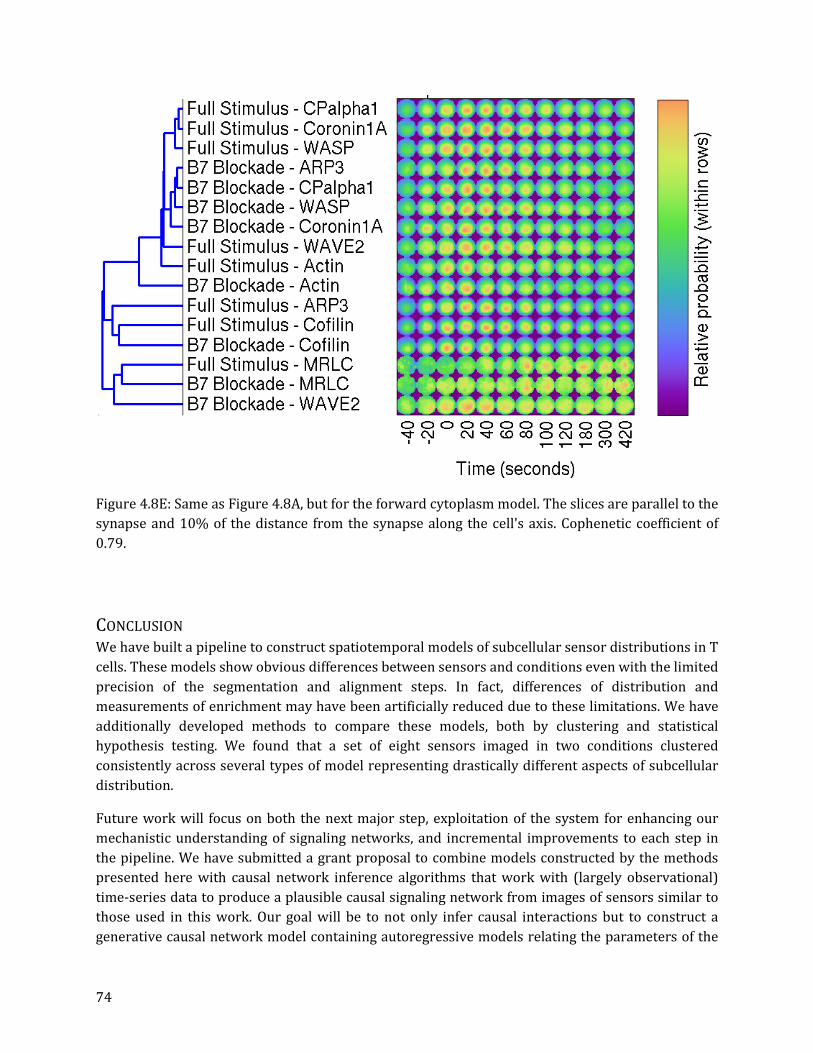
74
Figure 4.8E: Same as Figure 4.8A, but for the forward cytoplasm model. The slices are parallel to the synapse and 10% of the distance from the synapse along the cell's axis. Cophenetic coefficient of 0.79.
CONCLUSION We have built a pipeline to construct spatiotemporal models of subcellular sensor distributions in T cells. These models show obvious differences between sensors and conditions even with the limited precision of the segmentation and alignment steps. In fact, differences of distribution and measurements of enrichment may have been artificially reduced due to these limitations. We have additionally developed methods to compare these models, both by clustering and statistical hypothesis testing. We found that a set of eight sensors imaged in two conditions clustered consistently across several types of model representing drastically different aspects of subcellular distribution.
Future work will focus on both the next major step, exploitation of the system for enhancing our mechanistic understanding of signaling networks, and incremental improvements to each step in the pipeline. We have submitted a grant proposal to combine models constructed by the methods presented here with causal network inference algorithms that work with (largely observational) time-series data to produce a plausible causal signaling network from images of sensors similar to those used in this work. Our goal will be to not only infer causal interactions but to construct a generative causal network model containing autoregressive models relating the parameters of the

75
spatial distributions of signal molecules. More distant work would likely construct simulations of these molecules inside realistic cell shapes and further from higher resolution image data and search for molecular interactions that could reproduce the interactions of the spatial distributions implied by the causal network.
Improvements to the pipeline, while likely time-consuming, are likely to be straightforward. We plan to manually annotate images to objectively evaluate segmentation and alignment methods to enhance their accuracy and precision. The morphing step is computationally expensive, so we will search for more efficient algorithms. Ideally, we would be able to completely automatically segment and track T cells in movies without any manual annotation.


77
CHAPTER 5: CONCLUSION
CONTRIBUTIONS We summarize the contributions of this dissertation for each chapter.
CHAPTER 2: PROTEIN LOCALIZATION DEPENDENCE ON CELL CYCLE INFERRED FROM STATIC, ASYNCHRONOUS IMAGES
• As an initial effort towards learning a model of cell cycle-related variation in images of nuclei in an unsupervised manner, we showed that manifold learning could reconstruct temporal relationships from features representing single nuclear images. Specifically, we applied Isomap to nuclear intensity, shape, and texture features and found good correspondence (a testing adjusted R-square of 0.70) between the embedding coordinates returned by Isomap for a nuclear image and the amount of time since the last cell division for that image.
CHAPTER 3: RANDOM-WALK BASED SIMULATION OF CELL AND NUCLEAR SHAPE CHANGES • We have produced a nonparametric generative joint model of 3D nuclear and cellular shape. • We have generalized the image registration, interpolation, and distance computation
method from [69] (the simplified Christensen-Rabbit-Miller algorithm approximation to the LDDMM framework [53]) to:
o have flexible kernel size so that cells with high aspect ratio, i.e., large, flat, thin regions as in fibroblasts, can have distances computed in a reasonable amount of time;
o integrate its ODEs using any explicit Runge-Kutta integration method; and o have adaptive step size for error control and limitation of the maximum
deformation per step (the latter being part of the complete Christensen-Rabbit-Miller algorithm).
• We have demonstrated application of low-rank distance matrix completion [76] in order to reduce the computational complexity of Euclidean shape space construction to linear time.
o This will likely be useful for shape space construction with parametric shape representations for very large numbers of shapes and parameters.
o This will have to be extended to include estimators for low-rank approximations to non-Euclidean distance matrices or, more directly, estimators for positions in a shape space, as the number of degrees of freedom in a shape space is linear in the number of shapes and in the dimensionality of the shape space.
o This was use to demonstrate the non-Euclidean nature of LDDMM distance matrices.
CHAPTER 4: AUTOMATED ANALYSIS OF SPATIOTEMPORAL PATTERNING OF PROTEINS IN HELPER T CELLS DURING SYNAPSE FORMATION
• We have constructed a computational pipeline that produces five types of spatiotemporal model of subcellular protein distribution in T cells around the time of synapse formation given raw images and a single point located at the center of the synapse of each cell for each frame of a time series.

78
o We used histogram equalization to flatten intensity variations within cells to produce an image closer to white-on-black to simplify image segmentation.
o We segmented the cells using an active contour method with smoothness constraints (such constraints do not exist with traditional watershed-based methods).
o We used our improved version of LDDMM (Chapter 3) to standardize the shape of each segmented cell to a half-ellipsoid shape so that each cell had a comparable coordinate system.
o We created five models summarizing different aspects of the distribution of a sensor within the standardized shape.
o Finally, we learned the parameters of each of these spatiotemporal models from thousands of cells for each condition-sensor combination.
• We have hierarchically clustered model parameters learned for eight sensors across two conditions and shown that a set of condition-sensor combinations consistently show similar spatiotemporal distributions.
• We have automatically produced enrichment plots for each of the condition-sensor combinations and statistically tested enrichment between conditions at each time point and for each sensor. Enrichment was significantly different (𝑝 < 0.05 after correction) for multiple time points for four sensors.
FUTURE WORK We present likely and possible future work for each chapter below.
Generally, future work for each of these projects involves its application, hopefully by a large number of experimentalists and not just by us, to carefully selected data sets in order to provide insight into the changes associated with different experimental conditions. For example, while one may simply measure the rate at which cells proliferate while evaluating a particular drug, one might also perform high content screening by inferring cell cycle-related distributions for many proteins for control and treated cells and noting which ones change significantly between the two conditions. One could also build models of the shape spaces and trajectories through those shape spaces from timeseries imaging assays of migratory cell invasion and ask how conditions (drugs, oxygenation, temperature, etc.) change the behavior of the cell in terms of its shape. Given time-series images of embryonic development, one might wish to quantify changes in patterning of transcription factors under control and knockout conditions. The present and future products of all three chapters could give automatic and consistent quantification of the effects of perturbation in each of these three cases. The two major long-term goals for this work are: to increase the speed and performance of these methods such that they become indispensable tools for other researchers; and to generalize the methods so that they apply to wider classes of data. Accomplishing the latter goal will involve computer vision work to properly extract and characterize objects from images (e.g., cells of other morphologies, modeled in works such as [21, 95], or the aforementioned embryos) and model construction for the distributions of sensors within these objects.

79
CHAPTER 2: PROTEIN LOCALIZATION DEPENDENCE ON CELL CYCLE INFERRED FROM STATIC, ASYNCHRONOUS IMAGES Before further methods development, we would ideally collect ground truth in the form of a number of high-resolution videos of cells from multiple cell lines expressing a fluorescent nuclear marker, e.g., a histone–GFP fusion protein. We would then track cells over the course of these videos and mark cell divisions so that we could regress nuclear appearance onto time since the last cell division (we could also call this a continuous version of cell cycle phase). With a sufficient number of cells, we could discard all but one frame of each cell's video to create an artificial dataset that simulates having acquired only static images.
For one or several methods intended to build a model of cell cycle-related variation in nuclear appearance, we would learn parameters from features representing nuclear images in this simulated static image set. These trained models would be used to predict cell cycle phase, and the predicted phases would be compared with the ground truth phases, e.g., by correlation or R-square. We would then use the trained nuclear model to infer phase for a large set of static images that include both nuclear and randomly tagged protein channels. These inferred phases would provide the independent variable values for building regression models identifying the phase-related variation in each protein's distribution. Statistical hypothesis testing could filter the regression models to give a set of candidates for proteins that significantly change location over the cell cycle.
As further effort on this project, we have already produced a statistical model and machine learning method for a kind of manifold learning tailored to this kind of data (under certain assumptions). Latent regression analysis (LRA) [48] is a related, simpler model and associated learning algorithm where the data are assumed to come from a linear process that has a beginning and end, i.e., the data are distributed on a line segment in feature space, and have subsequently been corrupted with (usually Gaussian) noise. The probability of data appearing at a particular position on this line segment is not necessarily uniform as it can come from any beta distribution. This model can be used to fit data where the expected distribution of individuals is somewhere between a two-component mixture model and a continuous, linear process, and the fitted model's beta distribution's shape will indicate to what degree the process is in fact a mixture model by to what degree the distribution looks U-shaped (that is, the probability is concentrated at the ends of the line segment).
Our work on this project has extended LRA to use a polynomial parametric curve rather than a line segment, to use a generalized beta distribution rather than a beta distribution, and to impose a prior belief on the level of noise expected in the data. (Note that we envision this model before [48] was published.) These modifications provide several generalizations to the assumptions of LRA: that the features are possibly nonlinearly related to the process of interest; that the process may be a finite mixture of more than two groups; and that some groups may be more concentrated while others more spread out, as if part of a continuous mixture. The prior belief would hopefully also eliminate singularities, i.e., failures of the learning algorithm, to which both Gaussian mixture model and LRA fitting are prone. We implemented the learning algorithm for this polynomial extension of LRA, but we found that certain portions of the implementation will require modification so that certain values can be stably computed using floating point operations. As we ran out of funding for

80
this project before we could research and then make these modifications, we have not finished the implementation. This model could be of more general use than just for this project, perhaps for many applications where people currently fit mixture models primarily due to the lack of (knowledge of) any alternatives, so part of our future work would be to complete this implementation and use it to learn models of phase from nuclear image features.
Ultimately, the LRA model may be extendable to more than one latent variable, which could have applications in, for example, learning how the phenotype of the nucleus changes over the course of the cell cycle as a drug is applied in unknown concentrations (e.g., due to variable penetration of the drug into the environment or variation in the amount of drugs taken up by each individual cell). This could also be used to find a continuous basis for subcellular protein distributions.
An interesting outcome of having models of the cell cycle-related variation of protein distributions is that we could attempt to infer causal relationships between protein distributions. Granger causality measures the degree to which statistical predictability of one variable is affected by knowledge of the value of another variable. This is usually referred to as "Granger causality" due to it being a statistical rather than a causal measure in the general case. However, recent theoretical work has shown that under certain circumstances Granger causality is an indicator of truly causal relationships [96]. It is possible that we could use a modified form of Granger causality, which is usually applied to time-series data, with the continuous models of cell cycle-dependent protein distribution that we would produce to infer possible interactions between proteins while imaging only one a time.
CHAPTER 3: RANDOM-WALK BASED SIMULATION OF CELL AND NUCLEAR SHAPE CHANGES The next step for this work would be to derive estimators for the position of each training shape in a low-dimensional Euclidean shape space from a potentially non-Euclidean and incomplete the observed distance matrix. We know that this is possible because the output from MDS has a number of degrees of freedom linear in the number of shapes and the dimensionality of the shape space while the distance matrix's degrees of freedom increase quadratic with the number of shapes in the general case. The question is how to estimate these positions with low bias without requiring the entire distance matrix.
Afterwards, we would acquire microscopic videos of fluorescently labeled cells from which we could extract high-quality cellular and nuclear shapes; build a shape space with the reduced-complexity method so that we could feasibly use a large number of shapes; and train the nonparametric KDE-based transition model on trajectories in the shape space. We would then have a model where we could predict trajectories of shapes anywhere in the shape space. Applying this to movies of migrating cells should produce transition probabilities from migrating to stopping or turning that vary depending on the general processivity for that cell type as well as experimental conditions and thus be useful for detecting and quantifying changes in cell behavior.
Finally, the improvements in the model proposed here would be migrated to CellOrganizer and made available online.

81
CHAPTER 4: AUTOMATED ANALYSIS OF SPATIOTEMPORAL PATTERNING OF PROTEINS IN HELPER T CELLS DURING SYNAPSE FORMATION Near-future work here would improve the image processing for more accurate and precise spatiotemporal maps of sensor distributions. This will allow us to confidently model cell-to-cell variability in sensor distributions, e.g., by clustering the patterns of sensors in individual cells rather than clustering their averaged models. As a consequence, we might even discover rare or subtle patterns not found through visual inspection. The result of this would be a classification of every cell as belonging to one of these patterns, in which case we could produce tables showing the prevalence of each pattern as a function of time as in [7] and we could easily statistically compare these low-dimensional representations of distributions across sensors and across conditions.
Reliable subcellular distributions for proteins and other signaling molecules could provide negative examples of protein-protein interactions, which are difficult enough to definitively produce that protein interaction networks are based on high throughput data for only positive examples [97, 98], and negative examples are either guessed randomly (as the vast majority interactions do not occur [97]) or are sometimes hypothesized from disagreement between interaction detection methods [99]. With our maps, we would measure a linear number of maps (i.e., one for each sensor) and compare them computationally, e.g., in a pair-wise manner (or with larger tuples of proteins). This would not eliminate the combinatorial explosion of the number of tests involved, but it would eliminate the explosion of the number of experiments needed. A negative example would be detected by an extremely low probability of interaction as measured by a low intersection of the probability distributions of the proteins involved in the interaction. While a high degree of overlap between the distributions does not necessarily imply that the proteins interact, proteins that interact at a high rate, i.e., in a particular location in the cell and at a particular time relative to synapse formation, would necessarily also appear in that location and at that time in high concentrations. Therefore, very low probability density in a location at a time for at least one of a set of proteins implies that the set simultaneously directly interacts at that location and time with very low probability. We should thus be able to produce spatiotemporal maps of interactions that cannot happen with much probability, constraining the structure of the as yet unknown true interaction network with spatial and temporal resolution.
More importantly, these learned models can be used with Granger causality-based methods in order to infer significant likely causal interaction (not merely statistical predictability) between many sensors as mentioned above [96]. Ideally, this would result in a high-confidence causal network of sensors along with a model of how the spatiotemporal distribution of one sensor or the presence of a perturbation affects the distribution of another sensor. We would then validate or refute these causal interactions by manipulating causes both experimentally and through this causal network and comparing prediction with outcome.
In the more distant future, we would like to apply methods developed as above to other signaling networks within cells, between cells, between organisms, or to other similar systems.


83
REFERENCES [1] K. L. Singleton, K. T. Roybal, Y. Sun et al., “Spatiotemporal patterning during T cell activation
is highly diverse,” Sci Signal, vol. 2, no. 65, pp. ra15, 2009. [2] A. Sigal, R. Milo, A. Cohen et al., “Dynamic proteomics in individual human cells uncovers
widespread cell-cycle dependence of nuclear proteins,” Nature Methods, vol. 3, no. 7, pp. 525-31, 2006.
[3] S. Farkash-Amar, E. Eden, A. Cohen et al., “Dynamic proteomics of human protein level and localization across the cell cycle,” PloS one, vol. 7, no. 11, pp. e48722, 2012.
[4] J. Schweizer, M. Loose, M. Bonny et al., “Geometry sensing by self-organized protein patterns,” Proceedings of the National Academy of Sciences, vol. 109, no. 38, pp. 15283-15288, 2012.
[5] M. Machacek, L. Hodgson, C. Welch et al., “Coordination of Rho GTPase activities during cell protrusion,” Nature, vol. 461, no. 7260, pp. 99-103, Sep 3, 2009.
[6] R. Poincloux, O. Collin, F. Lizárraga et al., “Contractility of the cell rear drives invasion of breast tumor cells in 3D Matrigel,” Proceedings of the National Academy of Sciences, vol. 108, no. 5, pp. 1943-1948, 2011.
[7] K. L. Singleton, M. Gosh, R. D. Dandekar et al., “Itk controls the spatiotemporal organization of T cell activation,” Science signaling, vol. 4, no. 193, pp. ra66, Oct 4, 2011.
[8] T. Zhao, and R. F. Murphy, “Automated learning of generative models for subcellular location: Building blocks for systems biology,” Cytometry Part A, vol. 71A, pp. 978-990, 2007.
[9] J. Newberg, J. Hua, and R. F. Murphy, "Location proteomics: systematic determination of protein subcellular location," Systems Biology, pp. 313-332: Springer, 2009.
[10] R. F. Murphy, M. Velliste, and G. Porreca, “Robust numerical features for description and classification of subcellular location patterns in fluorescence microscope images,” Journal of VLSI signal processing systems for signal, image and video technology, vol. 35, no. 3, pp. 311-321, 2003.
[11] M. Ashburner, C. A. Ball, J. A. Blake et al., “Gene Ontology: tool for the unification of biology,” Nature genetics, vol. 25, no. 1, pp. 25-29, 2000.
[12] L. P. Coelho, T. Peng, and R. F. Murphy, “Quantifying the distribution of probes between subcellular locations using unsupervised pattern unmixing,” Bioinformatics, vol. 26, no. 12, pp. i7-i12, 2010.
[13] E. Glory, J. Newberg, and R. F. Murphy, “AUTOMATED COMPARISON OF PROTEIN SUBCELLULAR LOCATION PATTERNS BETWEEN IMAGES OF NORMAL AND CANCEROUS TISSUES,” Proc IEEE Int Symp Biomed Imaging, vol. 4540993, pp. 304-307, 2008.
[14] A. Shariff, R. F. Murphy, and G. K. Rohde, “A generative model of microtubule distributions, and indirect estimation of its parameters from fluorescence microscopy images,” Cytometry A, vol. 77, no. 5, pp. 457-66, 2010.
[15] A. Shariff, R. F. Murphy, and G. K. Rohde, “AUTOMATED ESTIMATION OF MICROTUBULE MODEL PARAMETERS FROM 3-D LIVE CELL MICROSCOPY IMAGES,” Proc IEEE Int Symp Biomed Imaging, vol. 2011, no. March 30 2011-April 2 2011, pp. 1330-1333, 2011.
[16] J. Li, A. Shariff, M. Wiking et al., “Estimating Microtubule Distributions from 2D Immunofluorescence Microscopy Images Reveals Differences among Human Cultured Cell Lines,” PloS one, vol. 7, no. 11, pp. e50292, 2012.
[17] G. K. Rohde, W. Wang, T. Peng et al., "Deformation-based nonlinear dimension reduction: Applications to nuclear morphometry." pp. 500-503.
[18] G. K. Rohde, A. J. S. Ribeiro, K. N. Dahl et al., “Deformation-based nuclear morphometry: Capturing nuclear shape variation in HeLa cells,” Cytometry Part A, vol. 73A, pp. 341-350, 2008.

84
[19] T. Peng, W. Wang, G. K. Rohde et al., “Instance-Based Generative Biological Shape Modeling,” Proc IEEE Int Symp Biomed Imaging, vol. 5193141, pp. 690-693, 2009.
[20] Z. Pincus, and J. A. Theriot, “Comparison of quantitative methods for cell-shape analysis,” J Microsc, vol. 227, no. Pt 2, pp. 140-56, 2007.
[21] T. Peng, and R. F. Murphy, “Image-derived, three-dimensional generative models of cellular organization,” Cytometry Part A, vol. 79A, pp. 383–391, 2011.
[22] C. Bakal, J. Aach, G. Church et al., “Quantitative morphological signatures define local signaling networks regulating cell morphology,” Science, vol. 316, no. 5832, pp. 1753-6, 2007.
[23] R. F. Murphy, “Communicating subcellular distributions,” Cytometry A, vol. 77, no. 7, pp. 686-92, 2010.
[24] T. E. Buck, J. Li, G. K. Rohde et al., “Toward the virtual cell: automated approaches to building models of subcellular organization "learned" from microscopy images,” Bioessays, vol. 34, no. 9, pp. 791-9, 2012.
[25] R. F. Murphy, "(3) The CellOrganizer project: An open source system to learn image-derived models of subcellular organization over time and space." pp. 1-2.
[26] I. Hepburn, W. Chen, S. Wils et al., “STEPS: efficient simulation of stochastic reaction-diffusion models in realistic morphologies,” BMC Syst Biol, vol. 6, no. 1, pp. 36, 2012.
[27] J. Czech, M. Dittrich, and J. R. Stiles, "Rapid creation, Monte Carlo simulation, and visualization of realistic 3D cell models," Systems Biology, pp. 237-287: Springer, 2009.
[28] M. J. Byrne, M. N. Waxham, and Y. Kubota, “Cellular dynamic simulator: an event driven molecular simulation environment for cellular physiology,” Neuroinformatics, vol. 8, no. 2, pp. 63-82, 2010.
[29] R. A. Kerr, T. M. Bartol, B. Kaminsky et al., “Fast Monte Carlo simulation methods for biological reaction-diffusion systems in solution and on surfaces,” SIAM Journal on Scientific Computing, vol. 30, no. 6, pp. 3126-3149, 2008.
[30] A. E. Cowan, I. I. Moraru, J. C. Schaff et al., “Spatial modeling of cell signaling networks,” Methods in cell biology, vol. 110, pp. 195, 2012.
[31] K. Lipkow, and D. J. Odde, “Model for Protein Concentration Gradients in the Cytoplasm,” Cellular and molecular bioengineering, vol. 1, no. 1, pp. 84, 2008.
[32] B. M. Regner, D. Vučinić, C. Domnisoru et al., “Anomalous Diffusion of Single Particles in Cytoplasm,” Biophysical journal, vol. 104, no. 8, pp. 1652-1660, 2013.
[33] S. Nadkarni, T. Bartol, T. Sejnowski et al., “Are the docked vesicles at CA3-CA1 synapses at the,” 2009.
[34] V. I. Maly, and I. V. Maly, “Symmetry, stability, and reversibility properties of idealized confined microtubule cytoskeletons,” Biophys J, vol. 99, no. 9, pp. 2831-40, 2010.
[35] S. Nadkarni, T. M. Bartol, T. J. Sejnowski et al., “Modelling vesicular release at hippocampal synapses,” PLoS Comput Biol, vol. 6, no. 11, pp. e1000983, 2010.
[36] C. H. Schreiber, M. Stewart, and T. Duke, “Simulation of cell motility that reproduces the force-velocity relationship,” Proc Natl Acad Sci U S A, vol. 107, no. 20, pp. 9141-6, 2010.
[37] L. Wang, C. E. Castro, and M. C. Boyce, “Growth strain-induced wrinkled membrane morphology of white blood cells,” Soft Matter, vol. 7, pp. 11319-11324, 2011.
[38] C. I. Lacayo, Z. Pincus, M. M. VanDuijn et al., “Emergence of large-scale cell morphology and movement from local actin filament growth dynamics,” PLoS Biol, vol. 5, no. 9, pp. e233, 2007.
[39] E. Atilgan, D. Wirtz, and S. X. Sun, “Morphology of the lamellipodium and organization of actin filaments at the leading edge of crawling cells,” Biophysical journal, vol. 89, no. 5, pp. 3589-3602, 2005.
[40] Y. Hu, E. Osuna-Highley, J. Hua et al., “Automated analysis of protein subcellular location in time series images,” Bioinformatics, vol. 26, no. 13, pp. 1630-1636, 2010.

85
[41] T. E. Buck, A. Rao, L. P. Coelho et al., “Cell cycle dependence of protein subcellular location inferred from static, asynchronous images,” Conf Proc IEEE Eng Med Biol Soc, vol. 2009, pp. 1016-9, 2009.
[42] L. Barbe, E. Lundberg, P. Oksvold et al., “Toward a confocal subcellular atlas of the human proteome,” Mol Cell Proteomics, vol. 7, no. 3, pp. 499-508, 2008.
[43] K. T. Roybal, P. Sinai, P. Verkade et al., “The actin-driven spatiotemporal organization of signaling in T cells activated by antigen presenting cells,” Immunological Reviews, vol. In press, 2013.
[44] K. Keren, Z. Pincus, G. M. Allen et al., “Mechanism of shape determination in motile cells,” Nature, vol. 453, no. 7194, pp. 475-80, 2008.
[45] T. E. Buck, A. Rao, L. P. Coelho et al., "Cell cycle dependence of protein subcellular location inferred from static, asynchronous images." pp. 1016-9.
[46] X. Zhou, F. Li, J. Yan et al., “A Novel Cell Segmentation Method and Cell Phase Identification Using Markov Model,” IEEE Transactions on Information Technology in Biomedicine, vol. 13, no. 2, pp. 152-7, 2009.
[47] T. E. Buck, J. Li, G. K. Rohde et al., “Toward the virtual cell: Automated approaches to building models of subcellular organization “learned” from microscopy images,” BioEssays, 2012.
[48] T. Tarpey, and E. Petkova, “Latent regression analysis,” Statistical Modelling, vol. 10, no. 2, pp. 133-58, 2010.
[49] B. Schölkopf, A. Smola, and K.-R. Müller, "Kernel principal component analysis," Advances in kernel methods pp. 327-52, Cambridge, MA, USA: MIT Press, 1999.
[50] J. B. Tenenbaum, V. d. Silva, and J. C. Langford, “A Global Geometric Framework for Nonlinear Dimensionality Reduction,” Science vol. 290, no. 5500, pp. 2319-2323, 2000.
[51] S. T. Roweis, and L. K. Saul, “Nonlinear Dimensionality Reduction by Locally Linear Embedding,” Science, vol. 290, no. 5500, pp. 2323-2326, 2000.
[52] M. Belkin, and P. Niyogi, “Laplacian eigenmaps for dimensionality reduction and data,” Neural Computation, vol. 15, no. 6, pp. 1373-96, 2003.
[53] M. F. Beg, M. I. Miller, A. Trouvé et al., “Computing large deformation metric mappings via geodesic flows of diffeomorphisms,” International journal of computer vision, vol. 61, no. 2, pp. 139-157, 2005.
[54] K. L. Singleton, K. T. Roybal, Y. Sun et al., “Spatiotemporal Patterning During T Cell Activation Is Highly Diverse,” Science Signaling, vol. 2, no. 65, pp. ra15, April, 2009.
[55] B. H. Cho, C. Wülfing, and R. F. Murphy, "Automated identification of subcellular patterns of T cell signaling proteins," 2013, in preparation.
[56] B. B. Avants, N. Tustison, and G. Song, “Advanced Normalization Tools (ANTS),” Insight J, 2009.
[57] J. Ashburner, “A fast diffeomorphic image registration algorithm,” Neuroimage, vol. 38, no. 1, pp. 95-113, 2007.
[58] B. B. Avants, P. Yushkevich, J. Pluta et al., “The optimal template effect in hippocampus studies of diseased populations,” Neuroimage, vol. 49, no. 3, pp. 2457-2466, 2010.
[59] S. Klöppel, C. M. Stonnington, C. Chu et al., “Automatic classification of MR scans in Alzheimer's disease,” Brain, vol. 131, no. 3, pp. 681-689, 2008.
[60] K. Oishi, S. Mori, P. K. Donohue et al., “Multi-contrast human neonatal brain atlas: application to normal neonate development analysis,” NeuroImage, vol. 56, no. 1, pp. 8-20, 2011.
[61] M. V. Boland, and R. F. Murphy, “A neural network classifier capable of recognizing the patterns of all major subcellular structures in fluorescence microscope images of HeLa cells,” Bioinformatics, vol. 17, no. 12, pp. 1213-23, 2001.

86
[62] M. Gooden, R. Vernon, J. Bassuk et al., “Cell cycle-dependent nuclear location of the matricellular protein SPARC: Association with the nuclear matrix,” Journal of cellular biochemistry, vol. 74, no. 2, pp. 152-167, 1999.
[63] M. Miura, H. Watanabe, T. Sasaki et al., “Dynamic changes in subnuclear NP95 location during the cell cycle and its spatial relationship with DNA replication foci,” Experimental cell research, vol. 263, no. 2, pp. 202-208, 2001.
[64] E. G. Osuna, J. Hua, N. W. Bateman et al., “Large-scale automated analysis of location patterns in randomly tagged 3T3 cells,” Annals of biomedical engineering, vol. 35, no. 6, pp. 1081-1087, 2007.
[65] J. Jarvik, S. Adler, C. Telmer et al., “CD-tagging: a new approach to gene and protein discovery and analysis,” Biotechniques, vol. 20, no. 5, pp. 896-904, 1996.
[66] J. B. Tenenbaum, V. d. Silva, and J. C. Langford, “A Global Geometric Framework for Nonlinear Dimensionality Reduction,” Science, vol. 290, no. 5500, pp. 2319-2323, 2000.
[67] N. Mekuz, and J. K. Tsotsos, "Parameterless Isomap with adaptive neighborhood selection," Pattern Recognition, pp. 364-373: Springer, 2006.
[68] Y. Bengio, J.-F. Paiement, and P. Vincent, "Out-of-sample extensions for lle, isomap, mds, eigenmaps, and spectral clustering." pp. 177-184.
[69] T. Peng, W. Wang, G. K. Rohde et al., "Instance-based generative biological shape modeling." pp. 690-693.
[70] C. C. Fink, B. Slepchenko, I. I. Moraru et al., “Morphological control of inositol-1, 4, 5-trisphosphate–dependent signals,” The Journal of cell biology, vol. 147, no. 5, pp. 929-936, 1999.
[71] G. E. Christensen, R. D. Rabbitt, and M. I. Miller, “Deformable templates using large deformation kinematics,” Image Processing, IEEE Transactions on, vol. 5, no. 10, pp. 1435-1447, 1996.
[72] M. Velliste, and R. F. Murphy, "Automated determination of protein subcellular locations from 3D fluorescence microscope images." pp. 867-870.
[73] A. Shariff, R. F. Murphy, and G. K. Rohde, "Automated estimation of microtubule model parameters from 3-d live cell microscopy images." pp. 1330-1333.
[74] T. F. Chan, and L. A. Vese, “Active contours without edges,” Image Processing, IEEE Transactions on, vol. 10, no. 2, pp. 266-277, 2001.
[75] P. Bogacki, and L. F. Shampine, “A 3 (2) pair of Runge-Kutta formulas,” Applied Mathematics Letters, vol. 2, no. 4, pp. 321-325, 1989.
[76] P. Drineas, A. Javed, M. Magdon-Ismail et al., "Distance matrix reconstruction from incomplete distance information for sensor network localization." pp. 536-544.
[77] B. Mishra, G. Meyer, and R. Sepulchre, "Low-rank optimization for distance matrix completion." pp. 4455-4460.
[78] R. F. Murphy, M. V. Boland, and M. Velliste, "Towards a Systematics for Protein Subcellular Location: Quantitative Description of Protein Localization Patterns and Automated Analysis of Fluorescence Microscope Images." pp. 251-259.
[79] M.-C. Hung, and W. Link, “Protein localization in disease and therapy,” Journal of Cell Science, vol. 124, no. 20, pp. 3381-3392, 2011.
[80] A. Bairoch, R. Apweiler, C. H. Wu et al., “The universal protein resource (UniProt),” Nucleic acids research, vol. 33, no. suppl 1, pp. D154-D159, 2005.
[81] M. Uhlen, P. Oksvold, L. Fagerberg et al., “Towards a knowledge-based human protein atlas,” Nature biotechnology, vol. 28, no. 12, pp. 1248-1250, 2010.
[82] M. V. Boland, and R. F. Murphy, “A neural network classifier capable of recognizing the patterns of all major subcellular structures in fluorescence microscope images of HeLa cells,” Bioinformatics, vol. 17, no. 12, pp. 1213-1223, 2001.

87
[83] K. Huang, and R. Murphy, “Boosting accuracy of automated classification of fluorescence microscope images for location proteomics,” Bmc Bioinformatics, vol. 5, no. 1, pp. 78, 2004.
[84] J. Li, J. Y. Newberg, M. Uhlén et al., “Automated analysis and reannotation of subcellular locations in confocal images from the human protein atlas,” PloS one, vol. 7, no. 11, pp. e50514, 2012.
[85] K. L. Singleton, N. Parvaze, K. R. Dama et al., “A large T cell invagination with CD2 enrichment resets receptor engagement in the immunological synapse,” J. Immunol., vol. 177, no. 7, pp. 4402-13, 2006.
[86] C. R. Monks, B. A. Freiberg, H. Kupfer et al., “Three-dimensional segregation of supramolecular activation clusters in T cells,” Nature, vol. 395, no. 6697, pp. 82-86, 1998.
[87] I. Tskvitaria-Fuller, N. Mistry, S. Sun et al., “Protein transduction as a means of effective manipulation of Cdc42 activity in primary T cells,” J Immunol Methods, vol. 319, no. 1-2, pp. 64-78, Jan 30, 2007.
[88] Y. Sun, R. D. Dandekar, Y. S. Mao et al., “Phosphatidylinositol (4,5) bisphosphate controls T cell activation by regulating T cell rigidity and organziation,” PLoS ONE, vol. 6, pp. e27227, 2011.
[89] D.-J. Kroon, C. H. Slump, and T. J. Maal, "Optimized anisotropic rotational invariant diffusion scheme on cone-beam CT," Medical Image Computing and Computer-Assisted Intervention–MICCAI 2010, pp. 221-228: Springer, 2010.
[90] H. Scharr, "Optimal filters for extended optical flow," Complex Motion, pp. 14-29: Springer, 2007.
[91] M. Kass, A. Witkin, and D. Terzopoulos, “Snakes: Active contour models,” International journal of computer vision, vol. 1, no. 4, pp. 321-331, 1988.
[92] C. Lürig, L. Kobbelt, and T. Ertl, “Hierarchical solutions for the deformable surface problem in visualization,” Graphical Models, vol. 62, no. 1, pp. 2-18, 2000.
[93] B. L. Welch, “The generalization ofstudent's' problem when several different population variances are involved,” Biometrika, vol. 34, no. 1/2, pp. 28-35, 1947.
[94] S. Holm, “A simple sequentially rejective multiple test procedure,” Scandinavian journal of statistics, pp. 65-70, 1979.
[95] T. Zhao, and R. F. Murphy, “Automated learning of generative models for subcellular location: building blocks for systems biology,” Cytometry A, vol. 71, no. 12, pp. 978-90, 2007.
[96] H. White, K. Chalak, and X. Lu, “Linking Granger Causality and the Pearl Causal Model with Settable Systems,” Journal of Machine Learning Research-Proceedings Track, vol. 12, pp. 1-29, 2011.
[97] M. Thahir, T. Sharma, and M. Ganapathiraju, "An efficient heuristic method for active feature acquisition and its application to protein-protein interaction prediction." p. S2.
[98] L. G. Trabuco, M. J. Betts, and R. B. Russell, “Negative protein-protein interaction datasets derived from large-scale two-hybrid experiments,” Methods, 2012.
[99] J. S. Bader, A. Chaudhuri, J. M. Rothberg et al., “Gaining confidence in high-throughput protein interaction networks,” Nat Biotech, vol. 22, no. 1, pp. 78-85, 01//print, 2004.