assessment of climate change impacts on the hydrology of ... · assessment of climate change...
TRANSCRIPT

Assessment of Climate Change Impacts on the Hydrology of Gilgel Abbay Catchment in Lake
Tana Basin, Ethiopia
Abdo Kedir Shaka
March, 2008

Assessment of Climate Change Impacts on the Hydrology of Gilgel Abbay Catchment in Lake Tana
Basin, Ethiopia
by
Abdo Kedir
Thesis submitted to the International Institute for Geo-information Science and Earth Observation in
partial fulfilment of the requirements for the degree of Master of Science in Geo-information Science
and Earth Observation, Specialisation: Integrated Watershed Modelling and Management
Thesis Assessment Board
Prof. Dr. Z. Bob Su (chairman) Head WRS dept, ITC Enschede
Dr. M. McCartney (external examiner) IWMI, East Africa office
Dr.Ing. T.H.M. Rientjes (first supervisor) WRS dept, ITC, Enschede
Dr. A.S.M. Gieske (second supervisor) WRS dept., ITC, Enschede
INTERNATIONAL INSTITUTE FOR GEO-INFORMATION SCIENCE AND EARTH OBSERVATION
ENSCHEDE, THE NETHERLANDS

Disclaimer This document describes work undertaken as part of a programme of study at the International Institute for Geo-information Science and Earth Observation. All views and opinions expressed therein remain the sole responsibility of the author, and do not necessarily represent those of the institute.

DedicateDedicateDedicateDedicatedddd to my to my to my to my mo mo mo motherthertherther Lubaba Aman Lubaba Aman Lubaba Aman Lubaba Aman MomMomMomMom,,,, you are you are you are you are the main reason the main reason the main reason the main reason for for for for being what I am being what I am being what I am being what I am

i
Abstract
Climate scenarios differ substantially due to uncertainties with regard to climate forcing caused by
greenhouse emissions, uncertainties caused by imperfect representation of the process in the models
and uncertainties with regard to initial condition. The General Circulation Models (GCMs) which are
considered as the most advance tools for estimating future climate change scenarios operate on a
coarse scale. However, the climate impact studies in hydrology often require climate change
information at fine spatial scale. Therefore the output from a GCM has to be downscaled to obtain
information relevant to hydrological studies.
This report presents the results of a study on downscaling large scale atmospheric variables simulated
with General Circulation Models (GCMs) to meteorological variables at local scale in order to
investigate the hydrological impact of possible future climate change in Gilgel Abbay catchment
(Ethiopia). Statistical DownScaling Model (SDSM) was employed to convert the GCM output into
daily meteorological variables appropriate for hydrological impact studies. The meteorological
variables (minimum temperature, maximum temperature and precipitation) downscaled from SDSM
were used as input to the HBV hydrological model which was calibrated (R2=0.86) and validated
(R2=0.76) with historical data to investigate the possible impact of climate change in the catchment.
The results obtained from this investigation indicate that there is significant variation in the seasonal
and monthly flow. In the main rainy season (June-September) the runoff will be reduced by 12% in
the 2080s. The result from synthetic (incremental) scenario also indicates that the catchment is
sensitive to climate change. As much as 33% of the seasonal and annual runoff will be reduced if an
increment of 2oC in temperature and reduction of 20% rainfall occur simultaneously in the catchment.
Key words Climate change, GCM, HBV, SDSM

ii
Acknowledgements
First of all I thank the almighty ALLAH for His endless Grace and Blessing on me during all these
months here at ITC and in all my life.
I would like to express my thanks and gratitude to the Directorate of ITC for granting me this
opportunity to study for a Master of Science degree. I am also grateful to my employer, South Water
Resources Development bureau for providing me leave during my study.
Very special thanks to my first supervisor, Dr.Ing.Tom Rientjes and second supervisor, Dr. Ambro
Gieske for their support and encouragement during all the course of my study. Their critical
comments and valuable advices helped me to take this research in the right directions.
I would like to thanks Dr. M. McCartney and Dr.Yasir Mohamed from IWMI for their valuable
comment in my work.
I would like to thanks also Ethiopian Ministry of Water Resources and National Meteorological
Agency for providing hydrological and meteorological data for my study.
I would like to express my appreciation to all my course mates for their support and wonderful social
atmosphere.
Back home, I wish to express my deep gratitude to all friends and family members. Their prayers for
me were the main source of inspiration, motivation and encouragement to continue this work. Special
thanks to my sister, Siti Shifa.
Last of all, thanks to everyone who helped me and I wish all of you wonderful happy days.
Abdo Kedir
March 2007

iii
Table of contents
Abstract....................................................................................................................................i Acknowledgements.................................................................................................................ii List of figures..........................................................................................................................v List of tables .........................................................................................................................vii
1. INTRODUCTION.............................................................................................................1 1.1. Background ................................................................................................................1 1.2. Research objective and question ................................................................................2 1.3. Thesis layout ..............................................................................................................3
2. STUDY AREA AND DATA AVAILABILITY...............................................................5 2.1. Study area...................................................................................................................5
2.1.1. Location .......................................................................................................................5 2.1.2. Topography ..................................................................................................................6 2.1.3. Climate.........................................................................................................................6 2.1.4. Drainage Network........................................................................................................9 2.1.5. Soil, geology and land cover......................................................................................10
2.2. Data availability .......................................................................................................10 2.2.1. Meteorological data ...................................................................................................10 2.2.2. Hydrological data.......................................................................................................12 2.2.3. Remote sensing data ..................................................................................................12 2.2.4. Climate scenario data.................................................................................................12
3. LITERATURE REVIEW................................................................................................13 3.1. Climate model ..........................................................................................................13
3.1.1. The Climatological baseline ......................................................................................14 3.1.2. Climate Scenario........................................................................................................15 3.1.3. Source of GCM and Emission Scenario ....................................................................18
3.2. Downscaling methods and tools...............................................................................20 3.2.1. Dynamic downscaling................................................................................................21 3.2.2. Empirical (statistical) downscaling............................................................................21
3.3. Hydrological model..................................................................................................23 3.3.1. Use of hydrological modelling in climate change impact studies .............................23 3.3.2. Short description of the HBV model .........................................................................24
4. METHODOLOGY..........................................................................................................29 4.1. General Circulation Model (GCM)..........................................................................29 4.2. Statistical DownScaling Model................................................................................30
4.2.1. General description of the model...............................................................................30 4.2.2. Model setup................................................................................................................33
4.3. HBV-96....................................................................................................................37 4.3.1. General description ....................................................................................................37 4.3.2. Model input................................................................................................................37
iv
4.3.3. Calibration, validation and evaluation ...................................................................... 41 4.4. Hydrological impact of climate change....................................................................44
5. RESULTS AND DISCUSSION......................................................................................47 5.1. Downscaling the GCM output..................................................................................47
5.1.1. Downscaling the GCM for the baseline period......................................................... 47 5.1.2. Downscaling the GCM for future scenario...............................................................51
5.2. Hydrological model calibration and validation results.............................................56 5.3. Hydrological impact of future climate change scenario ...........................................59 5.4. Uncertainties and sensitivity analysis.......................................................................61
6. CONCLUSION AND RECOMMENDATION...............................................................65 6.1. Conclusion................................................................................................................65 6.2. Recommendation......................................................................................................66
REFERENCE........................................................................................................................69 ANNEX.................................................................................................................................71
Annex A Definition of common terms and acronymys...................................................71 Annex B Elevation and vegetation zone of the subbasins...............................................72
v
List of figures
Figure 2.1: Location of Gilgel Abbay catchment.....................................................................................5 Figure 2.2: Slope map of Gilgel Abbay catchment..................................................................................6 Figure 2.3: Mean annual rainfall from 1996-2004...................................................................................7 Figure 2.4: Mean monthly rainfall distribution (1996-2004) for various stations in study area .............8 Figure 2.5: Mean monthly temperature from 1996-2004.........................................................................9 Figure 2.6: Flow record of Gilgel Abbay at Merawi (1997-2005) ........................................................10 Figure 2.7: Meteorological and gauging station ....................................................................................11 Figure 3.1: Schematic view of the processes and interaction in the global climate system (based on
Hadley Centre for Climate Prediction and Research)..........................................................13 Figure 3.2: Some alternative data sources and procedures for constructing climate scenarios for use in
impact assessment. Highlighted boxes indicate the baseline climate and common types of
scenario. Grey shading encloses the typical component of climate scenario generators
(Houghton, 2001) .................................................................................................................17 Figure 3.3: The four IPCC SRES scenario storylines (Carter, 2007) ....................................................20 Figure 3.4: Schematic structure of HBV-96 model................................................................................25 Figure 4.1: A schematic illustrating the general approach to downscaling (Dawson & Wilby, 2007) .30 Figure 4.2: SDSM Version 4.1 climate scenario generation (Dawson & Wilby, 2007)........................32 Figure 4.3: The Africa Continent window with 2.5° latitude x 3.75 longitude grid size and location of
the study area in the grid box. ..............................................................................................33 Figure 4.4: Steps in DEM hydroprocessing ...........................................................................................38 Figure 4.5: DEM of the Gilgel Abbay....................................................................................................39 Figure 4.6: Relationship between parameter in soil routine (SMHI, 2006)...........................................42 Figure 4.7: The response routine............................................................................................................43 Figure 4.8: Conceptual framework.........................................................................................................45 Figure 5.1: Observed and downscaled monthly mean minimum temperature for the baseline period
(1961- 1990).........................................................................................................................47 Figure 5.2: Absolute model error in estimate of monthly minimum temperature .................................48 Figure 5.3: Variance of observed and downscaled monthly minimum temperature .............................48 Figure 5.4: Observed and downscaled monthly mean maximum temperature for the baseline period
(1961-1990)..........................................................................................................................49 Figure 5.5: Absolute model error in estimate of monthly maximum temperature.................................49 Figure 5.6: Variance of observed and downscaled monthly maximum temperature.............................50 Figure 5.7: Mean daily observed and downscaled precipitation for the baseline period (1960-1990)..50 Figure 5.8: Absolute model error in estimates of the mean daily precipitation.....................................51 Figure 5.9: Variance of observed and downscaled monthly mean precipitation ...................................51 Figure 5.10: Change of downscaled monthly minimum temperature from the baseline period for
HadCM3A2a ........................................................................................................................52 Figure 5.11: Change of downscaled monthly minimum temperature from the baseline period for
HadCM3B2a......................................................................................................................52 Figure 5.12: Change in monthly maximum temperature between the baseline period and future for
HadCM3A2a......................................................................................................................53

vi
Figure 5.13: Change in monthly maximum temperature between the baseline period and future for.. 53 Figure 5.14: Mean daily precipitation downscaled from HadCM3A2a................................................ 54 Figure 5.15: Mean daily precipitation downscaled from HadCM3B2a................................................ 54 Figure 5.16: Mean daily precipitation for Ethiopian highland between the present and future ........... 55 Figure 5.17: Daily observed and simulated hydrograph during calibration period .............................. 57 Figure 5.18: Observed and simulated mean monthly hydrograph during calibration period................ 58 Figure 5.19: Daily observed and simulated hydrograph during the model development period (1996-
2005) ................................................................................................................................. 58 Figure 5.20: Mean monthly flow for A2 scenario................................................................................. 60 Figure 5.21: Mean monthly flow for B2 scenario................................................................................. 60 Figure 5.22: Comparison of change in monthly runoff between the baseline period and 2080s.......... 61

vii
List of tables
Table 2.1: List of station name, location and meteorological variables ................................................11 Table 3.1: Coupled Atmospheric General Circulation Models for which climate change simulations
held by the IPCC Data Distribution Centre (Carter, 2007).................................................18 Table 3.2: The SRES Emission Scenarios (Houghton, 2001)................................................................19 Table 4.1: Types of predictor variables .................................................................................................34 Table 4.2: Correlation matrix.................................................................................................................35 Table 4.3: Large scale predictor variables selected for SDSM..............................................................36 Table 4.4: Weight of meteorological station by the inverse distance method .......................................39 Table 4.5: Weight of meteorological station by the Thiessen polygon method ....................................40 Table 4.6: Long term potential evapotranspiration for BahirDar meteorological station (1996-2005).41 Table 4.7: Long term potential evapotranspiration for Dangila meteorological station (1996-2005)...41 Table 5.1: List of optimum parameter set in calibration........................................................................56 Table 5.2: List of objective function and its value obtained during calibration ....................................57 Table 5.3: Average increase/decrease of runoff (%) from the present condition ..................................59 Table 5.4: Annual and seasonal runoff change in percentage from incremental scenario ....................62

viii

ASSESSMENT OF CLIMATE CHANGE IMPACTS ON THE HYDROLOGY OF GILGEL ABBAY CATCHMENT IN LAKE TANA BASIN, ETHIOPIA
1
1. INTRODUCTION
1.1. Background
Climate changes refers to a change in the state of the climate that can be identified by changes in the
mean and/or the variability of its properties and that persists for an extended period, typically decade
or more. Climate change may be due to internal processes and /or external forcings. Some external
influences, such as changes in solar radiation and volcanism, occur naturally and contribute to the
natural variability of the climate system. Other external changes, such as the change in the
composition of the atmosphere that began with the industrial revolution, are the result of human
activity.
The temperature of the Earth is determined by the balance between the incoming solar radiation and
the outgoing terrestrial radiation energy. The energy coming in from the sun can pass through
atmosphere and therefore heats the surface of the Earth. But the radiation emitted from the surface of
the Earth is partly absorbed by some gases in the atmosphere, and some of it re-emitted downwards.
The effect of this is to warm the surface of the Earth and the lower part of the atmosphere. Without
this natural greenhouse effect, the temperature of the Earth would be about 30ºC cooler than it is, and
it would not be habitable. However, this important function of the atmosphere is being threatened by
the rapidly increasing concentrations of greenhouse gases well above the natural level while also new
greenhouse gases such as CFCs and the CFC replacement is added to the atmosphere as a result of
human activities (for example, CO2 from fossil-fuel burning). This will add further warming which
could threaten sustainability of the Earth (Jenkins, 2005).
Nowadays there is strong scientific evidence that indicates the average temperature of the Earth’s
surface is increasing due to greenhouse gas emissions. For instance, the average global temperature
has increased by about 0.6ºC since the late 19th century. Also the latest IPCC (Intergovernmental
Panel on Climate Change) scenarios project temperature rises of 1.4-5.8ºC, and sea level rises of 9-99
cm by 2100 (Houghton, 2001). Warming and precipitation are expected to vary considerably from
region to region. Changes in climate average and the changes in frequency and intensity of extreme
weather events are likely to have major impact on natural and human systems (Aerts & Droogers,
2004).
With respect to hydrology, climate change can cause significant impacts on water resources by
resulting changes in the hydrological cycle. For instance, the changes on temperature and precipitation
can have a direct consequence on the quantity of evapotranspiration and on both quality and quantity
of the runoff component. Consequently, the spatial and temporal availability of water resource, or in
general the water balance, can be significantly affected which in turn affects agriculture, industry and
urban development.

ASSESSMENT OF CLIMATE CHANGE IMPACTS ON THE HYDROLOGY OF GILGEL ABBAY CATCHMENT IN LAKE TANA BASIN, ETHIOPIA
2
Climate change is expected to have adverse impacts on socioeconomic development in all nations
although the degree of the impact will differ. The IPCC findings indicate that developing countries
such as Ethiopia will be more vulnerable to climate change. Climate Change may have far reaching
implications for Ethiopia due to various reasons. The economy of the country mainly depends on
agriculture, which is very sensitive to climate variations. A large part of the country is arid and
semiarid and is highly prone to desertification and drought. The country has also a fragile highland
ecosystem which is currently under stress due to population pressure. Forest, water and biodiversity
resources of the country are also climate sensitive. Climate change is therefore a case for concern
(NMSA, 2001).
Despite the fact that the impact of climate change is forecasted at the global scale, the type and
magnitude of the impact at a catchment scale is not investigated in most part of the world. Therefore it
is necessary to study the effect of climate change at this scale in order to take the effect into account
by the policy and decision makers when planning water resources management.
1.2. Research objective and question
The general objective of this study is to assess the impact of climate change on the hydrology of the
Gilgel Abbay catchment.
The specific objectives of this study are:
• to develop a better understanding of hydrological impact of climate change on the Gilgel
Abbay catchment;
• to develop and evaluate climate scenario data for maximum temperature, minimum
temperature and precipitation based on a General Circulation Model and a Statistical
DownScaling Model for Gilgel Abbay catchment;
• to develop incremental scenarios to assess the sensitivity of the catchment to climate;
• to quantify possible effects of climate change on the hydrology of Gilgel Abbay catchment
based on the downscaled climate scenario data using selected hydrological model.
In order to meet the above objectives, the research questions for this study are:
• what are the possibilities and limitations of a selected General Circulation Model and
Statistical Downscaling Model for the hydrological assessment at the catchment scale;
• what are general trends of maximum temperature, minimum temperature and precipitation
scenario in the future compared to the present condition and how this is reflected on the
hydrology of the Gilgel Abbay River.

ASSESSMENT OF CLIMATE CHANGE IMPACTS ON THE HYDROLOGY OF GILGEL ABBAY CATCHMENT IN LAKE TANA BASIN, ETHIOPIA
3
1.3. Thesis layout
This thesis comprises six chapters and is organized as follows: Chapter one is an introduction to the
study. Chapter two describes the study area and availability of data. Chapter three reports on a
literature review about the subject matter. Chapter four describes the methodology applied in this
research. In chapter five the results are shown and discussed. Chapter six finalizes the thesis by
conclusions and recommendations.

ASSESSMENT OF CLIMATE CHANGE IMPACTS ON THE HYDROLOGY OF GILGEL ABBAY CATCHMENT IN LAKE TANA BASIN, ETHIOPIA
4
ASSESSMENT OF CLIMATE CHANGE IMPACTS ON THE HYDROLOGY OF GILGEL ABBAY CATCHMENT IN LAKE TANA BASIN, ETHIOPIA
5
2. STUDY AREA AND DATA AVAILABILITY
2.1. Study area
2.1.1. Location
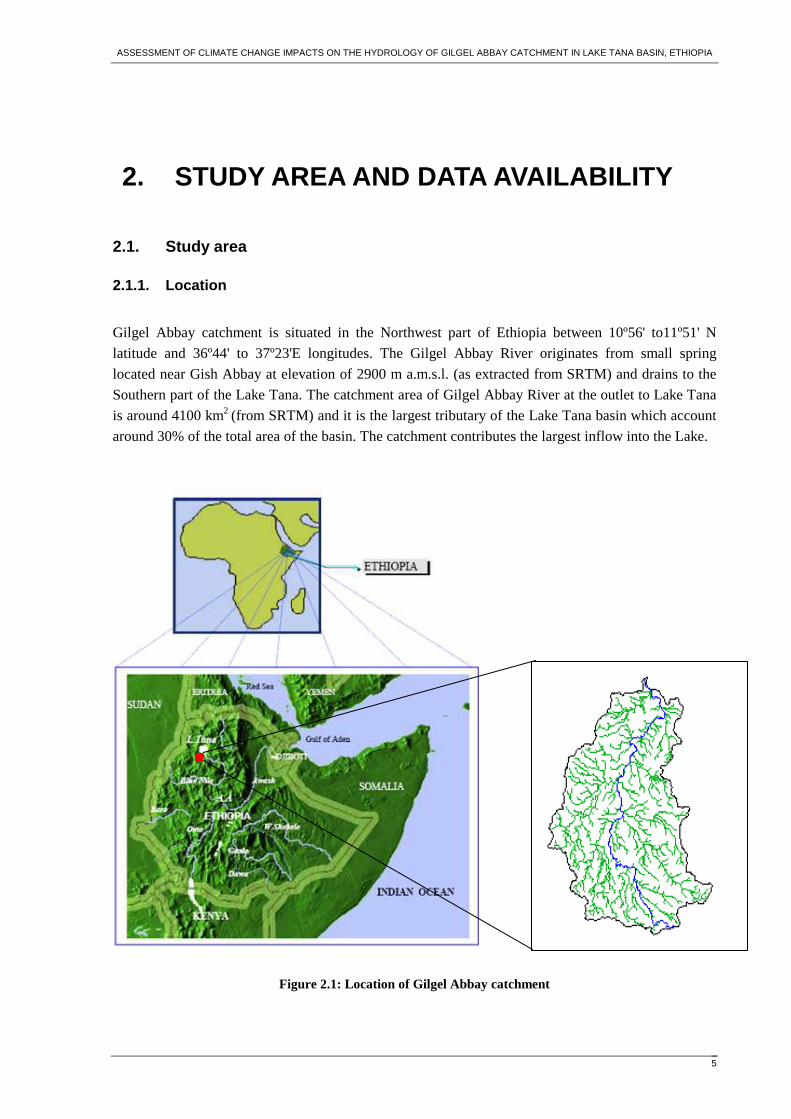
Gilgel Abbay catchment is situated in the Northwest part of Ethiopia between 10º56' to11º51' N
latitude and 36º44' to 37º23'E longitudes. The Gilgel Abbay River originates from small spring
located near Gish Abbay at elevation of 2900 m a.m.s.l. (as extracted from SRTM) and drains to the
Southern part of the Lake Tana. The catchment area of Gilgel Abbay River at the outlet to Lake Tana
is around 4100 km2 (from SRTM) and it is the largest tributary of the Lake Tana basin which account
around 30% of the total area of the basin. The catchment contributes the largest inflow into the Lake.
Figure 2.1: Location of Gilgel Abbay catchment

ASSESSMENT OF CLIMATE CHANGE IMPACTS ON THE HYDROLOGY OF GILGEL ABBAY CATCHMENT IN LAKE TANA BASIN, ETHIOPIA
6
2.1.2. Topography
The elevation of Gilgel Abbay catchment varies from 1787 to 3518m a.m.s.l. (SRTM). The higher
elevation ranges are located at the Southeast corner while the remaining area is relatively uniform.
From the slope map of the catchment area, around 70% of the catchment area falls in the slope range
from 0-8% and 25% of the area falls in the slope range of 8-30%. The remaining 5% of the area has
slope greater than 30%. The longest flow path of the river towards the outlet is 163.2 km.
Figure 2.2: Slope map of Gilgel Abbay catchment
2.1.3. Climate
The climate of Ethiopia is mainly controlled by seasonal migration of Intertropical Convergence Zone
(ITCZ) and its associated atmospheric circulation but the topography has also an effect on the local
climate. The traditional climate classification of the country is based on altitude and temperature
shows the presence of five climatic zones namely: Wurch (cold climate at more than 3000 m altitude),
Dega (temperate like climate-highland with 2500-3000 m altitude), Woina Dega ( warm-1500-2500 m
altitude), Kola (hot and arid type, less than 1500 m in altitude), and Berha (hot and hyper-arid type)
climate (NMSA, 2001). According to this classification, the majority part of the study area falls in
Woina Dega climate however, small part of study area that is mainly at the South tips of the
catchment falls in Dega Zone. There is high spatial and temporal variation of rainfall in the study area.

ASSESSMENT OF CLIMATE CHANGE IMPACTS ON THE HYDROLOGY OF GILGEL ABBAY CATCHMENT IN LAKE TANA BASIN, ETHIOPIA
7
The main rainfall season which accounts around 70-90% of the annual rainfall occurs from June to
September. Small rains also occur sporadically during February/March to May.
The mean annual rainfall (1996-2004) of the study area as shown in Figure 2.3 varies from around
1200 mm (Abbay Shelko) up to 2400 mm for Enjebara which is just outside the catchment boundary.
The mean annual rainfall (1996-2004) of Sekela station which is located around the source of Gilgel
Abbay River is around 1900 mm.
0
500
1000
1500
2000
2500
3000
Abbay
shelk
oAde
t
Bahir
Dar
Dangil
a
Enjeba
ra
Gundil
Kidam
aja
Sekela
Zege
Station name
Rai
nfal
l (m
m)
Figure 2.3: Mean annual rainfall from 1996-2004
The monthly rainfall distributions of the study area indicate that July and August are the wettest
month of the year which gets monthly rainfall amounts larger than 350 mm. The mean monthly
rainfall for Abbay shelko, BahirDar, Dangila and Sekela for the period of 1996-2004 is shown in
Figure 2.4.
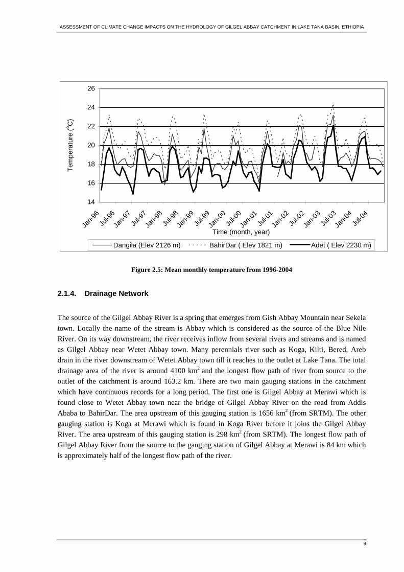
In the study area there is high diurnal change in temperature i.e. there is high variation between the
daily maximum and minimum temperature. However, the seasonal variation of temperature is less
compared to diurnal change. Generally the temperature of the area is highly affected by altitude where
the temperature decreases with increases in altitude. The mean monthly temperature of Dangila,
BahirDar and Adet meteorological stations from 1996-2004 is plotted in Figure 2.5 and this figure
indicates that the mean monthly temperature at BahirDar station which is situated at low elevation is
high compared to the other stations throughout the whole period.
The mean monthly maximum and minimum temperature of Dangila (1996-2004) at elevation of 2226
m a.m.s.l (from SRTM) varies from 20.6ºC to 29.8ºC and 3.4ºC to 13.2ºC respectively. The mean
monthly maximum and minimum temperature of BahirDar (1996-2004) at elevation of 1821 m a.m.s.l
(from SRTM) varies from 23ºC to 33.5ºC and 6.3ºC to 16.7ºC respectively. Generally speaking the
months of March through May are the hottest month whereas the lowest temperatures occur during
December and January.

ASSESSMENT OF CLIMATE CHANGE IMPACTS ON THE HYDROLOGY OF GILGEL ABBAY CATCHMENT IN LAKE TANA BASIN, ETHIOPIA
8
Figure 2.4: Mean monthly rainfall distribution (1996-2004) for various stations in study area
0.0
150.0
300.0
450.0
Jan
Fe
b
Ma
r
Ap
r
Ma
y
Jun
Jul
Au
g
Se
p
Oct
No
v
De
c
Time (month)
Ra
infa
ll (m
m)
BahirDar
0.0
150.0
300.0
450.0
600.0
Jan
Fe
b
Ma
r
Ap
r
Ma
y
Jun
Jul
Au
g
Se
p
Oct
No
v
De
c
Time (month)
Ra
infa
ll (m
m)
Abbay Shelko
0.0
150.0
300.0
450.0
Jan
Fe
b
Ma
r
Ap
r
Ma
y
Jun
Jul
Au
g
Se
p
Oct
No
v
De
c
Time (month)
Ra
infa
ll (m
m)
Dangila
0.0
150.0
300.0
450.0
600.0
Jan
Fe
b
Ma
r
Ap
r
Ma
y
Jun
Jul
Au
g
Se
p
Oct
No
v
De
c
Time (month)
Ra
infa
ll (m
m)
Sekela
ASSESSMENT OF CLIMATE CHANGE IMPACTS ON THE HYDROLOGY OF GILGEL ABBAY CATCHMENT IN LAKE TANA BASIN, ETHIOPIA
9
14
16
18
20
22
24
26
Jan-
96
Jul-9
6
Jan-
97
Jul-9
7
Jan-
98
Jul-9
8
Jan-
99
Jul-9
9
Jan-
00
Jul-0
0
Jan-
01
Jul-0
1
Jan-
02
Jul-0
2
Jan-
03
Jul-0
3
Jan-
04
Jul-0
4
Time (month, year)
Tem
pera
ture
(o C
)
Dangila (Elev 2126 m) BahirDar ( Elev 1821 m) Adet ( Elev 2230 m)
Figure 2.5: Mean monthly temperature from 1996-2004
2.1.4. Drainage Network
The source of the Gilgel Abbay River is a spring that emerges from Gish Abbay Mountain near Sekela
town. Locally the name of the stream is Abbay which is considered as the source of the Blue Nile
River. On its way downstream, the river receives inflow from several rivers and streams and is named
as Gilgel Abbay near Wetet Abbay town. Many perennials river such as Koga, Kilti, Bered, Areb
drain in the river downstream of Wetet Abbay town till it reaches to the outlet at Lake Tana. The total
drainage area of the river is around 4100 km2 and the longest flow path of river from source to the
outlet of the catchment is around 163.2 km. There are two main gauging stations in the catchment
which have continuous records for a long period. The first one is Gilgel Abbay at Merawi which is
found close to Wetet Abbay town near the bridge of Gilgel Abbay River on the road from Addis
Ababa to BahirDar. The area upstream of this gauging station is 1656 km2 (from SRTM). The other
gauging station is Koga at Merawi which is found in Koga River before it joins the Gilgel Abbay
River. The area upstream of this gauging station is 298 km2 (from SRTM). The longest flow path of
Gilgel Abbay River from the source to the gauging station of Gilgel Abbay at Merawi is 84 km which
is approximately half of the longest flow path of the river.
ASSESSMENT OF CLIMATE CHANGE IMPACTS ON THE HYDROLOGY OF GILGEL ABBAY CATCHMENT IN LAKE TANA BASIN, ETHIOPIA
10
050
100150200250300350400450
01/0
1/19
97
01/0
7/19
97
01/0
1/19
98
01/0
7/19
98
01/0
1/19
99
01/0
7/19
99
01/0
1/20
00
01/0
7/20
00
01/0
1/20
01
01/0
7/20
01
01/0
1/20
02
01/0
7/20
02
01/0
1/20
03
01/0
7/20
03
01/0
1/20
04
01/0
7/20
04
01/0
1/20
05
01/0
7/20
05
Time (day,month,year)
Dis
char
ge (
m3 /s
)
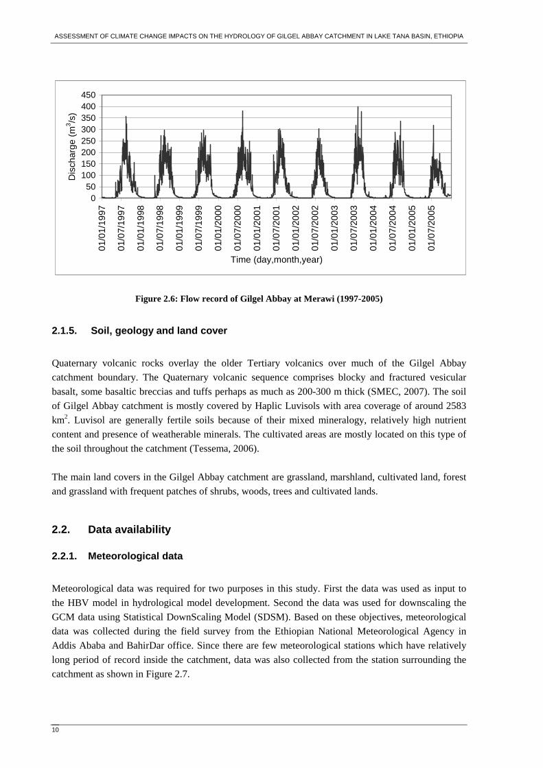
Figure 2.6: Flow record of Gilgel Abbay at Merawi (1997-2005)
2.1.5. Soil, geology and land cover
Quaternary volcanic rocks overlay the older Tertiary volcanics over much of the Gilgel Abbay
catchment boundary. The Quaternary volcanic sequence comprises blocky and fractured vesicular
basalt, some basaltic breccias and tuffs perhaps as much as 200-300 m thick (SMEC, 2007). The soil
of Gilgel Abbay catchment is mostly covered by Haplic Luvisols with area coverage of around 2583
km2. Luvisol are generally fertile soils because of their mixed mineralogy, relatively high nutrient
content and presence of weatherable minerals. The cultivated areas are mostly located on this type of
the soil throughout the catchment (Tessema, 2006).
The main land covers in the Gilgel Abbay catchment are grassland, marshland, cultivated land, forest
and grassland with frequent patches of shrubs, woods, trees and cultivated lands.
2.2. Data availability
2.2.1. Meteorological data
Meteorological data was required for two purposes in this study. First the data was used as input to
the HBV model in hydrological model development. Second the data was used for downscaling the
GCM data using Statistical DownScaling Model (SDSM). Based on these objectives, meteorological
data was collected during the field survey from the Ethiopian National Meteorological Agency in
Addis Ababa and BahirDar office. Since there are few meteorological stations which have relatively
long period of record inside the catchment, data was also collected from the station surrounding the
catchment as shown in Figure 2.7.

ASSESSMENT OF CLIMATE CHANGE IMPACTS ON THE HYDROLOGY OF GILGEL ABBAY CATCHMENT IN LAKE TANA BASIN, ETHIOPIA
11
• Meteorological station
▪ Gauging station
Figure 2.7: Meteorological and gauging station
The number of meteorological variables collected varies from station to station depending on the class
of the stations that are grouped into three. The first group of stations contain only rainfall data. The
second group include maximum and minimum temperature in addition to rainfall data. There are also
stations which contain variables like humidity, sunshine hours, and wind speed in addition to rainfall,
maximum temperature and minimum temperature.
Table 2.1: List of station name, location and meteorological variables
No Station
Name
Latitude
(degree)
Longitude
(degree) Rainfall
Max
Temp
Min
Temp
Relative
humidity
Wind
speed
Sunshine
hours
1 Sekela 11 37.22 √
2 Gundil 10.95 37.07 √ √ √
3 Dangila 11.12 36.83 √ √ √ √ √ √
4
Abay
Shelko 11.38 36.87 √ √ √
5 Kidamaja 11 36.8 √ √ √
6 Zege 11.68 37.32 √ √ √
7 BahirDar 11.6 37.42 √ √ √ √ √ √
8 Adet 11.27 37.47 √ √ √ √ √ √
9 Enjebara 10.97 36.9 √

ASSESSMENT OF CLIMATE CHANGE IMPACTS ON THE HYDROLOGY OF GILGEL ABBAY CATCHMENT IN LAKE TANA BASIN, ETHIOPIA
12
The length of data collected also varies greatly from station to station. There are few stations which
have long continuous records. The only station which has data for more than 25 years in the study
area is BahirDar meteorological station for rainfall, maximum temperature and minimum temperature.
Dangila and Enjebara station have relatively long period of records. All stations listed above contain
daily rainfall data for at least ten years. Therefore all stations were used for hydrological model
development. However, for deriving statistical relationships between the predictand and predictor
long period of records are required. Hence downscaling experiments have been executed based on
BahirDar meteorological data which fulfil all input requirements for SDSM.
2.2.2. Hydrological data
The streamflow of Gilgel Abbay River was required for calibrating and validating the model. There
are two main gauging stations (Gilgel Abbay at Merawi and Koga at Merawi) inside the catchment
which have continuous record for a relatively long period and therefore daily streamflow data (1973-
2005) for these stations were collected during the field work from the Hydrology Department of
Ministry of Water resources.
2.2.3. Remote sensing data
The HBV-96 model can be applied as a semi distributed model, hence the catchment was divided into
different subbasins where the subbasin further divided in elevation and vegetation zones. Based on
this, a digital elevation model of the catchment was prepared using Shuttle Radar Topography
Mission (SRTM) with resolution of 90 m and the DEM was processed using DEM hydroprocessing to
extract drainage area, drainage network and to divide the area into different subbasins and elevation
zones. Moreover, an ASTER image together with ground truth collected during field survey was used
to classify the catchment in different vegetation zones (forest and field) to use as input in the HBV
model.
2.2.4. Climate scenario data
Climate scenario data is required to quantify the relative change of climatic variables between the
current and future time horizon which in turn is used as input to hydrological model for assessment of
hydrological impacts. The climate scenario data used for statistical downscaling model (SDSM) was
obtained from the Canadian Institute for climate studies website for model output of HadCM3
(http://www.cics.uvic.ca/scenarios/sdsm/select.cgi). The predictor variables (see Table 4.1) are
supplied on a grid by grid basis so that the data was downloaded from the nearest grid box to the study
area.

ASSESSMENT OF CLIMATE CHANGE IMPACTS ON THE HYDROLOGY OF GILGEL ABBAY CATCHMENT IN LAKE TANA BASIN, ETHIOPIA
13
3. LITERATURE REVIEW
3.1. Climate model
The Earth’s climate is governed by the interaction between many processes in the atmosphere, ocean,
land surface and cryosphere. The interactions are complex and extensive so that quantitative
predictions of the impact on the climate of greenhouse gas increase cannot be made through simple
intuitive reasoning. For this reason, computer models have been developed which try to
mathematically simulate the climate system, including the interaction between the system component
(Dibike & Coulibaly, 2004). For climate simulation, the major components of the climate system that
must be represented in submodels are atmosphere, ocean, land surface, cryosphere and biosphere,
along with the processes that go on within and between them.
The mathematical models generally used to simulate the present climate and project future climate
with forcing by greenhouse gases and aerosols are generally referred to as GCMs (General Circulation
Models). General Circulation Models in which the atmosphere and ocean components have been
coupled are also known as Atmosphere-Ocean General Circulation Models (AOGCMs). Currently, the
resolution of the atmospheric part of a typical model is about 250 km in the horizontal and about 1 km
in the vertical above the boundary layer. The resolution of a typical ocean model is about 200 to 400
m in the vertical, with a horizontal resolution of about 125 to 250 km. Many physical processes, such
as those related to clouds or ocean convection, take place at much smaller spatial scales than the
model grid and therefore cannot be modelled and resolved explicitly. Their average effects are
approximately included in a simple way by taking advantage of physically based relationships with
the larger-scale variables through the techniques of parameterizations (Houghton, 2001).
Figure 3.1: Schematic view of the processes and interaction in the global climate system (based on Hadley Centre for Climate Prediction and Research)

ASSESSMENT OF CLIMATE CHANGE IMPACTS ON THE HYDROLOGY OF GILGEL ABBAY CATCHMENT IN LAKE TANA BASIN, ETHIOPIA
14
3.1.1. The Climatological baseline
In order to have a basis for assessing future impacts of climate change, it is necessary to obtain a
quantitative description of the changes to be expected. However, before considering future climate it
is important to characterize the present-day or recent climate in a region-often referred to as the
climatological baseline. This baseline period is needed to define the observed climate with which
climate change information is usually combined to create a climatic scenario. When using climate
model results for scenario construction, the baseline serves as the reference period from which the
modelled future change in climate is calculated (Houghton, 2001). The choice of baseline period has
often been governed by availability of the required climate data. The baseline period is usually
selected according to the following criteria (Carter, 2007):
• representative of the present-day or recent average climate in the study region;
• of a sufficient duration to encompass a range of climatic variations, including number of
significant weather anomalies (e.g. severe droughts or cool seasons);
• covering a period for which data on all major climatological variables are abundant,
adequately distributed over space and readily available;
• including data of sufficiently high quality for use in evaluating impacts.
A popular climatological baseline period is the non-overlapping 30-year “normal” period as defined
by the World Meteorological Organization (WMO). The current WMO normal period is 1961-1990.
There are a number of alternative source of baseline climatological data that can be applied in impact
assessments (Carter, 2007). These are not mutually exclusive, and include:
I. National meteorological agencies and archives
II. Supranational and global data sets
III. Climate model outputs
IV. Weather generators
I National meteorological agencies and archives The most common source of observed climatological data applied in impact assessments are the
national meteorological agencies. These agencies usually have the responsibility for the day-to-day
operation and maintenance of the national meteorological observation networks for the purposes of
weather forecasting and other public services.
II Supranational and global data sets As well as serving national needs, climatological data from different countries have also been
combined into various supranational and global data sets. The data sets include observations of
surface variables at a monthly time step over land and ocean, surface and upper air observations at a
daily time step from sites across certain regions and, for recent decades, satellite observations.
III Climate model outputs There are two types of information from global climate models that may be also useful in describing
ASSESSMENT OF CLIMATE CHANGE IMPACTS ON THE HYDROLOGY OF GILGEL ABBAY CATCHMENT IN LAKE TANA BASIN, ETHIOPIA
15
the climatological baselines: reanalysis data and output from GCM and RCM.
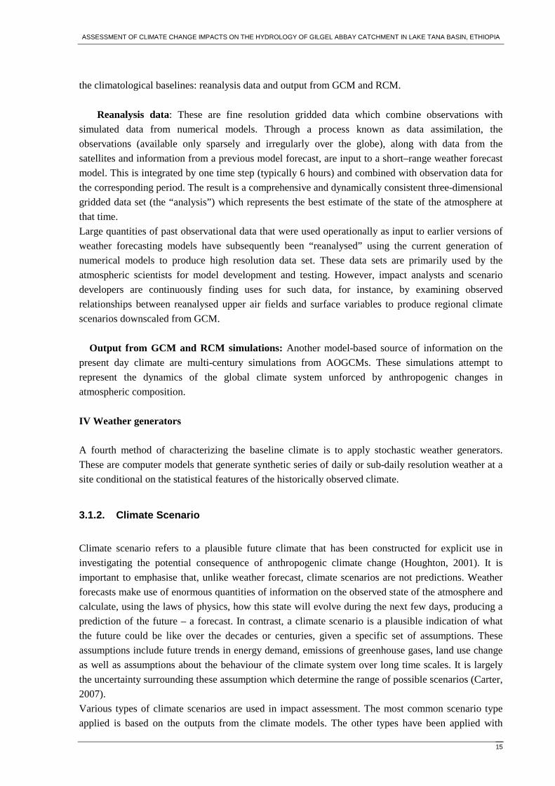
Reanalysis data: These are fine resolution gridded data which combine observations with
simulated data from numerical models. Through a process known as data assimilation, the
observations (available only sparsely and irregularly over the globe), along with data from the
satellites and information from a previous model forecast, are input to a short–range weather forecast
model. This is integrated by one time step (typically 6 hours) and combined with observation data for
the corresponding period. The result is a comprehensive and dynamically consistent three-dimensional
gridded data set (the “analysis”) which represents the best estimate of the state of the atmosphere at
that time.
Large quantities of past observational data that were used operationally as input to earlier versions of
weather forecasting models have subsequently been “reanalysed” using the current generation of
numerical models to produce high resolution data set. These data sets are primarily used by the
atmospheric scientists for model development and testing. However, impact analysts and scenario
developers are continuously finding uses for such data, for instance, by examining observed
relationships between reanalysed upper air fields and surface variables to produce regional climate
scenarios downscaled from GCM.
Output from GCM and RCM simulations: Another model-based source of information on the
present day climate are multi-century simulations from AOGCMs. These simulations attempt to
represent the dynamics of the global climate system unforced by anthropogenic changes in
atmospheric composition.
IV Weather generators A fourth method of characterizing the baseline climate is to apply stochastic weather generators.
These are computer models that generate synthetic series of daily or sub-daily resolution weather at a
site conditional on the statistical features of the historically observed climate.
3.1.2. Climate Scenario
Climate scenario refers to a plausible future climate that has been constructed for explicit use in
investigating the potential consequence of anthropogenic climate change (Houghton, 2001). It is
important to emphasise that, unlike weather forecast, climate scenarios are not predictions. Weather
forecasts make use of enormous quantities of information on the observed state of the atmosphere and
calculate, using the laws of physics, how this state will evolve during the next few days, producing a
prediction of the future – a forecast. In contrast, a climate scenario is a plausible indication of what
the future could be like over the decades or centuries, given a specific set of assumptions. These
assumptions include future trends in energy demand, emissions of greenhouse gases, land use change
as well as assumptions about the behaviour of the climate system over long time scales. It is largely
the uncertainty surrounding these assumption which determine the range of possible scenarios (Carter,
2007).
Various types of climate scenarios are used in impact assessment. The most common scenario type
applied is based on the outputs from the climate models. The other types have been applied with

ASSESSMENT OF CLIMATE CHANGE IMPACTS ON THE HYDROLOGY OF GILGEL ABBAY CATCHMENT IN LAKE TANA BASIN, ETHIOPIA
16
reference to, or in conjunction, with model-based scenarios, namely: incremental scenario for
sensitivity studies and analogue scenarios.
The suitability of each type of scenario for use in policy relevant impact assessment can be assessed
according to five criteria (Houghton, 2001):
1. Consistency at regional level with global projections: Scenario changes in the regional
climate may lie outside the range of global mean changes but should be consistent with
theory and model based results.
2. Physical plausibility and realism: Changes in climate should be physically plausible, such
that changes in different climatic variables are mutually consistent and credible.
3. Appropriateness of information for impact assessments: Scenarios should present climate
changes at an appropriate temporal and spatial scale, for a sufficient number of variables, and
over an adequate time horizon to allow for impact assessment.
4. Representativeness of the potential range of future regional climate change.
5. Accessibility: The information required for developing climate scenarios should be readily
available and easily accessible for use in impact assessment.
I Incremental scenario: Incremental scenarios describe techniques where a particular climate (or
related) elements are changed by arbitrary amounts. For example, adjustments of baseline temperature
by +1, +2, +3, +4ºC and baseline precipitation by± 5, 10, 15 and 20 percent could represent various
magnitude of future change (Carter, 2007).
Incremental scenarios provide information on an ordered range of climate changes and can readily be
applied in a consistent and replicable way in different studies and regions, allowing for direct inter-
comparison of results. However, such scenarios do not necessarily present a realistic set of changes
that are physically plausible. They are usually adopted for exploring system sensitivity prior to the
application of more credible, model based scenario (Houghton, 2001).
II Analogue scenario: Analogue scenarios are constructed by identifying recorded climate regimes
which may resemble the future climate in a given region. Both temporal and spatial analogues have
been used in constructing climate scenarios. Temporal analogues make use of climatic information
from the past as analogue of possible future climate. Spatial analogues are regions which today have a
climate analogues to that anticipated in the study region in the future. Since the causes of the analogue
climate are most likely due to changes in the atmospheric circulation, rather than to greenhouse gas
induced climate change, these types of scenarios are not ordinarily recommended to represent the
future climate in quantitative impact assessments.
III Scenarios based on outputs from climate models: Climate models at different spatial scales and
levels of complexity provide the major source of information for constructing scenarios. The most
common method of developing climate scenarios for quantitative impact assessment is to use results
from General Circulation Models (GCMs). These are numerical models representing physical
processes in the atmosphere, ocean, cryosphere and land surface and considered as the most advanced
tools currently available for simulating the response of the global climate system to increasing
greenhouse gas concentrations. GCMs depict the climate using a three dimensional grid over the

ASSESSMENT OF CLIMATE CHANGE IMPACTS ON THE HYDROLOGY OF GILGEL ABBAY CATCHMENT IN LAKE TANA BASIN, ETHIOPIA
17
globe, typically having a horizontal resolution of between 250 and 600 km, 10 to 20 vertical layers in
the atmosphere and sometimes as many as 30 layers.
The evolving (transient) pattern of climate response to gradual changes in atmospheric composition
was introduced into climate scenarios using the outputs from Coupled Atmosphere-Ocean Models
from the early 1990s onwards. Recent AOGCM simulations begin by modelling historical forcing by
greenhouse gases and aerosols from the 19th or early 20th century onwards. Climate scenarios based on
these simulations are being increasingly adopted in impact studies. However, there are several
limitations that restrict the usefulness of AOGCM outputs for impact assessment (Houghton, 2001):
I. the large resources required to undertake GCM simulations and store their outputs, which
have restricted the range of experiments that can be conducted;
II. their coarse spatial resolution compared to the scale of many impact assessments;
III. the difficulty of distinguishing an anthropogenic signal from the noise of natural internal
model variability;
IV. the difference in climate sensitivity between the models.
The source of the various scenario and their mutual linkages discussed above is shown in Figure 3.2.
Figure 3.2: Some alternative data sources and procedures for constructing climate scenarios for use in impact assessment. Highlighted boxes indicate the baseline climate and common types of scenario. Grey shading encloses the typical component of climate scenario generators (Houghton, 2001)

ASSESSMENT OF CLIMATE CHANGE IMPACTS ON THE HYDROLOGY OF GILGEL ABBAY CATCHMENT IN LAKE TANA BASIN, ETHIOPIA
18
3.1.3. Source of GCM and Emission Scenario
Source of GCM The Intergovernmental Panel on Climate Change (IPCC) Data Distribution Centre (DDC) was
established in 1998 by the World Meteorological Organization and the United Nations Environmental
Programme, following a recommendation by the Task group on Data and Scenario Support for Impact
and Climate Assessment, to facilitate the timely distribution of a consistent set of up-to-date scenarios
of changes in climate and related environmental and socio-economic factor for use in impact and
adaptation assessment.
Therefore the result from the following modelling centre can be found through IPCC DDC.
Table 3.1: Coupled Atmospheric General Circulation Models for which climate change simulations held by the IPCC Data Distribution Centre (Carter, 2007)
Modelling centre country Model(s)
Commonwealth Scientific and Industrial Research
Organization (CSIRO)
Australia CSIRO-Mk2
Max Planck Institut fur Meteorologie (formerly Deutsches
Klimarechenzentrum, DKRZ)
Germany ECHAM4/OPYC and
ECHAM3/LSG
Hadley Centre for Climate Prediction and Research UK HadCM2 and HadCM3
Canadian Centre for Climate modelling and Analysis
(CCCMA)
Canada CGCM1 and CGCM2
Geophysical Fluid Dynamics Laboratory (GFDL) USA GFDL-R15 and GFDL-
R30
National Centre for Atmospheric Research (NCAR) USA NCAR DOE-PCM
Centre for Climate Research Studies (CCSR) and National
Institute for Environmental Studies (NIES)
JAPAN CCSR-NIES
The full sets of monthly results from the experiment (and more detailed technical information) can be
obtained from the DDC GCM Archive (http://www.ipcc-data.org/index.html, 2007). However, daily
fields are only available directly from the respective modelling centres. For example the UK Hadley
Centre archived over 20 daily variables from their HadCM3SRES A2 and B2 experiments (including
temperature, humidity, energy and dynamic variables at several levels in the atmosphere). Some
groups, such as the Canadian Climate Impacts Scenarios (CCIS) project have begun supplying gridded
predictor variables on-line (http://www.cics.uvic.ca/scenarios/sdsm/select.cgi) for the specific needs
of the downscaling community. In addition, a large suite of secondary variables such as atmospheric
stability, vorticity, divergence, zonal and meridional airflows may be derived from standard daily
variables such as mean sea level pressure or geopotential height (Wilby et al., 2004).
Emission scenario In 1996, the IPCC began the development of a new set of emission scenarios, effectively to update
and replace the well-known IS92 scenarios. The approved new set of scenarios is described in the
ASSESSMENT OF CLIMATE CHANGE IMPACTS ON THE HYDROLOGY OF GILGEL ABBAY CATCHMENT IN LAKE TANA BASIN, ETHIOPIA
19
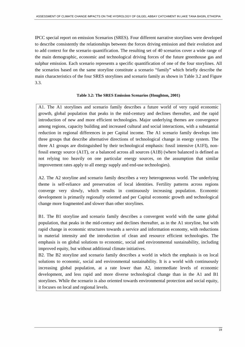
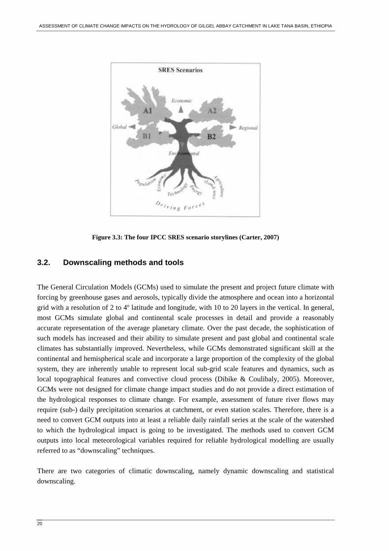
IPCC special report on emission Scenarios (SRES). Four different narrative storylines were developed
to describe consistently the relationships between the forces driving emission and their evolution and
to add context for the scenario quantification. The resulting set of 40 scenarios cover a wide range of
the main demographic, economic and technological driving forces of the future greenhouse gas and
sulphur emission. Each scenario represents a specific quantification of one of the four storylines. All
the scenarios based on the same storyline constitute a scenario “family” which briefly describe the
main characteristics of the four SRES storylines and scenario family as shown in Table 3.2 and Figure
3.3.
Table 3.2: The SRES Emission Scenarios (Houghton, 2001)
A1. The A1 storylines and scenario family describes a future world of very rapid economic
growth, global population that peaks in the mid-century and declines thereafter, and the rapid
introduction of new and more efficient technologies. Major underlying themes are convergence
among regions, capacity building and increased cultural and social interactions, with a substantial
reduction in regional differences in per Capital income. The A1 scenario family develops into
three groups that describe alternative directions of technological change in energy system. The
three A1 groups are distinguished by their technological emphasis: fossil intensive (A1FI), non-
fossil energy source (A1T), or a balanced across all sources (A1B) (where balanced is defined as
not relying too heavily on one particular energy sources, on the assumption that similar
improvement rates apply to all energy supply and end-use technologies).
A2. The A2 storyline and scenario family describes a very heterogeneous world. The underlying
theme is self-reliance and preservation of local identities. Fertility patterns across regions
converge very slowly, which results in continuously increasing population. Economic
development is primarily regionally oriented and per Capital economic growth and technological
change more fragmented and slower than other storylines.
B1. The B1 storyline and scenario family describes a convergent world with the same global
population, that peaks in the mid-century and declines thereafter, as in the A1 storyline, but with
rapid change in economic structures towards a service and information economy, with reductions
in material intensity and the introduction of clean and resource efficient technologies. The
emphasis is on global solutions to economic, social and environmental sustainability, including
improved equity, but without additional climate initiatives.
B2. The B2 storyline and scenario family describes a world in which the emphasis is on local
solutions to economic, social and environmental sustainability. It is a world with continuously
increasing global population, at a rate lower than A2, intermediate levels of economic
development, and less rapid and more diverse technological change than in the A1 and B1
storylines. While the scenario is also oriented towards environmental protection and social equity,
it focuses on local and regional levels.
ASSESSMENT OF CLIMATE CHANGE IMPACTS ON THE HYDROLOGY OF GILGEL ABBAY CATCHMENT IN LAKE TANA BASIN, ETHIOPIA
20
Figure 3.3: The four IPCC SRES scenario storylines (Carter, 2007)
3.2. Downscaling methods and tools
The General Circulation Models (GCMs) used to simulate the present and project future climate with
forcing by greenhouse gases and aerosols, typically divide the atmosphere and ocean into a horizontal
grid with a resolution of 2 to 4º latitude and longitude, with 10 to 20 layers in the vertical. In general,
most GCMs simulate global and continental scale processes in detail and provide a reasonably
accurate representation of the average planetary climate. Over the past decade, the sophistication of
such models has increased and their ability to simulate present and past global and continental scale
climates has substantially improved. Nevertheless, while GCMs demonstrated significant skill at the
continental and hemispherical scale and incorporate a large proportion of the complexity of the global
system, they are inherently unable to represent local sub-grid scale features and dynamics, such as
local topographical features and convective cloud process (Dibike & Coulibaly, 2005). Moreover,
GCMs were not designed for climate change impact studies and do not provide a direct estimation of
the hydrological responses to climate change. For example, assessment of future river flows may
require (sub-) daily precipitation scenarios at catchment, or even station scales. Therefore, there is a
need to convert GCM outputs into at least a reliable daily rainfall series at the scale of the watershed
to which the hydrological impact is going to be investigated. The methods used to convert GCM
outputs into local meteorological variables required for reliable hydrological modelling are usually
referred to as “downscaling” techniques.
There are two categories of climatic downscaling, namely dynamic downscaling and statistical
downscaling.
ASSESSMENT OF CLIMATE CHANGE IMPACTS ON THE HYDROLOGY OF GILGEL ABBAY CATCHMENT IN LAKE TANA BASIN, ETHIOPIA
21
3.2.1. Dynamic downscaling
Dynamic downscaling is a method of extracting local-scale information by developing and using
limited-area models (LAMs) or regional climate models (RCMs) with the coarse GCM data used as
boundary condition. The basic steps are then to use the GCMs to simulate the response of the global
circulation to large-scale forcing and RCM to account for sub-GCM grid scale forcing such as
complex topographical features and land cover heterogeneity in a physically-based way, and thus
enhance the simulation of atmospheric circulations and climate variables at fine spatial scales. RCMs
have recently been developed that can attain horizontal resolution in the order of tens of kilometres or
less over selected areas of interest. Despite the fact that the resolution of RCM is finer than the GCM,
there are several acknowledged limitations. RCMs still require considerable computing resources and
are as expensive to run as a global GCM. Moreover these models cannot meet the needs of spatially
explicit models of hydrological systems. Hence there remains the need to downscale the results from
such models to individual sites or localities for impact studies (Xu, 1999).
3.2.2. Empirical (statistical) downscaling
Empirical (statistical) downscaling involves developing a quantitative relationship between large-
scale atmospheric variables (predictors) and local surface variables (predictands). From this
perspective, regional or local climate information is derived by first determining a statistical model
which relates large-scale climate variables (or “predictor”) to regional and local variables (or
“predictands”). Then the large-scale output of a GCM simulation is fed into the statistical model to
estimate the corresponding local and regional climate characteristics.
The most common form has the predictand as a function of the predictor(s). The concept of regional
climate being conditioned by the large-scale state may be written as:
R = F(L) (1)
Where, R represents the predictand (a regional or local climate variables), L is the predictor (a set of
large-scale climate variables), and F is a deterministic/stochastic function conditioned by L and has to
be found empirically from observation or modelled data sets.
Most statistical downscaling work has focussed on single-site (i.e. point scale) daily precipitation as
the predictand because it is the most important input variable for many natural systems models and
cannot be obtained directly from climate model output. Predictor sets are typically derived from sea
level pressure, geopotential height, wind fields, absolute or relative humidity, and temperature
variables (Wilby et al., 2004).
One of the primary advantages of the statistical downscaling method is that they are computationally
inexpensive and thus can be easily applied to output from different GCM experiments. Another
advantage is that they can be used to provide site-specific information, which can be critical for many
climate change studies. The major theoretical weakness of statistical downscaling is that their basic
assumption is not verifiable, i.e. the statistical relationships developed for the present day climate also
hold under the different forcing conditions of possible future climates (Wilby et al., 2004). Despite
this limitation, statistical downscaling is applied in this study because this method require less

ASSESSMENT OF CLIMATE CHANGE IMPACTS ON THE HYDROLOGY OF GILGEL ABBAY CATCHMENT IN LAKE TANA BASIN, ETHIOPIA
22
computational resource and less knowledge of atmospheric chemistry compared to dynamic
downscaling method.
A diverse range of empirical/statistical downscaling techniques have been developed over the past
few years and each method lies in one of the three major categories, namely, regression (transfer
function) methods, stochastic weather generators and weather typing schemes.
I Regression model
Regression-based downscaling methods rely on direct quantitative relationship between the local scale
climate variables (predictand) and the variables containing the large scale climate information
(predictors) through some form of regression functions. Individual downscaling schemes differ
according to the choice of mathematical transfer function, predictor variables or statistical fitting
procedure.
One of the well recognized statistical downscaling tools that implements a regression based method is
the Statistical Down-Scaling Models (SDSM). SDSM 4.1 facilitates the rapid development of
multiple, low cost, single-site scenarios of daily surface weather variables under the present and future
climate forcing. Additionally, the software performs ancillary tasks of data quality control and
transformation, predictor variables pre-screening, automatic model calibration, basic diagnostic
testing, statistical analyses and graphing of climate data (Dawson & Wilby, 2007).
II Stochastic weather generators
Weather generators (WGs) are models that replicate the statistical attribute of local climate variables
(such as the mean and variance) but not observed sequence of events. These models are based on the
representations of precipitation occurrence via Markov processes for wet-/dry or spell transitions.
Secondary variables such as wet-day amounts, temperatures and solar radiation are often modelled
conditional on precipitation occurrence. WGs are adapted for statistical downscaling by conditioning
their parameters on large-scale atmospheric predictors, weather states or rainfall properties (Wilby et
al., 2004).
One well known stochastic downscaling tool for use in climate impact studies is the Long Ashton
Research Station Weather Generator (LARS-WG). LARS-WG is a stochastic weather generator
which can be used for the simulation of weather data at a single site under both current and future
climate condition. These data are in the form of daily time-series for a suite of climate variables,
namely precipitation (mm), maximum and minimum temperature (ºC) and solar radiation(MJm-2day-1)
(Semenov, 2002).
III Weather typing scheme
Weather classification methods group days into a finite number of discrete weather types or “states”
according to their synoptic similarity. Typically, weather states are defined by applying cluster
analysis to atmospheric fields or using subjective circulation classification schemes (Wilby et al.,
2004).

ASSESSMENT OF CLIMATE CHANGE IMPACTS ON THE HYDROLOGY OF GILGEL ABBAY CATCHMENT IN LAKE TANA BASIN, ETHIOPIA
23
3.3. Hydrological model
3.3.1. Use of hydrological modelling in climate change impact studies
Hydrological models are mathematical formulations which determine the runoff signal which leaves a
watershed basin from the rainfall signal received by this basin. They provide a means of quantitative
prediction of catchment runoff that may be required for efficient management of water resources.
Such hydrological models are also used as means of extrapolating from those available measurements
in both space and time into the future to assess the likely impact of future hydrological change.
Changes in global climate are believed to have significant impacts on local hydrological regimes, such
as in streamflows which support aquatic ecosystem, navigation, hydropower, irrigation system, etc. In
addition to the possible changes in total volume of flow, there may also be significant changes in
frequency and severity of floods and droughts. Hence hydrological models provide a framework to
conceptualize and investigate the relationship between climate and water resource.
Chong-vu Xu mention the advantages of hydrological models in climate change impact studies as
follows (Xu, 1999):
1. Models tested for different climatic/physiographic conditions, as well as models structured
for use at various spatial scales and dominant process representations, are readily available.
2. GCM-derived climate perturbations (at different level of downscaling) can be used as model
input.
3. A variety of response to climate change scenarios can be modelled.
4. The models can convert climate change output to relevant water resource variables related,
for example, to reservoir operation, irrigation demand, drinking and water supply.
An investigation of climate-change effects on regional water resources consists of the following three
steps: (1) using climate models to simulate climatic effect of increased atmospheric concentration of
greenhouse gases, (2) using downscaling techniques to link climate models and catchment-scale
hydrological models or to provide catchment-scale climate scenarios as input to hydrological models,
and (3) using hydrological models to simulate hydrological impacts of climate change.
Many investigations were done in the past two decades on the application of hydrological model for
assessment of the potential effect of climate change on variety of water resource issues. These
investigations can range from the evaluation of annual and seasonal streamflow variation using simple
water-balance models to the evaluation of variations in surface and groundwater quantity, quality and
timing using complex distributed-parameter model that simulate a wide range of water, energy and
biochemical processes. Based on the level of complexity, these models can be grouped into four
categories: (1) Empirical models (annual base), (2) Water-balance models (monthly), (3) Conceptual
lumped-parameter models (daily), and (4) Process-based distributed models (hourly or finer base).
The choices of a model for a particular case study depend on many factors, the purpose of the study
and model availability being the dominant ones. For detailed assessment of surface flow, conceptual
models were applied in many parts of the world. Booij,(2005) discusses the advantages of conceptual

ASSESSMENT OF CLIMATE CHANGE IMPACTS ON THE HYDROLOGY OF GILGEL ABBAY CATCHMENT IN LAKE TANA BASIN, ETHIOPIA
24
models for climate change study as a nice compromise between the need for simplicity on one hand
and the need for a firm physical basis on the other hand. One of the more frequently used conceptual
model for climate change impact study is the HBV model. The HBV model is widely used in Nordic
countries as a tool to assess the climate change effects. Climate change impact on runoff and
hydropower in the Nordic countries have been studied by using the HBV models (Xu, 1999).
Booij,(2005) applied the HBV model to assess the impact of climate change on river flooding on
Meuse River in the Netherlands. Dibike and Coulibaly,(2005) applied the HBV model to study the
hydrological impact of climate change in the Saguenay watershed in Canada.
In conclusion, the HBV model is selected for this study because of the following reason:
1. the input data requirement is moderate;
2. the model simulate the major hydrological process in the catchments;
3. the model was tested for the impact of climate change on hydrological study in different
parts of the world and
4. the availability of the model
3.3.2. Short description of the HBV model
The HBV model is a conceptual hydrological model for continuous calculation of runoff. It was
originally developed at the Swedish Meteorological and Hydrological Institute (SMHI) in the early
1970s. Since then the model has found application in more than 40 countries. Originally the HBV
model was developed for runoff simulation and hydrological forecasting, but the scope of the
application has increased steadily. Today the HBV model can be used (Seibert, 2002):
• for water balance studies;
• for runoff forecasting (flood warning and reservoir operation);
• to compute design floods for dam safety;
• to investigate the effects of changes with in the catchmnent;
• to simulate climate change effects.
In 1993 the Swedish Association of River Regulation Enterprises (VASO) and SMHI initiated a major
revision of the structure of the HBV model with the same philosophy of simplicity as the original
HBV model to make the model more physically reasonable and up-to-date with the current
hydrological and meteorological knowledge. HBV-96 is the final result of this model revision.
The HBV-96 is best described as a semi-distributed conceptual model. The model simulates daily
discharge using daily rainfall, temperature and estimates of potential evapotranspiration as input
together with geographic information about the river catchment. The evapotranspiration values used
are long-term monthly averages. Discharge observations are used to calibrate the model, and to verify
and correct the model before a runoff forecast. The model consists of subroutines for snow
accumulation and melt, soil moisture accounting procedure, routines for runoff generation and finally,
a simple routing procedure.
It is possible to run the model separately for several subbasins and then add the contributions from all
subbasins. Calibration as well as forecasts can be made for each subbasin. For basin of considerable

ASSESSMENT OF CLIMATE CHANGE IMPACTS ON THE HYDROLOGY OF GILGEL ABBAY CATCHMENT IN LAKE TANA BASIN, ETHIOPIA
25
elevation range a subdivision into elevation zones can be made. Each elevation zone can further be
divided into different vegetation zones (forested and non-forested areas). A schematic sketch of the
HBV-96 model is shown in Figure 3.4.
Figure 3.4: Schematic structure of HBV-96 model
Precipitation and snowmelt Precipitation calculations are made separately for each elevation/ vegetation
zone within a subbasin.
To separate between snow and rainfall a threshold temperature is used:
RF = Pcorr·rfcf·P if T>tt (2)
SF = Pcorr·sfcf·P if T<tt (3)

ASSESSMENT OF CLIMATE CHANGE IMPACTS ON THE HYDROLOGY OF GILGEL ABBAY CATCHMENT IN LAKE TANA BASIN, ETHIOPIA
26
Where,
RF = rainfall
SF = snowfall
P = observed precipitation (mm)
T = observed temperature (ºC)
tt = threshold temperature (ºC)
Rfcf = rainfall correction factor
Sfcf = snowfall correction factor
Pcorr = general precipitation correction factor
Soil routine The soil moisture accounting routine is the main part controlling runoff formation. This routine is
based on three parameters,β , LP and FC as shown in Figure 3.4. β control the contribution to the
response function (∆Q/∆P) or the increase in soil moisture storage (1-∆Q/∆P) from each millimetre of
rainfall or snow melt. The ratio ∆Q/∆P is often called runoff coefficient, and ∆Q is often called
effective precipitation. ∆Q/∆P can also be expressed as R/IN. LP is the soil moisture value above
which evapotranspiration reaches its potential value, and FC is the maximum soil moisture storage (in
mm) in the model.
The effect of the soil routine is that the contribution to runoff from rain or snow melt is small when
the soil is dry (low soil moisture values), and great at wet conditions. The actual evapotranspiration
decreases as the soil dries out. Long-term mean values are used as estimates of the potential
evapotranspiration at a certain time of the year.
Response routine The runoff generation routine is the response functions which transform excess water from the soil
moisture zone to runoff. It also includes the effect of direct precipitation and evapotranspiration on a
part which represents lakes, rivers and other wet areas. The function consists of one upper, non-linear,
and one lower, linear, reservoir. These are the origin of the quick and slow runoff components of the
hydrograph.
The yield from the soil moisture zone, i.e. the effective precipitation, will be added to the storage in
the upper reservoir. As long as there is water in the upper reservoir, water will percolate to the lower
reservoir according to the parameter PERC. At high yield from the soil, percolation is not sufficient to
keep the upper reservoir empty, and the generated discharge will have a contribution directly from the
upper reservoir which represents drainage through more superficial channels. The lower reservoir, on
the other hand, represents the groundwater storage of the catchment contributing to the baseflow.

ASSESSMENT OF CLIMATE CHANGE IMPACTS ON THE HYDROLOGY OF GILGEL ABBAY CATCHMENT IN LAKE TANA BASIN, ETHIOPIA
27
Transformation function The runoff generated from the response routine is routed through a transformation function in order to
get a proper shape of the hydrograph at the outlet of the subbasin. The transformation function is a
simple filter technique with a triangular distribution of the weights.
Calibration and Evaluation of the model result Input data for the calculation are daily values of precipitation and air temperature and potential
evapotranspiration for a representative station of the basin. For the potential evapotranspiration,
normally monthly mean estimates are used, either measured or calculated. During the calibration
period observed discharge values are required for each time step.

ASSESSMENT OF CLIMATE CHANGE IMPACTS ON THE HYDROLOGY OF GILGEL ABBAY CATCHMENT IN LAKE TANA BASIN, ETHIOPIA
28
ASSESSMENT OF CLIMATE CHANGE IMPACTS ON THE HYDROLOGY OF GILGEL ABBAY CATCHMENT IN LAKE TANA BASIN, ETHIOPIA
29
4. METHODOLOGY
An investigation of climate change effect on the hydrological regimes consists of the following three
steps:
1. the development and use of General Circulation Models (GCMs) to provide future global
climate scenarios under the effect of increasing greenhouse gases,
2. the development and use of downscaling techniques for downscaling the GCMs output to
the scales compatible with hydrological models, and
3. the development and use of hydrological models to simulate the effects of climate change
on hydrological regimes at various scale (Xu et al., 2005).
4.1. General Circulation Model (GCM)
The climate model is a mathematical description of the Earth’s climate system, broken into a number
of grid boxes and levels in the atmosphere, ocean and land. At each of these grid points equations are
solved which describe the large-scale balances of the momentum, heat and moisture. Based on this, a
wide range of climate models are developed as listed in Table 3.1. The modelling approach and the
resolution of the model vary from model to model.
The relative performance of GCMs can depend on the size of the region (i.e. small regions at sub-grid
scale are less likely to be well described than large regions at continental scale), on its location (i.e.
the level of agreement between GCM outputs varies a lot from region to region) and on the variables
being analyzed (for instance, regional precipitation is more variable and more difficult to model than
regional temperature) (Carter, 2007).
Even though it is often recommended to use different GCMs and emission scenarios in order to make
comparison between different models, this study does not include such comparison due to limited
amount of time available to complete the study. For this study the model output of HadCM3 was
employed for the A2 (Medium-High Emissions) and B2 (Medium-Low Emission) Scenarios.
HadCM3 is a coupled atmospheric-ocean GCM developed at Hadley Centre for Climate Prediction
and Research, UK. The atmospheric part of HadCM3 has a horizontal resolution of 2.5º latitude x
3.75º longitude, and has 19 vertical levels. The ocean component of the model has 20 vertical levels
with horizontal resolution of 1.25º latitude x1.25º longitude.
HadCM3 is applied in this study because the model is widely applied in many climate change impact
studies and the model provides daily predictor variables which can be used for the Statistical
DownScaling Model.

ASSESSMENT OF CLIMATE CHANGE IMPACTS ON THE HYDROLOGY OF GILGEL ABBAY CATCHMENT IN LAKE TANA BASIN, ETHIOPIA
30
4.2. Statistical DownScaling Model
4.2.1. General description of the model
General Circulation Models indicate that rising concentration of greenhouse gases will have
significant implications for climate at global and regional scales. However, GCMs are restricted in
their use for local impact studies due to the coarse resolution and inability to resolve important sub-
grid scale features such as clouds and topography. As a consequence downscaling techniques have
emerged as a mean of deriving local-scale weather from regional-scale atmospheric predictor
variables (Dawson & Wilby, 2007).
There are various downscaling techniques available to convert GCM outputs into daily meteorological
variables that can be used in hydrological impact studies. However, it is not yet clear which methods
provides the most reliable estimates for the future climate (Dibike & Coulibaly, 2004), since such
methods also depends on the purpose of study, the area of study and data availability. The statistical
downscaling has a number of advantages over the use of raw GCM output. Firstly, the stochasticity of
the model facilitates the generation of ensembles of future climatic realisations that is a pre-requisite
to confidence estimations. Secondly, the downscaling model may be tuned to reproduce the unique
meteorological characteristics of individual stations that is a valuable asset in heterogeneous
landscapes or mountainous terrain. Thirdly, such techniques are far less data intensive and
computationally demanding than dynamic methods (Leavesley et al., 1999). In situations where low-
cost, rapid assessments of localized climate change impacts are required, statistical downscaling
(currently) represents the more promising option (Dawson & Wilby, 2007) despite their limitation in
assumption that the statistical relationships developed for the present climate also hold under the
different forcing condition of the possible future climate.
Figure 4.1: A schematic illustrating the general approach to downscaling (Dawson & Wilby, 2007)
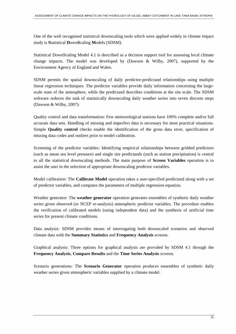
ASSESSMENT OF CLIMATE CHANGE IMPACTS ON THE HYDROLOGY OF GILGEL ABBAY CATCHMENT IN LAKE TANA BASIN, ETHIOPIA
31
One of the well recognized statistical downscaling tools which were applied widely in climate impact
study is Statistical DownScaling Models (SDSM).
Statistical DownScaling Model 4.1 is described as a decision support tool for assessing local climate
change impacts. The model was developed by (Dawson & Wilby, 2007), supported by the
Environment Agency of England and Wales.
SDSM permits the spatial downscaling of daily predictor-predictand relationships using multiple
linear regression techniques. The predictor variables provide daily information concerning the large-
scale state of the atmosphere, while the predictand describes conditions at the site scale. The SDSM
software reduces the task of statistically downscaling daily weather series into seven discrete steps
(Dawson & Wilby, 2007):
Quality control and data transformation: Few meteorological stations have 100% complete and/or full
accurate data sets. Handling of missing and imperfect data is necessary for most practical situations.
Simple Quality control checks enable the identification of the gross data error, specification of
missing data codes and outliers prior to model calibration.
Screening of the predictor variables: Identifying empirical relationships between gridded predictors
(such as mean sea level pressure) and single site predictands (such as station precipitation) is central
to all the statistical downscaling methods. The main purpose of Screen Variables operation is to
assist the user in the selection of appropriate downscaling predictor variables.
Model calibration: The Calibrate Model operation takes a user-specified predictand along with a set
of predictor variables, and computes the parameters of multiple regression equation.
Weather generator: The weather generator operation generates ensembles of synthetic daily weather
series given observed (or NCEP re-analysis) atmospheric predictor variables. The procedure enables
the verification of calibrated models (using independent data) and the synthesis of artificial time
series for present climate conditions.
Data analysis: SDSM provides means of interrogating both downscaled scenarios and observed
climate data with the Summary Statistics and Frequency Analysis screens.
Graphical analysis: Three options for graphical analysis are provided by SDSM 4.1 through the
Frequency Analysis, Compare Results and the Time Series Analysis screens.
Scenario generations: The Scenario Generator operation produces ensembles of synthetic daily
weather series given atmospheric variables supplied by a climate model.

ASSESSMENT OF CLIMATE CHANGE IMPACTS ON THE HYDROLOGY OF GILGEL ABBAY CATCHMENT IN LAKE TANA BASIN, ETHIOPIA
32
NB Bold box indicate the key function of SDSM Figure 4.2: SDSM Version 4.1 climate scenario generation (Dawson & Wilby, 2007)
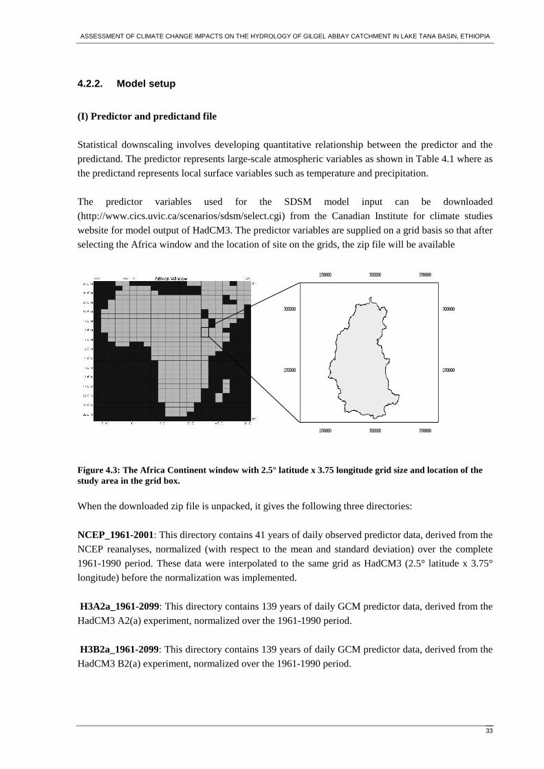
ASSESSMENT OF CLIMATE CHANGE IMPACTS ON THE HYDROLOGY OF GILGEL ABBAY CATCHMENT IN LAKE TANA BASIN, ETHIOPIA
33
4.2.2. Model setup
(I) Predictor and predictand file Statistical downscaling involves developing quantitative relationship between the predictor and the
predictand. The predictor represents large-scale atmospheric variables as shown in Table 4.1 where as
the predictand represents local surface variables such as temperature and precipitation.
The predictor variables used for the SDSM model input can be downloaded
(http://www.cics.uvic.ca/scenarios/sdsm/select.cgi) from the Canadian Institute for climate studies
website for model output of HadCM3. The predictor variables are supplied on a grid basis so that after
selecting the Africa window and the location of site on the grids, the zip file will be available
Figure 4.3: The Africa Continent window with 2.5° latitude x 3.75 longitude grid size and location of the study area in the grid box.
When the downloaded zip file is unpacked, it gives the following three directories:
NCEP_1961-2001: This directory contains 41 years of daily observed predictor data, derived from the
NCEP reanalyses, normalized (with respect to the mean and standard deviation) over the complete
1961-1990 period. These data were interpolated to the same grid as HadCM3 (2.5° latitude x 3.75°
longitude) before the normalization was implemented.
H3A2a_1961-2099: This directory contains 139 years of daily GCM predictor data, derived from the
HadCM3 A2(a) experiment, normalized over the 1961-1990 period.
H3B2a_1961-2099: This directory contains 139 years of daily GCM predictor data, derived from the
HadCM3 B2(a) experiment, normalized over the 1961-1990 period.

ASSESSMENT OF CLIMATE CHANGE IMPACTS ON THE HYDROLOGY OF GILGEL ABBAY CATCHMENT IN LAKE TANA BASIN, ETHIOPIA
34
NCEP data are re-analysis sets from the National Centre for Environmental Prediction which was re-
gridded to match with the grid system of the HadCM3. These are the data used for model calibration.
Both the NCEP and HadCM3 data have daily predictors. The predictor variables which are available
for both NCEP and HadCM3 are shown in Table 4.1.
Table 4.1: Types of predictor variables
The predictand (maximum temperature, minimum temperature and precipitation) for a specific site
can be prepared in the same format as predictor with single column text file to use as input for the
downscaling model.
(II) Setting of the model parameter Year length: The normal calendar year (366) which allows 29 days in February every fourth year is
used whenever dealing with predictand and NCEP predictor whereas the year length of 360 days is
used in the scenario generation part since HadCM3 uses model years consisting of 360 days.
Event Threshold: The event threshold is set to zero for temperature and 0.1 mm/day for precipitation
to treat trace rain days as dry days.
Model Transformation: The model transformation is applied to the predictand in conditional
models. The default (None) is used for the predictand that is normally distributed as in the case of
daily temperature and fourth root transformation is applied for precipitation since the model is
conditional and the data is skewed.
Variance inflation: Variance inflation controls the magnitude of variance inflation in the downscaled
daily weather variables. This parameter can be adjusted during the calibration period to force the
model replicate the observed data. The default value (i.e.12) produces approximately normal variance
No Predictor
variable
Predictor description No Predictor
variable
Predictor description
1 mslpaf mean sea level pressure 14 p5zhaf 500 hpa divergence
2 p_faf surface air flow strength 15 p8_faf 850 hpa airflow strength
3 p_uaf surface zonal velocity 16 p8_uaf 850 hpa zonal velocity
4 p_vaf surface meridional velocity 17 p8_vaf 850 hpa meridional velocity
5 p_zaf surface vorticity 18 p8_zaf 850 hpa vorticity
6 p_thaf surface wind direction 19 p850af 850 hpa geopotential height
7 p_zhaf Surface divergence 20 p8thaf 850 hpa wind direction
8 p5_faf 500 hpa airflow strength 21 p8zhaf 850 hpa divergence
9 p5_uaf 500 hpa zonal velocity 22 p500af Relative humidity at 500 hpa
10 p5_vaf 500 hpa meridional velocity 23 p850af Relative humidity at 850 hpa
11 p5_zaf 500 hpa vorticity 24 rhumaf Near surface relative humidity
12 p500af 500 hpa geopotential height 25 shumaf Surface specific humidity
13 p5thaf 500 hpa wind direction 26 tempaf Mean temperature at 2 m

ASSESSMENT OF CLIMATE CHANGE IMPACTS ON THE HYDROLOGY OF GILGEL ABBAY CATCHMENT IN LAKE TANA BASIN, ETHIOPIA
35
inflation prior to any transformation and is applied to maximum and minimum temperature. For
precipitation this parameter can be adjusted during the calibration period and is set to 18.
Bias correction: Bias correction compensates for any tendency to over or under estimates the mean
of the conditional process by the downscaling model. This parameter is set to1 (default value) for
maximum and minimum temperature since the process is non conditional whereas for precipitation
this parameter can be adjusted in order to match the mean of the conditional process and is set to 0.91.
(III) Screening the downscaling predictor variables The choice of predictor variables is one of the most influential steps in the development of statistical
downscaling procedure. Identifying empirical relationships between gridded predictors and single site
predictands is central to all statistical downscaling. The screen variable option in SDSM assists the
choice of appropriate downscaling predictor variables through seasonal correlation analysis, partial
correlation analysis, and scatterplots. One of the approaches is to choose all predictors and run the
explained variance on a group of eight or ten at a time. Out of the groups, those predictors which have
high explained variance are selected. Then partial correlation analysis is done for selected predictors
to see the level of correlation with each other. There could be a predictor with a high explained
variance but it might be very highly correlated with another predictor. This means that it is difficult to
tell that this predictor will add information to the process and therefore it will be dropped from the
list. Finally the scatterplot indicates whether this result is due to a few outliers or it is a potentially
useful downscaling relationship. For example in selecting the potential predictor for maximum
temperature, there are five predictors which have high explained variance among the twenty-six
predictors. These are ncep temp, ncepp500, ncepr850, ncepp_zh and ncepp5_u. But when these five
predictors are correlated each other through partial correlation analysis, ncepp5_u shows strong
association with another predictor and is therefore dropped from the selection.
Table 4.2: Correlation matrix
Finally the scatterplot reveals that ncepr850 does not indicate a good relationship from the predictand
(maximum temperature) and is therefore dropped from the list. Therefore the potential predictor
variables for downscaling the maximum temperature become nceptemp, ncepp500 and ncep_zh.
Similar analysis was done for the other predictands and the result is shown in Table 4.3.
predictor Partial r P value
ncemtemp 0.494 0.0
ncepp500 0.134 0.0
ncepr850 0.087 0.0
ncep_zh -0.34 0.0
ncepp5_u -0.001 0.5609

ASSESSMENT OF CLIMATE CHANGE IMPACTS ON THE HYDROLOGY OF GILGEL ABBAY CATCHMENT IN LAKE TANA BASIN, ETHIOPIA
36
Table 4.3: Large scale predictor variables selected for SDSM
(IV) Model calibration The calibration model process constructs downscaling models based on multiple regression equations,
given daily weather data (the predictand) and regional-scale, atmospheric (predictor) variables. The
model structure for calibration can be specified by selecting the process either unconditional or
conditional. In unconditional models a direct link is assumed between the predictors and predictand.
In unconditional models, there is an intermediate process between the regional forcing and local
weather (e.g., local precipitation amounts depend on wet-/-dry-day occurrence, which in turn depend
on regional-scale predictors such as humidity and atmospheric pressure). The model structure is set to
unconditional for maximum and minimum temperature and conditional for precipitation. The model
type determines whether individual downscaling models will be calibrated for each calendar months,
climatological season or entire year. The model is structured as a monthly model for both
precipitation and temperature downscaling, in which case, twelve regression equations are derived for
twelve months using different regression parameters for each month equation. Finally the data period
should be set in order to specify the start and end date of the analysis. The calibration was done for a
30 year of period (1961-1990).
(v) Scenario Generator The Scenario Generation operation produces ensembles of synthetic daily weather series given the
regression weight produced during the calibration process and the daily atmospheric predictor
supplied by a GCM (either under the present or future greenhouse gas forcing). Twenty ensembles of
synthetic daily time series were produced for the two emission scenarios (HadCM3A2a and
HadCM3B2a) for a period of 139 years (1961 to 2099). Finally the mean of twenty ensembles for the
specified period is produced for the maximum and minimum temperature and precipitation.
Precipitation downscaling is necessarily more complex than temperature because daily precipitation
amounts at individual sites are relatively poorly resolved by the regional-scale predictors, and
precipitation is a conditional process (i.e. both the occurrence and amount processes must be
specified) (Dawson & Wilby, 2007).
Predictand Predictor sympol
Minimum temperature Mean temperature at 2m
500hpa geopotential height
nceptemp
ncepp500
Maximum
temperature
Mean temperature at 2m
500hpa geopotential height
Surface divergence
nceptemp
ncepp500
ncepp_zh
Precipitation Relative humidity at 500 hpa
Surface meridional velocity
Surface divergence
ncepr500
ncepp_v
ncepp_zh

ASSESSMENT OF CLIMATE CHANGE IMPACTS ON THE HYDROLOGY OF GILGEL ABBAY CATCHMENT IN LAKE TANA BASIN, ETHIOPIA
37
4.3. HBV-96
4.3.1. General description
HBV-96 is a mathematical model of the hydrological processes in a catchment used to simulate the
runoff properties. It can be described as a semi-distributed conceptual model that allows dividing the
catchment into subbasins and the subbasins further divide into elevation and vegetation zones.
The basic philosophy of the model acknowledges that the model complexity and data demand must
not be in conflict with in the operational requirements and can be formulated as follows (Lindstrom et
al., 1997):
• The model shall be based on a sound scientific foundation;
• Data demands must be met in typical basins;
• The model complexity must be justified by model performance;
• The model must be properly validated;
• The model must be understandable by users.
The general water balance of the model is described as:
P-E-Q=dt
d [SP+SM+UZ+LZ+lakes] (4)
Where,
P = precipitation
E = evapotranspiration
Q = runoff
SP = snow pack
SM = soil moisture
UZ = upper groundwater zone
LZ = lower groundwater zone
Lakes = lake volume
The model consists of subroutines for snow accumulation and melt, a soil accounting procedure,
routines for runoff generation and a simple routing procedure. It is possible to run the model
separately for several subbasins and then add the contributions from the entire subbasin. Calibration
as well as forecast can be made for each subbasin. For the basins of considerable elevation range a
subdivision into elevation zones can be made. Each elevation zone can be further divided into
different vegetation zones. Schematic structure of the model structure and its routines are presented in
section 3.3.2.
4.3.2. Model input
The model input requirements for the HBV model are daily rainfall, temperature, estimates of
potential evapotranspiration, and catchment characteristics of the area.

ASSESSMENT OF CLIMATE CHANGE IMPACTS ON THE HYDROLOGY OF GILGEL ABBAY CATCHMENT IN LAKE TANA BASIN, ETHIOPIA
38
I. Catchment data
Since the HBV-96 model works as semi-distributed model, the catchment area can be divided into
different subbasins and the subbasins further be divided into different elevation and vegetation zones.
Therefore a digital elevation map of the area was prepared using Shuttle Radar Topography Mission
(SRTM) with a resolution of 90 m and the DEM was processed using DEM hydroprocessing as shown
in Figure 4.4 to extract drainage area, drainage network and to divide the area into different subbasins
and elevation zones.
Shuttle Radar Topography Mission
Figure 4.4: Steps in DEM hydroprocessing
Predefined process
Document (map)
Manual input

ASSESSMENT OF CLIMATE CHANGE IMPACTS ON THE HYDROLOGY OF GILGEL ABBAY CATCHMENT IN LAKE TANA BASIN, ETHIOPIA
39
Figure 4.5: DEM of the Gilgel Abbay
II. Areal rainfall The HBV model requires daily rainfall as input. Hence rainfall data for the period of ten years (1996-
2005) was prepared for nine meteorological stations in and around the catchment area. Areal rainfall
in the model is computed by multiplying the rainfall by the weight of each station for the subbasin
considered in the analysis. The weight of each meteorological station was computed by both the
Thiessen polygon and the inverse distance method. After preliminary assessment, the weight
computed by the inverse distance method gives better result and is adopted for further analysis.
Table 4.4: Weight of meteorological station by the inverse distance method
Station Subbasin-1 Subbasin-2 Subbasin-3
Gundil 0.25 0.1 0.15
Enjebara 0.1 0.14 0.1
Kidamaja 0.05 0.13 0.07
Sekela 0.43 0.06 0.26
Dangila 0.05 0.39 0.11
Adet 0.04 0.02 0.12
AbbayShelko 0.04 0.13 0.1
BahirDar 0.04 0.01 0.05
Zege 0.02 0.02 0.05

ASSESSMENT OF CLIMATE CHANGE IMPACTS ON THE HYDROLOGY OF GILGEL ABBAY CATCHMENT IN LAKE TANA BASIN, ETHIOPIA
40
Table 4.5: Weight of meteorological station by the Thiessen polygon method
Station Subbasin-1 Subbasin-2 Subbasin-3
Gundil 0.41 0.04
Enjebara 0.001 0.33
Kidamaja 0.06
Sekela 0.57 0.56
Dangila 0.01 0.46 0.19
Adet 0.03
AbbayShelko 0.1 0.22
III. Evapotranspiration The model requires potential evapotranspiration as input. The evapotranspiration values are long-term
monthly averages (SMHI, 2006). There are a number of methods to estimate evapotranspiration. The
methods vary based on climatic variables required for calculation. The temperature-based method uses
only air temperature and sometimes day length; the radiation-based method uses net radiation and air
temperature and some other formula like Penman requires a combination of the above including net
radiation, air temperature, wind speed, and relative humidity.
The FAO Penman-Monteith method is recommended as the sole ETo method for determining
reference evapotranspiration when the standard meteorological variables including air temperature,
relative humidity and sunshine hours are available (Allen et al., 1998).
( ) ( )( )20.34u1γ∆
aese2u273T
900γGnR0.408∆
oET++
−+
+−= (5)
Where,
ETo = reference evapotranspiration (mm day-1)
Rn = net radiation at the crop surface (MJ m-2 day-1)
G = soil heat flux density (MJ m-2 day-1)
T = air temperature at 2 m height (°C)
u2 = wind speed at 2 m height (m s-1)
es = saturation vapour pressure (kPa)
ea = actual vapour pressure (kPa)
es - ea = saturation vapour pressure deficit (kPa)
∆ = slope vapour pressure curve (kPa °C-1)
� = psychrometric constant (kPa °C-1)
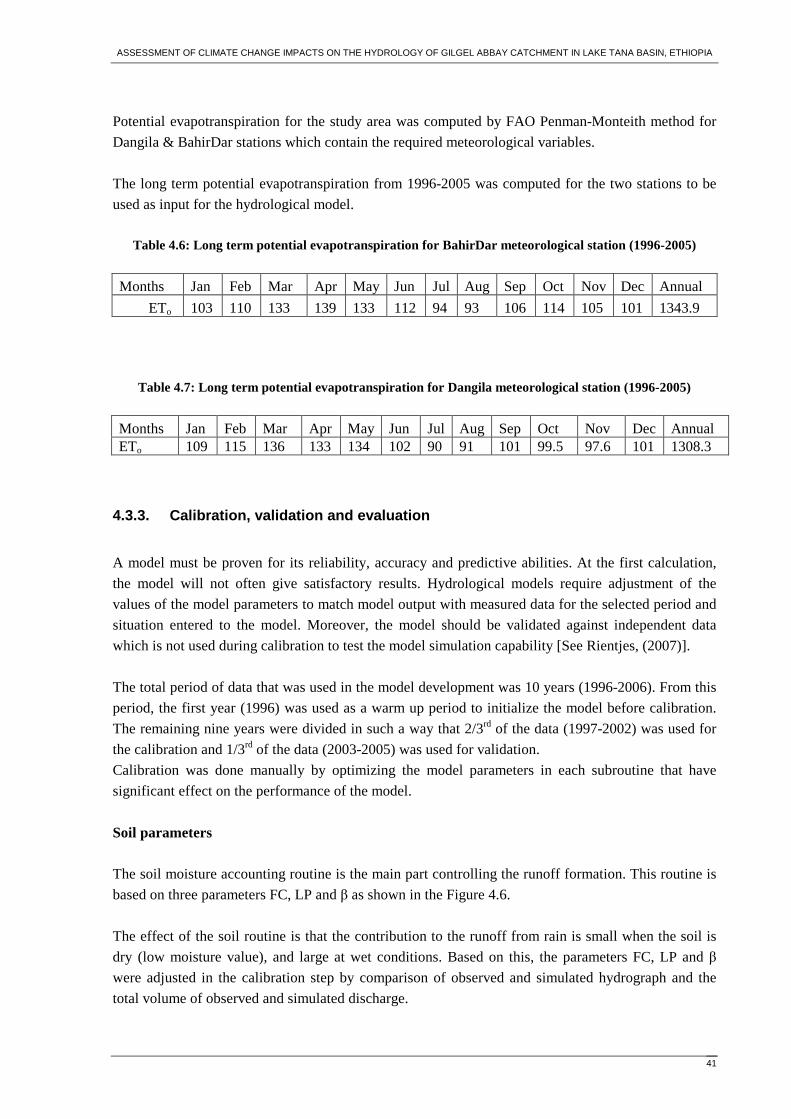
ASSESSMENT OF CLIMATE CHANGE IMPACTS ON THE HYDROLOGY OF GILGEL ABBAY CATCHMENT IN LAKE TANA BASIN, ETHIOPIA
41
Potential evapotranspiration for the study area was computed by FAO Penman-Monteith method for
Dangila & BahirDar stations which contain the required meteorological variables.
The long term potential evapotranspiration from 1996-2005 was computed for the two stations to be
used as input for the hydrological model.
Table 4.6: Long term potential evapotranspiration for BahirDar meteorological station (1996-2005)
Months Jan Feb Mar Apr May Jun Jul Aug Sep Oct Nov Dec Annual
ETo 103 110 133 139 133 112 94 93 106 114 105 101 1343.9
Table 4.7: Long term potential evapotranspiration for Dangila meteorological station (1996-2005)
Months Jan Feb Mar Apr May Jun Jul Aug Sep Oct Nov Dec Annual ETo 109 115 136 133 134 102 90 91 101 99.5 97.6 101 1308.3
4.3.3. Calibration, validation and evaluation
A model must be proven for its reliability, accuracy and predictive abilities. At the first calculation,
the model will not often give satisfactory results. Hydrological models require adjustment of the
values of the model parameters to match model output with measured data for the selected period and
situation entered to the model. Moreover, the model should be validated against independent data
which is not used during calibration to test the model simulation capability [See Rientjes, (2007)].
The total period of data that was used in the model development was 10 years (1996-2006). From this
period, the first year (1996) was used as a warm up period to initialize the model before calibration.
The remaining nine years were divided in such a way that 2/3rd of the data (1997-2002) was used for
the calibration and 1/3rd of the data (2003-2005) was used for validation.
Calibration was done manually by optimizing the model parameters in each subroutine that have
significant effect on the performance of the model.
Soil parameters The soil moisture accounting routine is the main part controlling the runoff formation. This routine is
based on three parameters FC, LP and β as shown in the Figure 4.6.
The effect of the soil routine is that the contribution to the runoff from rain is small when the soil is
dry (low moisture value), and large at wet conditions. Based on this, the parameters FC, LP and β
were adjusted in the calibration step by comparison of observed and simulated hydrograph and the
total volume of observed and simulated discharge.

ASSESSMENT OF CLIMATE CHANGE IMPACTS ON THE HYDROLOGY OF GILGEL ABBAY CATCHMENT IN LAKE TANA BASIN, ETHIOPIA
42
Figure 4.6: Relationship between parameter in soil routine (SMHI, 2006)
Where,
SM = computed soil moisture storage
∆P = contribution from rainfall
∆Q = contribution to the response function
FC = maximum soil moisture storage
β = empirical coefficient
E pot = potential evapotranspiration
Ea = computed actual evapotranspiration
LP = limit for potential evpotranspiration
Response parameter The runoff generation routine is the response function which transforms excess water from the soil
moisture zone to runoff. This routine consists of one non linear upper reservoir in the upper zone and
one linear reservoir in the lower zone. These two reservoirs are the origin of the quick and slow runoff
component of the hydrograph.
The outflow from the upper reservoir is described by a function corresponding to a continuously
increasing recession coefficient:
( )α1UZkoQ +∗= (6)
Where,
Qo = reservoir outflow upper reservoir (mm)
UZ = reservoir content upper reservoir (mm)
k = recession coefficient upper reservoir
The outflow from the lower linear reservoir is described by:
LZ4k1Q ∗= (7)
Where,
Q1 = reservoir outflow lower reservoir (mm)
LZ = reservoir content lower reservoir (mm)

ASSESSMENT OF CLIMATE CHANGE IMPACTS ON THE HYDROLOGY OF GILGEL ABBAY CATCHMENT IN LAKE TANA BASIN, ETHIOPIA
43
k4 = recession coefficient upper reservoir
Figure 4.7: The response routine
The main parameters in the response routine which require optimisation through calibration are k4,
per, khq, hq and α. These parameters govern to a large extent the model behaviour and define the
magnitude of the calculated discharge in time and influence the shape of the hydrograph rather than
the total volume.
hq is calculated using equation (8) for observed discharge and does not need calibration after it has
been calculated (SMHI, 2006).
( )
A
86.41/2
MHQMQqh
∗∗= (8)
Where,
MQ = Mean of observed discharge over the whole period (m3/s)
MHQ = Mean of annual peaks (m3/s)
A = Area (km2 )
hq for Gilgel Abbay Rivers becomes 3.3684 mm/day.
The baseflow is calibrated by examining observed and simulated hydrograph for the low flow period
using the parameter perc and k4. Perc was used to adjust the level of baseflow in which high perc
value increase the baseflow and vice versa. The recession of the baseflow is adjusted by k4. The peak
of the hydrograph was fine tuned by the parameter khq and α. A higher khq results in higher peaks
and a more dynamic response in the hydrograph.
After the calibration, the model was validated against independent data withheld from calibration.
Finally the model performance was evaluated for both calibration and validation in different ways
including:
1. By visually inspecting and comparing the calculated and observed hydrograph

ASSESSMENT OF CLIMATE CHANGE IMPACTS ON THE HYDROLOGY OF GILGEL ABBAY CATCHMENT IN LAKE TANA BASIN, ETHIOPIA
44
2. By calculating the explained variance R2
∑
∑ ∑=2)Qobs-(Qobs
2
Qobs)-(Qsim-2)Qobs - Qobs (2R (9)
Where,
Qobs = Observed discharge
Qsim = Simulated discharge
Qobs = Mean of observed discharge
This efficiency criterion was introduced by Nash and Sutcliffe and is commonly used in hydrological
modelling. If this value lies between 0.8 and 0.95 the performance of the model is very good.
3. By calculating the relative volume of error
100Qobs
Qsim)-(QobsR.V.E ∗
∑
∑= (10)
4.4. Hydrological impact of climate change
As discussed in section 4.1& 4.2 the model output of HadCM3 was used in this study to simulate the
climatic effect of increased atmospheric concentration of greenhouse gases and the climate model
output was downscaled to catchment scale using Statistical DownScaling Model (SDSM). Simulation
of streamflow corresponding to future climate change scenario was done using the HBV model which
was calibrated and validated as discussed in the previous section. The downscaled climate scenario
consists of maximum temperature; minimum temperature and precipitation together with an estimated
potential evapotranspiration were used as input to the model. The evapotanspiration was computed
based on the downscaled temperature.
The analysis of the simulated streamflow was carried out in three time horizons in future periods each
covering non overlapping 30 years. These period consists of 2020s (2011-2040); 2050s (2041-2070)
and 2080s (2071-2099). The same representation is also used in section 5 and 6 of the thesis.
In addition to climate model-based scenarios, incremental (synthetic) scenario was also used to
investigate a wide range of changes in climatic variables which in turn helps to test the system
sensitivity to climate.
The overall step that was used to investigate the hydrological impact of climate change was described
by the following simple conceptual framework.
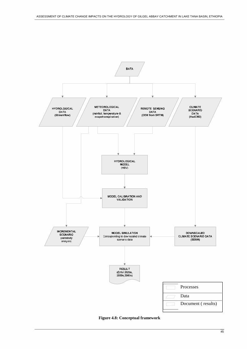
ASSESSMENT OF CLIMATE CHANGE IMPACTS ON THE HYDROLOGY OF GILGEL ABBAY CATCHMENT IN LAKE TANA BASIN, ETHIOPIA
45
Figure 4.8: Conceptual framework
Processes
Data
Document ( results)

ASSESSMENT OF CLIMATE CHANGE IMPACTS ON THE HYDROLOGY OF GILGEL ABBAY CATCHMENT IN LAKE TANA BASIN, ETHIOPIA
46

ASSESSMENT OF CLIMATE CHANGE IMPACTS ON THE HYDROLOGY OF GILGEL ABBAY CATCHMENT IN LAKE TANA BASIN, ETHIOPIA
47
5. RESULTS AND DISCUSSION
5.1. Downscaling the GCM output
5.1.1. Downscaling the GCM for the baseline period
One of the criteria commonly used in evaluating the performance of any useful downscaling method is
whether the historic (observed) condition can be replicated or not. It is therefore imperative that the
methods used for transferring the results of climate models to meteorological stations generate
precipitation and temperature time series that have the same statistical properties as observed
meteorological data that is used for hydrological modelling. Thus the HadCM3 was downscaled for
the baseline period for two emission scenarios (A2&B2) and the statistical properties (mean &
variance) of the downscaled data was compared with observed data. The IPCC recommends 1961-
1990 as climatological baseline period in impact assessment. Therefore this period was also used as
baseline period for this study. As discussed in the previous section the downscaling experiment was
conducted for minimum temperature, maximum temperature and precipitation based on the data from
BahirDar meteorological station which contain observed data for the specified period and the results
are discussed in section below.
(I) Minimum temperature
The monthly minimum temperature downscaled for A2 and B2 scenario in the baseline period is
shown in Figure 5.1
0
2
4
6
8
10
12
14
16
J F M A M J J A S O N DTime (month)
Tem
pera
ture
(o C
)
Observed Downscaled-HadCM3A2a Downscaled-HadCM3B2a
Figure 5.1: Observed and downscaled monthly mean minimum temperature for the baseline period (1961- 1990)

ASSESSMENT OF CLIMATE CHANGE IMPACTS ON THE HYDROLOGY OF GILGEL ABBAY CATCHMENT IN LAKE TANA BASIN, ETHIOPIA
48
The result of downscaling minimum temperature indicates that there is satisfactory agreement
between observed and simulated minimum temperature. As shown in Figure 5.2, the absolute model
error in estimate of the monthly minimum temperature is less than or equal to 0.3oC from January to
October and 0.4-0.5oC in the months of November and December. The model error in each month is
less than the projected temperature change in the future. Besides, the variability of observed monthly
minimum temperature is well preserved in the downscaled minimum temperature for most of the
months except small difference in the months of September.
0.0
0.1
0.2
0.3
0.4
0.5
J F M A M J J A S O N D
Time (month)
Mod
el e
rror
(o C
)
HadCM3A2a HadCM3B2a
Figure 5.2: Absolute model error in estimate of monthly minimum temperature
0
2
4
6
8
10
12
14
J F M A M J J A S O N D
Time (month)
Var
ianc
e (o C
2 )
Observed HadCM3A2a HadCM3B2a
Figure 5.3: Variance of observed and downscaled monthly minimum temperature

ASSESSMENT OF CLIMATE CHANGE IMPACTS ON THE HYDROLOGY OF GILGEL ABBAY CATCHMENT IN LAKE TANA BASIN, ETHIOPIA
49
(II) Maximum temperature The monthly maximum temperature downscaled for A2 and B2 scenario in the baseline period is
shown in Figure 5.4
0
5
10
15
20
25
30
35
J F M A M J J A S O N DTime (months)
Tem
pera
ture
(o C
)
Observed Downscaled-HadCM3A2a Downscaled-HadCM3B2a
Figure 5.4: Observed and downscaled monthly mean maximum temperature for the baseline period (1961-1990) The absolute model error in estimate of the mean maximum temperature is less than 0.6oC from
January to August and in October whereas the error becomes around 0.8oC in the months of
September and December.
00.10.20.30.40.50.60.70.80.9
J F M A M J J A S O N D
Time (month)
Mod
el e
rror
(o C
)
HadCM3A2a HadCM3B2a
Figure 5.5: Absolute model error in estimate of monthly maximum temperature
The variability of monthly maximum temperature of observed values is well preserved in the
downscaled value from July to December. From January to June the variance of observed value is
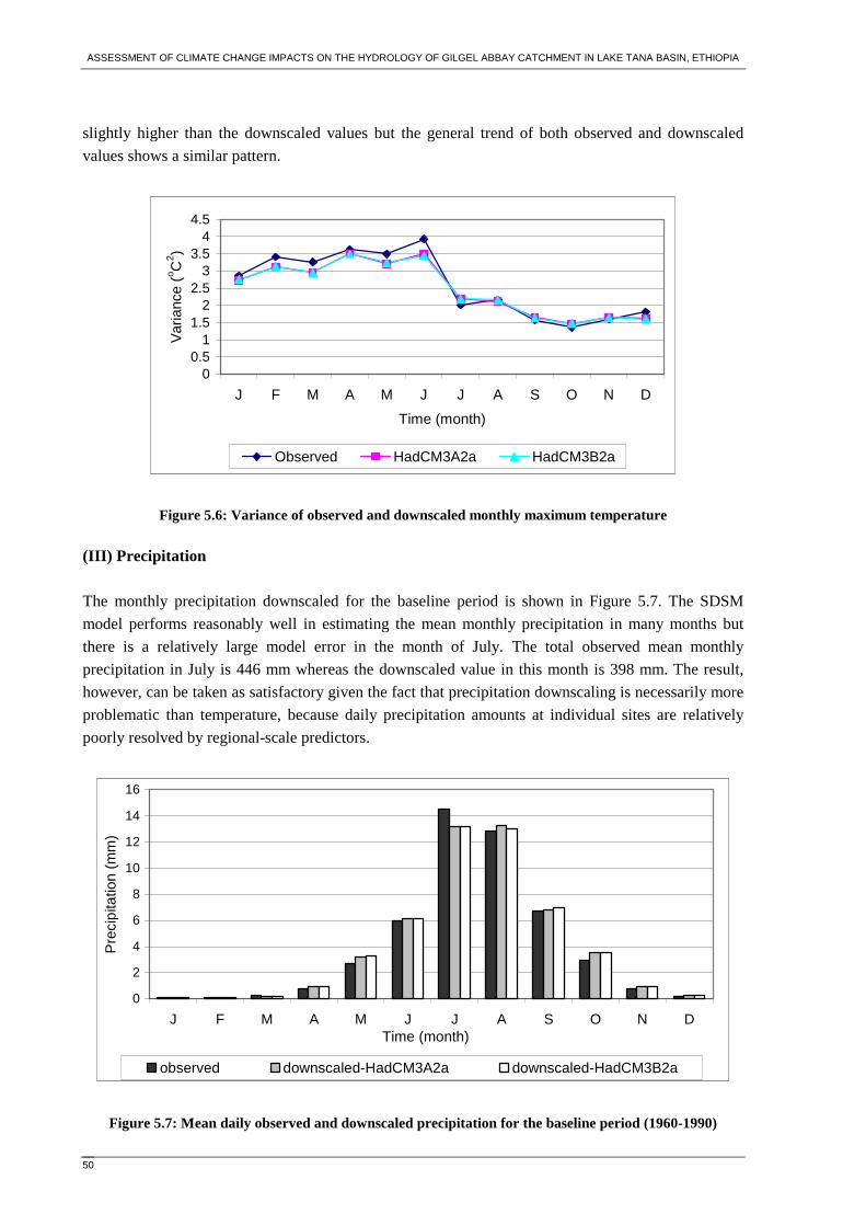
ASSESSMENT OF CLIMATE CHANGE IMPACTS ON THE HYDROLOGY OF GILGEL ABBAY CATCHMENT IN LAKE TANA BASIN, ETHIOPIA
50
slightly higher than the downscaled values but the general trend of both observed and downscaled
values shows a similar pattern.
00.5
11.5
22.5
33.5
44.5
J F M A M J J A S O N D
Time (month)
Var
ianc
e (o C
2 )
Observed HadCM3A2a HadCM3B2a
Figure 5.6: Variance of observed and downscaled monthly maximum temperature
(III) Precipitation The monthly precipitation downscaled for the baseline period is shown in Figure 5.7. The SDSM
model performs reasonably well in estimating the mean monthly precipitation in many months but
there is a relatively large model error in the month of July. The total observed mean monthly
precipitation in July is 446 mm whereas the downscaled value in this month is 398 mm. The result,
however, can be taken as satisfactory given the fact that precipitation downscaling is necessarily more
problematic than temperature, because daily precipitation amounts at individual sites are relatively
poorly resolved by regional-scale predictors.
0
2
4
6
8
10
12
14
16
J F M A M J J A S O N DTime (month)
Pre
cipi
tatio
n (m
m)
observed downscaled-HadCM3A2a downscaled-HadCM3B2a
Figure 5.7: Mean daily observed and downscaled precipitation for the baseline period (1960-1990)

ASSESSMENT OF CLIMATE CHANGE IMPACTS ON THE HYDROLOGY OF GILGEL ABBAY CATCHMENT IN LAKE TANA BASIN, ETHIOPIA
51
0
0.2
0.4
0.6
0.8
1
1.2
1.4
J F M A M J J A S O N D
Time (months)
Mod
el e
rror
(m
m)
HadCM3A2a HadCM3B2a
Figure 5.8: Absolute model error in estimates of the mean daily precipitation
0.0
100.0
200.0
300.0
400.0
500.0
J F M A M J J A S O N DTime (month)
Var
ianc
e (m
m2 )
Observed HadCM3A2a HadCM3B2a
Figure 5.9: Variance of observed and downscaled monthly mean precipitation
The variability of observed and downscaled precipitation shows good agreement in many months
however, the variance of observed precipitation is higher than the downscaled value in July and
August. Generally speaking the variance of observed and downscaled precipitation exhibits a similar
pattern i.e. an increase in variance of observed value is also reflected in the downscaled precipitation
and vice versa.
5.1.2. Downscaling the GCM for future scenario
The climate scenario for future period was developed from statistical downscaling using the GCM
predictor variables for the two emission scenarios for 100 years based on the mean of 20 ensembles
and the analysis was done based on three 30-year periods centred on the 2020s (2011-2040), 2050s
(2041-2070) and 2080s (2071-2099).

ASSESSMENT OF CLIMATE CHANGE IMPACTS ON THE HYDROLOGY OF GILGEL ABBAY CATCHMENT IN LAKE TANA BASIN, ETHIOPIA
52
(I) Minimum temperature The downscaled minimum temperature shows an increasing trend in all future time horizons for both
A2 and B2 scenarios. The average annual minimum temperature will be increased by 1oC in 2020s. In
2050s the increment will be 2.2oC and 1.7oC for A2 and B2 scenario respectively. For the 2080s
periods the average annual minimum temperature will be increased by 3.7oC and 2.7oC for A2 and B2
scenario respectively. The increment for A2 scenario is greater than B2 scenario because A2 scenario
represents a medium high scenario which produces more CO2 concentration than the B2 scenario
which represents a medium low scenario. The relative change of monthly minimum temperature
varies from month to month. The minimum relative change of temperature is observed in July where
the minimum temperature increased by 1.7oC and 1.2oC in 2080s for A2 and B2 scenario respectively
where as the maximum change of temperature is observed in April where the minimum temperature is
increased by 5.8oC and 4.3oC for A2 and B2 scenario respectively.
0.0
1.0
2.0
3.0
4.0
5.0
6.0
7.0
J F M A M J J A S O N D
Time (months)
Cha
nge
in te
mpe
ratu
re(o C
)
2020s 2050s 2080s
Figure 5.10: Change of downscaled monthly minimum temperature from the baseline period for HadCM3A2a
0.0
1.0
2.0
3.0
4.0
5.0
J F M A M J J A S O N D
Time (months)
chan
ge in
tem
pera
ture
(o C
)
2020s 2050s 2080s
Figure 5.11: Change of downscaled monthly minimum temperature from the baseline period for HadCM3B2a

ASSESSMENT OF CLIMATE CHANGE IMPACTS ON THE HYDROLOGY OF GILGEL ABBAY CATCHMENT IN LAKE TANA BASIN, ETHIOPIA
53
(II) Maximum temperature The downscaled maximum temperature scenario also indicates that there will be an increasing trend
for both A2 and B2 scenario. The projected temperature in 2020s indicates that maximum temperature
will rise by 0.6oC. In 2050s the increment will be 1.4oC and 1.1oC for A2 and B2 scenario
respectively. In 2080s the annual maximum temperature will be increased by 2.5oC and 1.8oC for A2
and B2 scenario respectively. The increment in maximum temperature is less than the minimum
temperature. The relative increment of maximum temperature from the baseline period for both
scenarios in future time horizon are shown in the Figures 5.12 and 5.13. The projected minimum and
maximum temperature in all future time horizons is within the range projected by IPCC which
indicate that the average temperature will be rises by 1.4-5.8oC towards the end of this century.
0.0
0.5
1.0
1.5
2.0
2.5
3.0
3.5
4.0
J F M A M J J A S O N DTime (month)
Cha
nge
in te
mpe
ratu
re (
o C)
2020s 2050s 2080s
Figure 5.12: Change in monthly maximum temperature between the baseline period and future for HadCM3A2a
0.0
0.5
1.0
1.5
2.0
2.5
3.0
3.5
J F M A M J J A S O N D
Time (month)
Cha
nge
in t
empe
ratu
re (
o C)
2020s 2050s 2080s
Figure 5.13: Change in monthly maximum temperature between the baseline period and future for HadCM3B2a

ASSESSMENT OF CLIMATE CHANGE IMPACTS ON THE HYDROLOGY OF GILGEL ABBAY CATCHMENT IN LAKE TANA BASIN, ETHIOPIA
54
(III) Precipitation Projection of rainfall did not manifest a systematic increase or decrease in all future time horizon
unlike that of maximum and minimum temperature which exhibits an increasing trend for both A2 and
B2 scenario in all future time horizon. The rainfall amount generally shows a decreasing trend in the
beginning of rainy season (May and June) and shows increasing trend towards the end of the rainy
reason (September and October) for both A2 & B2 scenario in all future time horizon. The rainfall
will experience a decrease of 18% and 11.2% in June from the baseline period by 2080s for A2 and
B2 scenario respectively where as the rainfall increase by 8.5% and 5.7% in September by 2080s for
A2 and B2 scenario respectively. The rainfall will also indicate a reduction in July and August from
the baseline period for A2 scenario in all future time horizons however, for B2 scenario there is also
indication of increment in some future time horizon. In the main rainy season (June-September) the
rainfall exhibits relative decrease from the baseline period for A2 scenario in all future time horizons
where as B2 scenario indicates a decrease by 2020s and a slight increment by 2050s and 2080s. The
mean annual rainfall variation is not significant compared to the monthly variation. The mean annual
rainfall will indicate a decrease in 2020s followed by a slight increase in 2050s and 2080s.
02468
10121416
J F M A M J J A S O N DTime (month)
Pre
cipi
tatio
n (m
m)
observed downscaled-HadCM3A2a downscaled-HadCM3B2a
Figure 5.14: Mean daily precipitation downscaled from HadCM3A2a
02468
10121416
J F M A M J J A S O N DTime (month)
Pre
cipi
tatio
n (m
m)
current 2020s 2050s 2080s
Figure 5.15: Mean daily precipitation downscaled from HadCM3B2a

ASSESSMENT OF CLIMATE CHANGE IMPACTS ON THE HYDROLOGY OF GILGEL ABBAY CATCHMENT IN LAKE TANA BASIN, ETHIOPIA
55
The mean monthly rainfall distribution downscaled from SDSM shows a similar pattern with work of
deBoor,(2007) which describes the impact of climate change on rainfall pattern in Ethiopian highland.
As he indicated in his work the mean monthly rainfall decrease in May, June and July and increase in
September, October and November with respect to the baseline period (Figure 5.16).A similar trend is
also observed in the downscaled precipitation for most future time slices as indicated in Figure 5.14
and 5.15.
Present climate (1951-2000)
Future climate (2051-2100)
Figure 5.16: Mean daily precipitation for Ethiopian highland between the present and future
(deBoer, 2007)
As described in the IPCC Third Assessment Report (McCarthy et al., 2001), the projected future
changes in mean seasonal rainfall in Africa are less well defined. The diversity of African climates,
high rainfall variability, and a very sparse observational network make the predictions of future
climate change difficult at the sub regional and local scales. Under intermediate warming scenarios,
rainfall is predicted to increase in December-February and decrease in June-August in parts of East
Africa. With a more rapid global warming scenario, large areas of Africa would experience changes in
December-February or June-August rainfall that exceed natural variability. With reference to this
study rainfall will also experience a reduction in June-August for most part of the future time horizons
however, the rainfall variation in December-February is not significant because these are the driest
month which contribute less than 1% of the annual rainfall in the study area. Conway also indicates
that with respect to the future climate in the Nile basin there is high confidence that the temperature
will rise, leading to an increased evaporation. However, there is much less certainty about future
rainfall because of the low convergence in climate model projection in the key headwater regions of
the Nile (Conway, 2005). The same paper states that there is large inter-model difference in the detail
of rainfall changes over Ethiopia using the results from seven recent climate model experiments.
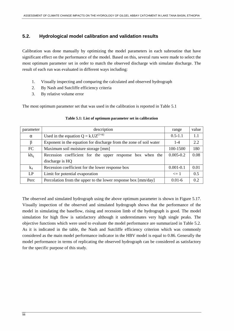
ASSESSMENT OF CLIMATE CHANGE IMPACTS ON THE HYDROLOGY OF GILGEL ABBAY CATCHMENT IN LAKE TANA BASIN, ETHIOPIA
56
5.2. Hydrological model calibration and validation results
Calibration was done manually by optimizing the model parameters in each subroutine that have
significant effect on the performance of the model. Based on this, several runs were made to select the
most optimum parameter set in order to match the observed discharge with simulate discharge. The
result of each run was evaluated in different ways including:
1. Visually inspecting and comparing the calculated and observed hydrograph
2. By Nash and Sutcliffe efficiency criteria
3. By relative volume error
The most optimum parameter set that was used in the calibration is reported in Table 5.1
Table 5.1: List of optimum parameter set in calibration
parameter description range value
α Used in the equation Q = k.UZ(1+α) 0.5-1.1 1.1
β Exponent in the equation for discharge from the zone of soil water 1-4 2.2
FC Maximum soil moisture storage [mm] 100-1500 180
khq Recession coefficient for the upper response box when the
discharge is HQ
0.005-0.2 0.08
k4 Recession coefficient for the lower response box 0.001-0.1 0.01
LP Limit for potential evaporation <= 1 0.5
Perc Percolation from the upper to the lower response box [mm/day] 0.01-6 0.2
The observed and simulated hydrograph using the above optimum parameter is shown in Figure 5.17.
Visually inspection of the observed and simulated hydrograph shows that the performance of the
model in simulating the baseflow, rising and recession limb of the hydrograph is good. The model
simulation for high flow is satisfactory although it underestimates very high single peaks. The
objective functions which were used to evaluate the model performance are summarized in Table 5.2.
As it is indicated in the table, the Nash and Sutcliffe efficiency criterion which was commonly
considered as the main model performance indicator in the HBV model is equal to 0.86. Generally the
model performance in terms of replicating the observed hydrograph can be considered as satisfactory
for the specific purpose of this study.

ASSESSMENT OF CLIMATE CHANGE IMPACTS ON THE HYDROLOGY OF GILGEL ABBAY CATCHMENT IN LAKE TANA BASIN, ETHIOPIA
57
0
50
100
150
200
250
300
350
400
45001
/01/
1997
01/0
5/19
97
01/0
9/19
97
01/0
1/19
98
01/0
5/19
98
01/0
9/19
98
01/0
1/19
99
01/0
5/19
99
01/0
9/19
99
01/0
1/20
00
01/0
5/20
00
01/0
9/20
00
01/0
1/20
01
01/0
5/20
01
01/0
9/20
01
01/0
1/20
02
01/0
5/20
02
01/0
9/20
02
Time (day,month,year)
Dis
char
ge (
m3 /s
)
observed simulated
Figure 5.17: Daily observed and simulated hydrograph during calibration period
Table 5.2: List of objective function and its value obtained during calibration
Objective function Formula value
Nash and Sutcliffe
efficiency coefficient, 2R
∑
∑ ∑=2)Qobs-(Qobs
2
Qobs)-(Qsim-2)Qobs - Qobs (2R 0.86
2logR
∑
∑ ∑=2
222
)logQobs-(logQobs
logQobs)-(logQsim-)logQobs - Qobs (loglogR
0.87
Correlation
coefficient, r ∑ −∑ −
∑ −−2)Qsim(Qsim2)Qobs(Qobs
)Qsim)(QsimQobs(QobsCorr
0.92
Relative Volume
error, R.V.E (%) 100
Qobs
Qsim)-(QobsR.V.E ∗
∑
∑= -0.13
The model result as shown in Figure 5.18 indicates that the observed and simulated hydrograph do
have better agreement in mean monthly flow compared to daily flow.
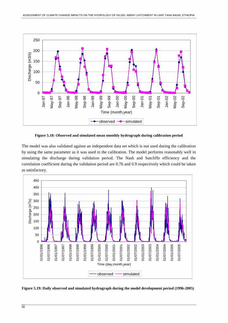
ASSESSMENT OF CLIMATE CHANGE IMPACTS ON THE HYDROLOGY OF GILGEL ABBAY CATCHMENT IN LAKE TANA BASIN, ETHIOPIA
58
0
50
100
150
200
250Ja
n-97
May
-97
Sep
-97
Jan-
98
May
-98
Sep
-98
Jan-
99
May
-99
Sep
-99
Jan-
00
May
-00
Sep
-00
Jan-
01
May
-01
Sep
-01
Jan-
02
May
-02
Sep
-02
Time (month,year)
Dis
char
ge (
m3/
s)
observed simulated
Figure 5.18: Observed and simulated mean monthly hydrograph during calibration period
The model was also validated against an independent data set which is not used during the calibration
by using the same parameter as it was used in the calibration. The model performs reasonably well in
simulating the discharge during validation period. The Nash and Sutcliffe efficiency and the
correlation coefficient during the validation period are 0.76 and 0.9 respectively which could be taken
as satisfactory.
0
50
100
150
200
250
300
350
400
450
01/0
1/19
96
01/0
7/19
96
01/0
1/19
97
01/0
7/19
97
01/0
1/19
98
01/0
7/19
98
01/0
1/19
99
01/0
7/19
99
01/0
1/20
00
01/0
7/20
00
01/0
1/20
01
01/0
7/20
01
01/0
1/20
02
01/0
7/20
02
01/0
1/20
03
01/0
7/20
03
01/0
1/20
04
01/0
7/20
04
01/0
1/20
05
01/0
7/20
05
Time (day,month,year)
Dis
char
ge (
m3 /s
)
observed simulated
Figure 5.19: Daily observed and simulated hydrograph during the model development period (1996-2005)

ASSESSMENT OF CLIMATE CHANGE IMPACTS ON THE HYDROLOGY OF GILGEL ABBAY CATCHMENT IN LAKE TANA BASIN, ETHIOPIA
59
5.3. Hydrological impact of future climate change scenario
The ultimate objective of the downscaling is to generate an estimate of meteorological variables
corresponding to a given scenario of the future climate so that these meteorological variables will be
used as a basis for hydrological impact assessment. Therefore, after calibrating the hydrological
models with the historical record, the next step is the simulation of river flows in the catchment by
using the downscaled precipitation and temperature and evapotranspiration as input to hydrological
models. The evapotranspiration is computed based on the downscaled minimum and maximum
temperature for each time horizon. Subsequently the hydrological model was used to identify possible
trends in the simulated river flow. Based on this, hydrological impact of the Gilgel Abbay River is
analyzed using HBV models with respect to three 30 years period centred on 2020s, 2050s and 2080s.
The present condition in the hydrological model is represented by taking the average of the longest
possible records available in study area. These include at least ten years data for all station used in the
analysis.
The simulation results for three future time horizons are summarized in Table 5.3 and Figures 5.20
and 5.21. As it is shown in table the variation in mean annual runoff is moderate. The mean annual
runoff will be reduced by 2.6% and 2.9% in 2080s for A2 and B2 scenario respectively. However,
there is significant variation in the seasonal and monthly flow. In the main rainy season (June-Sep) the
runoff will be reduced by 11.6% and 10.1% in 2080s for A2 and B2 scenario respectively. With
respect to individual months, there will be large reduction in June where the mean monthly flow will
reduced by 66% and 59% in 2080s for A2 and B2 scenario respectively. July also exhibit a reduction
in mean monthly flow where the flow will be reduced by 20% and 16% in the 2080s for A2 and B2
scenario respectively. In August with the exception of B2 scenario at the 2050s, there is reduction in
mean monthly flow as well. The mean monthly flow of the river will start to increase afterwards. In
September there will be mixed sign where the flow will start to decrease in 2020s and increase in
2050s and 2080s for both scenarios. The mean monthly flow of October will be increased by 33% and
15% in 2080s for both A2 and B2 scenario in all future time horizons. There will also be a reduction
in November for both A2 and B2 scenario in all future time horizons.
Table 5.3: Average increase/decrease of runoff (%) from the present condition
Time
A2-2020 A2-2050 A2-2080 B2-2020 B2-2050 B2-2080
Seasonal runoff (Jun-Sep) -11.6 -3.5 -12.2 -13.3 -1.4 -10.1
Annual runoff -5.4 0.2 -2.6 -6.8 0.4 -2.9
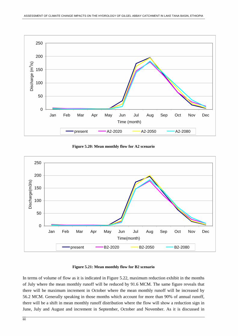
ASSESSMENT OF CLIMATE CHANGE IMPACTS ON THE HYDROLOGY OF GILGEL ABBAY CATCHMENT IN LAKE TANA BASIN, ETHIOPIA
60
0
50
100
150
200
250
Jan Feb Mar Apr May Jun Jul Aug Sep Oct Nov Dec
Time (month)
Dis
char
ge (
m3 /s
)
present A2-2020 A2-2050 A2-2080
Figure 5.20: Mean monthly flow for A2 scenario
0
50
100
150
200
250
Jan Feb Mar Apr May Jun Jul Aug Sep Oct Nov Dec
Time(month)
Dis
char
ge(m
3/s)
present B2-2020 B2-2050 B2-2080
Figure 5.21: Mean monthly flow for B2 scenario
In terms of volume of flow as it is indicated in Figure 5.22, maximum reduction exhibit in the months
of July where the mean monthly runoff will be reduced by 91.6 MCM. The same figure reveals that
there will be maximum increment in October where the mean monthly runoff will be increased by
56.2 MCM. Generally speaking in those months which account for more than 90% of annual runoff,
there will be a shift in mean monthly runoff distribution where the flow will show a reduction sign in
June, July and August and increment in September, October and November. As it is discussed in
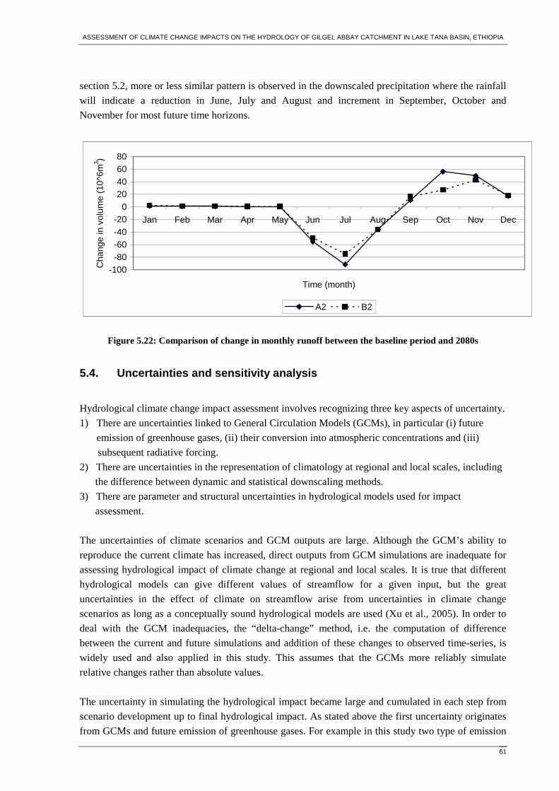
ASSESSMENT OF CLIMATE CHANGE IMPACTS ON THE HYDROLOGY OF GILGEL ABBAY CATCHMENT IN LAKE TANA BASIN, ETHIOPIA
61
section 5.2, more or less similar pattern is observed in the downscaled precipitation where the rainfall
will indicate a reduction in June, July and August and increment in September, October and
November for most future time horizons.
-100-80-60-40-20
020406080
Jan Feb Mar Apr May Jun Jul Aug Sep Oct Nov Dec
Time (month)
Cha
nge
in v
olum
e (1
0^6m
3 )
A2 B2
Figure 5.22: Comparison of change in monthly runoff between the baseline period and 2080s
5.4. Uncertainties and sensitivity analysis
Hydrological climate change impact assessment involves recognizing three key aspects of uncertainty.
1) There are uncertainties linked to General Circulation Models (GCMs), in particular (i) future
emission of greenhouse gases, (ii) their conversion into atmospheric concentrations and (iii)
subsequent radiative forcing.
2) There are uncertainties in the representation of climatology at regional and local scales, including
the difference between dynamic and statistical downscaling methods.
3) There are parameter and structural uncertainties in hydrological models used for impact
assessment.
The uncertainties of climate scenarios and GCM outputs are large. Although the GCM’s ability to
reproduce the current climate has increased, direct outputs from GCM simulations are inadequate for
assessing hydrological impact of climate change at regional and local scales. It is true that different
hydrological models can give different values of streamflow for a given input, but the great
uncertainties in the effect of climate on streamflow arise from uncertainties in climate change
scenarios as long as a conceptually sound hydrological models are used (Xu et al., 2005). In order to
deal with the GCM inadequacies, the “delta-change” method, i.e. the computation of difference
between the current and future simulations and addition of these changes to observed time-series, is
widely used and also applied in this study. This assumes that the GCMs more reliably simulate
relative changes rather than absolute values.
The uncertainty in simulating the hydrological impact became large and cumulated in each step from
scenario development up to final hydrological impact. As stated above the first uncertainty originates
from GCMs and future emission of greenhouse gases. For example in this study two type of emission
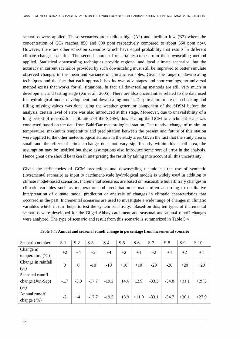
ASSESSMENT OF CLIMATE CHANGE IMPACTS ON THE HYDROLOGY OF GILGEL ABBAY CATCHMENT IN LAKE TANA BASIN, ETHIOPIA
62
scenarios were applied. These scenarios are medium high (A2) and medium low (B2) where the
concentration of CO2 reaches 850 and 600 ppm respectively compared to about 360 ppm now.
However, there are other emission scenarios which have equal probability that results in different
climate change scenarios. The second source of uncertainty comes from the downscaling method
applied. Statistical downscaling techniques provide regional and local climate scenarios, but the
accuracy in current scenarios provided by such downscaling must still be improved to better simulate
observed changes in the mean and variance of climatic variables. Given the range of downscaling
techniques and the fact that each approach has its own advantages and shortcomings, no universal
method exists that works for all situations. In fact all downscaling methods are still very much in
development and testing stage (Xu et al., 2005). There are also uncertainties related to the data used
for hydrological model development and downscaling model. Despite appropriate data checking and
filling missing values was done using the weather generator component of the SDSM before the
analysis, certain level of error was also introduced at this stage. Moreover, due to unavailability of a
long period of records for calibration of the SDSM, downscaling the GCM to catchment scale was
conducted based on the data from BahirDar meteorological station. The relative change of minimum
temperature, maximum temperature and precipitation between the present and future of this station
were applied to the other meteorological stations in the study area. Given the fact that the study area is
small and the effect of climate change does not vary significantly within this small area, the
assumption may be justified but these assumptions also introduce some sort of error in the analysis.
Hence great care should be taken in interpreting the result by taking into account all this uncertainty.
Given the deficiencies of GCM predictions and downscaling techniques, the use of synthetic
(incremental scenario) as input to catchment-scale hydrological models is widely used in addition to
climate model-based scenarios. Incremental scenarios are based on reasonable but arbitrary changes in
climatic variables such as temperature and precipitation is made often according to qualitative
interpretation of climate model prediction or analysis of changes in climatic characteristics that
occurred in the past. Incremental scenarios are used to investigate a wide range of changes in climatic
variables which in turn helps to test the system sensitivity. Based on this, ten types of incremental
scenarios were developed for the Gilgel Abbay catchment and seasonal and annual runoff changes
were analyzed. The type of scenario and result from this scenario is summarized in Table 5.4
Table 5.4: Annual and seasonal runoff change in percentage from incremental scenario
Scenario number S-1 S-2 S-3 S-4 S-5 S-6 S-7 S-8 S-9 S-10
Change in
temperature (oC) +2 +4 +2 +4 +2 +4 +2 +4 +2 +4
Change in rainfall
(%) 0 0 -10 -10 +10 +10 -20 -20 +20 +20
Seasonal runoff
change (Jun-Sep)
(%)
-1.7 -3.3 -17.7 -19.2 +14.6 12.9 -33.3 -34.8 +31.1 +29.3
Annual runoff
change ( %) -2 -4 -17.7 -19.5 +13.9 +11.9 -33.1 -34.7 +30.1 +27.9

ASSESSMENT OF CLIMATE CHANGE IMPACTS ON THE HYDROLOGY OF GILGEL ABBAY CATCHMENT IN LAKE TANA BASIN, ETHIOPIA
63
As it is shown in the table an increase in temperature of 2oC without rainfall change, decreases the
seasonal and annual runoff by 1.7% and 2% respectively. If the change in temperature is 4oC, the
seasonal and annual runoff would be decreased by 3.3% and 4% respectively. However, if the
increase in 2oC temperature will occur simultaneously with a rainfall reduction of 10%, the seasonal
and annual runoff will be decreased by 17.7%. If the reduction of rainfall is 20% and the temperature
will rise by 2oC, the seasonal and annual runoff will be reduced by 33%. From this analysis it is
possible to conclude that the Gilgel Abbay catchment is sensitive to climate change and it is more
sensitive to change in rainfall than change in temperature.

ASSESSMENT OF CLIMATE CHANGE IMPACTS ON THE HYDROLOGY OF GILGEL ABBAY CATCHMENT IN LAKE TANA BASIN, ETHIOPIA
64
ASSESSMENT OF CLIMATE CHANGE IMPACTS ON THE HYDROLOGY OF GILGEL ABBAY CATCHMENT IN LAKE TANA BASIN, ETHIOPIA
65
6. CONCLUSION AND RECOMMENDATION
The tremendous importance of water in both society and nature underscores the necessity of
understanding how a change in global climate could affect the availability and reliability of water
resources at a catchment scale. However, this is complicated by the fact that the climate change
information required for impact studies is of a spatial scale much finer than that provided by General
Circulation Models (GCMs). This mismatch between the two processes is partly resolved by
downscaling techniques even though the procedure of downscaling process also introduces some sort
of uncertainty. The problem was exacerbated by the lack of good quality data for a significantly long
period for the study area. Despite this, maximum effort was made to investigate the likely future of
hydrological impact of climate change and the following conclusion and recommendation are drawn
from this study.
6.1. Conclusion
� The results from the applied statistical downscaling model indicate that both the minimum
and maximum temperature show an increasing trend in all future time horizons for both A2
and B2 scenarios. The average annual minimum temperature will be increased by 3.7oC and
2.7oC for A2 and B2 scenario respectively towards the end of this century. The maximum
temperature will also increased by 2.5oC and 1.8oC for A2 and B2 scenario respectively
within the same time period. Climate change scenarios for Africa, based on the results from
several General Circulation Models using the data collated by the Intergovernmental Panel on
Climate Change Data Distribution Centre (IPCC-DDC) indicate that future warming across
Africa with ranges from 2oC (low scenario) to 5oC (high scenario) by 2100. Therefore the
result obtained from SDSM lies within the range of IPCC recommendations.
� The result of downscaled precipitation reveals that precipitation does not manifest a
systematic increase or decrease in all future time horizons for both A2 and B2 scenarios
unlike that of minimum and maximum temperature. However, in the main rainy season which
accounts 75-90% of annual rainfall of the area, the mean monthly rainfall indicates a
decreasing trend in the beginning of the rainy season (May & June) and an increasing trend
towards the end of the rainy season (September & October) for both A2 and B2 scenarios in
all future time horizons. Maximum reduction will be observed in June where the mean
monthly rainfall will be reduced by 18% and 11.2% in 2080s from the baseline period for A2
and B2 scenario respectively. A maximum increment will be observed in September where
the mean monthly rainfall will be reduced by 8.5% and 5.7% in 2080s for A2 and B2
scenarios respectively.
� The result of hydrological model calibration and validation indicates that the HBV model
simulates the runoff considerably good for the study area. The model performance criterion
ASSESSMENT OF CLIMATE CHANGE IMPACTS ON THE HYDROLOGY OF GILGEL ABBAY CATCHMENT IN LAKE TANA BASIN, ETHIOPIA
66
which is used to evaluate the model result indicates that the Nash and Sutcliffe efficiency
criteria (R2) are 0.86 and 0.76 during calibration and validation period respectively.
� The hydrological impact of future change scenarios indicates that there will be high seasonal
and monthly variation of runoff compared to the annual variation. In the main rainy season
(June-September) the runoff volume will reduce by 11.6% and 10.1% for A2 and B2 scenario
respectively in 2080s. The mean annual runoff will reduce by 2.6% and 2.9% for A2 and B2
scenario respectively within the same period.
� Results from synthetic (incremental) scenarios indicate that the catchment is sensitive to
climate change especially to change in rainfall. An increase of 2oC temperature without
changes in rainfall decreases the seasonal and annual runoff by 1.7% and 2%. However, if
change in temperature is accompanied by 20% rainfall reduction, seasonal and annual runoff
will be reduced by 33%.
� With respect to the past there is an increasing trend of both maximum and minimum
temperature which leads to an increase in evapotranspiration. The analysis of runoff of Gilgel
Abbay from 1973-2005 indicates that there is decreasing trend of the annual runoff. However,
it is difficult to be conclusive based on this limited analysis whether the changes are ascribed
to a significant greenhouse-induced climate changes or other changes such as land use in the
catchment.
6.2. Recommendation
� There are many sources of uncertainty in the hydrological impact scenarios that are in the
climate modelling, the method used for transferring the climate signal to meteorological
stations, and in the hydrological modelling. The model simulations have not considered land
use changes explicitly although, it is likely that changes in land use may interact with climate
leading to different projections of future hydrological conditions. Therefore the result of this
study should be taken with care and be considered as indication of likely future changes rather
than an actual prediction.
� The outcome of this study is based on single GCMs and two emission scenarios. However, it
is often recommended to apply different GCMs and emission scenarios so as to make
comparison between different models as well as to explore a wide range of climate change
scenarios that would result in different hydrological impacts. Hence this work should be
extended in the future by including different GCMs and emission scenarios.
� The GCMs was downscaled to catchment scale using the Statistical DownScaling Model
(SDSM) which is a regression based model. There also other downscaling methods such as
stochastic weather generators (for instance LAR-WG) and weather typing schemes which are
commonly applied in impact assessments. However, it not yet clear which methods gives the
most reliable estimate for future climate. In fact all downscaling methods are still very much

ASSESSMENT OF CLIMATE CHANGE IMPACTS ON THE HYDROLOGY OF GILGEL ABBAY CATCHMENT IN LAKE TANA BASIN, ETHIOPIA
67
in development and testing stage (Xu et al., 2005). Therefore other downscaling models
should also be tested to allow assessments based on the result from different downscaling
models.
� Water resources are inextricably linked with climate, so the prospect of global climate change
has serious implications for water resources. As water resources stresses become acute in
future as a result of a combination of climate impacts and escalating human demand, there
will be intensifying conflicts between human and environmental demands on water resources.
Therefore there is a need to minimize the sensitivity to climate change. One way to minimize
this risk is to make the economy more diversified, and agricultural technology should
optimize water usage through efficient irrigation and crop development. Moreover, research
activities should be intensified in this area in order to explore the impact of climate change on
various sectors including water resource by including recent findings in this area.

ASSESSMENT OF CLIMATE CHANGE IMPACTS ON THE HYDROLOGY OF GILGEL ABBAY CATCHMENT IN LAKE TANA BASIN, ETHIOPIA
68

ASSESSMENT OF CLIMATE CHANGE IMPACTS ON THE HYDROLOGY OF GILGEL ABBAY CATCHMENT IN LAKE TANA BASIN, ETHIOPIA
69
REFERENCE
Aerts, J. C. J. H. & Droogers, P. (2004). Climate change in contrasting river basins: adaptation strategies for water, food and environment. Wallingford: CABI.
Allen, R. G., Pereria, L. S., Raes, D. & Smith, M. (1998). Crop Evapotranspiration:Guidelines for computing crop water requirements. FAO, Rome.
Booij, M. J. (2005). Impact of climate change on river flooding assessed with different spatial model resolutions. Journal of Hydrology, 303(1-4), 176-198.
Carter, T. R. (2007). General Guidelines on the use of scenario data for Climate Impact and Adaptation Assessment. Finnish Environmental Institute, Helsinki, Finland.
Conway, D. (2005). From headwater tributaries to international river: Observing and adapting to climate variability and change in the Nile basin. Global Environmental Change, 15, 99–114.
Dawson, C. W. & Wilby, R. L. (2007). Statistical Downscaling Model SDSM, version 4.1. Department of Geography, Lancaster University, UK.
deBoer, B. (2007). Climate change and impacts on the extreme rainfall over the Blue Nile region. KNMI, Royal Netherlands Meteorological Institute, De Bilt, Netherlands.
Dibike, Y. B. & Coulibaly, P. (2004). Downscaling of Global Climate Model Output for Flood Frequency Analysis in the Saguenay River System. Project no. S02-15-01, Department of Civil Engineering, McMaster University, Canada.
Dibike, Y. B. & Coulibaly, P. (2005). Hydrologic impact of climate change in the Saguenay watershed: comparison of downscaling methods and hydrologic models. Journal of Hydrology, 307(1-4), 145-163.
Houghton, J. T. (2001). Climate change 2001: the scientific basis: contribution of working group I to the third assessment report of the intergovernmental panel on climate change (Houghton, J. T.,Ed.). Cambridge: Cambridge University Press.
http://www.cics.uvic.ca/scenarios/sdsm/select.cgi. Canadian Climate Impacts Scenarios (CCIS) project.
http://www.ipcc-data.org/index.html. (2007). The Intergovernmental Panel on Climate Change Data Distribution Centre, IPCC-DDC.
Jenkins, G. (2005). Climate change and the greenhouse effect. Hadley Centre, Met Office, UK. Leavesley, G. H., Wilby, R. L. & Hay, L. E. (1999). A comparison of downscaled and raw GCM
output: implications for climate change scenarios in the San Juan River basin, Colorado. Journal of Hydrology, 225(1-2), 67-91.
Lindstrom, G., Johansson, B., Persson, M., Gardelin, M. & Bergstrom, S. (1997). Development and test of the distributed HBV-96 hydrological model. Journal of Hydrology, 201 272-288.
McCarthy, J. J., Canziani, O. F., Leary, N. A., Dokken, D. J. & White, K. S. (2001). Climate Change 2001: Impacts, Adaptation, and Vulnerability Contribution of Working Group II to the Third Assessment Report of the Intergovernmental Panel on Climate Change.
NMSA. (2001). Initial National Communication of Ethiopia to the United Nations Framework Convention on Climate Change (UNFCCC). National Meteorological Services Agency, Addis Ababa, Ethiopia.
Rientjies, T. (2007). Modelling in Hydrology, ITC lecture books. 233. Seibert, J. (2002). HBV light: version 2 user's manual. Department of Earth Sciences, Hydrology,
Uppsala University, Sweden.

ASSESSMENT OF CLIMATE CHANGE IMPACTS ON THE HYDROLOGY OF GILGEL ABBAY CATCHMENT IN LAKE TANA BASIN, ETHIOPIA
70
Semenov, M. A. (2002). LARS-WG A Stochastic Weather Generator for Use in Climate Impact
Studies: User Manual Version 3.0. Rothamsted Research, Harpenden, Hertfordshire, AL5 2JQ, UK.
SMEC. (2007). Hydrological study of the Tana and Beles sub basin -Inception report. SMEC International pty Ltd, Addis Ababa, Ethiopia.
SMHI. (2006). Integrated Hydrological Modelling System: Manual Version 5.10. . Tessema, S. M. (2006). Assessment of temporal hydrological variations due to land use changes
using remote sensing/GIS: A case study of Lake Tana Basin. Msc Thesis, KTH/ Department of Land Water Resources Engineering, Stockholm, Sweden. .
Wilby, L. R., Zorita, E., Timbal, B., Whetton, P., Mearns, L. O. & Charles, S. P. ( 2004). Guidelines for use of Climate Scenario Developed from Statistical Downscaling Methods. Environmental Agency of England and Wales, UK.
Xu, C. Y. (1999). From GCMs to river flow: a review of downscaling methods and hydrologic modelling approaches. Progress in Physical Geography, 23(2), 229-249.
Xu, C. Y., Widen, E. & Halldin, S. (2005). Modelling Hydrological Consequences of Climate Change—Progress and Challenges. Advances in Atmospheric Sciences 22 (6), 789–797.
ASSESSMENT OF CLIMATE CHANGE IMPACTS ON THE HYDROLOGY OF GILGEL ABBAY CATCHMENT IN LAKE TANA BASIN, ETHIOPIA
71
ANNEX
Annex A Definition of common terms and acronymys
Projection The term “projection” is used in two senses in the climate change literature. In
general usage, a projection can be regarded as any description of the future and the pathway
leading to it. However, a more specific interpretation has been attached to the term “climate
projection” by the IPCC when referring to model-derived of future climate.
Forecast/ prediction When a projection is designated “most likely” it becomes a forecast or
prediction. A forecast is often obtained using physically- based models, possibly a set of these,
outputs of which can enable some level of confidence to be attached to projections.
Scenario A scenario is a coherent, internally consistent and plausible description of a possible
future state of the world. It is not a forecast; rather, each scenario is one alternative image of how
the future can unfold. A projection may serve as the raw material for a scenario but scenarios
often require additional information (e.g. about the baseline conditions). A set of scenarios is
often adopted to reflect, as well as possible, the range of uncertainty in the projection. Other
terms that have been used as synonyms for scenario are “characterisation”, “storyline” and
“construction”.
Baseline/ Reference A baseline (or reference) is any datum against which change is measured. It
might be a “current baseline”, in which case it represents observable, present day condition. It
might be also a “future baseline”, which is a projected set of conditions excluding the driving
factor of interest. Alternative interpretations of the reference conditions can give rise to multiple
baselines.
IPCC Intergovernmental Panel on Climate Change
GCM General Circulation Model
AOGCM Coupled Atmospheric-Ocean General Circulation Model
SDSM Statistical DownScaling Models
IPCC-DDC Data Distribution centre of Intergovernmental Panel on Climate Change
HadCM3 Hadley Centre for Climate Prediction and Research, UK
SRES Special Report on Emission Scenario
NCEP National Centre for Environmental Prediction
In this thesis the period 2020s represent period from 2011-2040, 2050s covers 2041-2070 and
2080s represent 2071-2099.

ASSESSMENT OF CLIMATE CHANGE IMPACTS ON THE HYDROLOGY OF GILGEL ABBAY CATCHMENT IN LAKE TANA BASIN, ETHIOPIA
72
Annex B Elevation and vegetation zone of the subbasins
Subbasin-one Elevation Landcover Npix Km^2 percentage 2130 * 1 Field 4737 38.37 6.8 2130 * 1 forest 190 1.54 0.3 2330 * 1 Field 21925 177.59 31.4 2330 * 1 forest 1843 14.93 2.6 2530 * 1 Field 17929 145.22 25.7 2530 * 1 forest 2088 16.91 3.0 2730 * 1 Field 16195 131.18 23.2 2730 * 1 forest 1563 12.66 2.2 2930 * 1 Field 2825 22.88 4.0 2930 * 1 forest 342 2.77 0.5 3130 * 1 Field 160 1.30 0.2 3130 * 1 forest 13 0.11 0.0
Subbasin-two
Elevation Landcover Npix Km^2 percentage 1930 * 2 Field 237 1.92 0.4 1930 * 2 forest 6 0.05 0.0 2130 * 2 Field 14960 121.18 28.2 2130 * 2 forest 487 3.94 0.9 2330 * 2 Field 13717 111.11 25.8 2330 * 2 forest 869 7.04 1.6 2530 * 2 Field 15334 124.21 28.9 2530 * 2 forest 686 5.56 1.3 2730 * 2 Field 5766 46.70 10.9 2730 * 2 forest 623 5.05 1.2 2930 * 2 Field 255 2.07 0.5 2930 * 2 forest 182 1.47 0.3
Subbasin-three
Elevation Landcover Npix Km^2 percentage 1930 * 3 Field 1429 11.57 1.8 1930 * 3 forest 27 0.22 0.0 1930 * 3 water 8 0.06 0.0 2130 * 3 Field 41786 338.47 51.3 2130 * 3 forest 1544 12.51 1.9 2330 * 3 Field 12246 99.19 15.0 2330 * 3 forest 1968 15.94 2.4 2530 * 3 Field 8581 69.51 10.5 2530 * 3 forest 1252 10.14 1.5 2730 * 3 Field 6840 55.40 8.4 2730 * 3 forest 706 5.72 0.9 2930 * 3 Field 3074 24.90 3.8 2930 * 3 forest 299 2.42 0.4 3130 * 3 Field 751 6.08 0.9 3130 * 3 forest 175 1.42 0.2 3330 * 3 Field 292 2.37 0.4 3330 * 3 forest 140 1.13 0.2 3530 * 3 Field 228 1.85 0.3 3530 * 3 forest 63 0.51 0.1