NOAA Technical Memorandum NMFS-NE-167

Assessment and Characterizationof Salt Marshes in the Arthur Kill

(New York and New Jersey)Replanted after a Severe Oil Spill

U. S. DEPARTMENT OF COMMERCENational Oceanic and Atmospheric Administration

National Marine Fisheries ServiceNortheast Region

Northeast Fisheries Science CenterWoods Hole, Massachusetts

December 2001

155. Food of Northwest Atlantic Fishes and Two Common Species of Squid. By Ray E. Bowman, Charles E. Stillwell, WilliamL. Michaels, and Marvin D. Grosslein. January 2000. xiv + 138 p., 1 fig., 7 tables, 2 app. NTIS Access. No. PB2000-106735.

156. Proceedings of the Summer Flounder Aging Workshop, 1-2 February 1999, Woods Hole, Massachusetts. By GeorgeR. Bolz, James Patrick Monaghan, Jr., Kathy L. Lang, Randall W. Gregory, and Jay M. Burnett. May 2000. v + 15 p., 5 figs.,5 tables. NTIS Access. No. PB2000-107403.

157. Contaminant Levels in Muscle of Four Species of Recreational Fish from the New York Bight Apex. By Ashok D.Deshpande, Andrew F.J. Draxler, Vincent S. Zdanowicz, Mary E. Schrock, Anthony J. Paulson, Thomas W. Finneran, BethL. Sharack, Kathy Corbo, Linda Arlen, Elizabeth A. Leimburg, Bruce W. Dockum, Robert A. Pikanowski, Brian May, andLisa B. Rosman. June 2000. xxii + 99 p., 6 figs., 80 tables, 3 app., glossary. NTIS Access. No. PB2001-107346.

158. A Framework for Monitoring and Assessing Socioeconomics and Governance of Large Marine Ecosystems. ByJon G. Sutinen, editor, with contributors (listed alphabetically) Patricia Clay, Christopher L. Dyer, Steven F. Edwards, JohnGates, Tom A. Grigalunas, Timothy Hennessey, Lawrence Juda, Andrew W. Kitts, Philip N. Logan, John J. Poggie, Jr.,Barbara Pollard Rountree, Scott R. Steinback, Eric M. Thunberg, Harold F. Upton, and John B. Walden. August 2000. v+ 32 p., 4 figs., 1 table, glossary. NTIS Access. No. PB2001-106847.

159. An Overview and History of the Food Web Dynamics Program of the Northeast Fisheries Science Center, WoodsHole, Massachusetts. By Jason S. Link and Frank P. Almeida. October 2000. iv + 60 p., 20 figs., 18 tables, 1 app. NTISAccess. No. PB2001-103996.

160. Measuring Technical Efficiency and Capacity in Fisheries by Data Envelopment Analysis Using the GeneralAlgebraic Modeling System (GAMS): A Workbook. By John B. Walden and James E. Kirkley. October 2000. iii + 15 p.,9 figs., 5 tables. NTIS Access. No. PB2001-106502.

161. Demersal Fish and American Lobster Diets in the Lower Hudson - Raritan Estuary. By Frank W. Steimle, RobertA. Pikanowski, Donald G. McMillan, Christine A. Zetlin, and Stuart J. Wilk. November 2000. vii + 106 p., 24 figs., 51 tables.NTIS Access. No. PB2002-105456.

162. U.S. Atlantic and Gulf of Mexico Marine Mammal Stock Assessments – 2000. Edited by Gordon T. Waring, JaneenM. Quintal, and Steven L. Swartz, with contributions from (listed alphabetically) Neilo B. Barros, Phillip J. Clapham, TimothyV.N. Cole, Carol P. Fairfield, Larry J. Hansen, Keith D. Mullin, Daniel K. Odell, Debra L. Palka, Marjorie C. Rossman, U.S.Fish and Wildlife Service, Randall S. Wells, and Cynthia Yeung. November 2000. ix + 303 p., 43 figs., 55 tables, 3 app. NTISAccess. No. PB2001-104091.

163. Essential Fish Habitat Source Document: Red Deepsea Crab, Chaceon (Geryon) quinquedens, Life History andHabitat Characteristics. By Frank W. Steimle, Christine A. Zetlin, and Sukwoo Chang. January 2001. v + 27 p., 8 figs.,1 table. NTIS Access. No. PB2001-103542.

164. An Overview of the Social and Economic Survey Administered during Round II of the Northeast Multispecies FisheryDisaster Assistance Program. By Julia Olson and Patricia M. Clay. December 2001. v + 69 p., 3 figs., 18 tables, 2 app.NTIS Access. No. PB2002-105406.

165. A Baseline Socioeconomic Study of Massachusetts’ Marine Recreational Fisheries. By Ronald J. Salz, David K.Loomis, Michael R. Ross, and Scott R. Steinback. December 2001. viii + 129 p., 1 fig., 81 tables, 4 app. NTIS Access. No.PB2002-108348.

166. Report on the Third Northwest Atlantic Herring Acoustic Workshop, University of Maine Darling Marine Center,Walpole, Maine, March 13-14, 2001. By William L. Michaels, editor and coconvenor, and Philip Yund, coconvenor.December 2001. iv + 18 p., 14 figs., 2 app. NTIS Access. No. PB2003-101556.

Recent Issues in This Series:

U. S. DEPARTMENT OF COMMERCEDonald L. Evans, Secretary

National Oceanic and Atmospheric AdministrationConrad C. Lautenbacher, Jr., Administrator

National Marine Fisheries ServiceWilliam T. Hogarth, Assistant Administrator for Fisheries

Northeast RegionNortheast Fisheries Science Center

Woods Hole, Massachusetts

December 2001

NOAA Technical Memorandum NMFS-NE-167This series represents a secondary level of scientifiic publishing. All issues employ thorough internalscientific review; some issues employ external scientific review. Reviews are -- by design -- transparentcollegial reviews, not anonymous peer reviews. All issues may be cited in formal scientific communi-cations.

National Marine Fisheries Serv., 74 Magruder Rd., Highlands, NJ 07732

David B. Packer, Editor

Assessment and Characterizationof Salt Marshes in the Arthur Kill

(New York and New Jersey)Replanted after a Severe Oil Spill

Editorial Notes

Species Names: The NEFSC Editorial Office’s policy on the use of species names in all technical communications isgenerally to follow the American Fisheries Society’s lists of scientific and common names for fishes (i.e., Robins et al.1991aa,bb) mollusks (i.e., Turgeon et al. 1998c), and decapod crustaceans (i.e., Williams et al. 1989d), and to follow theSociety for Marine Mammalogy's guidance on scientific and common names for marine mammals (i.e., Rice 1998e).Exceptions to this policy occur when there are subsequent compelling revisions in the classifications of species, resultingin changes in the names of species (e.g., Cooper and Chapleau 1998f, McEachran and Dunn 1998g).

Statistical Terms: The NEFSC Editorial Office’s policy on the use of statistical terms in all technical communications isgenerally to follow the International Standards Organization’s handbook of statistical methods (i.e., ISO 1981h).

Internet Availability: This issue of the NOAA Technical Memorandum NMFS-NE series is being copublished, i.e., asboth a paper and Web document. The Web document, which will be in HTML (and thus searchable) and PDF formats,can be accessed at: http://www.nefsc.noaa.gov/nefsc/publications/.

aRobins, C.R. (chair); Bailey, R.M.; Bond, C.E.; Brooker, J.R.; Lachner, E.A.; Lea, R.N.; Scott, W.B. 1991. Common and scientific namesof fishes from the United States and Canada. 5th ed. Amer. Fish. Soc. Spec. Publ. 20; 183 p.

bRobins, C.R. (chair); Bailey, R.M.; Bond, C.E.; Brooker, J.R.; Lachner, E.A.; Lea, R.N.; Scott, W.B. 1991. World fishes important toNorth Americans. Amer. Fish. Soc. Spec. Publ. 21; 243 p.

cTurgeon, D.D. (chair); Quinn, J.F., Jr.; Bogan, A.E.; Coan, E.V.; Hochberg, F.G.; Lyons, W.G.; Mikkelsen, P.M.; Neves, R.J.; Roper, C.F.E.;Rosenberg, G.; Roth, B.; Scheltema, A.; Thompson, F.G.; Vecchione, M.; Williams, J.D. 1998. Common and scientific names of aquaticinvertebrates from the United States and Canada: mollusks. 2nd ed. Amer. Fish. Soc. Spec. Publ. 26; 526 p.

dWilliams, A.B. (chair); Abele, L.G.; Felder, D.L.; Hobbs, H.H., Jr.; Manning, R.B.; McLaughlin, P.A.; Pérez Farfante, I. 1989. Commonand scientific names of aquatic invertebrates from the United States and Canada: decapod crustaceans. Amer. Fish. Soc. Spec. Publ. 17;77 p.

eRice, D.W. 1998. Marine mammals of the world: systematics and distribution. Soc. Mar. Mammal. Spec. Publ. 4; 231 p.

fCooper, J.A.; Chapleau, F. 1998. Monophyly and interrelationships of the family Pleuronectidae (Pleuronectiformes), with a revisedclassification. Fish. Bull. (Washington, DC) 96:686-726.

gMcEachran, J.D.; Dunn, K.A. 1998. Phylogenetic analysis of skates, a morphologically conservative clade of elasmobranchs(Chondrichthyes: Rajidae). Copeia 1998(2):271-290.

hISO [International Organization for Standardization]. 1981. ISO standards handbook 3: statistical methods. 2nd ed. Geneva, Switzerland:ISO; 449 p.

iiiPage

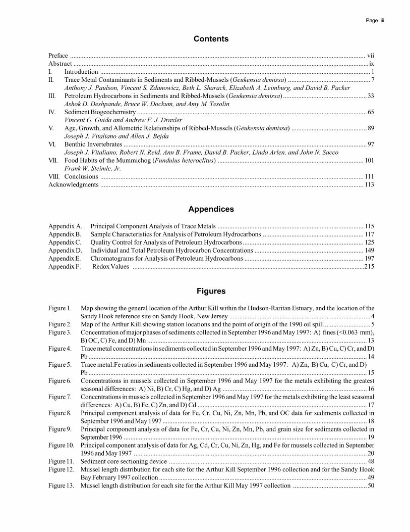
Contents

Preface ................................................................................................................................................................................ viiAbstract ................................................................................................................................................................................ i xI. Introduction ................................................................................................................................................................. 1II. Trace Metal Contaminants in Sediments and Ribbed-Mussels (Geukensia demissa) ................................................. 7

Anthony J. Paulson, Vincent S. Zdanowicz, Beth L. Sharack, Elizabeth A. Leimburg, and David B. PackerIII. Petroleum Hydrocarbons in Sediments and Ribbed-Mussels (Geukensia demissa) .................................................. 33

Ashok D. Deshpande, Bruce W. Dockum, and Amy M. TesolinIV. Sediment Biogeochemistry ......................................................................................................................................... 65

Vincent G. Guida and Andrew F. J. DraxlerV. Age, Growth, and Allometric Relationships of Ribbed-Mussels (Geukensia demissa) ............................................. 89

Joseph J. Vitaliano and Allen J. BejdaVI. Benthic Invertebrates ................................................................................................................................................. 97

Joseph J. Vitaliano, Robert N. Reid, Ann B. Frame, David B. Packer, Linda Arlen, and John N. SaccoVII. Food Habits of the Mummichog (Fundulus heteroclitus) ....................................................................................... 101

Frank W. Steimle, Jr.VIII. Conclusions ............................................................................................................................................................. 111Acknowledgments ............................................................................................................................................................. 113

Appendices

Appendix A. Principal Component Analysis of Trace Metals ....................................................................................... 115Appendix B. Sample Characteristics for Analysis of Petroleum Hydrocarbons ............................................................ 117Appendix C. Quality Control for Analysis of Petroleum Hydrocarbons ........................................................................ 125Appendix D. Individual and Total Petroleum Hydrocarbon Concentrations ................................................................. 149Appendix E. Chromatograms for Analysis of Petroleum Hydrocarbons ....................................................................... 197Appendix F. Redox Values .............................................................................................................................................215

Figures

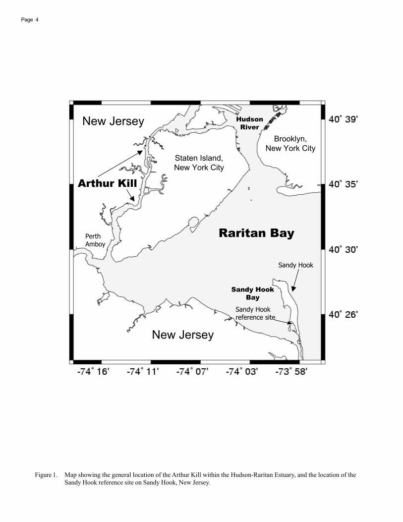
Figure 1. Map showing the general location of the Arthur Kill within the Hudson-Raritan Estuary, and the location of theSandy Hook reference site on Sandy Hook, New Jersey .................................................................................... 4

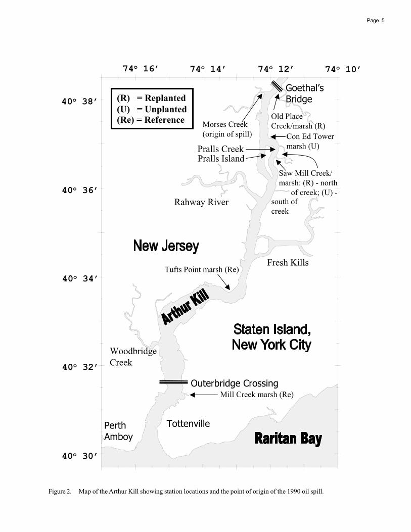
Figure 2. Map of the Arthur Kill showing station locations and the point of origin of the 1990 oil spill ........................... 5Figure 3. Concentration of major phases of sediments collected in September 1996 and May 1997: A) fines (<0.063 mm),

B) OC, C) Fe, and D) Mn ................................................................................................................................... 13Figure 4. Trace metal concentrations in sediments collected in September 1996 and May 1997: A) Zn, B) Cu, C) Cr, and D)

Pb ...................................................................................................................................................................... 14Figure 5. Trace metal:Fe ratios in sediments collected in September 1996 and May 1997: A) Zn, B) Cu, C) Cr, and D)

Pb ...................................................................................................................................................................... 15Figure 6. Concentrations in mussels collected in September 1996 and May 1997 for the metals exhibiting the greatest

seasonal differences: A) Ni, B) Cr, C) Hg, and D) Ag ...................................................................................... 16Figure 7. Concentrations in mussels collected in September 1996 and May 1997 for the metals exhibiting the least seasonal

differences: A) Cu, B) Fe, C) Zn, and D) Cd ..................................................................................................... 17Figure 8. Principal component analysis of data for Fe, Cr, Cu, Ni, Zn, Mn, Pb, and OC data for sediments collected in

September 1996 and May 1997 .......................................................................................................................... 18Figure 9. Principal component analysis of data for Fe, Cr, Cu, Ni, Zn, Mn, Pb, and grain size for sediments collected in

September 1996 ................................................................................................................................................. 19Figure 10. Principal component analysis of data for Ag, Cd, Cr, Cu, Ni, Zn, Hg, and Fe for mussels collected in September

1996 and May 1997 ........................................................................................................................................... 20Figure 11. Sediment core sectioning device ...................................................................................................................... 48Figure 12. Mussel length distribution for each site for the Arthur Kill September 1996 collection and for the Sandy Hook

Bay February 1997 collection ............................................................................................................................ 49Figure 13. Mussel length distribution for each site for the Arthur Kill May 1997 collection ............................................ 50

Page iv

Figure 14. Full GC-FID calibration chromatogram of all individual hydrocarbons and internal standards ........................ 51Figure 15. Chromatogram of a solution of the Restek diesel fuel oil #2 standard in methylene chloride with internal

standards added ............................................................................................................................................... 52Figure 16. Chromatograms of Sandy Hook ribbed-mussel homogenate spiked with 1000 μg of Restek diesel fuel oil #2

standard ............................................................................................................................................................ 53Figure 17. TPH concentrations for Old Place Creek and Mill Creek sediment samples ..................................................... 54Figure 18. TPH concentrations for Con Ed Tower sediment samples ................................................................................ 55Figure 19. Average TPH concentrations in surface sediments by site .............................................................................. 56Figure 20. Average TPH concentrations in ribbed-mussels by site .................................................................................. 57Figure 21. Box plot of the TPH concentrations in surface sediments ................................................................................ 58Figure 22. Correlation between TPH concentrations and TOC concentrations in Arthur Kill surface sediments from Old

Place Creek, Con Ed Tower, and Mill Creek marshes ........................................................................................ 59Figure 23. Correlation between TPH concentrations, mussel length, and percent lipid for Tufts Point ribbed-mussels ......... 60Figure 24. Correlation between TPH concentrations and percent lipid in Saw Mill Creek North ribbed-mussels, correlation

between mussel length and percent lipid in Saw Mill Creek South ribbed-mussels, and correlation betweenmussel length and percent lipid in Mill Creek ribbed-mussels .......................................................................... 61

Figure 25. Diagramatic view of DIW equilibration device in soil ....................................................................................... 76Figure 26. Depth profiles of redox potential for stations at replanted marsh sites in fall 1996 and spring 1997, including

duplicate profiles for each station .................................................................................................................... 77Figure 27. Depth profiles of redox potential for stations at reference marsh sites in fall 1996 and spring 1997, including

duplicate profiles for each station .................................................................................................................... 78Figure 28. Depth profiles of redox potential for stations at unplanted marsh sites in fall 1996 and spring 1997, including

duplicate profiles for each station .................................................................................................................... 79Figure 29. Seasonal patterns in interstitial soluble sulfide from replanted marsh stations ................................................ 80Figure 30. Seasonal patterns in interstitial soluble sulfide from unplanted marsh stations ............................................... 81Figure 31. Seasonal patterns in interstitial soluble sulfide from reference marsh stations ................................................ 82Figure 32. Seasonal values of TOC in surface sediments arranged by station, site, and replanting treatment ................. 83Figure 33. Mean LC in surface sediments taken from two stations per site in May 1998 .................................................. 84Figure 34. Log10 soluble sulfide plotted against mean redox potential for all nonzero sulfide values grouped by marsh

replanting status ............................................................................................................................................... 85Figure 35. Relationship between sediment surface TOC and silt/clay content ................................................................. 86Figure 36. Age-frequency distribution of ribbed-mussels collected at Old Place Creek and Saw Mill Creek North, Saw Mill

Creek South and Con Ed Tower, and Tufts Point and Mill Creek in September 1996 ....................................... 92Figure 37. Length-frequency distribution of ribbed-mussels collected at Old Place Creek and Saw Mill Creek North, Saw

Mill Creek South and Con Ed Tower, and Tufts Point and Mill Creek in September 1996 ................................ 93Figure 38. Growth of 2-, 3-, and 4-yr-old ribbed-mussels collected at the six Arthur Kill sites during September 1996 ........... 94

Tables

Table 1. Trace metal quality assurance data ................................................................................................................... 21Table 2. Metal concentrations in sediments in September 1996 ..................................................................................... 22Table 3. Metal concentrations in sediments in May 1997 .............................................................................................. 24Table 4. Trace metal statistics for sediments from the Arthur Kill and other areas in the region ................................... 26Table 5. Metal concentrations in ribbed-mussels in September 1996 ............................................................................. 27Table 6. Metal concentrations in ribbed-mussels in May 1997 ...................................................................................... 29Table 7. Trace metal statistics for ribbed-mussels from the Arthur Kill and other areas in the region ........................... 31Table 8. Correlations between metals and sediment characteristics, and among metals, in ribbed-mussels, where r

>0.80 ................................................................................................................................................................. 32Table 9. Concentrations of total petroleum hydrocarbons and of the total of the individual petroleum hydrocarbons for

surface sediments ............................................................................................................................................. 62Table 10. Concentrations of total petroleum hydrocarbons and of the total of the individual petroleum hydrocarbons for

sediment core sections ..................................................................................................................................... 63Table 11. Concentrations of total petroleum hydrocarbons and of the total of the individual petroleum hydrocarbons for

ribbed-mussels .................................................................................................................................................. 64

vPage

Table 12. Arthur Kill marsh biogeochemistry by treatment, site, station, and season ..................................................... 87Table 13. Average shell dimensions, shell dry weight, meat dry weight, and shell shape and body size relationships for

2-, 3-, and 4-yr-old ribbed-mussels collected at the six Arthur Kill sites during September 1996 ...................... 95Table 14. Invertebrate taxa collected at the six study sites in the Arthur Kill .................................................................. 99Table 15. Means/7-cm2 core for the abundances of all benthic invertebrates, oligochaetes, nematodes, and Manayunkia

aestuarina at each of the six study sites and two sampling dates in the Arthur Kill ..................................... 100Table 16. Percent frequency of occurrence of items or prey in mummichog stomachs from the six Arthur Kill sites during

September 1996 ............................................................................................................................................... 106Table 17. Mean percent stomach volume estimates of items or prey in mummichog stomachs from the six Arthur Kill sites

during September 1996 .................................................................................................................................... 107Table 18. Percent frequency of occurrence of items or prey in mummichog stomachs from the six Arthur Kill sites during

May-August 1997 ........................................................................................................................................... 108Table 19. Mean percent stomach volume estimates of items or prey in mummichog stomachs from the six Arthur Kill sites

during May-August 1997 ............................................................................................................................... 109

Acronyms

AAS = atomic absorption spectrophotometryANOVA = analysis of varianceBOD = biological oxygen demandCPI = carbon preference indexDARP = (NOAA) Damage Assessment and Restoration ProgramDDI = double de-ionizedDIW = de-ionized waterFID = flame ionization detection (detector)GC = gas chromatography (chromatogram)GC-FID = gas chromatography - flame ionization detectionGC/MS = gas chromatography/mass spectrometryHDPE = high-density polyethyleneHP = Hewlett-PackardLC = labile carbonMDL = method detection limitMS = mass spectrometrynd = not detectedNIST = (U.S. Department of Commerce) National Institute of Standards and TechnologyNJDEP = New Jersey Department of Environmental ProtectionNMFS = (U.S. Department of Commerce, NOAA) National Marine Fisheries ServiceNRC = National Research CouncilNYCDEP = New York City Department of Environmental ProtectionOC = organic carbonPAH = polycyclic aromatic hydrocarbonPCA = principal component analysisPD = percent differenceQA = quality assuranceRPD = relative percentage differenceRSD = relative standard deviationSMRT = (New York City Department of Parks and Recreation) Salt Marsh Restoration TeamSRM = standard reference materialTIPH = total of individual petroleum hydrocarbonsTOC = total organic carbonTPH = total petroleum hydrocarbonsWI = weathering index

Page vi

viiPage

PREFACE

For further information on the oil spill in the Arthur Kill, as well as pictures of the marsh sites and plantings, see theNational Oceanic and Atmospheric Administration (NOAA), Damage Assessment and Restoration Program (DARP), ExxonBayway Wetland Acquisition and Restoration webpage (http://www.darp.noaa.gov/neregion/exbw.htm). DARP is a col-laborative effort among NOAA’s National Ocean Service, National Marine Fisheries Service, and the Office of GeneralCounsel. DARP’s mission is to restore coastal and marine resources that have been injured by releases of oil or hazardoussubstances and to obtain compensation for the public’s lost use and enjoyment of these resources.

Page viii

ixPage

ABSTRACT

On January 1 and 2, 1990, a 576,000-gal oil spill seriously damaged the salt marshes of the Arthur Kill, the straitseparating Staten Island, New York, from New Jersey. The New York City Salt Marsh Restoration Team (SMRT) implementeda multiyear restoration and monitoring project to restore those parts of the marshes directly impacted by the oil spill.Restoration activities included successfully reintroducing Arthur-Kill-propagated saltmarsh cordgrass, Spartina alterniflora,and monitoring several parameters both in oiled marshes that were replanted and in oiled marshes that were left for naturalrecovery. Those parameters included: peak standing biomass, stem and flower density, and height of S. alterniflora;sediment total petroleum hydrocarbons (TPH); density of ribbed-mussels (Geukensia demissa); fish abundance and diver-sity; and wading bird (i.e., egret) foraging success.

Results of the monitoring suggest that the replanting of S. alterniflora was very important for recovery and restorationof the saltmarsh ecosystem. This replanting of S. alterniflora provides much of the structural component of the marsh;restoring this component to levels found elsewhere in the Arthur Kill is important to the other members of the food web, suchas the mussels, mummichogs, and birds. It is particularly significant in an urbanized landscape, where habitats are few andisolated.

However, questions remain as to the ecological viability and functional equivalency of these marshes. The problem iscompounded because not only was almost every low marsh within the Arthur Kill affected to some extent by the 1990 spill,but this estuary is heavily urbanized and degraded; its marshes are continuously impacted by contaminants and otheranthropogenic influences. In 1996 and 1997, the National Marine Fisheries Service (NMFS) sought to supplement the SMRTmonitoring efforts via a preliminary characterization and assessment of marshes that were oiled and replanted, marshes thatwere oiled but not planted, and nearby pre-existing S. alterniflora reference marshes, with a view toward noting anydifferences among the marshes, especially those that might be attributable to the replanting efforts. The measured param-eters include trace metal and hydrocarbon contaminants in ribbed-mussels and sediments, sediment biogeochemistry, ageand growth of ribbed-mussels, macrobenthic distribution and abundance, and diets of the mummichog (Fundulus heteroclitus).Sampling occurred in fall 1996 and spring-summer 1997.

Results of the NMFS study are less clear than those of the previous SMRT monitoring effort with regard to the benefitsof replanting, or even to the differences among sites. Trace metal concentrations in the sediments at each marsh were sitespecific and more dependent upon the general characteristics of the sediment, such as the percentage of fine-grainedsediments and iron content, than upon whether or not the marsh was replanted. Compared to concentrations from a referencemarsh outside the Arthur Kill, metal concentrations in sediments from the entire Arthur Kill were elevated. There were noconsistent differences in metal concentrations in mussels collected from replanted and unplanted marshes, while concentra-tions of many metals in mussels from two of three reference marshes were significantly lower. However, as with the metalconcentrations in the sediments, replanting may not have had a great effect on the levels of trace metals in the mussels.

The TPH concentrations in surface sediments from the southernmost reference marsh were numerically the lowest,those from the northernmost oiled and replanted marsh were intermediate, and those from one oiled but unplanted barrenmarsh were the highest; residual oil is still evident in sediments at this latter marsh. The lower levels of oil at the reference andreplanted marshes may be due to oxidation and weathering of the oil, perhaps caused by the physical disturbance of plantingand by the mineralization of oil by microbes around the roots of S. alterniflora. The TPH concentrations in mussels from allmarshes were low, were not significantly different, and showed no temporal trend; thus, replanting efforts do not appear tohave affected the levels of TPH in the mussels.

For biogeochemistry, the spatio-temporal patterns of porewater redox potential, soluble sulfide, and total organiccarbon in the marsh sediments showed statistically significant differences with depth and season. However, these differ-ences were not meaningful for assessment of replanting success because they appeared to owe more to the peculiarities ofindividual sampling stations within each of the marshes than to replanting status. Quantitative differences among stationdata within each marsh were so large, and distributions of values at those stations were so skewed, as to render differencesuninterpretable in terms of replanting. No patterns characteristic of replanted, unplanted, or reference marshes were identi-fied, nor were characteristic differences among sites fitting these treatment categories evident. The biogeochemistry appearsto be mediated by factors not clearly related to replanting. The marshes were heterogeneous with respect to these factors,confounding efforts to identify replanting-specific effects. Among those confounding factors were differences in grain sizedistribution, surface and subsurface hydrology, macrobiotic activity, and anthropogenic influences.

Ribbed-mussels from the replanted sites were younger, smaller, weighed less, and grew slower than mussels from thesouthernmost Arthur Kill reference site. The older, larger mussels collected at the reference marsh represent cumulativegrowth processes over many generations at a mature and relatively undisturbed marsh that was minimally affected by the oilspill. The younger, smaller mussels collected at the replanted sites most likely reflect growth processes since replanting.Although the chronic effect of oil from the spill and the disturbance caused by the replanting process may have affectedgrowth rates at the replanted sites, other natural and anthropogenic site-specific factors may also have been responsible.

Page x

The invertebrate taxa found within the sediments of the Arthur Kill marshes appear to be similar to invertebrate taxafound in S. alterniflora marshes elsewhere. Abundances of most taxa were highest in the spring. Although there may besimilarities in invertebrate abundances between the replanted and reference marshes, quantitative evaluation was con-founded due to the low number of replanted and reference sites sampled and to the high variability in the data, which istypical of benthic surveys.

The high percentages of detritus and algae, as opposed to live prey, in the mummichog stomachs may indicate a poordiet in a polluted environment, as suggested by previous studies. The mummichog diets may or may not have been sitespecific. A more thorough investigation would be necessary to discern such patterns in the data, as has been demonstratedfor several of our other investigations.

In conclusion, although replanting of the oil-damaged Arthur Kill marshes by SMRT may have successfully “restored”them, at least structurally, to the level of the existing marshes found within the Arthur Kill, because this is an urban estuary,the extent to which the ecological functions of these marshes have been restored is more difficult to ascertain due toconfounding factors such as pollution and other anthropogenic impacts. Also, the time span of the NMFS studies may havebeen too short and the number of treatment sites chosen may have been too small to accurately assess the performance ofthe replanted marshes, especially given the many scales of natural spatial and temporal variability and anthropogenicperturbations inherent in this ecosystem. Nevertheless, SMRT continues to replant and monitor these marshes wherenecessary, insuring that this vital habitat is protected from further loss and degradation.

1Page

I. INTRODUCTION

wetland restoration projects exist even today,” althoughauthors such as Short et al. (2000) are in the process ofdeveloping success criteria for estuarine restorationprojects. In fact, the term “restored” itself is not quite cor-rect: most current research in this field focuses on createdor constructed salt marshes [marshes created in responseto mitigation efforts; e.g., Zedler et al. (1997)], rather thanthose that have been restored or rehabilitated as a resultof a severe environmental impact. Thus, although the re-planting of S. alterniflora in the Arthur Kill was consideredboth successful and exceptional, and some SMRT monitor-ing results showed increased aquatic faunal and avian abun-dances at replanted sites (C. Alderson et al., Salt MarshRestoration Team, Natural Resources Group, New York CityParks, 200 Nevada Ave., Staten Island, NY, pers. comm. andunpubl. data), questions remain as to the ecological viabil-ity and functional equivalency of these marshes.

The problem is compounded because not only was al-most every low marsh within the Arthur Kill affected tosome extent by the 1990 spill, but this estuary is also heavilyurbanized, and the marshes are continuously impacted byurban runoff, contaminants, floatables, bank erosion, andillegal dumping which together can severely restrict naturalrecolonization of S. alterniflora. Thus, it may be difficult todetect differences in the ecosystem functions between thereplanted marshes and the pre-existing marshes within theArthur Kill. Even if differences are detected, it may be im-possible to attribute these differences to the replanting ef-forts or to the oil from the spill after so many years. Thesedifficulties are often encountered when undertaking envi-ronmental impact or restoration studies, particularly in ur-ban wetland habitats (Ehrenfeld 2000). Thus, as a first step,Ehrenfeld (2000) states: “Measures of restoration successand functional performance [in urban wetlands] must startwith an appreciation and assessment of the particular con-ditions imposed by the urban environment. These condi-tions can be identified, measured, and incorporated intoassessment protocols for individual wetland functions.”

Therefore, the primary goal of this study is to supple-ment the SMRT monitoring efforts via a preliminary charac-terization and assessment of marshes that were oiled andreplanted, marshes that were oiled but not planted, andnearby pre-existing S. alterniflora reference marshes, witha view toward noting any differences among sites, espe-cially those that might be attributable to the replanting ef-forts. Measured parameters include trace metals and hy-drocarbon contaminants in ribbed-mussels and sediments,sediment biogeochemistry, age and growth of ribbed-mus-sels, macrobenthic distribution and abundance, and dietsof the common mummichog (Fundulus heteroclitus). Moni-toring by itself often centers only on the structural attributesof the wetland; explicit measures of function, such as bio-geochemistry and the trophic linkages between the fish andbenthic communities (e.g., Moy and Levin 1991) can pro-

On January 1 and 2, 1990, an oil spill of 576,000 gal ofNo. 2 heating oil from an underwater Exxon pipeline seri-ously affected wildlife and aquatic plant communities of theArthur Kill, the strait separating Staten Island, New York,from New Jersey (Burger 1994; Figures 1 and 2). The leakoccurred at Morses Creek in the northern reach of the Kill,and affected areas as far north as the Kill van Kull andNewark Bay, and as far south as the Outerbridge Crossing.The total petroleum hydrocarbon (TPH) content of sedi-ments in the area was as high as 120,000 μg/g, and exceeded1000 μg/g in about 50% of the sediments tested (LouisBerger and Associates 1991). In areas closest to the spill,the dominant vegetation of the low marsh -- saltmarshcordgrass (Spartina alterniflora) -- was eradicated, andmussel beds were heavily damaged, locally experiencing upto 100% mortality (Louis Berger and Associates 1991).Approximately 700 aquatic birds were killed outright, andthe 1990 breeding season was seriously disrupted.

The New York City Department of Parks and Recreation’sSalt Marsh Restoration Team (SMRT) implemented amultiyear restoration and monitoring project to restore thoseparts of the marshes directly impacted by the 1990 oil spill.Restoration activities included the successful reintroduc-tion of over 9 acres of Arthur Kill-propagated S. alterniflora(Bergen et al. 2000). The SMRT has been monitoring sev-eral parameters both in oiled marshes that were replantedand in oiled marshes that were left for natural recovery.Those parameters included: peak standing biomass, stemand flower density, and height of saltmarsh cordgrass; sedi-ment TPH; density of ribbed-mussels (Geukensia demissa);fish abundance and diversity; and wading bird (egret) for-aging success (Bergen et al. 2000; C. Alderson et al., SaltMarsh Restoration Team, Natural Resources Group, NewYork City Parks, 200 Nevada Ave., Staten Island, NY, pers.comm. and unpubl. data).

Understanding the development and functional valueof restored salt marshes requires an understanding of hownatural salt marshes function. There have been severalstudies comparing the relative and functional value of re-stored marshes to natural marshes (e.g., Cammen 1976; Raceand Christie 1982; Pacific Estuarine Research Laboratory1990; LaSalle et al. 1991; Minello and Zimmerman 1992;Zedler 1993; Matthews and Minello 1994; Sacco et al. 1994;Havens et al. 1995; Thompson et al. 1995; Levin et al. 1996;Simenstad and Thom 1996; see also Kentula 2000). How-ever, many restored wetlands have not been scientificallyevaluated for their success in approaching the equivalentfunctional levels of natural wetland habitats; indeed, deter-mining the “functional equivalency” of a restored wetlandcompared to a natural wetland is very difficult, and apprais-ing the success of a restoration is problematic (e.g., seeSimenstad and Thom 1996; Kentula 2000; Zedler andCallaway 2000). Lewis (2000) noted that “no generally ac-cepted and applied criteria for establishing goals for coastal

Page 2

vide a more integrated assessment of ecosystem processes,as well as measure the progress of restoration (Simenstadand Thom 1996). Thus, this preliminary characterization,although limited, both complements and goes beyond thecurrent monitoring studies of New York’s SMRT, and mayallow us to better evaluate our ability to restore the func-tional attributes of this habitat, as well as to identify poten-tial indicators of habitat and living marine resource health,impacts, and recovery within a heavily urbanized and de-graded estuary.

SITE DESCRIPTIONS

Six Arthur Kill marshes were selected: two oiled andreplanted, two oiled but unplanted, and two pre-existing S.alterniflora reference marsh sites (Figures 1 and 2). For thetrace metals and hydrocarbon analysis studies, mussels werecollected farther south and east in the relatively pristineSandy Hook Bay (Figure 1) to use as an additional refer-ence.

Sampling occurred in September 1996 and May 1997.Mummichogs were scarce in spring 1997, so that year, sam-pling for those fish occurred from May until early August.

Replanted and Unplanted Sites

Old Place Creek and marsh surrounds the Goethal’sBridge in the northern end of the Arthur Kill betweenElizabethport Reach and Gulfport Reach. The site is almostdirectly across from the origin of the spill and was heavilyoiled, with replanting occurring around 1993. Oily residueswere still found at this site in 1996-97. The shoreline washeavily impacted by tugboat and wind-generated waves.The combination of wave energy and Old Place Creek’sclose proximity to the Bayway Refinery have left parts ofthe shoreline devoid of both vegetation and the thick lay-ers of peat generated since the last glaciation. Some partsof the marsh (outside of our study area) were fouled by anasphalt spill in the 1980s, and the substrate was laterstripped. For a further description of this marsh, the impactof the oil spill, and subsequent replanting, see Bergen et al.(2000), as well as Blanchard et al. (2001).

The Consolidated Edison Tower (i.e., “Con Ed Tower”)site is located at the junction of the northern end of Prall’sCreek and the Arthur Kill. The area was not replanted (al-though it may be in the near future) and was barren; thesubstrate consisted of a combination of asphalt-coveredpeat, exposed peat, and sand-and-gravel-covered peat orasphalt. The substrate still had oily residues at the time ofour sampling.

The Saw Mill Creek North marsh site is located on thenorthern shoreline of Saw Mill Creek. The replanted siteoccupied a narrow 3-6 m wide band which ran 91 m in lengthfrom the mouth of the creek east into the full marsh. Dam-age and destruction by oil at this site consisted of the loss

of S. alterniflora and subsequent erosion of peat and adja-cent high marsh. Replanting occurred in 1992.

The unplanted Saw Mill Creek South site is on the op-posite (south) shore of the creek. The width of the de-nuded area was not as wide as that on the north shore.Since the oil spill, erosion of the denuded south banks hasoccurred, but S. alterniflora has re-established itself with-out the need for replanting. Unlike the barren Con Ed Towersite, the unplanted Saw Mill Creek South site was visuallyindistinguishable from the replanted Saw Mill Creek Northsite by 1996.

Reference Sites

Many authors have noted the importance of choosingreference sites that adequately reflect the conditions of therestoration site, and that encompass the known variation ofthe group of wetlands in the study (e.g., Brinson andRheinhardt 1996; Kentula 2000; Short et al. 2000). Refer-ence sites in urban areas will, and should, reflect the reali-ties of the urban context [see Ehrenfeld (2000) and authorscited therein for an extended discussion of reference sitesin urban wetland restoration studies]. Thus, at least one ofthe two pre-existing S. alterniflora reference marshes wechose was affected to some degree by the oil spill, and bothare continually affected by anthropogenic impacts, as areall marshes within the Arthur Kill itself. In fact, it would nothave been possible or even feasible to find or use a “pris-tine” marsh within the Arthur Kill.

The first site, Tufts Point, is located midway on theNew Jersey side, and extends out into the Kill where it turnssharply to the west between Fresh Kills Reach and PortReading Reach. After the oil spill, the site suffered some“medium oiling” according to Louis Berger and Associates(1991). There was a high mortality of the ribbed-mussel, acommon bivalve mollusk residing in the low marsh and pre-dominantly attached to the stems and roots of S.alterniflora. Nevertheless, relative to the more northernmarshes, the site did not suffer extensive damage after the1990 spill, and was considered by SMRT to be in goodcondition. Therefore, we considered it as a reference marsh.

The second reference site, Mill Creek marsh, is locatedin the Outerbridge Reach, just to the south of the OuterbridgeCrossing on Staten Island. It was our southernmost site.The study marsh itself was located on an island right at themouth of the creek; at very low tides the water over thesurrounding mudflats was shallow enough to allow easyaccess to the mainland. Although Mill Creek marsh waslocated in the “lightly-impacted” zone (Louis Berger andAssociates 1991) of the 1990 spill, Louis Berger and Asso-ciates (1991) nevertheless observed no oiling there, anddeclared it a control site.

The Sandy Hook reference site used for contaminantanalyses was located on the western shoreline of the bar-rier beach peninsula, in Sandy Hook Bay (Figure 1), wherethere are a series of marshes and mud flats that are exposed

3Page

during periods of low tide in an area south of SpermacetiCove and north of Plum Island. The site was considered tobe relatively clean, especially compared to the Arthur Kill.

REFERENCES CITED

Bergen, A.; Alderson, C.; Bergfors, R.; Aquila, C.; Matsil,M.A. 2000. Restoration of a Spartina alterniflora saltmarsh following a fuel oil spill, New York City, NY. Wet-lands Ecol. Manage. 8:185-195.

Blanchard, P.P., III; Kerlinger, P.; Stein. M.J. 2001. Anislanded nature -- natural area conservation in westernStaten Island, including the Harbor Herons Region.Washington, DC: The Trust for Public Land, and, NewYork City Audubon Society; 224 p.

Brinson, M.M.; Rheinhardt, R. 1996. The role of referencewetlands in functional assessment and mitigation. Ecol.Appl. 6:69-77.

Burger, J., editor. 1994. Before and after an oil spill: theArthur Kill. New Brunswick, NJ: Rutgers Univ. Press;305 p.

Cammen, L.M. 1976. Abundance and production ofmacroinvertebrates from natural and artificially estab-lished salt marshes in North Carolina. Am. Midl. Nat.96:487-493.

Ehrenfeld, J.G. 2000. Evaluating wetlands within an urbancontext. Ecol. Eng. 15:253-265.

Havens, K.J.; Varnell, L.M.; Bradshaw, J.G. 1995. An as-sessment of ecological conditions in a constructed tidalmarsh and two natural reference tidal marshes in coastalVirginia. Ecol. Eng. 4:117-141.

Kentula, M.E. 2000. Perspectives on setting success crite-ria for wetland restoration. Ecol. Eng. 15:199-209.

LaSalle, M.W.; Landin, M.C.; Sims, J.G. 1991. Evaluation ofthe flora and fauna of a Spartina alterniflora marshestablished on dredged material in Winyah Bay, SouthCarolina. Wetlands 11:191-208.

Levin, L.; Tally, D.; Thayer, G. 1996. Succession ofmacrobenthos in a created salt marsh. Mar. Ecol. Prog.Ser. 141:67-82.

Lewis, R.R., III. 2000. Ecologically based goal setting inmangrove forest and tidal marsh restoration. Ecol. Eng.15:191-198.

Louis Berger and Associates, Inc. 1991. Arthur Kill oildischarge study. Vol 1. Final report, and, Vol. 2. Appen-dices. Submitted to: New Jersey Department of Envi-ronmental Protection and Energy, Trenton, NJ.

Matthews, G.A.; Minello, T.J. 1994. Technology and suc-cess in restoration, creation, and enhancement ofSpartina alterniflora marshes in the United States. Vol.1 -- Executive summary and annotated bibliography.NOAA Coast. Ocean Prog. Decision Anal. Ser. 2.

Minello, T.J.; Zimmerman, R.J. 1992. Utilization of naturaland transplanted Texas salt marshes by fish and deca-pod crustaceans. Mar. Ecol. Prog. Ser. 90:273-285.

Moy, L.D.; Levin, L.A. 1991. Are Spartina marshes a re-placeable resource? A functional approach to evalua-tion of marsh creation efforts. Estuaries 14:1-16.

Pacific Estuarine Research Laboratory. 1990. A manual forassessing restored and natural coastal wetlands withexamples from southern California. Calif. Sea GrantRep. T-CSGCP-021.

Race, M.S.; Christie, D.R. 1982. Coastal zone development:mitigation, marsh creation, and decision-making.Environ. Manag. 6:317-328.

Simenstad, C.A.; Thom, R.M. 1996. Functional equiva-lency trajectories of the restored Gog-Le-Hi-Te estua-rine wetland. Ecol. Appl. 6:38-56.

Sacco, J.N.; Seneca, E.D.; Wentworth, T.R. 1994. Infaunalcommunity development of artificially established saltmarshes in North Carolina. Estuaries 17:489-500.

Short, F.T.; Burdick, D.M.; Short, C.A.; Davis, R.C.; Mor-gan, P.A. 2000. Developing success criteria for re-stored eelgrass, salt marsh and mud flat habitats. Ecol.Eng. 15:239-252.

Thompson, S.P.; Paerl, H.W.; Go, M.C. 1995. Seasonal pat-terns of nitrification and denitrification in a natural anda restored salt marsh. Estuaries 18:399-408.

Zedler, J.B. 1993. Canopy architecture of natural and plantedcordgrass marshes: selecting habitat evaluation crite-ria. Ecol. Appl. 3:123-138.

Zedler, J.B.; Callaway, J.C. 2000. Evaluating the progress ofengineered tidal wetlands. Ecol. Eng. 15:211-225.

Zedler, J.B.; Williams, G.D.; Desmond, J.S. 1997. Wetlandmitigation: can fishes distinguish between natural andconstructed wetlands? Fisheries 22:26-28.

PerthAmboy

Sandy Hook

Sandy Hookreference site

Staten Island,New York City

Brooklyn,New York City

New Jersey

New Jersey

Raritan Bay

Arthur Kill

HudsonRiver

Sandy HookBay

Page 4

Figure 1. Map showing the general location of the Arthur Kill within the Hudson-Raritan Estuary, and the location of theSandy Hook reference site on Sandy Hook, New Jersey.

74o 16’ 74o 12’ 74o 10’74o 14’

40o 38’

40o 32’

40o 30’

40o 34’

40o 36’

Goethal’sBridge

Morses Creek (origin of spill)

Old PlaceCreek/marsh (R)

Con Ed Towermarsh (U)Pralls Creek

Fresh Kills

Rahway River

WoodbridgeCreek

Mill Creek marsh (Re)Outerbridge Crossing

PerthAmboy

Tottenville

(R) = Replanted(U) = Unplanted(Re) = Reference

Tufts Point marsh (Re)

Pralls IslandSaw Mill Creek/marsh: (R) - north

of creek; (U) -south ofcreek

5Page

Figure 2. Map of the Arthur Kill showing station locations and the point of origin of the 1990 oil spill.

Page 6

7Page

II. TRACE METAL CONTAMINANTSIN SEDIMENTS AND RIBBED-MUSSELS (Geukensia demissa)

Anthony J. Paulson1, 2, 4, Vincent S. Zdanowicz3, 5, Beth L. Sharack1, 6,Elizabeth A. Leimburg1, 7, and David B. Packer1, 8

Postal Addresses: 1National Marine Fisheries Serv., 74 Magruder Rd., Highlands, NJ 07732; 3U.S. Customs Serv., 7501 Boston Blvd., Ste. 113, Springfield, VA 22153Current Address: 2U.S. Geological Survey, 1201 Pacific Ave., Ste. 600, Tacoma, WA 98402E-Mail Addresses: 4apaulson@usgs.gov; 5Vincent.Zdanowicz@customs.treas.gov; 6Beth.Sharack@noaa.gov; 7Elizabeth.Leimburg@noaa.gov; 8Dave.Packer@noaa.gov

INTRODUCTION

Bioaccumulation of metals in mussels depends not onlyon metal concentrations in the sediments (Hummel et al.1997), but also the physiological state of the organism (e.g.,season and environmental factors) and the biogeochemis-try of the sediments (e.g., iron (Fe) content, organic carbon(OC) content, and oxidation-reduction condition). Tracemetals were analyzed in mussels and sediments in the ArthurKill to determine if the biogeochemical processes that con-trol bioaccumulation were affected by replanting of S.alterniflora at the previously oiled sites. Since the replantedsites were not sampled before replanting, pairs of unplanted,replanted, and reference sites in the Arthur Kill were sampledfor mussels and sediments in September 1996 and May 1997.Sampling at the unplanted sites (i.e., Con Ed Tower and SawMill Creek South sites) occurred 6 yr after the 1990 ExxonBayway oil spill. At the time of initial sampling, S. alternifloraplanted in 1992 had been growing at the Saw Mill CreekNorth site for 4 yr, while the S. alterniflora planted at theOld Place Creek site in 1993 had been growing for 3 yr. TwoArthur Kill reference sites (i.e., Tufts Point and Mill Creek)and a regional reference site (i.e., Sandy Hook) were alsosampled.

This chapter only addresses: 1) the level of contamina-tion of Arthur Kill sediments and mussels, and 2) whetherreplanting is the dominant factor controlling metal concen-trations in sediment and mussels. More specific interac-tions between bioaccumulation in mussels and sedimentgeochemistry will not be addressed in this chapter.

METHODS AND MATERIALS

All implements and plastic containers used for collect-ing, transporting, processing, and storing sediment andmussel samples for metals analyses were decontaminatedby rinsing in dilute, ultrapure nitric acid, then doubly in de-ionized (DDI) water.

Sediments

For collecting sediment samples, four stations were se-lected along a transect at 0.2 m above the mid-tide level ateach of the six sites within the Arthur Kill. Locations withequal tidal height were chosen to minimize station-to-sta-tion differences in surface (tidal) hydrology. The positionsof the stations along the transect were chosen based on theneed to minimize disturbance to the site. Also, access tothe specific sites was affected by unique logistical difficul-ties. For this reason, distances between stations along thetransect at a site ranged from 2 to 20 m apart, and the totallength of the transects among sites ranged from 12 m at SawMill Creek South to 39.5 m at Old Place Creek. At the re-planted and reference marsh sites, stations along thetransect were located within the vegetated zone. At Con EdTower, the transect was in a wide unvegetated area, andstations were located in mud and peat that contained chunksof asphalt. At Saw Mill Creek South, the transect was alongthe edge of the cordgrass and barren mud and peat banks.

Sediment samples for grain size analysis were collectedat each of the four stations within each of the six sites inSeptember 1996 (one core per station) by using 28-mm-in-ternal-diameter, plastic-core tubes, and were frozen for trans-port back to the laboratory. The particle size distribution ofthe sediment mineral fraction was determined by modifyingthe standard wet and dry sieving procedures of Ingram(1971), Galehouse (1971), and Folk (1980). The particle up-per size limit chosen was > -2φ (i.e., pebble/granule bound-ary), and the particle lower size limit was >4φ (i.e., mud,composed of silt and clay). The top 5 cm of each frozencore were extracted, treated with several milliliters of 30%H2O2, and heated to digest any organic material. The samplesoften contained large sections of S. alterniflora rhizomesand stems, which were removed. Each sample was then wetsieved with a 63-μm sieve to separate the coarse sedimentfrom the mud. While the mud remained in distilled water,the coarse fraction was dried and mechanically sievedthrough different-sized sieves to separate out the various

Page 8

coarse size fractions, plus any remaining mud. After weigh-ing the dried coarse fractions, the mud from both wet anddry sieving procedures was combined, dried, and weighed.For samples from the Con Ed Tower site, deposits of tarprevented us from performing any grain size analysis.

For determination of total OC in the sediments, see Chap-ter IV, “Sediment Biogeochemistry.”

For trace metal analyses, sediment cores were collectedwith 31-mm-diameter acrylic tubes at the four representa-tive locations within each of the six Arthur Kill sites and attwo locations within the regional reference site (i.e., SandyHook). The top 1-cm section from each core was driedovernight at 60-65°C, the debris was removed, and the re-maining sample was pulverized. Ten milliliters of trace-metal-grade concentrated HCl was added to a 100-ml Pyrex beakercontaining 1-10 g of dried sediment, and was allowed toreact with the sediment for 15 min (Zdanowicz et al. 1995).After the addition 10 ml of concentrated HNO3, the sedi-ment slurry was then allowed to stand for 2 hr. The slurrywas then taken to dryness over low heat. After the additionof 25 ml of 0.1-M aqua regia, this slurry stood overnight atroom temperature. The volume of liquid was reduced toabout 10 ml over low heat, and the slurry was filtered throughacid-cleaned, #41 Whatman filter paper using additionalDDI to rinse the beaker. DDI was added to bring the filtrateto a final volume of 25 ml.

The resulting solutions were analyzed for iron (Fe),chromium (Cr), copper (Cu), nickel (Ni), zinc (Zn), manga-nese (Mn), and lead (Pb) by using flame atomic absorptionspectrophotometry (AAS). Six procedural blanks and fivereplicates of standard reference material (SRM) NIST 1645(river sediment) obtained from the National Institute of Stan-dards and Technology (NIST) were also analyzed by thesame procedure. Table 1 shows the quality assurance datafor the trace metals. Except for Ni and Pb in the May 1997Sandy Hook samples, metal values in the sediments wereabove detection limits (see Table 2). Recoveries for NIST1645 ranged between 90 and 98% . Within the Arthur Killsamples, outliers were identified using the Grubbs test (Sokaland Rohlf 1981), and were not used to calculate any statis-tical parameter. Differences in mean metal concentrationsamong groups of samples from different sites for each yearwere investigated using analysis of variance (ANOVA; P =0.05) and Duncan’s multiple range test.

Mussels

Ribbed-mussels were collected randomly at each site inSeptember 1996 and May 1997. Owing to the sparse den-sity of the mussels, to the limited time available for sam-pling (i.e., between high tides), and to the desire not todisturb the sites any more than necessary, the first 60-70specimens that were found were collected. At the Saw Mill

Creek South site, sampling was impeded by tall S.alterniflora, so it was possible to collect only 34 specimensin 1996.

After being transported to the NMFS James J. HowardMarine Sciences Laboratory in Sandy Hook, New Jersey, inplastic bags under ice, mussels from each site were sepa-rated by size into two roughly identical groups, one formetals analysis and one for hydrocarbon analysis. In orderto obtain specimens of comparable size at each site for metalanalysis, a length range between 55 and 67 mm was se-lected. This was the smallest size range that provided atleast five individuals per site. At sites where there weremore than five specimens within this range, samples wereselected using the following procedure. The size range wasdivided into five bins. One specimen per bin was selectedrandomly. If a bin contained no specimens, an alternate binwas selected at random, and a specimen was selected ran-domly from it. For the given length range, the average wetweight (15.65±2.70 g) of tissue collected in May 1997 fromthe Mill Creek site was significantly greater than the weightsof samples for the 13 other collections (13.32±2.10 g).

Mussel specimens for metal analysis were allowed todepurate overnight in ambient, laboratory supplied seawa-ter at 4°C. After removing extraneous material from the shell(mud, barnacles, etc.), total weight and length were recordedfor each specimen. The tissue (i.e., soft parts) was thenexcised, and stored in a vial at -20°C until analysis. Five orsix individual samples per site were analyzed for metals.After thawing, the entire soft tissue was placed in a Teflonvial and weighed. The tissue was dried overnight at 60-65°C and reweighed to obtain a dry weight. Five millilitersof ultrapure concentrated HNO3 was added to the samplewhich was typically 1 g. The vials were allowed to stand atroom temperature for 2-4 hr. Vials were then capped andplaced inside Teflon-lined bombs, and the tissue was di-gested overnight at 120°C. After cooling, bombs werevented, the vials were removed, and the digests were al-lowed to degas at room temperature overnight. The digestswere then quantitatively transferred to 25-ml glass gradu-ated cylinders and brought to volume using DDI water. Theresulting solutions were analyzed for Fe, Cu, and Zn byusing flame AAS, for Cr, Ni, silver (Ag),and cadmium (Cd)by using graphite furnace AAS, and for mercury (Hg) byusing cold-vapor AAS. Nine procedural blanks and ninereplicates of NIST 1566a (freeze-dried oyster tissue) werealso analyzed using the same procedure. Details of thesample digestion and analysis procedure can be found inZdanowicz et al. (1993).

Values for all specimens were above detection limits.Average SRM recoveries ranged from 96-102% (Table 1). Amajority of variables for two Con Ed Tower samples col-lected in May 1997 were found to be outliers, and all datafrom these two samples were disregarded (see Table 6).

9Page

RESULTS

Sediments

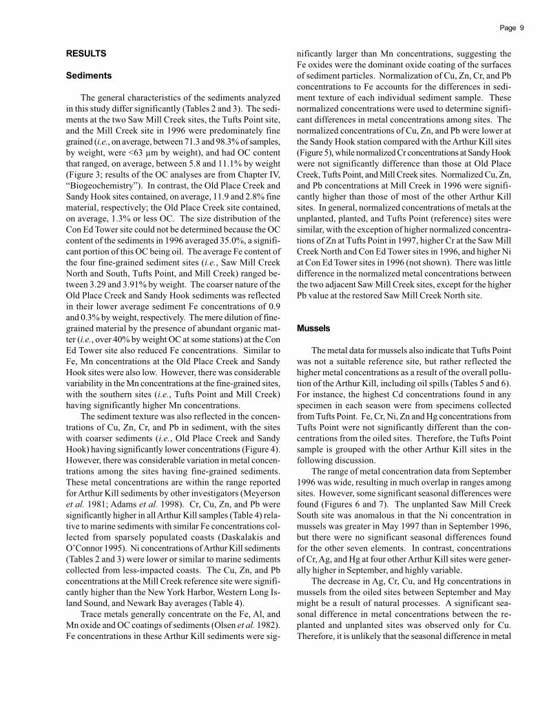
The general characteristics of the sediments analyzedin this study differ significantly (Tables 2 and 3). The sedi-ments at the two Saw Mill Creek sites, the Tufts Point site,and the Mill Creek site in 1996 were predominately finegrained (i.e., on average, between 71.3 and 98.3% of samples,by weight, were <63 μm by weight), and had OC contentthat ranged, on average, between 5.8 and 11.1% by weight(Figure 3; results of the OC analyses are from Chapter IV,“Biogeochemistry”). In contrast, the Old Place Creek andSandy Hook sites contained, on average, 11.9 and 2.8% finematerial, respectively; the Old Place Creek site contained,on average, 1.3% or less OC. The size distribution of theCon Ed Tower site could not be determined because the OCcontent of the sediments in 1996 averaged 35.0%, a signifi-cant portion of this OC being oil. The average Fe content ofthe four fine-grained sediment sites (i.e., Saw Mill CreekNorth and South, Tufts Point, and Mill Creek) ranged be-tween 3.29 and 3.91% by weight. The coarser nature of theOld Place Creek and Sandy Hook sediments was reflectedin their lower average sediment Fe concentrations of 0.9and 0.3% by weight, respectively. The mere dilution of fine-grained material by the presence of abundant organic mat-ter (i.e., over 40% by weight OC at some stations) at the ConEd Tower site also reduced Fe concentrations. Similar toFe, Mn concentrations at the Old Place Creek and SandyHook sites were also low. However, there was considerablevariability in the Mn concentrations at the fine-grained sites,with the southern sites (i.e., Tufts Point and Mill Creek)having significantly higher Mn concentrations.

The sediment texture was also reflected in the concen-trations of Cu, Zn, Cr, and Pb in sediment, with the siteswith coarser sediments (i.e., Old Place Creek and SandyHook) having significantly lower concentrations (Figure 4).However, there was considerable variation in metal concen-trations among the sites having fine-grained sediments.These metal concentrations are within the range reportedfor Arthur Kill sediments by other investigators (Meyersonet al. 1981; Adams et al. 1998). Cr, Cu, Zn, and Pb weresignificantly higher in all Arthur Kill samples (Table 4) rela-tive to marine sediments with similar Fe concentrations col-lected from sparsely populated coasts (Daskalakis andO’Connor 1995). Ni concentrations of Arthur Kill sediments(Tables 2 and 3) were lower or similar to marine sedimentscollected from less-impacted coasts. The Cu, Zn, and Pbconcentrations at the Mill Creek reference site were signifi-cantly higher than the New York Harbor, Western Long Is-land Sound, and Newark Bay averages (Table 4).

Trace metals generally concentrate on the Fe, Al, andMn oxide and OC coatings of sediments (Olsen et al. 1982).Fe concentrations in these Arthur Kill sediments were sig-

nificantly larger than Mn concentrations, suggesting theFe oxides were the dominant oxide coating of the surfacesof sediment particles. Normalization of Cu, Zn, Cr, and Pbconcentrations to Fe accounts for the differences in sedi-ment texture of each individual sediment sample. Thesenormalized concentrations were used to determine signifi-cant differences in metal concentrations among sites. Thenormalized concentrations of Cu, Zn, and Pb were lower atthe Sandy Hook station compared with the Arthur Kill sites(Figure 5), while normalized Cr concentrations at Sandy Hookwere not significantly difference than those at Old PlaceCreek, Tufts Point, and Mill Creek sites. Normalized Cu, Zn,and Pb concentrations at Mill Creek in 1996 were signifi-cantly higher than those of most of the other Arthur Killsites. In general, normalized concentrations of metals at theunplanted, planted, and Tufts Point (reference) sites weresimilar, with the exception of higher normalized concentra-tions of Zn at Tufts Point in 1997, higher Cr at the Saw MillCreek North and Con Ed Tower sites in 1996, and higher Niat Con Ed Tower sites in 1996 (not shown). There was littledifference in the normalized metal concentrations betweenthe two adjacent Saw Mill Creek sites, except for the higherPb value at the restored Saw Mill Creek North site.

Mussels

The metal data for mussels also indicate that Tufts Pointwas not a suitable reference site, but rather reflected thehigher metal concentrations as a result of the overall pollu-tion of the Arthur Kill, including oil spills (Tables 5 and 6).For instance, the highest Cd concentrations found in anyspecimen in each season were from specimens collectedfrom Tufts Point. Fe, Cr, Ni, Zn and Hg concentrations fromTufts Point were not significantly different than the con-centrations from the oiled sites. Therefore, the Tufts Pointsample is grouped with the other Arthur Kill sites in thefollowing discussion.

The range of metal concentration data from September1996 was wide, resulting in much overlap in ranges amongsites. However, some significant seasonal differences werefound (Figures 6 and 7). The unplanted Saw Mill CreekSouth site was anomalous in that the Ni concentration inmussels was greater in May 1997 than in September 1996,but there were no significant seasonal differences foundfor the other seven elements. In contrast, concentrationsof Cr, Ag, and Hg at four other Arthur Kill sites were gener-ally higher in September, and highly variable.

The decrease in Ag, Cr, Cu, and Hg concentrations inmussels from the oiled sites between September and Maymight be a result of natural processes. A significant sea-sonal difference in metal concentrations between the re-planted and unplanted sites was observed only for Cu.Therefore, it is unlikely that the seasonal difference in metal

Page 10

concentrations in mussels was influenced by the replant-ing effort.

Only the May data were used to determine geographi-cal differences in metal concentrations in mussels, sincethe September data were so highly variable. Relative to theoiled sites, Cr, Cu, and Hg concentrations in mussels weresignificantly lower at the Mill Creek and Sandy Hook sites,while Fe and Cu were significantly lower only at the SandyHook site. The range of concentrations of Ag, Ni, and Zn inmussels at both these reference sites significantly over-lapped the concentrations of some of the oiled sites.

For all elements in mussels, there were no clear differ-ences between the replanted and unplanted sites. Themussels from the unplanted Saw Mill Creek South site con-tained the highest concentrations of Fe, Cr, Cu, Ni, Ag, andHg. The close proximity and similar sediment characteris-tics (i.e., % fines and OC content) of the unplanted Saw MillCreek South and the replanted Saw Mill Creek North sitesprovide a valid comparison to test the effects of replanting.The concentrations of Ag and Cd were significantly higher(P <0.05) at the unplanted Saw Mill Creek South site, whilethe concentrations of Zn were significantly higher at theSaw Mill Creek North site. No significant differences werefound for Cr, Cu, Ni, Hg, and Fe.

Although mussels have been used extensively in ma-rine monitoring programs, these programs primarily use theblue mussel, Mytilus edulis. In one of the few studies inwhich the accumulation of metals was compared in differ-ent species of mussels, Nelson et al. (1995) state, “thesefindings highlight the fact that metal uptake in bivalves is acomplicated process that can be affected by many exog-enous and endogenous factors.” In keeping with their cau-tion, our ribbed-mussel data were compared only with otherribbed-mussel data (Table 7). Cr, Cu, and Zn concentra-tions in ribbed-mussels from Sandy Hook are comparablewith those from a clean site in East Sandwich, MA (Nelsonet al. 1995). In contrast, the metal concentrations in ribbed-mussels from the Arthur Kill are similar to those from thepolluted New Bedford Harbor, Massachusetts, and InnerMystic River Estuary, Connecticut (Nelson et al. 1995; Miller1988).

DISCUSSION

Sediments

Correlations among metal concentrations, grain size, andOC content were determined by two separate analyses be-cause of incomplete data. No correlations, though, couldbe calculated for the Sandy Hook site because of lack ofsufficient grain size data and lack of any OC data. In thefirst analysis, correlations were determined for the metaland OC data from each site for both 1996 and 1997 samplingperiods. In the second analysis, correlations were deter-mined for the metal and grain size data from each site exceptthe Con Ed Tower site for just the 1996 sampling period.

For the Old Place Creek site, the significant variabilityin both metal and OC concentrations among individual sedi-ment samples appears to be related to the portion of fine-grained sediments found in each sample. The 1996 metaldata from Old Place Creek, excluding Mn and Cu, were cor-related with the percentage of fine-grained sediment foundin each sample. When the entire Old Place Creek data set issubjected to correlation analysis using OC data (Table 8),the entire correlation matrix table is significant (r>0.80). Forthe fine-grained-sediment sites (i.e., Saw Mill Creek Northand South, Mill Creek, and Tufts Point), no significant cor-relations were found between Fe vs. Cr, Ni, Cu, Zn, or Pb.This lack of correlation is not surprising since Fe concen-trations within a site varied only over a very small range(Figure 3). For these fine-grained sediments, correlationsamong trace metals are not controlled by the concentra-tions of Fe oxides, but are controlled by how the trace met-als interact with the Fe oxide coating or by phases otherthan Fe oxides.

Different subsets of trace metals were highly correlatedfor the data sets from different sites. For instance, signifi-cant correlations were found among Pb, Cr, and Cu at theSaw Mill Creek North site (Table 8). It is interesting to notethat these three metals were negatively correlated with thepercentage of fine-grained sediments. This negative corre-lation suggests that Pb, Cr, and Cu are associated with acoarser type of particle. Significant correlations were alsofound among Cr, Ni, and Zn at the Con Ed Tower site, andamong Cr, Cu, Ni, and Pb at the Saw Mill South site.

The entire metals data set was subjected to principalcomponents analysis (PCA) using both the OC and grainsize data (see eigenvectors in Appendix Tables A1 and A2).When OC data are used, both sampling periods could beanalyzed, but without the Sandy Hook site. The Old PlaceCreek site is distinguished because of its lower metal con-centration (Figure 8). Except for one sample, the Mill Creeksite is separated from the other fine-grained stations in theArthur Kill. Although the 1996 Con Ed Tower site is sepa-rated from the rest of the sites with finer sediment, there isno distinct difference in replanted and unplanted sites.When only the 1996 metal data set was used with percent-age of fine-grained sediment data (Figure 9), the Sandy Hookand Old Place Creek sites again are differentiated from thefine-grained sediment sites. Among the fine-grained sedi-ment sites, only Mill Creek is distinguished.

Mussels

Trace metal concentrations in mussels were higher andmore highly variable in September 1996 than in May 1997.Of the eight metals analyzed, four (i.e., Cr, Ni, Cd, and Hg)were significantly lower in mussels at both reference sitesrelative to the other Arthur Kill sites, and two others (i.e., Feand Cu) were significantly lower only at the Sandy Hookreference site. Five metals showed higher concentrationsin mussels at the unplanted Saw Mill Creek South site com-

11Page

pared to the nearby replanted Saw Mill Creek North site.The lack of strong and consistent trends required higher-level statistical analysis of the data in order to draw anyconclusions concerning the effects of replanting. Correla-tions among metal concentrations in mussels were exam-ined for each station to determine if biogeochemical pro-cesses were causing similar trends for a subset of the met-als studied. In addition, the entire mussel data set wassubjected to PCA to determine if the data were separable bytype (i.e., unplanted, planted, or reference).

A few significant correlations between the concentra-tion of pairs of metals in mussels within a site were found atthree of the five oiled sites, and at both reference sites (i.e.,Mill Creek and Sandy Hook; Table 8). Although length andweight of mussels were highly correlated, only one out ofthe possible 108 correlations between metals and thesephysical characteristics of mussels is >0.80 (i.e., Zn wasnegatively correlated with length at Saw Mill Creek South).Zn is correlated with Cd in mussels at Sandy Hook and thereplanted Old Place Creek sites. Fe is correlated with Cr atthe Saw Mill Creek North replanted site and the Mill Creekreference site, and with Ni at the Con Ed Tower unplantedsite. Metal concentrations in mussels at the Saw Mill CreekNorth site were the most coherent, with four metal pairshaving correlations >0.80; however, the Ag is negativelycorrelated with Cr. Hg is correlated with Zn at Old PlaceCreek and Mill Creek, and also with Cr at Saw Mill CreekNorth. No significant correlations were found in mussels atthe unplanted Saw Mill Creek South site, which tended tohave the highest concentrations in May.

Only the metal data from the entire data set were sub-jected to PCA because the correlations of metals with lengthor weight for the individual sites were weak. Among themetals data, the highest correlation (r = 0.65) was foundbetween Zn and Cd. The eigenvectors of the first principalcomponent (Appendix Table A3) ranged between 0.29 forFe and 0.43 for Hg. A plot of the first principal componentversus the second principal component clearly distinguishedthe two reference sites, Mill Creek and Sandy Hook, to theleft (Figure 10). The replanted and unplanted sites couldnot be distinguished from points plotted in the middle ofthe plot. The principal component analysis and Duncanmultiple range tests suggest that the five oiled sites werenot significantly different from each other; the means formussels from these five sites are given in Table 7. The Feand Cu concentrations in Sandy Hook mussels were lowerthan those at the Mill Creek reference site.

CONCLUSIONS

Metal concentrations in the sediments at each site de-pended more on the general characteristics of the sediment,such as the percentage of fine-grained sediments and Fecontent, than on whether or not the site was replanted.Compared to concentrations from the regional reference sitesand from other regional studies, metal concentrations in

sediments from the entire Arthur Kill were elevated. In fact,the Mill Creek reference site farthest from the location ofthe spill had the highest concentrations of Cu and Pb whennormalized to the sediment Fe content. Higher levels at MillCreek may have been due to past industrial discharges inthis area of the Kill (C. Alderson et al., Salt Marsh Restora-tion Team, Natural Resources Group, New York City Parks,200 Nevada Ave., Staten Island, NY, pers. comm.).

For each site, concentrations of groups of metals werehighly correlated, but the correlations were not consistentamong sites. For instance, concentrations of Pb, Ni, Cu,and Zn were highly correlated at the Mill Creek referencesite, while Pb, Cr, Ni, and Cu were highly correlated at theSaw Mill Creek South site. The negative correlation of Cr,Cu, and Pb with the percentage of fine-grained sedimentspresent at the Saw Mill Creek South site suggests that thesemetals were associated with coarse sediment. PCA distin-guished the two coarse-grained sediment sites, but therewas no distinction between replanted and unplanted sites.

There were no consistent differences in metal concen-trations in mussels collected from replanted and unplantedsites. Concentrations of many metals in mussels from thesouthernmost Arthur Kill reference site (Mill Creek) weresignificantly lower than those in mussels from the otherfive Arthur Kill sites. PCA distinguished the Mill Creekreference site as well as the Sandy Hook regional referencesite, but replanted and unplanted sites affected by the spillwere not distinguished. Cr, Hg, and Ag concentrations inmussels from many of the Arthur Kill sites were lower inspring than in fall, while Ni concentrations were lower infall. Since this Arthur Kill reference site and the regionalreference site did not show the same seasonal differencesin mussel metal concentrations, the differences found forthe affected Arthur Kill sites were probably a result of theavailability of metal contaminants to the mussel rather thandue to any endogenous factors.

Replanting of S. alterniflora has little effect on the tracemetal concentrations in sediments affected by oil spills. Oilcontamination is generally not a major source of metals. Incontrast, bioaccumulation of metals by mussels from thesediments is affected by biogeochemical properties of thesediments. Planting of S. alterniflora can produce subtlechanges in the sediments that affect bioaccumulation. Inthis study, increases in Cu concentrations in mussels col-lected from the replanted sites were the only significant andconsistent change that appeared to be related to replanting.

REFERENCES CITED

Adams, D.A.; O’Connor, J.S.; Weisburg, S.B. 1998. Sedimentquality of the NY/NJ harbor system: an investigation un-der the Regional Environmental Monitoring and Assess-ment Program (R-EMAP). Final report. EPA Doc. 902-R-98-001; 110 p. Available from: EPA Region II, Edison, NJ.

Daskalakis, K.D.; O’Connor, T.P. 1995. Normalization and el-emental sediment contamination in the coastal United

Page 12

States. Environ. Sci. Technol. 29:470-477.Folk, R.L. 1980. Petrology of sedimentary rocks. Austin,

TX: Hemphill Pub. Co.; 182 p.Galehouse, J.S. 1971. Sedimentation analysis. In: Carver,

R.E., ed. Procedures in sedimentary petrology. NewYork, NY: John Wiley & Sons; p. 69-108.

Giblin, A.E.; Valiela, I.; Teal, J.M. 1982. The fate of metalsintroduced into a New England salt marsh. Water AirSoil Poll. 20:81-98.

Hummel, H.; Modderman, R.; Amiard-Triquet, C.; Rainglet,F.; van Duijn, Y.; Herssevoort, M.; de Jong, J.; Bogaards,R.; Bachelet, G.; Deprez, M.; Marchand, J.; Sylvand, B.;Amiard, J.C.; Rybarczyk, H.; de Wolf, L. 1997. A com-parative study on the relation between copper and con-dition in marine bivalves and the relation with copperin the sediment. Aquat. Toxicol. (Amst.) 38:165-181.

Ingram, R.L. 1971. Sieve analysis. In: Carver, R.E., ed.Procedures in sedimentary petrology. New York, NY:John Wiley & Sons; p. 49-68.

Miller, E.R. 1988. Physiological, exfoliative, cytological,histological, and biochemical response of Geukensiademissa (Mollusca) exposed to dissolved Cu at vari-ous salinities. Ph.D. dissertation. Univ. of Connecti-cut, Storrs, CT. 230 p.

Meyerson, A.L.; Luther, G.W., III; Krajewski, J.; Hires, R.1981. Heavy metal distribution in Newark Bay sedi-ments. Mar. Pollut. Bull. 12:244-250.

Nelson, W.G.; Bergen, B.J.; Cobb, D.J. 1995. Comparison ofPCB and trace metal bioaccumulation in the blue mus-sel, Mytilus edulis, and the ribbed-mussel, Modiolusdemissus, in New Bedford Harbor, Massachusetts.Environ. Toxicol. Chem. 14:513-521.

Olsen, C.R.; Cutshall, N.H.; Larsen, I.L. 1982. Pollutant-particle associations and dynamics in coastal marineenvironments: a review. Mar. Chem. 11:501-533.

Sokal, R.R.; Rohlf, J.F. 1981. Biometry: the principles andpractice of statistics in biological research. 2nd ed. SanFrancisco, CA: W.H. Freeman and Company; 859 p.

Zdanowicz, V.S.; Finneran, T.W.; Kothe, R. 1993. Digestionof fish tissue and atomic absorption analysis of traceelements. In: Lauenstein, G.G.; Cantillo, A.Y., eds. Sam-pling and analytical methods of the National Statusand Trends Program, National Benthic Surveillance andMussel Watch Projects, 1984-1992. Vol. 3. Comprehen-sive descriptions of elemental analytical methods. NOAATech. Memo. NOS ORCA 71; 219 p.

Zdanowicz, V.S.; Cunneff, S.L.; Finneran, T.W. 1995. Re-duction in sediment metal contamination in the NewYork Bight Apex with the cessation of sewage sludgedumping. In: Studholme, A.L.; O’Reilly, J.E.; Ingham,M.C., eds. Effects of the cessation of sewage sludgedumping at the 12-mile site. 12-Mile Dumpsite Sympo-sium, Long Branch, New Jersey, June 1991. NOAA Tech.Rep. NMFS 124:89-99.

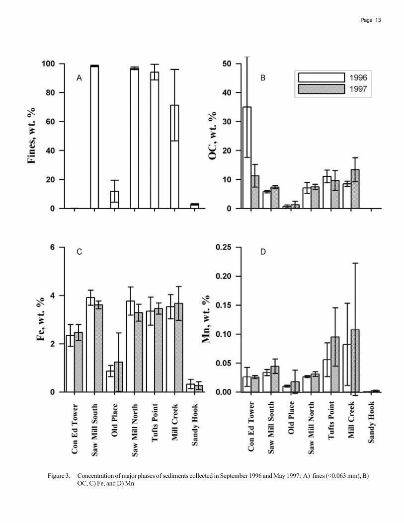
13Page

Figure 3. Concentration of major phases of sediments collected in September 1996 and May 1997: A) fines (<0.063 mm), B)OC, C) Fe, and D) Mn.

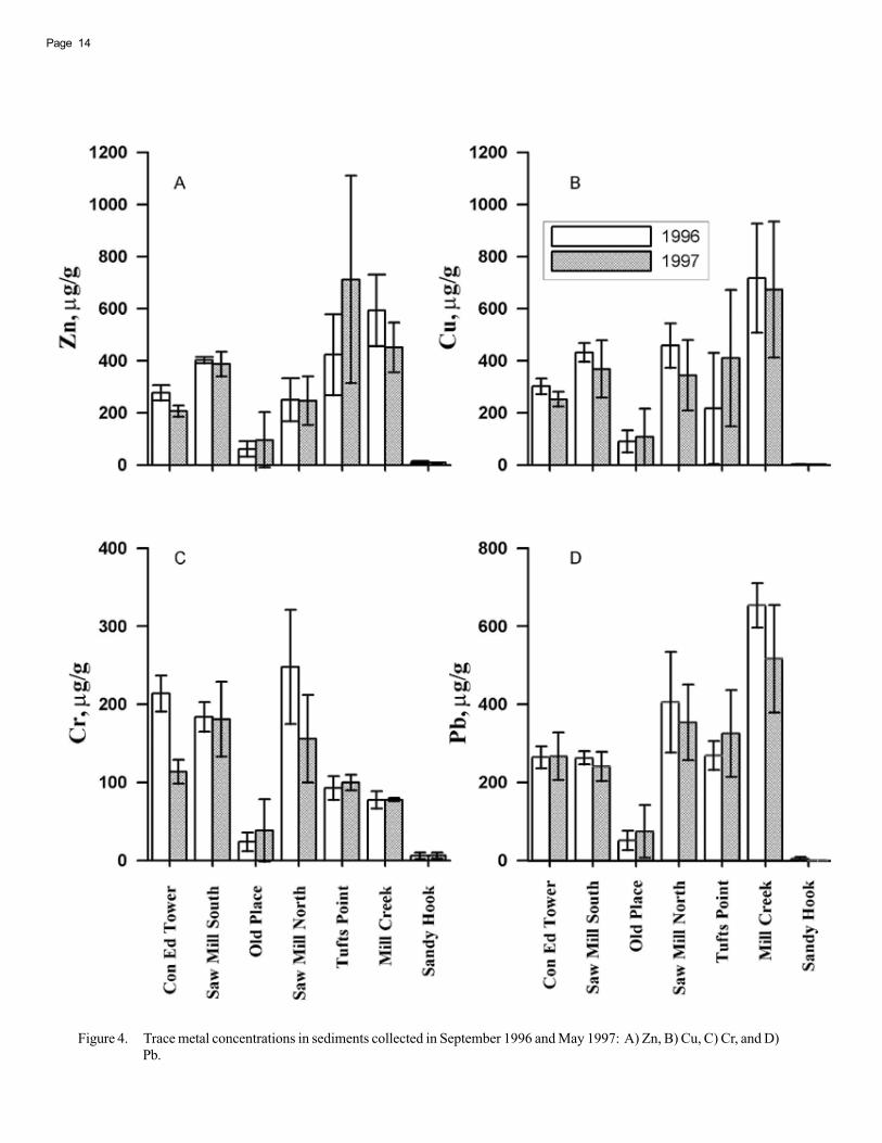
Page 14

Figure 4. Trace metal concentrations in sediments collected in September 1996 and May 1997: A) Zn, B) Cu, C) Cr, and D)Pb.

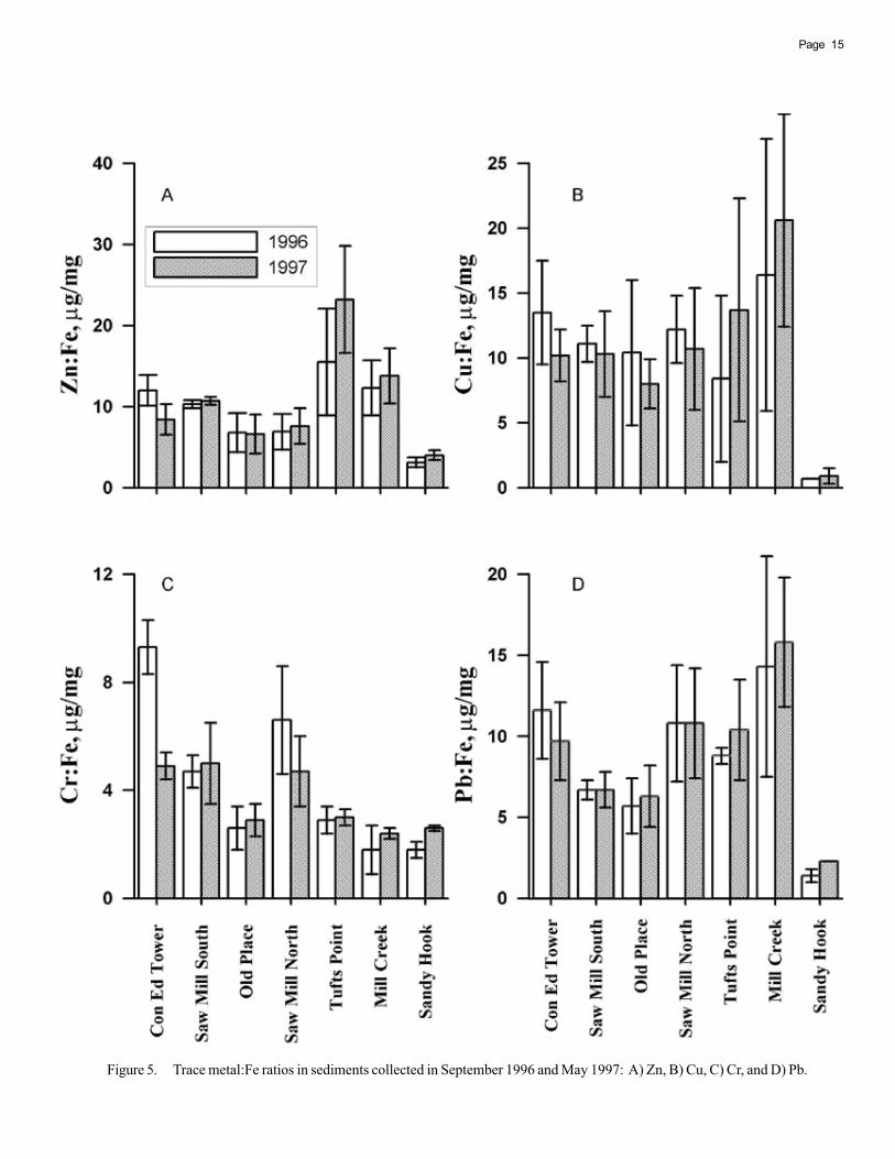
15Page

Figure 5. Trace metal:Fe ratios in sediments collected in September 1996 and May 1997: A) Zn, B) Cu, C) Cr, and D) Pb.

Page 16

Figure 6. Concentrations in mussels collected in September 1996 and May 1997 for the metals exhibiting the greatestseasonal differences: A) Ni, B) Cr, C) Hg, and D) Ag.

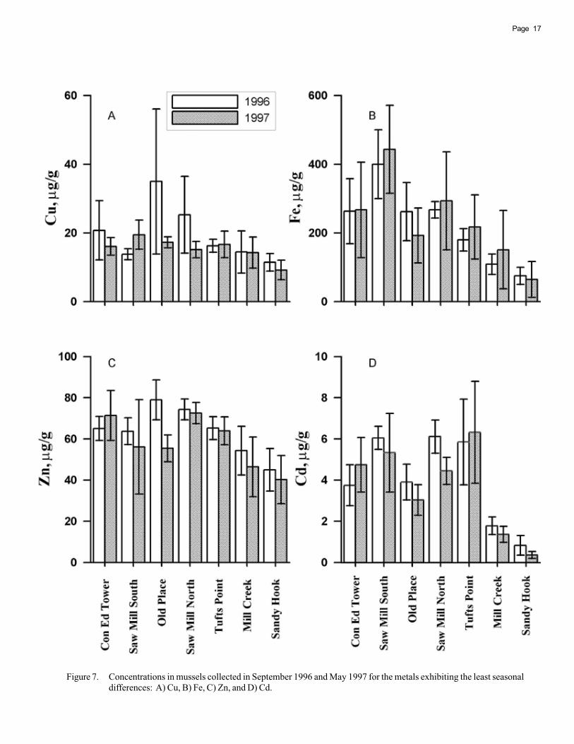
17Page

Figure 7. Concentrations in mussels collected in September 1996 and May 1997 for the metals exhibiting the least seasonaldifferences: A) Cu, B) Fe, C) Zn, and D) Cd.

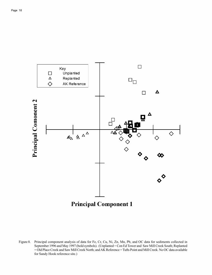
Page 18

Figure 8. Principal component analysis of data for Fe, Cr, Cu, Ni, Zn, Mn, Pb, and OC data for sediments collected inSeptember 1996 and May 1997 (bold symbols). (Unplanted = Con Ed Tower and Saw Mill Creek South; Replanted= Old Place Creek and Saw Mill Creek North; and AK Reference = Tufts Point and Mill Creek. No OC data availablefor Sandy Hook reference site.)

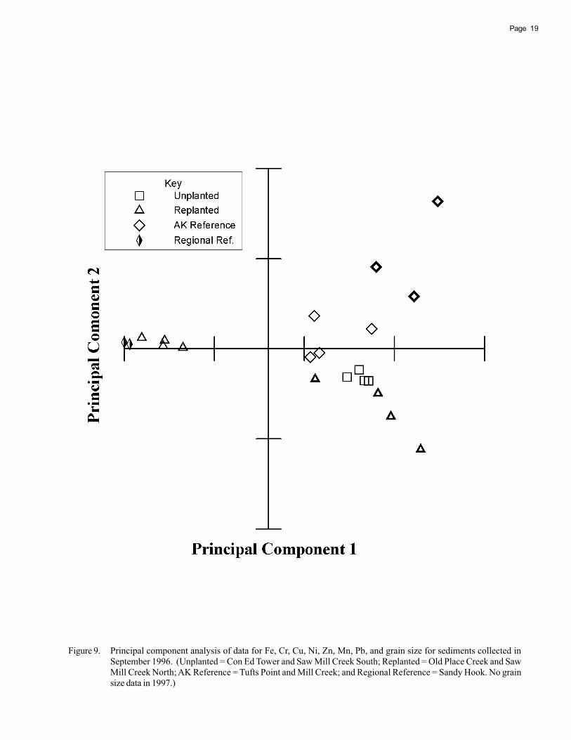
19Page

Figure 9. Principal component analysis of data for Fe, Cr, Cu, Ni, Zn, Mn, Pb, and grain size for sediments collected inSeptember 1996. (Unplanted = Con Ed Tower and Saw Mill Creek South; Replanted = Old Place Creek and SawMill Creek North; AK Reference = Tufts Point and Mill Creek; and Regional Reference = Sandy Hook. No grainsize data in 1997.)

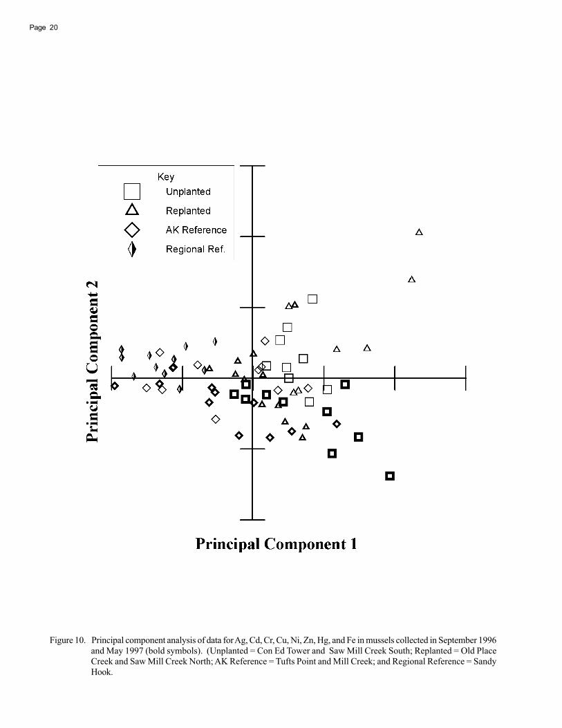
Page 20

Figure 10. Principal component analysis of data for Ag, Cd, Cr, Cu, Ni, Zn, Hg, and Fe in mussels collected in September 1996and May 1997 (bold symbols). (Unplanted = Con Ed Tower and Saw Mill Creek South; Replanted = Old PlaceCreek and Saw Mill Creek North; AK Reference = Tufts Point and Mill Creek; and Regional Reference = SandyHook.

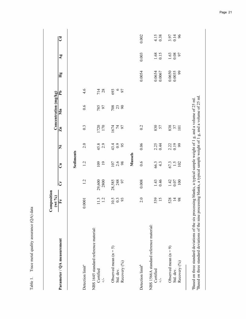
Tabl

e 1.

Trac

e m

etal

qua

lity

assu

ranc

e (Q

A) d

ata

Com

posit

ion

(wt %

)C

once

ntra

tion

(mg/

kg)

Para

met

er /

QA

mea

sure

men

tFe

Cr

Cu

Ni

ZnM

nPb

Hg

Ag

Cd

Sedi

men

ts

Det

ectio

n lim

ita0.

0001

1.2

1.2

2.0

0.3

0.6

4.6

NB

S 16

45 st

anda

rd re

fere

nce

mat

eria

l:C

ertif

ied

11.3

29,6

0010

945

.817

2078

571

4+/

-1.

228

0019

2.9

170

9728

Obs

erve

d m

ean

(n =

5)

10.5

28,5

8510

743

.416

7470

869

3St

d. d

ev.

0.3

248

2.6

0.9

7423

6R

ecov

ery

(%)

9397

9895

9790

97

Mus

sels

Det

ectio

n lim

itb2.

00.

008

0.6

0.06

0.2

0.00

540.

003

0.00

2

NB

S 15

66A

stan

dard

refe

renc

e m

ater

ial:

Cer

tifie

d53

91.

4366

.32.

2583

00.

0654

1.68

4.15

+/-

150.

464.

30.

4457

0.00

670.

150.

38

Obs

erve

d m

ean

(n =

9)

528

1.42

67.3

2.22

838

0.06

501.

633.

97St

d. d

ev.

140.

071.

50.

1937

0.00

350.

080.

14R

ecov

ery

(%)

9810

010

299

101

9997

96

a Bas

ed o

n th

ree

stan

dard

dev

iatio

ns o

f the

six

proc

essi

ng b

lank

s, a

typi

cal s

ampl

e w

eigh

t of 1

g, a

nd a

vol

ume

of 2

5 m

l.b B

ased

on

thre

e st

anda

rd d

evia

tions

of t

he n

ine

proc

essi

ng b

lank

s, a

typi

cal s

ampl

e w

eigh

t of 1

g, a

nd a

vol

ume

of 2

5 m

l.

21Page

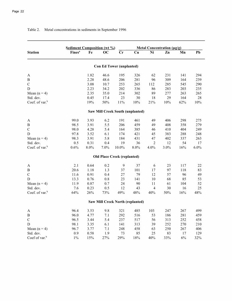
Table 2. Metal concentrations in sediments in September 1996

Sediment Composition (wt %) Metal Concentration (μg/g)

Station Fines Fe OC Cr Cu Ni Zn Mn Pba

Con Ed Tower (unplanted)

A 1.82 46.6 195 326 62 231 141 294

B 2.28 48.6 206 281 96 309 164 239

C 3.08 10.7 253 265 112 285 545 290

D 2.23 34.2 202 336 86 283 203 235

Mean (n = 4) 2.35 35.0 214 302 89 277 263 265

Std. dev. 0.45 17.4 23 30 18 29 164 28

Coef. of var. 19% 50% 11% 10% 21% 10% 62% 10%b

Saw Mill Creek South (unplanted)

A 99.0 3.93 6.2 191 461 49 406 298 275

B 98.5 3.91 5.5 206 459 49 408 358 279

C 98.0 4.28 5.4 164 385 46 410 404 249

D 97.8 3.52 6.1 174 421 45 383 288 248

Mean (n = 4) 98.3 3.91 5.8 184 431 47 402 337 263

Std. dev. 0.5 0.31 0.4 19 36 2 12 54 17

Coef. of var. 0.6% 8.0% 7.0% 10.0% 8.0% 4.0% 3.0% 16% 6.0%b

Old Place Creek (replanted)

A 2.1 0.64 0.2 9 37 6 23 117 22

B 20.6 1.18 1.3 37 101 17 97 118 83

C 11.6 0.91 0.4 27 79 12 57 96 49

D 13.3 0.76 0.8 23 141 10 68 85 53

Mean (n = 4) 11.9 0.87 0.7 24 90 11 61 104 52

Std. dev. 7.6 0.23 0.5 12 43 4 30 16 25

Coef. of var. 64% 26% 73% 49% 48% 40% 50% 16% 48%b

Saw Mill Creek North (replanted)

A 96.4 3.53 9.8 321 485 103 247 267 499

B 96.0 4.77 7.1 292 516 53 186 281 459

C 96.5 3.44 5.4 237 517 56 313 252 458

D 98.1 3.35 6.1 141 313 39 252 270 210

Mean (n = 4) 96.7 3.77 7.1 248 458 63 250 267 406

Std. dev. 0.9 0.58 1.9 73 85 25 83 17 129

Coef of var. 1% 15% 27% 29% 18% 40% 33% 6% 32%b

Page 22

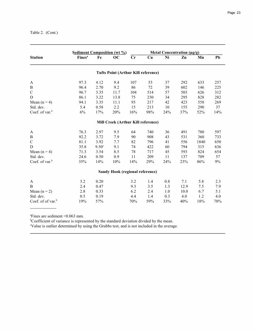
Table 2. (Cont.)

Sediment Composition (wt %) Metal Concentration (μg/g)

Station Fines Fe OC Cr Cu Ni Zn Mn Pba

Tufts Point (Arthur Kill reference)

A 97.3 4.12 9.4 107 53 37 292 633 257

B 96.4 2.70 9.2 86 72 39 602 146 225

C 96.7 3.35 11.7 104 514 57 503 626 312

D 86.1 3.22 13.8 75 230 34 295 828 282

Mean (n = 4) 94.1 3.35 11.1 93 217 42 423 558 269

Std. dev. 5.4 0.58 2.2 15 213 10 155 290 37

Coef. of var. 6% 17% 20% 16% 98% 24% 37% 52% 14%b

Mill Creek (Arthur Kill reference)

A 76.3 2.97 9.5 64 740 36 491 780 597

B 92.2 3.72 7.9 90 908 43 531 360 733

C 81.1 3.92 7.7 82 796 41 556 1840 650

D 35.8 9.50 9.1 74 422 60 794 315 636c

Mean (n = 4) 71.3 3.54 8.5 78 717 45 593 824 654

Std. dev. 24.6 0.50 0.9 11 209 11 137 709 57

Coef. of var. 35% 14% 10% 14% 29% 24% 23% 86% 9%b

Sandy Hook (regional reference)

A 3.2 0.20 3.2 1.4 0.8 7.1 5.8 2.3

B 2.4 0.47 9.3 3.5 1.3 12.9 7.5 7.9

Mean (n = 2) 2.8 0.33 6.2 2.4 1.0 10.0 6.7 5.1

Std. dev. 0.5 0.19 4.4 1.4 0.3 4.0 1.2 4.0

Coef. of of var. 19% 57% 70% 59% 33% 40% 18% 78%b

Fines are sediment <0.063 mm.a

Coefficient of variance is represented by the standard deviation divided by the mean.b

Value is outlier determined by using the Grubbs test, and is not included in the average.c

23Page

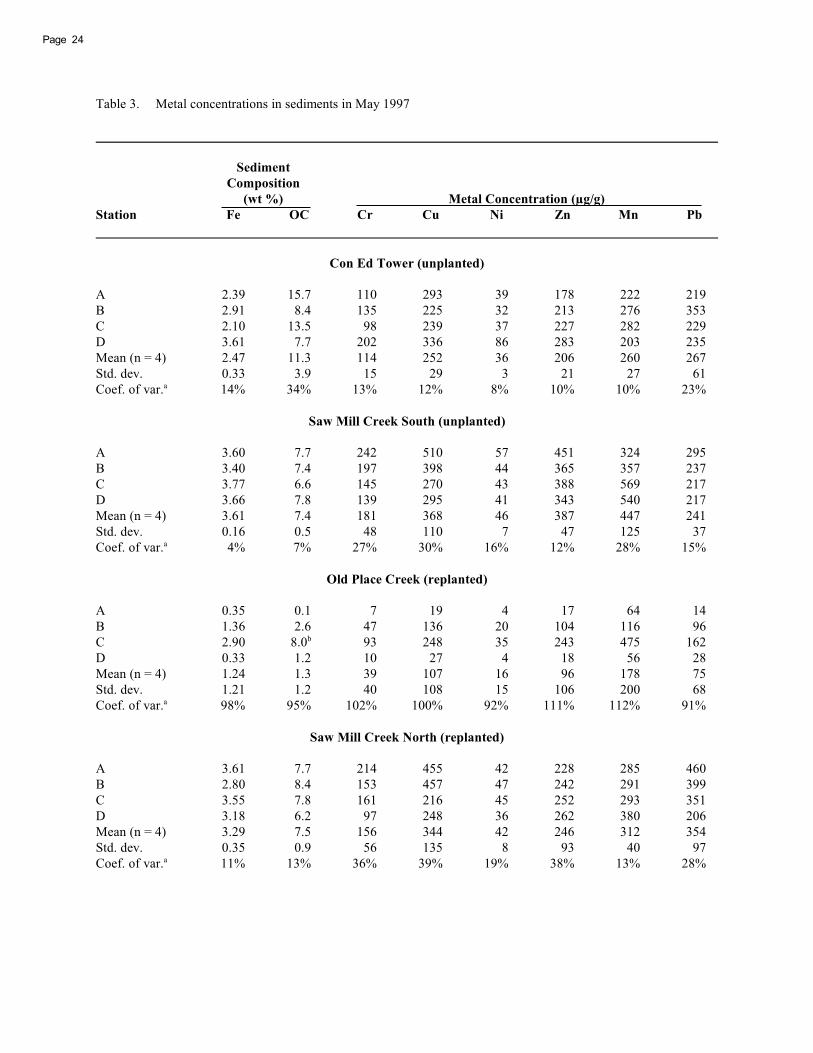
Table 3. Metal concentrations in sediments in May 1997

Sediment

Composition

(wt %) Metal Concentration (μg/g)

Station Fe OC Cr Cu Ni Zn Mn Pb

Con Ed Tower (unplanted)

A 2.39 15.7 110 293 39 178 222 219

B 2.91 8.4 135 225 32 213 276 353

C 2.10 13.5 98 239 37 227 282 229

D 3.61 7.7 202 336 86 283 203 235

Mean (n = 4) 2.47 11.3 114 252 36 206 260 267

Std. dev. 0.33 3.9 15 29 3 21 27 61

Coef. of var. 14% 34% 13% 12% 8% 10% 10% 23%a

Saw Mill Creek South (unplanted)

A 3.60 7.7 242 510 57 451 324 295

B 3.40 7.4 197 398 44 365 357 237

C 3.77 6.6 145 270 43 388 569 217

D 3.66 7.8 139 295 41 343 540 217

Mean (n = 4) 3.61 7.4 181 368 46 387 447 241

Std. dev. 0.16 0.5 48 110 7 47 125 37

Coef. of var. 4% 7% 27% 30% 16% 12% 28% 15%a

Old Place Creek (replanted)

A 0.35 0.1 7 19 4 17 64 14

B 1.36 2.6 47 136 20 104 116 96

C 2.90 8.0 93 248 35 243 475 162b

D 0.33 1.2 10 27 4 18 56 28

Mean (n = 4) 1.24 1.3 39 107 16 96 178 75

Std. dev. 1.21 1.2 40 108 15 106 200 68

Coef. of var. 98% 95% 102% 100% 92% 111% 112% 91%a

Saw Mill Creek North (replanted)

A 3.61 7.7 214 455 42 228 285 460

B 2.80 8.4 153 457 47 242 291 399

C 3.55 7.8 161 216 45 252 293 351

D 3.18 6.2 97 248 36 262 380 206

Mean (n = 4) 3.29 7.5 156 344 42 246 312 354

Std. dev. 0.35 0.9 56 135 8 93 40 97

Coef. of var. 11% 13% 36% 39% 19% 38% 13% 28%a

Page 24

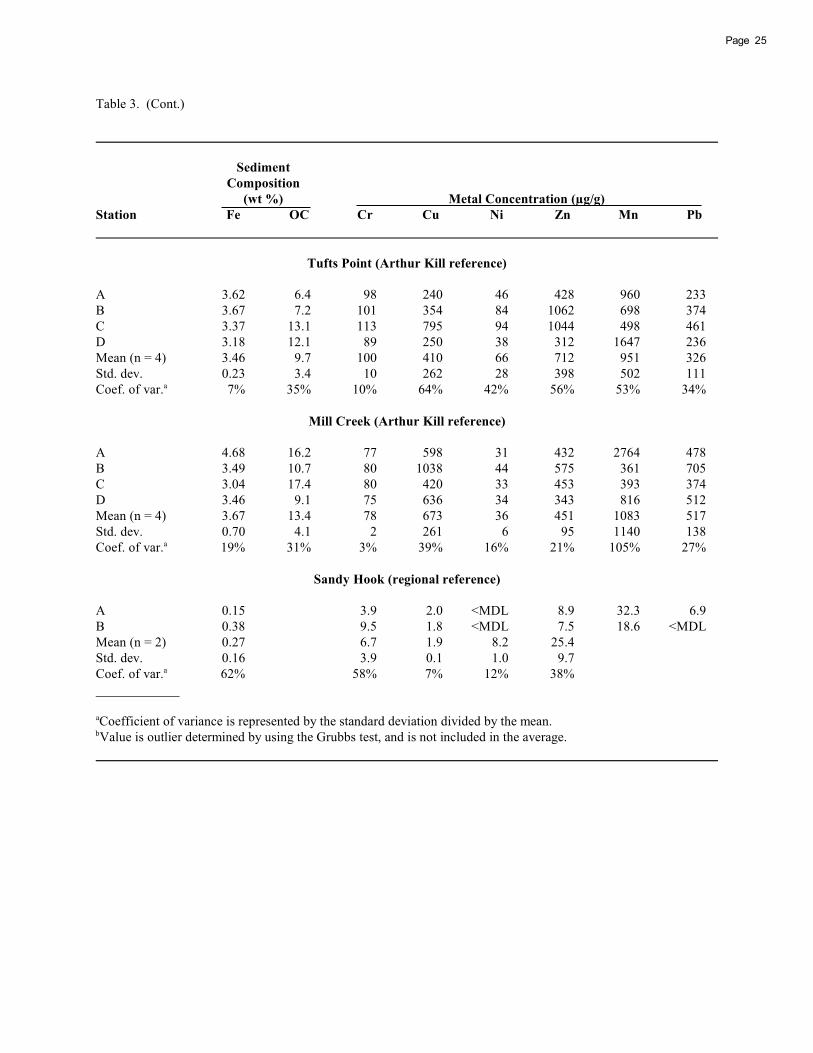
Table 3. (Cont.)

Sediment

Composition

(wt %) Metal Concentration (μg/g)

Station Fe OC Cr Cu Ni Zn Mn Pb

Tufts Point (Arthur Kill reference)

A 3.62 6.4 98 240 46 428 960 233

B 3.67 7.2 101 354 84 1062 698 374

C 3.37 13.1 113 795 94 1044 498 461

D 3.18 12.1 89 250 38 312 1647 236

Mean (n = 4) 3.46 9.7 100 410 66 712 951 326

Std. dev. 0.23 3.4 10 262 28 398 502 111

Coef. of var. 7% 35% 10% 64% 42% 56% 53% 34%a

Mill Creek (Arthur Kill reference)

A 4.68 16.2 77 598 31 432 2764 478

B 3.49 10.7 80 1038 44 575 361 705

C 3.04 17.4 80 420 33 453 393 374

D 3.46 9.1 75 636 34 343 816 512

Mean (n = 4) 3.67 13.4 78 673 36 451 1083 517

Std. dev. 0.70 4.1 2 261 6 95 1140 138

Coef. of var. 19% 31% 3% 39% 16% 21% 105% 27%a

Sandy Hook (regional reference)

A 0.15 3.9 2.0 <MDL 8.9 32.3 6.9

B 0.38 9.5 1.8 <MDL 7.5 18.6 <MDL

Mean (n = 2) 0.27 6.7 1.9 8.2 25.4

Std. dev. 0.16 3.9 0.1 1.0 9.7

Coef. of var. 62% 58% 7% 12% 38%a

Coefficient of variance is represented by the standard deviation divided by the mean.a

Value is outlier determined by using the Grubbs test, and is not included in the average.b

25Page

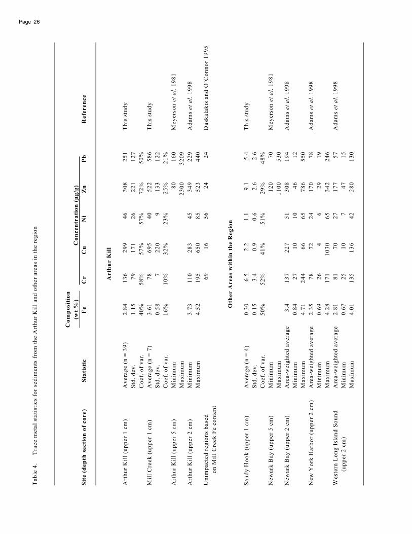
Ta

ble

4.

Tra

ce

me

tal

sta

tist

ics

for

sed

ime

nts

fro

m t

he

Art

hu

r K

ill

an

d o

the

r are

as

in t

he

reg

ion

Co

mp

osi

tio

n

(wt

%)

Co

nce

ntr

ati

on

(μ

g/g

)

Sit

e (

dep

th s

ecti

on

of

co

re)

Sta

tist

icF

eC

rC

uN

iZ

nP

bR

efe

ren

ce

Arth

ur K

ill

Art

hu

r K

ill

(up

pe

r 1

cm

)A

vera

ge

(n =

39

)2

.84

13

62

99

46

30

82

51

Th

is s

tud

y

Std

. d

ev

.1

.15

79

17

12

62

21

12

7

Co

ef.

of

va

r.4

0%

58

%5

7%

57

%7

2%

50

%

Mil

l C

reek

(u

pp

er

1 c

m)

Av

era

ge

(n =

7)

3.6

17

86

95

40

52

25

86

Th

is s

tud

y

Std

. d

ev

.0

.58

72

20

91

33

12

2

Co

ef.

of

va

r.1

6%

10

%3

2%

23

%2

5%

21

%

Art

hu

r K

ill

(up

per

5 c

m)

Min

imu

m8

01

60

Mey

ers

on

et

al.

19

81

Ma

xim

um

23

00

32

09

Art

hu

r K

ill

(up

per

2 c

m)

Min

imu

m3

.73

11

02

83

45

34

92

29

Ad

am

set

al.

19

98

Ma

xim

um

4.5

21

95

65

08

55

23

44

0

Un

imp

acte

dre

gio

ns

base

d6

91

65

62

42

4D

ask

ala

kis

an

d O

’Co

nn

or

19

95

on

Mil

l C

reek

Fe c

on

ten

t

Oth

er

Ar

ea

s w

ith

in t

he R

eg

ion

San

dy

Ho

ok

(u

pp

er

1 c

m)

Av

era

ge

(n =

4)

0.3

06

.52

.21

.19

.15

.4T

his

stu

dy

Std

. d

ev

.0

.15

3.4

0.9

0.6

2.6

2.6

Co

ef.

of

va

r.5

0%

52

%4

1%

51

%2

9%

48

%

New

ark

Bay

(up

per

5 c

m)

Min

imu

m1

20

70

Mey

ers

on

et

al.

19

81

Ma

xim

um

11

00

53

0

New

ark

Bay

(u

pp

er

2 c

m)

Are

a-w

eig

hte

d a

vera

ge

3.4

13

72

27

51

30

81

94

Ad

am

set

al.

19

98

Min

imu

m0

.84

27

10

10

46

12

Ma

xim

um

4.7

12

44

66

65

78

65

50

New

Yo

rk H

arb

or

(up

per

2 c

m)

Are

a-w

eig

hte

d a

vera

ge

2.3

57

87

22

41

70

78

Ad

am

set

al.

19

98

Min

imu

m0

.69

26

46

29

19

Ma

xim

um

4.2

81

71

10

30

65

34

22

46

West

ern

Lo

ng

Isl

an

d S

ou

nd

Are

a-w

eig

hte

d a

vera

ge

2.8

18

17

02

71

77

57

Ad

am

set

al.

19

98

(u

pp

er

2 c

m)

Min

imu

m0

.67

25

10

74

71

5

Ma

xim

um

4.0

11

35

13

64

22

80

13

0

Page 26

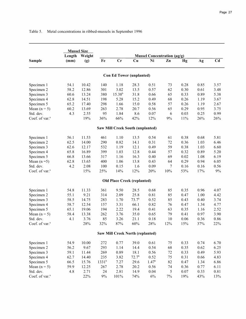
Table 5. Metal concentrations in ribbed-mussels in September 1996

Mussel Size

Length Weight Mussel Concentration (μg/g)

Sample (mm) (g) Fe Cr Cu Ni Zn Hg Ag Cd

Con Ed Tower (unplanted)

Specimen 1 54.1 10.42 140 1.18 28.3 0.51 73 0.28 0.85 3.57

Specimen 2 58.2 12.86 301 3.02 13.5 0.57 62 0.30 0.61 3.48

Specimen 3 60.6 13.24 380 15.38 31.8 0.66 65 0.33 0.89 5.38b

Specimen 4 62.8 14.51 198 5.28 15.2 0.49 68 0.26 1.19 3.67

Specimen 5 65.2 17.40 298 1.66 15.0 0.58 57 0.26 1.19 2.67

Mean (n = 5) 60.2 13.69 263 2.78 20.7 0.56 65 0.29 0.95 3.75

Std. dev. 4.3 2.55 95 1.84 8.6 0.07 6 0.03 0.25 0.99

Coef. of var. 19% 36% 66% 42% 12% 9% 11% 26% 26%a

Saw Mill Creek South (unplanted)

Specimen 1 56.1 11.53 461 1.10 13.5 0.54 61 0.38 0.68 5.81

Specimen 2 62.5 14.00 290 0.82 14.1 0.31 72 0.36 1.03 6.46

Specimen 3 62.6 12.17 532 1.19 12.1 0.49 59 0.38 1.03 6.60

Specimen 4 65.8 16.89 399 1.03 12.8 0.44 57 0.32 0.89 5.20

Specimen 5 66.8 13.66 317 1.16 16.3 0.40 69 0.02 1.08 6.19

Mean (n =5) 62.8 13.65 400 1.06 13.8 0.43 64 0.29 0.94 6.05

Std. dev. 4.2 2.08 100 0.15 1.6 0.09 7 0.16 0.16 0.56

Coef. of var. 15% 25% 14% 12% 20% 10% 53% 17% 9%a

Old Place Creek (replanted)

Specimen 1 54.8 11.33 361 9.50 28.5 0.68 85 0.35 0.96 4.07

Specimen 2 55.1 9.21 314 2.09 25.8 0.81 85 0.47 1.00 4.42

Specimen 3 58.5 14.75 283 1.70 73.7 0.52 85 0.43 0.40 3.74b

Specimen 4 58.7 12.54 157 3.31 66.1 0.82 76 0.47 1.34 4.77

Specimen 5 65.1 19.06 194 2.22 19.4 0.41 63 0.35 1.16 2.52

Mean (n = 5) 58.4 13.38 262 3.76 35.0 0.65 79 0.41 0.97 3.90

Std. dev. 4.1 3.76 85 3.26 21.1 0.18 10 0.06 0.36 0.86

Coef. of var. 28% 32% 87% 60% 28% 12% 15% 37% 22%a

Saw Mill Creek North (replanted)

Specimen 1 54.9 10.00 272 0.77 39.0 0.61 75 0.33 0.74 6.70

Specimen 2 56.2 9.67 293 1.14 14.4 0.54 68 0.35 0.62 6.25

Specimen 3 59.1 11.44 269 0.89 18.1 0.56 72 0.33 0.49 5.93

Specimen 4 62.7 14.40 235 3.82 72.7 0.52 75 0.31 0.66 4.83b

Specimen 5 66.5 15.76 1331 7.27 29.6 1.47 82 0.47 1.34 6.86b b

Mean (n = 5) 59.9 12.25 267 2.78 20.2 0.56 74 0.36 0.77 6.11

Std. dev. 4.8 2.71 24 2.81 14.9 0.04 5 0.07 0.33 0.81

Coef. of var. 22% 9% 101% 74% 6% 7% 19% 43% 13%a

27Page

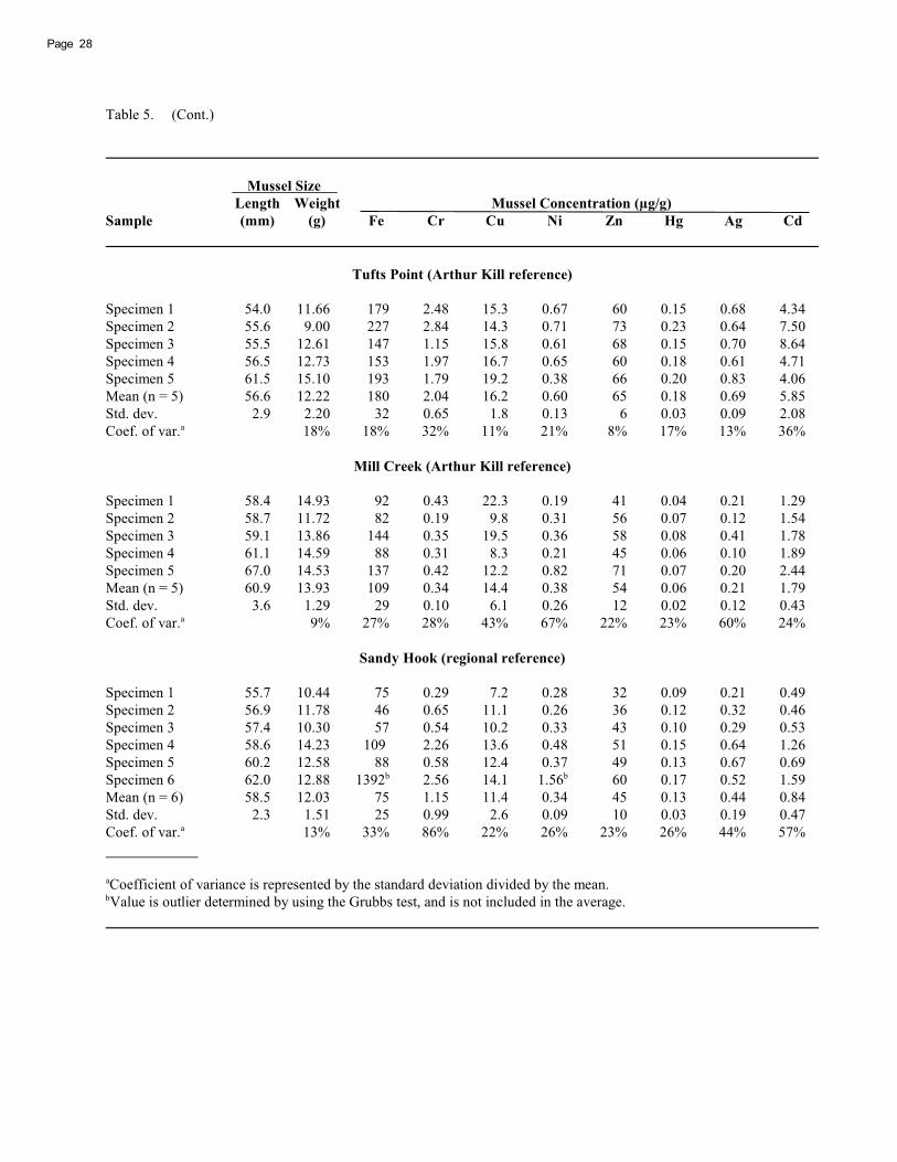
Table 5. (Cont.)

Mussel Size

Length Weight Mussel Concentration (μg/g)

Sample (mm) (g) Fe Cr Cu Ni Zn Hg Ag Cd

Tufts Point (Arthur Kill reference)

Specimen 1 54.0 11.66 179 2.48 15.3 0.67 60 0.15 0.68 4.34

Specimen 2 55.6 9.00 227 2.84 14.3 0.71 73 0.23 0.64 7.50

Specimen 3 55.5 12.61 147 1.15 15.8 0.61 68 0.15 0.70 8.64

Specimen 4 56.5 12.73 153 1.97 16.7 0.65 60 0.18 0.61 4.71

Specimen 5 61.5 15.10 193 1.79 19.2 0.38 66 0.20 0.83 4.06

Mean (n = 5) 56.6 12.22 180 2.04 16.2 0.60 65 0.18 0.69 5.85

Std. dev. 2.9 2.20 32 0.65 1.8 0.13 6 0.03 0.09 2.08

Coef. of var. 18% 18% 32% 11% 21% 8% 17% 13% 36%a

Mill Creek (Arthur Kill reference)

Specimen 1 58.4 14.93 92 0.43 22.3 0.19 41 0.04 0.21 1.29

Specimen 2 58.7 11.72 82 0.19 9.8 0.31 56 0.07 0.12 1.54

Specimen 3 59.1 13.86 144 0.35 19.5 0.36 58 0.08 0.41 1.78

Specimen 4 61.1 14.59 88 0.31 8.3 0.21 45 0.06 0.10 1.89

Specimen 5 67.0 14.53 137 0.42 12.2 0.82 71 0.07 0.20 2.44

Mean (n = 5) 60.9 13.93 109 0.34 14.4 0.38 54 0.06 0.21 1.79

Std. dev. 3.6 1.29 29 0.10 6.1 0.26 12 0.02 0.12 0.43

Coef. of var. 9% 27% 28% 43% 67% 22% 23% 60% 24%a

Sandy Hook (regional reference)

Specimen 1 55.7 10.44 75 0.29 7.2 0.28 32 0.09 0.21 0.49

Specimen 2 56.9 11.78 46 0.65 11.1 0.26 36 0.12 0.32 0.46

Specimen 3 57.4 10.30 57 0.54 10.2 0.33 43 0.10 0.29 0.53

Specimen 4 58.6 14.23 109 2.26 13.6 0.48 51 0.15 0.64 1.26

Specimen 5 60.2 12.58 88 0.58 12.4 0.37 49 0.13 0.67 0.69

Specimen 6 62.0 12.88 1392 2.56 14.1 1.56 60 0.17 0.52 1.59b b

Mean (n = 6) 58.5 12.03 75 1.15 11.4 0.34 45 0.13 0.44 0.84

Std. dev. 2.3 1.51 25 0.99 2.6 0.09 10 0.03 0.19 0.47

Coef. of var. 13% 33% 86% 22% 26% 23% 26% 44% 57%a

Coefficient of variance is represented by the standard deviation divided by the mean.a

Value is outlier determined by using the Grubbs test, and is not included in the average.b

Page 28

Table 6. Metal concentrations in ribbed-mussels in May 1997

Mussel Size

Length Weight Mussel Concentration (μg/g)

Sample (mm) (g) Fe Cr Cu Ni Zn Hg Ag Cd

Con Ed Tower (unplanted)

Specimen 1 56.6 11.15 952 3.27 49.3 1.65 94 0.36 2.25 12.22b b b b b b b b b b

Specimen 2 57.7 12.15 465 1.93 18.5 1.20 83 0.26 0.20 4.56

Specimen 3 58.7 14.00 228 1.02 16.6 0.55 58 0.21 0.23 3.04

Specimen 4 59.9 13.51 235 0.80 16.8 0.49 80 0.18 0.45 5.21

Specimen 5 61.9 14.43 140 0.80 12.5 0.52 65 0.19 0.39 6.19

Specimen 6 62.2 15.44 1218 4.34 83.3 18.62 268 0.23 0.45 3.07b b b b b b b b b b

Mean (n = 4) 59.6 13.52 267 1.14 16.1 0.69 71 0.21 0.32 4.75

Std. dev. 1.8 0.99 139 0.54 2.5 0.34 12 0.19 0.36 4.81

Coef. of var. 7% 52% 47% 16% 49% 17% 92% 112% 101%a

Saw Mill Creek South (unplanted)

Specimen 1 56.9 9.26 681 1.94 12.9 1.17 74 0.41 0.50 8.52

Specimen 2 57.6 11.58 318 1.30 17.3 1.24 61 0.38 1.22 5.18

Specimen 3 59.1 13.75 369 0.94 23.4 0.99 55 0.22 0.55 2.97

Specimen 4 59.0 11.96 474 1.87 20.5 1.42 69 0.32 0.66 5.46

Specimen 5 60.7 15.15 384 1.38 24.5 0.78 11 0.23 0.52 3.93

Specimen 6 62.0 13.84 432 1.68 18.2 0.93 66 0.30 0.68 5.95

Mean (n = 6) 59.2 12.59 443 1.52 19.5 1.09 56 0.31 0.69 5.34

Std. dev. 1.9 2.10 128 0.38 4.3 0.23 23 0.08 0.27 1.91

Coef. of var. 17% 29% 25% 22% 21% 41% 25% 39% 36%a

Old Place Creek (replanted)

Specimen 1 55.3 14.38 196 1.93 16.4 0.70 64 0.22 0.54 3.26

Specimen 2 55.5 14.26 231 0.80 16.8 0.63 50 0.20 0.60 2.31

Specimen 3 55.0 12.61 145 1.12 19.3 0.54 63 0.30 1.55 4.09

Specimen 4 57.9 13.95 331 1.06 14.8 0.78 55 0.20 0.54 3.64

Specimen 5 58.8 15.78 134 1.35 18.3 0.57 52 0.27 0.46 2.51

Specimen 6 59.3 13.43 116 0.56 17.8 0.47 48 0.21 0.35 2.39

Mean (n = 6) 57.0 14.07 192 1.14 17.2 0.61 55 0.23 0.67 3.03

Std. dev. 1.9 1.06 80 0.47 1.6 0.11 7 0.04 0.44 0.74

Coef. of var. 8% 42% 42% 9% 18% 12% 18% 65% 25%a

Saw Mill Creek North (replanted)

Specimen 1 56.5 12.82 405 1.32 18.1 1.03 77 0.26 0.21 3.43

Specimen 2 57.9 13.41 249 0.95 13.0 0.88 79 0.24 0.41 4.91

Specimen 3 58.7 12.89 138 0.59 13.4 0.47 69 0.20 0.96 4.13

Specimen 4 62.6 13.83 491 1.68 16.5 0.63 72 0.29 0.25 5.33

Specimen 5 65.9 16.21 142 0.75 12.5 0.50 65 0.22 0.57 4.58

Specimen 6 65.7 16.44 333 1.29 17.1 0.64 73 0.22 0.36 4.30

Mean (n = 6) 61.2 14.27 293 1.10 15.1 0.69 73 0.24 0.46 4.45

Std. dev. 4.1 1.64 143 0.41 2.4 0.22 5 0.03 0.28 0.66

Coef. of var. 11% 49% 37% 16% 32% 7% 13% 60% 15%a

29Page

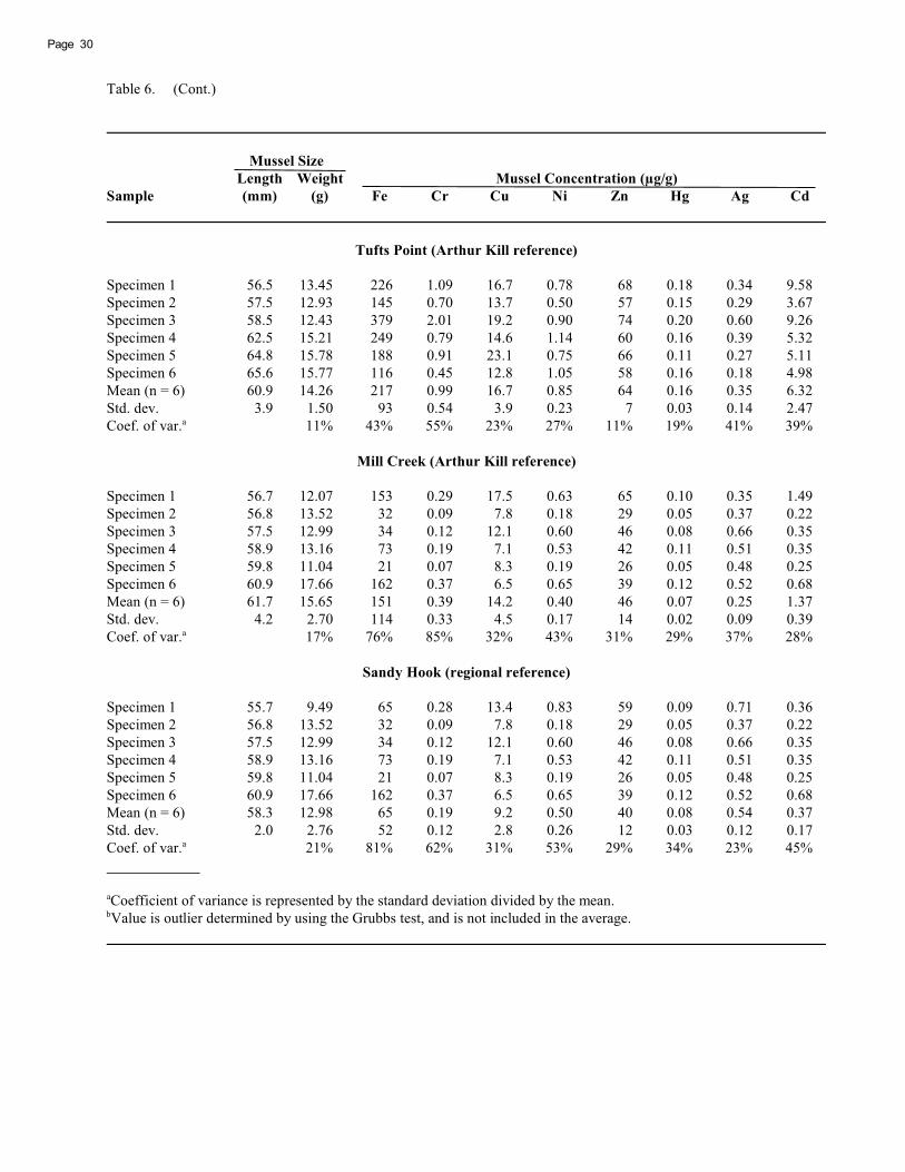
Table 6. (Cont.)

Mussel Size

Length Weight Mussel Concentration (μg/g)

Sample (mm) (g) Fe Cr Cu Ni Zn Hg Ag Cd

Tufts Point (Arthur Kill reference)

Specimen 1 56.5 13.45 226 1.09 16.7 0.78 68 0.18 0.34 9.58

Specimen 2 57.5 12.93 145 0.70 13.7 0.50 57 0.15 0.29 3.67

Specimen 3 58.5 12.43 379 2.01 19.2 0.90 74 0.20 0.60 9.26

Specimen 4 62.5 15.21 249 0.79 14.6 1.14 60 0.16 0.39 5.32

Specimen 5 64.8 15.78 188 0.91 23.1 0.75 66 0.11 0.27 5.11

Specimen 6 65.6 15.77 116 0.45 12.8 1.05 58 0.16 0.18 4.98

Mean (n = 6) 60.9 14.26 217 0.99 16.7 0.85 64 0.16 0.35 6.32

Std. dev. 3.9 1.50 93 0.54 3.9 0.23 7 0.03 0.14 2.47

Coef. of var. 11% 43% 55% 23% 27% 11% 19% 41% 39%a

Mill Creek (Arthur Kill reference)

Specimen 1 56.7 12.07 153 0.29 17.5 0.63 65 0.10 0.35 1.49

Specimen 2 56.8 13.52 32 0.09 7.8 0.18 29 0.05 0.37 0.22

Specimen 3 57.5 12.99 34 0.12 12.1 0.60 46 0.08 0.66 0.35

Specimen 4 58.9 13.16 73 0.19 7.1 0.53 42 0.11 0.51 0.35

Specimen 5 59.8 11.04 21 0.07 8.3 0.19 26 0.05 0.48 0.25

Specimen 6 60.9 17.66 162 0.37 6.5 0.65 39 0.12 0.52 0.68

Mean (n = 6) 61.7 15.65 151 0.39 14.2 0.40 46 0.07 0.25 1.37

Std. dev. 4.2 2.70 114 0.33 4.5 0.17 14 0.02 0.09 0.39

Coef. of var. 17% 76% 85% 32% 43% 31% 29% 37% 28%a

Sandy Hook (regional reference)

Specimen 1 55.7 9.49 65 0.28 13.4 0.83 59 0.09 0.71 0.36

Specimen 2 56.8 13.52 32 0.09 7.8 0.18 29 0.05 0.37 0.22

Specimen 3 57.5 12.99 34 0.12 12.1 0.60 46 0.08 0.66 0.35

Specimen 4 58.9 13.16 73 0.19 7.1 0.53 42 0.11 0.51 0.35

Specimen 5 59.8 11.04 21 0.07 8.3 0.19 26 0.05 0.48 0.25

Specimen 6 60.9 17.66 162 0.37 6.5 0.65 39 0.12 0.52 0.68

Mean (n = 6) 58.3 12.98 65 0.19 9.2 0.50 40 0.08 0.54 0.37

Std. dev. 2.0 2.76 52 0.12 2.8 0.26 12 0.03 0.12 0.17

Coef. of var. 21% 81% 62% 31% 53% 29% 34% 23% 45%a

Coefficient of variance is represented by the standard deviation divided by the mean.a

Value is outlier determined by using the Grubbs test, and is not included in the average.b

Page 30

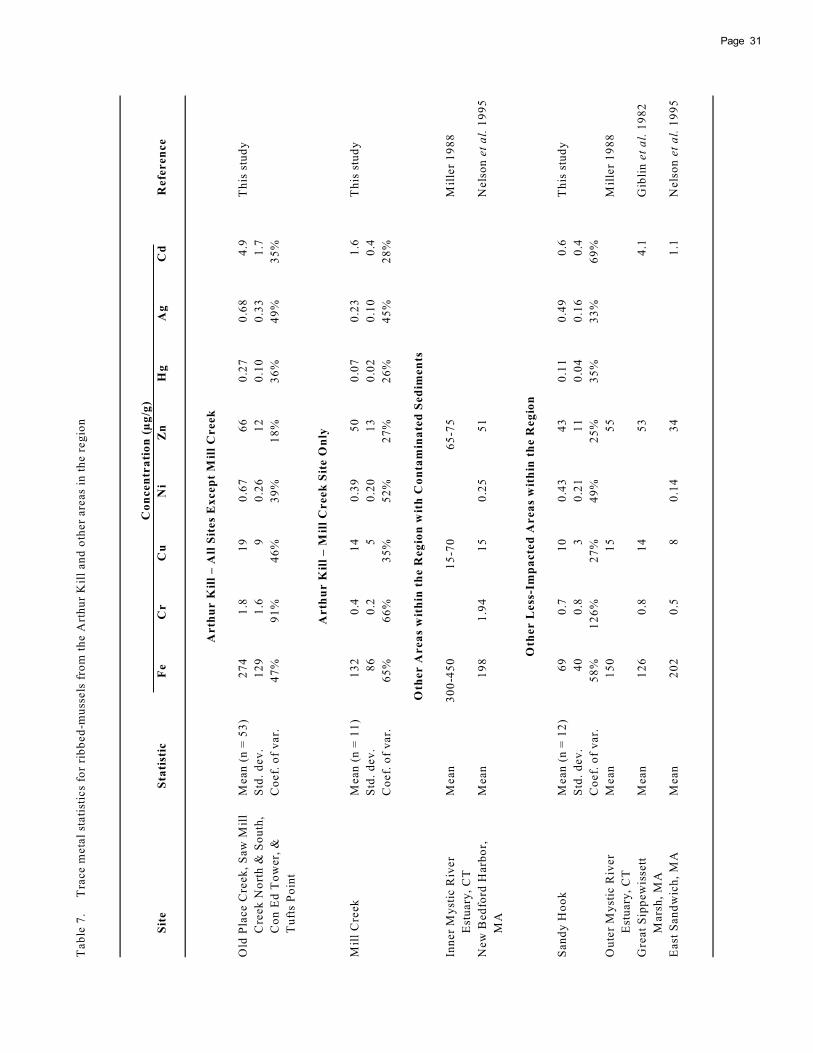
Ta

ble

7.

Tra

ce

me

tal

sta

tist

ics

for

rib

be

d-m

uss

els

fro

m t

he

Art

hu

r K

ill

an

d o

the

r are

as

in t

he

reg

ion

Co

nce

ntr

ati

on

(μ

g/g

)

Sit

eS

tati

stic

Fe

Cr

Cu

Ni

Zn

Hg

Ag

Cd

Refe

ren

ce

Arth

ur K

ill

– A

ll S

ites

Ex

cep

t M

ill

Creek

Old

Pla

ce

Cre

ek

, S

aw

Mil

lM

ean

(n

= 5

3)

27

41

.81

90

.67

66

0.2

70

.68

4.9

Th

is s

tud

y

Cre

ek

No

rth

& S

ou

th,

Std

. d

ev

.1

29

1.6

90

.26

12

0.1

00

.33

1.7

Co

n E

d T

ow

er,

&C

oe

f. o

f v

ar.

47

%9

1%

46

%3

9%

18

%3

6%

49

%3

5%

Tu

fts

Po

int

Arth

ur K

ill

– M

ill

Creek

Sit

e O

nly

Mil

l C

reek

Me

an

(n

= 1

1)

13

20

.41

40

.39

50

0.0

70

.23

1.6

Th

is s

tud

y

Std

. d

ev

.8

60

.25

0.2

01

30

.02

0.1

00

.4

Co

ef.

of

va

r.6

5%

66

%3

5%

52

%2

7%

26

%4

5%

28

%

Oth

er A

rea

sw

ith

in t

he R

eg

ion

wit

h C

on

tam

ina

ted

Sed

imen

ts

Inn

er

My

stic

Riv

er

Me

an

30

0-4

50

15

-70

65

-75

Mil

ler

19

88

Est

uary

, C

T

New

Bed

ford

Harb

or,

Mean

19

81

.94

15

0.2

55

1N

els

on

et

al.

19

95

MA

Oth

er

Le

ss-I

mp

acte

d A

rea

s w

ith

in t

he R

eg

ion

San

dy

Ho

ok

Me

an

(n

= 1

2)

69

0.7

10

0.4

34

30

.11

0.4

90

.6T

his

stu

dy

Std

. d

ev

.4

00

.83

0.2

11

10

.04

0.1

60

.4

Co

ef.

of

va

r.5

8%

12

6%

27

%4

9%

25

%3

5%

33

%6

9%

Ou

ter

My

stic

Riv

er

Me

an

15

01

55

5M

ille

r 1

98

8

Est

uary

, C

T

Gre

at

Sip

pew

isse

ttM

ean

12

60

.81

45

34

.1G

ibli

net

al.

19

82

Mars

h,

MA

East

San

dw

ich

, M

AM

ean

20

20

.58

0.1

43

41

.1N

els

on

et

al.

19

95

31Page

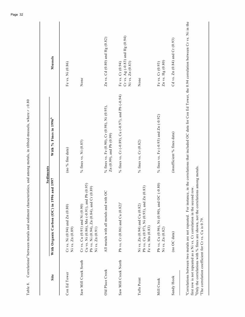
Tab

le 8

.C

orr

ela

tio

ns

betw

een

meta

ls a

nd

sed

imen

t ch

ara

cte

rist

ics,

an

d a

mo

ng

meta

ls,

in r

ibb

ed

-mu

ssels

, w

here

r�

0.8

0a

Se

dim

en

ts

Sit

eW

ith

Org

an

ic C

arb

on

(O

C)

in 1

99

6 a

nd

19

97

Wit

h %

Fin

es

in 1

99

6M

uss

els

b

Co

n E

d T

ow

er

Cr

vs.

Ni

(0.9

4)

an

d Z

n (

0.8

0)

(no

% f

ine

da

ta)

Fe v

s. N

i (0

.86

)

Ni

vs.

Zn

(0

.89

)

Sa

w M

ill

Cre

ek

So

uth

Cr

vs.

Cu

(0

.91

) an

d N

i (0

.90

)%

fin

es

vs.

Ni

(0.8

5)

No

ne

Cu

vs.

Ni

(0.8

6),

Mn

(-0

.91

), a

nd

Pb

(0

.95

)

Pb

vs.

Ni

(0.9

4),

Zn

(0

.84

), a

nd

Cr

(0.8

9)

Ni

vs.

Zn

(0

.91

)

Old

Pla

ce

Cre

ek

All

meta

ls w

ith

all

meta

ls a

nd

wit

h O

C%

fin

es

vs.

Fe (

0.9

0),

Cr

(0.9

8),

Ni

(0.9

5),

Zn

vs.

Cd

(0

.80

) an

d H

g (

0.8

2)

Zn

(0

.99

), a

nd

Pb

(0

.99

)

Saw

Mil

l C

reek

No

rth

Pb

vs.

Cr

(0.8

6)

an

d C

u (

0.8

2)

% f

ine

s v

s. C

r (-

0.8

9),

Cu

(-0

.97

), a

nd

Pb

(-0

.94

)F

e v

s. C

r (0

.94

)c

Cr

vs.

Ag

(-0

.83

) an

d H

g (

0.9

4)

Ni

vs.

Zn

(0

.83

)

Tu

fts

Po

int

Ni

vs.

Zn

(0

.94

) an

d C

u (

0.8

2)

% f

ines

vs.

Cr

(0.8

2)

No

ne

Pb

vs.

Cu

(0

.97

), N

i (0

.93

), a

nd

Zn

(0

.83

)

Fe v

s. M

n (

0.8

3)

Mil

l C

reek

Pb

vs.

Cu

(0

.96

), N

i (0

.90

), a

nd

OC

(-0

.80

)%

fin

es

vs.

Fe (

-0.9

3)

an

d Z

n (

-0.9

2)

Fe v

s. C

r (0

.93

)

Ni

vs.

Zn

(0

.82

)Z

n v

s. H

g (

0.8

0)

San

dy

Ho

ok

(no

OC

da

ta)

(in

suff

icie

nt

% f

ine

s d

ata

)C

d v

s. Z

n (

0.8

4)

an

d C

r (0

.93

)

Co

rrela

tio

ns

betw

een

tw

o m

eta

lsare

no

t re

pe

ate

d.

Fo

r in

stan

ce,

in t

he c

orr

ela

tio

ns

that

inclu

ded

OC

da

ta f

or

Co

n E

dT

ow

er,

th

e 0

.94

co

rrela

tio

n b

etw

een

Cr

vs.

Ni

in t

he

a firs

t ro

w i

s n

ot

rep

eate

d a

s a N

i v

s. C

r co

rrela

tio

n i

n t

he

seco

nd

ro

w.

On

ly t

he c

orr

ela

tio

ns

wit

h %

fin

es

are

sh

ow

n,

no

t th

e c

orr

ela

tio

ns

am

on

g m

eta

ls.

b Th

ec

orr

ela

tio

n c

oe

ffic

ien

t fo

r C

r v

s. C

u i

s 0

.79

.c

Page 32

33Page

III. PETROLEUM HYDROCARBONSIN SEDIMENTS AND RIBBED-MUSSELS (Geukensia demissa)

Ashok D. Deshpande9, 11, Bruce W. Dockum9, 12, and Amy M. Tesolin-Gee9, 10, 13

Postal Address: 9National Marine Fisheries Serv., 74 Magruder Rd., Highlands, NJ 07732Current Address: 10Dow Chemical Co., 2030 Dow Center, Midland, MI 48667E-Mail Addresses: 11Ashok.Deshpande@noaa.gov; 12Bruce.Dockum@noaa.gov; 13AMTesolin- Gee@dow.com

One surface sediment sample from Sandy Hook was col-lected during August 1997.

Mussel Collection, Processing, and Selection forAnalysis

Mussels were collected randomly at each site in theArthur Kill during September 1996 and May 1997. The num-ber of mussels available for collection varied by site andsampling period. Thus, 17-34 mussels were collected ateach site in September 1996, while only 6-15 mussels werecollected at each site in May 1997. Sandy Hook musselswere collected during February 1997.

Live mussels were brought to the Howard Laboratory,and placed overnight in a 4°C, temperature-controlled room.Material for the determination of method detection limits(MDLs) in the mussels was obtained by overnight depura-tion of 12 additional Sandy Hook mussels in aerated seawa-ter at 4°C. All mussels were dissected within 24 hr usingimplements cleaned with methylene chloride. After removalof extraneous materials from mussel shells (mud, barnacles,etc.), the physical characteristics were recorded for eachspecimen (Appendix Table B2). Mussel tissues were thenexcised, placed in precleaned glass containers, and archivedat the Howard Laboratory at -80°C.

The length of an individual mussel was assumed to berelated to its age, and possibly, the contaminant body bur-den. Since the length-frequency distribution of musselsvaried by site and sampling period (Figures 12 and 13), alength range of 55-74 mm (inclusive) -- visually identified tobe common to all sampling periods -- was selected as thebin range for analyses.

Five mussels at each site in the Arthur Kill were tar-geted for analyses. The bin range was divided into fivegroups (i.e., 55-58 mm, 59-62 mm, 63-66 mm, 67-70 mm, and71-74 mm), ensuring that mussels of different lengths wereincluded in the analyses. Each mussel was assigned a ran-dom number. Mussels with the highest random numberswere sequentially selected from each group. When therewere no mussels in one or more groups, mussels were se-lected in a two-step procedure. In step 1, the mussel withthe highest random number within each group containingmussels was selected. In step 2, the mussel with the high-est random number from all remaining mussels within the

INTRODUCTION

The goal of our study was to assess the effectivenessof the replanting effort for removing petroleum hydrocar-bon contaminants from the Arthur Kill marshes, and to as-sess the usefulness of ribbed-mussels as possiblebiomarkers of petroleum-related spills. Our field protocolincluded collection of sediment and ribbed-mussel samplesfrom the six saltmarsh sites in the Arthur Kill and from onesaltmarsh site on Sandy Hook (Appendix Table B1). Samplesfrom Sandy Hook provided a relatively uncontaminated re-gional reference for samples from the Arthur Kill marshes.

METHODS AND MATERIALS

Sediment Collection and Sectioning

Four stations were selected at each marsh site in theArthur Kill. Each station was located 0.2 m above the mid-tide, and the stations were spaced within 2-20 m of eachother (see description of the sampling transect in ChapterII, “Trace Metal Contaminants in Sediments and Ribbed-Mussels”). No cores were collected at the Sandy Hooksite. All sediment samples were archived at the HowardLaboratory either at -20°C or at -80°C.

During September 1996, one sediment core was takenby hand at each station using a chrome-plated copper tube(3.8-cm o.d. × 22.9-cm length). A total of 24 sediment cores(i.e., 6 sites × 4 stations per site × 1 core per station) werecollected. Sediment cores from Old Place Creek, Con EdTower, and Mill Creek were sectioned using a core-section-ing device built at the Howard Laboratory (Figure 11). Thecores contained large amounts of diverse plant and othermaterials that prevented precise sectioning. Each core wassectioned into five individual sections, with each sectionbeing approximately 1-cm thick and weighing approximately10 g. With four stations at each site and five sections percore per station, a total number of 60 core sections wereprepared for the three marsh sites.

Diverse plant and other materials in the sediments pre-vented precise sampling of the Arthur Kill surface sedi-ments. During May 1997, an approximately 1-cm section ofsurface sediment was collected at four stations at each ofthe six sites in the Arthur Kill using a stainless steel spoon.

Page 34

bin range was selected. Step 2 was repeated until the re-quirement of five mussels per site was met.

Seven out of the 12 undepurated mussels from SandyHook were targeted for analyses. The bin range was di-vided into seven groups (i.e., 55-56 mm, 57-58 mm, 59-60mm, 61-62 mm, 63-64 mm, 65-66 mm, and 67-68 mm), andrandom numbers were assigned to each mussel. Musselswith the highest random number in each group were se-lected for analysis.

Extraction of Hydrocarbons in Sediments

Twenty core sections each from Old Place Creek, ConEd Tower, and Mill Creek; four surface scoop samples eachfrom Old Place Creek and Con Ed Tower; and a single sur-face scoop sample from Sandy Hook were processed infour extraction batches (Appendix Table B3). All sedimentsamples were dried with sodium sulfate before extraction.In the first batch, we extracted the sediments by shakingthem with methylene chloride in an Erlenmeyer flask. Theshaking/extraction procedure was manual and laborious,and did not save as much on extraction time or glassware aswe initially thought. Therefore, Batches 2-4 samples wereextracted with methylene chloride using automated Soxhletextraction systems.

Batch 1 sediment samples were extracted by shakingsodium-sulfate-dried sediments with methylene chloride.Approximately 10 g of each Batch 1 sediment sample wereplaced into a mortar, then mixed by pestle with 60-80 g ofanhydrous sodium sulfate until the mixture was dry. Ap-proximately, 5 cc of activated copper were added to thesample for the bulk removal of elemental sulfur, and themixture was transferred to an Erlenmeyer flask. Surrogateinternal standard (20 μg of o-terphenyl) and any other spik-ing solutions, as appropriate, were added to the sample.Approximately 60 ml of methylene chloride were added tothe Erlenmeyer flask, and the sample was shaken overnight.Methylene chloride was decanted, and the procedure wasrepeated two more times. The combined extract was con-centrated to approximately 40 ml.

Batches 2-4 sediment samples were dried with sodiumsulfate, and extracted with a Soxhlet extraction apparatus.Approximately 10 g of each sample from Batches 2-4 wereplaced into a mortar, then mixed by pestle with 60-80 g ofanhydrous sodium sulfate until the mixture was dry. Thesample was then transferred to a cellulose thimble. Surro-gate internal standard (20 μg of o-terphenyl) and any otherspiking solutions, as appropriate, were added to the sample.The thimble was then transferred to a labeled Soxhlet ex-traction apparatus. Hydrocarbons were extracted with me-thylene chloride for 18-24 hr. Activated copper gauze wasplaced in the extraction apparatus for the bulk removal ofelemental sulfur. The methylene chloride extract was con-centrated to approximately 40 ml.

Initially, we experimented with the volume of concen-trate from each site to ensure that the flame ionization de-tector (FID) did not become overloaded during gas chro-matographic (GC) analyses. We assumed that all potentialinterfering compounds in the 40-ml extract were at a verylow level, and that they would not cause any chromato-graphic problems. Therefore, we injected 1 μL of this ex-tract directly into a gas chromatographic column withoutany additional cleanup. The samples in which hydrocar-bons were not detected were concentrated in a stepwisemanner until the hydrocarbons were detected. After com-pleting the screening of representative samples from eachsite, the methylene chloride extracts of all samples weresubjected to silica-alumina glass column chromatographicremoval of polar biogenic interferences. Column-cleanedextracts were then concentrated to appropriate final vol-umes for the GC analyses. GC internal standard (5-α-an-drostane) was added to each final extract before GC analy-ses.

Extraction of Hydrocarbons in Mussels

A total of 60 mussels from six Arthur Kill sites and sevenmussels from one Sandy Hook site were processed in threeextraction batches (Appendix Table B4).

Each mussel sample (3.2-15.4 g) was placed into a mor-tar, then mixed by pestle with 80 g of anhydrous sodiumsulfate until the mixture was dry. The sample was thentransferred to a cellulose thimble, and surrogate internalstandard (20 μg of o-terphenyl) and any other spiking solu-tions, as appropriate, were added to the sample. The thimblewas then transferred to a labeled Soxhlet extraction appara-tus. Hydrocarbons in mussels were extracted with methyl-ene chloride over 18-24 hr.

In Batch 1, we experimented with the volume of concen-trate to ensure that the FID did not become overloadedduring GC analyses. Initially, our total extract volume was50 ml, and we used 10 ml of this extract for the lipid determi-nation. We assumed that all potential interfering compoundsin the remaining 40 ml of extract were at a very low level, andthat they would not cause any chromatographic problems.Therefore, we injected 1 μL of this extract directly into theGC column without any additional cleanup. Contrary to ourexpectations based on the oil spill history in the Arthur Killmarshes, we barely observed any peaks in this dilute mus-sel extract. The remaining mussel extract was eluted througha silica-alumina glass column for the removal of polar lipidsand other polar biogenic interferences, and the sample wasconcentrated to a volume of 5 ml. Surprisingly, a 1-μL injec-tion of this extract did not overload the FID either, and thepeak sizes were still very minute. This initial work sug-gested that our standard protocol of concentrating thesample to a final volume of 1 ml was also suitable for ArthurKill and Sandy Hook mussels. All mussel extracts were

35Page

then subjected to silica-alumina glass column chromato-graphic cleanup. The column-cleaned extract was concen-trated to about 700-750 μL, the GC internal standard wasadded (200 μL of 5-α-androstane, 20 μg total), and the finalsample volume was brought to 1 ml using methylene chloride.

Gas Chromatographic Analyses of Hydrocarbons

Instrument Operating Parameters

Sediment and mussel samples were analyzed for a totalof 33 normal-chain hydrocarbons and two branched-chainhydrocarbons (Appendix Table B5) using a Hewlett Packard(HP) 5880A GC-FID. One microliter of the final sample ex-tract was injected into a fused silica capillary column insplitless mode using an HP 7673A autosampler. Extracts ofall mussel samples and extracts of sediment samples fromBatches 1, 2 (excluding the nine samples from Con Ed Tower),and 3 were injected into an HP-5 (0.32-mm i.d. × 30-m length× 0.25-μm film thickness) capillary column. Extracts of Batch2 sediment samples from the Con Ed Tower site and extractsof sediments from Batch 4 were injected into a J&W DB-5(0.45-mm i.d. × 30-m length × 0.42-μm film thickness) capil-lary column. The injector port temperature was set at 300°C,while the detector temperature was set at 280°C. An initialpurge time of 1 min was used to maximize the amount ofhigher-boiling hydrocarbons that reached the top of the GCcolumn. The column oven temperature was held at 50°C for1 min after sample injection, and then programmed to reach310°C at a rate of 3°C/min. The oven temperature was heldat the final temperature of 310°C for 30 min, resulting in atotal run time of 120 min. We used 5-α-androstane as a timereference standard and as a GC internal standard for moni-toring sample-to-sample variation in peak retention time andsample-to-sample variation in GC-FID response. We usedo-terphenyl as a time reference standard and as a surrogateinternal standard for assessing analyte recoveries. Thechromatographic peaks were recorded with an HP 5880ASeries GC terminal. The data in the electronic format werecollected with a Perkin-Elmer Nelson 970 interface andPerkin-Elmer Nelson Turbochrom 4.0 chromatographic soft-ware. Generation of calibration curves, identification ofpeaks, and integrations were done with the Turbochromsoftware. The text files generated by Turbochrom softwarewere imported into a Microsoft Excel spreadsheet for thedetermination of final analyte concentrations. The analyteconcentrations are expressed as μg/g (ppm) on a wet-weightbasis.

Chromatographic Performance Evaluation

New Jersey Department of Environmental Protection(NJDEP 1995) guidelines were employed in the evaluation

of chromatographic performance. The evaluation criteriaincluded chromatographic separation of analytes, resolu-tion of critical pairs of peaks, mass discrimination, and curvecorrelation coefficients.

Separation of Individual Analytes and InternalStandards

The GC temperature program successfully separated all35 hydrocarbon peaks (i.e., n-C8 to n-C40, including pristaneand phytane) and two internal standard peaks in a mid-point calibration mixture (i.e., a mixture in which all hydro-carbon and internal standard concentrations are 10 ng/μL;Figure 14), and all identifiable hydrocarbon peaks and twointernal standard peaks in a diesel fuel oil #2 standard (Fig-ure 15).

Resolution of Critical Pairs of Peaks

Resolution (R) of critical pairs of peaks of hydrocar-bons was calculated as:

R = 2(RT2-RT1)/(W1+W2) Eq. 1

where RT = retention time and W = baseline peak width ofthe respective hydrocarbon (NJDEP 1995). The R valuesfor the n-C17/pristane pair and the n-C18/phytane pair were>0.8 for all mussel chromatographic batches. Resolutionsfor the two pairs of hydrocarbons for the sedimentchromatographic batches were verified only visually andwere found to be satisfactory.

Mass Discrimination

The NJDEP guideline for mass discrimination in the in-jector port (n-C32 peak area/n-C20 peak area >0.8) was met inall mussel and sediment chromatographic batches.

Calibration Curve Correlation Coefficients

Correlation coefficient squares (r2) for each analyte inthe five-point (i.e., 2, 5, 10, 20, and 50 ng/μL; internal stan-dards at 10 ng/μL) calibration curves were consistently >0.99for all mussel and sediment batches.

Typical Gas Chromatographic Batch

A series of sequential steps were performed at the be-ginning of the study and prior to the analyses of a freshbatch of samples. First, we replaced the GC injection port

Page 36

septum, injection port liner, gold-plated seal, and the ring.Then we verified background cleanliness of overall instru-ment components using an instrument blank solution thatcontained only the GC internal standards. The GC columnresolution check was followed by the verification of a mini-mum mass discrimination criterion using the ratio of the n-C32 peak area to the n-C20 peak area. Finally, a five-pointcalibration curve was generated for the identification andquantification of all detectable analytes.

Before beginning the analyses, column performance anddetector stability were verified using a mid-point calibra-tion solution that contained the analytes and GC internalstandards at a concentration of 10 ng/μL. We then injecteda set of 4-5 unknown samples. The instrument performancewas verified after completing the analyses of these 4-5samples. These steps, including the analyses of a set ofunknown samples and the verification of instrument perfor-mance, were repeated until the remaining samples were ana-lyzed. This sequence of steps provided a calibration chro-matogram for every 4-5 samples or 10-12 hr of instrumentoperation. An HP 5880A controller program limited the maxi-mum number of injections in a sequence to 26.

Quantification of Hydrocarbons in Sediments

The GC-FID chromatograms of sediment extracts wereoften complex, and exhibited areas of unresolved envelops(Appendix Figures E1-E14). Chromatographic complexitiesalso created a potential for coelution of internal standardswith unknown interfering compound(s). Sediment extractswere quantified using an external standard calculationmethod due to uncertainties in the identifications ofinternal standards.

A second-order curve equation was used to fit thehydrocarbon calibration data:

Y = C0+C1X+C2X2 Eq. 2

where, Y is the response of the analyte in the calibrationsample, X is the amount of analyte in the calibration sample,and C0, C1, and C2 are various curve coefficients for eachanalyte. For a given value of Y in an unknown sample, theTurbochrom software uses the first quadratic solution toEquation 2 to calculate the amount X near the origin of thecurve:

X = {-C1+ [C12-4C2(C0-Y)] ½}/2C2 Eq. 3

Calculations Using Individual Hydrocarbons

For each hydrocarbon analyte, a second-order curvegiven by Equation 2 was used to fit the calibration data.Values of r2 >0.99 were obtained for each analyte fit.

In an unknown sample, the analyte amount X is calcu-lated from Equation 3 given the measured analyte peak area

Y. Amount X in this equation represents the analyte amountin 1 μL of the injected sample. The actual concentration ofanalyte in the sample is then calculated by multiplying X bya factor that incorporates the final extract volume and sampleweight.

Calculations Using the Sum of IndividualHydrocarbons

In this method of calculation, X is defined as the sum ofindividual hydrocarbon amounts, and Y is defined as thesum of peak areas for individual hydrocarbons ranging fromn-C8 to n-C40, including pristane and phytane. The X and Yvalues for each calibration solution were then used in Equa-tion 2 to determine the new curve coefficients. Values of r2

>0.99 were obtained for this fit.The total alkyl hydrocarbon concentrations in an un-

known sample were calculated using Equation 3 with a newset of curve coefficients and the value of Y defined as thesum of peak areas for individual hydrocarbons.

Calculations Using the Sum of All Peaks Elutingbetween n-C8 and n-C40

In this method of calculation, all peaks eluting betweenn-C8 and n-C40 were assumed to be a mixture of variousnormal-chain hydrocarbons, branched-chain hydrocarbons,and cyclic hydrocarbons. In Equation 2, X is defined as thesum of individual hydrocarbon amounts, and Y is definedas the sum of peak areas for the individual hydrocarbons n-C8 to n-C40, including pristane and phytane. The X and Yvalues for each calibration solution were used in Equation 2to determine the curve coefficients.

For an unknown sample, the value for Y was calculatedas Y = A-(B+C), where A is the sum of the areas for “all”peaks eluting between n-C8 and n-C40, B is the peak area foro-terphenyl, and C is the peak area for 5-α-androstane. Weassumed that other hydrocarbons did not coelute with o-terphenyl and 5-α-androstane. The peak summation win-dow began 15 sec before the retention time of the n-C8 peakand ended 15 sec after the retention time of the n-C40 peak.The value for X in Equation 2 is the sum of amounts ofindividual hydrocarbons, including n-C8 to n-C40, pristane,and phytane, in the individual hydrocarbon calibration mix-ture. The values for curve coefficients for the sum of indi-vidual hydrocarbons were used in Equation 3, to calculateTPH concentrations after applying an appropriate multipli-cation factor characteristic of sample weight and final vol-ume of sample extract.

Quantification of Soil SRM 765

Soil SRM (i.e., SRM 765) obtained from EnvironmentalResource Associates was extracted with each sediment ex-

37Page

traction batch. A one-point linear calibration was preparedusing a standard solution of diesel fuel oil #2 from RestekCorporation. The linear equation Y = mX+C was used inthis quantification. In this equation, Y was calculated as Y= A-(B+C), where A is the sum of areas for “all” peaks elut-ing between n-C8 and n-C40, B is the peak area for o-terphenyl,and C is the peak area for 5-α-androstane. We assumedthat other hydrocarbons did not coelute with o-terphenyland 5-α-androstane. The peak summation window began15 sec before the retention time of the n-C8 peak and ended15 sec after the retention time of the n-C40 peak. Also in thisequation, X is the amount of Restek diesel fuel oil in a 1-μLinjection, m is the slope of the line, and C is the intercept(where C = 0 because the line is forced through the origin).The concentration of diesel fuel oil in SRM 765 was calcu-lated by multiplying X by a factor that incorporated thefinal extract volume and sample weight.

Quality Assurance for Sediment Analyses

Quality assurance criteria listed in Appendix Table C1were used for evaluating the quality of sediment data. Re-sults of quality assurance of sediment analyses are summa-rized for method detection limit, laboratory method blanks,surrogate internal standard recovery, matrix spike recovery,soil standard reference material analyses, and replicate sedi-ment analyses.

Method Detection Limit

The target MDL value for TPH was 10 μg/g, and wasbased on the New Jersey Department of EnvironmentalProtection’s quality assurance document (NJDEP 1995). Wespiked each replicate MDL sediment matrix with 20 μg ofeach hydrocarbon in approximately 10-g MDL replicate sedi-ment samples. With 35 hydrocarbons used for spiking, and20 μg spiked per hydrocarbon, the total spiked hydrocar-bon amount was 700 μg, or 70 μg/g of sediment. The MDLfor sediments was calculated as MDL = σ t; where σ is thestandard deviation of seven replicate measurements and tis Student’s t value of 3.143 with six degrees of freedom(EPA 1984). The MDL values for sediments varied fromanalyte to analyte, and ranged from 0.53 to 8.25 μg/g, wetweight, with a majority of MDL values between 1 and 2 μg/g (Appendix Table C2). Since n-C8 was not detected inMDL samples, its MDL was not determined.

The EPA (1984) protocol for MDL determination rec-ommends that the spiked amount be approximately 2-5 timesgreater than the target MDL. Our spiked amounts were 1.4-3.5 times greater than the EPA-recommended amounts inorder to accommodate the poor sensitivity of the GC/FID.Most relative standard deviation (RSD) values for MDLdeterminations in the present study were around 10%, indi-cating a good precision in hydrocarbon determinations.[Relative standard deviation is the standard deviation di-vided by the mean, and is expressed as a percentage.]

Laboratory Method Blanks

For laboratory method blank samples, 134 out of 136values were less than three times the MDL (data not pro-vided). The blank criterion was not applied to n-C8 becausethis compound was not detected in the MDL study.

Surrogate Internal Standard Recovery

Forty-four of 94 samples exceeded the surrogate inter-nal standard recovery criterion (Appendix Tables C3-C6),with the exceedances mostly occurring in the Con Ed Towersamples containing complex chromatograms. The high val-ues probably resulted from the coelution of surrogate stan-dards with interfering peaks which increased peak area ofthe surrogate standard.

Matrix Spike Recovery

Matrix spike recoveries for four sediment extractionbatches are listed in Appendix Table C7. We added 100 μgof each hydrocarbon to the Batch 1-3 matrix spike samples,and 50 μg of each hydrocarbon to the Batch 4 matrix spikesample.

In Extraction Batch 1, 25 of 33 analytes met the matrixspike recovery criterion. Matrix spike recovery values werebelow the lower criterion value of 50% for n-C9 and for n-C34to n-C40, with recoveries ranging from 12.5 to 42.2%. Hydro-carbons n-C8 and n-C29 were not detected in any of theBatch 1 sediment samples.

In Extraction Batch 2, 20 of 35 analytes met the matrixspike recovery criterion. Matrix spike recovery values werebelow the lower criterion value of 50% for n-C8 to n-C16 andfor n-C35 to n-C40, with recoveries ranging from 23.4 to 47.8%.

In Extraction Batch 3, 29 of 35 analytes met the matrixspike recovery criterion. The matrix spike recovery valuewas below the lower criterion value of 50% for n-C8 (28.6%),while the recovery values were higher than the upper crite-rion value of 120% for n-C31 (122%) and for n-C19 to n-C22,with recoveries ranging from 121 to 123%.

In Extraction Batch 4, 4 of 35 analytes met the matrixspike recovery criterion. Matrix spike recovery values werebelow the lower criterion value of 50% for n-C8 to n-C19,withrecoveries ranging from 2.58 to 46.7%, and for n-C24 to n-C40, with recoveries ranging from 17.8 to 47.7%.

Soil Standard Reference Material Analyses

Except for Batch 1, the SRM analyses in all batchesgave recovery values that were lower than the lower crite-rion recovery value of 70% (Appendix Table C8). The SRManalyses in Batch 2 and two of the three replicate SRManalyses in Batch 4 gave slightly lower recoveries (58.7-63.1%) than the lower criterion value of 70% recovery. The

Page 38

SRM analyses for Batch 3 and for the third SRM replicate inBatch 4 (a suspected outlier which was not included in anycalculations) gave lower recoveries than the lower criterionrecovery value of 70%. The average SRM recovery for fivereplicates was 58.4% with an RSD of 21.7%. Since the die-sel fuel standard used in the preparation of soil SRM wasnot available for instrument calibration, a diesel fuel stan-dard from Restek Corporation was used in instrument cali-bration. The difference in the types of two diesel fuels, andpossibly their hydrocarbon contents, may have resulted inthe lower recovery values.

Replicate Sediment Analyses

Seven replicates of spiked sediments were used in theMDL determination study (Appendix Table C2). Except fora slightly higher RSD value for n-C9 (27.06%), all other hy-drocarbons met the replicate analysis criterion of 25% RSD.Octane hydrocarbons (i.e., n-C8) were not detected in anyof the seven replicates. Three replicates of Soil SRM 765were additionally extracted in Batch 4 (Appendix Table C9).One soil SRM replicate gave poor recovery (2.5%) of dieseloil, and was discarded from further discussion. The per-centage difference for the two remaining soil SRM repli-cates was 3.9, based on the total diesel oil concentration.On an individual hydrocarbon basis, 13 of 35 hydrocarbonsmet the replicate criterion, 21 hydrocarbons were undetec-ted, and although n-C8 was detected, no MDL value wasmeasured for this hydrocarbon.

Quantification of Hydrocarbons in Mussels

Mussel GC-FID chromatograms were considerably lesscomplex than sediment chromatograms, and the internal stan-dards were easily identifiable (Appendix Figures E15 andE16). Hydrocarbons in mussel extracts were therefore quan-tified using the more accurate method of internal standardcalculation.

A second-order calibration curve was used to calculatethe concentrations of hydrocarbons in mussels. In Equa-tion 2, Y is the ratio of the response of the analyte to theresponse of the internal standard in the calibration sample,and X is the ratio of the amount of the analyte to the amountof the internal standard in the calibration sample. For anunknown sample, the first quadratic solution to Equation 2provides a value for X for a given Y (Equation 3). The finaldetermination of analyte concentration required additionalcalculations.

Calculations Using Individual Hydrocarbons

In Equation 2, Y is the ratio of the individual hydrocar-bon peak area to the GC internal standard (5-α-androstane)

peak area, and X is the ratio of the individual hydrocarbonamount to the GC internal standard (5-α-androstane) amount.Values of r2 >0.99 were obtained for each analyte fit.

For a measured-area-ratio Y in an unknown sample, theamount-ratio X is determined from Equation 2. The amountof analyte in an unknown sample is calculated by multiply-ing X by the amount of 5-α-androstane added to the un-known sample. Amount X in this equation represents theanalyte amount in 1 μL of the injected sample. The actualamount of analyte in the unknown sample is calculated bymultiplying X by a factor that incorporates the final extractvolume, aliquot of sample extract taken for lipid determina-tion, and sample weight.

Calculations Using the Sum of IndividualHydrocarbons

In Equation 2, Y is the ratio of the sum of peak areas forthe individual hydrocarbons (n-C8 to n-C40, including pris-tane and phytane) to the peak area of 5-α-androstane, andX is the ratio of the sum of amounts of individual hydrocar-bons (n-C8 to n-C40, including pristane and phytane) to theamount of 5-α-androstane. The curve coefficients wereobtained by first calculating the values of X and Y for eachcalibration solution, and then by using these values in a fit.Values of r2 >0.99 were obtained for this fit.

Total alkyl hydrocarbon concentrations were then cal-culated using Equation 3. The amount of 5-α-androstaneadded to the sample and other sample factors were used inthe calculations.

Calculations Using the Sum of All Peaks Elutingbetween n-C8 and n-C40

The TPH concentrations for mussel samples were de-termined using a procedure similar to that used for sedi-ment samples. The curve coefficients used in Equation 2were the same as those calculated for the sum of individualhydrocarbons in mussels using the internal standardmethod.

For an unknown sample, the value for Y was calculatedas Y = [A-(B+C)]/C, where A is the sum of the areas for “all”peaks eluting between n-C8 and n-C40, B is the peak area foro-terphenyl, and C is the peak area for 5-α-androstane. Itwas assumed that other hydrocarbons did not coelute witho-terphenyl and 5-α-androstane. The peak summation win-dow began 15 sec before the retention time of the n-C8 peakand ended 15 sec after the retention time of the n-C40 peak.The calculated value for X from Equation 3 is the ratio of thesum of amounts of “all” hydrocarbons eluting between n-C8 and n-C40 to the amount of 5-α-androstane. When thevalue of X is calculated from Equation 3, the concentrationis determined by multiplying X by the amount of 5-α-an-drostane in the sample and other sample-related factors.

39Page

Quality Assurance for Mussel Analyses

Quality assurance criteria listed in Appendix Table C1were used for evaluating the quality of mussel data. Re-sults of quality assurance of mussel analyses are summa-rized for MDL, laboratory method blanks, surrogate inter-nal standard recovery, matrix spike recovery, diesel fuel spikerecovery, mussel SRM analyses, and replicate mussel analy-ses. Possible anomalies are also covered.

Method Detection Limit

The MDL for mussels was calculated as MDL = σ t;where σ is the standard deviation of seven replicate mea-surements and t is Student’s t value of 3.143 with six de-grees of freedom (EPA 1984). The MDL values for indi-vidual hydrocarbon analytes ranged from 0.06 to 2.47 μg/g,wet weight, with numerous values around 0.1 μg/g (Appen-dix Table C10).

The MDL guideline for hydrocarbons in mussels is notspecified in the NJDEP protocol. Since mussel extracts wereexpected to be relatively cleaner than sediment extracts, weassumed a target MDL of 1 μg/g for mussels, which was 10times less than a target MDL of 10 μg/g for sediments.

We spiked mussels with higher-than-recommendedamounts of hydrocarbons to accommodate the higher de-tection limits of GC-FID. A majority of RSD values around10% indicated good precision, but the higher spikedamounts gave higher values for standard deviations thatresulted in approximately five-times-greater MDL values.

Laboratory Method Blanks

For laboratory method blank samples, 95 out of 105 val-ues were less than three times the MDL (data not provided).

Surrogate Internal Standard Recovery

Eighty-two of 86 internal surrogate values met the cri-terion for surrogate internal standard recovery (AppendixTables C11-C13).

Matrix Spike Recovery

Matrix spike recoveries for the three mussel extractionbatches are listed in Appendix Table C14. For ExtractionBatch 1, 26 of 35 analytes met the matrix spike recoverycriterion. As expected from the relatively low boiling pointsof n-C8, n-C9, and n-C10, poor recoveries were obtained forthese three relatively volatile hydrocarbons. If these threehydrocarbons were not included in the data, 81% of valueswould meet the matrix spike recovery criterion.

For Extraction Batch 2, seven replicate mussel sampleswere spiked with individual hydrocarbons (total spikedamount per analyte = 4 μg) for the MDL determination. Simi-lar to Batch 1 sample results, we decided not to include thedata for n-C8, n-C9, and n-C10. If these hydrocarbons are notincluded in the data, 180 of 224 values (80%) met the matrixspike recovery criterion.

For Extraction Batch 3, 26 of 35 analytes (74%) met thematrix spike recovery criterion. If recoveries for n-C8, n-C9,and n-C10 are not included, 26 of 32 analytes (81%) met thematrix spike recovery criterion.

Diesel Fuel Spike Recovery

In Batch 2, diesel fuel oil #2 was spiked into SandyHook mussel homogenate. Chromatograms of backgroundmussel extract, spiked mussel extract, and Restek diesel fueloil #2 used in spiking the mussels are depicted in Figure 16.Matrix spike recovery was calculated for individual hydro-carbons as well as diesel fuel (Appendix Table C14). Re-coveries of individual hydrocarbons were calculated bycomparing the areas of hydrocarbons in mussel homoge-nate with the areas of hydrocarbons in the diesel fuel stan-dard. Recoveries of hydrocarbons from n-C11 to n-C20, in-cluding pristane and phytane, ranged from 52% to 100%.Recoveries of other hydrocarbons did not meet the dataquality objectives criterion due to interfering peaks.

To calculate the recovery of diesel fuel, the sum of ar-eas of representative hydrocarbon peaks in the matrix spikesample was compared with that in the diesel fuel standard.We selected n-C12, n-C13, n-C14, n-C15, n-C17, and pristane asrepresentative hydrocarbons based on their GC-FID re-sponses in the spiked sample and diesel fuel calibrationstandard, and minimal interference in the vicinity of theserespective hydrocarbons. The matrix spike recovery of die-sel fuel oil #2 was then calculated to be 76.8%.

Mussel Standard Reference Material Analyses

Concentrations of various hydrocarbons listed for NISTMussel SRM 1974a are noncertified values, and range inthe low ng/g (ppb) levels. NIST scientists determined theconcentrations of these hydrocarbons using gas chroma-tography / mass spectrometry (GC/MS), and these concen-trations are <10 times the MDLs of this study. In addition,hydrocarbon analyses in the present study were performedusing GC/FID, which is 1-2 orders of magnitude less sensi-tive than the GC/MS. We concluded that SRM 1974a wasnot an appropriate SRM for the evaluation of the quality ofour mussel data. Hydrocarbons detected above MDL wereconsidered false positives based on relatively low valuesreported by NIST (Appendix Table C15). Quality assurancecriteria other than those based on SRM were therefore usedin the validation of mussel data.

Page 40

Replicate Mussel Analyses

Thirty of 34 hydrocarbons met the replicate analysiscriterion of 25% RSD in the mussel MDL determinationstudy (Appendix Table C10). In addition, one large musselfrom Mill Creek weighing 35.2 g was homogenized, and thehomogenate was extracted in triplicate. None of the indi-vidual hydrocarbon values in the mussel homogenates were>10 times the MDL (Appendix Table C16). Therefore, repli-cate analysis criteria were not applicable to these musselhomogenates.

Possible Anomalies

One mussel sample from the Con Ed Tower site and onemussel sample from the Mill Creek site contained relativelyhigher concentrations of n-C31. After examining the con-centrations of other hydrocarbons in these mussels, as wellas concentrations of n-C31 in other mussels from these sites,it appeared that the higher concentrations of n-C31 are pos-sible anomalies. One additional mussel from Con Ed Towerappeared to have relatively elevated, but possibly anoma-lous, concentrations of n-C21 and n-C23. One mussel samplefrom Sandy Hook also appeared to have relatively elevated,but possibly anomalous, concentrations of n-C29 and n-C30.

We hypothesized that some of these elevatedconcentrations may have arisen from contributions ofhydrocarbons from natural sources, including terrestrialplants, phytoplankton, and algae (Blumer et al. 1971, 1973;Prahl et al. 1980; Douglas et al. 1981; Sauer and Uhler 1994).

Indicators of Hydrocarbon Source and Weathering

Hydrocarbon patterns and ratios of certain hydrocar-bons were used to examine the hydrocarbon source, weath-ering/biodegradative losses of spilled hydrocarbons, andcontribution of biogenic hydrocarbons to the petrogenichydrocarbons.

Farnsane (2,6,10-trimethyldodecane), 2,6,10-trimethyltridecane, nor-pristane, pristane, and phytane rep-resent a class of branched-chain hydrocarbons that degradeslowly compared to normal-chain hydrocarbons (Wang andFingas 1997; Atlas 1981; Atlas et al. 1981). Since farnsane,2,6,10-trimethyltridecane, and nor-pristane were not includedin the instrument calibration mixture, the discussion of hy-drocarbon weathering was limited to pristane and phytane,the dominant hydrocarbons in partially weathered petro-leum products (Broman et al. 1987). Typical ratios used asindicators of hydrocarbon source and weathering are givenfor the three petroleum products listed in Appendix Table C17.

Ratio of Pristane to n-C17 and of Phytane to n-C18

Ratios of pristane to n-C17 and of phytane to n-C18 indi-cate the extent of degradation of normal-chain hydrocar-bons, with higher ratios suggesting greater losses of nor-mal-chain hydrocarbons (Cripps 1989; reciprocals of theseratios used by Wang and Fingas 1995). Since natural sourcesof pristane (e.g., copepods) may alter the pristane to n-C17ratio in the sediments, this ratio should be interpreted withcaution (NRC 1985; Douglas et al. 1996).

Ratio of Pristane to Phytane

Because of the resistance of pristane and phytane tobiodegradation, the pristane-to-phytane ratio is used as amarker in measuring the early degradation rate of oil (Sauerand Uhler 1994). The ratio of pristane to phytane can alsobe used to examine if the hydrocarbon mixtures from differ-ent locations or from different sediment core sections origi-nated from a common source. Since natural sources of pris-tane (e.g., copepods) may alter the pristane-to-phytane ra-tio in sediment, this ratio should be interpreted with cau-tion. Also, pristane and phytane are lost at different rates inthe later stages of biodegradation that may confound theidentification of source oil (Douglas and Uhler 1993).

Carbon Preference Index

Carbon preference index (CPI) is a ratio of the sum ofodd-numbered hydrocarbons to the sum of even-numberedhydrocarbons (Farrington and Meyers 1975; NRC 1985).Hydrocarbon mixtures originating from plant materials showa predominance of odd-numbered carbon chains with CPIvalues >5-7 (Farrington and Tripp 1977). A CPI value of 1.0indicates a petrogenic origin of the hydrocarbons. Valuesof CPI >1.0 indicate the contribution of odd-numbered hy-drocarbons of biogenic origin (Choiseul et al. 1998).

Weathering Index

The weathering index (WI) is a ratio of the sum of n-C8,n-C10, n-C12, and n-C14 to the sum of n-C22, n-C24, n-C26, andn-C28 (Wang and Fingas 1994; Wang et al. 1994). A lowervalue for WI indicates weathering losses of the lower-boil-ing hydrocarbons. We did not include n-C8 in the calcula-tion of WI because: 1) it was not recovered in the spikedreplicates used in the MDL determination (Appendix TablesC2 and C10), 2) coelution of n-C8 with unknown interfer-ences resulted in its inadequate quantification, 3) artifact

41Page

concentrations of n-C8 were not internally consistent withconcentrations of other homologs for the Old Place Creeksediments, and 4) the ratios for Old Place Creek sedimentswere solely driven by n-C8 concentrations.

Total Organic Carbon

Guida and Draxler in the following chapter, “SedimentBiogeochemistry,” describe the determination of total or-ganic carbon (TOC) in the surface sediments.

Reporting of Hydrocarbon Concentrations

In addition to calculating the concentrations of indi-vidual petroleum hydrocarbon components, the sums ofthe concentrations of such compounds were calculated forthe following groups in each sample: 1) total of individualpetroleum hydrocarbons (TIPH); 2) branched-chain hydro-carbons (i.e., pristane + phytane); 3) odd-numbered, nor-mal-chain hydrocarbons; 4) even-numbered, normal-chainhydrocarbons (starting with n-C10); 5) representative lower-boiling-point, normal-chain hydrocarbons (i.e., n-C10 + n-C12 + n-C14); and 6) representative higher-boiling-point, nor-mal-chain hydrocarbons (i.e., n-C22 + n-C24 + n-C26 + n-C28).

If an analyte was not detected in a particular sample,then that analyte was not included in the aforementionedsummations nor in any of the subsequent hydrocarbon ra-tios. If an analyte concentration determined for a particularsample was less than the MDL, then that analyte is reportedas “not detected” (nd). Only analyte values above the MDLare reported. For “not detected” analytes, a concentrationvalue equal to one-half of the MDL value was used in thesummations and subsequent statistical calculations. Thecore and station averages for sediments and the stationaverages for mussels for a given analyte are reported as“nd” if a given analyte was absent in all samples used foraveraging. If the concentration of a given analyte wasgreater than the MDL in at least one sample, then one-halfof the MDL value was used for the “not detected” samplesin that particular group for the calculation of the averageconcentration value. If the average concentration valuewas less than the MDL, then it is reported as “<MDL.”Only averages greater than the MDL are reported.

The MDL for TPH was determined as MDL = σ t; whereσ is the standard deviation of seven replicate TPH mea-surements, and t is Student’s t value of 3.143 with six de-grees of freedom (EPA 1984). Those TPH concentrationsbelow the TPH MDL are reported as “<MDL”; only TPHconcentrations above the MDL are reported.

Group MDLs, such as those for TIPH, branched-chainhydrocarbons, odd-numbered normal-chain hydrocarbons,even-numbered normal-chain hydrocarbons, representativelower-boiling-point normal-chain hydrocarbons, and repre-sentative higher-boiling-point normal-chain hydrocarbons,were calculated by summation of individual MDLs in a givengroup.

Hydrocarbon analyses were performed on sections ofsediment cores from the first collection period and on sur-face sediments from the second collection period. A slightuncertainty in the precise measurement of 1-cm-thick coresections and 1-cm-deep surface scoops was inevitable be-cause of the complex nature of the sediment matrix in theArthur Kill marshes. Since this uncertainty varies from sta-tion to station and from site to site in an unknown way, thecorrection factors to compensate for this uncertainty couldnot be determined. This uncertainty is presumed to be mini-mal and insignificant in the interpretation of the data.

Statistics

One-half of the MDL value was used for “not detected”values for the purpose of statistical analyses. Since repli-cate sediment samples were not collected for any givenstation, intrastation differences could not be examined. Thenonparametric, Kruskal-Wallis, one-way, analysis-of-vari-ance (ANOVA)-on-ranks test was used to detect differencesamong sites with respect to hydrocarbon concentrations.If differences were detected in the Kruskal-Wallis test, thenpairwise, multiple-comparison tests (i.e., Dunn’s and Stu-dent-Newman-Keuls) were performed, post hoc, to isolatethe group(s) that differed from others. Correlation analyseswere performed to examine if there existed any relationshipsbetween: 1) TPH and TOC in sediments, 2) TPH and lipidcontents of mussels, 3) TPH in mussels and TPH in sedi-ments, 4) TPH in mussels and TOC in sediments, 5) TPH inmussels and length of mussels, and 6) length of musselsand lipid content of mussels.

RESULTS

Hydrocarbons in Sediment Core Sections

The concentrations for individual and total hydrocar-bons detected in the core sections from the cores collectedin September 1996 were compared. These comparisons weredone between sections of the same core and sections ofcores from other stations from the site.

Page 42

Old Place Creek -- Oiled and Replanted Site

When the GC-FID chromatograms were integrated overthe entire envelope of peaks ranging from n-C8 to n-C40, theTPH concentrations ranged from “not detected” to 3280μg/g (Figure 17). The TPH concentrations were highest forthe bottom two core sections from Station D (AppendixTable D1; 3280 μg/g for the 3-4 cm deep section, and 2910μg/g for the 4-5 cm deep section). The next highest concen-tration of about 1000 μg/g was for 2-3 cm deep section fromStation D and the bottom-most section from Station B.

Stations A and C

With a few exceptions, most individual hydrocarbonswere below the MDL values in sediment core sections fromthe first collection period. The hydrocarbon n-C31 was de-tected in all core sections from Station C (Appendix TableD1).

Station B

Hydrocarbons n-C14 to n-C21, including pristane andphytane, were most consistently detected in the bottomfour core sections from Station B (Appendix Table D1).Hydrocarbons n-C31 and n-C32 were detected in three out offive core sections at this station. Other hydrocarbons weredetected only occasionally. The highest TPH concentra-tion was generally found in the bottom core section; theTPH concentration in the top section was negligibly small.The TIPH and TPH values in the 2-3 cm deep core sectionand the 3-4 cm deep core section were similar, suggestingthat these two sections are actually subsamples of one con-tiguous sediment section.

The CPI value of 1.22 for the 3-4 cm deep core sectionindicated a slight contribution of biogenic hydrocarbons tothe petroleum hydrocarbons. Ratios of pristane to phy-tane, pristane to n-C17, and phytane to n-C18 were similar inthe 2-3 cm deep core section and the 3-4 cm deep core sec-tion, indicating identical and approximately equally degradedhydrocarbon mixture in these core sections.

Station D

Hydrocarbons n-C11 to n-C21, including pristane andphytane, were most consistently detected in the bottomthree core sections from Station D. There was no particularpattern related to the other hydrocarbons. The TPH con-centrations in the 3-4 cm deep core section and the 4-5 cmdeep core section were approximately three times greaterthan those in the 2-3 cm deep core section. The TPH con-centrations in the top two core sections were negligible.

The CPI index for the 2-3 cm deep core section wassignificantly >1.0, indicating a contribution from the odd-numbered biogenic hydrocarbons. The CPI indices for the3-4 cm deep core section and the 4-5 cm deep core sectionwere approximately 1.0, indicating hydrocarbons ofpetrogenic origin. Ratios of phytane to n-C18 in the bottomthree sections were similar, indicating the presence of asimilarly degraded hydrocarbon mixture. Ratios of pristaneto phytane, and of pristane to n-C17, were inconclusive,probably due to the biogenic contribution of pristane.

Con Ed Tower -- Oiled and Unplanted Site

Individual as well as TPH concentrations in core sec-tions from the Con Ed Tower marsh were generally higherthan those from all other sections analyzed in this study(Figure 18; Appendix Table D2). The lowest hydrocarbonconcentrations were found in the top three sections fromStation C, and n-C36 was consistently absent in all coresections.

Stations A and B

With the exception of n-C36, the target hydrocarbonswere generally detected in sections of sediment cores fromStations A and B. The TPH concentrations increased withdepth for Station A. A similar trend was observed for Sta-tion B except for the TPH concentration in the bottom-mostsection which was between the concentrations in the toptwo core sections (Figure 18; Appendix Table D2). TheTPH concentrations in core sections from Station A andStation B were higher than the TPH concentrations in thecorresponding sections from Station C and Station D.

A CPI value of about 1.0 in the top four core sectionsfrom Station A and the 0-1 cm, 1-2 cm, and 3-4 cm coresections from Station B indicated hydrocarbons related to apetroleum product. A CPI value of 1.0 is considered to havea petrogenic origin. The CPI value increases with contribu-tions from the biogenic sources. A clear-cut differentiationbetween petrogenic and biogenic origins can be subjec-tive, although a CPI value >3 is considered to be dominatedby the biogenic sources (Farrington and Tripp 1977; Sauerand Uhler 1994; Ramirez 1997). Higher values of CPI in thebottom-most core sections indicated the contributions ofhydrocarbons of biogenic origin. Based uponpristane:phytane ratios, Stations A and B appear to haveexperienced input of different petroleum products in differ-ent core sections. Both stations showed similar patterns ofpristane:phytane ratios in core sections of similar depths.

Generally, lower WI values for the bottom sections com-pared to the top section indicated weathering of lighterhydrocarbons in the bottom core sections for Stations Aand B.

43Page

Station C

With a few exceptions, individual hydrocarbons werenot detected in the top two core sections from Station C(Appendix Table D2). With two exceptions, the hydrocar-bons n-C9 to n-C14 were not detected in any core sections.The hydrocarbon n-C17 was the only one detected in allcore sections. The TPH concentrations increased with depthof the sediment core.

A CPI value of about 1.0 for the bottom three core sec-tions indicated hydrocarbons of petroleum origin.

The low WI value of 0.19 for the bottom-most sectionindicated high degradation of lighter hydrocarbons.

Station D

Besides the total absence of hydrocarbons n-C31, n-C33,and n-C36, the distribution of other hydrocarbons did notexhibit any particular pattern in the sediment core sectionsfrom Station D (Appendix Table D2). An increasing gradi-ent of TPH concentrations was observed with depth.

A CPI value of near 1.0 for the middle three core sec-tions indicated the presence of petroleum-related hydro-carbons in these sections. A higher value of CPI for the 4-5 cm deep core section indicated a contribution of hydro-carbons of biogenic origin.

Low WI values for the middle three sections indicateddegradative losses of lighter hydrocarbons. The bottom-most core section seemed less weathered than the middlethree sections.

Mill Creek -- Reference Site

With the exception of hydrocarbons n-C29, n-C31, n-C33,and n-C36, a large majority of hydrocarbons were not de-tected in the sediment core sections from Stations A-C (Fig-ure 17; Appendix Table D3). The bottom three sectionsfrom Station D generally contained low concentrations ofhydrocarbons n-C13 to n-C20, including pristane and phy-tane. The hydrocarbon n-C17 was present in all core sec-tions from Station D.

The TPH concentrations for Stations A-C were all be-low the MDL of 181 μg/g. The TPH concentrations in thebottom three sections from Station D were higher than theconcentration in the 1-2 cm deep core section (Figure 17).The TPH concentration in the top core section from StationD was below the MDL

Because many hydrocarbons were not detected, CPIand WI values were noncalculable, unreliable, or inconclu-sive.

Hydrocarbons in Surface Sediments

Surface sediments from Old Place Creek and Con EdTower marshes from the May 1997 collection were com-pared with the top core sections from sediment cores col-lected in September 1996. Mill Creek surface sedimentswere not analyzed for the 1997 collection, thus there is nocomparison for that site. Concentrations of individual aswell as total hydrocarbons in surface sediments from OldPlace Creek and Con Ed Tower were generally similar tothose in the top sections of sediment cores from the 1996collection (Figure 18). The average TPH concentration fromthe top core sections from Con Ed Tower was higher thanthe average concentrations from all other top core sectionsand surface sediments (Figure 19).

Old Place Creek -- Oiled and Replanted Site

Except for a few isolated values, the concentrations ofindividual hydrocarbons in all surface sediment samplesfrom Old Place Creek were below the MDL values (Figure17; Appendix Table D1). The TPH concentration was abovethe MDL of 181 μg/g only for the surface sediment fromStation B.

Con Ed Tower -- Oiled and Unplanted Site

Except for a few hydrocarbon values for Station A, andsome isolated values for Stations C and D, the concentra-tions of individual hydrocarbons in surface sediments fromCon Ed Tower were below the MDL values (Figure 18; Ap-pendix Table D2). Except for Station A, the TIPH concentra-tions in surface sediments from all stations were below theMDL of 59 μg/g.

Sandy Hook -- Reference Site

One surface sediment sample from Sandy Hook was ana-lyzed during sediment MDL determination. With the excep-tion of hydrocarbons n-C29, n-C31, and n-C32, the concentrationof all other individual hydrocarbons in surface sedimentsamples from Sandy Hook were below the MDL values (Ap-pendix Table D4). The TPH and TIPH concentrations werebelow the MDL of 181 and 59 μg/g, respectively.

Hydrocarbons in Ribbed-Mussels

Concentrations of individual hydrocarbons (TIPH) inalmost all ribbed-mussels analyzed in this study were low,

Page 44

and the sum of n-C8 to n-C40 hydrocarbons was in the lowμg/g range.

The average TPH concentrations in mussels from bothcollection periods are compared for each site in the ArthurKill and Sandy Hook marshes (Figure 20). The TPH con-centrations overall ranged from 20.6 to 541 μg/g. TheseTPH values included target hydrocarbon analytes and otherunidentified compounds assumed to be a variety ofbranched-chain hydrocarbons and cyclic hydrocarbons.Although the significance of the method used to determineTPH concentrations in mussels is unclear, the method per-mitted the correlation analyses of mussel and sediment data.

Old Place Creek -- Oiled and Replanted Site

With the exception of one sample, hydrocarbons n-C10to n-C16, n-C18, n-C20, n-C22 to n-C25, n-C29, and n-C30 wereabsent in mussels from both collection periods in the OldPlace Creek marsh (Appendix Table D5). For the first collec-tion period, the hydrocarbon patterns in mussels were domi-nated by the heavier hydrocarbons, suggesting exposureto highly weathered petroleum mixtures. Comparatively fewheavier hydrocarbons were detected in mussels from thesecond collection period.

For the second collection period, the TPH concentra-tion was above the MDL of 53.6 μg/g for only one mussel.

The CPI values >1.0 suggested the contribution of odd-numbered biogenic hydrocarbons in mussels from the firstcollection period.

Con Ed Tower -- Oiled and Unplanted Site

With a few exceptions, hydrocarbons n-C10 to n-C16, n-C18, n-C20, n-C22, and n-C24 to n-C30 were absent in musselsfrom both collection periods from the Con Ed Tower marsh(Appendix Table D6). For the first collection period, thehydrocarbon patterns in mussels were dominated by heavierhydrocarbons, suggesting exposure to highly weatheredpetroleum mixtures. Comparatively few heavier hydrocar-bons were detected in mussels from the second collectionperiod.

The CPI values >1.0 in mussels from both collectionperiods suggested contributions of odd-numbered biogenichydrocarbons.

Saw Mill Creek North -- Oiled and Replanted Site

With a few exceptions, hydrocarbons n-C10 to n-C15, n-C18, n-C20, and n-C24 to n-C30 were absent in mussels fromboth collections from Saw Mill Creek North (Appendix TableD7). For the first collection period, the hydrocarbon pat-terns in mussels were dominated by heavier hydrocarbons,suggesting exposure to highly weathered petroleum mix-tures.

The CPI values >1.0 in mussels from both collectionperiods indicated contributions of odd-numbered biogenichydrocarbons.

Saw Mill Creek South -- Oiled and Unplanted Site

With a few exceptions, hydrocarbons n-C10 to n-C16, n-C18 to n-C20, n-C22 to n-C26, n-C30, n-C34, n-C37, and pristanewere absent in mussels from both collection periods fromSaw Mill Creek South (Appendix Table D8). For the firstcollection period, mussel averages for individual hydrocar-bons were mostly below the MDL values.

The TPH concentrations were comparatively higher inmussels from the second collection period (Figure 20).

Higher CPI values for two mussels from the secondcollection period indicated contributions of odd-numberedbiogenic hydrocarbons.

Tufts Point -- Reference Site

With a few exceptions, hydrocarbons n-C10 to n-C16, n-C18, n-C20, n-C22 to n-C25, n-C30, pristane, and phytane, wereabsent in mussels from both collections from Tufts Point(Appendix Table D9). For the first collection period, hydro-carbon patterns in mussels were dominated by heavier hy-drocarbons, suggesting exposure to highly weathered pe-troleum mixtures. Relatively few heavier hydrocarbons weredetected in mussels from the second collection period.

The CPI values did not exhibit any particular trend formussels in the first collection period. The CPI values >1.0for four mussels from the first collection period indicatedcontributions of odd-numbered biogenic hydrocarbons.

Mill Creek -- Reference Site

With a few exceptions, hydrocarbons n-C10 to n-C15, n-C18, n-C20, n-C23 to n-C30, and pristane were absent in mus-sels from both collection periods from Mill Creek (Appen-dix Table D10). For the first collection period, hydrocarbonpatterns in mussels were dominated by heavier hydrocar-bons, suggesting exposure to highly weathered petroleummixtures. Relatively few heavier hydrocarbons were de-tected in mussels from the second collection period.

The CPI values >1.0 in mussels from both collectionsindicated contributions of odd-numbered biogenic hydro-carbons.

Sandy Hook -- Reference Site

With a few exceptions, hydrocarbons n-C10 to n-C16, n-C18, n-C20, n-C23 to n-C36, pristane, and phytane were absentin mussels from Sandy Hook (Appendix Table D11).

45Page

A CPI value >1.0 indicated contributions of odd-num-bered biogenic hydrocarbons in one mussel sample. Com-ponent hydrocarbons for the determination of CPI valueswere below the MDL values in other mussels from SandyHook.

Lipids in Mussels

Lipid contents of ribbed-mussels varied from mussel tomussel and ranged from 0.4 to 2.97% (Appendix Table B2).While the average lipid contents in mussels from Old PlaceCreek, Saw Mill Creek North, Tufts Point, and Mill Creekfrom the September 1996 collection were greater than thosefrom the May 1997 collection, a reverse trend was observedfor mussels from Con Ed Tower and Saw Mill Creek South.

DISCUSSION

Hydrocarbons in Sediments

Surface Sediments

The TIPH and TPH concentrations in surface sedimentsfrom three Arthur Kill marsh sites from both collection peri-ods and in those from Sandy Hook varied by station, site,and collection period (Table 9), and the concentrations ex-hibited non-normal distributions (P = <0.001). Median TIPHand TPH values for Con Ed Tower surface sediments fromthe first collection period were higher than the correspond-ing values for all other sites and collection periods (Figure21 for TPH). Since only one data point was collected forSandy Hook, further statistical analyses were limited onlyto the Arthur Kill marshes.

In a nonparametric, Kruskal-Wallis, one-way, ANOVA-on-ranks test, the differences in median values among ArthurKill sites were greater than would be expected by chance.Therefore, the median TPH values were considered signifi-cantly different (H = 10.396 with 4 degrees of freedom, P =0.034). The Kruskal-Wallis, one-way, ANOVA-on-ranks testexamines the hypothesis of no difference between severaltreatment groups, but does not determine which groupsmay be different, or the size of any differences.

Dunn’s all-pairwise, multiple-comparison test was per-formed, post hoc, to isolate the sites that differed from theothers. The TPH concentration in surface sediments fromCon Ed Tower from the first collection period was found tobe significantly different from surface sediments from MillCreek (difference of ranks = 11.000, P = 5, Q = 2.968, and P<0.05). However, this difference was insignificant when thedata were analyzed, post hoc, by the Student-Newman-Keulsall-pairwise, multiple-comparison test. The lower power ofthe Kruskal-Wallis, one-way, ANOVA-on-ranks test (P =0.034) apparently resulted in contradictory results from twoseparate, all-pairwise, multiple-comparison tests. The nu-merical difference between these two sites was therefore

considered to be a borderline significant difference. Statis-tical differences in TPH concentrations in surface sedimentswere not detected among other sites or other collections.

The TPH and TOC in surface sediments from Old PlaceCreek, Con Ed Tower, and Mill Creek had a correlation coef-ficient value (r) of 0.756 (P = 0.05) and a negative intercepton the Y-axis (Figure 22). Thus, total hydrocarbons in sedi-ments increased with TOC, but in a proportion less than thecorresponding increment in the TOC value.

Sediment Cores

Average TPH and TIPH concentrations for individualsediment cores from Old Place Creek, Con Ed Tower, andMill Creek varied by station and site (Table 10). In contrastto the surface sediments, the TPH concentrations in sedi-ment cores exhibited a normal distribution pattern (P = 0.057).The differences in median TPH concentrations among thethree sites were greater than would be expected by chancein a parametric ANOVA test (P = 0.003), as well as in non-parametric Kruskal-Wallis, one-way, ANOVA-on-ranks test(H= 8.140 with 2 degrees of freedom, P = 0.005).

The average TPH concentration for sediment cores fromCon Ed Tower was significantly higher than that for Mill Creekin a post hoc Dunn’s all-pairwise, multiple-comparison proce-dure (P <0.05). The Con Ed Tower average concentration wassignificantly higher than both Mill Creek and Old Place Creekaverage concentrations in post hoc Tukey test (P <0.05) andStudent-Newman-Keuls test (P <0.05).

A statistically significant difference in average TPH wasnot detected between sediment cores from Mill Creek andOld Place Creek (P <0.05).

Hydrocarbons in Mussels

The TIPH and TPH concentrations in mussels from sixArthur Kill marshes from both collection periods and inthose from Sandy Hook varied by site and collection period(Table 11), and exhibited non-normal distributions (P =<0.001). In nonparametric Kruskal-Wallis, one-way, ANOVA-on-ranks test, the differences in median TIPH and TPH val-ues for mussels from different marshes from different col-lection periods were greater than the differences that wouldbe expected by chance. Median values of TIPH and TPHwere thus found to be significantly different (TIPH: P =0.025, H = 24.677 with 13 degrees of freedom; TPH: P =0.041, H = 21.709 with 12 degrees of freedom). Since weanalyzed five mussels at each site in the Arthur Kill, andseven mussels in the Sandy Hook marsh, the group sizesavailable for statistical comparison became unequal. InDunn’s all-pairwise, multiple-comparison test, the only avail-able post hoc test for isolating groups of unequal size, nomussel groups were significantly different from one another.

The TPH concentrations in mussels from Tufts Pointand Saw Mill Creek North covaried with lipid content (TuftsPoint: r = 0.875, P = 0.05, Figure 23B; Saw Mill Creek North:

Page 46

r = 0.872, P = 0.05, Figure 24A). Similar correlation was notdetected for mussels from other marsh sites. Surprisingly,there was no correlation between TPH concentrations inmussels and TPH concentrations in sediments for both col-lection periods (r = 0.101, P = 0.05). Also, there was nocorrelation between TPH concentrations in mussels andTOC concentrations in sediments (r = 0.084, P = 0.05 forSeptember 1996 collection; r = 0.084, P = 0.05 for May 1997collection). Except for a negative correlation between TPHconcentrations in mussels and mussel length for Tufts Point(r = 0.746, P = 0.05, Figure 23A), there was no relationshipbetween mussel length and TPH concentrations in mus-sels. Lipid content and mussel length correlated positivelyfor Mill Creek (r = 0.707, P = 0.05, Figure 24C); however,they correlated negatively for Saw Mill Creek South (r =0.787, P = 0.05, Figure 24B) and Tufts Point (r = 0.629, P =0.05, Figure 23C).

CONCLUSIONS

The TPH concentrations in surface sediments from MillCreek (i.e., a reference site) were numerically the lowest,those from Old Place Creek (i.e., an oiled and replanted site)were intermediate, and those from Con Ed Tower (i.e., anoiled but unplanted site) were the highest. Residual oil caneasily be seen, felt, and smelled in the sediments at thelatter site. The lower background levels at the Mill Creekand Old Place Creek sites may be due to oxidation andweathering of the oil, perhaps caused by the physical dis-turbance of planting (at Old Place Creek) and by the miner-alization of oil by microbes around the roots of S.alterniflora. For the 1996 collection, surface sedimentsfrom Con Ed Tower and Mill Creek were statistically differ-ent in one post hoc test; however, the power of this testwas considerably low (P = 0.034). Surface sediments fromother sites were not statistically different from one another.

Hydrocarbon patterns and concentrations in sedimentcore sections varied by core section for a given stationwithin a given site, suggesting heterogeneity of sedimentcomposition, sediment deposition, and possibly, oil spill-age chronology. Deeper core sections of Con Ed Towersediments generally contained higher levels of hydrocar-bons compared to the surface and subsurface core sec-tions. The core average for TPH concentrations in sedi-ment cores from Con Ed Tower was significantly higherthan that in Mill Creek, and possibly to a smaller degree,than that in Old Place Creek.

The TPH concentrations in mussels from all Arthur Killsites and the Sandy Hook marsh were at low levels, theseconcentrations were not significantly different, and therewas no temporal trend for the two collection periods. Whendetectable concentrations were present, the mussel hydro-carbon patterns were dominated by heavier hydrocarbons,suggesting the exposure of these mussels to the highlyweathered petroleum mixtures.

Lack of a distinct hydrocarbon pattern in any sedimentor mussel sample may have resulted from a combination of

factors, including extensive weathering of diesel fuel oilspilled in January 1990, and other reported and unreportedoil spills in the Arthur Kill.

The TPH concentrations in sediments correlated withTOC concentrations in sediments with a correlation coeffi-cient of 0.763. The TPH concentrations in mussels corre-lated with lipid content for Tufts Point and Saw Mill CreekNorth only. An absence of correlation between either TPHor TOC concentrations in sediments and TPH concentra-tions in mussels suggests a limited utility of this techniquefor the monitoring of old petroleum spills.

Except for Tufts Point mussels, the TPH concentrationsdid not correlate with mussel length, which contradictedour assumption that the hydrocarbon concentration is di-rectly proportional to the mussel length and its age. Giventhat oil spills occur relatively frequently in the Arthur Kill,the coincidental timing of the sampling with the timing, lo-cation, and extent of an oil spill appears to be a major deter-mining factor in finding hydrocarbon contaminants in mus-sels. The factor of chronic exposure of mussels to lowlevels of hydrocarbons in relatively pristine habitats thatplausibly leads to gradual biomagnification of contaminantsand a positive length (age) - contaminant relationship ap-pears to be less significant for the Arthur Kill mussels.

The CPI of about 1.0 for the top sections of sedimentcores from Con Ed Tower suggests petroleum origin, possiblyfrom fresh input(s). The higher CPI values in the bottom sedi-ments indicated biogenic hydrocarbon contributions.

Except for the first collection period for Tufts Point, theCPI for all ribbed-mussels was >1.0, indicating contribu-tions of biogenic hydrocarbons.

Ratios of pristane to phytane, pristane to n-C17, andphytane to n-C18 indicated degradation of normal-chainhydrocarbons, and were useful in discerning petroleum ori-gins in some sediment core sections.

Generally lower values of WI in the bottom sedimentcore sections indicated weathering losses of lower-boiling-point petroleum hydrocarbons.

REFERENCES CITED

Atlas, R.M. 1981. Microbial degradation of petroleum hydro-carbons: an environmental perspective. Microbiol. Rev.45:180-209.

Atlas, R.M.; Boehm, P.D.; Calder, J.A. 1981. Chemical andbiological weathering of oil from the Amoco Cadiz oilspillage within the littoral zone. Estuarine Coastal Mar.Sci. 12:589-608.

Blumer, M.; Ehrhardt, M.; Jones, J.H. 1973. The environmentalfate of stranded crude oil. Deep-Sea Res. 20:239-259.

Blumer, M.; Guillard, R.R.L.; Chase, T. 1971. Hydrocarbons ofmarine phytoplankton. Mar. Biol. (Berlin) 8:183-189.

Broman, D.; Colmsjö, A.; Ganning, B.; Näf, C.; Zebühr, Y.;Östman, C. 1987. ‘Fingerprinting’ petroleum hydrocar-bons in bottom sediments, plankton, and sediment trapcollected seston. Mar. Pollut. Bull. 18:380-388.

47Page

Choiseul, V.; Wilson, J.G.; Nixon, E. 1998. The distribution ofhydrocarbons on the east and south-west Irish coastsand in the Liffey Estuary. Biol. Environ. 98B(2):75-86.

Cripps, G.C. 1989. Problems in the identification of anthropo-genic hydrocarbons against natural background levels inthe Antarctic. Antarct. Sci. 1:307-312.

Douglas, G.; Hall, P.B.; Bowler, B.; Williams, P.F.V. 1981. Analy-sis of hydrocarbons in sediments as indicators of pollu-tion. Proc. R. Soc. Edinb. Sect. B (Biol.) 80B:113-34.

Douglas, G.S.; Bence, A.E.; Prince, R.C.; McMillan, S.I.; Butler,E.L. 1996. Environmental stability of selected petroleumhydrocarbon source and weathering ratios. Environ. Sci.Technol. 30:2332-2339.

Douglas, G.S.; Uhler, A.D. 1993. Optimizing EPA methods forpetroleum-contaminated site assessments. Environ. Test.Anal. May/June 1993:46-53.

EPA [U.S. Environmental Protection Agency]. 1984. Rules andregulations. Appendix B to Part 136--definition and proce-dure for the determination of the method detection limit.Revision 1.11. Fed. Regist. 49(209):198-199.

Farrington, J.W.; Meyers, P.A. 1975. Hydrocarbons in themarine environment. In: Eglington, G., ed. Environmentalchemistry. London, England: The Chemical Society; p.109-136.

Farrington, J.W.; Tripp, B.W. 1977. Hydrocarbons in westernNorth Atlantic surface sediments. Geochim. CosmochimActa 41:1627-1641.

NJDEP [New Jersey Department of Environmental Protection].1995. Quantification and identification of semi-volatilepetroleum products in water, soil, sediment and sludge.Revision 2. N.J. Dept. Environ. Protect. Off. Qual. Assur.Anal. Meth. Doc. OQA-QAM-018-10/91.

NRC [National Research Council]. 1985. Oil in the sea: inputs,fates and effects. Washington, DC: National AcademyPress; 601 p.

Prahl, F.G.; Bennet, J.T.; Carpenter, R. 1980. The early diagen-esis of aliphatic hydrocarbons and organic matter in sedi-mentary particulates from Dabob Bay, Washington.Geochim. Cosmochim. Acta 44:1967-1976.

Ramirez, P., Jr. 1997. Environmental contaminants in the aquaticbird food chain of an oil refinery wastewater pond. U.S.Fish Wildl. Serv. Contam. Rep. R6/712C/97; 28 p. Avail-able from: U.S. Fish and Wildlife Service, Cheyenne, WY.

Sauer, T.C.; Uhler, A.D. 1994. Pollutant source identificationand allocation: advances in hydrocarbon fingerprinting.Remediation 5:25-46.

Wang, Z., Fingas, M. 1995. Differentiation of the source ofspilled oil and monitoring the oil weathering process us-ing gas chromatography-mass spectrometry. J.Chromatogr. A 712:321-343.

Wang, Z.; Fingas, M. 1997. Developments in the analysis ofpetroleum hydrocarbons in oils, petroleum products, andoil-spill-related environmental samples by gas chroma-tography. J. Chromatogr. A 774:51-78.

Wang, Z.; Fingas, M.; Sergy, G. 1994. Study of 22-year oldArrow oil samples using biomarker compounds by GC/MS. Environ. Sci. Technol. 28:1733-1748.

Wang, Z.D.; Fingas, M. 1994. Study of the effects of weather-ing on the chemical compositions of ASMB oil. In: Pro-ceedings of the 17th Arctic and Marine Oil Spill Program(AMOP) Technical Seminar, June 8-10, 1994, Vancouver,BC, Canada. Ottawa, ON: Environment Canada; p. 133-172.

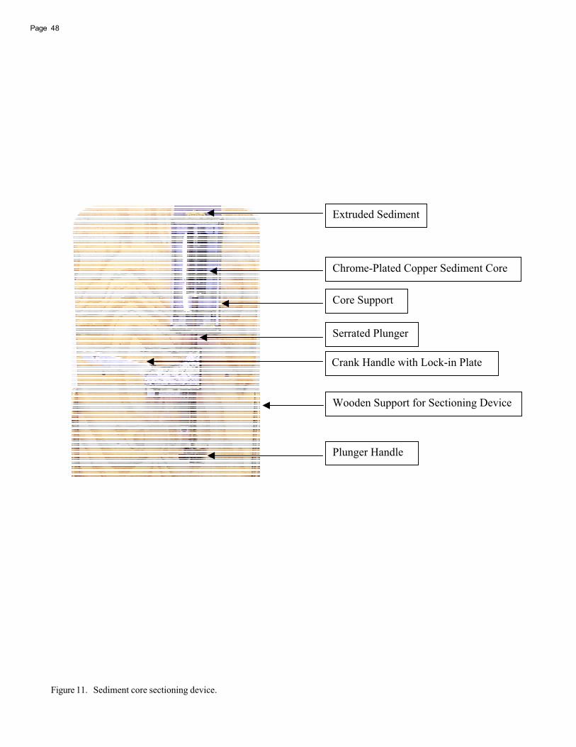
Chrome-Plated Copper Sediment Core

Extruded Sediment

Serrated Plunger

Wooden Support for Sectioning Device

Core Support

Plunger Handle

Crank Handle with Lock-in Plate

Page 48

Figure 11. Sediment core sectioning device.

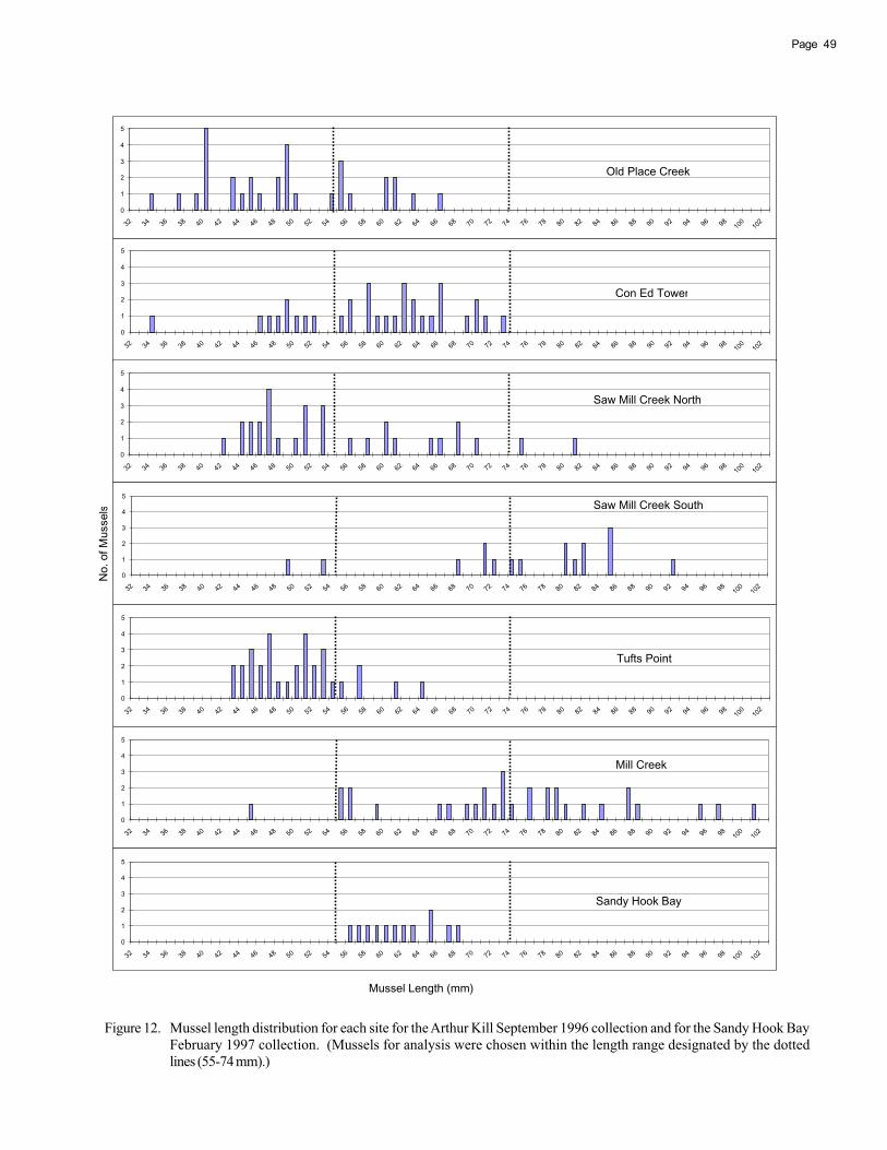
49Page

Figure 12. Mussel length distribution for each site for the Arthur Kill September 1996 collection and for the Sandy Hook BayFebruary 1997 collection. (Mussels for analysis were chosen within the length range designated by the dottedlines (55-74 mm).)

Mussel Length (mm)

0

1

2

3

4

5

32 34 36 38 40 42 44 46 48 50 52 54 56 58 60 62 64 66 68 70 72 74 76 78 80 82 84 86 88 90 92 94 96 98100 102

Con Ed Tower

0

1

2

3

4

5

32 34 36 38 40 42 44 46 48 50 52 54 56 58 60 62 64 66 68 70 72 74 76 78 80 82 84 86 88 90 92 94 96 98100 102

Old Place Creek

0

1

2

3

4

5

32 34 36 38 40 42 44 46 48 50 52 54 56 58 60 62 64 66 68 70 72 74 76 78 80 82 84 86 88 90 92 94 96 98100 102

Saw Mill Creek North

0

1

2

3

4

5

32 34 36 38 40 42 44 46 48 50 52 54 56 58 60 62 64 66 68 70 72 74 76 78 80 82 84 86 88 90 92 94 96 98100 102

Saw Mill Creek South

0

1

2

3

4

5

32 34 36 38 40 42 44 46 48 50 52 54 56 58 60 62 64 66 68 70 72 74 76 78 80 82 84 86 88 90 92 94 96 98100 102

Tufts Point

0

1

2

3

4

5

32 34 36 38 40 42 44 46 48 50 52 54 56 58 60 62 64 66 68 70 72 74 76 78 80 82 84 86 88 90 92 94 96 98100 102

Mill Creek

0

1

2

3

4

5

32 34 36 38 40 42 44 46 48 50 52 54 56 58 60 62 64 66 68 70 72 74 76 78 80 82 84 86 88 90 92 94 96 98100 102

Sandy Hook Bay

No.

of M

usse

ls

Page 50

Figure 13. Mussel length distribution for each site for the Arthur Kill May 1997 collection. (Mussels for analysis werechosen within the length range designated by the dotted lines (55-74 mm). No additional mussels were collectedat Sandy Hook Bay during May 1997.)

Mussel Length (mm)

0

1

2

3

4

5

32 34 36 38 40 42 44 46 48 50 52 54 56 58 60 62 64 66 68 70 72 74 76 78 80 82 84 86 88 90 92 94 96 98 100

Con Ed Tower

0

1

2

3

4

5

32 34 36 38 40 42 44 46 48 50 52 54 56 58 60 62 64 66 68 70 72 74 76 78 80 82 84 86 88 90 92 94 96 98 100

Old Place Creek

0

1

2

3

4

5

32 34 36 38 40 42 44 46 48 50 52 54 56 58 60 62 64 66 68 70 72 74 76 78 80 82 84 86 88 90 92 94 96 98 100

Saw Mill Creek North

0

1

2

3

4

5

32 34 36 38 40 42 44 46 48 50 52 54 56 58 60 62 64 66 68 70 72 74 76 78 80 82 84 86 88 90 92 94 96 98 100

Saw Mill Creek South

0

1

2

3

4

5

32 34 36 38 40 42 44 46 48 50 52 54 56 58 60 62 64 66 68 70 72 74 76 78 80 82 84 86 88 90 92 94 96 98 100

Tufts Point

0

1

2

3

4

5

32 34 36 38 40 42 44 46 48 50 52 54 56 58 60 62 64 66 68 70 72 74 76 78 80 82 84 86 88 90 92 94 96 98 100

Mill Creek

No.

of M

usse

ls

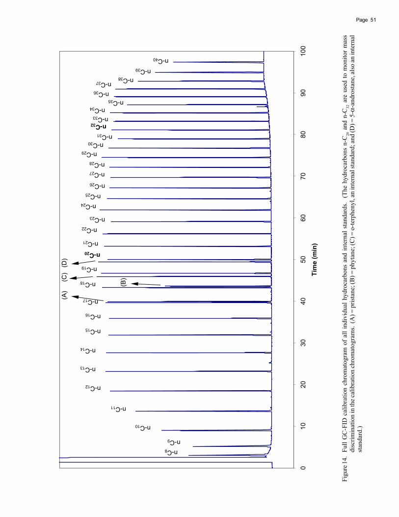
010

2030

4050

6070

8090

100

Tim

e (m

in)

n-C8

n-C9

n-C10

n-C11

n-C12

n-C13

n-C14

n-C15

n-C16

n-C17

n-C18

(A)

(B)

n-C19

n-C20

n-C22

n-C40

n-C24

n-C26

n-C28

n-C30

n-C32

n-C34

n-C36

n-C38

(D)

(C)

n-C21

n-C23

n-C25

n-C27

n-C29

n-C31

n-C33

n-C35

n-C37

n-C39

51Page

Figu

re 14

.Fu

ll G

C-F

ID c

alib

ratio

n ch

rom

atog

ram

of

all i

ndiv

idua

l hyd

roca

rbon

s an

d in

tern

al s

tand

ards

. (T

he h

ydro

carb

ons

n-C

20 a

nd n

-C32

are

use

d to

mon

itor

mas

sdi

scrim

inat

ion

in th

e cal

ibra

tion

chro

mat

ogra

ms.

(A) =

pris

tane

; (B

) = p

hyta

ne; (

C) =

o-te

rphe

nyl,

an in

tern

al st

anda

rd; a

nd (D

) = 5

-α-a

ndro

stan

e, al

so an

inte

rnal

stan

dard

.)

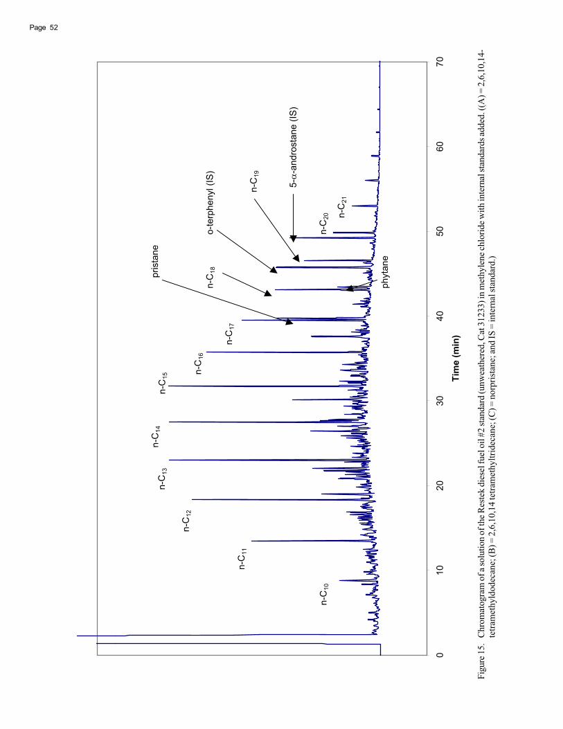
010

2030

4050

6070

Tim

e (m

in)

o-te

rphe

nyl (

IS)

5--a

ndro

stan

e (IS

)

n-C

19

n-C

20 n-C

21

n-C

12

n-C

13n-

C14

n-C

15

n-C

16

n-C

11

n-C

10

pris

tane

phyt

ane

n-C

17

n-C

18

Page 52

Figu

re 15

.C

hrom

atog

ram

of a

solu

tion

of th

e Res

tek

dies

el fu

el o

il #2

stan

dard

(unw

eath

ered

, Cat

312

33) i

n m

ethy

lene

chlo

ride w

ith in

tern

al st

anda

rds a

dded

. ((A

) = 2

,6,1

0,14

-te

tram

ethy

ldod

ecan

e; (B

) = 2

,6,1

0,14

tetra

met

hyltr

idec

ane;

(C) =

nor

pris

tane

; and

IS =

inte

rnal

stan

dard

.)

0 10 20 30 40 50 60 70

Time (in min.)

Restek Diesel Fuel #2 Standard

n-C20

n-C21n-C22

n-C19

n-C15

n-C17

n-C24n-C23

n-C18

n-C25

n-C16

n-C14

n-C11

n-C12

n-C13

n-C10

5- -Androstane (IS)

o-Terphenyl (IS)

Phytane

Pristane

CB

A

C - Norpristane

A - 2,6,10,14-Tetramethyldodecane

B - 2,6,10,14-Tetramethyltridecane

0 10 20 30 40 50 60 70

Spiked Sandy Hook Mussel Homogenate

n-C15

n-C17

n-C18

n-C16

n-C14

n-C11

n-C12

n-C13

n-C10

5- -Androstane (IS)o-Terphenyl(IS)

Area Sum-Hydrocarbon Peaks

0 10 20 30 40 50 60 70

Sandy Hook Mussel Homogenate Background

o-Terphenyl (IS)

5- -Androstane (IS)

Area Sum-Hydrocarbon Peaks

53Page

Figure 16. Chromatograms of Sandy Hook ribbed-mussel homogenate spiked with 1000 μg of Restek diesel fuel oil #2standard. (“Area Sum - Hydrocarbon Peaks” = sum of peak areas for n-C12, n-C13, n-C14, n-C15, n-C16, and n-C17only.)

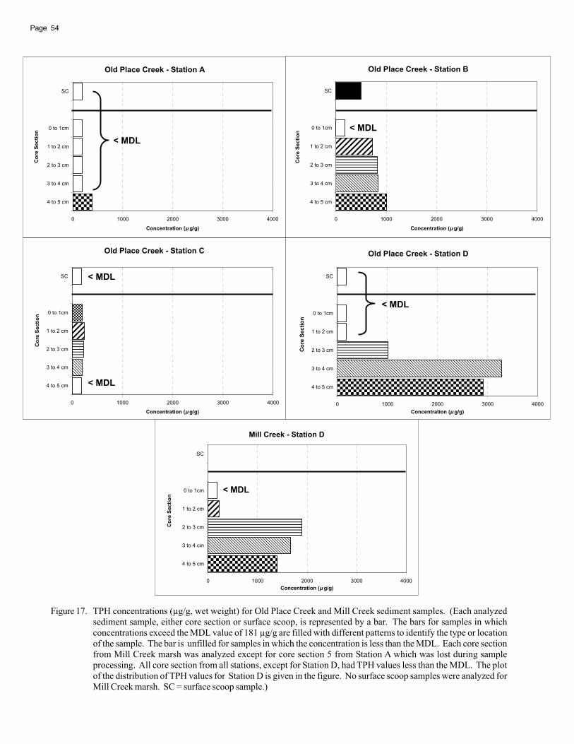
Old Place Creek - Station A

0 1000 2000 3000 4000

4 to 5 cm

3 to 4 cm

2 to 3 cm

1 to 2 cm

0 to 1cm

SC

Cor

e Se

ctio

n

Concentration (μ g/g)

< MDL

Old Place Creek - Station B

0 1000 2000 3000 4000

4 to 5 cm

3 to 4 cm

2 to 3 cm

1 to 2 cm

0 to 1cm

SC

Cor

e Se

ctio

n

Concentration (μ g/g)

< MDL

Old Place Creek - Station C

0 1000 2000 3000 4000

4 to 5 cm

3 to 4 cm

2 to 3 cm

1 to 2 cm

0 to 1cm

SC

Cor

e Se

ctio

n

Concentration (μ g/g)

< MDL

< MDL

Old Place Creek - Station D

0 1000 2000 3000 4000

4 to 5 cm

3 to 4 cm

2 to 3 cm

1 to 2 cm

0 to 1cm

SC

Cor

e Se

ctio

n

Concentration (μ g/g)

< MDL

Mill Creek - Station D

0 1000 2000 3000 4000

4 to 5 cm

3 to 4 cm

2 to 3 cm

1 to 2 cm

0 to 1cm

SC

Cor

e Se

ctio

n

Concentration (μ g/g)

< MDL

Page 54

Figure 17. TPH concentrations (μg/g, wet weight) for Old Place Creek and Mill Creek sediment samples. (Each analyzedsediment sample, either core section or surface scoop, is represented by a bar. The bars for samples in whichconcentrations exceed the MDL value of 181 μg/g are filled with different patterns to identify the type or locationof the sample. The bar is unfilled for samples in which the concentration is less than the MDL. Each core sectionfrom Mill Creek marsh was analyzed except for core section 5 from Station A which was lost during sampleprocessing. All core section from all stations, except for Station D, had TPH values less than the MDL. The plotof the distribution of TPH values for Station D is given in the figure. No surface scoop samples were analyzed forMill Creek marsh. SC = surface scoop sample.)

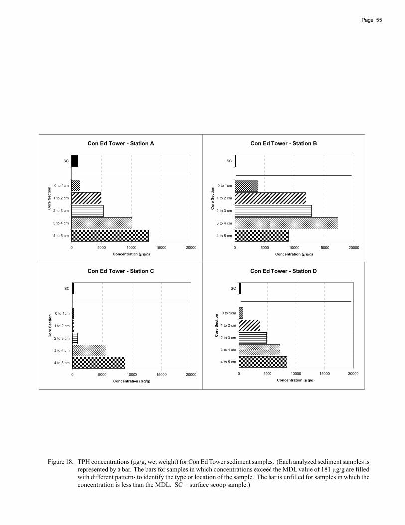
Con Ed Tower - Station A

0 5000 10000 15000 20000

4 to 5 cm

3 to 4 cm

2 to 3 cm

1 to 2 cm

0 to 1cm

SC

Cor

e Se

ctio

n

Concentration (μ g/g)

Con Ed Tower - Station B

0 5000 10000 15000 20000

4 to 5 cm

3 to 4 cm

2 to 3 cm

1 to 2 cm

0 to 1cm

SC

Cor

e Se

ctio

n

Concentration (μ g/g)

Con Ed Tower - Station C

0 5000 10000 15000 20000

4 to 5 cm

3 to 4 cm

2 to 3 cm

1 to 2 cm

0 to 1cm

SC

Cor

e Se

ctio

n

Concentration (μ g/g)

Con Ed Tower - Station D

0 5000 10000 15000 20000

4 to 5 cm

3 to 4 cm

2 to 3 cm

1 to 2 cm

0 to 1cm

SC

Cor

e Se

ctio

n

Concentration (μ g/g)

55Page

Figure 18. TPH concentrations (μg/g, wet weight) for Con Ed Tower sediment samples. (Each analyzed sediment samples isrepresented by a bar. The bars for samples in which concentrations exceed the MDL value of 181 μg/g are filledwith different patterns to identify the type or location of the sample. The bar is unfilled for samples in which theconcentration is less than the MDL. SC = surface scoop sample.)

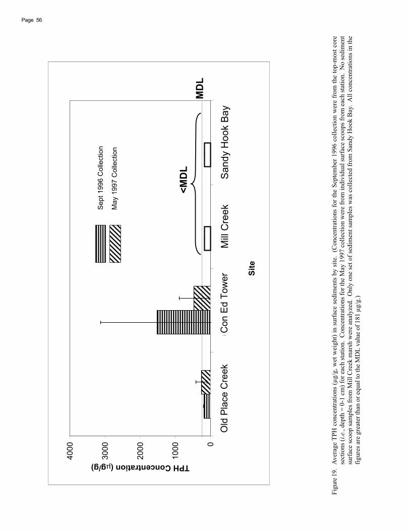
0

1000

2000

3000

4000

Old

Pla

ceC

on E

diso

nTo

wer

Mill

Cre

ekS

andy

Hoo

k B

ay

Site

TPH Concentration (g/g)

<MD

LM

DL

Sep

t 199

6 C

olle

ctio

n

May

199

7 C

olle

ctio

n

Old

Pla

ce C

reek

Con

Ed

Tow

er

Page 56

Figu

re 19

.Av

erag

e TP

H c

once

ntra

tions

(μg/

g, w

et w

eigh

t) in

sur

face

sed

imen

ts b

y si

te.

(Con

cent

ratio

ns fo

r the

Sep

tem

ber 1

996

colle

ctio

n w

ere

from

the

top-

mos

t cor

ese

ctio

ns (i

.e.,

dept

h =

0-1

cm) f

or e

ach

stat

ion.

Con

cent

ratio

ns fo

r the

May

199

7 co

llect

ion

wer

e fr

om in

divi

dual

surf

ace

scoo

ps fr

om e

ach

stat

ion.

No

sedi

men

tsu

rfac

e sc

oop

sam

ples

from

Mill

Cre

ek m

arsh

wer

e an

alyz

ed.

Onl

y on

e se

t of s

edim

ent s

ampl

es w

as c

olle

cted

from

San

dy H

ook

Bay

. A

ll co

ncen

tratio

ns in

the

figur

es ar

e gre

ater

than

or e

qual

to th

e MD

L va

lue o

f 181

μg/

g.)

050100

150

200

250

300

350

400

450

500

Old

Pla

ceC

on E

diso

n To

wer

Saw

Mill

Nor

thS

aw M

ill S

outh

Tufts

Poi

ntM

ill C

reek

San

dy H

ook

Bay

Site

s

Concentration

Sep

t 199

6 C

olle

ctio

n at

Arth

ur

Kill

May

199

7 C

olle

ctio

n at

Arth

ur

Kill

Col

lect

ion

at S

andy

Hoo

k B

ay

MD

L

Old

Pla

ce C

reek

Saw

Mill

Cre

ek S

outh

Saw

Mill

Cre

ek N

orth

57Page

Figu

re 20

.Av

erag

eTP

H c

once

ntra

tions

(μg/

g, w

et w

eigh

t) in

ribb

ed-m

usse

ls b

y si

te.

(One

set o

f rib

bed-

mus

sels

was

col

lect

ed a

t San

dy H

ook

Bay

bet

wee

n th

e co

llect

ion

date

s for

the t

wo

sets

ofA

rthur

Kill

sam

ples

. To

calc

ulat

e the

aver

age w

here

som

e mem

bers

had

val

ues l

ess t

han

the M

DL,

one

-hal

f of t

he M

DL

was

use

d. W

hen

the a

vera

ge v

alue

exce

eded

the M

DL,

the b

ars a

re fi

lled.

The

aver

age f

or th

e Saw

Mill

Cre

ek S

outh

Sep

tem

ber 1

996

colle

ctio

n w

as le

ss th

an th

e MD

L (5

3.6

μg/g

).Th

e va

lue

for t

he M

DL

was

use

d in

the

plot

, and

the

bar w

as n

ot fi

lled.

)

-500500

1500

2500

3500

4500

OP:

Sep

t 96

OP:

May

97

CET

: Sep

t 96

CET

: May

97

MC

: Sep

t 96

SH

Non

-Out

lier M

axN

on-O

utlie

r Min

75%

25%

Med

ian

Ext

rem

es

Page 58

Figu

re 21

.B

ox p

lot o

f the

TPH

conc

entra

tions

(μg/

g, w

et w

eigh

t) in

surfa

ce se

dim

ents

. (O

P =

Old

Pla

ce C

reek

; CET

= C

on E

d To

wer

; MC

= M

ill C

reek

; and

SH

= S

andy

Hoo

kBa

y.)

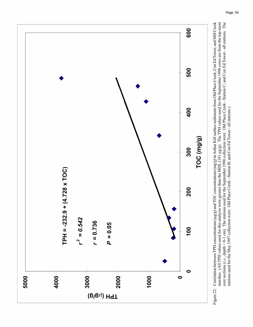
0

1000

2000

3000

4000

5000

010

020

030

040

050

060

0

TOC

(mg/

g)

TPH (g/g)

TPH

= -2

32.9

+ (4

.728

x T

OC

)

r2 =

0.5

42

r =

0.73

6

P =

0.0

5

59Page

Figu

re 2

2.Co

rrela

tion

betw

een T

PH co

ncen

tratio

ns (μ

g/g)

and T

OC

conc

entra

tions

(mg/

g) in

Arth

ur K

ill su

rface

sedi

men

ts fro

m O

ld P

lace

Cre

ek, C

on E

d Tow

er, a

nd M

ill C

reek

mar

shes

. (A

ll TP

H v

alue

s use

d fo

r thi

s ana

lysi

s wer

e gre

ater

than

the M

DL

(181

μg/

g).

The T

PH v

alue

s use

d fo

r the

Sep

tem

ber 1

996

core

s are

from

the t

op-m

ost

core

sect

ions

(i.e

., de

pth

= 0-

1 cm

). T

he st

atio

ns u

sed

for t

he S

epte

mbe

r 199

6 co

llect

ion

wer

e: O

ld P

lace

Cre

ek -

Stat

ion

C; a

nd C

on E

d To

wer

- al

l sta

tions

. The

stat

ions

use

d fo

r the

May

199

7 co

llect

ion

wer

e: O

ld P

lace

Cre

ek -

Stat

ion

B; a

nd C

on E

d To

wer

- al

l sta

tions

.)

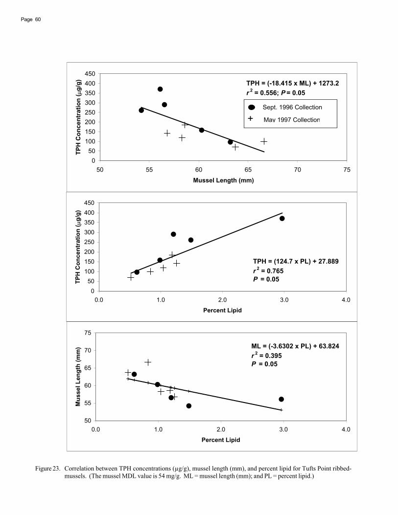
TPH = (-18.415 x ML) + 1273.2r 2 = 0.556; P = 0.05

050

100150200250300350400450

50 55 60 65 70 75

Mussel Length (mm)

TPH

Con

cent

ratio

n (

g/g)

Sept. 1996 Collection

+ May 1997 Collection

TPH = (124.7 x PL) + 27.889r 2 = 0.765P = 0.05

050

100150200250300350400450

0.0 1.0 2.0 3.0 4.0

Percent Lipid

TPH

Con

cent

ratio

n (

g/g)

ML = (-3.6302 x PL) + 63.824r 2 = 0.395P = 0.05

50

55

60

65

70

75

0.0 1.0 2.0 3.0 4.0

Percent Lipid

Mus

sel L

engt

h (m

m)

Page 60

Figure 23. Correlation between TPH concentrations (μg/g), mussel length (mm), and percent lipid for Tufts Point ribbed-mussels. (The mussel MDL value is 54 mg/g. ML = mussel length (mm); and PL = percent lipid.)

Saw Mill Creek South Marsh

ML = (-17.263 x PL) + 75.661r 2 = 0.619r = 0.787P = 0.05

50

55

60

65

70

75

0.0 0.2 0.4 0.6 0.8 1.0 1.2

Percent Lipid

Mus

sel L

engt

h ( m

m)

Mill Creek Marsh

ML = (10.421 x PL) + 51.332r 2 = 0.500r = 0.707P = 0.05

50

55

60

65

70

75

0.0 0.2 0.4 0.6 0.8 1.0 1.2 1.4 1.6 1.8

Percent Lipid

Mus

sel L

engt

h (m

m)

Saw Mill Creek North Marsh

TPH = (170.16 x PL) - 63.84r 2 = 0.760r = 0.872P = 0.05

0

50

100

150

200

250

300

0.0 0.5 1.0 1.5 2.0 2.5

Percent Lipid

TPH

Con

cent

ratio

n (

g/g)

Sept 1996 Collection

+ May 1997 Collection

61Page

Figure 24. Correlation between TPH concentrations (μg/g) and percent lipid in Saw Mill Creek North ribbed-mussels, corre-lation between mussel length (mm) and percent lipid in Saw Mill Creek South ribbed-mussels, and correlationbetween mussel length (mm) and percent lipid in Mill Creek ribbed-mussels. (The mussel MDL value is 54 mg/g.ML = mussel length (mm); and PL = percent lipid.)

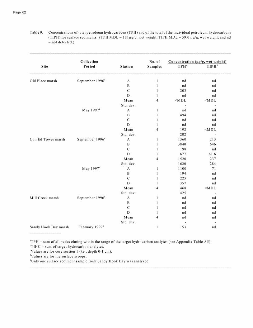
Table 9. Concentrations of total petroleum hydrocarbons (TPH) and of the total of the individual petroleum hydrocarbons

(TIPH) for surface sediments. (TPH MDL = 181μg/g, wet weight; TIPH MDL = 59.0 μg/g, wet weight; and nd

= not detected.)

_________________________________________________________________________________________________

Collection No. of Concentration (μg/g, wet weight)

Site Period Station Samples TPH TIPHa b

_________________________________________________________________________________________________

Old Place marsh September 1996 A 1 nd ndc

B 1 nd nd

C 1 203 nd

D 1 nd nd

Mean 4 <MDL <MDL

Std. dev. - -

May 1997 A 1 nd ndd

B 1 494 nd

C 1 nd nd

D 1 nd nd

Mean 4 192 <MDL

Std. dev. 202 -

Con Ed Tower marsh September 1996 A 1 1360 213c

B 1 3840 646

C 1 198 nd

D 1 677 61.6

Mean 4 1520 237

Std. dev. 1620 284

May 1997 A 1 1100 71d

B 1 194 nd

C 1 225 nd

D 1 357 nd

Mean 4 468 <MDL

Std. dev. 425 -

Mill Creek marsh September 1996 A 1 nd ndc

B 1 nd nd

C 1 nd nd

D 1 nd nd

Mean 4 nd nd

Std. dev. - -

Sandy Hook Bay marsh February 1997 1 153 nde

_______________

TPH = sum of all peaks eluting within the range of the target hydrocarbon analytes (see Appendix Table A5).a

TIHC = sum of target hydrocarbon analytes.b

Values are for core section 1 (i.e., depth 0-1 cm).c

Values are for the surface scoops.d

Only one surface sediment sample from Sandy Hook Bay was analyzed.e

_________________________________________________________________________________________________

Page 62

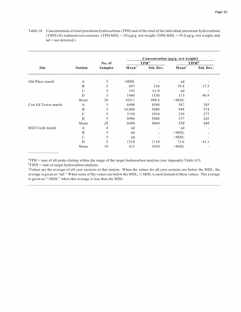
Table 10. Concentrations of total petroleum hydrocarbons (TPH) and of the total of the individual petroleum hydrocarbons

(TIPH) for sediment core sections. (TPH MDL = 181μg/g, wet weight; TIPH MDL = 59.0 μg/g, wet weight; and

nd = not detected.)

_________________________________________________________________________________________________

Concentration (μg/g, wet weight)

No. of TPH TIPHa b

Site Station Samples Mean Std. Dev. Mean Std. Dev.c c

_________________________________________________________________________________________________

Old Place marsh A 5 <MDL - nd -

B 5 697 354 59.4 17.3

C 5 193 61.0 nd -

D 5 1480 1530 115 96.9

Mean 20 629.1 908.4 <MDL -

Con Ed Tower marsh A 5 6900 4560 587 285

B 5 10,900 5040 998 574

C 5 3150 3910 239 277

D 5 4980 3080 377 245

Mean 20 6490 4860 550 449

Mill Creek marsh A 4 nd - nd -

B 5 nd - <MDL -

C 5 nd - <MDL -

D 5 1310 1110 73.6 41.1

Mean 19 413 1030 <MDL -

_______________

TPH = sum of all peaks eluting within the range of the target hydrocarbon analytes (see Appendix Table A5).a

TIPH = sum of target hydrocarbon analytes.b

Values are the average of all core sections at that station. When the values for all core sections are below the MDL, thec

average is given as “nd.” When some of the values are below the MDL, ½ MDL is used instead of these values. The average

is given as “<MDL” when this average is less than the MDL.

_________________________________________________________________________________________________

63Page

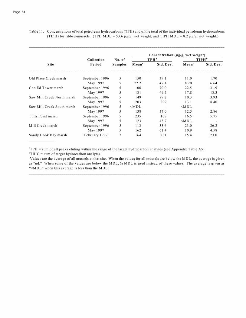
Table 11. Concentrations of total petroleum hydrocarbons (TPH) and of the total of the individual petroleum hydrocarbons

(TIPH) for ribbed-mussels. (TPH MDL = 53.6 μg/g, wet weight; and TIPH MDL = 8.2 μg/g, wet weight.)

_________________________________________________________________________________________________

Concentration (μg/g, wet weight)

Collection No. of TPH TIPHa b

Site Period Samples Mean Std. Dev. Mean Std. Dev.c c

_________________________________________________________________________________________________

Old Place Creek marsh September 1996 5 150 39.1 11.0 1.70

May 1997 5 72.2 47.1 8.20 6.64

Con Ed Tower marsh September 1996 5 106 70.0 22.5 31.9

May 1997 5 181 69.5 17.8 18.3

Saw Mill Creek North marsh September 1996 5 149 87.2 10.3 3.93

May 1997 5 203 209 13.1 8.40

Saw Mill Creek South marsh September 1996 5 <MDL - <MDL -

May 1997 5 138 37.0 12.5 2.86

Tufts Point marsh September 1996 5 235 108 16.5 5.75

May 1997 5 123 43.7 <MDL -

Mill Creek marsh September 1996 5 113 33.6 23.0 26.2

May 1997 5 162 61.4 10.9 4.58

Sandy Hook Bay marsh February 1997 7 164 281 15.4 23.0

TPH = sum of all peaks eluting within the range of the target hydrocarbon analytes (see Appendix Table A5).a

TIHC = sum of target hydrocarbon analytes.b

Values are the average of all mussels at that site. When the values for all mussels are below the MDL, the average is givenc

as “nd.” When some of the values are below the MDL, ½ MDL is used instead of these values. The average is given as

“<MDL” when this average is less than the MDL.

_________________________________________________________________________________________________

Page 64

65Page

IV. SEDIMENT BIOGEOCHEMISTRY

Vincent G. Guida14, 15 and Andrew F. J. Draxler14, 16

Postal Address: 14National Marine Fisheries Serv., 74 Magruder Rd., Highlands,NJ 07732

E-Mail Addresses: 15Vincent.Guida@noaa.gov; 16Andrew.Draxler@noaa.gov

The aforementioned characteristics are those of estab-lished, functioning wetland soils. The re-establishment ofproductive stands of S. alterniflora has clearly been suc-cessful in the replanted salt marshes of the Arthur Kill(Bergen et al. 2000). We have sought to determine if the re-establishment of normal wetland soil characteristics hasbeen as successful. Indeed, we seek to understand to whatextent oiling and other urban influences have affected theseunseen, but vital biogeochemical features of the Arthur Killsalt marshes.

Previous studies found that created wetlands had lowerOC and nitrogen content, but higher redox potential values(measured as Eh) and higher manganese and iron content,than natural wetlands (Craft et al. 1991; Zedler 1993). Otherstudies have shown that sediment organic content appearsto develop slowly in newly created salt marshes, and maytake years to reach natural levels (LaSalle et al. 1991; Moyand Levin 1991; Minello and Zimmerman 1992). Likewise,development of saltmarsh nitrogen cycling rates can re-quire years (Thompson et al. 1995). These differences be-tween newly created and established wetlands are relatedto the low organic matter content of soils used for de novowetland creation as compared with that of natural marshsoil. Such findings suggest that marshes planted onnonwetland soils cannot immediately duplicate the bio-geochemical functions of older, natural systems.

Unlike wetlands that have been “created” though, theArthur Kill marshes such as the one at Old Place Creek havebeen replanted on old wetland soils, although ones whichhave been highly altered in this urban environment. Priorto replanting, those sites were denuded due to the oil spill,and were barren for a few years until replanted. By compar-ing these replanted wetlands with the denuded areas thatwere not replanted and with areas that were not denuded,we hoped to investigate what effect these varied histories mayhave had on the organic matter essential for soil function.

The abundance of soluble inorganic sulfide, primarilyin the forms of the dissolved hydrosulfide ion (HS-) andhydrogen sulfide (H2S), is of particular interest because it isan indicator of microbial activity and recent redox history,and because it has a strong influence on primary produc-tion. Soluble sulfide is a product of a bacterial respiratorypathway that utilizes the abundant sulfate ion (SO4

-2) insaline interstitial water as a source of oxidizing power whereother oxidants (including O2 and NO3

-) have been depleted.Sulfate reduction is a major form of respiration in salt marshes(Howarth and Giblin 1983), and the sulfide produced is

INTRODUCTION

Knowledge of soil biogeochemistry in salt marshes isessential to an understanding of the role of these wetlandsin promoting fisheries. Biogeochemistry is the chemistrythat mediates interactions among atmosphere, water, miner-als, microbiota, and higher organisms in the environment.It is characterized by both linear and cyclic transformationsof materials, yielding deposits of end products for somematerials, a dynamic steady state for other materials, andthe generation of metabolic energy that sustains the struc-ture of the ecosystem.

Organic wetland soils (i.e., hydric histosols) such asthose in salt marshes have a great capacity for transforma-tions of forms of carbon, nitrogen, phosphorus, sulfur, andtransition metals. These transformations are essential tothe productivity and structure of salt marshes, and therebyto the functioning of these marshes as critical fisheries habi-tat (Boesch and Turner 1984). The same transformationsare also critical as exporters of production to adjacent wa-ters (Haines 1979).

Saturation of wetland soils with water impedes the dif-fusion of gaseous atmospheric oxygen into such soils.Water, through which oxygen diffuses slowly, fills the inter-stices between solid particles that would otherwise be filledwith gas, through which oxygen diffuses rapidly. At thesame time, water saturation facilitates the diffusion of non-gaseous water-soluble materials. The result is a sharp de-cline in the reducing-oxidizing (i.e., redox) potential withdepth that is characteristic of wetland soils, and one thatleads to other characteristics typical of wetland soils (Mitschand Gosselink 1986).

Some of these other characteristics include anoxia whichallows the net accumulation of organic matter from deadplant parts that cannot be converted entirely to carbon di-oxide and water without an oxidant, thus allowing the de-velopment and maintenance of the characteristically highorganic matter content of the histosol. Another character-istic resulting from the abundant organic matter and redoxpotential gradient is the variety of microenvironments fa-voring an array of microbiota with extremely diverse meta-bolic capabilities. These capabilities include the cyclic re-dox transformations of nitrogen, sulfur, iron, and manga-nese that are essential to maintaining primary production,and a variety of organic decay mechanisms that allow trans-fer of energy from refractory lignocellulose plant remainsinto the trophic web (Howes et al. 1984; Newell 1993).

Page 66

known to inhibit root uptake of nitrogen in S. alternifloraand other wetland plants (Bradley and Morris 1990a; Kochet al. 1990). In the case of S. alterniflora, sulfide inhibitionof nitrogen uptake, along with salinity inhibition, are poten-tially important sources of productivity limitation sincegrowth of this grass appears to be nitrogen-limited in mostGulf and Atlantic Coast marshes (Bradley and Morris 1992).

While measurement of sulfide deals with a narrow setof redox species, measurement of soil Eh integrates the in-fluence of many such chemical species (e.g., O2 , Fe+3, Fe+2,Mn+4, Mn+2, NH4

+, NO3-, H2S, HS-, CH4, H2, etc.). Typical

depth profiles for Eh in saltmarsh soils have high positivevalues at the surface, indicating the penetration of hydro-spheric and atmospheric O2. This surface layer is underlainby a rapid decline in values within the first few centimeters,indicating exhaustion of O2. Below this rapid decline, thereis a continuous slow decline in Eh toward values character-izing sulfide presence, perhaps underlain by still lower val-ues indicating exhaustion of sulfate substrate and support-ing only fermentative metabolism (Howes et al. 1981).

Aside from depth in the soil, Eh values are influencedby the presence or absence of vegetation, the type of veg-etation, and the seasonal state (i.e., dormancy vs. activegrowth) of vegetation (de la Cruz et al. 1989). During thegrowing season, S. alterniflora oxidizes marsh soil (in-creases Eh) by conducting oxygen downward into its rootsand by diffusion to the adjacent soil root zone via special-ized aerenchyma tissues. In addition, the grass lowers soilwater saturation levels by transferring interstitial water tothe atmosphere via evapotranspiration (Howes et al. 1981).Such processes are not active during the dormant season(fall-winter) or where grass has been intentionally burnt orclipped or has died back of other causes; such factors re-sult in lower Eh values that appear to inhibit recolonizationin dieback areas where rhizosphere oxidation cannot be re-established simply by reactivation of existing root and rhi-zome systems (Bertness 1991). On the other hand, low Ehvalues can also result in the release into interstitial water ofdissolved inorganic nutrients essential to plant growth(DeLaune et al. 1981).

The presence of living S. alterniflora, with its seasonaloxidizing influence (i.e., raising Eh values) and release ofsoluble organic materials into soils, has important conse-quences for the biogeochemistry of salt marshes. In addi-tion to raising the Eh, the microzones around cordgrassroots: 1) exhibit lower pH; 2) accumulate and immobilizeforms of such potentially toxic metals as copper, zinc, andlead, presumably due to the tight binding of such metals toabundant organic ligands (Caçador et al. 1996); 3) oxidizesulfide (Howes et al. 1981); 4) mobilize iron (Kostka andLuther 1995); and 5) facilitate the redox cycling of iron viaorganic ligand complexes (Luther et al. 1992). These alter-ations in cordgrass root microzones form a positive feed-back on the growth of cordgrass, for which iron is essentialand sulfide and excess heavy metals are toxic. Such bio-geochemical functions are presumably lost when cordgrassroots die, resulting in greater mobility of heavy metals, higher

sulfide levels, and immobilization of iron, making soil lesssuitable for re-establishment and growth of S. alterniflora.

Finally, there is the effect of residual petroleum con-tamination on biogeochemical functions in Arthur Killmarshes. Early research with crude oil suggested that thissubstance may not be very toxic to such important micro-bial processes as the fixation of nitrogen (Thomson andWebb 1984), the reduction of nitrate, manganese, iron, andsulfate, and the production of methane and ammonia(DeLaune et al. 1979). However, subsequent work withspecific oil components has shown that naphthalene caninhibit sulfate reduction in saltmarsh sediments while in-creasing methanogenesis (Keine and Capone 1984). In-deed, there is evidence that fuel oil can increase detritaldecay rates (Hershner and Lake 1980), and that low levelsof a light hydrocarbon mixture can stimulate CO2 produc-tion, methanogenesis, nitrogen fixation, and denitrificationin saltmarsh soils (Li et al. 1990).

Because of the key roles played by soil organic matter,sulfide, and redox potential in controlling saltmarsh struc-ture and productivity, we have chosen to measure total andlabile (i.e., readily degraded by aerobic microbiota) organicmatter in soil, and soluble sulfide and Eh values in intersti-tial water, as means of characterizing and assessing thecomparative biogeochemical condition of Arthur Killmarshes and the possible efficacy of the replanting efforts.

METHODS AND MATERIALS

At each of the six sites, four stations were selected at0.2 m above mid-tide. The separation between replicatestations at a site ranged between 2 and 20 m (see descrip-tion of the sampling transect in Chapter II, “Trace MetalContaminants in Sediments and Ribbed-Mussels”). In or-der to take into account seasonal variations, sampling re-gimes were performed during two intervals: September-October 1996 representing fall, and May 1997 representingspring.

Redox Potential

Duplicate vertical profiles of redox potential (measuredas Eh) were taken in situ within 10 cm of each other at eachstation using a Fisher Scientific Model 640 portable pH/millivolt meter. The instrument was calibrated to within 1mV at 10, 100, and 1000 mV using a Cole-Parmer pH-mVcalibrator (#5657-10). A platinum electrode (Thomas Scien-tific #4096-D20) with a band of platinum (6-mm dia. × 4-mmheight) was used as the sample electrode. The referenceelectrode was a Fisher Scientific (#13-639-62) sleeve-junc-tion calomel electrode. This system was calibrated usingthree K3Fe(CN)6-K4Fe(CN)6 solutions of differing redox po-tentials (ZoBell 1946; Orion Research, Inc. 1983).

Depth in the sediment was measured to the center ofthe band except for the “zero” reading which was made with

67Page

the band just immersed in the sediment. Before each pro-file, the electrode system was equilibrated in water collectedin the Arthur Kill adjacent to the site. In the first profile,measurements were made in overlying surface water at 1 cmabove the soil surface, at the soil surface (0), 0.5 cm belowthe surface, and 1-5 cm below the surface at 1-cm intervals,soil penetrability permitting. In the second profile, mea-surements were made 1-10 cm below the soil surface at 1-cmintervals, soil penetrability permitting. Readings at eachdepth interval were accepted when the rate of change was<1 mV in 10 s.

Soluble Sulfide

Samples for porewater sulfide determination were ob-tained with the use of de-ionized water (DIW) equilibrationdevices, or “peepers” (Hesslein 1976; C. Wigand, U.S. En-vironmental Protection Agency, 27 Tarzwell Dr.,Narragansett, RI, pers. comm.; Figure 25). These devicesobtained time-integrated, particulate-free samples of waterwith the same dissolved chemical composition as intersti-tial water by allowing an extended period of equilibrationsbetween water outside the peeper and DIW inside the peeperacross membranes with molecule-sized pores. Each peeperconsisted of a body and two face plates (one on each side)of high-density polyethylene (HPDE) held together withstainless steel screws and washers. Sandwiched betweenthe body and face plates and enclosing five pairs of cylin-drical equilibration chambers (each 2.54-cm dia. × 1.9-cmdepth, with a capacity of 9.7 ml) were two cellulose dialysismembranes (Spectra/Por1) made from regenerated celluloseand having a molecular weight cutoff of 6000-8000 Daltons.

In order to avoid contamination of subsurface soil andporewater with molecular oxygen from the peepers, theHPDE peeper parts were soaked for 25 days in DIW whichhad been continuously sparged with N2 gas in order toremove adsorbed O2 prior to assembly. To minimize O2 ab-sorption before insertion in marsh soil, peeper chamberswere filled with N2-sparged DIW, and the assembled peep-ers were wrapped in polyvinylidine chloride film and weretransported in N2-sparged water. Peepers used in 1996 hada single set of vertical chambers, while those used in 1997had two sets, as depicted in Figure 25. As each chamberspanned 2.54 cm in the vertical dimension, samples from thefive pairs of samples represent conditions from the follow-ing height/depth ranges (+ is above the soil surface and - isbelow): 1) +3.2 to +0.6 cm (mean = +1.9 cm); 2) -0.6 to -3.2 cm(mean = -1.9 cm); 3) -4.4 to -7.0 cm (mean = -5.7 cm); 4) -8.3 to-10.8 cm (mean = -9.5 cm); and 5) -13.3 to -15.9 cm (mean =-14.6 cm).

Each peeper was driven into the soil with a rubber mal-let at one (1996) or two (1997) randomly chosen stationsfrom among the four stations at each site so that four setsof chambers were below the surface of the soil and oneabove (Figure 25). The peepers were left undisturbed toequilibrate with the porewater for 13-14 days. Upon re-

trieval, the cellulose membranes covering each chamber werepunctured with a Teflon needle (reused after flushing withsurface seawater), and samples were withdrawn from thechamber with disposable syringes and transferred to 1.5-mlpolypropylene centrifuge tubes for immediate addition ofcolorimetric reagents and dilution water (i.e., N2-sparged,filtered seawater). Sample dilution by 10- or 100-fold wasnecessary to overcome the limitations of the analyticalmethod.

Analysis was performed by a micromethod derived fromthe method of Strickland and Parsons (1972), with reagentscalibrated against iodometric titration, and standardizationperformed using serial dilutions of sulfide-enriched, N2-sparged seawater. Optical absorbance of the samples wasdetermined with a Perkin Elmer Lambda 3B spectrophotom-eter within 4 hr of collection. Tests of this microprocedurehave shown a 2.07±3.04% (i.e., mean ± standard deviation;n = 8) decrease in absorbance of samples after 7 hr of reac-tion time. Total procedural error for the method was ±10%(n = 26) for sulfide values up to 900 μM. Values between900 and 3000 μM were ±30%. Values beyond 3000 couldnot be estimated by our method, and were recorded as“>3000 μM.”

Total Organic Carbon

Sediment samples for the determination of TOC weremanually collected in 28-mm (internal diameter) butyratecores, one core per station, to an average depth of 10 cm.Care was taken to prevent disturbance of the sediment sur-face layer by maintaining the cores upright on ice for thereturn to the laboratory, where they were frozen at -20°Cuntil processed. Frozen sediment cores were transferred toa 4°C cold room and defrosted. The cored sediment wasextruded; the surface layer (to a depth of 1 cm) was col-lected in individual precleaned glass containers. Due to thevegetated nature of the collection sites, sectioning of thesediment was accomplished with a serrated stainless steelblade. Sectioned sediments were dried overnight at 50°C.All large carbonaceous fragments (>1 mm) were removed;samples were then homogenized with a glass rod. A 100-mgsubsample was transferred into an acid-cleaned, uncappedscintillation vial. The acidification technique of Yamamuroand Kayanne (1995) was employed to remove carbonate,while avoiding the dissolution of acid-soluble organic ma-terial.

Aliquots, ranging from 10 to 50 mg, were taken from theacidified samples, placed into tin combustion cups, andsealed in preparation for organic carbon and nitrogen analy-ses by flash combustion in oxygen at 1020°C on a CarloErba 1108 elemental analyzer equipped with a 120-positionautosampler. Combustion products pass over a catalystand then over copper to remove excess oxygen and to re-duce the nitrogen oxides to elemental nitrogen. Upon sepa-ration by gas chromatography, the CO2 and N2 eluent peaksare integrated and reported as organic carbon and nitrogen.

Page 68

Instrument calibration was maintained by performing a se-ries of linear regressions using an acetanilide standard.These standard and additional TOC SRMs (e.g., PACS-1)were placed into the sample rotation for further verificationof optimal operation.

Labile Carbon

The 0.1-cm3 sediment surface samples for labile carbon(LC) analysis were obtained by coring marsh sediments usingdisposable 10-ml plastic syringes with the tapered end cutoff. These cores included the upper 1 cm of the soil column.Duplicate samples were taken at each of two randomly cho-sen stations at each site during May 1997.

The LC content of these samples was estimated viameasurement of dissolved oxygen consumption by themicrobiota during a 13-day incubation of the sample in a300-ml BOD (biological oxygen demand) bottle filled withnatural seawater and maintained at 20°C (Draxler 1995).Sediment oxygen consumption was compared with oxygenconsumption by D-glucose under the same conditions.Therefore, sediment LC, hereafter reported as “μM-C/cm3,”signifies micromoles of glucose carbon equivalents per cu-bic centimeter of sediment.

Data Analysis

Statistical analyses of data were performed with the aidof Jandel Scientific SigmaStat 2.0. Procedures included theuse of Kruskal-Wallis, one-way ANOVA and the Mann-Whitney rank sum test for site-by-site comparison of redoxpotential, sulfide concentrations, and TOC content of soil,with the use of Tukey, Dunn’s, or Student-Newman-Keulspairwise tests, as appropriate, and of Student’s t-tests, forseasonal comparison of redox potential.

RESULTS

Redox Potential

A total of 965 measurements of Eh were made for thepurpose of creating duplicate depth profiles for redox po-tential in soil at four stations (designated A through D) ateach of the six sites in each of two seasons: fall 1996 andspring 1997 (Figures 26-28). Depths in the soil in these andall subsequent presentations are indicated in terms of nega-tive (-) elevations, with a zero value denoting the soil sur-face. Most, though not all, sites demonstrated the classicdeclining gradient in Eh with depth, described in the intro-duction to this chapter. The highest values were generallyat the surface. In most cases, a zone of rapid decline ofredox potential was within a depth of 2 cm, with more slowlydeclining values between -2 and -5 cm, then consistentlylow values below -5 cm.

Values of Eh for surface water collected adjacent to thesites were +268±37 mV (n = 47) during fall 1996, and +314±23mV (n = 46) during spring 1997 (Figures 26-28). Since the Ehrange of oxygenated pure water is above +350 mV, theselow values suggest poor quality in water overlying the marshduring high tide (i.e., little dissolved oxygen and/or an abun-dance of reductants such as organic matter).

Beneath the soil surface, some profiles within each sta-tion diverged from the classic pattern, yielding both ex-traordinarily low and extraordinarily high Eh values at depth(e.g., Figure 26A). While replanted sites appeared moreprone to high subsurface values (Figure 26), this phenom-enon was not uniformly demonstrated at all stations nor inall seasons within that treatment group, nor was it exclu-sively present there (Figures 27 and 28). Of the 40 highestvalues (+374 to +478 mV), 26 were taken at Old Place Creek- Station A during both fall and spring, and 11 from Saw MillCreek North - Station B in spring, making these the stationswith the most oxic sediments. Paradoxically, Old Place Creek(a replanted site) was also the site where the lowest (i.e.,most reduced) values of the study were recorded. Of the 21lowest values (>-251 mV), 16 came from Old Place Creek -Stations B, C, and D (replanted), making the deeper layersat these stations the most anoxic sediments of the study --a sharp contrast to the highly oxic character of sediments atOld Place Creek - Station A. Extremely low values wereevident at the reference sites (e.g., Figure 27A) as well.

While Eh declined with depth in the soil at most sta-tions, it increased with depth in a few profiles, includingthose for Old Place Creek - Station A (replanted), Saw MillCreek North - Station B (replanted), and Tufts Point - Sta-tion C (reference) in both fall and spring, and for Con EdTower - Stations A and C (unplanted) in spring only. Otherstations at those sites did not exhibit this pattern.

Unequal variances and deviations from normality pre-vented the use of parametric, three-way ANOVA of Eh datato detect significant differences by depth, season, restora-tion status, and station. Therefore, a separate nonparamet-ric test (i.e., the Kruskal-Wallis, one-way, ANOVA-on-rankstest) for depth, restoration status, and station, and another(i.e., the Mann-Whitney rank sum test) for season, wereemployed to test the significance of each of these factors.There was a significant difference associated with depth (P<0.001), and indeed, a significant linear correlation with thatfactor (r2 = 0.433, P <0.01). There were also significantdifferences by season, by treatment, and by station (all P<0.001). Spring Eh values were significantly higher than fallvalues. Dunn’s pairwise comparison test showed signifi-cant differences (P <0.05) between replanted and unplantedsites, and between replanted and reference sites; replantedmarshes had significantly higher redox potentials thanunplanted or reference marshes.

While the last finding suggests an effect of replantingstatus upon redox potentials, that pattern was not borneout by examination of Eh values by station. Dunn’s pairwisecomparison test demonstrated that high redox values forreplanted marshes were driven largely by exceptionally high

69Page

values from Old Place Creek. Despite some very low val-ues, Old Place Creek (replanted) had significantly highermedian redox potential than Mill Creek (reference), Con EdTower (unplanted), and Saw Mill Creek South (unplanted)sites (all P <0.05), while redox potential values from SawMill Creek North, the other replanted site, were only signifi-cantly greater than Mill Creek (reference) values (P <0.05).The only other significant comparison was between thetwo marshes in the reference treatment group, Tufts Pointand Mill Creek; Tufts Point had the higher values. Site wasmore influential than treatment.

The possible effect of replanting on patterns of sea-sonal shifts in redox potential (i.e., treatment × seasonaleffects) was also investigated. Seasonal changes in redoxvalues from fall to spring included cases of significant in-creases, significant decreases, and no significant change.Statistical comparison of Eh data across seasons in the faceof strong depth gradients was accomplished by performingStudent’s t-tests on mean data for the three depth zones(i.e., 0 to -2 cm, -3 to -5 cm, and below -5 cm) suggested bythe zonation patterns mentioned previously. The Eh valuesin 24 of the 72 site-depth zone combinations (33%) weresignificantly greater (more oxidized) in spring 1997 than infall 1996 (P <0.05). This phenomenon occurred at all depthsand at sites under all treatment regimes, including Con EdTower (unplanted), but not at all stations. Eight combina-tions (11%) had more oxidized conditions in the fall, includ-ing Old Place Creek (replanted) - Stations A and B , Con EdTower (unplanted) - Station C, and Saw Mill Creek South(unplanted) - Stations A and C. In terms of magnitude ofsignificant changes, increases also predominated over de-creases. Seasonal changes in redox potential were signifi-cantly larger where they increased (|ΔEh| = 243±148 mV)from fall to spring than where they decreased (|ΔEh| = 79±51mV) during that interval (P = 0.005). However, with thelargest number of station-depth zone combinations (32 ofthe 72, or 44%), no significant seasonal change in redoxpotential was found.

The stations with the most consistently reducing con-ditions between -3 and -10 cm despite the change of sea-sons were Saw Mill Creek South (unplanted) - Stations Aand B and Mill Creek (reference) - Stations B and C. Valuesfor soil measurements organized by depth zone, and theresults of seasonal statistical comparisons, are summarizedby station in Appendix Tables F1-F3. As with EH values andprofile shapes, seasonal redox changes did not sort intorecognizable patterns by replanting status. Rather, pat-terns in seasonal change or lack thereof appear to be sta-tion specific.

Soluble Sulfide

Soluble sulfide was measured in 120 “peeper” watersamples. As with the related Eh measurements, interstitialsulfide concentrations demonstrated distinct and fairly con-sistent patterns with respect to depth and season. Sulfide

increased with depth (P <0.05) and was more abundant infall 1996 than in spring 1997 at four of the six sites (Figures29-31) The exceptions were Con Ed Tower (unplanted) andTufts Point (reference).

At all stations within all sites, soluble sulfide concen-trations above the soil surface were <2 μM, and were <80μM within 3 cm of the sediment interface. With these dataremoved, site-to-site comparisons of sulfide showed sig-nificant differences (P <0.05), but treatment-to-treatmentcomparisons did not (i.e., Kruskal-Wallis, one-way, ANOVA-on-ranks test). Below the 5-cm depth in fall, Old Place Creek- Station C (replanted) had concentrations exceeding theanalytical limit of the analysis employed (>3000 μM). Else-where, sulfide concentration approached this level onlydeeper than 14 cm in fall at Mill Creek - Station C (reference;2700 μM) and at Saw Mill Creek South - Station D (unplanted;2650 μM). In spring, values at Old Place Creek - Station Afor all depths were <2 μM, while Old Place Creek - Station Bcontained 1250 μM below 14 cm in depth. Values at SawMill Creek North - Station C (also replanted) never exceeded200 μM in fall, or 100 μM in spring. At the Con Ed Tower(unplanted) and especially Tufts Point (reference) sites, theconcentration pattern seen elsewhere of high fall and lowspring values was reversed. The most similar pairs of pat-terns did not share common replanting status: Saw MillCreek South (unplanted) - Mill Creek (reference) (Figures30B and 31B), and Con Ed Tower (unplanted) - Saw MillCreek North (replanted) (Figures 30A and 29B).

Total Organic Carbon

Marked differences among TOC values for surface soilsfrom the Arthur Kill sites showed a closer association withsite identity than with replanting treatment status (Figure32). Comparison of TOC values by site demonstrated sig-nificant differences (Kruskal-Wallis, one-way, ANOVA-on-ranks test; P <0.001). Pairwise comparison of sites showedall pairs except Tufts Point:Mill Creek (reference stations)to be significantly different (Student-Newman-Keuls test,P <0.05).

Apparent loss of TOC at Con Ed Tower over the Sep-tember-to-May interval (Figure 32) was significantly greater(P <0.05) than at any other site. Indeed, most stations atother sites show small increases in TOC from September toMay. Site-to-site differences in levels and seasonal pat-terns of organic matter content obscured any underlyingpattern by replanting treatment.

Labile Carbon

The LC content of sediment surface samples from twostations at each site yielded no significant differences bytreatment (P = 0.091) or by station (P = 0.152; Kruskal-Wallis,one-way, ANOVA-on-ranks test), although the highest meanvalues occurred at Con Ed Tower (Figure 33). Mean May

Page 70

LC values correlated weakly, but significantly, with Mayvalues for %TOC (r2 = 0.413; n = 12; P = 0.024).

The LC content of tidewater samples from all sites (SawMill Creek North and Saw Mill Creek South are combineddue to proximity to one another) was remarkably uniform:160±28 μM-C/cm3 (mean ± standard deviation; n = 5). Stan-dard deviations for replicate values from each site werewithin 10% of mean values for the same site except in thecase of the Saw Mill Creek samples (standard deviation =41% of mean).

Summary of Results

A brief summary of all of the biogeochemical data ar-ranged by treatment, site, station, and season (Table 12)indicates the wide variation of values for median Eh, mediansulfide concentration, and LC concentrations within sitesand/or within treatments. Soil surface TOC was somewhatmore consistent by site (e.g., low values at Old Place Creekand high values at Con Ed Tower), but not between siteswithin treatment groups. Expected patterns of treatment-related values were nowhere evident.

Seasonal changes in Eh, median sulfide, and TOC val-ues also illustrated no discernable patterns associated withreplanting status.

DISCUSSION

The Arthur Kill provides a locus for the study of anurban gradient system, with unique opportunities to inves-tigate spatio-temporal scales of ecological patterning, theroles of disturbance, and the integral role of humans in thelarger ecology of the system (McDonnell and Pickett 1990).Anthropogenic effects include continuous waste dischargeinto the air and water, episodic pollution events, uplandand shoreline alteration, channel dredging, and maritimetraffic effects. While the Arthur Kill salt marshes have muchin common with salt marshes in other locations, they have aunique character that results from the interaction of suchinfluences with the natural system, as well as from a verydeliberate attempt to maintain estuarine wetland systemsalong a heavily populated, industrialized, and trafficked ur-ban waterway. Extremely high and low soil redox potentialsin close proximity, extremely high soil OC levels, and rever-sals of normal seasonal trends in soil organic carbon werefound co-existing with values and trends more typical ofsystems that are clearly fulfilling wetlands ecological func-tions, including the provision of fisheries habitat.

Spatio-temporal patterns of porewater redox potential,soluble sulfide, and OC in marsh soils did not correspondwith replanting status alone. Statistically significant differ-ences were found for these biogeochemical measures withdepth and season. However, these differences were notmeaningful for assessment of replanting success because

they appeared to owe more to the peculiarities of individualstations than to any common characteristics of replanted,unplanted, and reference marshes, or the particular sites inquestion (Table 12). Furthermore, quantitative differencesamong station data within each site were so large, and dis-tributions of values at those stations were so skewed, as torender statistical differences uninterpretable in terms of re-planting. No patterns characteristic of replanted, unplanted,or reference marshes were identified, nor were characteris-tic differences among sites fitting these treatment catego-ries evident. Redox potentials, soluble sulfide and organiclevels, depth profile shapes, and seasonal patterns appearedto be mediated by smaller-scale gradients in factors notclearly related to replanting. Our stations and sites wereheterogeneous with respect to these factors, likely con-founding our efforts to identify replanting-specific effects.Among those likely confounding factors were differencesin grain size distribution (see Table 2 for results of grain sizeanalysis), differences in surface and subsurface hydrology,differences in macrobiotic activity, and anthropogenic in-fluences.

Influence of Grain Size Distribution

One possible confounding factor that could explainsome of the variation in biogeochemical characteristics isdifference in grain size distribution (see Table 2 for resultsof grain size analysis). Osgood and Zieman (1993) andOsgood et al. (1995) found that sandy marsh sedimentsassociated with newly-developed natural marshes in Vir-ginia had higher redox potentials, lower interstitial sulfideconcentrations, and lower organic content than older, siltiersites nearby. Similarly, it appears that the upper layers ofsediment at Old Place Creek and probably also Con Ed Towerhave been maintained in relatively “young” condition byexposure to strong currents and by wave action associatedwith wakes from large vessels. Air enters the intersticesamong the grains of rigid (incompressible) sandy depositsas water drains or evaporates away during low tide, pro-moting penetration of oxic conditions to the extent allowedby soil column drying. Soils composed largely of silt andclay compress (collapse) as they lose water, leaving no air-filled interstices. Such soils continue to have low perme-ability to oxygen during subaerial exposure despite waterloss, allowing anaerobic conditions to persist during lowtide. Soils of intermediate grain size composition exhibitpartial compression. Indeed, compressibility has beenfound to be linearly correlated to silt-clay content (Bradleyand Morris 1990b).

Sediments from Arthur Kill marshes span the gamut oftextures represented in the compressibility vs. silt-clay con-tent regression of Bradley and Morris (1990b). The highenergy sediments at Old Place Creek (replanted) - Station Afall at the totally incompressible end of the relationship(compressibility = 0%). Assuming a rapid rate of lateral

71Page

drainage for this site as a result of proximity to a porouscreekbank (Howes and Goehringer 1994), the presence ofhigh redox potential well beneath the surface, the low or-ganic content, and the lack of sulfide at this site are notsurprising, even if the actual values of Eh (up to +450 mV)are beyond the maximum values generally reported forsaltmarsh soils (e.g., Howes et al. 1986; de la Cruz et al.1989; Craft et al. 1991; Osgood and Zieman 1993; Osgood etal. 1995; Thompson et al. 1995; Ewing et al. 1997; Madureiraet al. 1997).

All stations at Saw Mill Creek North, Saw Mill CreekSouth, Tufts Point, and Mill Creek, with the exception ofMill Creek - Station D, fit near the totally compressible end(compressibility = 89%) of the regression, which shouldresult in low Eh and sulfide values beneath the surface lay-ers. While this is true in many cases, paradoxically high Ehand low sulfide values at some of these sites (e.g., Saw MillCreek North - Station C in fall and Saw Mill Creek North -Station B in spring) must be the result of factors not associ-ated with grain size distribution and its influence on com-pressibility and porosity. Predicted compressibility valuesfor the remaining Old Place Creek and Mill Creek stations lietoward the incompressible end (Old Place Creek - Station B= 20%, Old Place Creek - Station C = 9%, Old Place Creek -Station D = 11%, and Mill Creek - Station D = 39%), andmight thus be expected to have intermediate values of Eh,sulfide, and organic content. This is true of most OC con-tent values at Old Place Creek (Station C in spring excepted),but not for Mill Creek - Station D, and not true regarding Ehor sulfide. Exceptionally low redox values (Old Place Creek- Stations B and C) and high sulfide levels (Old Place Creek- Station C) at these stations must again be attributed tofactors other than grain size distribution.

While grain size determinations on Con Ed Tower sedi-ments were not possible (see Chapter II, “Trace Metal Con-taminants in Sediments and Ribbed-Mussels”), that site’sexposed location along the Arthur Kill navigational chan-nel suggests sandy/gravelly sediments similar to Old PlaceCreek - Station A, which fit with high redox potentials andlow sulfide concentrations at Con Ed Tower - Station C infall and Con Ed Tower - Stations A and D in spring. Al-though the TOC and LC methods used here did not allowus to distinguish between petroleum hydrocarbons and“natural” (e.g., algal, root/rhizome, detrital, and microbio-logical) organic matter, extraordinarily high OC levels at ConEd Tower undoubtedly resulted from high levels of residualpetroleum hydrocarbons (see Chapter III, “Petroleum Hy-drocarbons in Sediments and Ribbed-Mussels”), visible asa tarry crust.

Subsurface Hydrology

Air can enter saltmarsh soil as a result of water removalby means of lateral subsurface drainage, which is a domi-nant mechanism along creekbanks, and by evapotranspira-

tion as mediated by S. alterniflora and other vascular plants(Howes et al. 1986). Indeed, lateral drainage is the morerapid process where conditions permit, and its rate increaseswith proximity to the nearest creekbank (Howes andGoehringer 1994).

A pattern of exceptionally high Eh values (> +350 mV)that increase with depth regardless of season was observedat two of the eight replanted stations: Old Place Creek -Station A and Saw Mill Creek North - Station B. This type ofredox profile has not been reported from natural marshes,but has occurred in marsh soil that had been experimentallydrained of interstitial water for an extended period (Portnoyand Valiela 1997). Old Place Creek - Station A and Saw MillCreek North - Station B, unlike other stations at those sites,were evidently subject to very rapid drainage and air entryduring low tide. We believe that these processes occurredbecause these stations were closer to creekbanks than theother stations, despite all of the stations being at the sameintertidal elevation. In the case of Old Place Creek - StationA, rapid drainage was facilitated by a very coarse grain sizedistribution (i.e., complete incompressibility). In the caseof Saw Mill Creek North - Station B, it appears that drainagewas promoted by the heavy riddling of the adjacent bankby fiddler crab burrows.

Surface Hydrology

Care was taken to ensure that each station was locatedat the same tidal height (i.e., 0.2 m above mean sea level) soas to eliminate possible variations in biogeochemistry stem-ming from differing frequency and duration of tidal flood-ing that attend small differences in elevation (Cahoon andReed 1995). However, our six stations were subject to dif-fering wave and current regimes, and to differing surfacewater quality. Old Place Creek and Con Ed Tower weresubject to the greatest wave and current energies (wind-,tide-, and vessel-driven), as indicated by the low silt/claycontent of Old Place Creek sediments. Differences in silt/clay content among stations within Old Place Creek sug-gest hydrological differences on a scale of a few meters orless at that site, resulting in differences in deposition ofdetrital material that contributes to TOC and LC. Sedimentsat more sheltered sites (e.g., Saw Mill Creek North and SawMill Creek South) have more uniform sediment textures andrelatively less variable TOC values. Less uniformity at TuftsPoint and Mill Creek suggest at least occasional episodesof higher energy, despite sheltered locations.

During 1998, there were also north-to-south gradientsin average water quality measures in the Arthur Kill, includ-ing dissolved oxygen, inorganic nutrients, fecal coliformcounts, and degree of water column stratification (NYCDEP1998). Gradients in these or other unmeasured water qual-ity parameters could result in biogeochemical differencesamong sites. Considering the high level of LC in the wateradjacent to these sites, tidal inundation may dominate bio-

Page 72

geochemical processes in this urban marsh complex, withthe greatest effect being exerted in the north.

Macrobiotic Activity

Leaving aside those sites with heterogeneous sedimenttexture, the remaining sites -- based on their porewater Ehand soluble sulfide values -- demonstrated large differencesamong stations within site. Two elements of site macrobiotamay be influencing these differences: saltmarsh cordgrassand burrowing crabs. At all vegetated sites except Con EdTower, the redox and sulfide profile differences may be at-tributable to highly localized variations in soil aeration as-sociated with variations in density of S. alterniflora rootsand rhizomes (Luther and Church 1988; Madureira et al.1997), despite station-to-station similarity in above-groundbiomass (C. Alderson et al., Salt Marsh Restoration Team,Natural Resources Group, New York City Parks, 200 NevadaAve., Staten Island, NY, unpubl. data). Soil aeration viadiffusion from S. alterniflora roots may explain our fre-quent observation of higher redox values in spring as com-pared with fall in irregular, narrow depth bands (regions ofmaximum root density) at vegetated sites (see Figures 26-28), and as also reported elsewhere (Howes et al. 1981; de laCruz et al. 1989).

The same kind of fall-spring redox increases at Con EdTower are not explainable in terms of cordgrass aeration; therewas no cordgrass. We suspect that subsurface drainage ofpresumably incompressible, sandy sediments there was moreevident during our spring visit than during our fall one, thusmimicking the redox behavior of vegetated sites.

Some sites (i.e., Saw Mill Creek North and Tufts Point)were heavily populated by mixed populations of two fiddlercrab species: the Atlantic marsh fiddler, Uca pugnax, andthe redjointed fiddler, U. minax. Fiddler crabs contributesubstantially to increasing Eh values and decreasing solublesulfide along inner-marsh-to-creekbank gradients (Gardneret al. 1988). This effect is due to the increase in surface area(Katz 1980), and hence gas exchange (Montague 1981), pro-moted directly by the presence of the burrows, and indi-rectly by the increase in production of cordgrass (Bertness1985) with its attendant increase in soil aeration potential.Close to the creekbank, we suspect an added effect due toa propensity for burrows to facilitate lateral drainage. Theseburrow effects are probably the cause of extremely variableEh values at Saw Mill Creek North and Tufts Point, and oflow soluble sulfide values at all Saw Mill Creek North sta-tions and at Tufts Point - Station D in fall. Those low fallvalues at Tufts Point - Station D created an apparent rever-sal of the expected seasonal pattern of high fall - low springvalues. Results might have been different had another TuftsPoint station been utilized in September-October 1996. Lowerdensities of fiddler crabs at Saw Mill Creek South resultedin much less variable values of redox and soluble sulfide.

Anthropogenic Influences

Another confounding factor was continued anthropo-genic impacts. The Arthur Kill marshes are receiving sub-stantial and unequal organic matter subsidies (includingpetroleum hydrocarbons) as a result of their location on anurban waterway. This may be the cause of extremely lowredox and high TOC values at Old Place Creek - Station C.Other authors have not reported Eh below -350 mV insaltmarsh soils (e.g., Patrick and DeLaune 1977; Howes etal. 1981; Armstrong et al. 1985; de la Cruz et al. 1989;Bertness 1991; Osgood and Zieman 1993; Ewing et al. 1997;Madureira et al. 1997). Given the unique history of the site,extremely low redox values at Old Place Creek suggest pock-ets of very reduced organic material, probably petroleum ofpatchy spatial distribution. Indeed, the occasional odor ofvolatile petroleum components from soil at that site, and asingle exceptional value for TOC at Old Place Creek - Sta-tion C in spring (i.e., 8% among values ranging from 0.1% to2.5%, and well above the maximum value predicted fromgrain sizes), support the existence of such pockets. Wespeculate that pockets of volatile hydrocarbons persistedat Old Place Creek because spill remnants there were buriedsoon after deposition, quite possibly by the replanting pro-cess itself. Burial prevented weathering, so volatile compo-nents persisted. By contrast, spilled petroleum left exposedat Con Ed Tower was heavily weathered, leaving onlysurficial tarry deposits that did not produce low redox val-ues despite exceedingly high TOCs.

The very high TOC values (approaching 50%) at ConEd Tower exceed the values (~25-40%) in even very peatyunaltered marsh soil in Massachusetts (Portnoy and Giblin1997), and far exceed those reported from other saltmarshsoils (Williams et al. 1994). The refractory nature of theweathered petroleum that accounts for these high values atCon Ed Tower is evident in the comparison of LC at Con EdTower stations with that at other stations with far lowerTOC values. While TOC values are as much as five timeshigher at Con Ed Tower than at other sites, LC values areonly marginally higher than at most other sites, and arestatistically indistinguishable from all of the other sites as awhole. Apparently, the excessive OC at Con Ed Tower can-not be metabolized readily by the microbiota, even underaerobic circumstances.

We found no evidence for persistent derangement ofbiogeochemical metabolic processes resulting from the 1990oiling of the Arthur Kill marshes. Heterotrophic bacterialactivity, and presumably biogeochemical function, in saltmarshes can become highly disturbed by oiling (Vacelet etal. 1985). In particular, polycyclic aromatic hydrocarbons(PAHs) are known to inhibit sulfate reduction while stimu-lating methanogenesis, probably via elimination of substratecompetition between sulfate-reducing and methanogenicbacteria (Keine and Capone 1984). If acute effects like thesepersisted as chronic conditions in the Arthur Kill marshes,

73Page

especially at Old Place Creek and Con Ed Tower, the resultshould be low Eh values associated with fermentative meth-ane production but without sulfide production. Where suchdisturbances were expected to be minimal (i.e., referencemarshes), a loose correlation would therefore be expectedbetween Eh and soluble sulfide, since sulfate reduction is amajor metabolic process in sulfate-rich marine waters incontact with organic matter in the absence of molecularoxygen. Any disturbance in the Eh:sulfide relationship inother treatment groups or at other sites, as evidenced bysignificantly different regressions, would indicate an im-portant shift in biogeochemical function. The relationshipsbetween soluble sulfide concentrations and mean Eh in theArthur Kill salt marshes were logarithmic, as anticipatedfrom the Nernst equation (Figure 34). All regressions bytreatment were significant (P <0.003).

Analysis of covariance with these three regressionsdemonstrated no significant difference (P = 0.52) in the rela-tionship when data were plotted by treatment. Neither didthe six regressions calculated by station demonstrate anysignificant difference (P = 0.68). Thus, no persistent distur-bance was evident in the Eh:sulfide relationship associatedwith replanting status or stations, providing no evidencefor inhibition of sulfate reduction. Indeed, the higher solublesulfide levels in the Arthur Kill marshes (3+ mM) were to-ward the high end of values reported for saltmarsh soilinterstitial water, but within values (approaching 6 mM) re-ported for Massachusetts (Teal and Howes 1996). Suffi-cient data were not available for analysis of relationshipsgrouped by individual stations.

While we found no metabolic disturbance attributableto oiling, the gross composition of sediments at someunplanted and replanted sites was measurably different fromthat of all of the other sites. Extraordinarily high TOC val-ues resulted from petroleum residues. The OC at Con EdTower, and possibly at Old Place Creek - Station C, presum-ably residual petroleum at least in part, was not subject tothe same deposition, sorting, retention, and loss processesas elsewhere. When plotted against percent silt/clay con-tent, most %TOC values fell below the line defined by theequation, %TOC = 0.20 × %silt/clay, which is roughly con-sistent with the positions of most Old Place Creek and springMill Creek values (Figure 35). The data from Old PlaceCreek and Mill Creek (spring only) were chosen for regres-sion to represent a “maximum biogenic TOC limit,” becausethey were from stations exhibiting high TOC over a widerange of grain size distributions, and from sites that werenot visibly tarry. The Old Place Creek - Station C springvalue, which has more than twice the predicted TOC con-tent, is an exception to this scheme. The TOC values forCon Ed Tower were also beyond predictions. While Con EdTower values were not plotted due to the inability to per-form grain size analysis, the %TOC for Con Ed Tower -Stations A, B, and D in fall and Station A in spring (35-49%)was 10-24% beyond the predicted maximum of 25% for pure

silt/clay sediments. The TOC values (8-16%) for the re-maining Con Ed Tower station-date combinations suggesteither substantial silt content, or sandy sediments with val-ues exceeding predictions.

Hydrocarbon contamination of salt marshes decreasesnaturally over time, as demonstrated by long-term monitor-ing of the Ile Grande marsh damaged by the Amoco Cadizspill in 1978 (Mille et al. 1998). Recent laboratory investiga-tions have indeed suggested that bacterial community struc-ture in oil-contaminated saltmarsh soil returns toward thatof uncontaminated soil as oil components are degraded(Bachoon 1999), suggesting a concomitant restoration ofbiogeochemical function. Paradoxically, the urban envi-rons of the Arthur Kill marshes may have aided this recov-ery of soil microbiological function. Fertilization of oil-con-taminated saltmarsh soil with inorganic nitrogen has beenshown to accelerate the bacterial metabolism of alkane andPAH fractions (Jackson and Pardue 1999), as well as to di-rectly stimulate growth of S. alterniflora (Lin andMendelssohn 1998). High nutrient levels associated withurban discharges may well have aided these processes inthis case. Average dissolved inorganic nitrogen (i.e., am-monium + nitrate + nitrite) for the waters of the northern endof the Arthur Kill during the summer of 1998 was in therange of 72-89 μg-at/L, and total phosphorus for the samearea and time was in the range of 7-10 μg-at/L (NYCDEP1998).

CONCLUSIONS

Had confounding factors not been active, we still mighthave had difficulty detecting clear differences in marsh bio-geochemistry attributable to the replanting efforts. We be-lieve that previous investigators readily found such dis-tinctions because the soils in their restoration sites werenot originally marsh soils with previous exposure to regulartidal inundation (e.g., Craft et al. 1991; Thompson et al.1995). At our Arthur Kill sites, by contrast, restoration wasattempted by replanting S. alterniflora in formerly veg-etated marsh soil which had been, and continued to be,exposed to regular tidal inundation (i.e., without hydrologi-cal regime alteration).

While it may require years for nonmarsh soils to attainthe organic content and other biogeochemical characteris-tics of natural marsh soil, we propose that it also requiresyears for marsh soil to lose its organic content, correspond-ing redox and sulfide profiles, and perhaps other bio-geochemical properties if the hydrological regime remainsunaltered. Our data suggest that Arthur Kill soils haveretained their biogeochemical characteristics for severalyears despite oiling damage and subsequent periods ofbarrenness. This, in part, may explain why replanting hasbeen extraordinarily successful in re-establishing vegeta-tion in oil-damaged salt marshes in this location.

Page 74

REFERENCES CITED

Armstrong, W.; Wright, E.J.; Lythe, S.; Gaynard, T.J. 1985.Plant zonation and the effects of spring neap tidal cycleon soil aeration in a Humber salt marsh. J. Ecol. 73:323-339.

Bachoon, D. 1999. Changes in salt marsh sediment microbialcommunity structure in response to petroleum contami-nation. Diss. Abstr. Int. B Sci. Eng. 60:473.

Bergen, A.; Alderson, C.; Bergfors, R.; Aquila, C.; Matsil, M.A.2000. Restoration of a Spartina alterniflora salt marshfollowing a fuel oil spill, New York City, NY. WetlandsEcol. Manag. 8:185-195.

Bertness, M.D. 1985. Fiddler crab regulation of Spartinaalterniflora production on a New England salt marsh.Ecology 66:1042-1055.

Bertness, M.D. 1991. Zonation of Spartina patens andSpartina alterniflora in a New England salt marsh.Ecology 72:138-148.

Boesch, D.F.; Turner, R.E. 1984. Dependence of fisheryspecies on salt marshes: the role of food and refuge.Estuaries 7:460-468.

Bradley, P.M.; Morris, J.T. 1990a. Influence of oxygen andsulfide concentration on nitrogen uptake kinetics inSpartina alterniflora. Ecology 71:282-287.

Bradley, P.M.; Morris, J.T. 1990b. Physical characteristicsof salt marsh sediments: ecological implications. Mar.Ecol. Prog. Ser. 61:245-252.

Bradley, P.M.; Morris, J.T. 1992. Effect of salinity on thecritical nitrogen concentration of Spartina alternifloraLoisel. Aquat. Bot. 43:149-161.

Caçador, I.; Vale, C.; Catarino, F. 1996. Accumulation of Zn,Pb, Cu, Cr and Ni in sediments between roots of theTagus estuary salt marshes, Portugal. EstuarineCoastal Shelf Sci. 42:393-403.

Cahoon, D.R.; Reed, D.J. 1995. Relationships among marshsurface topography, hydroperiod, and soil accretion ina deteriorating Louisiana salt marsh. J. Coastal Res.11:357-369.

Craft, C.B.; Seneca, E.D.; Broome, S.W. 1991. Porewaterchemistry of natural and created marsh soils. J. Exp.Mar. Biol. Ecol. 152:187-200.

de la Cruz, A.; Hackney, C.T.; Bhardwaj, N. 1989. Temporaland spatial patterns of redox potential (Eh) in three tidalmarsh communities. Wetlands 9:181-190.

DeLaune, R.D.; Patrick, W.H., Jr.; Buresh, R.J. 1979. Effectof crude oil on a Louisiana Spartina alterniflora marsh.Environ. Pollut. 20:21-31.

DeLaune, R.D.; Reddy, C.N.; Patrick, W.H., Jr. 1981. Effectof pH and redox potential on concentration of dissolvednutrients in an estuarine sediment. J. Environ. Qual.10:276-279.

Draxler, A.F.J. 1995. Changes in sediment biogeochemistryresulting from cessation of sewage sludge dumping inthe New York Bight. In: Studholme, A.L.; O’Reilly, J.E.;Ingham, M.C., eds. Effects of the cessation of sewagesludge dumping at the 12-mile site: 12-Mile Dumpsite

Symposium, Long Branch, New Jersey, June 1991.NOAA Tech. Rep. NMFS 124:133-143.

Ewing, K.; McKee, K.L.; Mendelssohn, I.A. 1997. A fieldcomparison of sublethal stress in the salt-marsh grassSpartina patens. Estuaries 20:48-65.

Gardner, L.R.; Wolaver, T.G.; Mitchell, M. 1988. Spatial varia-tions in the sulfur chemistry of salt marsh sediments atNorth Inlet, South Carolina. J. Mar. Res. 46:815-836.

Haines, E.B. 1979. Interactions between Georgia saltmarshes and coastal waters: a changing paradigm. In:Livingston, R.J, ed. Ecological processes in coastaland marine systems. New York, NY: Plenum Press; p.35-46.

Hershner, C.; Lake, J. 1980. Effects of chronic oil pollution ona salt-marsh community. Mar. Biol. (Berl.) 56:163-173.

Hesslein, R.H. 1976. An in situ sampler for close intervalporewater studies. Limnol. Oceanogr. 21:912-914.

Howarth, R.W.; Giblin, A. 1983. Sulfate reduction in the saltmarshes of Sapelo Island, Georgia. Limnol. Oceanogr.28:70-82.

Howes, B.L.; Dacey, J.W.H.; Goehringer, D.D. 1986. Fac-tors controlling the growth of Spartina alterniflora:feedbacks between above-ground production, sedimentoxidation, nitrogen and salinity. J. Ecol. 74:881-898.

Howes, B.L.; Goehringer, D.D. 1994. Porewater drainageand dissolved organic carbon and nutrient lossesthrough the intertidal creekbanks of a New Englandsalt marsh. Mar. Ecol. Prog. Ser. 114:289-301.

Howes, B.L.; Howarth, R.W.; Teal, J.M.; Valiela, I. 1981.Oxidation-reduction potentials in a salt marsh: spatialpatterns and interactions with primary production.Limnol. Oceanogr. 26:350-360.

Howes, B.L.; Dacey, J.W.H.; King, G.M. 1984. Carbon flowthrough oxygen and sulfate reduction pathways in saltmarsh sediments. Limnol. Oceanogr. 29:1037-1051.

Jackson, W.A.; Pardue, J.H. 1999. Potential enhancementof biodegradation of crude oil in Louisiana salt marshesusing nutrient amendments. Water Air Soil Pollut.109:343-355.

Katz, L.C. 1980. Effects of burrowing by the fiddler crab,Uca pugnax (Smith). Estuarine Coastal Mar. Sci.11:233-237.

Keine, R.P.; Capone, D.G. 1984. Effects of organic pollut-ants on methanogenesis, sulfate reduction and carbondioxide evolution in salt marsh sediments. Mar.Environ. Res. 13:141-160.

Koch, M.S.; Mendelssohn, I.A.; McKee, K.L. 1990. Mecha-nism for the hydrogen sulfide-induced growth limita-tion in wetland macrophytes. Limnol. Oceanogr. 35:399-408.

Kostka, J.E.; Luther, G.W., III. 1995. Seasonal cycling of Fein saltmarsh sediments. Biogeochemistry 29:159-181.

LaSalle, M.W.; Landin, M.C.; Sims, J.G. 1991. Evaluation ofthe flora and fauna of a Spartina alterniflora marshestablished on dredged material in Winyah Bay, SouthCarolina. Wetlands 11:191-208.

75Page

Li, Y.; Morris, J.T.; Yoch, D.C. 1990. Chronic low levelhydrocarbon amendments stimulate plant growth andmicrobial activity in salt-marsh microcosms. J. Appl.Ecol. 27:159-171.

Lin, Q.; Mendelssohn, I.A. 1998. The combined effects ofphytoremediation and biostimulation in enhancing res-toration and oil degradation of petroleum contaminatedwetlands. Ecol. Eng. 10:263-274.

Luther, G.W., III; Church, T.M. 1988. Seasonal cycling ofsulfur and iron in porewaters of a Delaware salt marsh.Mar. Chem. 23:295-309.

Luther, G.W., III; Kostka, J.E.; Church, T.M.; Sulzberger, B.;Stumm W. 1992. Seasonal iron cycling in the salt-marsh sedimentary environment: the importance ofligand complexes with Fe(II) and Fe(III) in the dissolu-tion of Fe(III) minerals and pyrite, respectively. Mar.Chem. 40:81-103.

Madureira, M.J.; Vale, C.; Simões Gonçalves, M.L. 1997.Effect of plants on sulphur geochemistry in the Tagussalt-marshes sediments. Mar. Chem. 58:27-37.

McDonnell, M.J.; Pickett, S.T.A. 1990. Ecosystem struc-ture and function along urban-rural gradients: anunexploited opportunity for ecology. Ecology 7:1232-1237.

Mille, G.; Munoz, D.; Jacquot, F.; Rivet, L.; Bertrand, J.-C.1998. The Amoco Cadiz oil spill: evolution of petro-leum hydrocarbons in the Ile Grande salt marshes (Brit-tany) after a 13-year period. Estuarine Coastal ShelfSci. 47:547-559.

Minello, T.J.; Zimmerman, R.J. 1992. Utilization of naturaland transplanted Texas salt marshes by fish and deca-pod crustaceans. Mar. Ecol. Prog. Ser. 90:273-285.

Mitsch, W.J.; Gosselink, J.G. 1986. Wetlands. New York,NY: Van Nostrand Reinhold; 539 p.

Montague, C.L. 1981. The influence of some larger animalson subsurface metabolic processes in intertidal sedi-ments. Estuaries 4:289.

Moy, L.D.; Levin, L.A. 1991. Are Spartina marshes a re-placeable resource? A functional approach to evalua-tion of marsh creation efforts. Estuaries 14:1-16.

Newell, S.Y. 1993. Decomposition of shoots of a salt-marshgrass: methodology and dynamics of microbial assem-blages. Adv. Microb. Ecol. 13:301-326.

NYCDEP [New York City Department of Environmental Pro-tection]. 1998. New York Harbor Water Quality Sur-vey. 1998. New York, NY: New York City Department ofEnvironmental Protection; 74 p.

Orion Research, Inc. 1983. Instruction manual platinumredox electrodes. Cambridge, MA: Orion Research.

Osgood, D.T.; Santos, M.C.V.; Zieman, J.C. 1995. Sedimentphysico-chemistry associated with natural marsh de-velopment on a storm-deposited sand flat. Mar. Ecol.Prog. Ser. 120:271-283.

Osgood, D.T.; Zieman, J.C. 1993. Spatial and temporal pat-terns of substrate physicochemical parameters in dif-ferent-aged barrier island marshes. Estuarine CoastalShelf Sci. 37:421-436.

Patrick, W.H., Jr.; DeLaune, R.D. 1977. Chemical and bio-logical redox systems affecting nutrient availability incoastal wetlands. Geosci. Man 18:131-137.

Portnoy, J.W.; Giblin, A.E. 1997. Effect of historic tidalrestriction on salt marsh sediment chemistry. Bio-geochemistry 36:275-303.

Portnoy, J.W.; Valiela, I. 1997. Short-term effects of salinityreduction and drainage on salt-marsh biogeochemicalcycling and Spartina (cordgrass) production. Estuar-ies 20:569-578.

Strickland, J.D.H.; Parsons, T.R. 1972. A practical handbook ofseawater analysis. Bull. Fish. Res. Board Can. 167.

Teal, J.M.; Howes, B.L. 1996. Interannual variability of asalt-marsh ecosystem. Limnol. Oceanogr. 41:802-809.

Thompson, S.P.; Paerl, H.W.; Go, M.C. 1995. Seasonal pat-terns of nitrification and denitrification in a natural anda restored salt marsh. Estuaries 18:399-408.

Thomson, A.D.; Webb, K.L. 1984. The effect of chronic oilpollution on salt-marsh nitrogen fixation (acetylene re-duction). Estuaries 7:2-11.

Vacelet, E.; Mille, G.; Le Campion-Alsumard, T.; Plante-Cuny,M.-R. 1985. Evolution des populations bacteriennesdans les sediments des marais maritimes de l’Ile Grandepollues par l’Amoco Cadiz. Int. Rev. Gesamt. Hydrobiol.70:815-827.

Williams, T.P.; Bubb, J.M.; Lester, J.N. 1994. Metal accumu-lation within salt marsh environments: a review. Mar.Pollut. Bull. 28:277-290.

Yamamuro, M.; Kayanne, J. 1995. Rapid direct determina-tion of organic carbon and nitrogen in carbonate-bear-ing sediments with a Yanaco MT-5 CHN analyzer.Limnol. Oceanogr. 40:1001-1005.

Zedler, J.B. 1993. Canopy architecture of natural and plantedcordgrass marshes: selecting habitat evaluation crite-ria. Ecol. Appl. 3:123-138.

ZoBell, C.E. 1946. Studies of redox potential of marinesediments. Bull. Am. Assoc. Petrol. Geol. 30:477-513.

Page 76

Figure 25. Diagramatic view of DIW equilibration device (peeper) in soil.

screws

face plates body

longitudinalsectionplane

DEIONIZED WATER EQUILIBRATIONDEVICE (PEEPER)

deionizedwater

equilibrationchambers

membranes

FRONT VIEWLONGITUDINAL

SECTION

SOIL SURFACE

SOIL

Scale in cm

0 5 10 15 20

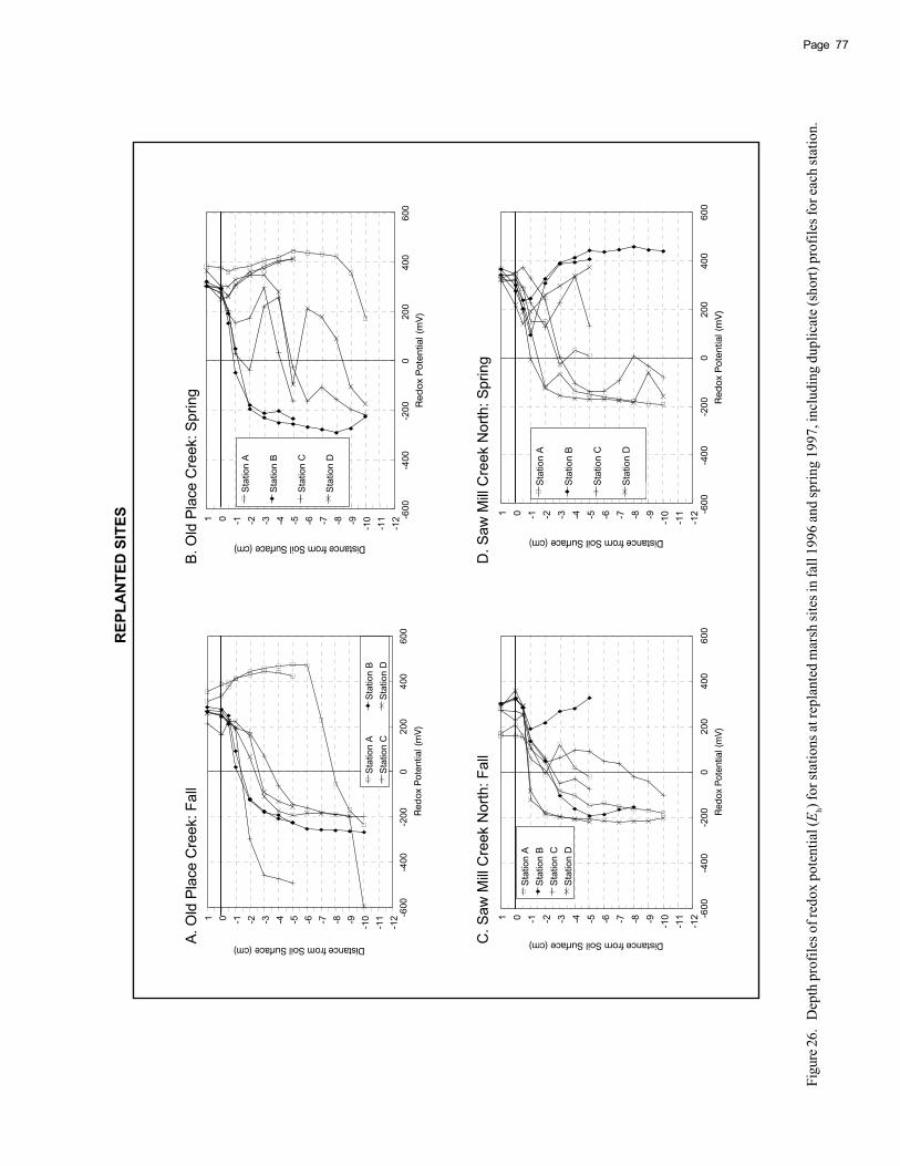
77Page

Figu

re 26

.D

epth

pro

files

of r

edox

pot

entia

l (E h)

for s

tatio

ns at

repl

ante

d m

arsh

site

s in

fall

1996

and

sprin

g 19

97, i

nclu

ding

dup

licat

e (sh

ort)

prof

iles f

or ea

ch st

atio

n.

1 0 -1 -2 -3 -4 -5 -6 -7 -8 -9 -10

-11

-12

020

040

060

0-2

00-4

00-6

00

Sta

tion

A

Sta

tion

B

Sta

tion

C

Sta

tion

D

1 0 -1 -2 -3 -4 -5 -6 -7 -8 -9 -10

-11

-12

020

040

060

0-2

00-4

00-6

00

Sta

tion

A

Sta

tion

B

Sta

tion

C

Sta

tion

D

1 0 -1 -2 -3 -4 -5 -6 -7 -8 -9 -10

-11

-12

020

040

060

0-2

00-4

00-6

00

Sta

tion

A

Sta

tion

B

Sta

tion

C

Sta

tion

D

A. O

ld P

lace

Cre

ek: F

all

B. O

ld P

lace

Cre

ek: S

prin

g

C. S

aw M

ill C

reek

Nor

th: F

all

D. S

aw M

ill C

reek

Nor

th: S

prin

g

REP

LAN

TED

SIT

ES

1 0 -1 -2 -3 -4 -5 -6 -7 -8 -9 -10

-11

-12

020

040

060

0-2

00-4

00-6

00

Sta

tion

A

Sta

tion

B

Sta

tion

C

Sta

tion

D

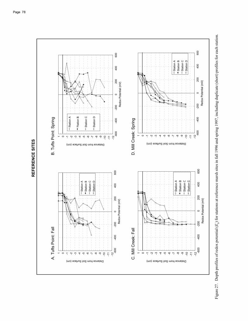
Page 78

Figu

re 27

.D

epth

pro

files

of r

edox

pot

entia

l (E h)

for s

tatio

ns at

refe

renc

e mar

sh si

tes i

n fa

ll 19

96 an

d sp

ring

1997

, inc

ludi

ng d

uplic

ate (

shor

t) pr

ofile

s for

each

stat

ion.

A. T

ufts

Poi

nt: F

all

B. T

ufts

Poi

nt: S

prin

g

C. M

ill C

reek

: Fal

lD

. Mill

Cre

ek: S

prin

g

REF

EREN

CE

SITE

S

1 0 -1 -2 -3 -4 -5 -6 -7 -8 -9 -10

-11

-12

020

040

060

0-2

00-4

00-6

00

Sta

tion

A

Sta

tion

B

Sta

tion

C

Sta

tion

D

1 0 -1 -2 -3 -4 -5 -6 -7 -8 -9 -10

-11

-12

020

040

060

0-2

00-4

00-6

00

Sta

tion

A

Sta

tion

B

Sta

tion

C

Sta

tion

D

1 0 -1 -2 -3 -4 -5 -6 -7 -8 -9 -10

-11

-12

020

040

060

0-2

00-4

00-6

00

Sta

tion

A

Sta

tion

B

Sta

tion

C

Sta

tion

D

1 0 -1 -2 -3 -4 -5 -6 -7 -8 -9 -10

-11

-12

020

040

060

0-2

00-4

00-6

00

Sta

tion

A

Sta

tion

B

Sta

tion

C

Sta

tion

D

79Page

Figu

re 28

.D

epth

pro

files

of r

edox

pot

entia

l (E h)

for s

tatio

ns at

unp

lant

ed m

arsh

site

s in

fall

1996

and

sprin

g 19

97, i

nclu

ding

dup

licat

e (sh

ort)

prof

iles f

or ea

ch st

atio

n.

A. C

on E

d To

wer

: Fal

lB.

Con

Ed

Tow

er: S

prin

g

C. S

aw M

ill C

reek

Sou

th: F

all

D. S

aw M

ill C

reek

Sou

th: S

prin

g

UN

PLA

NTE

D S

ITES

1 0 -1 -2 -3 -4 -5 -6 -7 -8 -9 -10

-11

-12

020

040

060

0-2

00-4

00-6

00

Sta

tion

A

Sta

tion

B

Sta

tion

C

Sta

tion

D

1 0 -1 -2 -3 -4 -5 -6 -7 -8 -9 -10

-11

-12

020

040

060

0-2

00-4

00-6

00

Sta

tion

A

Sta

tion

B

Sta

tion

C

Sta

tion

D

1 0 -1 -2 -3 -4 -5 -6 -7 -8 -9 -10

-11

-12

020

040

060

0-2

00-4

00-6

00

Sta

tion

A

Sta

tion

B

Sta

tion

C

Sta

tion

D

1 0 -1 -2 -3 -4 -5 -6 -7 -8 -9 -10

-11

-12

020

040

060

0-2

00-4

00-6

00

Sta

tion

A

Sta

tion

B

Sta

tion

C

Sta

tion

D

Page 80

Figu

re 29

.Se

ason

al p

atte

rns i

n in

ters

titia

l sol

uble

sulfi

de fr

om re

plan

ted

mar

sh st

atio

ns.

A. O

ld P

lace

Cre

ekB

. Saw

Mill

Cre

ek N

orth

REP

LAN

TED

SIT

ES

2 0 -2 -4 -6 -8 -10

-12

-14

-16

DISTANCE fm SOIL SURFACE (cm)

050

010

0015

0020

0025

0030

00S

OLU

BLE

SU

LFID

E C

ON

CE

NTR

ATI

ON

(μM

)

Fall:

Sta

CS

prin

g: S

ta A

Spr

ing:

Sta

B

>=

SP

RIN

G R

AN

GE

2 0 -2 -4 -6 -8 -10

-12

-14

-16

DISTANCE FROM SOIL SURFACE (cm)0

500

1000

1500

2000

2500

3000

SO

LUB

LE S

ULF

IDE

CO

NC

EN

TRA

TIO

N (μ

M)

Fall:

Sta

CS

prin

g: S

ta A

Spr

ing:

Sta

B

>=

SP

RIN

G R

AN

GE

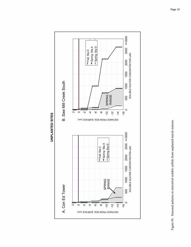
81Page

Figu

re 3

0.Se

ason

al p

atte

rns i

n in

ters

titia

l sol

uble

sulfi

de fr

om u

npla

nted

mar

sh st

atio

ns.

A. C

on E

d To

wer

B. S

aw M

ill C

reek

Sou

th

UN

PLA

NTE

D S

ITES

2 0 -2 -4 -6 -8 -10

-12

-14

-16

DISTANCE FROM SOIL SURFACE (cm)

050

010

0015

0020

0025

0030

00S

OLU

BLE

SU

LFID

E C

ON

CE

NTR

ATI

ON

(μM

)

Fall:

Sta

CS

prin

g: S

ta A

Spr

ing

Sta

D

>=

SP

RIN

G R

AN

GE

2 0 -2 -4 -6 -8 -10

-12

-14

-16

DISTANCE FROM SOIL SURFACE (cm)0

500

1000

1500

2000

2500

3000

SO

LUB

LE S

ULF

IDE

CO

NC

EN

TRA

TIO

N (μ

M)

Fall:

Sta

DS

prin

g: S

ta A

Spr

ing:

Sta

D

>=

SP

RIN

G R

AN

GE

Page 82

Figu

re 31

.Se

ason

al p

atte

rns i

n in

ters

titia

l sol

uble

sulfi

de fr

om re

fere

nce

mar

sh st

atio

ns.

A. T

ufts

Poi

ntB

. Mill

Cre

ek

REF

EREN

CE

SITE

S 2 0 -2 -4 -6 -8 -10

-12

-14

-16

DISTANCE FROM SOIL SURFACE (cm)0

500

1000

1500

2000

2500

3000

SO

LUB

LE S

ULF

IDE

CO

NC

EN

TRA

TIO

N (μ

M)

Fall:

Sta

CS

prin

g: S

ta A

Spr

ing:

Sta

C

>=

SP

RIN

G R

AN

GE

2 0 -2 -4 -6 -8 -10

-12

-14

-16

DISTANCE FROM SOIL SURFACE (cm)

050

010

0015

0020

0025

0030

00S

OLU

BLE

SU

LFID

E C

ON

CE

NTR

ATI

ON

(μM

)

Fall:

Sta

DS

prin

g: S

ta A

Spr

ing:

Sta

C

>=

SP

RIN

G R

AN

GE

83Page

Figu

re 32

.Se

ason

al v

alue

s of

TOC

in su

rfac

e sed

imen

ts ar

rang

ed b

y st

atio

n, si

te, a

nd re

plan

ting

treat

men

t. (C

ET =

Con

Ed

Tow

er; M

C =

Mill

Cre

ek; O

P =

Old

Pla

ce C

reek

;SM

N =

Saw

Mill

Cre

ek N

orth

; SM

S =

Saw

Mill

Cre

ek S

outh

; and

TP

= Tu

fts P

oint

.)

OP-AOP-BOP-COP-D

SMN-ASMN-BSMN-CSMN-D

CET-ACET-BCET-CCET-D

SMS-ASMS-BSMS-CSMS-D

TP-ATP-BTP-CTP-D

MC-AMC-BMC-CMC-D

0102030405060Fa

ll '9

6Sp

ring

'97

Unp

lant

edR

efer

ence

Rep

lant

ed

Site

-Sta

tion

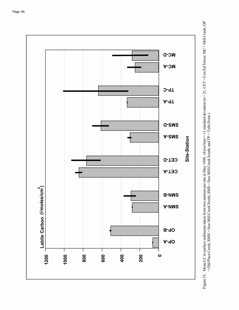
Page 84

Figu

re 33

.M

ean

LC in

surfa

ce se

dim

ents

take

n fro

m tw

o sta

tions

per

site

in M

ay 1

998.

(Er

ror b

ars =

±1

stand

ard

devi

atio

n (n

= 2

). C

ET =

Con

Ed

Tow

er; M

C =

Mill

Cre

ek; O

P=

Old

Pla

ce C

reek

; SM

N =

Saw

Mill

Cre

ek N

orth

; SM

S =

Saw

Mill

Cre

ek S

outh

; and

TP

= Tu

fts P

oint

.)

OP-A

OP-B

SMN-A

SMN-B

CET-A

CET-D

SMS-A

SMS-D

TP-A

TP-C

MC-A

MC-D

Site

-Sta

tion

0

200

400

600

800

1000

1200

Labi

le C

arbo

n (

mol

es/c

m )3

85Page

Figu

re 34

.Lo

g 10 so

lubl

e sul

fide (

in m

M) p

lotte

d ag

ains

t mea

n re

dox

pote

ntia

l (E h i

n m

V) f

or al

l non

zero

sulfi

de v

alue

s gro

uped

by

mar

sh re

plan

ting

stat

us.

010

020

030

040

0-1

00-2

00-3

00

01234 -1

Trea

tmen

tR

epla

nted

Ref

eren

ceU

npla

nted

Ref

eren

cer=

0.6

824

Rep

lant

edr=

0.8

919

Unp

lant

edr=

0.8

628

Page 86

Figu

re 35

.R

elat

ions

hip

betw

een

sedi

men

t sur

face

TO

C an

d si

lt/cl

ay co

nten

t. (A

= re

fere

nce l

ine d

efin

ed b

y eq

uatio

n, %

TOC

= 0

.20

× %

silt/

clay

; B =

regr

essi

on o

f Old

Pla

ceC

reek

dat

a -- b

oth

sprin

g an

d fa

ll --

and

Mill

Cre

ek sp

ring

data

; OP

= O

ld P

lace

Cre

ek; a

nd M

C =

Mill

Cre

ek. O

ld P

lace

Cre

ek -

Stat

ion

C in

May

(circ

led)

lies

out

side

of th

e zo

ne d

elin

eate

d by

all

othe

r Old

Pla

ce C

reek

stat

ion-

seas

on c

ombi

natio

ns.

Con

Ed

Tow

er d

ata

are

not p

lotte

d du

e to

lack

of g

rain

size

dat

a. G

rain

size

dat

aar

e fro

m C

hapt

er II

, “Tr

ace M

etal

Con

tam

inan

ts in

Sed

imen

ts an

d R

ibbe

d-M

usse

ls.”

)

020

4060

8010

005101520

....F

all '

96

....S

prin

g '9

7

OP-

C M

ay

MC

-D S

ep &

May

MC

-C M

ay

MC

-A M

ay

OP

A

B

Ta

ble

12

.A

rth

ur

Kil

l m

ars

h b

iog

eo

ch

em

istr

y b

y t

reatm

en

t, s

ite

, st

ati

on

, an

d s

easo

n

Bio

ge

och

em

ica

l F

ac

tor

hM

ed

ian

EM

ed

ian

Su

lfid

eS

urfa

ce T

OC

Su

rfa

ce L

C

(mV

)(μ

M)

(% o

f d

ry

wt.

)(μ

M/c

m)

3

Tr

ea

tme

nt

Sit

eS

tati

on

Fa

llS

prin

gF

all

Sp

rin

gF

all

Sp

rin

gS

prin

g

Re

pla

nte

dO

ld P

lace

Cre

ek

A+

41

0+

38

20

0.1

80

.11

65

B-1

75

-20

35

70

1.2

52

.57

50

9

C-6

3+

15

2>

30

00

0.3

78

.05

D-9

1+

30

20

.84

1.2

0

Saw

Mil

l C

reek

No

rth

A+

9+

90

9.8

17

.78

28

2

B+

21

7+

38

70

7.1

38

.37

29

5

C+

65

+2

27

14

07

.30

7.8

5

D-1

95

+1

91

6.0

66

.17

Un

pla

nte

dC

on

Ed

To

wer

A-1

57

+2

21

04

5.5

84

2.7

28

46

B-1

41

+1

10

48

.59

15

.69

C+

10

3-3

96

81

0.6

98

.41

D-1

40

+2

62

33

4.1

51

3.4

77

67

Saw

Mil

l C

reek

So

uth

A-1

27

-15

99

26

.19

7.6

93

06

B-1

17

-11

05

.52

7.3

9

C+

46

+2

15

.43

6.6

1

D-1

60

+1

07

10

00

14

6.0

17

.82

61

3

Re

fere

nc

eT

uft

s P

oin

t A

-13

7+

12

51

25

09

.45

6.3

43

35

B-4

3+

11

29

.24

7.2

0

C+

18

1+

16

51

11

.73

13

.13

64

0

D+

13

5+

71

81

13

.81

12

.11

Mil

l C

reek

A+

88

+1

06

12

19

.50

16

.17

25

1

B-1

09

-36

7.8

81

0.7

4

C-1

53

-10

58

20

90

7.7

11

7.4

3

D-1

90

+2

89

.09

9.0

42

84

87Page

Page 88

89Page

V. AGE, GROWTH, AND ALLOMETRIC RELATIONSHIPSOF RIBBED-MUSSELS (Geukensia demissa)

Joseph J. Vitaliano17, 18 and Allen J. Bejda17, 19

Postal Address: 17National Marine Fisheries Serv., 74 Magruder Rd., Highlands, NJ 07732E-Mail Addresses: 18Joseph.Vitaliano@noaa.gov; 19Allen.Bejda@noaa.gov

mussel population. Mussels were also needed for determi-nation of trace metals and hydrocarbon concentrations inthe mussel meats (see “Methods” in Chapters II, “TraceMetal Contaminants in Sediments and Ribbed-Mussels,”and III, “Petroleum Hydrocarbons in Sediments and Ribbed-Mussels). To minimize damage to the replanted marsh sitesand also to the unplanted and reference sites in the alreadyimpacted Arthur Kill, we attempted to make a single musselcollection at each site based on the sampling protocolsneeded for contaminant analysis of mussels. The musselshells would be used for age and growth determinations,and the mussel meats would be used for contaminant analy-ses. This attempt failed to yield adequate numbers of mus-sels and it was necessary to make another collection for theage-and-growth portion of the study.

A minimum of 60 ribbed-mussels were randomly col-lected at each of the six sites during September 1996. At thereference sites, dense aggregations of mussels were foundwithin a narrow area in the S. alterniflora zone. At theunplanted sites, mussels were sparse and had to be col-lected from both vegetated and unvegetated locations overa much larger area of the marsh and undoubtedly from dif-ferent tidal levels. At the replanted sites, sampling wasrestricted to areas within the replanted zone, but away frompermanent quadrats set up by SMRT to monitor the S.alterniflora.

In the laboratory, the sediment, epiphytes, and byssalthreads were removed from each shell, the mussel wasopened, and its tissue was removed. Dry weights for bothshell and tissue were determined after drying to a constantweight at 60°C. After weighing, each mussel was measuredwith vernier calipers to determine shell length (maximumanterior-posterior dimension), width (maximum lateral di-mension), and height (maximum dorsal-ventral dimension).Each mussel was aged by counting external growth rings(annuli). Length at age was determined by measuring themaximum anterior-posterior dimension at each annulus.

RESULTS

The information presented below summarizes the mea-surements made on mussels collected from each site. Since

INTRODUCTION

The ribbed-mussel is a dominant species in tidal saltmarshes of the eastern United States. This bivalve mol-lusk attaches by byssal threads to the stems and roots ofS. alterniflora and other substrates, and is usually mostabundant within the tall S. alterniflora along the marshedge (Bertness 1984). The ribbed-mussel enhances thesurvival of S. alterniflora by binding the root mat to-gether, effectively stabilizing the substrate and strength-ening the plant and the entire marsh against erosion(Bertness 1984). The ribbed-mussel also plays a majorrole in the food web and in the cycling of carbon, nutri-ents, and minerals through the saltmarsh ecosystem. Thisbivalve is a filter feeder on phytoplankton and suspendeddetritus (much of which is dead S. alterniflora), and aconsiderable amount of its fecal matter is deposited onthe marsh surface. The ribbed-mussel is preyed upon byblue crabs (Callinectes sapidus), other crustaceans, gas-tropods, and birds (Bertness 1980, 1984).

Since ribbed-mussels are important in the ecology oftidal salt marshes, site-specific differences in abundance,biomass, age structure, growth rate, and the allometric rela-tionships of ribbed-mussel populations can be explored asindicators of the success of marsh replanting. Samplingproblems and restrictions, however, prevented us from quan-titatively sampling the populations of ribbed-mussels atour replanted, unplanted, and reference sites in the ArthurKill. We will therefore restrict data presentation and analy-sis to descriptive comparisons of several variables basedon measurements of mussels taken from each site.

METHODS AND MATERIALS

A preferred method to sample ribbed-mussel popula-tions quantitatively is to place quadrats of known dimen-sions randomly at similar tidal heights within the S.alterniflora zone at each site (Bertness 1980). The musselsare then destructively removed from each quadrat for enu-meration and measurement. This sampling protocol couldnot be implemented in this study. We were not allowed todestructively sample directly in the replanted areas with themagnitude required to obtain quantitative samples of the

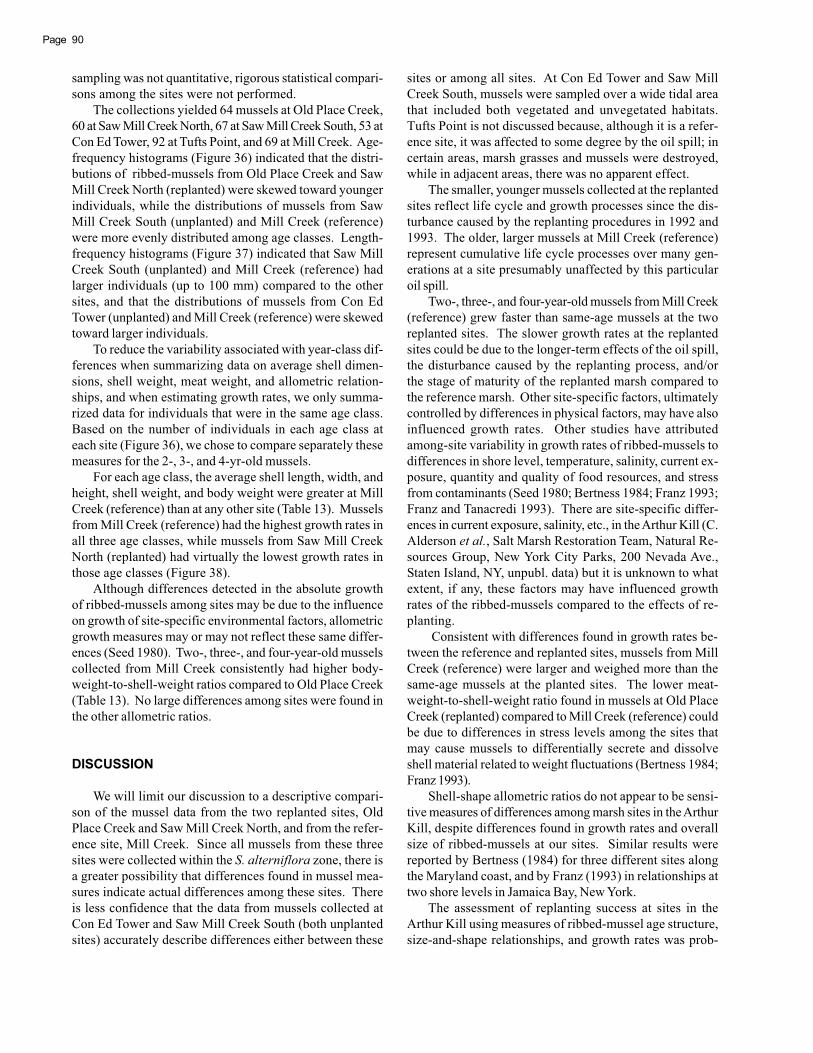
Page 90

sampling was not quantitative, rigorous statistical compari-sons among the sites were not performed.

The collections yielded 64 mussels at Old Place Creek,60 at Saw Mill Creek North, 67 at Saw Mill Creek South, 53 atCon Ed Tower, 92 at Tufts Point, and 69 at Mill Creek. Age-frequency histograms (Figure 36) indicated that the distri-butions of ribbed-mussels from Old Place Creek and SawMill Creek North (replanted) were skewed toward youngerindividuals, while the distributions of mussels from SawMill Creek South (unplanted) and Mill Creek (reference)were more evenly distributed among age classes. Length-frequency histograms (Figure 37) indicated that Saw MillCreek South (unplanted) and Mill Creek (reference) hadlarger individuals (up to 100 mm) compared to the othersites, and that the distributions of mussels from Con EdTower (unplanted) and Mill Creek (reference) were skewedtoward larger individuals.

To reduce the variability associated with year-class dif-ferences when summarizing data on average shell dimen-sions, shell weight, meat weight, and allometric relation-ships, and when estimating growth rates, we only summa-rized data for individuals that were in the same age class.Based on the number of individuals in each age class ateach site (Figure 36), we chose to compare separately thesemeasures for the 2-, 3-, and 4-yr-old mussels.

For each age class, the average shell length, width, andheight, shell weight, and body weight were greater at MillCreek (reference) than at any other site (Table 13). Musselsfrom Mill Creek (reference) had the highest growth rates inall three age classes, while mussels from Saw Mill CreekNorth (replanted) had virtually the lowest growth rates inthose age classes (Figure 38).

Although differences detected in the absolute growthof ribbed-mussels among sites may be due to the influenceon growth of site-specific environmental factors, allometricgrowth measures may or may not reflect these same differ-ences (Seed 1980). Two-, three-, and four-year-old musselscollected from Mill Creek consistently had higher body-weight-to-shell-weight ratios compared to Old Place Creek(Table 13). No large differences among sites were found inthe other allometric ratios.

DISCUSSION

We will limit our discussion to a descriptive compari-son of the mussel data from the two replanted sites, OldPlace Creek and Saw Mill Creek North, and from the refer-ence site, Mill Creek. Since all mussels from these threesites were collected within the S. alterniflora zone, there isa greater possibility that differences found in mussel mea-sures indicate actual differences among these sites. Thereis less confidence that the data from mussels collected atCon Ed Tower and Saw Mill Creek South (both unplantedsites) accurately describe differences either between these

sites or among all sites. At Con Ed Tower and Saw MillCreek South, mussels were sampled over a wide tidal areathat included both vegetated and unvegetated habitats.Tufts Point is not discussed because, although it is a refer-ence site, it was affected to some degree by the oil spill; incertain areas, marsh grasses and mussels were destroyed,while in adjacent areas, there was no apparent effect.

The smaller, younger mussels collected at the replantedsites reflect life cycle and growth processes since the dis-turbance caused by the replanting procedures in 1992 and1993. The older, larger mussels at Mill Creek (reference)represent cumulative life cycle processes over many gen-erations at a site presumably unaffected by this particularoil spill.

Two-, three-, and four-year-old mussels from Mill Creek(reference) grew faster than same-age mussels at the tworeplanted sites. The slower growth rates at the replantedsites could be due to the longer-term effects of the oil spill,the disturbance caused by the replanting process, and/orthe stage of maturity of the replanted marsh compared tothe reference marsh. Other site-specific factors, ultimatelycontrolled by differences in physical factors, may have alsoinfluenced growth rates. Other studies have attributedamong-site variability in growth rates of ribbed-mussels todifferences in shore level, temperature, salinity, current ex-posure, quantity and quality of food resources, and stressfrom contaminants (Seed 1980; Bertness 1984; Franz 1993;Franz and Tanacredi 1993). There are site-specific differ-ences in current exposure, salinity, etc., in the Arthur Kill (C.Alderson et al., Salt Marsh Restoration Team, Natural Re-sources Group, New York City Parks, 200 Nevada Ave.,Staten Island, NY, unpubl. data) but it is unknown to whatextent, if any, these factors may have influenced growthrates of the ribbed-mussels compared to the effects of re-planting.

Consistent with differences found in growth rates be-tween the reference and replanted sites, mussels from MillCreek (reference) were larger and weighed more than thesame-age mussels at the planted sites. The lower meat-weight-to-shell-weight ratio found in mussels at Old PlaceCreek (replanted) compared to Mill Creek (reference) couldbe due to differences in stress levels among the sites thatmay cause mussels to differentially secrete and dissolveshell material related to weight fluctuations (Bertness 1984;Franz 1993).

Shell-shape allometric ratios do not appear to be sensi-tive measures of differences among marsh sites in the ArthurKill, despite differences found in growth rates and overallsize of ribbed-mussels at our sites. Similar results werereported by Bertness (1984) for three different sites alongthe Maryland coast, and by Franz (1993) in relationships attwo shore levels in Jamaica Bay, New York.

The assessment of replanting success at sites in theArthur Kill using measures of ribbed-mussel age structure,size-and-shape relationships, and growth rates was prob-

91Page

lematic due to sampling difficulties, and was confoundedby site-specific differences in environmental factors. De-pressed growth rates and sizes in mussels of the same agemay be typical of the northern reaches of the Arthur Kill[Old Place Creek and Saw Mill Creek North (replanted)] com-pared to the southern areas [Mill Creek (reference)].

REFERENCES CITED

Bertness, M.D. 1980. Growth and mortality in the ribbed-mussel, Geukensia demissa. Veliger 23:62-69.

Bertness, M.D. 1984. Ribbed-mussels and Spartinaalterniflora production in a New England salt marsh.Ecology 64:1794-1807.

Franz, D.R. 1993. Allometry of shell and body weight inrelation to shore level in the intertidal bivalveGeukensia demissa (Bivalvia: Mytilidae). J. Exp. Mar.Biol. Ecol. 174:193-207.

Franz, D.R.; Tanacredi, J.T. 1993. Variability in growth andage structure among populations of ribbed-mussels,Geukensia demissa (Dillwyn) (Bivalvia: Mytilidae), inJamaica Bay, New York (Gateway NRA). Veliger36:220-227.

Seed, R. 1980. Shell growth and form in the Bivalvia. In:Rhoads, D.; Lutz, R., eds. Skeletal growth of aquaticorganisms. New York, NY: Plenum Press; p. 23-65.

OLD PLACE

05

101520253035

1 2 3 4 5 6 7 8 9 10 11AGE

NU

MB

ER O

F M

USS

ELS

N = 64

SAW MILL NORTH

05

101520253035

1 2 3 4 5 6 7 8 9 10 11AGE

NU

MB

ER O

F M

USS

ELS

N = 60

SAW MILL SOUTH

05

101520253035

1 2 3 4 5 6 7 8 9 10 11AGE

NU

MB

ER O

F M

USS

ELS

N = 67

CON ED TOWER

0

5

10

15

20

25

30

35

1 2 3 4 5 6 7 8 9 10 11

AGE

NU

MB

ER O

F M

USS

ELS

N = 53

TUFTS POINT

05

101520253035

1 2 3 4 5 6 7 8 9 10 11AGE

NU

MB

ER O

F M

USS

ELS

N = 92

MILL CREEK

05

101520253035

1 2 3 4 5 6 7 8 9 10 11

AGE

NU

MB

ER O

F M

USS

ELS

N = 69

Page 92

Figure 36. Age-frequency distribution of ribbed-mussels collected at Old Place Creek and Saw Mill Creek North (replanted),Saw Mill Creek South and Con Ed Tower (unplanted), and Tufts Point and Mill Creek (reference) in September1996.

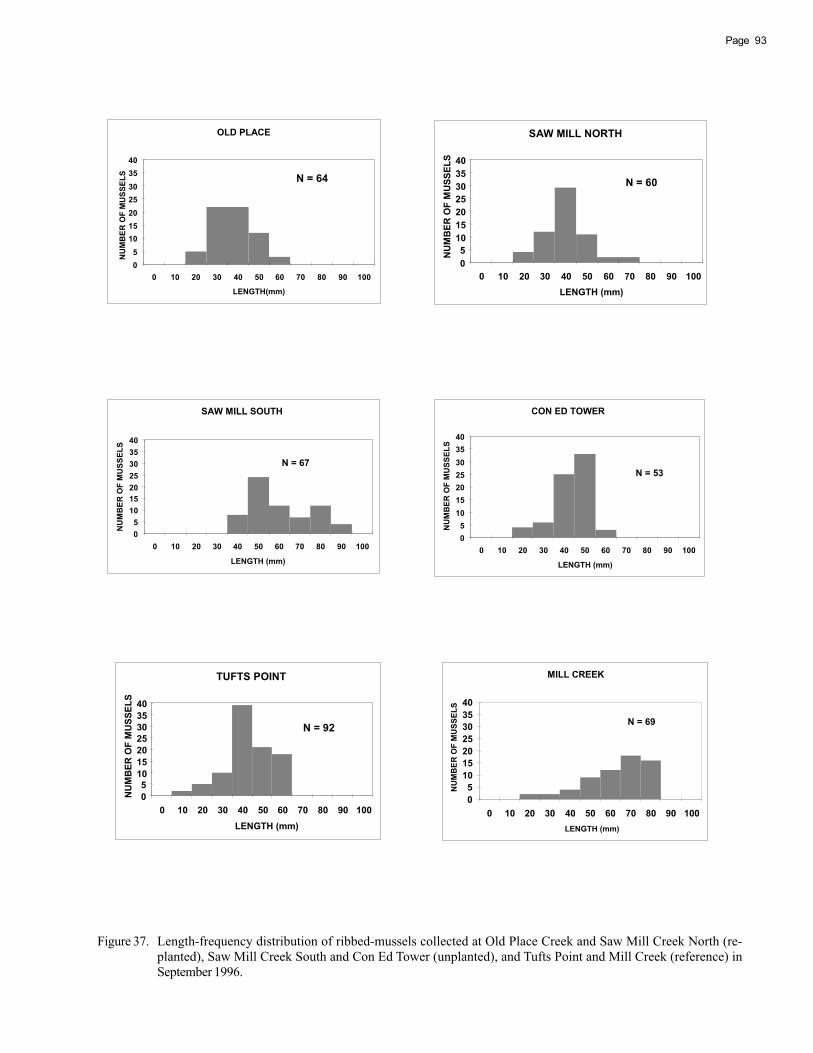
OLD PLACE

05

10152025303540

0 10 20 30 40 50 60 70 80 90 100

LENGTH(mm)

NU

MB

ER O

F M

USS

ELS N = 64

SAW MILL NORTH

05

10152025303540

0 10 20 30 40 50 60 70 80 90 100LENGTH (mm)

NU

MB

ER O

F M

USS

ELS

N = 60

SAW MILL SOUTH

05

10152025303540

0 10 20 30 40 50 60 70 80 90 100

LENGTH (mm)

NU

MB

ER O

F M

USS

ELS

N = 67

TUFTS POINT

05

10152025303540

0 10 20 30 40 50 60 70 80 90 100LENGTH (mm)

NU

MB

ER O

F M

USS

ELS

N = 92

MILL CREEK

05

10152025303540

0 10 20 30 40 50 60 70 80 90 100LENGTH (mm)

NU

MB

ER O

F M

USS

ELS

N = 69

CON ED TOWER

05

10152025303540

0 10 20 30 40 50 60 70 80 90 100

LENGTH (mm)

NU

MB

ER O

F M

USS

ELS

N = 53

93Page

Figure 37. Length-frequency distribution of ribbed-mussels collected at Old Place Creek and Saw Mill Creek North (re-planted), Saw Mill Creek South and Con Ed Tower (unplanted), and Tufts Point and Mill Creek (reference) inSeptember 1996.

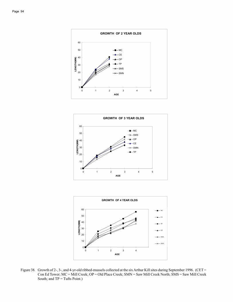
GROWTH OF 2 YEAR OLDS

0

10

20

30

40

50

60

0 1 2 3 4 5

AGE

LEN

GTH

(MM

)

MC

CE

OP

TP

SMS

SMN

GROWTH OF 3 YEAR OLDS

0

10

20

30

40

50

60

0 1 2 3 4 5

AGE

LEN

GTH

(MM

)

MC

SMS

OP

CE

SMN

TP

GROWTH OF 4 YEAR OLDS

0

10

20

30

40

50

60

0 1 2 3 4

AGE

LEN

GTH

(MM

)

MC

CE

TP

OP

SMS

SMN

Page 94

Figure 38. Growth of 2-, 3-, and 4-yr-old ribbed-mussels collected at the six Arthur Kill sites during September 1996. (CET =Con Ed Tower; MC = Mill Creek; OP = Old Place Creek; SMN = Saw Mill Creek North; SMS = Saw Mill CreekSouth; and TP = Tufts Point.)

95Page

Tabl

e 13

.A

vera

ge sh

ell d

imen

sion

s, sh

ell d

ry w

eigh

t, m

eat d

ry w

eigh

t, an

d sh

ell s

hape

and

bod

y si

ze re

latio

nshi

ps fo

r 2-,

3-, a

nd 4

-yr-

old

ribbe

d-m

usse

ls c

olle

cted

at t

hesi

x A

rthur

Kill

site

s dur

ing

Sept

embe

r 199

6.

Allo

met

ric

Rel

atio

nshi

pPh

ysic

al M

easu

reSh

ell H

eigh

t/Sh

ell

Shel

lSh

ell

Shel

lM

eat D

ryM

eat D

ry W

eigh

tSh

ell W

idth

Shel

l Hei

ght

Shel

l Wid

thN

o. o

fL

engt

hW

idth

Hei

ght

Wei

ght

Wei

ght

vs.

vs.

vs.

vs.

Site

Sam

ples

(mm

)(m

m)

(mm

)(g

)(g

)Sh

ell W

eigh

tSh

ell L

engt

hSh

ell L

engt

hSh

ell L

engt

h

Age

2

Old

Pla

ce C

reek

2331

.719

.813

.33.

010.

150.

049

0.63

0.42

0.02

1Sa

w M

ill C

reek

Nor

th21

28.0

20.9

14.3

3.10

0.17

0.05

60.

750.

510.

025

Saw

Mill

Cre

ek S

outh

1130

.123

.315

.43.

530.

220.

064

0.77

0.51

0.02

2C

on E

d To

wer

838

.023

.216

.54.

520.

230.

052

0.61

0.44

0.01

9Tu

fts P

oint

1230

.319

.813

.53.

090.

150.

050

0.65

0.44

0.02

2M

ill C

reek

740

.426

.519

.16.

300.

580.

087

0.66

0.47

0.01

8

Age

3

Old

Pla

ce C

reek

1537

.921

.815

.14.

070.

180.

045

0.58

0.40

0.01

8Sa

w M

ill C

reek

Nor

th13

33.6

21.6

14.3

3.15

0.18

0.05

70.

640.

420.

020

Saw

Mill

Cre

ek S

outh

941

.326

.517

.95.

210.

390.

073

0.64

0.43

0.01

6C

on E

d To

wer

437

.321

.316

.84.

950.

210.

044

0.57

0.45

0.02

1Tu

fts P

oint

3032

.919

.213

.83.

000.

140.

049

0.58

0.42

0.02

2M

ill C

reek

844

.927

.820

.26.

760.

460.

066

0.62

0.45

0.01

6

Age

4

Old

Pla

ce C

reek

143

.022

.615

.44.

420.

210.

046

0.52

0.36

0.01

6Sa

w M

ill C

reek

Nor

th9

37.2

22.4

14.8

3.36

0.20

0.06

10.

600.

400.

018

Saw

Mill

Cre

ek S

outh

1041

.627

.619

.66.

320.

380.

060

0.66

0.47

0.01

7C

on E

d To

wer

2046

.123

.216

.94.

590.

230.

052

0.50

0.37

0.01

6Tu

fts P

oint

1844

.523

.316

.84.

990.

240.

051

0.52

0.38

0.01

6M

ill C

reek

1056

.130

.822

.49.

530.

620.

064

0.55

0.40

0.01

3

Page 96

97Page

VI. BENTHIC INVERTEBRATES

Joseph J. Vitaliano20, 22, Robert N. Reid20, 23, Ann B. Frame20,David B. Packer20, 24, Linda Arlen20, 25, and John N. Sacco21, 26

Postal Addresses: 20National Marine Fisheries Serv., 74 Magruder Rd., Highlands, NJ 07732; 21NewJersey Dept. of Environmental Protection, 501 E. State St., P.O. Box 404, Trenton,NJ 08625-0404

E-Mail Addresses: 22Joseph.Vitaliano@noaa.gov; 23Robert.Reid@noaa.gov; 24Dave.Packer@noaa.gov;25Linda.Arlen@noaa.gov; 26John.Sacco@dep.state.nj.us

the saltmarsh ecosystem (Sacco et al. 1994; Levin et al.1998), a 0.3-mm sieve was used in this study to retain aportion of these smaller invertebrates. Both the meiofaunaand macrofauna retained on the 0.3-mm sieve will be re-ferred to as “benthic invertebrates.”

RESULTS

Forty-one taxa were identified in the study collections.Oligochaetes were the most abundant taxon, comprising60% of all individuals counted. Nematodes were the nextmost abundant taxon, comprising 20% of all individualscounted, followed by the small tube-building fan worm,Manayunkia aestuarina, comprising 14% of all individualscounted. Together these three taxa made up approximately94% of all individuals in the samples. Although most of theindividuals found are considered meiofauna, juveniles oflarger invertebrates, including the ribbed-mussel, were alsopresent. Larger amphipods, isopods, and aquatic insectswere found at most sites (Table 14).

There were greater mean abundances of benthic inver-tebrate individuals at all sites in the May samples comparedto the September samples. Oligochaetes contributed mostto this seasonal increase, except at Con Ed Tower(unplanted) where nematodes contributed the most, and atSaw Mill Creek North (replanted) where M. aesturina con-tributed the most. In the September survey, M. aesturinawas found in greatest abundance at Con Ed Tower, while inthe May survey, it was found in greatest abundances at thereplanted sites Old Place Creek and Saw Mill Creek North.In September, Old Place Creek had the largest numbers oftaxa (19), while both Con Ed Tower and Sawmill Creek South(unplanted) had the lowest numbers of taxa (10); in May,there were 22 taxa at Tufts Point (reference) and only eighttaxa at Sawmill Creek North (Table 15).

DISCUSSION

The invertebrate taxa found at the six marsh sites (Table15) appear to be typical of invertebrates found in tidal S.alterniflora marshes elsewhere. Most of these inverte-brates increase in abundance in late spring to early summer,

INTRODUCTION

Benthic invertebrates are important members of thesaltmarsh ecosystem since they are part of detrital foodwebs linking marsh productivity to resource species (Moyand Levin 1991; Minello and Zimmerman 1992). The effectsof oil or its components on invertebrates and their habitatsare well documented (Saunders et al. 1980; Suchanek 1993;Burger 1994; Jewett et al. 1999). There is also considerableinformation available on the benthic invertebrates of cre-ated salt marshes compared to those of nearby naturalmarshes (Moy and Levin 1991; Minello and Zimmerman1992; Sacco et al. 1994; Levin et al. 1996). Little informationis available, however, about the benthic invertebrate as-semblages at restored S. alterniflora marshes that were notonly destroyed by an oil spill, but also historically affectedby petroleum products, trace metals, and other contami-nants similar to the sites studied in the Arthur Kill.

METHODS AND MATERIALS

Sampling methods for benthic invertebrates followthose of Sacco et al. (1994). A 3-cm-diameter (7 cm2) metalcoring tube was used to collect 5-cm-deep sediment samplesfrom the marsh surface. During each sampling month andat low tide, two core samples were taken at each of the fourstations along the transect at each site, for a total of eightcore samples per site per sampling month. Sediments andbiota were removed from the core and fixed in 10% bufferedFormalin in seawater with rose bengal added to aid in sort-ing and identification of the invertebrates. Prior to sorting,samples were sieved through a 0.3-mm stainless steel sieve.The retained sediments and invertebrates were transferredto 70% ethanol with 5% glycerin, and were examined usingdissecting microscopes. All organisms were removed, iden-tified to the lowest practicable taxonomic level, and counted.

Benthic invertebrates are often divided by size and/ortaxonomy into: 1) meiofauna (usually defined as organismspassing through a 0.5-mm-mesh sieve, and dominated bynematodes, harpactacoid copepods, oligochaetes, and smallpolychaetes); or 2) macrofauna (larger polychaetes, crusta-ceans, mollusks, echinoderms, etc.) that are retained on the0.5-mm sieve. Since oligochaetes are important members of

Page 98

and decrease in abundance in late summer to early fall(Tables 14 and 15). Predation, species-specific reproduc-tive strategies, and the availability of food are importantinteractive factors controlling fluctuations in densities (Rader1984; Moy and Levin 1991; Minello and Zimmerman 1992;Sacco et al. 1994; Sarda et al. 1994, 1995, 1998; Levin et al.1996, 1998; Posey et al. 1997).

The variability in the data, which is typical of benthicinvertebrate studies, the site-specific differences, and thelow number of sites sampled confounded the determinationof the effect of replanting of S. alterniflora on benthic in-vertebrate abundances in the Arthur Kill. Similarities wereobserved, however, in the abundances of all invertebrates,oligochaetes, and M. aestuarina between the replanted site,Old Place Creek, and at the reference site, Tufts Point, bothin September and May (Table 15). Although these prelimi-nary findings suggest, in terms of benthic fauna, structuralsimilarities between the replanted and reference sites in theArthur Kill, the functional equivalency of these marsh sitescould not be determined.

REFERENCES CITED

Burger, J. 1994. Immediate effects of oil spills on organisms inthe Arthur Kill. In: Burger, J., ed. Before & after an oil spill:the Arthur Kill. New Brunswick, NJ: Rutgers Univ. Press;p. 115-129.

Jewett, S.C.; Dean, T.A.; Smith, R.O.; Blanchard, A. 1999.‘Exxon Valdez’ oil spill: impacts and recovery in soft bot-tom benthic community in and adjacent to eelgrass beds.Mar. Ecol. Prog. Ser. 185:59-83.

Levin, L.; Tally, D.; Thayer, G. 1996. Succession ofmacrobenthos in a created salt marsh. Mar. Ecol. Prog.Ser. 141:67-82.

Levin, L.; Tally, T.S.; Hewitt, J. 1998. Macrobenthos of Spartinafoliosa (Pacific cordgrass) salt marshes in southern Cali-

fornia: community structure and comparison to a Pacificmudflat and a Spartina alterniflora (Atlantic smoothcordgrass) marsh. Estuaries 21:129-144.

Minello, T.J.; Zimmerman, R.J. 1992. Utilization of natural andtransplanted Texas salt marshes by fish and decapod crus-taceans. Mar. Ecol. Prog. Ser. 90:273-285.

Moy, L.D.; Levin, L.A. 1991. Are Spartina marshes a replace-able resource? A functional approach to evaluation ofmarsh creation efforts. Estuaries 14:1-16.

Posey, M.H.; Alphin, T.D.; Powell, C.M. 1997. Plant and infau-nal communities associated with a created marsh. Estuar-ies 20:42-47.

Rader, D.N. 1984. Salt-marsh benthic invertebrates: small-scale patterns of distribution and abundance. Estuaries7:413-420.

Sacco, J.N.; Seneca, E.D.; Wentworth, T.R. 1994. Infaunalcommunity development of artificially established saltmarshes in North Carolina. Estuaries 17:489-500.

Sarda, R.; Forman, K.; Valiela, I. 1994. Long-term changes ofmacroinfaunal assemblages in experimentally enriched saltmarsh tidal creeks. Biol. Bull. (Woods Hole) 187:282-283.

Sarda, R.; Forman, K.; Valiela, I. 1995. Macroinfauna of aSouthern New England salt marsh: seasonal dynamicsand production. Mar. Biol. (Berl.) 121:431-445.

Sarda, R.; Forman, K.; Werme, C.E.; Valiela, I. 1998. The impactof epifaunal predation on the structure of macrofaunalinvertebrate communities of tidal saltmarsh creeks. Es-tuarine Coastal Shelf Sci. 46:657-669.

Saunders, H.L.; Grassle, J.F.; Hampson, G.R.; Morse, L.S.; Gar-ner-Price, S.; Jones, C.C. 1980. Anatomy of an oil spill:long-term effects from the grounding of the barge Floridaoff West Falmouth, Massachusetts. J. Mar. Res. 38:265-280.

Suchanek, T.H. 1993. Oil impacts on marine invertebrate popu-lations and communities. Am. Zool. 33:510-533.

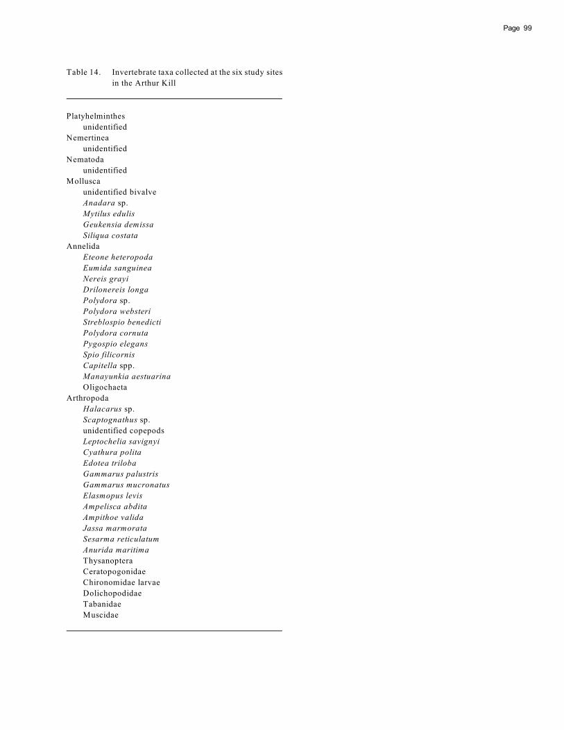
99Page

Table 14. Invertebrate taxa collected at the six study sites

in the Arthur Kill

Platyhelminthes

unidentified

Nemertinea

unidentified

Nematoda

unidentified

Mollusca

unidentified bivalve

Anadara sp.

Mytilus edulis

Geukensia demissa

Siliqua costata

Annelida

Eteone heteropoda

Eumida sanguinea

Nereis grayi

Drilonereis longa

Polydora sp.

Polydora websteri

Streblospio benedicti

Polydora cornuta

Pygospio elegans

Spio filicornis

Capitella spp.

Manayunkia aestuarina

Oligochaeta

Arthropoda

Halacarus sp.

Scaptognathus sp.

unidentified copepods

Leptochelia savignyi

Cyathura polita

Edotea triloba

Gammarus palustris

Gammarus mucronatus

Elasmopus levis

Ampelisca abdita

Ampithoe valida

Jassa marmorata

Sesarma reticulatum

Anurida maritima

Thysanoptera

Ceratopogonidae

Chironomidae larvae

Dolichopodidae

Tabanidae

Muscidae

Page 100

Ta

ble

15

.M

ean

s (+

/- o

ne

sta

nd

ard

de

via

tio

n)/

7-c

m c

ore

(n

= 8

) fo

r th

e a

bu

nd

an

ces

of

all

ben

thic

in

ve

rte

bra

tes,

oli

go

ch

aete

s, n

em

ato

de

s, a

nd

Ma

na

yu

nkia

aestu

arin

a2

at

each

of

the

six

stu

dy

sit

es

an

d t

wo

sam

pli

ng

da

tes

in t

he A

rth

ur

Kil

l.

(Als

o g

iven

are

th

e t

ota

l n

um

ber

of

tax

a i

n a

ll c

ore

s fo

r each

sit

e a

nd

sam

pli

ng

mo

nth

.)

Sit

e

Old

Pla

ce

Sa

w M

ill

Sa

w M

ill

Co

n E

d

Ta

xa

Creek

Creek

No

rth

Creek

So

uth

To

wer

Tu

fts

Po

int

Mil

l C

reek

Sep

tem

be

r 1

99

6

All

in

ve

rte

bra

tes

5

5.8

(2

1.1

)1

4.9

(7

.7)

10

7.8

(3

0.2

)1

55

.3 (

63

.0)

79

.0 (

69

.9)

43

.3 (

20

.7)

Oli

go

ch

aete

s2

1.3

(1

2.7

)3

.6 (

1.7

)8

3.9

(2

2.3

)8

6.5

(3

5.1

)4

8.3

(4

5.0

)2

4.3

(1

3.6

)

Ne

mato

de

s2

.4 (

1.5

)0

11

.4 (

5.7

)1

9.9

(8

.7)

0.4

(0

.4)

5.4

(4

.3)

Ma

na

yu

nkia

aestu

arin

a2

2.3

(1

1.8

)1

.9 (

1.0

)5

.8 (

3.5

)4

6.1

(2

2.5

)2

2.6

(2

2.6

)6

.6 (

3.7

)

To

tal

tax

a1

91

51

01

01

61

5

Ma

y 1

99

7

All

in

ve

rte

bra

tes

27

6.1

(8

5.7

)9

5.0

(3

4.2

)1

89

.4 (

70

.5)

30

0.9

(1

06

.6)

21

5.6

(2

9.3

)1

23

.0 (

36

.8)

Oli

go

ch

aete

s1

85

.8 (

58

.3)

36

.4 (

12

.0)

16

1.4

(6

1.3

)6

7.4

(2

4.7

)1

68

.5 (

23

.7)

10

6.5

(3

1.9

)

Ne

mato

de

s3

2.3

(1

5.2

)1

5.6

(7

.6)

21

.9 (

10

.2)

21

1.0

(9

1.6

)4

.3 (

1.4

)6

.0 (

2.9

)

Ma

na

yu

nkia

aestu

arin

a3

5.3

(1

1.2

)3

9.6

(1

5.2

)4

.9 (

1.4

)1

5.3

(7

.8)

29

.4 (

12

.2)

2.0

(0

.7)

To

tal

tax

a1

28

91

22

21

2

101Page

VII. FOOD HABITS OF THEMUMMICHOG (Fundulus heteroclitus)

Frank W. Steimle, Jr.

Postal Addresses: National Marine Fisheries Serv., 74 Magruder Rd., Highlands, NJ 07732

E-Mail Address: Frank.Steimle@noaa.gov

Gut content analysis can also support and enhance theresults of stable isotope analysis for understanding tro-phodynamics. For example, Kneib et al. (1980) and Hughesand Sherr (1983) used isotopic analysis to show two mainsources of plant carbon being incorporated into mummi-chog tissue, and Griffin and Valiela (2001) used isotopicanalysis to show that the mummichog moves up approxi-mately one step within the benthic trophic food web duringa single growing season, consistent with an increase inlength. Analysis of stomach contents can define the origi-nal and intermediate transfer of these and possibly othersources of plant carbon, as was true for the Griffin andValiela (2001) study. Examination of the diet of the mummi-chog, the most common bottom fish along the marsh fringe,contributes to interpreting algal and benthic invertebratecommunity structures at restoration study sites, as thesestructures can be altered by the feeding of mummichogs(Vince et al. 1976; Kneib and Stiven 1982).

The functional evaluation of restored salt marshes isimportant for the assessment and improvement of restora-tion efforts. Presence or absence of predators such as fish,and variations in their abundances in restored habitats, arevaluable indicators of general habitat suitability, but thesevariables can only suggest that the habitat has recoveredits normal ecological function. Trophic relationships andbiological energy transfers are considered useful functionalendpoints to a restoration, i.e., the diet and feeding of aforage species such as the mummichog can indicate therestoration of an important ecosystem link (Kelly and Harwell1990). In addition, the mummichog is, as Halpin (1997) states,an “excellent model for studying not only the ecology ofsaltmarsh fish but rules governing the invasion of marginalhabitats by mobile animals.”

The mummichog is also an ideal candidate for this studybecause of its assumed fidelity to the study sites. It isthought to have a limited home range, generally <36 m ofshoreline/marsh fringe (Lotrich 1975), although a recentstudy shows that its home range can be quite a bit larger(Sweeney et al. 1998). However, Halpin (1997) shows thatthis species is restricted to areas representing a very smallproportion of the total available habitat; it also displaysfine-scale differences of habitat usage, with patterns of habi-tat usage varying seasonally (Allen et al. 1994), and ap-pears to remain and feed within the small estuaries in whichit was hatched (Griffin and Valiela 2001).

INTRODUCTION

The intertidal salt marsh is used as a source of food orfeeding grounds for a number of estuarine organisms, in-cluding fish and invertebrates. Some of these organismsare in turn prey for larger organisms. The mummichog, orcommon killifish, Fundulus heteroclitus, lives along thesaltmarsh fringe and is generally considered an importantlink in the estuarine food web supporting valued biologicalresources. The mummichog uses the tidally flooded marshto access S. alterniflora stems as a refuge from predation,and to feed on whatever (e.g., detritus, algae, fish larvae,amphipods, tanaids, copepods, and insects) is available(Kneib and Stiven 1978; Weisberg et al. 1981; Werme 1981;Abraham 1985; Moy and Levin 1991; Allen et al. 1994; Kneiband Wagner 1994; Halpin 2000).

Within the ecologically stressed Arthur Kill, the mummi-chog is considered the only widely abundant fish (Howellsand Brundage 1977). It can be an important prey item forprotected wading birds and for larger fish such as Americaneel (Anguilla rostrata), juvenile bluefish (Pomatomussaltatrix), summer flounder, (Paralichthys dentatus), and pos-sibly striped bass (Morone saxatilus) that are common in theArthur Kill area (Rountree and Able 1992; Parsons 1994; Wilket al. 1996). Thus, it serves as an important energy transfermechanism between the Arthur Kill marshes and their adjacentwaters (Valiela et al. 1977; Weisberg and Lotrich 1982; Kneib1986; Kneib and Wagner 1994).

Given the mummichog’s close association with saltmarshes, it is possible that residual effects of the 1990 oilspill, or any differences among the replanted, unplanted, orreference marshes, may be reflected in its diet. The poten-tial or actual impact of oil on fishery resources and theirfood have been recognized since the earliest part of thiscentury (Gutsell 1921), but studies on the interactions be-tween these impacts and habitat restoration have just be-gun. Brzorad and Burger (1994) suggest that the diet of themummichog in the Arthur Kill has been altered in thesepolluted waters by restricting the availability of its prey.However, the mummichog is moderately tolerant of oil con-tamination, except under thermal or osmotic stress (Abraham1985). The mummichog diet can also suggest pathways bywhich oil and other anthropogenic contaminants can betransferred from sediments, substrates, and lower biologi-cal levels of the marsh ecosystem to higher trophic levels.

Page 102

This chapter presents and discusses the results of apreliminary examination of the diets of the mummichogscollected as part of the Arthur Kill study in fall 1996 andspring-summer 1997. The diets of these fish were examinedfor differences which might be correlated with the replant-ing efforts following the 1990 oil spill.

METHODS AND MATERIALS

Fish were collected in September 1996 and between Mayand early August 1997 with standard, tubular, galvanized-wire-mesh killitraps with open funnels at either end, baitedwith either a fish-based, orange-colored, canned cat foodor freshly broken whole northern quahogs (Mercenariamercenaria) or Atlantic surfclams (Spisula solidissima).The bait was contained within ultrafine synthetic meshbags. Some trap samples from the Old Place Creek and ConEd Tower marsh sites were obtained from cooperative col-lections with SMRT; SMRT used bread as bait in their traps.These baits were readily identifiable in the stomachs, thusallowing separation from the other stomach contents whenthe fish actually ingested the bait.

Traps were required for collection as seining was notfeasible because of conditions at most sites. Since theobjective of this study was to examine how mummichogswere using the marshes for feeding, and since the fish mostlyfed in the marsh at high tide, the traps were deployed at themarsh fringe just before high tide. Saltmarsh fringes areconsidered important factors for fish in marsh restorations(Peterson and Turner 1994). The traps were left for 2-3 hrand were retrieved when water had retreated from the marshsurface so that stomach contents of trapped fish wouldbest represent recent feeding on the marsh surface. Butnerand Brattstrom (1960) and Allen et al. (1994) reported thatmummichog stomachs are mostly full at or after high tide.

Upon trap retrieval, at least 30 mummichogs of mixedsizes were removed and preserved in 10% Formalin. Thespring-summer 1997 collections were problematic as an un-usually cool spring seemed to retard the mummichog’s re-turn to all of the marshes, and required an extended collec-tion period to obtain sufficient samples at all sites. In coldermonths, mummichogs tend to remain higher up in creeks orin saltmarsh tide pools (Fritz et al. 1975; Smith and Able1994; Halpin 1997).

In the laboratory, 30 fish were selected from each of thesix sites for both collection periods, for a total of 360 fish.Each set of 30 fish contained 10 each of the largest-, small-est-, and intermediate-sized fish. Fish were measured tototal length and were sexed, then their stomachs and intes-tines were removed and examined under a dissecting micro-scope. The total stomach volume was estimated, then thecontents were examined and separated into definable foodtypes. Organismal prey were identified to the lowest prac-tical taxonomic level, their proportional contribution to the

total volume was visually estimated, and countable itemswere enumerated. Because meiofauna were found in thestomachs, the contents were specifically examined for cope-pods, foraminifera, nematodes, oligochaete fragments, anddiatoms. These latter taxa could provide clues to specificmicrohabitat use, such as feeding on the algal mats grow-ing at the base of S. alterniflora stems (Werme 1981). Avariety of estuarine invertebrate taxonomic keys were usedto identify stomach contents, e.g., Wilson (1932), Gosner(1971), Bousfield (1973), and Weiss (1995). When bait wasdetected in the stomachs, it was noted and the upper intes-tine was also examined in case the bait had pushed naturalfood out of the stomachs. Gastrointestinal evacuation canbe fairly rapid for mummichogs, often on the order of sev-eral hours (C.L. MacKenzie, National Marine Fisheries Serv.,74 Magruder Rd., Highlands, NJ, 07732, pers. comm.).

Comparative analysis of the diets among sites and treat-ments for this preliminary study included the percent fre-quency of occurrence of specific food items or prey in thestomachs, and the estimated mean percentage of total stom-ach volume associated with a specific food item or prey.Numerical analysis was not feasible because of the abun-dance of noncountable material in the stomachs (e.g., detri-tus, algal material). The small sample sizes, especially perfish length class, and the preliminary nature of the study,precluded the use of extensive statistical treatments.

RESULTS

As the focus of this preliminary study is on possibledifferences among collection sites and treatments and noton seasonal or interannual variability, the results for eachcollection period are presented separately.

September 1996

The sizes of the 180 mummichogs examined for this sam-pling period ranged from 3.3-10.5 cm. This size range wasconsistent among sampling sites. The results of the stom-ach content analysis among sites and treatments for thisperiod are presented in Tables 16 and 17.

The data on percent frequency of occurrence (Table 16)shows that detritus was the most commonly occurring ma-terial at all sites and treatments. Algae, both strands (mixedchains of diatoms or variously colored filamentous tubes)and macrophytes, were next in overall, but variable, impor-tance, especially at Con Ed Tower (unplanted), Tufts Point(reference), and Mill Creek (reference) sites. Insects, mostlyfragments of adult forms, but including Diptera larvae, wereeaten at all sites at a low frequency. Decapod shrimp (mostlyPalaemonetes fragments) commonly occurred only at TuftsPoint, while the marsh hopper amphipod, Orchestia grillus,commonly occurred only at Mill Creek. The shrimp

103Page

Palaemonetes sp. was also often collected in the fish trapsat some sites, but was found only in the stomachs of thelarger fish.

The data on mean percent stomach volume (Table 17)show that detritus was less important and occurrence ofbait was more obvious. The use of detritus was highest atthe two northernmost sites, Old Place Creek and Con EdTower. The occurrence of bait in stomachs was generallyhighest at all four oiled sites, and is a sampling artifact,although it may indicate limited food availability. Algalstrands and blades were important at the two reference sites.Again, decapod shrimp were notable only at Tufts Point,while Orchestia grillus was notable only at Mill Creek.Microscopic items in the stomachs (e.g., foraminifera) ap-pear to be minor contributors to the food requirements ofthe mummichog.

May-August 1997

The sizes of the 180 fish examined for this samplingperiod ranged from 3.2 to 9.9 cm, which is similar to theprevious sampling period. The results of the stomach ex-aminations for this period are presented in Tables 18 and 19.

The most frequently occurring item was amphipod frag-ments, probably Gammarus sp., with detritus being next infrequency; detritus was less frequent at the two referencesites (Table 18). Insects again and nematodes occurred atall sites. Algal strands were found only at the unplantedand reference sites, while algal blades were found only atthe oiled (both replanted and unplanted) sites. Some newfood items appeared in this collection period, but only theoccurrence of some unidentified invertebrate eggs (perhapscrustacean) at Mill Creek was notable. Harpacticoid cope-pods commonly occurred only at Tufts Point. Items thatwere relatively frequent in September, but that were rare orundetected in this period, were foraminifera, the marsh snailMelampus bidentatus, Orchestia grillus, decapod shrimp,spiders, and bait.

As contributors to total stomach volume, amphipod frag-ments and detritus were about equal, combined to make upabout half (49.9%) of the total estimated stomach volumes,and were notable at all sites (Table 19). Algal strands werefound only at the unplanted and reference sites, while algalblades were found only at the oiled sites and were 2-3 foldhigher at the oiled/replanted sites. The reference sites dif-fered from the oiled sites in the volume of detritus, algalblades, insects (i.e., all three items being higher at the oiledsites), and of harpacticoid copepods and invertebrate eggs(i.e., both items basically occurring only at reference sites).

DISCUSSION

There are some suggested differences in the mummi-chog diets between the replanted (i.e., Old Place Creek and

Sawmill North) and unplanted (i.e., Con Ed Tower and Saw-mill South) marshes, and between all the oiled marshes andthe reference sites (i.e.,Tufts Point and Mill Creek). Thefollowing discussion on diets focuses on a few diet items tohighlight those suggested differences.

In September 1996 (Table 16), the greatest differences(i.e., greater than or equal to a factor of 2, at levels >5%,with a “+” after a diet item indicating that the highest valuefor that item was associated with a replanted site) betweenreplanted and unplanted sites were in the mean percentfrequency of occurrence of algal strands, algal blades (+),plant fragments, foraminifera (+), nematodes (+), insects(+), Oithonia (+), Gammarus lawrencianus (+), G.mucronatus, and organic matter (+). In 1997, algal strands,nematodes, organic matter, and crab fragments showedstrong differences in mean percent frequency of occurrenceat the replanted and unplanted sites (Table 18). On a meanpercent stomach volume basis, strong differences (i.e., samecriteria as those for mean percent frequency of occurrence)between replanted and unplanted sites in September 1996were noted for algal strands, spiders, and organic matter(Table 17), and in 1997 for algal strands, algal blades (+),organic matter, and Cirolana (+) (Table 19). The other dif-ferences among diet items at the replanted and unplantedsites were for items of minor importance (<5%) or were dif-ferences less than a factor of 2. The use of the 5% level ofimportance and a factor of 2 as suggesting meaningful dif-ferences is tentative, but probably reasonable given thenatural expected variability in diets.

There were greater differences in mean percent fre-quency of occurrence and mean percent total stomach vol-ume values when comparing the four oiled sites with thetwo reference sites. For September 1996, there were notabledifferences (i.e., greater than or equal to a factor of 2, atlevels >5%, with a “+” after a diet item indicating that thehighest value for that item was associated with a referencesite) between the oiled and reference sites in the mean per-cent frequency of occurrence of algal strands (+), algal blades(+), foraminifera, Melampus bidentatus, insects, harpacticoidcopepods, Orchestia grillus (+), and decapod shrimp (+)(Table 16). For 1997, these differences in mean percentfrequency of occurrence were notable for detritus, algalstrands (+), algal blades, insects, harpacticoid copepods(+), invertebrate eggs (+), and slug-like items (+) (Table 18).In September, notable (i.e., same criteria as those for meanpercent frequency of occurrence) mean percent stomachvolume differences are suggested for detritus, algal strands(+), algal blades (+), Orchestia grillus (+), decapod shrimp(+), and organic matter (Table 17). In 1997, there were differ-ences for detritus, algal blades, insects, harpacticoid cope-pods (+), organic matter, invertebrate eggs (+), and slug-like items (+) (Table 19).

Overall, the diets of the mummichogs collected in theArthur Kill at the various sites appear similar to the dietsreported in previous studies (e.g., Vince et al. 1976; Kneibet al. 1980; Abraham 1985; Joyce and Weisberg 1986; Allen

Page 104

et al. 1994). Much of the material or prey found in theArthur Kill mummichog stomachs, such as the algal strands,insects, spiders, marsh snails (Melampus bidentatus), marshamphipods (Orchestia grillus), Gammarus, decapodshrimp, and the detritus may have easily been obtainedwithin the flooded marsh, the small drainage channels onthe marsh surface, the marsh fringe, and in the adjacentmarsh creeks and channels. The seasonal differences inthe diets are expected and have been reported in other stud-ies (Werme 1981; Valiela et al. 1977).

The relatively high mean percent frequency of occur-rence and/or mean percent stomach volume levels for detri-tus, algae, and other plant material at all sites may indicate apoor diet (Prinslow et al. 1974; Targett 1979; Kneib et al.1980; Allen et al. 1994; Brzorad and Burger 1994). The ArthurKill suffers from multiple-source pollution, and previousstudies have demonstrated that mummichogs from PilesCreek, a mercury-polluted tributary of the Arthur Kill, showreduced longevity and rates of prey capture, feeding, growth,and fin regeneration, as well as increased vulnerability topredation by blue crabs, compared to conspecifics fromuncontaminated reference sites (Toppin et al. 1987; Weisand Khan 1990, 1991; Smith and Weis 1997). The guts offish from an unpolluted site on the southern New Jerseyshore contained five times as much freshly killed prey byweight as those of fish from Piles Creek, and twice theamount of shrimp (Smith and Weis 1997). The vast bulk(85%) of the Piles Creek fishes’ diet consisted of detritus.However, Allen et al. (1994) suggest that the ingestion ofdetritus and algae may sometimes be deliberate and maycontribute to the nutrition of the fish, and Jeffries (1972)concluded from fatty acid analysis of mummichog gut con-tents and muscles that a reasonable diet for this speciesincluded five times as much detritus as marsh invertebrates.Moy and Levin (1991) found that the diet of mummichogsfrom a created marsh in North Carolina consisted mostly ofpolychaetes and algae, while a large percentage of the dietsof fishes from natural marshes consisted of detritus andinsects. Moy and Levin (1991) suggest that this differencein diet is due to differences in macrofaunal compositionbetween their natural and created sites; oligochaetes wereactually abundant in the natural marshes, but inaccessibleto the mummichogs. This may be true for the mummichogsfrom the Arthur Kill, as oligochaetes were fairly abundantas macrofauna at all of the sites except perhaps for Saw MillCreek North (see Chapter VI, “Benthic Invertebrates”), butwere almost completely absent from the stomachs. In anycase, it appears that the highest use of detritus in this studywas in the northern reaches of the Arthur Kill.

The preliminary results and discussion presented hereare just that, and a more detailed analysis would be requiredto confirm that any of the differences among the sites sug-gested here were significant or real and related to habitatquality or to the replanting efforts.

REFERENCES CITED

Abraham, B.J. 1985. Species profiles: life histories and envi-ronmental requirements of coastal fishes and invertebrates(Mid-Atlantic) -- mummichog and striped killifish. U.S.Fish Wildl. Serv. Biol. Rep. 82 (11.40); U.S. Army CorpsEng. Tech. Rep. EL-82-4.

Allen, E.A.; Fell, P.E.; Peck, M.A.; Geig, J.A.; Guthke, C.R.;Newkirk, M.D. 1994. Gut contents of common mummi-chogs, Fundulus heteroclitus L., in a restored impoundedmarsh and in natural reference marshes. Estuaries 17:462-471.

Bousfield, E.L. 1973. Shallow-water gammaridean Amphipodaof New England. Ithaca, NY: Cornell Univ. Press.

Brzorad, J.N.; Burger, J. 1994. Fish and shrimp populations inthe Arthur Kill. In: Burger, J., ed. Before & after an oil spill:the Arthur Kill. New Brunswick, NJ: Rutgers Univ. Press;p. 178-200.

Butner, A.; Brattstrom, B.H. 1960. Local movements in Menidiaand Fundulus. Copeia 1960:139-141.

Fritz, E.S.; Meredith, W.H.; Lotrich, V.A. 1975. Fall and wintermovements and activity level of the mummichog, Fundu-lus heteroclitus, in a tidal creek. Chesapeake Sci. 16:211-214.

Gosner, K.L. 1971. Guide to identification of marine and estua-rine invertebrates, Cape Hatteras to the Bay of Fundy.New York, NY: J. Wiley & Sons; 693 p.

Griffin, M.P.A.; Valiela, I. 2001. δ15 isotope studies of life his-tory and trophic position of Fundulus heteroclitus andMenidia menidia. Mar. Ecol. Prog. Ser. 214:299-305.

Gutsell, J.S. 1921. Danger to fisheries from oil and tar pollutionof waters. U.S. Bur. Fish. Doc. 910 (Appendix VII, Reportof the U.S. Commissioner of Fisheries for 1921); p. 3-10.

Halpin, P.M. 1997. Habitat use patterns of the mummichog,Fundulus heteroclitus, in New England. 1. Intramarshvariation. Estuaries 20:618-625.

Halpin, P.M. 2000. Habitat use by an intertidal salt-marsh fish:trade-offs between predation and growth. Mar. Ecol. Prog.Ser. 198:203-214.

Howells, R.G.; Brundage, H.M., III. 1977. Fishes of Arthur Kill.Proc. Staten Island Inst. Arts Sci. 29:3-6.

Hughes, E.H.; Sherr, E.B. 1983. Subtidal food webs in a Geor-gia estuary: 13C analysis. J. Exp. Mar. Biol. Ecol. 67:227-242.

Jeffries, H.P. 1972. Fatty-acid ecology of a tidal marsh. Limnol.Oceanogr. 17:433-440.

Joyce, A.A.; Weisberg, S.B. 1986. The effects of predation bythe mummichog Fundulus heteroclitus (L.), on the abun-dance and distribution of the saltmarsh snail, Melampusbidentatus (Say). J. Exp. Mar. Biol. Ecol. 100:295-306.

Kelly, J.R.; Harwell, M.A. 1990. Indicators of ecosystem re-covery. Environ. Manag. 14:527-545.

Kneib, R.T. 1986. The role of Fundulus heteroclitus in saltmarsh trophic dynamics. Am. Zool. 26:259-269.

105Page

Kneib, R.T.; Stiven, A.E. 1978. Growth, reproduction, andfeeding of Fundulus heteroclitus (L.) in a North Carolinasalt marsh. J. Exp. Mar. Biol. Ecol. 31:121-140.

Kneib, R.T.; Stiven, A.E. 1982. Benthic invertebrate responsesto size and density manipulations of the common mummi-chog, Fundulus heteroclitus, in an intertidal salt marsh.Ecology 63:1518-1532.

Kneib, R.T.; Stiven, A.E.; Haines, E.B. 1980. Stable carbonisotope ratios in Fundulus heteroclitus (L.) muscle tissueand gut contents from a North Carolina Spartina marsh.J. Exp. Mar. Biol. Ecol. 46:89-98.

Kneib, R.T.; Wagner, S.L. 1994. Nekton use of vegetatedmarsh habitats at different stages of tidal inundation. Mar.Ecol. Prog. Ser. 106:227-238.

Lotrich, V.A. 1975. Summer home range and movements ofFundulus heteroclitus (Pisces: Cyprinodontidae) in a tidalcreek. Ecology 56:191-198.

Moy, L.D.; Levin, L.A. 1991. Are Spartina marshes a replace-able resource? A functional approach to evaluation ofmarsh creation efforts. Estuaries 14:1-16.

Parsons, K.C. 1994. The Arthur Kill oil spills: biological effectsin birds. In: Burger, J., ed. Before & after an oil spill: theArthur Kill. New Brunswick, NJ: Rutgers Univ. Press; p.215-237.

Peterson, G.W.; Turner, R.E. 1994. The value of salt marshedge vs interior as a habitat for fish and decapod crusta-ceans in a Louisiana tidal marsh. Estuaries 17:235-262.

Prinslow, T.E.; Valiela, I.; Teal, J.M. 1974. The effect of detritusand ration size on the growth of Fundulus heteroclitus(L.). J. Exp. Mar. Biol. Ecol. 16:1-10.

Rountree, R.A.; Able, K.W. 1992. Foraging habits, growth,and temporal patterns of salt-marsh creek habitat use byyoung-of-year summer flounder in New Jersey. Trans.Am. Fish. Soc. 121:765-776.

Smith, G.M.; Weis, J.S. 1997. Predator prey relationships inmummichogs (Fundulus heteroclitus (L.)): effects of liv-ing in a polluted environment. J. Exp. Mar. Biol. Ecol.209:75-87.

Smith, K.J.; Able, K.W. 1994. Salt-marsh tide pools as winterrefuges for the mummichog, Fundulus heteroclitus, inNew Jersey. Estuaries 17:226-234.

Sweeney, J.; Deegan, L.; Garrin, R. 1998. Population size andsite fidelity of Fundulus heteroclitus in a macrotidalsaltmarsh creek. Biol. Bull. (Woods Hole) 195:238-239.

Targett, T.E. 1979. The effect of temperature and body size ondigestive efficiency in Fundulus heteroclitus (L.). J. Exp.Mar. Biol. Ecol. 38:179-186.

Toppin, S.V.; Heber, M.; Weis, J.S.; Weis, P. 1987. Changes inreproductive biology and life history in Fundulusheteroclitus in a polluted environment. In: Vernberg, W.;Calabrese, A.; Thurberg, F.; Vernburg, F.J., eds. Pollutionphysiology of estuarine organisms. Columbia, SC: Univ.of South Carolina Press; p. 171-184.

Valiela, I.; Wright, J.E.; Teal, J.M.; Volkmann, S.B. 1977. Growth,production and energy transformations in the salt-marshkillifish Fundulus heteroclitus. Mar. Biol. (Berl.) 40:135-144.

Vince, S.; Valiela, I.; Backus, N.; Teal, J.M. 1976. Predation bythe salt marsh killifish Fundulus heteroclitus (L.) in rela-tion to prey size and habitat structure: consequences forprey distribution and abundance. J. Exp. Mar. Biol. Ecol.23:255-266.

Weis, J.S.; Khan, A.A. 1990. Effects of mercury on the feedingbehavior of the mummichog, Fundulus heteroclitus, froma polluted habitat. Mar. Environ. Res. 30:243-249.

Weis, J.S.; Khan, A.A. 1991. Reduction in prey capture abilityand condition of mummichogs from a polluted habitat.Trans. Am. Fish. Soc. 120:127-129.

Weisberg, S.B.; Lotrich, V.A. 1982. The importance of aninfrequently flooded intertidal marsh surface as an en-ergy source for the mummichog Fundulus heteroclitus:an experimental approach. Mar. Biol. (Berl.) 66:307-310.

Weisberg, S.B.; Whalen, R.; Lotrich, V.A. 1981. Tidal anddiurnal influence on food consumption of a salt marshkillifish Fundulus heteroclitus. Mar. Biol. (Berl.) 61:243-246.

Weiss, H.M. 1995. Marine animals of Southern New Englandand New York, identification keys to common nearshoreand shallow water macrofauna. State Geol. Nat. Hist.Surv. Conn. Bull. 115.

Werme, C.E. 1981. Resource partitioning in a salt marsh com-munity. Ph.D dissertation, Boston Univ., Boston, MA.132 p.

Wilk, S.J.; MacHaffie, E.M.; McMillan, D.G.; Pacheco, A.J.;Pikanowski, R.A.; Stehlik, L.L. 1996. Fish,megainvertebrates, and associated hydrographic obser-vations collected in the Hudson-Raritan Estuary, January1992-December 1993. U.S. Dep. Commer. Northeast Fish.Sci. Cent. Ref. Doc. 96-14; 95 p.

Wilson, C.B. 1932. The copepods of the Woods Hole regionMassachusetts. Bull. U.S. Nat. Mus. 158; 623 p.

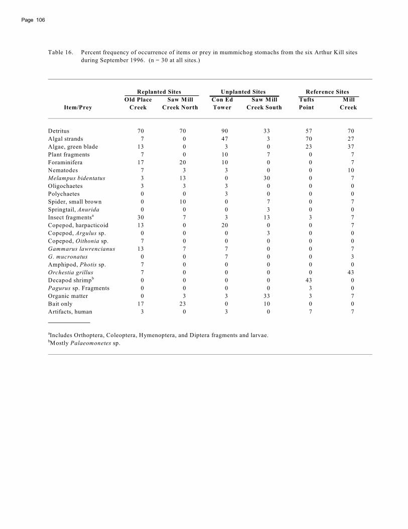
Page 106

Table 16. Percent frequency of occurrence of items or prey in mummichog stomachs from the six Arthur Kill sites

during September 1996. (n = 30 at all sites.)

Replanted Sites Unplanted Sites Reference Sites

Old Place Saw Mill Con Ed Saw Mill Tufts Mill

Item/Prey Creek Creek North Tower Creek South Point Creek

Detritus 70 70 90 33 57 70

Algal strands 7 0 47 3 70 27

Algae, green blade 13 0 3 0 23 37

Plant fragments 7 0 10 7 0 7

Foraminifera 17 20 10 0 0 7

Nematodes 7 3 3 0 0 10

Melampus bidentatus 3 13 0 30 0 7

Oligochaetes 3 3 3 0 0 0

Polychaetes 0 0 3 0 0 0

Spider, small brown 0 10 0 7 0 7

Springtail, Anurida 0 0 0 3 0 0

Insect fragments 30 7 3 13 3 7a

Copepod, harpacticoid 13 0 20 0 0 7

Copepod, Argulus sp. 0 0 0 3 0 0

Copepod, Oithonia sp. 7 0 0 0 0 0

Gammarus lawrencianus 13 7 7 0 0 7

G. mucronatus 0 0 7 0 0 3

Amphipod, Photis sp. 7 0 0 0 0 0

Orchestia grillus 7 0 0 0 0 43

Decapod shrimp 0 0 0 0 43 0b

Pagurus sp. Fragments 0 0 0 0 3 0

Organic matter 0 3 3 33 3 7

Bait only 17 23 0 10 0 0

Artifacts, human 3 0 3 0 7 7

Includes Orthoptera, Coleoptera, Hymenoptera, and Diptera fragments and larvae.a

Mostly Palaeomonetes sp.b

107Page

Table 17. Mean percent stomach volume estimates of items or prey in mummichog stomachs from the six Arthur Kill

sites during September 1996. (n = 30 at all sites.)

Replanted Sites Unplanted Sites Reference Sites

Old Place Saw Mill Con Ed Saw Mill Tufts Mill

Item/Prey Creek Creek North Tower Creek South Point Creek

Detritus 34.9 5 51 6.8 10 14.9

Algal strands <0.1 0 13 <0.1 36.8 11.8

Algae, green blade 4.1 0 0.3 0 11.8 16.8

Plant fragments <0.1 0 3.3 0.8 0 1

Foraminifera <0.1 <0.1 <0.1 0 0 <0.1

Nematodes <0.1 <0.1 <0.1 0 0 <0.1

Melampus bidentatus <0.1 <0.1 0 3.8 0 <0.1

Oligochaetes <0.1 <0.1 <0.1 0 0 0

Polychaetes 0 0 <0.1 0 0 0

Spider, small brown 0 <0.1 0 6.2 0 <0.1

Springtail, Anurida 0 0 0 <0.1 0 0

Insect fragments 0.4 <0.1 1 3 1.2 <0.1a

Copepod, harpacticoid <0.1 0 0.3 0 0 <0.1

Copepod, Argulus sp. 0 0 0 <0.1 0 0

Copepod, Oithonia sp. 0 0 0 <0.1 0 0

Gammarus lawrencianus 3.4 <0.1 0.2 0 0 3.3

G. mucronatus 0 0 3.7 0 0 <0.1

Amphipod, Photis sp. <0.1 0 0 0 0 0

Orchestia grillus 0 0 0 0 0 21.9

Decapod shrimp 0 0 0 0 26.8 0b

Pagurus sp. fragments 0 0 0 0 2.2 0

Organic matter 0 3.3 2.3 26.3 <0.1 2.3

Bait only 57.1 91.7 24.6 53.1 11.2 28

Artifacts, human <0.1 0 0.3 0 <0.1 <0.1

Includes Orthoptera, Coleoptera, Hymenoptera, and Diptera fragments and larvae.a

Mostly Palaeomonetes sp.b

Page 108

Table 18. Percent frequency of occurrence of items or prey in mummichog stomachs from the six Arthur Kill sites

during May-August 1997. (n = 30 at all sites.)

Replanted Sites Unplanted Sites Reference Sites

Old Place Saw Mill Con Ed Saw Mill Tufts Mill

Item/Prey Creek Creek North Tower Creek South Point Creek

Detritus 47 57 63 30 17 20

Algal strands 0 0 17 3 3 20

Algae, green blade 20 13 17 20 0 0

Plant fragments 7 7 17 0 3 7

Nematodes 7 7 17 20 13 23

Melampus bidentatus 3 0 0 0 0 3

Oligochaetes 0 0 3 0 0 0

Polychaetes 10 0 7 0 3 0a

Spider 0 0 3 0 0 0

Insect fragments 33 10 27 27 0 17b

Copepod, harpacticoid 0 0 0 0 50 0

Gammarus sp. 7 0 10 0 3 0

Amphipod fragments 70 33 50 53 17 47c

Decapod shrimp 0 0 3 0 0 0d

Organic matter 0 10 20 30 3 20

Fish eggs 0 0 0 0 0 13

Invertebrate eggs 3 0 3 3 0 57

Clam fragments 3 0 0 0 0 0

Cirolana 13 0 7 0 0 0

Crab fragments 0 0 7 0 0 0

Slug-like 0 3 0 0 27 0

Cyathura 0 3 0 3 0 3

Mostly Nereis succinea.a

Includes Orthoptera, Coleoptera, Hymenoptera, and Diptera fragments and larvae.b

Mostly Gammarus sp.c

Mostly Palaemonetes sp.d

109Page

Table 19. Mean percent stomach volume estimates of items or prey in mummichog stomachs from the six Arthur Kill

sites during May-August 1997. (n = 30 at all sites.)

Replanted Sites Unplanted Sites Reference Sites

Old Place Saw Mill Con Ed Saw Mill Tufts Mill

Item/Prey Creek Creek North Tower Creek South Point Creek

Detritus 20.3 43.4 39.1 24.0 13.9 14.1

Algal strands 0 0 9.2 0.2 0.4 2.7

Algae, green blade 8.8 8.7 2.7 3.8 0 0

Plant fragments 0.7 0.7 1.7 0 1.9 0.4

Nematodes 0.3 0.1 0.3 0.5 0.7 0.5

Melampus bidentatus 2.5 0 0 0 0 0.1

Oligochaetes 0 0 <0.1 0 0 0

Polychaetes 2.4 0 3.1 0 2.9 0a

Spider 0 0 <0.1 0 0 0

Insect fragments 8.3 1.8 3.6 8.2 0 2.0b

Copepod, harpacticoid 0 0 0 0 42.9 0

Gammarus sp. 2.5 0 1.0 0 3.8 0

Amphipod fragments 43.3 20.5 15.9 32.3 9.8 22.5c

Decapod shrimp 0 0 3.3 0 0 0d

Organic matter 0 6.0 9.4 23.8 0.8 8.2

Fish eggs 0 0 0 0 0 4.1

Invertebrate eggs <0.1 0 <0.1 <0.1 0 34.8

Clam fragments 0.8 0 0 0 0 0

Cirolana 6.5 0 0.5 0 0 0

Crab fragments 0 0 3.7 0 0 0

Slug-like 0 0.2 0 0 22.9 0

Cyathura 0 1.7 0 0.3 0 0.3

Mostly Nereis succinea.a

Includes Orthoptera, Coleoptera, Hymenoptera, and Diptera fragments and larvae.b

Mostly Gammarus sp.c

Mostly Palaemonetes sp.d

Page 110

111Page

VIII. CONCLUSIONS

Creek. This increased foraging success suggests that therewere greater numbers of prey (i.e., mummichogs) availableto the birds at the replanted site. Thus, the replanted siteappears to provide better foraging habitat for the wadingbirds. Supplementary data show that the heterogeneity ofthe habitat in the replanted marsh is positively correlatedwith improved foraging success.

These monitoring studies by the SMRT suggest thatthe replanting of S. alterniflora after the 1990 oil spill wasvery important for the recovery and restoration of thesaltmarsh ecosystem, especially at Old Place Creek, andeven in such a heavily urbanized and degraded estuary asthe Arthur Kill. The S. alterniflora provides much of thestructural component of the marsh; restoring this compo-nent is important to the other members of the food web,such as the mussels, mummichogs [e.g., as a refuge frompredation (Moy and Levin 1991; Halpin 2000)], and birds. Itis particularly important in an urbanized landscape wherehabitats are isolated and their availability is limited(Simenstad and Thom 1996; Ehrenfeld 2000), and where res-toration is critical for species of particular concern such asthe great and snowy egrets.

NMFS STUDY

Bearing in mind that the NMFS assessment was limitedin scope, our results are less clear in terms of the benefits ofreplanting, or even in evaluating the differences among thesites. Ehrenfeld (2000) stated that in urban wetlands, therange of variability, both within and among wetlands, ismuch higher than in nonurban wetlands, and this is cer-tainly true in the Arthur Kill. For example, for the benthicinfauna, while there may be similarities in invertebrate abun-dances between the replanted and reference sites, quanti-tative evaluation was confounded by the high variability inthe data and the low number of replanted and referencesites sampled. What is clear is that many of the faunafound in these marshes appear to be tolerant of contami-nants; however, this pollution and other anthropogenicimpacts may affect their overall health and longevity (e.g.,mummichogs). While it is true that the ribbed-mussels fromthe Mill Creek reference marsh grew faster and were largerand heavier than mussels from both replanted sites, this ismore likely due to the relative undisturbed nature of thismature marsh, as well as differences in site-specific factors.

All the Arthur Kill marshes are polluted of course, asevidenced by, for example, the residual oil in the sediments(see also Bergen et al. 2000), and as suggested by the highpercentages of detritus and algae as opposed to live prey inthe mummichog stomachs, which may indicate a poor dietdue to a polluted environment. However, the levels of con-taminants are often site specific, depending, for example, aswith sediment trace metals, on the types of sediment found

Before discussing the overall conclusions of the NMFSstudy, it is important to summarize the monitoring resultsand conclusions of the SMRT study for S. alterniflora bio-mass and stem densities, ribbed-mussel densities, mummi-chog abundances, and wading bird foraging success.

SMRT STUDY

The following summary of the SMRT study is based onBergen et al. (2000) and Alderson et al. (Salt Marsh Resto-ration Team, Natural Resources Group, New York City Parks,200 Nevada Ave., Staten Island, NY, pers. comm. and unpubl.data). No specific numbers will be given, and the results areconfined to Old Place Creek and Con Ed Tower. In terms ofS. alterniflora, above-ground biomass at Old Place Creek -- an oiled and replanted site -- has reached levels compa-rable to those reported in other studies at this latitude. Incomparison, little or no S. alterniflora has been found atCon Ed Tower -- an oiled and unplanted site; naturalrecolonization via rhizomatous growth and seedling recruit-ment has failed to re-establish vegetation there. At OldPlace Creek, annual increases in stem densities, and theheight of S. alternilfora plants, indicate that the conditionsfor seed dispersal and possible germination, as well as thebaffling and accretion of sediments, are being met at thatsite. The replanting of grass to areas at Old Place Creekdenuded by oil, and the subsequent success of the seed-lings and transplants, were not suggested by previous stud-ies; indeed, at the time of the spill, managers consideredreplanting unnecessary (C. Alderson et al., Salt Marsh Res-toration Team, Natural Resources Group, New York CityParks, 200 Nevada Ave., Staten Island, NY, pers. comm.). AtCon Ed Tower, though, the grass does not appear to be ableto return on its own, and a net loss of marsh greater thanthat caused by the oil spill may in fact be occurring due toerosion of the denuded shoreline (C. Alderson et al., SaltMarsh Restoration Team, Natural Resources Group, NewYork City Parks, 200 Nevada Ave., Staten Island, NY, pers.comm.).

Densities of mussels at Old Place Creek have increasedannually, while the mussels at Con Ed Tower are still at verylow densities.

Greater numbers of mummichogs were trapped at OldPlace Creek, suggesting a preference by that species for theheterogeneous habitat provided by the replanted S.alterniflora as compared to the bare surface of the Con EdTower site. Other studies have also shown greater directuse of salt marshes by fishes in comparison withnonvegetated habitat (e.g., Rozas and Minello 1998).

For snowy (Egretta thula) and great egrets(Casmerodius albus), the number and duration of foragingvisits, the number of strike attempts, and the number ofsuccessful strikes were significantly greater at Old Place

Page 112

at each site. Replanting may have reduced the amount ofTPH in the sediments -- compare Old Place Creek to Con EdTower, and see also Bergen et al. (2000); however, replant-ing may not have had a great effect on the levels of othercontaminants, such as trace metals in both sediments andmussels, and TPH in mussels.

Some measures of ecological function, such as bio-geochemistry, also appear to be site specific, but are sub-ject to many confounding factors, and it is questionablewhether the biogeochemistry was affected by replanting.Others measures, such as mummichog food habits, may ormay not be site specific, but a more thorough investigationwould be necessary to discern any real patterns in the data,as has been demonstrated for several of our other investi-gations.

COMBINED STUDIES

In conclusion, replanting the oil-damaged marshes ofthe Arthur Kill may have successfully “restored” them, atleast structurally, to the level of the existing marshes foundwithin the Kill. Because this is an urban estuary, the extentto which the ecological functions of these marshes havebeen restored is more difficult to ascertain due to confound-ing factors such as pollution and other anthropogenic im-pacts.

Also, the time span of this preliminary assessment pro-gram may have been too short and the number of treatmentsites chosen may have been too small to assess accuratelythe performance of the replanted marshes, especially giventhe many scales of natural spatial and temporal variabilityand anthropogenic perturbations inherent in this ecosys-tem. A number of habitat restoration investigators havealso noted the value and importance of long-term studies ofecosystem processes in restoration research in order to

obtain a better understanding of the time required to achievefunctional equivalency and to also take into account thiskind of variability (e.g., Simenstad and Thom 1996; Kentula2000; West et al. 2000). Nevertheless, New York City’s SMRTcontinues to replant and monitor these marshes where nec-essary, insuring that this vital habitat is protected from fur-ther loss and degradation.

REFERENCES CITED

Bergen, A.; Alderson, C.; Bergfors, R.; Aquila, C.; Matsil, M.A.2000. Restoration of a Spartina alterniflora salt marshfollowing a fuel oil spill, New York City, NY. WetlandsEcol. Manage. 8:185-195.

Ehrenfeld, J.G. 2000. Evaluating wetlands within an urbancontext. Ecol. Eng. 15:253-265.

Halpin, P.M. 2000. Habitat use by an intertidal salt-marsh fish:trade-offs between predation and growth. Mar. Ecol. Prog.Ser. 198:203-214.

Kentula, M.E. 2000. Perspectives on setting success criteriafor wetland restoration. Ecol. Eng. 15:199-209.

Moy, L.D.; Levin, L.A. 1991. Are Spartina marshes a replace-able resource? A functional approach to evaluation ofmarsh creation efforts. Estuaries 14:1-16.

Rozas, L.P.; Minello, T.J. 1998. Nekton use of salt marsh,seagrass, and nonvegetated habitats in a south Texas(USA) estuary. Bull. Mar. Sci. 63:481-501.

Simenstad, C.A.; Thom, R.M. 1996. Functional equivalencytrajectories of the restored Gog-Le-Hi-Te estuarine wet-land. Ecol. Appl. 6:38-56.

West, T.L.; Cough, L.M.; Ambrose, W.G., Jr. 2000. Assessmentof function in an oligohaline environment: lessons learnedby comparing created and natural habitats. Ecol. Eng.15:303-321.

113Page

ACKNOWLEDGMENTS

NMFS funding was provided by the NMFS Office of Habitat Conservation/Restoration Center. The authors wouldparticularly like to express their appreciation to New York City’s Salt Marsh Restoration Team: Carl Alderson, AndrewBergen, Robbin Bergfors, and others from that office who helped us with the study and allowed us access to theirrestoration sites.

We thank Beth Leimburg and others for help in the field with sampling of ribbed-mussels during the age, growth, andallometric relationships phase of this study. We greatly appreciate the work of Vickie Bejda and her students in theAdvanced Biology Class at Ocean Township High School, Ocean Township, New Jersey, for doing the weight and lengthmeasurements and compiling those data. We also thank Bob Reid and Anthony Paulson for helpful comments on earlierdrafts of the chapter on age, growth, and allometric relationships of ribbed-mussels.

We thank Andrew Draxler for help with sampling the benthic invertebrates, and Fred Triolo for sorting most of thosesamples.

Page 114

115Page

APPENDIX A

PRINCIPAL COMPONENT ANALYSIS OF TRACE METALS

Table A1. Eigenvectors for trace metals and organic carbon content in sediments from the September 1996 and May 1997collections, excluding the Sandy Hook site

Table A2. Eigenvectors for trace metals and % fines in sediments from the September 1996 collection, excluding the ConEd Tower site

Table A3. Eigenvectors for trace metals in ribbed-mussels from the September 1996 and May 1997 collections

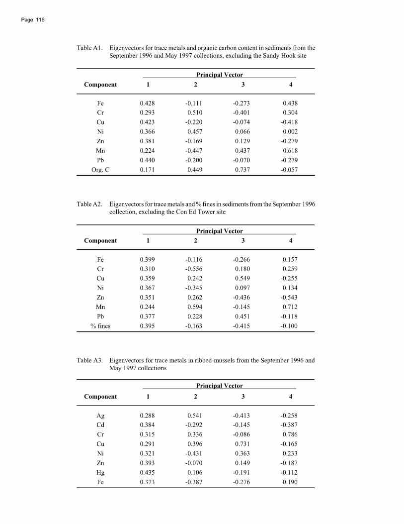
Table A1. Eigenvectors for trace metals and organic carbon content in sediments from theSeptember 1996 and May 1997 collections, excluding the Sandy Hook site

Principal Vector Component 1 2 3 4

Fe 0.428 -0.111 -0.273 0.438Cr 0.293 0.510 -0.401 0.304Cu 0.423 -0.220 -0.074 -0.418Ni 0.366 0.457 0.066 0.002Zn 0.381 -0.169 0.129 -0.279Mn 0.224 -0.447 0.437 0.618Pb 0.440 -0.200 -0.070 -0.279

Org. C 0.171 0.449 0.737 -0.057

Table A2. Eigenvectors for trace metals and % fines in sediments from the September 1996collection, excluding the Con Ed Tower site

Principal Vector Component 1 2 3 4

Fe 0.399 -0.116 -0.266 0.157Cr 0.310 -0.556 0.180 0.259Cu 0.359 0.242 0.549 -0.255Ni 0.367 -0.345 0.097 0.134Zn 0.351 0.262 -0.436 -0.543Mn 0.244 0.594 -0.145 0.712Pb 0.377 0.228 0.451 -0.118

% fines 0.395 -0.163 -0.415 -0.100

Table A3. Eigenvectors for trace metals in ribbed-mussels from the September 1996 andMay 1997 collections

Principal Vector Component 1 2 3 4

Ag 0.288 0.541 -0.413 -0.258Cd 0.384 -0.292 -0.145 -0.387Cr 0.315 0.336 -0.086 0.786Cu 0.291 0.396 0.731 -0.165Ni 0.321 -0.431 0.363 0.233Zn 0.393 -0.070 0.149 -0.187Hg 0.435 0.106 -0.191 -0.112Fe 0.373 -0.387 -0.276 0.190

Page 116

117Page

APPENDIX B

SAMPLE CHARACTERISTICS FOR ANALYSIS OF PETROLEUM HYDROCARBONS

Table B1. The location and collection dates for sediment and ribbed mussels from the Arthur Kill and Sandy Hook BayTable B2. Date of collection, physical parameters, and percent lipid for analyzed ribbed musselsTable B3. Members of each batch for cleanup and analysis of Arthur Kill sedimentsTable B4. Members of each batch for cleanup and analysis of Arthur Kill musselsTable B5. Aliphatic hydrocarbons analyzed

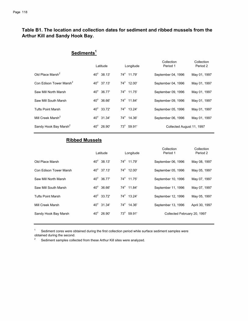
Table B1. The location and collection dates for sediment and ribbed mussels from the Arthur Kill and Sandy Hook Bay.

Sediments1

Latitude LongitudeCollectionPeriod 1

CollectionPeriod 2

Old Place Marsh2 40o 38.13' 74o 11.79' September 04, 1996 May 01, 1997

Con Edison Tower Marsh2 40o 37.13' 74o 12.00' September 04, 1996 May 01, 1997

Saw Mill North Marsh 40o 36.77' 74o 11.75' September 09, 1996 May 01, 1997

Saw Mill South Marsh 40o 36.66' 74o 11.84' September 09, 1996 May 01, 1997

Tufts Point Marsh 40o 33.72' 74o 13.24' September 05, 1996 May 01, 1997

Mill Creek Marsh2 40o 31.34' 74o 14.36' September 06, 1996 May 01, 1997

Sandy Hook Bay Marsh2 40o 26.90' 73o 59.91' Collected August 11, 1997

Ribbed Mussels

Latitude LongitudeCollectionPeriod 1

CollectionPeriod 2

Old Place Marsh 40o 38.13' 74o 11.79' September 06, 1996 May 08, 1997

Con Edison Tower Marsh 40o 37.13' 74o 12.00' September 05, 1996 May 05, 1997

Saw Mill North Marsh 40o 36.77' 74o 11.75' September 10, 1996 May 07, 1997

Saw Mill South Marsh 40o 36.66' 74o 11.84' September 11, 1996 May 07, 1997

Tufts Point Marsh 40o 33.72' 74o 13.24' September 12, 1996 May 05, 1997

Mill Creek Marsh 40o 31.34' 74o 14.36' September 13, 1996 April 30, 1997

Sandy Hook Bay Marsh 40o 26.90' 73o 59.91' Collected February 20, 1997

1 Sediment cores were obtained during the first collection period while surface sediment samples were obtained during the second.2 Sediment samples collected from these Arthur Kill sites were analyzed.

Page 118

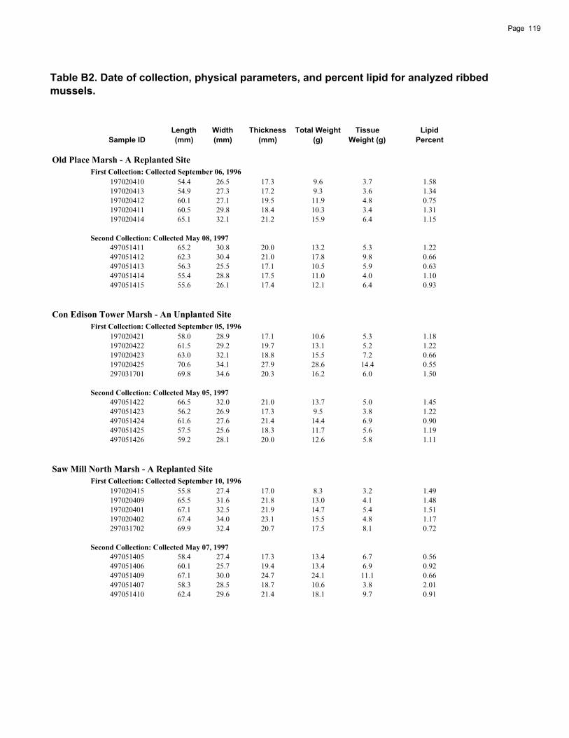
Table B2. Date of collection, physical parameters, and percent lipid for analyzed ribbed mussels.

Sample IDLength(mm)

Width(mm)

Thickness(mm)

Total Weight (g)

TissueWeight (g)

LipidPercent

Old Place Marsh - A Replanted Site First Collection: Collected September 06, 1996

197020410 54.4 26.5 17.3 9.6 3.7 1.58197020413 54.9 27.3 17.2 9.3 3.6 1.34197020412 60.1 27.1 19.5 11.9 4.8 0.75197020411 60.5 29.8 18.4 10.3 3.4 1.31197020414 65.1 32.1 21.2 15.9 6.4 1.15

Second Collection: Collected May 08, 1997497051411 65.2 30.8 20.0 13.2 5.3 1.22497051412 62.3 30.4 21.0 17.8 9.8 0.66497051413 56.3 25.5 17.1 10.5 5.9 0.63497051414 55.4 28.8 17.5 11.0 4.0 1.10497051415 55.6 26.1 17.4 12.1 6.4 0.93

Con Edison Tower Marsh - An Unplanted Site First Collection: Collected September 05, 1996

197020421 58.0 28.9 17.1 10.6 5.3 1.18197020422 61.5 29.2 19.7 13.1 5.2 1.22197020423 63.0 32.1 18.8 15.5 7.2 0.66197020425 70.6 34.1 27.9 28.6 14.4 0.55297031701 69.8 34.6 20.3 16.2 6.0 1.50

Second Collection: Collected May 05, 1997497051422 66.5 32.0 21.0 13.7 5.0 1.45497051423 56.2 26.9 17.3 9.5 3.8 1.22497051424 61.6 27.6 21.4 14.4 6.9 0.90497051425 57.5 25.6 18.3 11.7 5.6 1.19497051426 59.2 28.1 20.0 12.6 5.8 1.11

Saw Mill North Marsh - A Replanted Site First Collection: Collected September 10, 1996

197020415 55.8 27.4 17.0 8.3 3.2 1.49197020409 65.5 31.6 21.8 13.0 4.1 1.48197020401 67.1 32.5 21.9 14.7 5.4 1.51197020402 67.4 34.0 23.1 15.5 4.8 1.17297031702 69.9 32.4 20.7 17.5 8.1 0.72

Second Collection: Collected May 07, 1997497051405 58.4 27.4 17.3 13.4 6.7 0.56497051406 60.1 25.7 19.4 13.4 6.9 0.92497051409 67.1 30.0 24.7 24.1 11.1 0.66497051407 58.3 28.5 18.7 10.6 3.8 2.01497051410 62.4 29.6 21.4 18.1 9.7 0.91

119Page

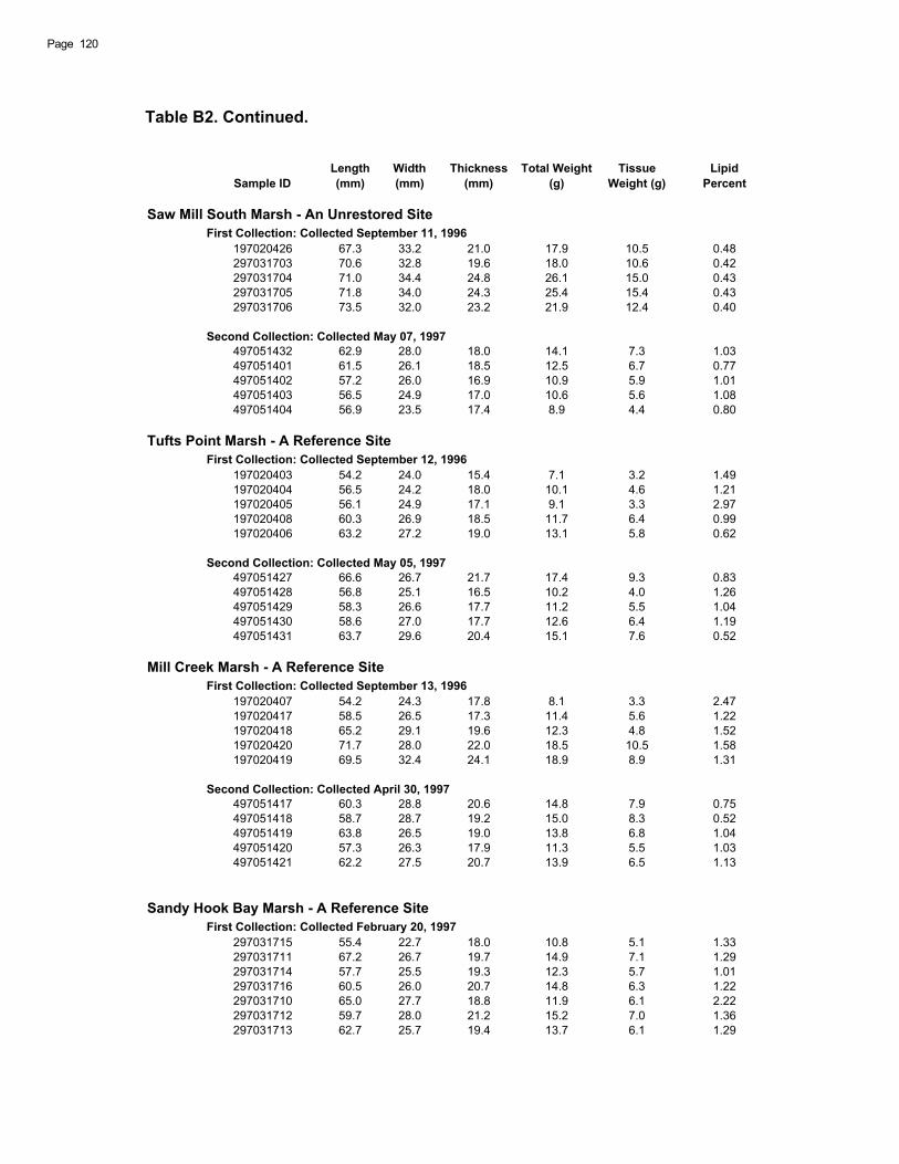
Table B2. Continued.

Sample IDLength(mm)

Width(mm)

Thickness(mm)

Total Weight (g)

TissueWeight (g)

LipidPercent

Saw Mill South Marsh - An Unrestored Site First Collection: Collected September 11, 1996

197020426 67.3 33.2 21.0 17.9 10.5 0.48297031703 70.6 32.8 19.6 18.0 10.6 0.42297031704 71.0 34.4 24.8 26.1 15.0 0.43297031705 71.8 34.0 24.3 25.4 15.4 0.43297031706 73.5 32.0 23.2 21.9 12.4 0.40

Second Collection: Collected May 07, 1997497051432 62.9 28.0 18.0 14.1 7.3 1.03497051401 61.5 26.1 18.5 12.5 6.7 0.77497051402 57.2 26.0 16.9 10.9 5.9 1.01497051403 56.5 24.9 17.0 10.6 5.6 1.08497051404 56.9 23.5 17.4 8.9 4.4 0.80

Tufts Point Marsh - A Reference Site First Collection: Collected September 12, 1996

197020403 54.2 24.0 15.4 7.1 3.2 1.49197020404 56.5 24.2 18.0 10.1 4.6 1.21197020405 56.1 24.9 17.1 9.1 3.3 2.97197020408 60.3 26.9 18.5 11.7 6.4 0.99197020406 63.2 27.2 19.0 13.1 5.8 0.62

Second Collection: Collected May 05, 1997497051427 66.6 26.7 21.7 17.4 9.3 0.83497051428 56.8 25.1 16.5 10.2 4.0 1.26497051429 58.3 26.6 17.7 11.2 5.5 1.04497051430 58.6 27.0 17.7 12.6 6.4 1.19497051431 63.7 29.6 20.4 15.1 7.6 0.52

Mill Creek Marsh - A Reference Site First Collection: Collected September 13, 1996

197020407 54.2 24.3 17.8 8.1 3.3 2.47197020417 58.5 26.5 17.3 11.4 5.6 1.22197020418 65.2 29.1 19.6 12.3 4.8 1.52197020420 71.7 28.0 22.0 18.5 10.5 1.58197020419 69.5 32.4 24.1 18.9 8.9 1.31

Second Collection: Collected April 30, 1997497051417 60.3 28.8 20.6 14.8 7.9 0.75497051418 58.7 28.7 19.2 15.0 8.3 0.52497051419 63.8 26.5 19.0 13.8 6.8 1.04497051420 57.3 26.3 17.9 11.3 5.5 1.03497051421 62.2 27.5 20.7 13.9 6.5 1.13

Sandy Hook Bay Marsh - A Reference Site First Collection: Collected February 20, 1997

297031715 55.4 22.7 18.0 10.8 5.1 1.33297031711 67.2 26.7 19.7 14.9 7.1 1.29297031714 57.7 25.5 19.3 12.3 5.7 1.01297031716 60.5 26.0 20.7 14.8 6.3 1.22297031710 65.0 27.7 18.8 11.9 6.1 2.22297031712 59.7 28.0 21.2 15.2 7.0 1.36297031713 62.7 25.7 19.4 13.7 6.1 1.29

Page 120

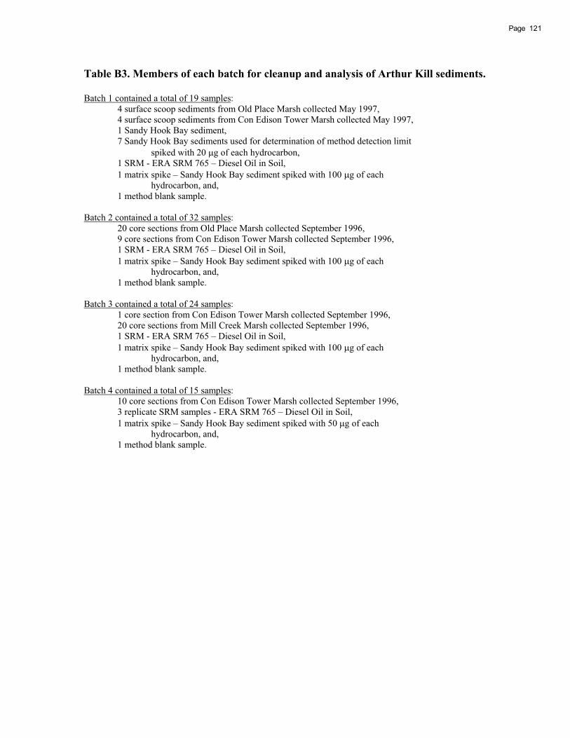
Table B3. Members of each batch for cleanup and analysis of Arthur Kill sediments.

Batch 1 contained a total of 19 samples: 4 surface scoop sediments from Old Place Marsh collected May 1997, 4 surface scoop sediments from Con Edison Tower Marsh collected May 1997, 1 Sandy Hook Bay sediment, 7 Sandy Hook Bay sediments used for determination of method detection limit

spiked with 20 g of each hydrocarbon, 1 SRM - ERA SRM 765 – Diesel Oil in Soil, 1 matrix spike – Sandy Hook Bay sediment spiked with 100 g of each

hydrocarbon, and, 1 method blank sample.

Batch 2 contained a total of 32 samples: 20 core sections from Old Place Marsh collected September 1996, 9 core sections from Con Edison Tower Marsh collected September 1996,

1 SRM - ERA SRM 765 – Diesel Oil in Soil, 1 matrix spike – Sandy Hook Bay sediment spiked with 100 g of each hydrocarbon, and, 1 method blank sample.

Batch 3 contained a total of 24 samples: 1 core section from Con Edison Tower Marsh collected September 1996, 20 core sections from Mill Creek Marsh collected September 1996,

1 SRM - ERA SRM 765 – Diesel Oil in Soil, 1 matrix spike – Sandy Hook Bay sediment spiked with 100 g of each hydrocarbon, and, 1 method blank sample.

Batch 4 contained a total of 15 samples: 10 core sections from Con Edison Tower Marsh collected September 1996, 3 replicate SRM samples - ERA SRM 765 – Diesel Oil in Soil,

1 matrix spike – Sandy Hook Bay sediment spiked with 50 g of each hydrocarbon, and, 1 method blank sample.

121Page

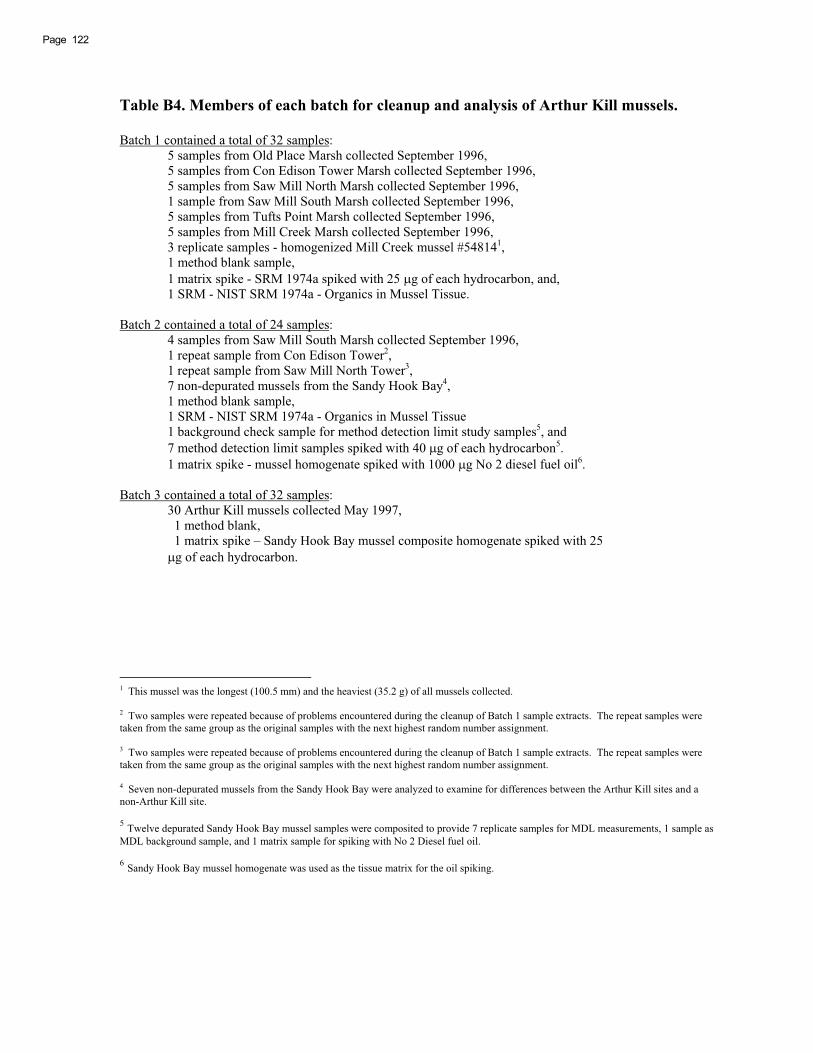
Table B4. Members of each batch for cleanup and analysis of Arthur Kill mussels.

Batch 1 contained a total of 32 samples: 5 samples from Old Place Marsh collected September 1996, 5 samples from Con Edison Tower Marsh collected September 1996, 5 samples from Saw Mill North Marsh collected September 1996, 1 sample from Saw Mill South Marsh collected September 1996, 5 samples from Tufts Point Marsh collected September 1996, 5 samples from Mill Creek Marsh collected September 1996, 3 replicate samples - homogenized Mill Creek mussel #548141, 1 method blank sample, 1 matrix spike - SRM 1974a spiked with 25 g of each hydrocarbon, and, 1 SRM - NIST SRM 1974a - Organics in Mussel Tissue.

Batch 2 contained a total of 24 samples: 4 samples from Saw Mill South Marsh collected September 1996, 1 repeat sample from Con Edison Tower2, 1 repeat sample from Saw Mill North Tower3, 7 non-depurated mussels from the Sandy Hook Bay4, 1 method blank sample, 1 SRM - NIST SRM 1974a - Organics in Mussel Tissue 1 background check sample for method detection limit study samples5, and 7 method detection limit samples spiked with 40 g of each hydrocarbon5. 1 matrix spike - mussel homogenate spiked with 1000 g No 2 diesel fuel oil6.

Batch 3 contained a total of 32 samples: 30 Arthur Kill mussels collected May 1997, 1 method blank, 1 matrix spike – Sandy Hook Bay mussel composite homogenate spiked with 25

g of each hydrocarbon.

1 This mussel was the longest (100.5 mm) and the heaviest (35.2 g) of all mussels collected.

2 Two samples were repeated because of problems encountered during the cleanup of Batch 1 sample extracts. The repeat samples were taken from the same group as the original samples with the next highest random number assignment.

3 Two samples were repeated because of problems encountered during the cleanup of Batch 1 sample extracts. The repeat samples were taken from the same group as the original samples with the next highest random number assignment.

4 Seven non-depurated mussels from the Sandy Hook Bay were analyzed to examine for differences between the Arthur Kill sites and a non-Arthur Kill site.

5 Twelve depurated Sandy Hook Bay mussel samples were composited to provide 7 replicate samples for MDL measurements, 1 sample asMDL background sample, and 1 matrix sample for spiking with No 2 Diesel fuel oil.

6 Sandy Hook Bay mussel homogenate was used as the tissue matrix for the oil spiking.

Page 122

Table B5. Aliphatic hydrocarbons analyzed.

Chemical Name Abbreviation

Normal Aliphatic Hydrocarbons

n-Octane1 n-C8 n-Nonane n-C9 n-Decane n-C10 n-Undecane n-C11 n-Dodecane n-C12 n-Tridecane n-C13 n-Tetradecane n-C14 n-Pentadecane n-C15

n-Hexadecane n-C16n-Heptadecane n-C17n-Octadecane n-C18n-Nonadecane n-C19n-Eicosane n-C20n-Heneicosane n-C21n-Docosane n-C22n-Tricosane n-C23n-Tetracosane n-C24n-Pentacosane n-C25n-Hexacosane n-C26

n-Heptacosane n-C27 n-Octacosane n-C28

n-Nonacosane n-C29 n-Triacontane n-C30 n-Hentriacontane n-C31 n-Dotriacontane n-C32 n-Tritriacontane n-C33

n-Tetratriacontane n-C34 n-Pentatriacontane n-C35 n-Hexatriacontane n-C36 n-Heptatriacontane n-C37 n-Octatriacontane n-C38

n-Nonatriacontane n-C39 n-Tetracontane n-C40

Branched Aliphatic Hydrocarbons

2,6,10,14-Tetramethylhexadecane Pristane 2,6,10,14-Tetramethylpentadecane Phytane

1 The concentrations for n-C8 will be not reported, since it was difficult to identify this peak in samples and to determine MDL for n-C8.

123Page

Page 124

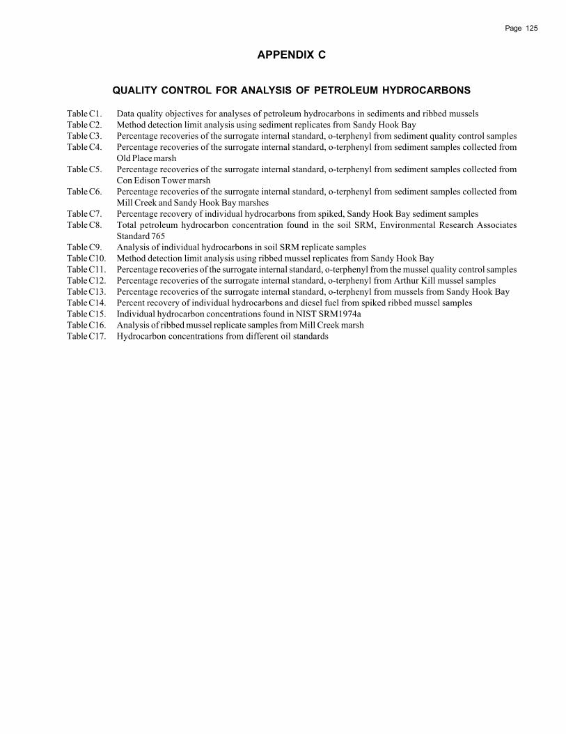
125Page

APPENDIX C

QUALITY CONTROL FOR ANALYSIS OF PETROLEUM HYDROCARBONS

Table C1. Data quality objectives for analyses of petroleum hydrocarbons in sediments and ribbed musselsTable C2. Method detection limit analysis using sediment replicates from Sandy Hook BayTable C3. Percentage recoveries of the surrogate internal standard, o-terphenyl from sediment quality control samplesTable C4. Percentage recoveries of the surrogate internal standard, o-terphenyl from sediment samples collected from

Old Place marshTable C5. Percentage recoveries of the surrogate internal standard, o-terphenyl from sediment samples collected from

Con Edison Tower marshTable C6. Percentage recoveries of the surrogate internal standard, o-terphenyl from sediment samples collected from

Mill Creek and Sandy Hook Bay marshesTable C7. Percentage recovery of individual hydrocarbons from spiked, Sandy Hook Bay sediment samplesTable C8. Total petroleum hydrocarbon concentration found in the soil SRM, Environmental Research Associates

Standard 765Table C9. Analysis of individual hydrocarbons in soil SRM replicate samplesTable C10. Method detection limit analysis using ribbed mussel replicates from Sandy Hook BayTable C11. Percentage recoveries of the surrogate internal standard, o-terphenyl from the mussel quality control samplesTable C12. Percentage recoveries of the surrogate internal standard, o-terphenyl from Arthur Kill mussel samplesTable C13. Percentage recoveries of the surrogate internal standard, o-terphenyl from mussels from Sandy Hook BayTable C14. Percent recovery of individual hydrocarbons and diesel fuel from spiked ribbed mussel samplesTable C15. Individual hydrocarbon concentrations found in NIST SRM1974aTable C16. Analysis of ribbed mussel replicate samples from Mill Creek marshTable C17. Hydrocarbon concentrations from different oil standards

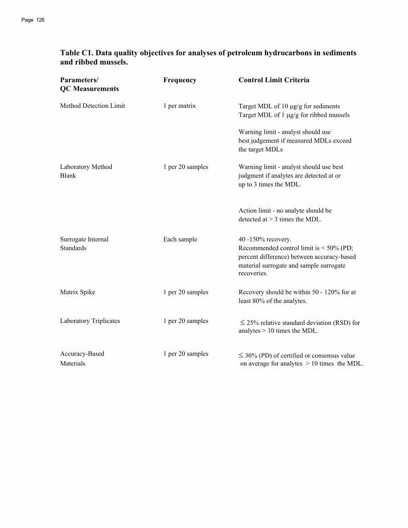
Table C1. Data quality objectives for analyses of petroleum hydrocarbons in sediments and ribbed mussels.

Parameters/ Frequency Control Limit Criteria QC Measurements

Method Detection Limit 1 per matrix Target MDL of 10 g/g for sediments Target MDL of 1 g/g for ribbed mussels

Warning limit - analyst should use best judgement if measured MDLs exceed the target MDLs

Laboratory Method 1 per 20 samples Warning limit - analyst should use best Blank judgment if analytes are detected at or

up to 3 times the MDL.

Action limit - no analyte should be detected at > 3 times the MDL.

Surrogate Internal Each sample 40 -150% recovery. Standards Recommended control limit is < 50% (PD;

percent difference) between accuracy-based material surrogate and sample surrogate

recoveries.

Matrix Spike 1 per 20 samples Recovery should be within 50 - 120% for at least 80% of the analytes.

Laboratory Triplicates 1 per 20 samples 25% relative standard deviation (RSD) for analytes > 10 times the MDL.

Accuracy-Based 1 per 20 samples 30% (PD) of certified or consensus value Materials on average for analytes > 10 times the MDL.

Page 126

127Page

Tabl

e C

2. M

etho

d D

etec

tion

Lim

it (M

DL)

ana

lysi

s us

ing

sedi

men

t rep

licat

es fr

om S

andy

Hoo

k B

ay.1

Sample ID

Nonane (n-C9)

Decane (n-C10)

Undecane (n-C11)

Dodecane (n-C12)

Tridecane (n-C13)

Tetradecane (n-C14)

Pentadecane (n-C15)

Hexadecane (n-C16)

Heptadecane (n-C17)

Pristane

Octadecane (n-C18)

Phytane

Nonadecane (n-C19)

Eicosane (n-C20)

Heneicosane (n-C21)

Docosane (n-C22)

Tricosane (n-C23)

Sedi

men

t M

DL

Det

erm

inat

ion

Usi

ng E

xter

nal S

tand

ard

Cal

cula

tions

(�g/

g, w

et w

t.)

8970

8110

92.

954.

234.

524.

574.

694.

965.

055.

295.

875.

385.

905.

616.

035.

936.

167.

206.

6889

7081

110

4.31

3.78

4.39

4.69

4.63

4.92

4.94

4.90

5.32

4.94

5.07

4.96

5.29

5.22

5.30

5.39

5.44

8970

8111

12.

593.

293.

904.

274.

344.

604.

875.

085.

635.

225.

595.

335.

695.

555.

836.

896.

1889

7081

112

3.36

3.24

3.70

4.01

4.07

4.23

4.58

4.69

5.19

4.81

5.00

4.90

5.26

5.16

5.31

5.28

5.40

8970

8111

33.

243.

244.

204.

594.

845.

155.

675.

806.

355.

906.

095.

946.

336.

336.

526.

606.

8389

7081

114

1.61

2.16

2.59

2.89

3.05

3.36

3.95

4.40

5.12

4.77

5.22

5.02

5.42

5.40

5.57

5.65

5.82

8970

8111

53.

093.

363.

423.

663.

824.

064.

334.

515.

084.

705.

114.

885.

365.

325.

505.

465.

62

Ave

rage

3.02

3.33

3.82

4.10

4.21

4.47

4.77

4.95

5.51

5.10

5.43

5.23

5.63

5.56

5.74

6.07

6.00

Std

Dev

0.82

0.63

0.67

0.64

0.63

0.63

0.55

0.49

0.47

0.43

0.44

0.41

0.41

0.43

0.46

0.80

0.58

%R

SD

or %

CV

27.0

619

.02

17.4

615

.73

14.8

814

.07

11.5

69.

868.

538.

398.

037.

827.

337.

677.

9913

.20

9.74

MD

L22.

571.

992.

092.

031.

971.

981.

731.

531.

481.

351.

371.

291.

301.

341.

442.

521.

84

1

The

sedi

men

t was

col

lect

ed fr

om H

orse

shoe

Cov

e, S

andy

Hoo

k. T

he s

edim

ent w

as th

en m

ixed

into

a c

ompo

site

and

por

tions

of t

his

com

posi

te w

as u

sed

for t

he M

DL

anal

ysis

. Eac

h sa

mpl

e w

asw

ith 2

0 �g

of e

ach

indi

vidu

al h

ydro

carb

on.

2 M

DL

= �t

; whe

re �

is th

e st

anda

rd d

evia

tion

and

t is

the

Stu

dent

s t v

alue

. For

99%

con

fiden

ce le

vel,

6 de

gree

s of

free

dom

(one

-taile

d), t

= 3

.143

.

Page 128

Tabl

e C

2. C

ontin

ued.

Sample ID

Tetracosane (n-C24)

Pentacosane (n-C25)

Hexacosane (n-C26)

Heptacosane (n-C27)

Octacosane (n-C28)

Nonacosane (n-C29)

Triacontane (n-C30)

n-Hentriacontane (n-C31)

Dotriacontane (n-C32)

Tritriacontane (n-C33)

Tetratriacontane (n-C34)

Pentatriacontane (n-C35)

Hexatriacontane (n-C36)

Heptatriacontane (n-C37)

Octatriacontane (n-C38)

Nonatriacontane (n-C39)

Tetracontane (n-C40)

Total Petroleum Hydrocarbons2

Sedi

men

t M

DL

Det

erm

inat

ion

Usi

ng E

xter

nal S

tand

ard

Cal

cula

tions

(�g/

g, w

et w

t.)

8970

8110

96.

196.

686.

087.

466.

5312

.39

5.79

9.01

5.21

8.07

2.33

2.40

1.30

1.04

0.84

0.71

0.60

4

64

8970

8111

05.

335.

775.

366.

335.

3910

.89

5.29

8.79

5.63

4.17

2.55

2.58

1.45

1.33

1.08

0.92

0.81

3

61

8970

8111

15.

826.

325.

606.

885.

8912

.37

5.70

8.40

4.78

6.35

3.05

3.46

1.77

1.61

1.39

1.20

1.08

3

40

8970

8111

25.

265.

645.

146.

345.

5611

.97

5.46

9.00

5.27

3.68

2.56

2.27

1.68

1.26

1.08

0.92

0.79

3

41

8970

8111

36.

497.

046.

327.

926.

0713

.63

6.16

10.2

25.

8610

.76

2.68

2.34

1.80

1.50

1.17

1.01

0.91

3

89

8970

8111

45.

535.

835.

366.

495.

0611

.13

5.20

8.21

4.36

5.24

2.45

2.56

1.22

1.03

0.82

0.71

0.56

2

81

8970

8111

55.

415.

795.

286.

455.

6910

.97

5.40

8.82

5.43

3.77

2.65

2.56

1.65

1.26

1.05

0.90

0.76

3

23

Ave

rage

5.72

6.15

5.59

6.84

5.74

11.9

15.

578.

925.

226.

002.

612.

591.

551.

291.

060.

910.

79

357

S

td D

ev0.

470.

540.

440.

620.

481.

000.

330.

650.

512.

620.

230.

400.

230.

220.

190.

170.

18

57.

6 %

RS

D o

r %C

V8.

208.

737.

929.

128.

358.

366.

017.

249.

7743

.70

8.66

15.3

714

.93

16.7

418

.28

18.6

022

.78

1

6.2

MD

L11.

471.

691.

391.

961.

513.

131.

052.

031.

608.

250.

711.

250.

730.

680.

610.

530.

56

181

1

MD

L = �t

; whe

re �

is th

e st

anda

rd d

evia

tion

and

t is

the

Stu

dent

s t v

alue

. For

99%

con

fiden

ce le

vel,

6 de

gree

s of

free

dom

(one

-taile

d), t

= 3

.143

.2

D

eter

min

ed fr

om th

e to

tal p

eak

area

s in

the

chro

mat

ogra

m fr

om n

-C8 t

o n-

C40

min

us a

ny c

ontri

butio

ns fr

om th

e in

tern

al s

tand

ard

area

s.

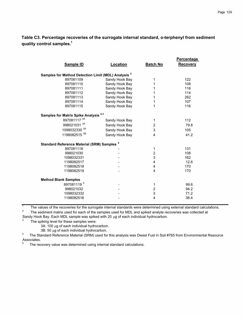
Table C3. Percentage recoveries of the surrogate internal standard, o-terphenyl from sediment quality control samples.1

Sample ID Location Batch NoPercentageRecovery

Samples for Method Detection Limit (MDL) Analysis 2

897081109 Sandy Hook Bay 1 122 897081110 Sandy Hook Bay 1 108 897081111 Sandy Hook Bay 1 116 897081112 Sandy Hook Bay 1 114 897081113 Sandy Hook Bay 1 262 897081114 Sandy Hook Bay 1 107 897081115 Sandy Hook Bay 1 116

Samples for Matrix Spike Analysis 2,3

897081117 3A Sandy Hook Bay 1 112 998021031 3A Sandy Hook Bay 2 79.8

1098032330 3A Sandy Hook Bay 3 105 1198082515 3B Sandy Hook Bay 4 41.2

Standard Reference Material (SRM) Samples 4

897081118 - 1 131 998021030 - 2 108

1098032331 - 3 162 1198082517 - 4 12.6 1198082518 - 4 170 1198082519 - 4 170

Method Blank Samples 897081119 5 - 1 99.6 998021032 - 2 94.2

1098032332 - 3 71.2 1198082516 - 4 36.4

1 The values of the recoveries for the surrogate internal standards were determined using external standard calculations. 2 The sediment matrix used for each of the samples used for MDL and spiked analyte recoveries was collected atSandy Hook Bay. Each MDL sample was spiked with 20 g of each individual hydrocarbon.3 The spiking level for these samples were:

3A: 100 g of each individual hydrocarbon.3B: 50 g of each individual hydrocarbon.

4 The Standard Reference Material (SRM) used for this analysis was Diesel Fuel in Soil #765 from Environmental ResourceAssociates.5 The recovery value was determined using internal standard calculations.

129Page

Table C4. Percentage recoveries of the surrogate internal standard, o-terphenyl from sediment samples collected from Old Place marsh.1

Sample ID Batch No Station Section No 2PercentageRecovery

September 1996 Collection998021001 2 A 1 88.4 998021002 2 A 2 95.2 998021003 2 A 3 106 998021004 2 A 4 80.8 998021005 2 A 5 741 998021006 2 B 1 158 998021007 2 B 2 218 998021008 2 B 3 189 998021009 2 B 4 206 998021010 2 B 5 173 998021011 2 C 1 130 998021012 2 C 2 133 998021013 2 C 3 110 998021014 2 C 4 118 998021015 2 C 5 118 998021016 2 D 1 138 998021017 2 D 2 120 998021018 2 D 3 168 998021019 2 D 4 130 998021020 2 D 5 599

May 1997 Collection897081101 1 A SC 104 897081102 1 B SC 53.7 897081103 1 C SC 120 897081104 1 D SC 105

1 The values of the recoveries for the surrogate internal standards were determined using external standard calculations. 2 The meaning of the Section No is:

1: Core section with depth 0 to 1 cm.2: Core section with depth 1 to 2 cm.3: Core section with depth 2 to 3 cm.4: Core section with depth 3 to 4 cm.5: Core section with depth 4 to 5 cm.SC: Surface Scoop.

Page 130

Table C5. Percentage recoveries of the surrogate internal standard, o-terphenyl from sediment samples collected from Con Edison Tower marsh.1

Sample ID Batch No Station Section No 2PercentageRecovery

September 1996 Collection998021021 2 A 1 980 998021022 2 A 2 1690 998021023 2 A 3 965 998021024 2 A 4 724 998021025 2 A 5 1050 998021026 2 B 1 1150 998021027 2 B 2 2490 998021028 2 B 3 6510 998021029 2 B 4 9900

1098032325 3 B 5 224 1198082510 4 C 1 208 1198082511 4 C 2 107 1198082512 4 C 3 231 1198082513 4 C 4 4470 1198082514 4 C 5 6830 1198082505 4 D 1 304 1198082506 4 D 2 252 1198082507 4 D 3 1700 1198082508 4 D 4 2880 1198082509 4 D 5 3580

May 1997 Collection897081105 1 A SC 37.2 897081106 1 B SC 175 897081107 1 C SC 144 897081108 1 D SC 5.84

1 The values of the recoveries for the surrogate internal standards were determined using external standardcalculations.2 The meaning of the Section No is:

1: Core section with depth 0 to 1 cm.2: Core section with depth 1 to 2 cm.3: Core section with depth 2 to 3 cm.4: Core section with depth 3 to 4 cm.5: Core section with depth 4 to 5 cm.SC: Surface Scoop.

131Page

Table C6. Percentage recoveries of the surrogate internal standard, o-terphenyl from sediment samples collected from Mill Creek and Sandy Hook Bay marshes.1

Sample ID Batch No Station Section No 2PercentageRecovery

Mill Creek Marsh - September 1996 Collection1098032311 3 A 1 175 1098032312 3 A 2 124 1098032313 3 A 3 143 1098032314 3 A 4 133 1098032306 3 B 1 167 1098032307 3 B 2 25.4 1098032308 3 B 3 109 1098032309 3 B 4 114 1098032310 3 B 5 128 1098032301 3 C 1 128 1098032302 3 C 2 163 1098032303 3 C 3 143 1098032304 3 C 4 132 1098032305 3 C 5 123 1098032316 3 D 1 197 1098032317 3 D 2 38.0 1098032318 3 D 3 219 1098032319 3 D 4 36.1 1098032320 3 D 5 138

Sandy Hook Bay Marsh - Collected August 11, 1997897081116 1 - - 125

1 The values of the recoveries for the surrogate internal standards were determined using external standardcalculations.2 The meaning of the Section No is:

1: Core section with depth 0 to 1 cm.2: Core section with depth 1 to 2 cm.3: Core section with depth 2 to 3 cm.4: Core section with depth 3 to 4 cm.5: Core section with depth 4 to 5 cm.SC: Surface Scoop.

Page 132

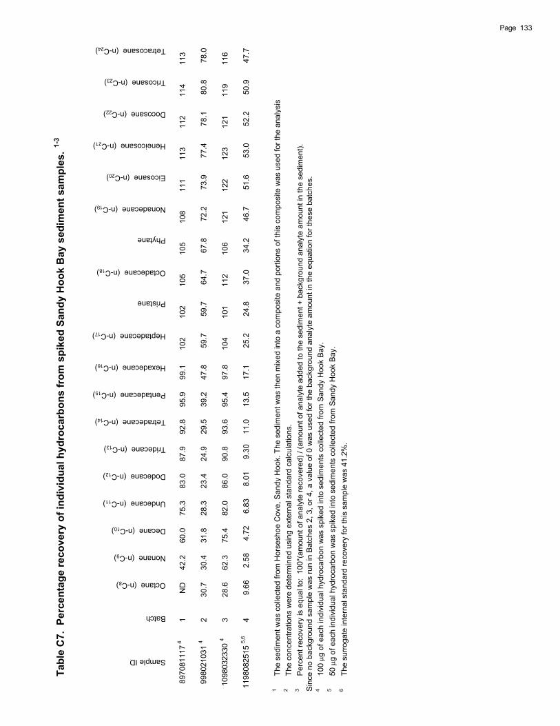
Tabl

e C

7. P

erce

ntag

e re

cove

ry o

f ind

ivid

ual h

ydro

carb

ons

from

spi

ked

Sand

y H

ook

Bay

sed

imen

t sam

ples

. 1-3

Sample ID

Batch

Octane (n-C8)

Nonane (n-C9)

Decane (n-C10)

Undecane (n-C11)

Dodecane (n-C12)

Tridecane (n-C13)

Tetradecane (n-C14)

Pentadecane (n-C15)

Hexadecane (n-C16)

Heptadecane (n-C17)

Pristane

Octadecane (n-C18)

Phytane

Nonadecane (n-C19)

Eicosane (n-C20)

Heneicosane (n-C21)

Docosane (n-C22)

Tricosane (n-C23)

Tetracosane (n-C24)

8970

8111

7 41

N

D

42

.2

60

.0

75

.3

83

.0

87

.9

92

.8

95

.9

99

.1

1

02

1

02

1

05

1

05

1

08

1

11

1

13

1

12

1

14

1

13

9980

2103

14

2

30.7

30.4

31.8

28.3

23.4

24.9

29.5

39.2

47.8

59.

7

59.

7

64.

7

67.

8

72.

2

73.

9

77.

4

78.

1

80.

8

78.

0

1098

0323

304

3

28.6

62.3

75.4

82.0

86.0

90.8

93.6

95.4

97.8

104

101

112

106

121

122

123

121

119

116

1198

0825

155,

64

9

.66

2

.58

4

.72

6

.83

8

.01

9

.30

1

1.0

1

3.5

1

7.1

2

5.2

2

4.8

3

7.0

3

4.2

4

6.7

5

1.6

5

3.0

5

2.2

5

0.9

4

7.7

1

The

sedi

men

t was

col

lect

ed fr

om H

orse

shoe

Cov

e, S

andy

Hoo

k. T

he s

edim

ent w

as th

en m

ixed

into

a c

ompo

site

and

por

tions

of t

his

com

posi

te w

as u

sed

for t

he a

naly

sis

2

The

conc

entra

tions

wer

e de

term

ined

usi

ng e

xter

nal s

tand

ard

calc

ulat

ions

. 3

P

erce

nt re

cove

ry is

equ

al to

: 10

0*(a

mou

nt o

f ana

lyte

reco

vere

d) /

(am

ount

of a

naly

te a

dded

to th

e se

dim

ent +

bac

kgro

und

anal

yte

amou

nt in

the

sedi

men

t).S

ince

no

back

grou

nd s

ampl

e w

as ru

n in

Bat

ches

2, 3

, or 4

, a v

alue

of 0

was

use

d fo

r the

bac

kgro

und

anal

yte

amou

nt in

the

equa

tion

for t

hese

bat

ches

.4

10

0 g

of e

ach

indi

vidu

al h

ydro

carb

on w

as s

pike

d in

to s

edim

ents

col

lect

ed fr

om S

andy

Hoo

k B

ay.

5

50

g of

eac

h in

divi

dual

hyd

roca

rbon

was

spi

ked

into

sed

imen

ts c

olle

cted

from

San

dy H

ook

Bay

.6

Th

e su

rrog

ate

inte

rnal

sta

ndar

d re

cove

ry fo

r thi

s sa

mpl

e w

as 4

1.2%

.

133Page

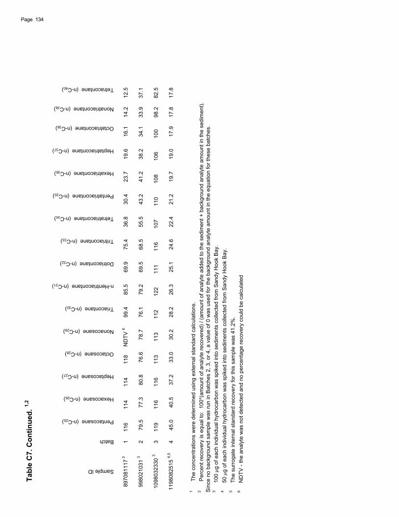
Tabl

e C

7. C

ontin

ued.

1,2

Sample ID

Batch

Pentacosane (n-C25)

Hexacosane (n-C26)

Heptacosane (n-C27)

Octacosane (n-C28)

Nonacosane (n-C29)

Triacontane (n-C30)

n-Hentriacontane (n-C31)

Dotriacontane (n-C32)

Tritriacontane (n-C33)

Tetratriacontane (n-C34)

Pentatriacontane (n-C35)

Hexatriacontane (n-C36)

Heptatriacontane (n-C37)

Octatriacontane (n-C38)

Nonatriacontane (n-C39)

Tetracontane (n-C40)

8970

8111

7 31

116

114

114

118

N

DTV

6

99.

4

85.

5

69.

9

75.

4

36.

8

30.

4

23.

7

19.

6

16.

1

14.

2

12.

5

9980

2103

13

2 7

9.5

7

7.3

8

0.8

7

6.6

7

8.7

7

6.1

7

9.2

6

9.5

6

8.5

5

5.5

4

3.2

4

1.2

3

8.2

3

4.1

3

3.9

3

7.1

1098

0323

303

3 1

19

1

16

1

16

1

13

1

13

1

12

1

22

1

11

1

16

1

07

1

10

1

08

1

06

1

00

9

8.2

8

2.5

1198

0825

154,

54

45.

0

40.

5

37.

2

33.

0

30.

2

28.

2

26.

3

25.

1

24.

6

22.

4

21.

2

19.

7

19.

0

17.

9

17.

8

17.

8

1

The

conc

entra

tions

wer

e de

term

ined

usi

ng e

xter

nal s

tand

ard

calc

ulat

ions

. 2

P

erce

nt re

cove

ry is

equ

al to

: 10

0*(a

mou

nt o

f ana

lyte

reco

vere

d) /

(am

ount

of a

naly

te a

dded

to th

e se

dim

ent +

bac

kgro

und

anal

yte

amou

nt in

the

sedi

men

t).S

ince

no

back

grou

nd s

ampl

e w

as ru

n in

Bat

ches

2, 3

, or 4

, a v

alue

of 0

was

use

d fo

r the

bac

kgro

und

anal

yte

amou

nt in

the

equa

tion

for t

hese

bat

ches

.3

100

g

of e

ach

indi

vidu

al h

ydro

carb

on w

as s

pike

d in

to s

edim

ents

col

lect

ed fr

om S

andy

Hoo

k B

ay.

4 5

0 g

of e

ach

indi

vidu

al h

ydro

carb

on w

as s

pike

d in

to s

edim

ents

col

lect

ed fr

om S

andy

Hoo

k B

ay.

5 T

he s

urro

gate

inte

rnal

sta

ndar

d re

cove

ry fo

r thi

s sa

mpl

e w

as 4

1.2%

.6

ND

TV -

the

anal

yte

was

not

det

ecte

d an

d no

per

cent

age

reco

very

cou

ld b

e ca

lcul

ated

.

Page 134

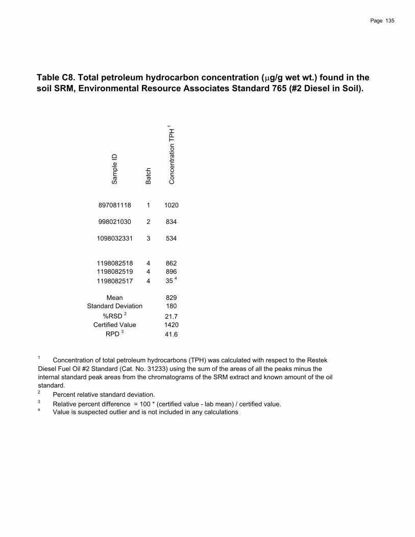
Table C8. Total petroleum hydrocarbon concentration ( g/g wet wt.) found in the soil SRM, Environmental Resource Associates Standard 765 (#2 Diesel in Soil).

Sam

ple

ID

Batc

h

Con

cent

ratio

n TP

H 1

897081118 1 1020

998021030 2 834

1098032331 3 534

1198082518 4 8621198082519 4 8961198082517 4 35 4

Mean 829Standard Deviation 180

%RSD 2 21.7Certified Value 1420

RPD 3 41.6

1 Concentration of total petroleum hydrocarbons (TPH) was calculated with respect to the RestekDiesel Fuel Oil #2 Standard (Cat. No. 31233) using the sum of the areas of all the peaks minus theinternal standard peak areas from the chromatograms of the SRM extract and known amount of the oilstandard.2 Percent relative standard deviation.3 Relative percent difference = 100 * (certified value - lab mean) / certified value.4 Value is suspected outlier and is not included in any calculations

135Page

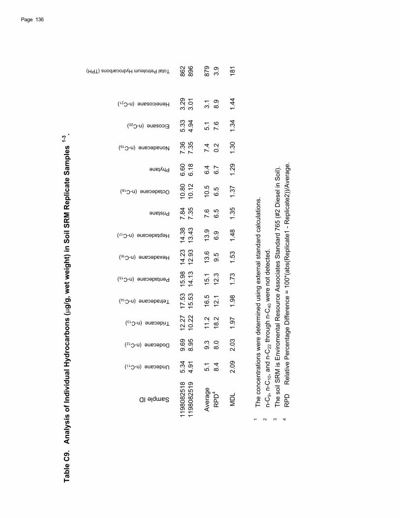
Page 136

Tabl

e C

9.

Ana

lysi

s of

Indi

vidu

al H

ydro

carb

ons

(g/

g, w

et w

eigh

t) in

Soi

l SR

M R

eplic

ate

Sam

ples

1-3 .

Sample ID

Undecane (n-C11)

Dodecane (n-C12)

Tridecane (n-C13)

Tetradecane (n-C14)

Pentadecane (n-C15)

Hexadecane (n-C16)

Heptadecane (n-C17)

Pristane

Octadecane (n-C18)

Phytane

Nonadecane (n-C19)

Eicosane (n-C20)

Heneicosane (n-C21)

Total Petroleum Hydrocarbons (TPH)

1198

0825

185.

349.

6912

.27

17.5

315

.98

14.2

314

.38

7.84

10.8

06.

607.

365.

333.

2986

211

9808

2519

4.91

8.95

10.2

215

.53

14.1

312

.93

13.4

37.

3510

.12

6.18

7.35

4.94

3.01

896

Ave

rage

5.1

9.3

11.2

16.5

15.1

13.6

13.9

7.6

10.5

6.4

7.4

5.1

3.1

879

RP

D4

8.4

8.0

18.2

12.1

12.3

9.5

6.9

6.5

6.5

6.7

0.2

7.6

8.9

3.9

MD

L2.

092.

031.

971.

981.

731.

531.

481.

351.

371.

291.

301.

341.

4418

1

1

The

conc

entra

tions

wer

e de

term

ined

usi

ng e

xter

nal s

tand

ard

calc

ulat

ions

. 2

n-

C9,

n-C

10, a

nd n

-C22

thro

ugh

n-C

40 w

ere

not d

etec

ted.

3

The

soil

SR

M is

Env

irom

enta

l Res

ourc

e A

ssoc

iate

s S

tand

ard

765

(#2

Die

sel i

n S

oil).

4

RP

D

Rel

ativ

e P

erce

ntag

e D

iffer

ence

= 1

00*(

abs(

Rep

licat

e1 -

Rep

licat

e2))

/Ave

rage

.

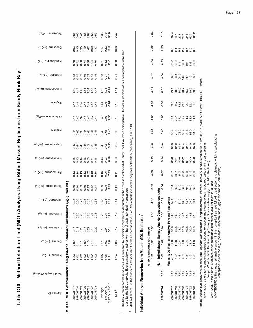
137Page

Tabl

e C

10.

Met

hod

Det

ectio

n Li

mit

(MD

L) A

naly

sis

Usi

ng R

ibbe

d-M

usse

l Rep

licat

es fr

om S

andy

Hoo

k B

ay.1

Sample ID

Total Sample Wt (in g)

Nonane (n-C9)

Decane (n-C10)

Undecane (n-C11)

Dodecane (n-C12)

Tridecane (n-C13)

Tetradecane (n-C14)

Pentadecane (n-C15)

Hexadecane (n-C16)

Heptadecane (n-C17)

Pristane

Octadecane (n-C18)

Phytane

Nonadecane (n-C19)

Eicosane (n-C20)

Heneicosane (n-C21)

Docosane (n-C22)

Tricosane (n-C23)

Mus

sel

MD

L D

eter

min

atio

n U

sing

Inte

rnal

Sta

ndar

d C

alcu

latio

ns (

g/g,

wet

wt.)

2970

3171

70.

230.

090.

150.

180.

230.

360.

430.

450.

470.

430.

440.

450.

490.

480.

700.

930.

5629

7031

718

0.02

0.11

0.19

0.25

0.30

0.40

0.44

0.43

0.44

0.40

0.40

0.41

0.47

0.45

0.72

0.95

0.83

2970

3171

90.

020.

110.

200.

230.

270.

330.

430.

440.

480.

380.

390.

390.

450.

520.

881.

351.

4129

7031

720

0.02

0.09

0.15

0.19

0.25

0.36

0.43

0.46

0.48

0.45

0.45

0.46

0.51

0.56

0.74

1.19

1.68

2970

3172

10.

020.

150.

270.

280.

330.

430.

520.

500.

520.

460.

460.

470.

540.

590.

861.

422.

0729

7031

722

0.02

0.11

0.19

0.24

0.30

0.42

0.49

0.51

0.51

0.47

0.47

0.46

0.53

0.61

1.04

0.99

2.58

2970

3172

30.

020.

110.

200.

260.

310.

410.

460.

460.

480.

410.

410.

410.

470.

450.

751.

370.

53

Ave

rage

0.05

0.11

0.19

0.23

0.28

0.39

0.46

0.46

0.48

0.43

0.43

0.44

0.50

0.53

0.81

1.17

1.38

Std

Dev

()

0.08

0.02

0.04

0.04

0.03

0.04

0.04

0.03

0.03

0.03

0.03

0.03

0.03

0.07

0.12

0.22

0.79

%R

SD

or %

CV

1

47

1

8.6

2

0.1

1

5.8

1

2.2

9.33

7.73

6.18

5.50

7.40

7.35

6.94

6.98

1

2.6

1

5.0

1

8.5

5

6.9

MD

L20.

240.

060.

120.

120.

110.

110.

110.

090.

080.

100.

100.

100.

110.

210.

380.

682.

47

1 T

he ti

ssue

mat

rix fo

r the

se s

ampl

es w

as p

repa

red

by c

ombi

ning

toge

ther

12

depu

rate

d rib

bed

mus

sels

col

lect

ed a

t San

dy H

ook

Bay

into

a h

omog

enat

e. I

ndiv

idua

l por

tions

of t

his

hom

ogen

ate

wer

e th

en

u

sed

for t

he M

DL

anal

ysis

. Eac

h sa

mpl

e w

as s

pike

d w

ith 4

g of

eac

h in

divi

dual

hyd

roca

rbon

.2

MD

L=t;

whe

re

is th

e st

anda

rd d

evia

tion

and

t is

the

Stu

dent

s t v

alue

. Fo

r 99%

con

fiden

ce le

vel,

6 de

gree

s of

free

dom

(one

-taile

d), t

= 3

.143

.

Indi

vidu

al A

naly

te R

ecov

erie

s fr

om M

usse

l MD

L R

eplic

ates

3

Ana

lyte

Am

ount

s (

g) A

dded

3.99

3.99

3.96

4.03

4.03

3.99

4.03

3.99

4.02

4.01

4.03

4.00

4.03

4.02

4.04

4.02

4.04

Non

-Spi

ked

Mus

sel S

ampl

e A

naly

te C

once

ntra

tions

(g/

g)29

7031

724

7.99

0.02

0.02

0.04

0.03

0.01

0.04

0.02

0.04

0.04

0.00

0.00

0.00

0.02

0.04

0.29

0.35

0.10

Mus

sel M

DL

Rep

licat

e A

naly

te P

erce

nt R

ecov

erie

s29

7031

717

7.97

4

3.7

1

7.6

2

8.9

3

3.3

4

4.4

6

7.4

8

1.7

8

3.6

8

5.6

8

5.4

8

7.0

8

9.8

9

3.1

8

9.0

8

8.0

1

08

9

2.4

2970

3171

87.

99

4.

51

20.

8

36.

5

46.

9

57.

8

73.

5

83.

7

79.

1

81.

0

78.

4

79.

1

82.

7

88.

0

83.

4

90.

8

111

137

29

7031

719

7.99

4.51

2

0.4

3

8.3

4

3.4

5

1.9

6

1.9

8

0.7

8

0.9

8

7.6

7

6.2

7

7.2

7

8.6

8

4.9

9

6.2

1

11

1

58

2

33

2970

3172

07.

99

4.

51

17.

8

27.

6

35.

1

48.

8

66.

3

81.

0

85.

2

88.

4

88.

4

89.

4

92.

0

96.

2

104

94.

1

139

277

29

7031

721

7.97

4.51

2

9.4

4

9.8

5

2.1

6

3.5

7

9.9

9

7.5

9

1.7

9

5.1

9

0.6

9

1.6

9

2.9

1

03

1

09

1

08

1

66

3

41

2970

3172

27.

99

4.

51

21.

3

36.

0

43.

9

58.

0

78.

0

93.

5

93.

3

94.

0

92.

5

92.

8

92.

4

99.

8

113

132

115

425

29

7031

723

7.98

4.51

2

1.3

3

6.8

4

7.9

5

9.1

7

5.3

8

7.9

8

4.8

8

7.3

8

1.3

8

1.5

8

1.3

8

9.2

8

3.7

9

4.9

1

60

8

7.2

3 T

he m

usse

l ana

lyte

reco

verie

s in

eac

h M

DL

repl

icat

e w

as c

alcu

late

d us

ing

the

form

ula:

P

erce

nt R

ecov

ery

is c

alcu

late

d as

100

* A

MTM

DL

/ (A

MN

TAD

D +

AM

NTB

KG

RD

) w

here

AM

NTM

DL

is th

e an

alyt

e am

ount

mea

sure

d fo

llow

ng e

xtra

ctio

n an

d cl

eanu

p of

eac

h M

DL

repl

icat

e, w

hich

is c

alcu

late

d as

(S

ampl

e W

t of t

he M

DL

Rep

licat

e in

g) *

(Ana

lyte

Con

cent

ratio

n in

g/g

in th

e M

DL

Rep

licat

e);

AM

NTA

DD

is th

e am

ount

of a

naly

te a

dded

to th

e un

spik

ed m

usse

l MD

L re

plic

ate

in g

; an

d

A

MN

TBK

GR

D is

the

mea

sure

d an

alyt

e am

ount

in th

e no

n-sp

iked

sam

ple

follo

win

g ex

tract

ion

and

clea

nup,

whi

ch is

cal

cula

ted

as

(

Non

-spi

ked

Sam

ple

Wt i

n g)

* (A

naly

te C

once

ntra

tion

in

g/g

in th

e N

on-s

pike

d S

ampl

e).

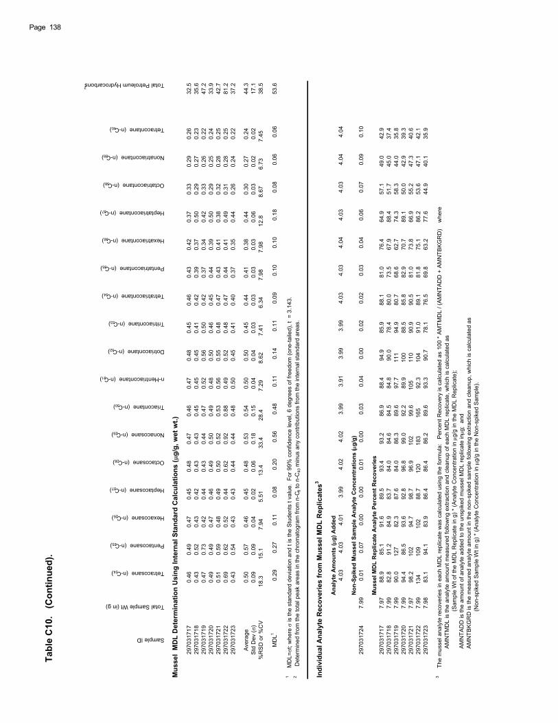
Page 138

Tabl

e C

10.

(Con

tinue

d).

Sample ID

Total Sample Wt (in g)

Tetracosane (n-C24)

Pentacosane (n-C25)

Hexacosane (n-C26)

Heptacosane (n-C27)

Octacosane (n-C28)

Nonacosane (n-C29)

Triacontane (n-C30)

n-Hentriacontane (n-C31)

Dotriacontane (n-C32)

Tritriacontane (n-C33)

Tetratriacontane (n-C34)

Pentatriacontane (n-C35)

Hexatriacontane (n-C36)

Heptatriacontane (n-C37)

Octatriacontane (n-C38)

Nonatriacontane (n-C39)

Tetracontane (n-C40)

Total Petroleum Hydrocarbons2

Mus

sel

MD

L D

eter

min

atio

n U

sing

Inte

rnal

Sta

ndar

d C

alcu

latio

ns (

g/g,

wet

wt.)

2970

3171

70.

460.

490.

470.

450.

480.

470.

460.

470.

480.

450.

460.

430.

420.

370.

330.

290.

26

32

.529

7031

718

0.43

0.52

0.43

0.42

0.43

0.43

0.45

0.45

0.45

0.41

0.42

0.39

0.37

0.50

0.29

0.27

0.23

35.6

2970

3171

90.

470.

730.

420.

440.

430.

440.

470.

520.

560.

500.

420.

370.

340.

420.

330.

260.

22

47

.229

7031

720

0.49

0.49

0.47

0.46

0.49

0.50

0.49

0.48

0.50

0.46

0.45

0.44

0.39

0.50

0.29

0.25

0.24

33.9

2970

3172

10.

510.

590.

480.

490.

500.

520.

530.

560.

550.

480.

470.

430.

410.

380.

320.

280.

25

42

.729

7031

722

0.69

0.62

0.52

0.44

0.62

0.92

0.88

0.49

0.52

0.48

0.47

0.44

0.41

0.49

0.31

0.28

0.25

81.2

2970

3172

30.

430.

540.

430.

430.

440.

440.

480.

500.

450.

410.

400.

370.

350.

440.

260.

240.

22

37

.2

Ave

rage

0.50

0.57

0.46

0.45

0.48

0.53

0.54

0.50

0.50

0.45

0.44

0.41

0.38

0.44

0.30

0.27

0.24

44.3

Std

Dev

()

0.09

0.09

0.04

0.02

0.06

0.18

0.15

0.04

0.04

0.03

0.03

0.03

0.03

0.06

0.03

0.02

0.02

17.1

%R

SD

or %

CV

1

8.3

1

5.1

7.94

5.51

1

3.4

3

3.4

2

8.4

7.29

8.62

7.41

6.34

7.98

7.98

1

2.8

8.67

6.73

7.45

38.5

MD

L10.

290.

270.

110.

080.

200.

560.

480.

110.

140.

110.

090.

100.

100.

180.

080.

060.

06

53

.6

1 M

DL=

t; w

here

is

the

stan

dard

dev

iatio

n an

d t i

s th

e S

tude

nts

t val

ue.

For 9

9% c

onfid

ence

leve

l, 6

degr

ees

of fr

eedo

m (o

ne-ta

iled)

, t =

3.1

43.

2

Det

erm

ined

from

the

tota

l pea

k ar

eas

in th

e ch

rom

atog

ram

from

n-C

8 to

n-C

40 m

inus

any

con

tribu

tions

from

the

inte

rnal

sta

ndar

d ar

eas.

Indi

vidu

al A

naly

te R

ecov

erie

s fr

om M

usse

l MD

L R

eplic

ates

3

Ana

lyte

Am

ount

s (

g) A

dded

4.03

4.03

4.01

3.99

4.02

4.02

3.99

3.91

3.99

3.99

4.03

4.03

4.04

4.03

4.03

4.04

4.04

Non

-Spi

ked

Mus

sel S

ampl

e A

naly

te C

once

ntra

tions

(g/

g)29

7031

724

7.99

0.01

0.07

0.00

0.00

0.01

0.00

0.03

0.04

0.00

0.02

0.02

0.03

0.04

0.06

0.07

0.09

0.10

Mus

sel M

DL

Rep

licat

e A

naly

te P

erce

nt R

ecov

erie

s29

7031

717

7.97

8

8.9

8

5.1

9

1.6

8

9.5

9

3.4

9

3.2

8

6.9

8

8.4

9

4.9

8

5.9

8

8.1

8

1.0

7

6.4

6

4.9

5

7.1

4

9.0

4

2.9

2970

3171

87.

99

82.

8

91.

2

84.

9

83.

7

84.

0

84.

6

84.

5

84.

8

90.

0

78.

4

80.

0

73.

5

67.

9

88.

4

51.

7

45.

0

37.

4 29

7031

719

7.99

9

0.0

1

27

8

2.3

8

7.6

8

4.0

8

6.3

8

9.6

9

7.7

1

11

9

4.9

8

0.7

6

8.6

6

2.7

7

4.3

5

8.3

4

4.0

3

5.8

2970

3172

07.

99

94.

4

86.

5

93.

6

92.

8

96.

8

99.

0

92.

2

89.

9

100

88.

5

85.

8

82.

9

70.

7

89.

1

50.

0

42.

9

39.

3 29

7031

721

7.97

9

8.2

1

02

9

4.7

9

8.7

9

6.9

1

02

9

9.6

1

05

1

10

9

0.9

9

0.5

8

1.0

7

3.8

6

6.9

5

5.2

4

7.3

4

0.6

2970

3172

27.

99

134

109

102

88.

7

120

183

165

92.

3

104

91.

0

89.

1

81.

8

75.

1

86.

2

53.

6

47.

1

42.

1 29

7031

723

7.98

8

3.1

9

4.1

8

3.9

8

6.4

8

6.4

8

6.2

8

9.6

9

3.3

9

0.7

7

8.1

7

6.5

6

9.8

6

3.2

7

7.6

4

4.9

4

0.1

3

5.9

3 T

he m

usse

l ana

lyte

reco

verie

s in

eac

h M

DL

repl

icat

e w

as c

alcu

late

d us

ing

the

form

ula:

P

erce

nt R

ecov

ery

is c

alcu

late

d as

100

* A

MTM

DL

/ (A

MN

TAD

D +

AM

NTB

KG

RD

) w

here

AM

NTM

DL

is th

e an

alyt

e am

ount

mea

sure

d fo

llow

ng e

xtra

ctio

n an

d cl

eanu

p of

eac

h M

DL

repl

icat

e, w

hich

is c

alcu

late

d as

(S

ampl

e W

t of t

he M

DL

Rep

licat

e in

g) *

(Ana

lyte

Con

cent

ratio

n in

g/

g in

the

MD

L R

eplic

ate)

;

A

MN

TAD

D is

the

amou

nt o

f ana

lyte

add

ed to

the

unsp

iked

mus

sel M

DL

repl

icat

e in

g;

and

AM

NTB

KG

RD

is th

e m

easu

red

anal

yte

amou

nt in

the

non-

spik

ed s

ampl

e fo

llow

ing

extra

ctio

n an

d cl

eanu

p, w

hich

is c

alcu

late

d as

(N

on-s

pike

d S

ampl

e W

t in

g) *

(Ana

lyte

Con

cent

ratio

n in

g/

g in

the

Non

-spi

ked

Sam

ple)

.

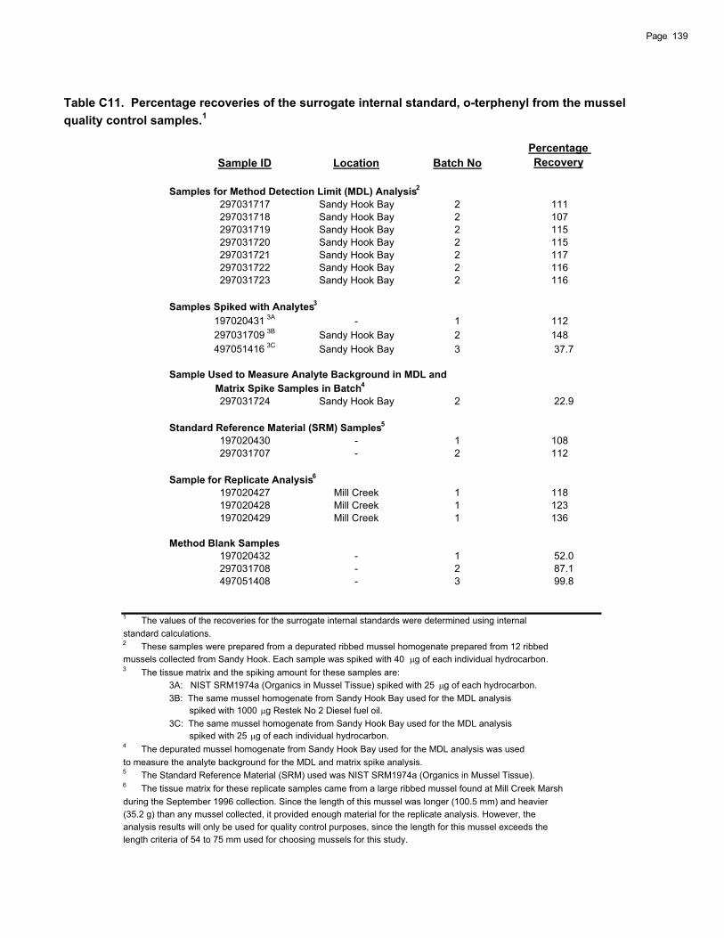
Table C11. Percentage recoveries of the surrogate internal standard, o-terphenyl from the mussel quality control samples.1

Sample ID Location Batch NoPercentageRecovery

Samples for Method Detection Limit (MDL) Analysis2

297031717 Sandy Hook Bay 2 111 297031718 Sandy Hook Bay 2 107 297031719 Sandy Hook Bay 2 115 297031720 Sandy Hook Bay 2 115 297031721 Sandy Hook Bay 2 117 297031722 Sandy Hook Bay 2 116 297031723 Sandy Hook Bay 2 116

Samples Spiked with Analytes3

197020431 3A - 1 112 297031709 3B Sandy Hook Bay 2 148 497051416 3C Sandy Hook Bay 3 37.7

Sample Used to Measure Analyte Background in MDL andMatrix Spike Samples in Batch4

297031724 Sandy Hook Bay 2 22.9

Standard Reference Material (SRM) Samples5

197020430 - 1 108 297031707 - 2 112

Sample for Replicate Analysis6

197020427 Mill Creek 1 118 197020428 Mill Creek 1 123 197020429 Mill Creek 1 136

Method Blank Samples 197020432 - 1 52.0 297031708 - 2 87.1 497051408 - 3 99.8

1 The values of the recoveries for the surrogate internal standards were determined using internalstandard calculations.2 These samples were prepared from a depurated ribbed mussel homogenate prepared from 12 ribbed mussels collected from Sandy Hook. Each sample was spiked with 40 g of each individual hydrocarbon.3 The tissue matrix and the spiking amount for these samples are:

3A: NIST SRM1974a (Organics in Mussel Tissue) spiked with 25 g of each hydrocarbon.3B: The same mussel homogenate from Sandy Hook Bay used for the MDL analysis spiked with 1000 g Restek No 2 Diesel fuel oil.3C: The same mussel homogenate from Sandy Hook Bay used for the MDL analysis spiked with 25 g of each individual hydrocarbon.

4 The depurated mussel homogenate from Sandy Hook Bay used for the MDL analysis was used to measure the analyte background for the MDL and matrix spike analysis.5 The Standard Reference Material (SRM) used was NIST SRM1974a (Organics in Mussel Tissue).6 The tissue matrix for these replicate samples came from a large ribbed mussel found at Mill Creek Marsh during the September 1996 collection. Since the length of this mussel was longer (100.5 mm) and heavier(35.2 g) than any mussel collected, it provided enough material for the replicate analysis. However, theanalysis results will only be used for quality control purposes, since the length for this mussel exceeds the length criteria of 54 to 75 mm used for choosing mussels for this study.

139Page

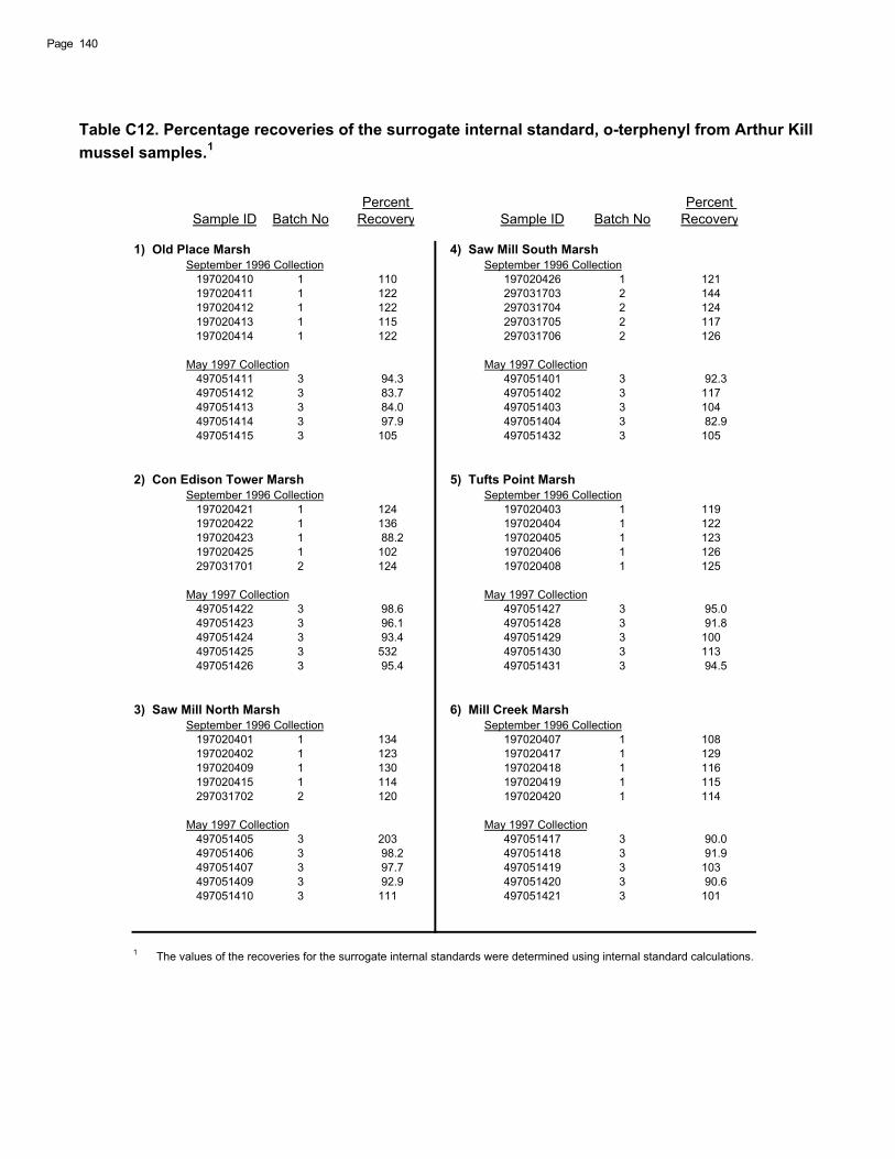
Table C12. Percentage recoveries of the surrogate internal standard, o-terphenyl from Arthur Kill mussel samples.1

Sample ID Batch NoPercent

Recovery Sample ID Batch NoPercent

Recovery

1) Old Place Marsh 4) Saw Mill South MarshSeptember 1996 Collection September 1996 Collection

197020410 1 110 197020426 1 121 197020411 1 122 297031703 2 144 197020412 1 122 297031704 2 124 197020413 1 115 297031705 2 117 197020414 1 122 297031706 2 126

May 1997 Collection May 1997 Collection497051411 3 94.3 497051401 3 92.3 497051412 3 83.7 497051402 3 117 497051413 3 84.0 497051403 3 104 497051414 3 97.9 497051404 3 82.9 497051415 3 105 497051432 3 105

2) Con Edison Tower Marsh 5) Tufts Point MarshSeptember 1996 Collection September 1996 Collection

197020421 1 124 197020403 1 119 197020422 1 136 197020404 1 122 197020423 1 88.2 197020405 1 123 197020425 1 102 197020406 1 126 297031701 2 124 197020408 1 125

May 1997 Collection May 1997 Collection497051422 3 98.6 497051427 3 95.0 497051423 3 96.1 497051428 3 91.8 497051424 3 93.4 497051429 3 100 497051425 3 532 497051430 3 113 497051426 3 95.4 497051431 3 94.5

3) Saw Mill North Marsh 6) Mill Creek MarshSeptember 1996 Collection September 1996 Collection

197020401 1 134 197020407 1 108 197020402 1 123 197020417 1 129 197020409 1 130 197020418 1 116 197020415 1 114 197020419 1 115 297031702 2 120 197020420 1 114

May 1997 Collection May 1997 Collection497051405 3 203 497051417 3 90.0 497051406 3 98.2 497051418 3 91.9 497051407 3 97.7 497051419 3 103 497051409 3 92.9 497051420 3 90.6 497051410 3 111 497051421 3 101

1 The values of the recoveries for the surrogate internal standards were determined using internal standard calculations.

Page 140

Table C13. Percentage recoveries of the surrogate internal standard, o-terphenyl from mussels from Sandy Hook Bay.1,2

Sample ID Batch NoPercent

Recovery

297031710 2 135 297031711 2 142 297031712 2 130 297031713 2 136 297031714 2 128 297031715 2 131 297031716 2 134

1 The values of the recoveries for the surrogate internal standards were determined using internal standard calculations.2 Each of these mussel samples is an individual, non-depurated, ribbed mussel takenfrom Sandy Hook Bay on February 20, 1997.

141Page

Tabl

e C

14.

Perc

ent R

ecov

ery

of In

divi

dual

Hyd

roca

rbon

s an

d D

iese

l Fue

l fro

m S

pike

d R

ibbe

d M

usse

l Sam

ples

.Sample ID

Batch No

Tissue Matrix

Nonane (n-C9)

Decane (n-C10)

Undecane (n-C11)

Dodecane (n-C12)

Tridecane (n-C13)

Tetradecane (n-C14)

Pentadecane (n-C15)

Hexadecane (n-C16)

Heptadecane (n-C17)

Pristane

Octadecane (n-C18)

Phytane

Nonadecane (n-C19)

Eicosane (n-C20)

Heneicosane (n-C21)

Docosane (n-C22)

Tricosane (n-C23)

Tetracosane (n-C24)

Pentacosane (n-C25)

1970

2043

111

NIS

T S

RM

1974

a10

.341

.354

.968

.778

.083

.686

.487

.484

.986

.888

.087

.093

.689

.780

.188

.290

.891

.492

.4

2970

3170

92-

42

Dep

urat

ed M

usse

l H

omog

enat

e

185

23.

6

52.

1

57.

9

62.

0

81.

2

82.

0

94.

1

87.

9

81.

2

81.

9

74.

2

93.

4

100

569

650

1740

318

0.0

0

4970

5141

65

3D

epur

ated

Mus

sel

Hom

ogen

ate

7

.70

4

.16

8

.00

1

3.9

2

6.9

4

7.2

6

2.5

7

4.9

7

9.9

7

9.2

8

3.6

8

2.1

8

2.1

8

6.9

13

1

10

0

9

0.9

8

8.2

8

8.4

1

25g

of e

ach

indi

vidu

al h

ydro

carb

on w

as s

pike

d in

to a

tis

sue

mat

rix m

ade

from

NIS

T S

RM

1974

a (O

rgan

ics

in M

usse

l).2

10

00g

of R

este

k D

iese

l Fue

l Oil

#2 S

tand

ard

(Cat

. No

3123

3) w

as s

pike

d in

to a

mus

sel t

issu

e ho

mog

enat

e pr

epar

ed fr

om ri

bbed

mus

sels

col

lect

ed fr

om S

andy

Hoo

k B

ay.

3

The

fuel

oil

will

ele

vate

the

leve

ls o

f the

indi

vidu

al h

ydro

carb

ons

n-C

8 th

roug

h n-

C26

, pris

tane

, and

phy

tane

onl

y. T

he re

cove

ries

of o

nly

thes

e hy

droc

arbo

ns a

re s

igni

fican

tly im

porta

nt.

4Th

e co

ncen

tratio

ns o

f the

indi

vidu

al h

ydro

carb

ons

wer

e no

t det

erm

ined

. Th

e re

cove

ries

of in

divi

dual

hyd

roca

rbon

s w

ere

calc

ulat

ed b

y co

mpa

ring

the

peak

are

as fo

r the

hyd

roca

rbon

s in

the

spik

ed e

xtra

ct to

thos

e in

the

Res

tek

oil s

tand

ard.

5

25g

of e

ach

indi

vidu

al h

ydro

carb

on w

as s

pike

d in

to a

mus

sel t

issu

e ho

mog

enat

e pr

epar

ed fr

om ri

bbed

mus

sels

col

lect

ed fr

om S

andy

Hoo

k B

ay.

Page 142

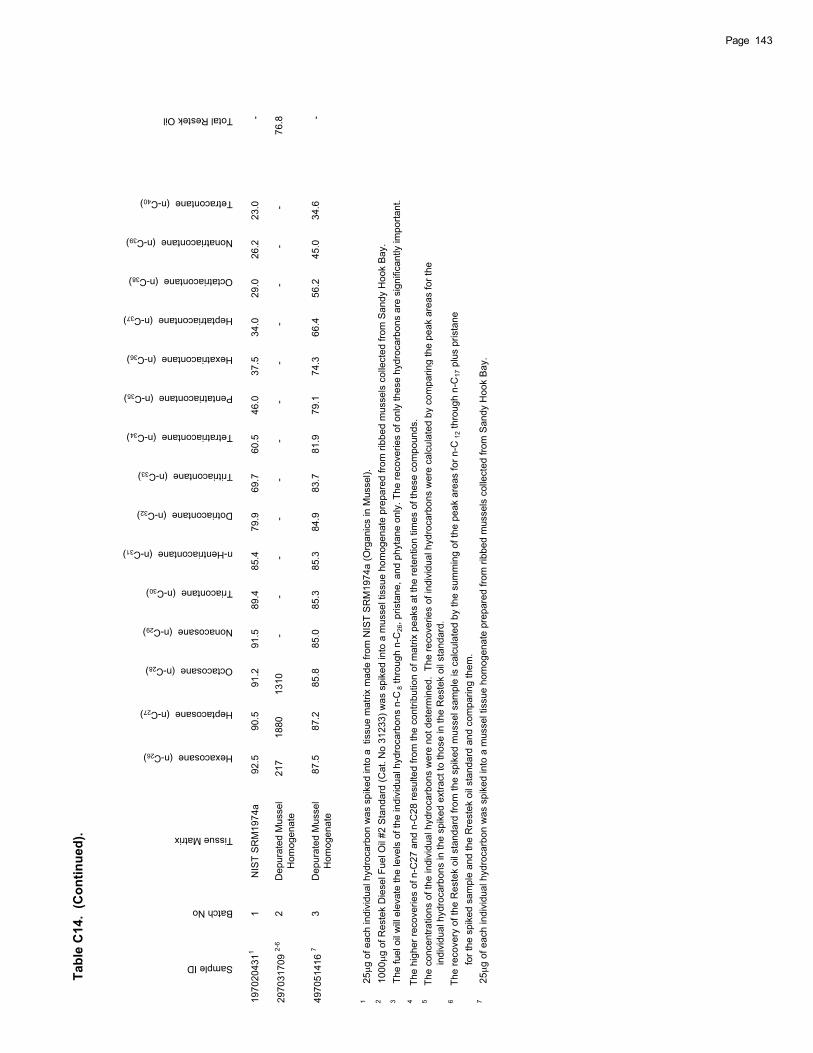
Tabl

e C

14.

(Con

tinue

d).

Sample ID

Batch No

Tissue Matrix

Hexacosane (n-C26)

Heptacosane (n-C27)

Octacosane (n-C28)

Nonacosane (n-C29)

Triacontane (n-C30)

n-Hentriacontane (n-C31)

Dotriacontane (n-C32)

Tritriacontane (n-C33)

Tetratriacontane (n-C34)

Pentatriacontane (n-C35)

Hexatriacontane (n-C36)

Heptatriacontane (n-C37)

Octatriacontane (n-C38)

Nonatriacontane (n-C39)

Tetracontane (n-C40)

Total Restek Oil

1970

2043

111

NIS

T S

RM

1974

a92

.590

.591

.291

.589

.485

.479

.969

.760

.546

.037

.534

.029

.026

.223

.0-

2970

3170

92-

62

Dep

urat

ed M

usse

l H

omog

enat

e

217

1880

1310

-

-

-

-

-

-

-

-

-

-

-

-

76

.8

4970

5141

67

3D

epur

ated

Mus

sel

Hom

ogen

ate

87.5

87.2

85.8

85.0

85.3

85.3

84.9

83.7

81.9

79.1

74.3

66.4

56.2

45.0

34.6

-

1

25g

of e

ach

indi

vidu

al h

ydro

carb

on w

as s

pike

d in

to a

tis

sue

mat

rix m

ade

from

NIS

T S

RM

1974

a (O

rgan

ics

in M

usse

l).2

10

00g

of R

este

k D

iese

l Fue

l Oil

#2 S

tand

ard

(Cat

. No

3123

3) w

as s

pike

d in

to a

mus

sel t

issu

e ho

mog

enat

e pr

epar

ed fr

om ri

bbed

mus

sels

col

lect

ed fr

om S

andy

Hoo

k B

ay.

3

The

fuel

oil

will

ele

vate

the

leve

ls o

f the

indi

vidu

al h

ydro

carb

ons

n-C

8 thr

ough

n-C

26, p

rista

ne, a

nd p

hyta

ne o

nly.

The

reco

verie

s of

onl

y th

ese

hydr

ocar

bons

are

sig

nific

antly

impo

rtant

.4

The

high

er re

cove

ries

of n

-C27

and

n-C

28 re

sulte

d fro

m th

e co

ntrib

utio

n of

mat

rix p

eaks

at t

he re

tent

ion

times

of t

hese

com

poun

ds.

5Th

e co

ncen

tratio

ns o

f the

indi

vidu

al h

ydro

carb

ons

wer

e no

t det

erm

ined

. Th

e re

cove

ries

of in

divi

dual

hyd

roca

rbon

s w

ere

calc

ulat

ed b

y co

mpa

ring

the

peak

are

as fo

r the

ind

ivid

ual h

ydro

carb

ons

in th

e sp

iked

ext

ract

to th

ose

in th

e R

este

k oi

l sta

ndar

d.6

The

reco

very

of t

he R

este

k oi

l sta

ndar

d fro

m th

e sp

iked

mus

sel s

ampl

e is

cal

cula

ted

by th

e su

mm

ing

of th

e pe

ak a

reas

for n

-C12

thro

ugh

n-C

17 p

lus

pris

tane

for

the

spik

ed s

ampl

e an

d th

e R

rest

ek o

il st

anda

rd a

nd c

ompa

ring

them

.7

25

g of

eac

h in

divi

dual

hyd

roca

rbon

was

spi

ked

into

a m

usse

l tis

sue

hom

ogen

ate

prep

ared

from

ribb

ed m

usse

ls c

olle

cted

from

San

dy H

ook

Bay

.

143Page

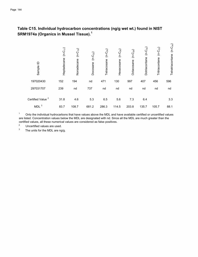
Table C15. Individual hydrocarbon concentrations (ng/g wet wt.) found in NIST SRM1974a (Organics in Mussel Tissue).1

Sam

ple

ID

Hep

tade

cane

(n-

C17

)

Non

adec

ane

(n-C

19)

Doc

osan

e (n

-C22

)

Tetra

cosa

ne (

n-C

24)

Hex

acos

ane

(n-C

26)

Oct

acos

ane

(n-C

28)

Dot

riaco

ntan

e (n

-C32

)

Tritr

iaco

ntan

e (n

-C33

)

Tetra

triac

onta

ne (

n-C

34)

197020430 152 194 nd 471 130 997 407 456 596

297031707 239 nd 737 nd nd nd nd nd nd

Certified Value 2 31.8 4.6 5.3 6.5 5.6 7.3 6.4 3.3

MDL 3 83.7 108.7 681.2 286.3 114.5 203.8 135.7 105.7 88.1

1 Only the individual hydrocarbons that have values above the MDL and have available certified or uncertified valuesare listed. Concentration values below the MDL are designated with nd. Since all the MDL are much greater than thecertified values, all these numerical values are considered as false positives.2 Uncertified values are used.3 The units for the MDL are ng/g.

Page 144

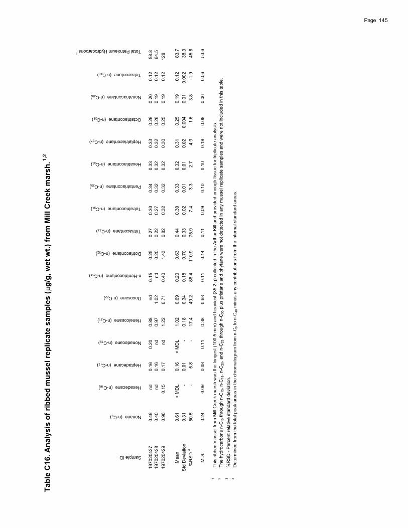
Tabl

e C

16. A

naly

sis

of ri

bbed

mus

sel r

eplic

ate

sam

ples

(g/

g, w

et w

t.) fr

om M

ill C

reek

mar

sh.1,

2

Sample ID

Nonane (n-C9)

Hexadecane (n-C16)

Heptadecane (n-C17)

Nonadecane (n-C19)

Heneicosane (n-C21)

Docosane (n-C22)

n-Hentriacontane (n-C31)

Dotriacontane (n-C32)

Tritriacontane (n-C33)

Tetratriacontane (n-C34)

Pentatriacontane (n-C35)

Hexatriacontane (n-C36)

Heptatriacontane (n-C37)

Octatriacontane (n-C38)

Nonatriacontane (n-C39)

Tetracontane (n-C40)

Total Petroleum Hydrocarbons 4

1970

2042

70.

46nd

0.16

0.20

0.88

nd0.

150.

250.

270.

300.

340.

330.

330.

260.

200.

12

58.

8 19

7020

428

0.40

nd0.

16nd

0.97

1.02

nd0.

200.

220.

270.

320.

320.

320.

260.

190.

12

64.

5 19

7020

429

0.96

0.15

0.17

nd1.

220.

710.

401.

430.

820.

320.

320.

320.

300.

250.

190.

12

128

Mea

n0.

61<

MD

L0.

16<

MD

L1.

020.

690.

200.

630.

440.

300.

330.

320.

310.

250.

190.

12

83

.7S

td D

evia

tion

0.31

-0.

01-

0.18

0.34

0.18

0.70

0.33

0.02

0.01

0.01

0.02

0.00

40.

010.

002

38.3

%R

SD

350

.5-

5.8

-17

.449

.288

.411

0.9

75.9

7.4

3.3

2.7

4.9

1.6

3.8

1.9

45.8

MD

L0.

240.

090.

080.

110.

380.

680.

110.

140.

110.

090.

100.

100.

180.

080.

060.

0653

.6

1

Thi

s rib

bed

mus

sel f

rom

Mill

Cre

ek m

arsh

was

the

long

est (

100.

5 m

m) a

nd h

eavi

est (

35.2

g) c

olle

cted

in th

e A

rthur

Kill

and

prov

ided

eno

ugh

tissu

e fo

r trip

licat

e an

alys

is.

2

The

hyd

roca

rbon

s n-

C 10 t

hrou

gh n

-C15

, n-C

18, n

-C20

, and

n-C

23 th

roug

h n-

C30

plu

s pr

ista

ne a

nd p

hyta

ne w

ere

not d

etec

ted

in a

ny m

usse

l rep

licat

e sa

mpl

es a

nd w

ere

not i

nclu

ded

in th

is ta

ble.

3

%R

SD

- P

erce

nt re

lativ

e st

anda

rd d

evia

tion.

4

Det

erm

ined

from

the

tota

l pea

k ar

eas

in th

e ch

rom

atog

ram

from

n-C

8 to

n-C

40 m

inus

any

con

tribu

tions

from

the

inte

rnal

sta

ndar

d ar

eas.

145Page

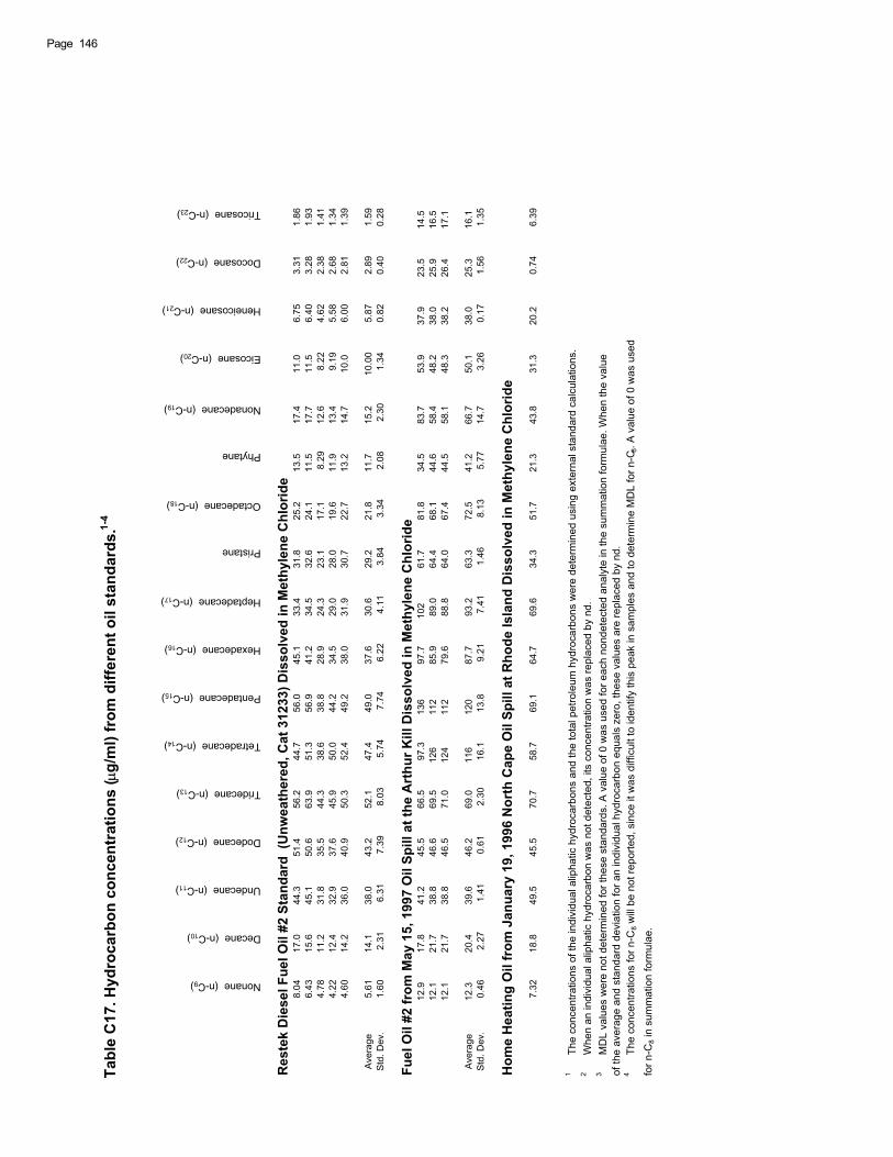
Tabl

e C

17. H

ydro

carb

on c

once

ntra

tions

(g/

ml)

from

diff

eren

t oil

stan

dard

s.1-

4

Nonane (n-C9)

Decane (n-C10)

Undecane (n-C11)

Dodecane (n-C12)

Tridecane (n-C13)

Tetradecane (n-C14)

Pentadecane (n-C15)

Hexadecane (n-C16)

Heptadecane (n-C17)

Pristane

Octadecane (n-C18)

Phytane

Nonadecane (n-C19)

Eicosane (n-C20)

Heneicosane (n-C21)

Docosane (n-C22)

Tricosane (n-C23)

Res

tek

Die

sel F

uel O

il #2

Sta

ndar

d (U

nwea

ther

ed, C

at 3

1233

) Dis

solv

ed in

Met

hyle

ne C

hlor

ide

8.04

1

7.0

4

4.3

5

1.4

5

6.2

4

4.7

5

6.0

4

5.1

3

3.4

3

1.8

2

5.2

1

3.5

1

7.4

1

1.0

6.75

3.31

1.86

6.43

1

5.6

4

5.1

5

0.6

6

3.9

5

1.3

5

6.9

4

1.2

3

4.5

3

2.6

2

4.1

1

1.5

1

7.7

1

1.5

6.40

3.28

1.93

4.78

1

1.2

3

1.8

3

5.5

4

4.3

3

8.6

3

8.8

2

8.9

2

4.3

2

3.1

1

7.1

8.29

1

2.6

8.22

4.62

2.38

1.41

4.22

1

2.4

3

2.9

3

7.6

4

5.9

5

0.0

4

4.2

3

4.5

2

9.0

2

8.0

1

9.6

1

1.9

1

3.4

9.19

5.58

2.68

1.34

4.60

1

4.2

3

6.0

4

0.9

5

0.3

5

2.4

4

9.2

3

8.0

3

1.9

3

0.7

2

2.7

1

3.2

1

4.7

1

0.0

6.00

2.81

1.39

Ave

rage

5.61

1

4.1

3

8.0

4

3.2

5

2.1

4

7.4

4

9.0

3

7.6

3

0.6

2

9.2

2

1.8

1

1.7

1

5.2

1

0.00

5.87

2.89

1.59

Std

. Dev

.

1.

60

2.

31

6.

31

7.

39

8.

03

5.

74

7.

74

6.

22

4.

11

3.

84

3.

34

2.

08

2.

30

1.

34

0.

82

0.

40

0.

28

Fuel

Oil

#2 fr

om M

ay 1

5, 1

997

Oil

Spill

at t

he A

rthu

r Kill

Dis

solv

ed in

Met

hyle

ne C

hlor

ide

1

2.9

1

7.8

4

1.2

4

5.5

6

6.5

9

7.3

1

36

9

7.7

1

02

6

1.7

8

1.8

3

4.5

8

3.7

5

3.9

3

7.9

2

3.5

1

4.5

1

2.1

2

1.7

3

8.8

4

6.6

6

9.5

1

26

1

12

8

5.9

8

9.0

6

4.4

6

8.1

4

4.6

5

8.4

4

8.2

3

8.0

2

5.9

1

6.5

1

2.1

2

1.7

3

8.8

4

6.5

7

1.0

1

24

1

12

7

9.6

8

8.8

6

4.0

6

7.4

4

4.5

5

8.1

4

8.3

3

8.2

2

6.4

1

7.1

Ave

rage

1

2.3

2

0.4

3

9.6

4

6.2

6

9.0

1

16

1

20

8

7.7

9

3.2

6

3.3

7

2.5

4

1.2

6

6.7

5

0.1

3

8.0

2

5.3

1

6.1

Std

. Dev

.

0.

46

2.

27

1.

41

0.

61

2.

30

16.

1

13.

8

9.

21

7.

41

1.

46

8.

13

5.

77

14.

7

3.

26

0.

17

1.

56

1.

35

Hom

e H

eatin

g O

il fr

om J

anua

ry 1

9, 1

996

Nor

th C

ape

Oil

Spill

at R

hode

Isla

nd D

isso

lved

in M

ethy

lene

Chl

orid

e

7.32

1

8.8

4

9.5

4

5.5

7

0.7

5

8.7

6

9.1

6

4.7

6

9.6

3

4.3

5

1.7

2

1.3

4

3.8

3

1.3

2

0.2

0.74

6.39

1

The

conc

entra

tions

of t

he in

divi

dual

alip

hatic

hyd

roca

rbon

s an

d th

e to

tal p

etro

leum

hyd

roca

rbon

s w

ere

dete

rmin

ed u

sing

ext

erna

l sta

ndar

d ca

lcul

atio

ns.

2

Whe

n an

indi

vidu

al a

lipha

tic h

ydro

carb

on w

as n

ot d

etec

ted,

its

conc

entra

tion

was

repl

aced

by

nd.

3

MD

L va

lues

wer

e no

t det

erm

ined

for t

hese

sta

ndar

ds. A

val

ue o

f 0 w

as u

sed

for e

ach

nond

etec

ted

anal

yte

in th

e su

mm

atio

n fo

rmul

ae. W

hen

the

valu

e of

the

aver

age

and

stan

dard

dev

iatio

n fo

r an

indi

vidu

al h

ydro

carb

on e

qual

s ze

ro, t

hese

val

ues

are

repl

aced

by

nd.

4

The

conc

entra

tions

for n

-C8 w

ill b

e no

t rep

orte

d, s

ince

it w

as d

iffic

ult t

o id

entif

y th

is p

eak

in s

ampl

es a

nd to

det

erm

ine

MD

L fo

r n-C

8. A

val

ue o

f 0 w

as u

sed

for n

-C8 i

n su

mm

atio

n fo

rmul

ae.

Page 146

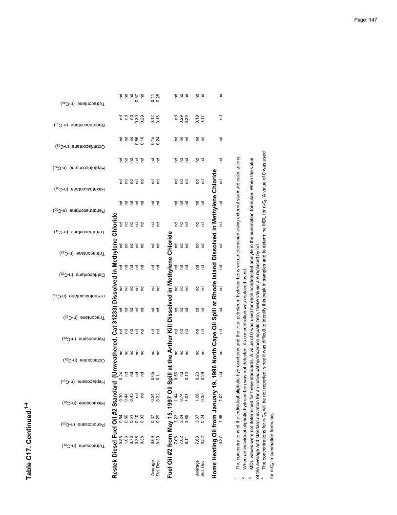
Tabl

e C

17. C

ontin

ued.

1-4

Tetracosane (n-C24)

Pentacosane (n-C25)

Hexacosane (n-C26)

Heptacosane (n-C27)

Octacosane (n-C28)

Nonacosane (n-C29)

Triacontane (n-C30)

n-Hentriacontane (n-C31)

Dotriacontane (n-C32)

Tritriacontane (n-C33)

Tetratriacontane (n-C34)

Pentatriacontane (n-C35)

Hexatriacontane (n-C36)

Heptatriacontane (n-C37)

Octatriacontane (n-C38)

Nonatriacontane (n-C39)

Tetracontane (n-C40)

Res

tek

Die

sel F

uel O

il #2

Sta

ndar

d (U

nwea

ther

ed, C

at 3

1233

) Dis

solv

ed in

Met

hyle

ne C

hlor

ide

0.88

0.54

0.30

0.24

ndnd

ndnd

ndnd

ndnd

ndnd

ndnd

nd1.

030.

690.

44nd

ndnd

ndnd

ndnd

ndnd

ndnd

ndnd

nd0.

780.

510.

45nd

ndnd

ndnd

ndnd

ndnd

ndnd

ndnd

nd0.

380.

10nd

ndnd

ndnd

ndnd

ndnd

ndnd

nd0.

560.

300.

570.

380.

03nd

ndnd

ndnd

ndnd

ndnd

ndnd

nd0.

180.

29nd

Ave

rage

0.69

0.37

0.24

0.05

ndnd

ndnd

ndnd

ndnd

ndnd

0.15

0.12

0.11

Std

. Dev

.0.

300.

290.

220.

11nd

ndnd

ndnd

ndnd

ndnd

nd0.

240.

160.

25

Fuel

Oil

#2 fr

om M

ay 1

5, 1

997

Oil

Spill

at t

he A

rthu

r Kill

Dis

solv

ed in

Met

hyle

ne C

hlor

ide

7.08

3.23

1.44

0.56

ndnd

ndnd

ndnd

ndnd

ndnd

ndnd

nd7.

623.

240.

74nd

ndnd

ndnd

ndnd

ndnd

ndnd

nd0.

29nd

8.11

3.65

1.01

0.13

ndnd

ndnd

ndnd

ndnd

ndnd

nd0.

29nd

Ave

rage

7.60

3.37

1.06

0.23

ndnd

ndnd

ndnd

ndnd

ndnd

nd0.

19nd

Std

. Dev

.0.

520.

240.

350.

29nd

ndnd

ndnd

ndnd

ndnd

ndnd

0.17

nd

Hom

e H

eatin

g O

il fr

om J

anua

ry 1

9, 1

996

Nor

th C

ape

Oil

Spill

at R

hode

Isla

nd D

isso

lved

in M

ethy

lene

Chl

orid

e3.

271.

681.

04nd

ndnd

ndnd

ndnd

ndnd

ndnd

ndnd

nd

1

The

conc

entra

tions

of t

he in

divi

dual

alip

hatic

hyd

roca

rbon

s an

d th

e to

tal p

etro

leum

hyd

roca

rbon

s w

ere

dete

rmin

ed u

sing

ext

erna

l sta

ndar

d ca

lcul

atio

ns.

2

Whe

n an

indi

vidu

al a

lipha

tic h

ydro

carb

on w

as n

ot d

etec

ted,

its

conc

entra

tion

was

repl

aced

by

nd.

3

MD

L va

lues

wer

e no

t det

erm

ined

for t

hese

sta

ndar

ds. A

val

ue o

f 0 w

as u

sed

for e

ach

nond

etec

ted

anal

yte

in th

e su

mm

atio

n fo

rmul

ae. W

hen

the

valu

e of

the

aver

age

and

stan

dard

dev

iatio

n fo

r an

indi

vidu

al h

ydro

carb

on e

qual

s ze

ro, t

hese

val

ues

are

repl

aced

by

nd.

4

The

conc

entra

tions

for n

-C8 w

ill b

e no

t rep

orte

d, s

ince

it w

as d

iffic

ult t

o id

entif

y th

is p

eak

in s

ampl

es a

nd to

det

erm

ine

MD

L fo

r n-C

8. A

val

ue o

f 0 w

as u

sed

for n

-C8 i

n su

mm

atio

n fo

rmul

ae.

147Page

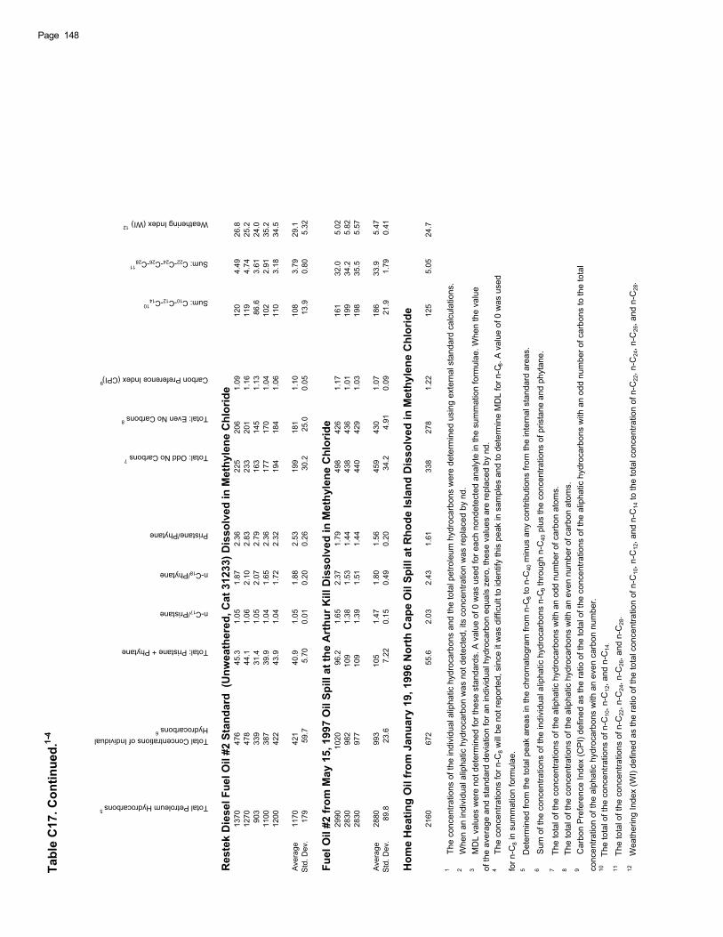
Tabl

e C

17. C

ontin

ued.

1-4

Total Petroleum Hydrocarbons 5

Total Concentrations of Individual Hydrocarbons

6

Total: Pristane + Phytane

n-C17/Pristane

n-C18/Phytane

Pristane/Phytane

Total: Odd No Carbons 7

Total: Even No Carbons 8

Carbon Preference Index (CPI)9

Sum: C10-C12-C1410

Sum: C22-C24-C26-C2811

Weathering Index (WI) 12

Res

tek

Die

sel F

uel O

il #2

Sta

ndar

d (U

nwea

ther

ed, C

at 3

1233

) Dis

solv

ed in

Met

hyle

ne C

hlor

ide

13

70

4

76

4

5.3

1.05

1.87

2.36

2

25

2

06

1.09

1

20

4.49

2

6.8

12

70

4

78

4

4.1

1.06

2.10

2.83

2

33

2

01

1.16

1

19

4.74

2

5.2

9

03

3

39

3

1.4

1.05

2.07

2.79

1

63

1

45

1.13

8

6.6

3.61

2

4.0

11

00

3

87

3

9.9

1.04

1.65

2.36

1

77

1

70

1.04

1

02

2.91

3

5.2

12

00

4

22

4

3.9

1.04

1.72

2.32

1

94

1

84

1.06

1

10

3.18

3

4.5

Ave

rage

11

70

4

21

4

0.9

1.05

1.88

2.53

1

99

1

81

1.10

1

08

3.79

2

9.1

Std

. Dev

.

179

59.

7

5.

70

0.

01

0.

20

0.

26

30.

2

25.

0

0.

05

13.

9

0.

80

5.

32

Fuel

Oil

#2 fr

om M

ay 1

5, 1

997

Oil

Spill

at t

he A

rthu

r Kill

Dis

solv

ed in

Met

hyle

ne C

hlor

ide

29

90

10

20

9

6.2

1.65

2.37

1.79

4

98

4

26

1.17

1

61

3

2.0

5.02

28

30

9

82

1

09

1.38

1.53

1.44

4

38

4

36

1.01

1

99

3

4.2

5.82

28

30

9

77

1

09

1.39

1.51

1.44

4

40

4

29

1.03

1

98

3

5.5

5.57

Ave

rage

28

80

9

93

1

05

1.47

1.80

1.56

4

59

4

30

1.07

1

86

3

3.9

5.47

Std

. Dev

.

89.

8

23.

6

7.

22

0.

15

0.

49

0.

20

34.

2

4.

91

0.

09

21.

9

1.

79

0.

41

Hom

e H

eatin

g O

il fr

om J

anua

ry 1

9, 1

996

Nor

th C

ape

Oil

Spill

at R

hode

Isla

nd D

isso

lved

in M

ethy

lene

Chl

orid

e

21

60

6

72

5

5.6

2.03

2.43

1.61

3

38

2

78

1.22

1

25

5.05

2

4.7

1

The

conc

entra

tions

of t

he in

divi

dual

alip

hatic

hyd

roca

rbon

s an

d th

e to

tal p

etro

leum

hyd

roca

rbon

s w

ere

dete

rmin

ed u

sing

ext

erna

l sta

ndar

d ca

lcul

atio

ns.

2

Whe

n an

indi

vidu

al a

lipha

tic h

ydro

carb

on w

as n

ot d

etec

ted,

its

conc

entra

tion

was

repl

aced

by

nd.

3

MD

L va

lues

wer

e no

t det

erm

ined

for t

hese

sta

ndar

ds. A

val

ue o

f 0 w

as u

sed

for e

ach

nond

etec

ted

anal

yte

in th

e su

mm

atio

n fo

rmul

ae. W

hen

the

valu

e of

the

aver

age

and

stan

dard

dev

iatio

n fo

r an

indi

vidu

al h

ydro

carb

on e

qual

s ze

ro, t

hese

val

ues

are

repl

aced

by

nd.

4

The

conc

entra

tions

for n

-C8 w

ill b

e no

t rep

orte

d, s

ince

it w

as d

iffic

ult t

o id

entif

y th

is p

eak

in s

ampl

es a

nd to

det

erm

ine

MD

L fo

r n-C

8. A

val

ue o

f 0 w

as u

sed

for n

-C8 i

n su

mm

atio

n fo

rmul

ae.

5

Det

erm

ined

from

the

tota

l pea

k ar

eas

in th

e ch

rom

atog

ram

from

n-C

8 to

n-C

40 m

inus

any

con

tribu

tions

from

the

inte

rnal

sta

ndar

d ar

eas.

6

Sum

of t

he c

once

ntra

tions

of t

he in

divi

dual

alip

hatic

hyd

roca

rbon

s n-

C 9 th

roug

h n-

C40

plu

s th

e co

ncen

tratio

ns o

f pris

tane

and

phy

tane

.7

Th

e to

tal o

f the

con

cent

ratio

ns o

f the

alip

hatic

hyd

roca

rbon

s w

ith a

n od

d nu

mbe

r of c

arbo

n at

oms.

8

The

tota

l of t

he c

once

ntra

tions

of t

he a

lipha

tic h

ydro

carb

ons

with

an

even

num

ber o

f car

bon

atom

s.9

C

arbo

n P

refe

renc

e In

dex

(CP

I) de

fined

as

the

ratio

of t

he to

tal o

f the

con

cent

ratio

ns o

f the

alip

hatic

hyd

roca

rbon

s w

ith a

n od

d nu

mbe

r of c

arbo

ns to

the

tota

lco

ncen

tratio

n of

the

alph

atic

hyd

roca

rbon

s w

ith a

n ev

en c

arbo

n nu

mbe

r.10

The

tota

l of t

he c

once

ntra

tions

of n

-C10

, n-C

12, a

nd n

-C14

.11

The

tota

l of t

he c

once

ntra

tions

of n

-C22

, n-C

24, n

-C26

, and

n-C

28.

12

Wea

ther

ing

Inde

x (W

I) de

fined

as

the

ratio

of t

he to

tal c

once

ntra

tion

of n

-C10

, n-C

12, a

nd n

-C14

to th

e to

tal c

once

ntra

tion

of n

-C22

, n-C

24, n

-C26

, and

n-C

28.

Page 148

149Page

APPENDIX D

INDIVIDUAL AND TOTAL PETROLEUM HYDROCARBON CONCENTRATIONS

Table D1. Individual hydrocarbon and total petroleum hydrocarbon concentrations for sediment taken from Old Placemarsh, a replanted site

Table D2. Individual hydrocarbon and total petroleum hydrocarbon concentrations for sediment taken from Con EdisonTower marsh, an unplanted site

Table D3. Individual hydrocarbon and total petroleum hydrocarbon concentrations for sediment cores taken from MillCreek marsh, a reference site

Table D4. Individual hydrocarbon concentrations for sediment surface skims taken from Sandy Hook Bay marsh, areference site

Table D5. Individual hydrocarbon and total petroleum hydrocarbon concentrations for ribbed mussels taken from OldPlace marsh, a replanted site

Table D6. Individual hydrocarbon and total petroleum hydrocarbon concentrations for ribbed mussels taken from ConEdison Tower marsh, an unplanted site

Table D7. Individual hydrocarbon and total petroleum hydrocarbon concentrations for ribbed mussels taken from SawMill North marsh, a replanted site

Table D8. Individual hydrocarbon and total petroleum hydrocarbon concentrations for ribbed mussels taken from SawMill South marsh, an unplanted site

Table D9. Individual hydrocarbon and total petroleum hydrocarbon concentrations for ribbed mussels taken from TuftsPoint marsh, a reference site

Table D10. Individual hydrocarbon and total petroleum hydrocarbon concentrations for ribbed mussels taken from MillCreek marsh, a reference site

Table D11. Individual hydrocarbon and total petroleum hydrocarbon concentrations for ribbed mussels taken fromSandy Hook marsh, a reference site

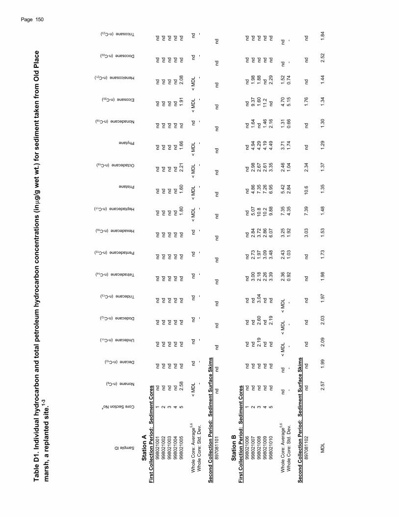
Tabl

e D

1. In

divi

dual

hyd

roca

rbon

and

tota

l pet

role

um h

ydro

carb

on c

once

ntra

tions

(in

g/g

wet

wt.)

for s

edim

ent t

aken

from

Old

Pla

ce

mar

sh, a

repl

ante

d si

te.1-

3

Sample ID

Core Section No4

Nonane (n-C9)

Decane (n-C10)

Undecane (n-C11)

Dodecane (n-C12)

Tridecane (n-C13)

Tetradecane (n-C14)

Pentadecane (n-C15)

Hexadecane (n-C16)

Heptadecane (n-C17)

Pristane

Octadecane (n-C18)

Phytane

Nonadecane (n-C19)

Eicosane (n-C20)

Heneicosane (n-C21)

Docosane (n-C22)

Tricosane (n-C23)

Stat

ion

AFi

rst C

olle

ctio

n Pe

riod:

Sed

imen

t Cor

es99

8021

001

1

nd

nd

nd

nd

nd

nd

nd

nd

nd

nd

nd

nd

nd

nd

nd

nd

nd

99

8021

002

2

nd

nd

nd

nd

nd

nd

nd

nd

nd

nd

nd

nd

nd

nd

nd

nd

nd

99

8021

003

3

nd

nd

nd

nd

nd

nd

nd

nd

nd

nd

nd

nd

nd

nd

nd

nd

nd

99

8021

004

4

nd

nd

nd

nd

nd

nd

nd

nd

nd

nd

nd

nd

nd

nd

nd

nd

nd

99

8021

005

5

2.

58

nd

nd

nd

nd

nd

nd

nd

1.

80

1.

60

2.

21

1.

66

nd

1.

91

2.

08

nd

nd

Who

le C

ore:

Ave

rage

5,6

<

MD

L

n

d

n

d

n

d

n

d

n

d

n

d

n

d

< M

DL

<

MD

L

< M

DL

<

MD

L

n

d

< M

DL

<

MD

L

n

d

n

d W

hole

Cor

e: S

td. D

ev.

-

-

-

-

-

-

-

-

-

-

-

-

-

-

-

-

-

Seco

nd C

olle

ctio

n Pe

riod:

Sed

imen

t Sur

face

Ski

ms

8970

8110

1nd

ndnd

ndnd

ndnd

ndnd

ndnd

ndnd

ndnd

ndnd

Stat

ion

BFi

rst C

olle

ctio

n Pe

riod:

Sed

imen

t Cor

es99

8021

006

1

nd

nd

nd

nd

nd

nd

nd

nd

nd

nd

nd

nd

nd

nd

nd

nd

nd

99

8021

007

2

nd

nd

nd

nd

nd

3.

00

2.

73

2.

84

5.

07

4.

86

2.

98

4.

94

1.

64

9.

37

1.

98

nd

nd

99

8021

008

3

nd

nd

2.

19

2.

60

3.

04

2.

18

1.

97

3.

72

10.

8

7.

35

2.

67

4.

29

nd

1.

60

1.

88

nd

nd

99

8021

009

4

nd

nd

nd

nd

nd

2.

26

3.

09

2.

86

10.

2

7.

26

2.

61

4.

19

1.

46

11.

2

nd

nd

nd

99

8021

010

5

nd

nd

nd

2.

19

nd

3.

39

3.

48

6.

07

9.

88

6.

95

3.

35

4.

49

2.

16

nd

2.

29

nd

nd

Who

le C

ore:

Ave

rage

5,6

n

d

nd

< M

DL

<

MD

L

< M

DL

2.36

2.43

3.25

7.35

5.42

2.46

3.71

1.31

4.70

1.52

n

d

nd

Who

le C

ore:

Std

. Dev

.

-

-

-

-

-

0.92

1.03

1.92

4.35

2.84

1.04

1.74

0.66

5.15

0.74

-

-

Seco

nd C

olle

ctio

n Pe

riod:

Sed

imen

t Sur

face

Ski

ms

8970

8110

2

nd

nd

nd

nd

nd

nd

nd

3.

03

7.

39

10.

6

2.

34

nd

nd

1.

76

nd

nd

nd

MD

L2.

571.

992.

092.

031.

971.

981.

731.

531.

481.

351.

371.

291.

301.

341.

442.

521.

84

Page 150

Tabl

e D

1. C

ontin

ued.

1,2

Sample ID

Core Section No4

Tetracosane (n-C24)

Pentacosane (n-C25)

Hexacosane (n-C26)

Heptacosane (n-C27)

Octacosane (n-C28)

Nonacosane (n-C29)

Triacontane (n-C30)

n-Hentriacontane (n-C31)

Dotriacontane (n-C32)

Tritriacontane (n-C33)

Tetratriacontane (n-C34)

Pentatriacontane (n-C35)

Hexatriacontane (n-C36)

Heptatriacontane (n-C37)

Octatriacontane (n-C38)

Nonatriacontane (n-C39)

Tetracontane (n-C40)

Stat

ion

AFi

rst C

olle

ctio

n Pe

riod:

Sed

imen

t Cor

es99

8021

001

1

nd

nd

nd

nd

nd

nd

nd

nd

nd

nd

nd

nd

nd

nd

nd

nd

nd

99

8021

002

2

nd

nd

nd

nd

nd

nd

nd

nd

nd

nd

nd

nd

nd

nd

nd

nd

nd

99

8021

003

3

nd

nd

nd

nd

nd

nd

nd

nd

nd

nd

nd

nd

nd

nd

nd

nd

nd

99

8021

004

4

nd

nd

nd

nd

nd

nd

nd

nd

nd

nd

nd

nd

nd

nd

nd

nd

nd

99

8021

005

5

nd

nd

nd

nd

nd

nd

nd

5.

64

2.

48

nd

nd

nd

1.

23

1.

09

1.

35

1.

34

1.

13

Who

le C

ore:

Ave

rage

5,6

ndnd

ndnd

ndnd

nd<

MD

L<

MD

Lnd

ndnd

< M

DL

< M

DL

< M

DL

< M

DL

< M

DL

Who

le C

ore:

Std

. Dev

.-

--

--

--

--

--

--

--

--

Seco

nd C

olle

ctio

n Pe

riod:

Sed

imen

t Sur

face

Ski

ms

8970

8110

1nd

ndnd

ndnd

ndnd

ndnd

ndnd

ndnd

ndnd

ndnd

Stat

ion

BFi

rst C

olle

ctio

n Pe

riod:

Sed

imen

t Cor

es99

8021

006

1

nd

nd

nd

nd

nd

nd

nd

4.

90

3.

27

11.

2

nd

nd

0.

84

nd

nd

nd

nd

99

8021

007

2

nd

nd

nd

nd

nd

nd

nd

nd

nd

nd

nd

nd

nd

nd

nd

nd

nd

99

8021

008

3

nd

nd

nd

nd

nd

nd

nd

nd

nd

nd

nd

nd

nd

nd

nd

nd

nd

99

8021

009

4

nd

nd

nd

nd

nd

nd

nd

3.

87

1.

69

nd

nd

2.

29

nd

nd

nd

nd

nd

99

8021

010

5

nd

nd

nd

nd

nd

nd

nd

2.

40

2.

02

nd

nd

nd

nd

nd

nd

nd

nd

Who

le C

ore:

Ave

rage

5,6

n

d

n

d

n

d

n

d

n

d

n

d

n

d

2.64

1.72

< M

DL

nd

<

MD

L

< M

DL

nd

nd

nd

nd

W

hole

Cor

e: S

td. D

ev.

-

-

-

-

-

-

-

1.73

1.02

-

-

-

-

-

-

-

-

Seco

nd C

olle

ctio

n Pe

riod:

Sed

imen

t Sur

face

Ski

ms

8970

8110

2nd

ndnd

ndnd

ndnd

ndnd

ndnd

ndnd

ndnd

ndnd

MD

L

1.

47

1.

69

1.

39

1.

96

1.

51

3.

13

1.

05

2.

03

1.

60

8.

25

0.

71

1.

25

0.

73

0.

68

0.

61

0.

53

0.

56

151Page

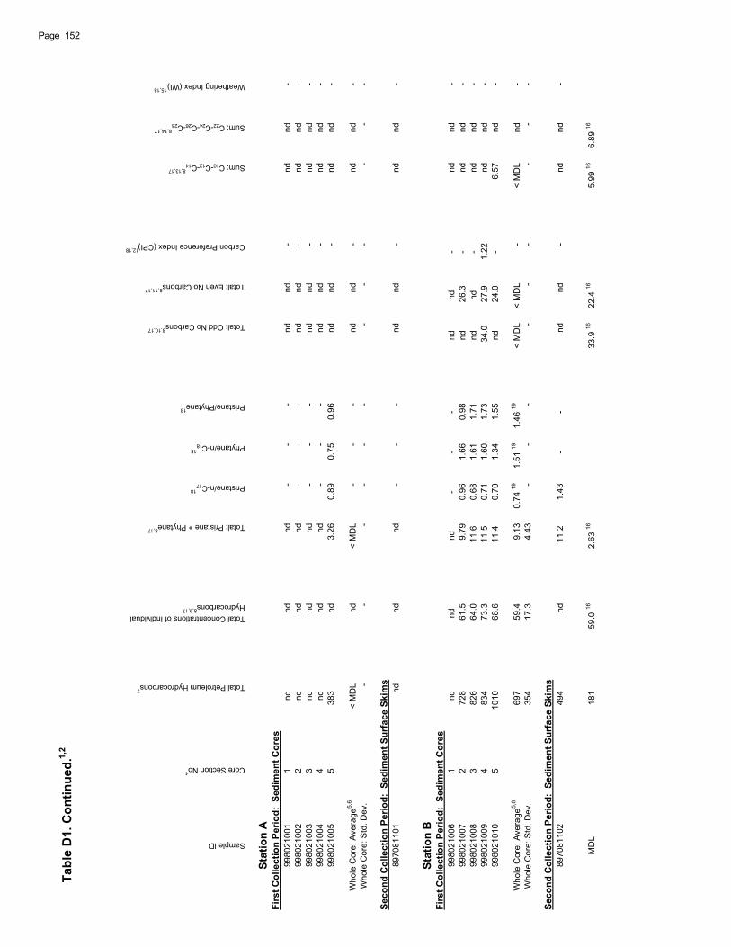
Tabl

e D

1. C

ontin

ued.

1,2

Sample ID

Core Section No4

Total Petroleum Hydrocarbons7

Total Concentrations of Individual Hydrocarbons

8,9,17

Total: Pristane + Phytane8,17

Pristane/n-C1718

Phytane/n-C1818

Pristane/Phytane18

Total: Odd No Carbons8,10,17

Total: Even No Carbons8,11,17

Carbon Preference Index (CPI)12,18

Sum: C10-C12-C148,13,17

Sum: C22-C24-C26-C288,14,17

Weathering Index (WI)15,18

Stat

ion

AFi

rst C

olle

ctio

n Pe

riod:

Sed

imen

t Cor

es99

8021

001

1

nd

ndnd

--

-nd

nd-

ndnd

-99

8021

002

2

nd

ndnd

--

-nd

nd-

ndnd

-99

8021

003

3

nd

ndnd

--

-nd

nd-

ndnd

-99

8021

004

4

nd

ndnd

--

-nd

nd-

ndnd

-99

8021

005

5

383

nd3.

260.

890.

750.

96nd

nd-

ndnd

-

Who

le C

ore:

Ave

rage

5,6

< M

DL

nd<

MD

L-

--

ndnd

-nd

nd-

Who

le C

ore:

Std

. Dev

.-

--

--

--

--

--

-

Seco

nd C

olle

ctio

n Pe

riod:

Sed

imen

t Sur

face

Ski

ms

8970

8110

1nd

ndnd

--

-nd

nd-

ndnd

-

Stat

ion

BFi

rst C

olle

ctio

n Pe

riod:

Sed

imen

t Cor

es99

8021

006

1

nd

nd

nd

-

-

-

nd

nd

-

nd

nd-

9980

2100

72

7

28

61

.5

9.

79

0.

96

1.

66

0.

98

nd

26.

3

-

nd

nd-

9980

2100

83

8

26

64

.0

11.

6

0.

68

1.

61

1.

71

nd

nd

-

nd

nd-

9980

2100

94

8

34

73

.3

11.

5

0.

71

1.

60

1.

73

34.

0

27.

9

1.

22nd

nd-

9980

2101

05

10

10

68

.6

11.

4

0.

70

1.

34

1.

55

nd

24.

0

-

6.

57nd

-

Who

le C

ore:

Ave

rage

5,6

6

97

59

.49.

130.

74 19

1.51

191.

4619

< M

DL

< M

DL

-<

MD

Lnd

-W

hole

Cor

e: S

td. D

ev.

3

54

17

.34.

43-

--

--

--

--

Seco

nd C

olle

ctio

n Pe

riod:

Sed

imen

t Sur

face

Ski

ms

8970

8110

2

494

nd

11.

2

1.

43

-

-

nd

nd-

ndnd

-

MD

L

181

5

9.0

162.

6316

33.9

1622

.416

5.99

166.

8916

Page 152

Tabl

e D

1. C

ontin

ued.

1-3

Sample ID

Core Section No4

Nonane (n-C9)

Decane (n-C10)

Undecane (n-C11)

Dodecane (n-C12)

Tridecane (n-C13)

Tetradecane (n-C14)

Pentadecane (n-C15)

Hexadecane (n-C16)

Heptadecane (n-C17)

Pristane

Octadecane (n-C18)

Phytane

Nonadecane (n-C19)

Eicosane (n-C20)

Heneicosane (n-C21)

Docosane (n-C22)

Tricosane (n-C23)

Stat

ion

CFi

rst C

olle

ctio

n Pe

riod:

Sed

imen

t Cor

es99

8021

011

1

nd

nd

nd

nd

nd

nd

nd

nd

nd

nd

nd

nd

1.

51

nd

nd

nd

nd

99

8021

012

2

nd

nd

nd

nd

nd

nd

nd

nd

1.

61

nd

nd

nd

nd

nd

nd

nd

nd

99

8021

013

3

nd

nd

nd

nd

nd

nd

nd

nd

nd

nd

nd

nd

nd

nd

nd

nd

nd

99

8021

014

4

nd

nd

nd

nd

nd

nd

nd

nd

nd

nd

nd

nd

nd

nd

nd

nd

nd

99

8021

015

5

nd

nd

nd

nd

nd

nd

nd

nd

1.

53

nd

nd

nd

nd

nd

nd

nd

nd

Who

le C

ore:

Ave

rage

5,6

n

d

n

d

n

d

n

d

n

d

n

d

n

d

n

d

< M

DL

nd

nd

nd

<

MD

L

n

d

n

d

n

d

n

d

Who

le C

ore:

Std

. Dev

.

-

-

-

-

-

-

-

-

-

-

-

-

-

-

-

-

-

Seco

nd C

olle

ctio

n Pe

riod:

Sed

imen

t Sur

face

Ski

ms

8970

8110

3

n

d

n

d

n

d

n

d

n

d

n

d

n

d

n

d

n

d

n

d

n

d

n

d

n

d

n

d

n

d

n

d

n

d

Stat

ion

DFi

rst C

olle

ctio

n Pe

riod:

Sed

imen

t Cor

es99

8021

016

1

nd

nd

nd

nd

nd

nd

nd

nd

nd

nd

nd

nd

nd

nd

nd

nd

nd

99

8021

017

2

nd

nd

nd

nd

nd

nd

nd

nd

nd

nd

nd

nd

nd

nd

nd

nd

nd

99

8021

018

3

nd

nd

2.

46

3.

46

3.

47

3.

25

3.

21

5.

98

11.

3

8.

21

4.

06

5.

20

nd

2.

54

2.

31

nd

nd

99

8021

019

4

nd

nd

12.

9

13.

8

5.

04

10.

1

11.

4

6.

57

15.

7

15.

8

23.

0

30.

6

15.

2

2.

86

3.

85

4.

27

3.

9899

8021

020

5

nd

nd

6.

48

5.

78

10.

8

13.

4

9.

05

20.

2

38.

1

31.

0

13.

9

19.

6

6.

08

31.

3

3.

97

2.

70

1.

94

Who

le C

ore:

Ave

rage

5,6

n

d

n

d

4.78

5.01

4.26

5.75

5.07

6.86

1

3.3

1

1.3

8.47

1

1.3

4.64

7.61

2.32

< M

DL

<

MD

L

Who

le C

ore:

Std

. Dev

.

-

-

5.

05

5.

28

4.

05

5.

69

4.

86

7.

96

15.

4

12.

7

9.

76

13.

3

6.

33

13.

3

1.

60

-

-

Seco

nd C

olle

ctio

n Pe

riod:

Sed

imen

t Sur

face

Ski

ms

8970

8110

4nd

ndnd

ndnd

ndnd

ndnd

ndnd

ndnd

ndnd

ndnd

MD

L2.

571.

992.

092.

031.

971.

981.

731.

531.

481.

351.

371.

291.

301.

341.

442.

521.

84

153Page

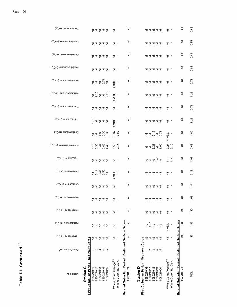
Tabl

e D

1. C

ontin

ued.

1,2

Sample ID

Core Section No4

Tetracosane (n-C24)

Pentacosane (n-C25)

Hexacosane (n-C26)

Heptacosane (n-C27)

Octacosane (n-C28)

Nonacosane (n-C29)

Triacontane (n-C30)

n-Hentriacontane (n-C31)

Dotriacontane (n-C32)

Tritriacontane (n-C33)

Tetratriacontane (n-C34)

Pentatriacontane (n-C35)

Hexatriacontane (n-C36)

Heptatriacontane (n-C37)

Octatriacontane (n-C38)

Nonatriacontane (n-C39)

Tetracontane (n-C40)

Stat

ion

CFi

rst C

olle

ctio

n Pe

riod:

Sed

imen

t Cor

es99

8021

011

1

nd

nd

nd

nd

nd

nd

nd

6.

13

nd

10.

3

nd

nd

nd

nd

nd

nd

nd

99

8021

012

2

nd

nd

nd

nd

nd

3.

14

nd

5.

36

nd

nd

nd

1.

26

nd

nd

nd

nd

nd

99

8021

013

3

nd

nd

nd

nd

nd

3.

47

nd

6.

44

4.

80

nd

nd

nd

nd

nd

nd

nd

nd

99

8021

014

4

nd

nd

nd

nd

nd

3.

50

nd

5.

43

6.

33

nd

nd

nd

0.

74

nd

nd

nd

nd

99

8021

015

5

nd

nd

nd

nd

nd

nd

nd

4.

46

6.

35

nd

nd

2.

23

nd

nd

nd

nd

nd

Who

le C

ore:

Ave

rage

5,6

n

d

n

d

n

d

n

d

n

d

< M

DL

nd

5.

56

3.

82 <

MD

L

n

d

< M

DL

<

MD

L

n

d

n

d

n

d

n

d

Who

le C

ore:

Std

. Dev

.

-

-

-

-

-

-

-

0.

77

2.

82

-

-

-

-

-

-

-

-

Seco

nd C

olle

ctio

n Pe

riod:

Sed

imen

t Sur

face

Ski

ms

8970

8110

3nd

ndnd

ndnd

ndnd

ndnd

ndnd

ndnd

ndnd

ndnd

Stat

ion

DFi

rst C

olle

ctio

n Pe

riod:

Sed

imen

t Cor

es99

8021

016

1

nd

nd

nd

nd

nd

nd

nd

nd

nd

nd

nd

nd

nd

nd

nd

nd

nd

99

8021

017

2

nd

4.

11

nd

nd

nd

nd

nd

nd

nd

nd

nd

nd

nd

nd

nd

nd

nd

99

8021

018

3

nd

nd

nd

nd

nd

nd

nd

6.

33

2.

15

nd

nd

nd

nd

nd

nd

nd

nd

99

8021

019

4

nd

nd

nd

nd

nd

nd

3.

46

nd

nd

nd

nd

nd

nd

nd

nd

nd

nd

99

8021

020

5

nd

nd

nd

nd

nd

nd

nd

6.

99

2.

78

nd

nd

nd

nd

nd

nd

nd

nd

Who

le C

ore:

Ave

rage

5,6

n

d

<

MD

L

n

d

n

d

n

d

n

d

1.11

3.27

< M

DL

nd

nd

nd

nd

nd

nd

nd

nd

W

hole

Cor

e: S

td. D

ev.

-

-

-

-

-

-

1.31

3.10

-

-

-

-

-

-

-

-

-

Seco

nd C

olle

ctio

n Pe

riod:

Sed

imen

t Sur

face

Ski

ms

8970

8110

4nd

ndnd

ndnd

ndnd

ndnd

ndnd

ndnd

ndnd

ndnd

MD

L1.

471.

691.

391.

961.

513.

131.

052.

031.

608.

250.

711.

250.

730.

680.

610.

530.

56

Page 154

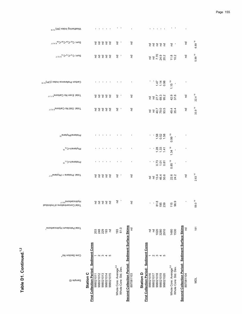
Tabl

e D

1. C

ontin

ued.

1,2

Sample ID

Core Section No4

Total Petroleum Hydrocarbons7

Total Concentrations of Individual Hydrocarbons

8,9,17

Total: Pristane + Phytane8,17

Pristane/n-C1718

Phytane/n-C1818

Pristane/Phytane18

Total: Odd No Carbons8,10,17

Total: Even No Carbons8,11,17

Carbon Preference Index (CPI)12,18

Sum: C10-C12-C148,13,17

Sum: C22-C24-C26-C288,14,17

Weathering Index (WI)15,18

Stat

ion

CFi

rst C

olle

ctio

n Pe

riod:

Sed

imen

t Cor

es99

8021

011

1

203

nd

nd

-

-

-

nd

nd

-

nd

nd

-

9980

2101

22

2

48

n

d

n

d

-

-

-

n

d

n

d

-

n

d

n

d

-

99

8021

013

3

229

nd

nd

-

-

-

nd

nd

-

nd

nd

-

9980

2101

44

1

93

n

d

n

d

-

-

-

n

d

n

d

-

n

d

n

d

-

99

8021

015

5

nd

nd

nd

-

-

-

nd

nd

-

nd

nd

-

Who

le C

ore:

Ave

rage

5,6

1

93

n

d

n

d

-

-

-

n

d

n

d

-

n

d

n

d -

Who

le C

ore:

Std

. Dev

.

61.

0 -

-

-

-

-

-

-

-

-

-

-

Seco

nd C

olle

ctio

n Pe

riod:

Sed

imen

t Sur

face

Ski

ms

8970

8110

3

n

d

n

d

n

d

-

-

-

n

d

n

d

-

n

d

n

d

-

Stat

ion

DFi

rst C

olle

ctio

n Pe

riod:

Sed

imen

t Cor

es99

8021

016

1

nd

-

nd

-

-

-

nd

nd

-

n

d

n

d

-

9980

2101

72

n

d

-

n

d

-

-

-

n

d

n

d

-

nd

nd

-

99

8021

018

3

1020

8

1.8

1

3.4

0.73

1.28

1.58

4

0.7

2

7.7

1.47

7.70

n

d

-

9980

2101

94

32

80

195

4

6.4

1.01

1.33

0.52

7

9.0

6

9.3

1.14

2

4.9

n

d

-

9980

2102

05

29

10

239

5

0.6

0.81

1.41

1.58

9

3.5

9

5.2

0.98

2

0.2

n

d

-

Who

le C

ore:

Ave

rage

5,6

14

80

115

2

2.6

0

.85

19

1.3

4 19

0

.99

19

49.

4

42.

9

1.1

5 19

1

1.8

n

d

-W

hole

Cor

e: S

td. D

ev.

15

30

96.

9

24.

2

-

-

-

35.

4

37.

6

-

10.

2

-

-

Seco

nd C

olle

ctio

n Pe

riod:

Sed

imen

t Sur

face

Ski

ms

8970

8110

4

n

d

-

n

d

-

-

-

n

d

n

d

-

n

d

n

d

-

MD

L18

159

.016

2.63

1633

.916

22.4

165.

9916

6.89

16

155Page

Tabl

e D

1. C

ontin

ued.

Foot

note

s:

1

The

conc

entra

tions

of t

he in

divi

dual

alip

hatic

hyd

roca

rbon

s an

d th

e to

tal p

etro

leum

hyd

roca

rbon

s w

ere

dete

rmin

ed u

sing

ext

erna

l sta

ndar

d ca

lcul

atio

ns.

2

Whe

n an

indi

vidu

al a

lipha

tic h

ydro

carb

on w

as n

ot d

etec

ted,

its

conc

entra

tion

was

repl

aced

by

nd.

3

The

conc

entra

tions

for n

-C8 w

ill b

e no

t rep

orte

d, s

ince

it w

as d

iffic

ult t

o id

entif

y th

is p

eak

in s

ampl

es a

nd to

det

erm

ine

MD

L fo

r n-C

8. A

val

ue o

f 0 w

as u

sed

for e

ach

nond

etec

ted

anal

yte

in s

umm

atio

n fo

rmul

ae.

4

For t

he s

edim

ent c

ores

, the

se n

umbe

rs re

pres

ent t

he d

epth

s in

to e

ach

core

: 1 -

dept

h 0

to 1

cm

; 2 -

dept

h 1

to 2

cm

; 3 -

dept

h 2

to 3

cm

; 4 -

dept

h 3

to 4

cm

;an

d, 5

- de

pth

4 to

5 c

m. F

or s

urfa

ce s

kim

s, th

e to

pmos

t 1 c

m la

yer i

s re

mov

ed fr

om th

e se

dim

ent s

urfa

ce.

5 T

he W

hole

Cor

e A

vera

ge a

nd S

tand

ard

Dev

iatio

n is

cal

cula

ted

usin

g th

e co

ncen

tratio

ns fo

r eac

h an

alyt

e ov

er a

ll co

re s

ectio

ns.

6

If al

l con

cent

ratio

ns a

re n

d, th

e av

erag

e is

repl

aced

with

nd.

Whe

n th

ere

is a

t lea

st o

ne n

umbe

r in

the

data

set

to b

e av

erag

ed, e

ach

nd is

repl

aced

w

ith 1

/2*M

DL,

and

an

aver

age

is c

alcu

late

d. If

this

num

eric

val

ue is

less

than

the

MD

L, th

e av

erag

e is

repl

aced

by

< M

DL;

oth

erw

ise,

the

aver

age

is th

eca

lcul

ated

val

ue. W

hen

a nu

mer

ic v

alue

is fo

und

for t

he a

vera

ge, t

he s

tand

ard

devi

atio

n is

then

det

erm

ined

usi

ng th

e sa

me

num

ber s

et u

sed

to c

alcu

late

the

aver

age.

7

Det

erm

ined

from

the

tota

l pea

k ar

eas

in th

e ch

rom

atog

ram

from

n-C

8 to

n-C

40 m

inus

any

con

tribu

tions

from

the

inte

rnal

sta

ndar

d ar

eas.

8 T

hese

form

ulae

use

1/2

MD

L va

lues

for e

ach

anal

yte

not d

etec

ted.

9 S

um o

f the

con

cent

ratio

ns o

f the

indi

vidu

al a

lipha

tic h

ydro

carb

ons

n-C

9 thr

ough

n-C

40 p

lus

the

conc

entra

tions

of p

rista

ne a

nd p

hyta

ne.

10 T

he to

tal o

f the

con

cent

ratio

ns o

f the

alip

hatic

hyd

roca

rbon

s w

ith a

n od

d nu

mbe

r of c

arbo

n at

oms.

11 T

he to

tal o

f the

con

cent

ratio

ns o

f the

alip

hatic

hyd

roca

rbon

s w

ith a

n ev

en n

umbe

r of c

arbo

n at

oms.

The

con

tribu

tion

of n

-C8 i

s no

t inc

lude

d in

the

tota

l.12

C

arbo

n P

refe

renc

e In

dex

(CP

I) de

fined

as

the

ratio

of t

he to

tal o

f the

con

cent

ratio

ns o

f the

alip

hatic

hyd

roca

rbon

s w

ith a

n od

d nu

mbe

r of c

arbo

ns to

the

tota

l con

cent

ratio

n of

the

alph

atic

hyd

roca

rbon

s w

ith a

n ev

en c

arbo

n nu

mbe

r.13

The

tota

l of t

he c

once

ntra

tions

of n

-C10

, n-C

12, a

nd n

-C14

.14

The

tota

l of t

he c

once

ntra

tions

of n

-C22

, n-C

24, n

-C26

, and

n-C

28.

15

Wea

ther

ing

Inde

x (W

I) is

def

ined

as

the

ratio

of t

he to

tal c

once

ntra

tion

of n

-C10

, n-C

12, a

nd n

-C14

to th

e to

tal c

once

ntra

tion

of n

-C22

, n-C

24, n

-C26

, and

n-C

28.

16

The

se M

DL

valu

es a

re c

alcu

late

d w

ith th

e sa

me

sum

mat

ion

form

ulae

as

the

sam

ples

usi

ng th

e in

divi

dual

hyd

roca

rbon

MD

L va

lues

.17

T

he s

umm

atio

n to

tals

for t

he s

ampl

es a

re c

ompa

red

with

cal

cula

ted

MD

L va

lues

obt

aine

d us

ing

the

sam

e su

mm

atio

n fo

rmul

ae a

s th

e sa

mpl

es.

Whe

n th

ese

sam

ple

tota

ls w

ere

less

than

the

tota

l MD

L, it

s va

lue

was

repl

aced

by

nd. T

he a

vera

ges

and

stan

dard

dev

iatio

ns fo

r the

tota

ls w

ere

treat

ed in

the

sam

e w

ay a

s th

e in

divi

dual

hyd

roca

rbon

s; s

ee fo

otno

te 6

.18

N

umer

ical

val

ues

of th

e C

PI,

WI,

and

the

ratio

s: p

rista

ne/n

-C17

, phy

tane

/n-C

18, a

nd p

rista

ne/p

hyta

ne, w

ill b

e ca

lcul

ated

onl

y w

hen

the

defin

ed q

uant

ityfo

r eac

h in

dex

or ra

tio h

as a

num

eric

val

ue.

19

The

se re

sults

are

not

true

ave

rage

s, in

stea

d th

ey a

re th

e ra

tios

of th

e av

erag

es o

f the

def

ined

qua

ntiti

es, i

f the

se a

vera

ges

exis

t.

Page 156

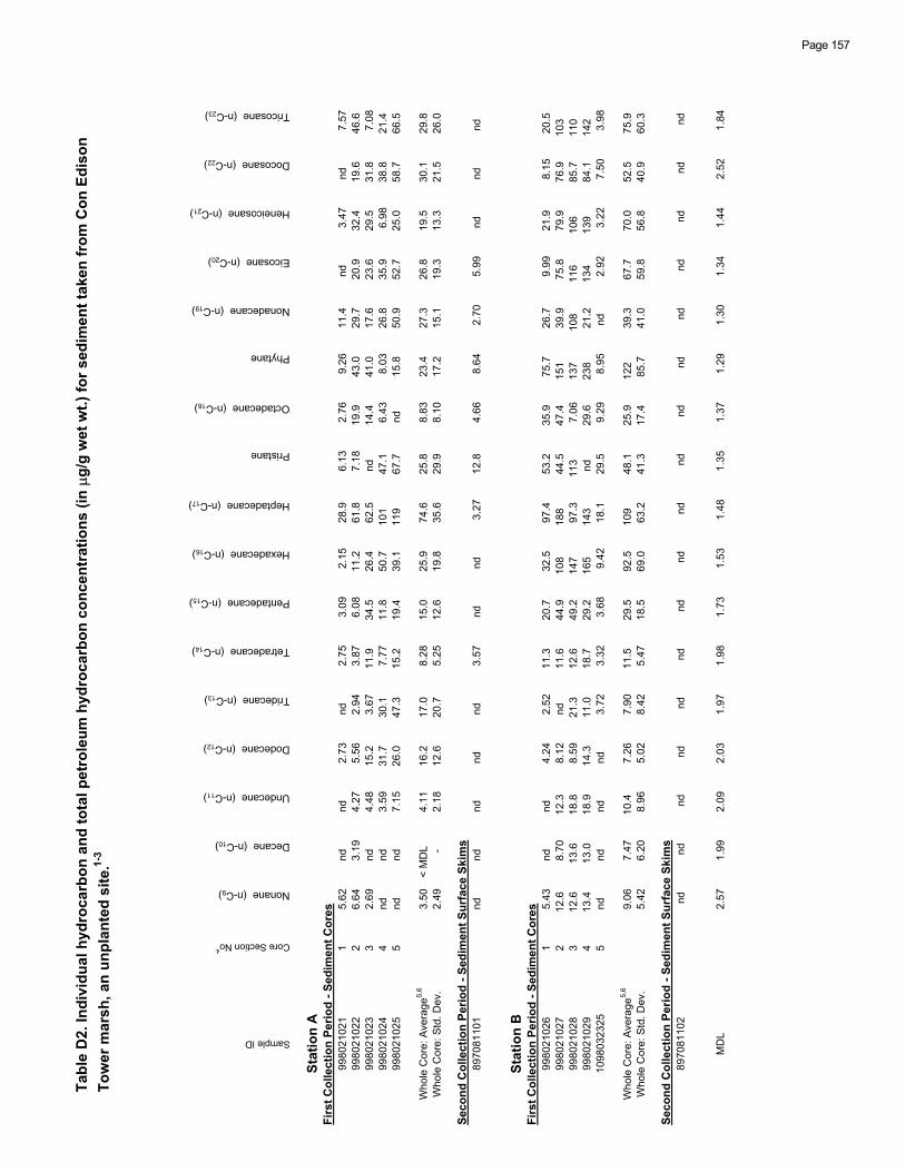
Tabl

e D

2. In

divi

dual

hyd

roca

rbon

and

tota

l pet

role

um h

ydro

carb

on c

once

ntra

tions

(in

g/g

wet

wt.)

for s

edim

ent t

aken

from

Con

Edi

son

Tow

er m

arsh

, an

unpl

ante

d si

te.1-

3

Sample ID

Core Section No4

Nonane (n-C9)

Decane (n-C10)

Undecane (n-C11)

Dodecane (n-C12)

Tridecane (n-C13)

Tetradecane (n-C14)

Pentadecane (n-C15)

Hexadecane (n-C16)

Heptadecane (n-C17)

Pristane

Octadecane (n-C18)

Phytane

Nonadecane (n-C19)

Eicosane (n-C20)

Heneicosane (n-C21)

Docosane (n-C22)

Tricosane (n-C23)

Stat

ion

AFi

rst C

olle

ctio

n Pe

riod

- Sed

imen

t Cor

es99

8021

021

1

5.

62

nd

nd

2.

73

nd

2.

75

3.

09

2.

15

28.

9

6.

13

2.

76

9.

26

11.

4

nd

3.

47

nd

7.

5799

8021

022

2

6.

64

3.

19

4.

27

5.

56

2.

94

3.

87

6.

08

11.

2

61.

8

7.

18

19.

9

43.

0

29.

7

20.

9

32.

4

19.

6

46.

6 99

8021

023

3

2.

69

nd

4.

48

15.

2

3.

67

11.

9

34.

5

26.

4

62.

5

nd

14.

4

41.

0

17.

6

23.

6

29.

5

31.

8

7.

0899

8021

024

4

nd

nd

3.

59

31.

7

30.

1

7.

77

11.

8

50.

7

101

47.

1

6.

43

8.

03

26.

8

35.

9

6.

98

38.

8

21.

4 99

8021

025

5

nd

nd

7.

15

26.

0

47.

3

15.

2

19.

4

39.

1

119

67.

7

nd

15.

8

50.

9

52.

7

25.

0

58.

7

66.

5

Who

le C

ore:

Ave

rage

5,6

3.50

< M

DL

4.

11

16.

2

17.

0

8.

28

15.

0

25.

9

74.

6

25.

8

8.

83

23.

4

27.

3

26.

8

19.

5

30.

1

29.

8 W

hole

Cor

e: S

td. D

ev.

2.49

-

2.18

1

2.6

2

0.7

5.25

1

2.6

1

9.8

3

5.6

2

9.9

8.10

1

7.2

1

5.1

1

9.3

1

3.3

2

1.5

2

6.0

Seco

nd C

olle

ctio

n Pe

riod

- Sed

imen

t Sur

face

Ski

ms

8970

8110

1

nd

nd

nd

nd

nd

3.

57

nd

nd

3.

27

12.

8

4.

66

8.

64

2.

70

5.

99

nd

nd

nd

Stat

ion

BFi

rst C

olle

ctio

n Pe

riod

- Sed

imen

t Cor

es99

8021

026

1

5.

43

nd

nd

4.

24

2.

52

11.

3

20.

7

32.

5

97.

4

53.

2

35.

9

75.

7

26.

7

9.

99

21.

9

8.

15

20.

5 99

8021

027

2

12.

6

8.

70

12.

3

8.

12

nd

11.

6

44.

9

108

188

44.

5

47.

4

151

39.

9

75.

8

79.

9

76.

9

103

99

8021

028

3

12.

6

13.

6

18.

8

8.

59

21.

3

12.

6

49.

2

147

97.

3

113

7.

06

137

108

116

106

85.

7

110

99

8021

029

4

13.

4

13.

0

18.

9

14.

3

11.

0

18.

7

29.

2

165

143

nd

29.

6

238

21.

2

134

139

84.

1

142

10

9803

2325

5

nd

nd

nd

nd

3.

72

3.

32

3.

68

9.

42

18.

1

29.

5

9.

29

8.

95

nd

2.

92

3.

22

7.

50

3.

98

Who

le C

ore:

Ave

rage

5,6

9.06

7.47

1

0.4

7.26

7.90

1

1.5

2

9.5

9

2.5

1

09

4

8.1

2

5.9

1

22

3

9.3

6

7.7

7

0.0

5

2.5

7

5.9

Who

le C

ore:

Std

. Dev

.

5.

42

6.

20

8.

96

5.

02

8.

42

5.

47

18.

5

69.

0

63.

2

41.

3

17.

4

85.

7

41.

0

59.

8

56.

8

40.

9

60.

3

Seco

nd C

olle

ctio

n Pe

riod

- Sed

imen

t Sur

face

Ski

ms

8970

8110

2

n

d

n

d

n

d

n

d

n

d

n

d

n

d

n

d

n

d

n

d

n

d

n

d

n

d

n

d

n

d

n

d

n

d

MD

L

2.

57

1.

99

2.

09

2.

03

1.

97

1.

98

1.

73

1.

53

1.

48

1.

35

1.

37

1.

29

1.

30

1.

34

1.

44

2.

52

1.

84

Page 157

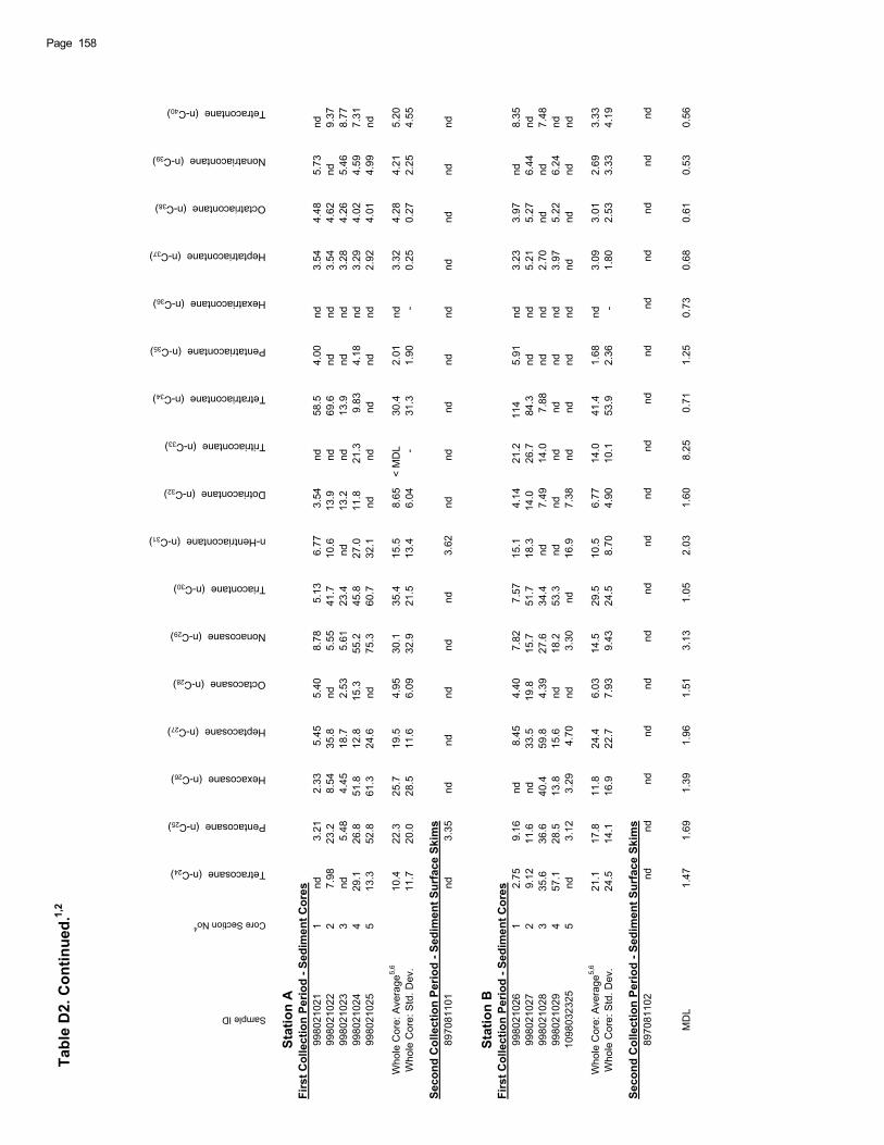
Tabl

e D

2. C

ontin

ued.

1,2

Sample ID

Core Section No4

Tetracosane (n-C24)

Pentacosane (n-C25)

Hexacosane (n-C26)

Heptacosane (n-C27)

Octacosane (n-C28)

Nonacosane (n-C29)

Triacontane (n-C30)

n-Hentriacontane (n-C31)

Dotriacontane (n-C32)

Tritriacontane (n-C33)

Tetratriacontane (n-C34)

Pentatriacontane (n-C35)

Hexatriacontane (n-C36)

Heptatriacontane (n-C37)

Octatriacontane (n-C38)

Nonatriacontane (n-C39)

Tetracontane (n-C40)

Stat

ion

AFi

rst C

olle

ctio

n Pe

riod

- Sed

imen

t Cor

es99

8021

021

1

nd

3.

21

2.

33

5.

45

5.

40

8.

78

5.

13

6.

77

3.

54

nd

58.

5

4.

00

nd

3.

54

4.

48

5.

73

nd

99

8021

022

2

7.

98

23.

2

8.

54

35.

8

nd

5.

55

41.

7

10.

6

13.

9

nd

69.

6

nd

nd

3.

54

4.

62

nd

9.

3799

8021

023

3

nd

5.

48

4.

45

18.

7

2.

53

5.

61

23.

4

nd

13.

2

nd

13.

9

nd

nd

3.

28

4.

26

5.

46

8.

7799

8021

024

4

29.

1

26.

8

51.

8

12.

8

15.

3

55.

2

45.

8

27.

0

11.

8

21.

3

9.

83

4.

18

nd

3.

29

4.

02

4.

59

7.

3199

8021

025

5

13.

3

52.

8

61.

3

24.

6

nd

75.

3

60.

7

32.

1

nd

nd

nd

nd

nd

2.

92

4.

01

4.

99

nd

Who

le C

ore:

Ave

rage

5,6

1

0.4

2

2.3

2

5.7

1

9.5

4.95

3

0.1

3

5.4

1

5.5

8.65

< M

DL

30.

4

2.

01

nd

3.

32

4.

28

4.

21

5.

20W

hole

Cor

e: S

td. D

ev.

1

1.7

2

0.0

2

8.5

1

1.6

6.09

3

2.9

2

1.5

1

3.4

6.04

-

3

1.3

1.90

-

0.25

0.27

2.25

4.55

Seco

nd C

olle

ctio

n Pe

riod

- Sed

imen

t Sur

face

Ski

ms

8970

8110

1

nd

3.

35

nd

nd

nd

nd

nd

3.

62

nd

nd

nd

nd

nd

nd

nd

nd

nd

Stat

ion

BFi

rst C

olle

ctio

n Pe

riod

- Sed

imen

t Cor

es99

8021

026

1

2.

75

9.

16

nd

8.

45

4.

40

7.

82

7.

57

15.

1

4.

14

21.

2

114

5.

91

nd

3.

23

3.

97

nd

8.

3599

8021

027

2

9.

12

11.

6

nd

33.

5

19.

8

15.

7

51.

7

18.

3

14.

0

26.

7

84.

3

nd

nd

5.

21

5.

27

6.

44

nd

99

8021

028

3

35.

6

36.

6

40.

4

59.

8

4.

39

27.

6

34.

4

nd

7.

49

14.

0

7.

88

nd

nd

2.

70

nd

nd

7.

4899

8021

029

4

57.

1

28.

5

13.

8

15.

6

nd

18.

2

53.

3

nd

nd

nd

nd

nd

nd

3.

97

5.

22

6.

24

nd

10

9803

2325

5

nd

3.

12

3.

29

4.

70

nd

3.

30

nd

16.

9

7.

38

nd

nd

nd

nd

nd

nd

nd

nd

Who

le C

ore:

Ave

rage

5,6

2

1.1

1

7.8

1

1.8

2

4.4

6.03

1

4.5

2

9.5

1

0.5

6.77

1

4.0

4

1.4

1.68

n

d

3.09

3.01

2.69

3.33

Who

le C

ore:

Std

. Dev

.

24.

5

14.

1

16.

9

22.

7

7.

93

9.

43

24.

5

8.

70

4.

90

10.

1

53.

9

2.

36

-

1.

80

2.

53

3.

33

4.

19

Seco

nd C

olle

ctio

n Pe

riod

- Sed

imen

t Sur

face

Ski

ms

8970

8110

2nd

ndnd

ndnd

ndnd

ndnd

ndnd

ndnd

ndnd

ndnd

MD

L1.

471.

691.

391.

961.

513.

131.

052.

031.

608.

250.

711.

250.

730.

680.

610.

530.

56

Page 158

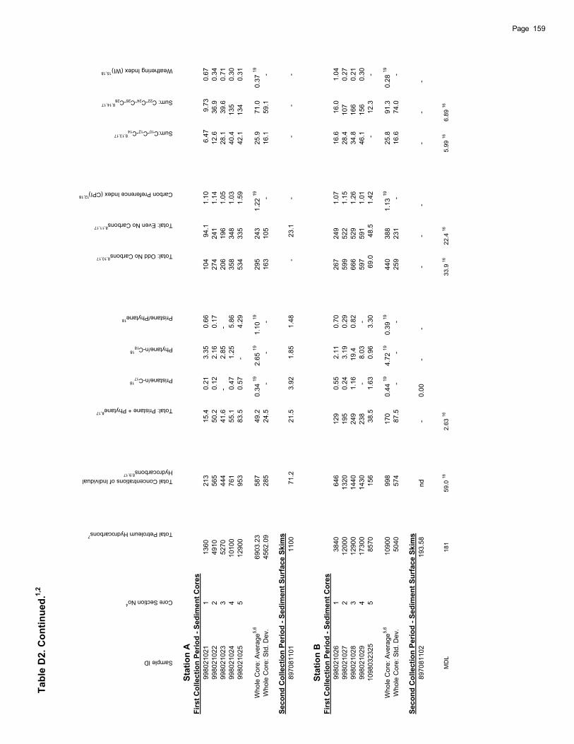
Tabl

e D

2. C

ontin

ued.

1,2

Sample ID

Core Section No4

Total Petroleum Hydrocarbons7

Total Concentrations of Individual Hydrocarbons

8,9,17

Total: Pristane + Phytane8,17

Pristane/n-C1718

Phytane/n-C1818

Pristane/Phytane18

Total: Odd No Carbons8,10,17

Total: Even No Carbons8,11,17

Carbon Preference Index (CPI)12,18

Sum:C10-C12-C148,13,17

Sum: C22-C24-C26-C288,14,17

Weathering Index (WI)15,18

Stat

ion

AFi

rst C

olle

ctio

n Pe

riod

- Sed

imen

t Cor

es99

8021

021

1

1360

213

15.

4

0.

21

3.

35

0.

66

104

94.

1

1.

10

6.

47

9.

73

0.

6799

8021

022

2

4910

565

50.

2

0.

12

2.

16

0.

17

274

241

1.

14

12.

6

36.

9

0.

3499

8021

023

3

5270

444

41.

6

-

2.85

-

206

196

1.

05

28.

1

39.

6

0.

7199

8021

024

4 1

0100

761

55.

1

0.

47

1.

25

5.

86

358

348

1.

03

40.

4

135

0.

3099

8021

025

5 1

2900

953

83.

5

0.

57

-

4.29

5

34

3

35

1.59

4

2.1

1

34

0.31

Who

le C

ore:

Ave

rage

5,6

6903

.23

5

87

4

9.2

0

.34

19

2.6

5 19

1

.10

19

295

243

1.2

2 19

2

5.9

7

1.0

0

.37

19

Who

le C

ore:

Std

. Dev

.45

62.0

9

285

24.

5

-

-

-

163

105

-

16.

1

59.

1

-

Seco

nd C

olle

ctio

n Pe

riod

- Sed

imen

t Sur

face

Ski

ms

8970

8110

1

1100

71.

2

21.

5

3.

92

1.

85

1.

48

-

23.

1

-

-

-

-

Stat

ion

BFi

rst C

olle

ctio

n Pe

riod

- Sed

imen

t Cor

es99

8021

026

1

3840

646

129

0.

55

2.

11

0.

70

267

249

1.

07

16.

6

16.

0

1.

0499

8021

027

2 1

2000

1320

195

0.

24

3.

19

0.

29

599

522

1.

15

28.

4

107

0.

2799

8021

028

3 1

2900

1440

249

1.

16

19.

4

0.

82

666

529

1.

26

34.

8

166

0.

2199

8021

029

4 1

7300

1430

238

-

8.

03

-

597

591

1.

01

46.

1

156

0.

3010

9803

2325

5

8570

156

38.

5

1.

63

0.

96

3.

30

69.

0

48.

5

1.

42

-

12.

3

-

Who

le C

ore:

Ave

rage

5,6

109

00

9

98

1

70

0

.44

19

4.7

2 19

0

.39

19

440

388

1.1

3 19

2

5.8

9

1.3

0

.28

19

Who

le C

ore:

Std

. Dev

.

5040

574

87.

5

-

-

-

259

231

-

16.

6

74.

0

-

Seco

nd C

olle

ctio

n Pe

riod

- Sed

imen

t Sur

face

Ski

ms

8970

8110

219

3.58

nd-

0.00

--

--

--

--

MD

L18

159

.016

2.63

1633

.916

22.4

165.

9916

6.89

16

159Page

Tabl

e D

2. C

ontin

ued.

1-3

Sample ID

Core Section No4

Nonane (n-C9)

Decane (n-C10)

Undecane (n-C11)

Dodecane (n-C12)

Tridecane (n-C13)

Tetradecane (n-C14)

Pentadecane (n-C15)

Hexadecane (n-C16)

Heptadecane (n-C17)

Pristane

Octadecane (n-C18)

Phytane

Nonadecane (n-C19)

Eicosane (n-C20)

Heneicosane (n-C21)

Docosane (n-C22)

Tricosane (n-C23)

Stat

ion

CFi

rst C

olle

ctio

n Pe

riod

- Sed

imen

t Cor

es11

9808

2510

1

nd

nd

nd

nd

nd

nd

nd

nd

5.

30

nd

nd

nd

nd

nd

nd

nd

nd

11

9808

2511

2

nd

nd

nd

nd

nd

nd

nd

nd

2.

11

nd

nd

nd

nd

nd

nd

nd

nd

11

9808

2512

3

nd

nd

nd

nd

nd

nd

nd

2.

26

8.

18

nd

nd

7.

43

1.

55

5.

71

6.

80

5.

66

2.

0311

9808

2513

4

nd

nd

nd

nd

nd

nd

2.

05

39.

2

51.

2

nd

7.

27

63.

2

25.

8

52.

5

36.

4

31.

5

22.

5 11

9808

2514

5

nd

nd

3.

35

nd

nd

12.

6

6.

96

15.

2

71.

6

nd

13.

0

100

44.

7

118

60.

4

56.

8

25.

9

Who

le C

ore:

Ave

rage

5,6

n

d

n

d

< M

DL

nd

nd

3.

31

2.

32

11.

6

27.

7

nd

4.

47

34.

4

14.

7

35.

5

21.

0

19.

3

10.

5 W

hole

Cor

e: S

td. D

ev.

-

-

-

-

-

5.20

2.65

1

6.6

3

1.7

-

5.57

4

5.1

1

9.9

5

0.9

2

6.5

2

4.5

1

2.6

Seco

nd C

olle

ctio

n Pe

riod

- Sed

imen

t Sur

face

Ski

ms

8970

8110

3

nd

nd

nd

nd

nd

nd

2.

77

nd

7.

08

nd

nd

nd

nd

nd

nd

nd

nd

Stat

ion

DFi

rst C

olle

ctio

n Pe

riod

- Sed

imen

t Cor

es11

9808

2505

1

nd

nd

nd

nd

nd

nd

nd

3.

35

2.

56

18.

9

nd

nd

nd

nd

nd

nd

nd

11

9808

2506

2

nd

nd

nd

8.

33

nd

2.

76

37.

7

15.

3

52.

8

8.

69

28.

6

44.

2

nd

24.

0

22.

9

24.

4

nd

11

9808

2507

3

nd

2.

70

6.

80

nd

7.

78

10.

0

9.

85

6.

97

52.

8

nd

nd

50.

3

1.

95

28.

8

5.

07

37.

6

7.

2211

9808

2508

4

3.

18

12.

7

9.

58

nd

8.

75

11.

8

15.

2

56.

5

73.

9

nd

nd

96.

0

3.

65

nd

62.

4

33.

1

9.

0911

9808

2509

5

4.

34

5.

13

10.

4

nd

11.

3

14.

9

17.

2

62.

3

102

117

4.

17

182

15.

3

43.

6

54.

8

10.

2

2.

94

Who

le C

ore:

Ave

rage

5,6

<

MD

L

4.51

5.77

2.48

5.97

8.10

1

6.2

2

8.9

5

6.8

2

9.2

6.96

7

4.7

4.44

1

9.5

2

9.2

2

1.3

4.22

Who

le C

ore:

Std

. Dev

.

-

4.

90

4.

51

3.

27

4.

73

5.

98

13.

6

28.

3

36.

5

49.

7

12.

2

69.

0

6.

20

18.

7

28.

2

15.

3

3.

75

Seco

nd C

olle

ctio

n Pe

riod

- Sed

imen

t Sur

face

Ski

ms

8970

8110

4

nd

nd

nd

nd

nd

nd

nd

nd

nd

4.

01

nd

nd

nd

1.

62

nd

nd

nd

MD

L

2.

57

1.

99

2.

09

2.

03

1.

97

1.

98

1.

73

1.

53

1.

48

1.

35

1.

37

1.

29

1.

30

1.

34

1.

44

2.

52

1.

84

Page 160

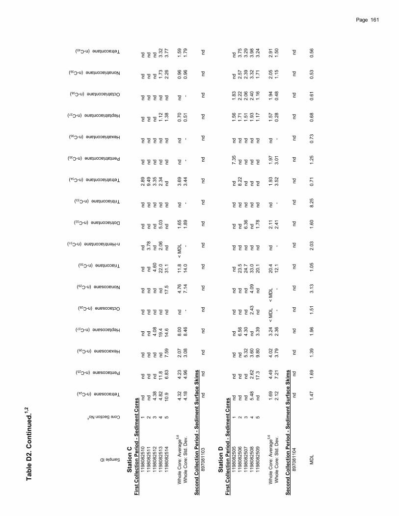
Tabl

e D

2. C

ontin

ued.

1,2

Sample ID

Core Section No4

Tetracosane (n-C24)

Pentacosane (n-C25)

Hexacosane (n-C26)

Heptacosane (n-C27)

Octacosane (n-C28)

Nonacosane (n-C29)

Triacontane (n-C30)

n-Hentriacontane (n-C31)

Dotriacontane (n-C32)

Tritriacontane (n-C33)

Tetratriacontane (n-C34)

Pentatriacontane (n-C35)

Hexatriacontane (n-C36)

Heptatriacontane (n-C37)

Octatriacontane (n-C38)

Nonatriacontane (n-C39)

Tetracontane (n-C40)

Stat

ion

CFi

rst C

olle

ctio

n Pe

riod

- Sed

imen

t Cor

es11

9808

2510

1

nd

nd

nd

nd

nd

nd

nd

nd

nd

nd

2.

89

nd

nd

nd

nd

nd

nd

11

9808

2511

2

nd

nd

nd

nd

nd

nd

nd

3.

78

nd

nd

9.

49

nd

nd

nd

nd

nd

nd

11

9808

2512

3

4.

38

nd

nd

4.

08

nd

nd

4.

60

nd

nd

nd

3.

35

nd

nd

nd

nd

nd

nd

11

9808

2513

4

4.

82

11.

8

nd

19.

4

nd

nd

22.

0

2.

06

5.

03

nd

2.

34

nd

nd

1.

12

nd

1.

73

3.

3211

9808

2514

5

10.

9

6.

83

7.

59

14.

6

nd

17.

5

31.

1

nd

nd

nd

nd

nd

nd

1.

38

nd

2.

26

3.

77

Who

le C

ore:

Ave

rage

5,6

4.32

4.23

2.07

8.00

n

d

4.76

1

1.8

< M

DL

1.

65

nd

3.

69

nd

nd

0.

70

nd

0.

96

1.

59W

hole

Cor

e: S

td. D

ev.

4.18

4.96

3.08

8.46

-

7.14

1

4.0

-

1.89

-

3.44

-

-

0.51

-

0.96

1.79

Seco

nd C

olle

ctio

n Pe

riod

- Sed

imen

t Sur

face

Ski

ms

8970

8110

3

n

d

n

d

n

d

n

d

n

d

n

d

n

d

n

d

n

d

n

d

n

d

n

d

n

d

n

d

n

d

n

d

n

d

Stat

ion

DFi

rst C

olle

ctio

n Pe

riod

- Sed

imen

t Cor

es11

9808

2505

1

nd

nd

nd

nd

nd

nd

nd

nd

nd

nd

nd

7.

35

nd

1.

56

1.

83

nd

nd

11

9808

2506

2

nd

nd

nd

6.

56

nd

nd

23.

5

nd

nd

nd

8.

22

nd

nd

1.

71

2.

22

2.

57

3.

7511

9808

2507

3

nd

nd

5.

32

4.

30

nd

nd

24.

7

nd

6.

36

nd

nd

nd

nd

1.

51

2.

06

2.

39

3.

2911

9808

2508

4

5.

48

2.

62

3.

60

nd

2.

43

4.

09

33.

0

nd

nd

nd

nd

nd

nd

1.

93

2.

40

3.

32

3.

9811

9808

2509

5

nd

17.

3

9.

80

3.

39

nd

nd

20.

1

nd

1.

78

nd

nd

nd

nd

1.

17

1.

16

1.

71

3.

24

Who

le C

ore:

Ave

rage

5,6

1.69

4.49

4.02

3.24

< M

DL

<

MD

L

2

0.4

n

d

2.11

n

d

1.93

1.97

n

d

1.57

1.94

2.05

2.91

Who

le C

ore:

Std

. Dev

.

2.

12

7.

21

3.

79

2.

36

-

-

12.

1

-

2.

41

-

3.

52

3.

01

-

0.

28

0.

48

1.

15

1.

50

Seco

nd C

olle

ctio

n Pe

riod

- Sed

imen

t Sur

face

Ski

ms

8970

8110

4

n

d

n

d

n

d

n

d

n

d

n

d

n

d

n

d

n

d

n

d

n

d

n

d

n

d

n

d

n

d

n

d

n

d

MD

L

1.

47

1.

69

1.

39

1.

96

1.

51

3.

13

1.

05

2.

03

1.

60

8.

25

0.

71

1.

25

0.

73

0.

68

0.

61

0.

53

0.

56

161Page

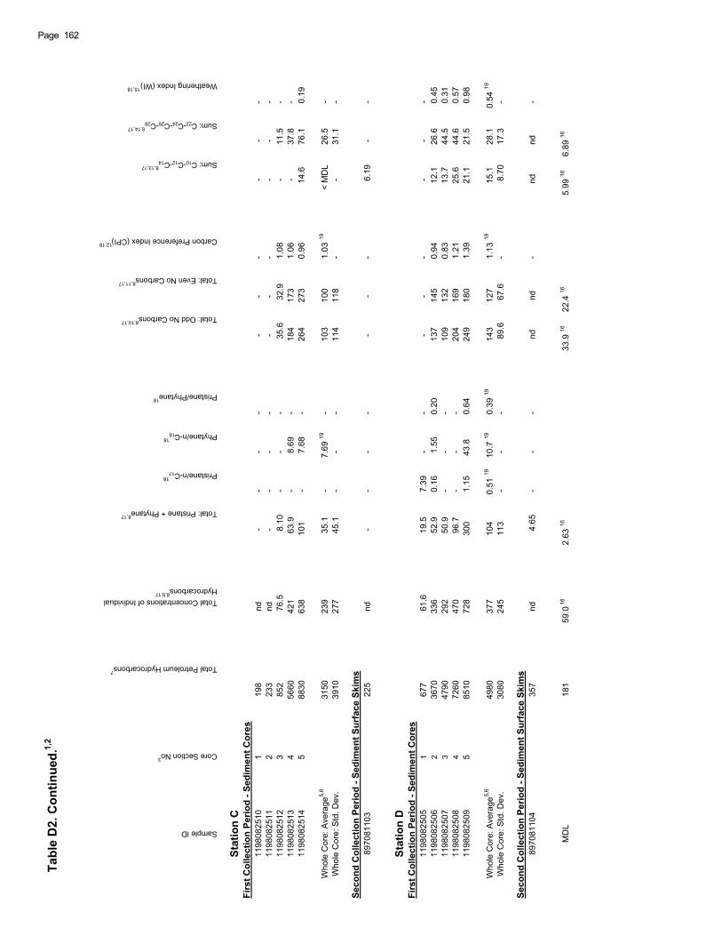
Tabl

e D

2. C

ontin

ued.

1,2

Sample ID

Core Section No3

Total Petroleum Hydrocarbons7

Total Concentrations of Individual Hydrocarbons

8,9,17

Total: Pristane + Phytane8,17

Pristane/n-C1718

Phytane/n-C1818

Pristane/Phytane18

Total: Odd No Carbons8,10,17

Total: Even No Carbons8,11,17

Carbon Preference Index (CPI)12,18

Sum: C10-C12-C148,13,17

Sum: C22-C24-C26-C288,14,17

Weathering Index (WI)15,18

Stat

ion

CFi

rst C

olle

ctio

n Pe

riod

- Sed

imen

t Cor

es11

9808

2510

1

198

nd

-

-

-

-

-

-

-

-

-

-

1198

0825

112

2

33

n

d

-

-

-

-

-

-

-

-

-

-11

9808

2512

3

852

76.

5

8.

10

-

-

-

35.

6

32.

9

1.

08

-

11.

5

-

1198

0825

134

56

60

4

21

6

3.9

-

8.69

-

1

84

1

73

1.06

-

3

7.8

-11

9808

2514

5

8830

638

101

-

7.

68

-

264

273

0.

96

14.

6

76.

1

0.

19

Who

le C

ore:

Ave

rage

5,6

31

50

2

39

3

5.1

-

7

.69

19

-

103

100

1.

03 19

< M

DL

26.

5

-

W

hole

Cor

e: S

td. D

ev.

39

10

2

77

4

5.1

-

-

-

1

14

1

18

-

-

3

1.1

-

Seco

nd C

olle

ctio

n Pe

riod

- Sed

imen

t Sur

face

Ski

ms

8970

8110

3

225

nd

-

-

-

-

-

-

-

6.

19

-

-

Stat

ion

DFi

rst C

olle

ctio

n Pe

riod

- Sed

imen

t Cor

es11

9808

2505

1

677

61.

6

19.

5

7.

39

-

-

-

-

-

-

-

-

11

9808

2506

2

3670

336

52.

9

0.

16

1.

55

0.

20

137

145

0.

94

12.

1

26.

6

0.

4511

9808

2507

3

4790

292

50.

9

-

-

-

109

132

0.

83

13.

7

44.

5

0.

3111

9808

2508

4

7260

470

96.

7

-

-

-

204

169

1.

21

25.

6

44.

6

0.

5711

9808

2509

5

8510

728

300

1.

15

43.

8

0.

64

249

180

1.

39

21.

1

21.

5

0.

98

Who

le C

ore:

Ave

rage

5,6

49

80

3

77

1

04

0

.51

19

10.

7 19

0.39

19

143

127

1.

13 19

1

5.1

2

8.1

0

.54

19

Who

le C

ore:

Std

. Dev

.

3080

245

113

-

-

-

89.

6

67.

6

-

8.

70

17.

3

-

Se

cond

Col

lect

ion

Perio

d - S

edim

ent S

urfa

ce S

kim

s89

7081

104

3

57

n

d

4.65

-

-

-

n

d

n

d

-

n

d

n

d

-

MD

L

181

59

.0 1

62.

6316

33.9

1622

.416

5.99

166.

8916

Page 162

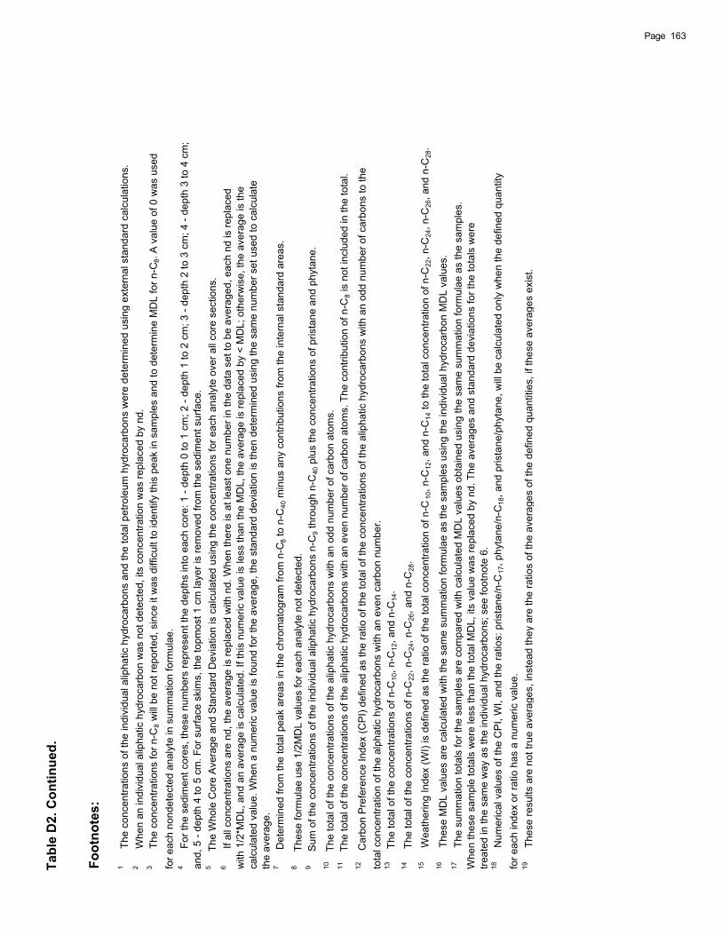
Tabl

e D

2. C

ontin

ued.

Foot

note

s:

1

The

conc

entra

tions

of t

he in

divi

dual

alip

hatic

hyd

roca

rbon

s an

d th

e to

tal p

etro

leum

hyd

roca

rbon

s w

ere

dete

rmin

ed u

sing

ext

erna

l sta

ndar

d ca

lcul

atio

ns.

2

Whe

n an

indi

vidu

al a

lipha

tic h

ydro

carb

on w

as n

ot d

etec

ted,

its

conc

entra

tion

was

repl

aced

by

nd.

3

The

conc

entra

tions

for n

-C8 w

ill b

e no

t rep

orte

d, s

ince

it w

as d

iffic

ult t

o id

entif

y th

is p

eak

in s

ampl

es a

nd to

det

erm

ine

MD

L fo

r n-C

8. A

val

ue o

f 0 w

as u

sed

for e

ach

nond

etec

ted

anal

yte

in s

umm

atio

n fo

rmul

ae.

4

For t

he s

edim

ent c

ores

, the

se n

umbe

rs re

pres

ent t

he d

epth

s in

to e

ach

core

: 1 -

dept

h 0

to 1

cm

; 2 -

dept

h 1

to 2

cm

; 3 -

dept

h 2

to 3

cm

; 4 -

dept

h 3

to 4

cm

;an

d, 5

- de

pth

4 to

5 c

m. F

or s

urfa

ce s

kim

s, th

e to

pmos

t 1 c

m la

yer i

s re

mov

ed fr

om th

e se

dim

ent s

urfa

ce.

5 T

he W

hole

Cor

e A

vera

ge a

nd S

tand

ard

Dev

iatio

n is

cal

cula

ted

usin

g th

e co

ncen

tratio

ns fo

r eac

h an

alyt

e ov

er a

ll co

re s

ectio

ns.

6

If al

l con

cent

ratio

ns a

re n

d, th

e av

erag

e is

repl

aced

with

nd.

Whe

n th

ere

is a

t lea

st o

ne n

umbe

r in

the

data

set

to b

e av

erag

ed, e

ach

nd is

repl

aced

w

ith 1

/2*M

DL,

and

an

aver

age

is c

alcu

late

d. If

this

num

eric

val

ue is

less

than

the

MD

L, th

e av

erag

e is

repl

aced

by

< M

DL;

oth

erw

ise,

the

aver

age

is th

eca

lcul

ated

val

ue. W

hen

a nu

mer

ic v

alue

is fo

und

for t

he a

vera

ge, t

he s

tand

ard

devi

atio

n is

then

det

erm

ined

usi

ng th

e sa

me

num

ber s

et u

sed

to c

alcu

late

the

aver

age.

7

Det

erm

ined

from

the

tota

l pea

k ar

eas

in th

e ch

rom

atog

ram

from

n-C

8 to

n-C

40 m

inus

any

con

tribu

tions

from

the

inte

rnal

sta

ndar

d ar

eas.

8 T

hese

form

ulae

use

1/2

MD

L va

lues

for e

ach

anal

yte

not d

etec

ted.

9 S

um o

f the

con

cent

ratio

ns o

f the

indi

vidu

al a

lipha

tic h

ydro

carb

ons

n-C

9 thr

ough

n-C

40 p

lus

the

conc

entra

tions

of p

rista

ne a

nd p

hyta

ne.

10 T

he to

tal o

f the

con

cent

ratio

ns o

f the

alip

hatic

hyd

roca

rbon

s w

ith a

n od

d nu

mbe

r of c

arbo

n at

oms.

11 T

he to

tal o

f the

con

cent

ratio

ns o

f the

alip

hatic

hyd

roca

rbon

s w

ith a

n ev

en n

umbe

r of c

arbo

n at

oms.

The

con

tribu

tion

of n

-C8 i

s no

t inc

lude

d in

the

tota

l.12

C

arbo

n P

refe

renc

e In

dex

(CP

I) de

fined

as

the

ratio

of t

he to

tal o

f the

con

cent

ratio

ns o

f the

alip

hatic

hyd

roca

rbon

s w

ith a

n od

d nu

mbe

r of c

arbo

ns to

the

tota

l con

cent

ratio

n of

the

alph

atic

hyd

roca

rbon

s w

ith a

n ev

en c

arbo

n nu

mbe

r.13

The

tota

l of t

he c

once

ntra

tions

of n

-C10

, n-C

12, a

nd n

-C14

.14

The

tota

l of t

he c

once

ntra

tions

of n

-C22

, n-C

24, n

-C26

, and

n-C

28.

15

Wea

ther

ing

Inde

x (W

I) is

def

ined

as

the

ratio

of t

he to

tal c

once

ntra

tion

of n

-C10

, n-C

12, a

nd n

-C14

to th

e to

tal c

once

ntra

tion

of n

-C22

, n-C

24, n

-C26

, and

n-C

28.

16

The

se M

DL

valu

es a

re c

alcu

late

d w

ith th

e sa

me

sum

mat

ion

form

ulae

as

the

sam

ples

usi

ng th

e in

divi

dual

hyd

roca

rbon

MD

L va

lues

.17

T

he s

umm

atio

n to

tals

for t

he s

ampl

es a

re c

ompa

red

with

cal

cula

ted

MD

L va

lues

obt

aine

d us

ing

the

sam

e su

mm

atio

n fo

rmul

ae a

s th

e sa

mpl

es.

Whe

n th

ese

sam

ple

tota

ls w

ere

less

than

the

tota

l MD

L, it

s va

lue

was

repl

aced

by

nd. T

he a

vera

ges

and

stan

dard

dev

iatio

ns fo

r the

tota

ls w

ere

treat

ed in

the

sam

e w

ay a

s th

e in

divi

dual

hyd

roca

rbon

s; s

ee fo

otno

te 6

.18

N

umer

ical

val

ues

of th

e C

PI,

WI,

and

the

ratio

s: p

rista

ne/n

-C17

, phy

tane

/n-C

18, a

nd p

rista

ne/p

hyta

ne, w

ill b

e ca

lcul

ated

onl

y w

hen

the

defin

ed q

uant

ityfo

r eac

h in

dex

or ra

tio h

as a

num

eric

val

ue.

19

The

se re

sults

are

not

true

ave

rage

s, in

stea

d th

ey a

re th

e ra

tios

of th

e av

erag

es o

f the

def

ined

qua

ntiti

es, i

f the

se a

vera

ges

exis

t.

163Page

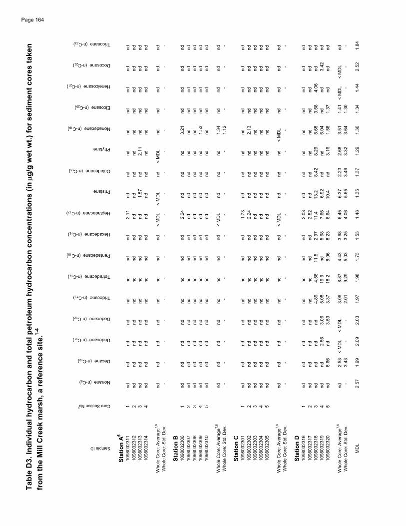
Tabl

e D

3. In

divi

dual

hyd

roca

rbon

and

tota

l pet

role

um h

ydro

carb

on c

once

ntra

tions

(in

g/g

wet

wt.)

for s

edim

ent c

ores

take

n fr

om th

e M

ill C

reek

mar

sh, a

refe

renc

e si

te.1-

4

Sample ID

Core Section No5

Nonane (n-C9)

Decane (n-C10)

Undecane (n-C11)

Dodecane (n-C12)

Tridecane (n-C13)

Tetradecane (n-C14)

Pentadecane (n-C15)

Hexadecane (n-C16)

Heptadecane (n-C17)

Pristane

Octadecane (n-C18)

Phytane

Nonadecane (n-C19)

Eicosane (n-C20)

Heneicosane (n-C21)

Docosane (n-C22)

Tricosane (n-C23)

Stat

ion

A6

1098

0323

111

n

d

n

d

n

d

n

d

n

d

n

d

n

d

n

d

2.11

n

d

n

d

n

d

n

d

n

d

n

d

n

d

n

d

1098

0323

122

n

d

n

d

n

d

n

d

n

d

n

d

n

d

n

d

n

d

n

d

n

d

n

d

n

d

n

d

n

d

n

d

n

d

1098

0323

133

n

d

n

d

n

d

n

d

n

d

n

d

n

d

n

d

n

d

1.57

n

d

2.11

n

d

n

d

n

d

n

d

n

d

1098

0323

144

n

d

n

d

n

d

n

d

n

d

n

d

n

d

n

d

n

d

n

d

n

d

n

d

n

d

n

d

n

d

n

d

n

d

Who

le C

ore:

Ave

rage

7,8

n

d

n

d

n

d

n

d

n

d

n

d

n

d

n

d

< M

DL

<

MD

L

n

d

< M

DL

nd

nd

nd

nd

nd

W

hole

Cor

e: S

td. D

ev.

-

-

-

-

-

-

-

-

-

-

-

-

-

-

-

-

-

Stat

ion

B10

9803

2306

1

nd

nd

nd

nd

nd

nd

nd

nd

2.

24

nd

nd

nd

3.

21

nd

nd

nd

nd

10

9803

2307

2

nd

nd

nd

nd

nd

nd

nd

nd

nd

nd

nd

nd

nd

nd

nd

nd

nd

10

9803

2308

3

nd

nd

nd

nd

nd

nd

nd

nd

nd

nd

nd

nd

nd

nd

nd

nd

nd

10

9803

2309

4

nd

nd

nd

nd

nd

nd

nd

nd

nd

nd

nd

nd

1.

53

nd

nd

nd

nd

10

9803

2310

5

nd

nd

nd

nd

nd

nd

nd

nd

nd

nd

nd

nd

nd

nd

nd

nd

nd

Who

le C

ore:

Ave

rage

7,8

n

d

n

d

n

d

n

d

n

d

n

d

n

d

n

d

< M

DL

nd

nd

nd

1.

34

nd

nd

nd

nd

W

hole

Cor

e: S

td. D

ev.

-

-

-

-

-

-

-

-

-

-

-

-

1.12

-

-

-

-

Stat

ion

C10

9803

2301

1

nd

nd

nd

nd

nd

nd

nd

nd

1.

73

nd

nd

nd

nd

nd

nd

nd

nd

10

9803

2302

2

nd

nd

nd

nd

nd

nd

nd

nd

2.

24

nd

nd

nd

2.

13

nd

nd

nd

nd

10

9803

2303

3

nd

nd

nd

nd

nd

nd

nd

nd

nd

nd

nd

nd

nd

nd

nd

nd

nd

10

9803

2304

4

nd

nd

nd

nd

nd

nd

nd

nd

nd

nd

nd

nd

nd

nd

nd

nd

nd

10

9803

2305

5

nd

nd

nd

nd

nd

nd

nd

nd

nd

nd

nd

nd

nd

nd

nd

nd

nd

Who

le C

ore:

Ave

rage

7,8

n

d

n

d

n

d

n

d

n

d

n

d

n

d

n

d

< M

DL

nd

nd

nd

<

MD

L

n

d

n

d

n

d

n

d

Who

le C

ore:

Std

. Dev

.

-

-

-

-

-

-

-

-

-

-

-

-

-

-

-

-

-

Stat

ion

D10

9803

2316

1

nd

nd

nd

nd

nd

nd

nd

nd

2.

03

nd

nd

nd

nd

nd

nd

nd

nd

10

9803

2317

2

nd

nd

nd

nd

nd

nd

nd

nd

2.

52

nd

nd

nd

nd

nd

nd

nd

nd

10

9803

2318

3

nd

nd

nd

nd

4.

89

4.

58

11.

5

2.

97

11.

4

13.

2

8.

42

8.

29

8.

65

3.

68

4.

06

nd

nd

10

9803

2319

4

nd

nd

2.

56

3.

06

5.

08

19.

6

nd

5.

68

7.

66

6.

92

nd

nd

6.

04

nd

nd

3.

42

nd

10

9803

2320

5

nd

8.

66

nd

3.

53

3.

37

18.

2

8.

06

8.

23

8.

64

10.

4

nd

3.

16

1.

58

1.

37

nd

nd

nd

Who

le C

ore:

Ave

rage

7,8

n

d

2.53

< M

DL

<

MD

L

3.06

8.87

4.43

3.68

6.45

6.37

2.23

2.68

3.51

1.41

< M

DL

<

MD

L

n

d

Who

le C

ore:

Std

. Dev

.

-

3.

43

-

-

2.

01

9.

29

5.

03

3.

25

4.

06

5.

65

3.

46

3.

32

3.

64

1.

30

-

-

-

MD

L

2.

57

1.

99

2.

09

2.

03

1.

97

1.

98

1.

73

1.

53

1.

48

1.

35

1.

37

1.

29

1.

30

1.

34

1.

44

2.

52

1.

84

Page 164

Tabl

e D

3. C

ontin

ued.

1-3

Sample ID

Core Section No5

Tetracosane (n-C24)

Pentacosane (n-C25)

Hexacosane (n-C26)

Heptacosane (n-C27)

Octacosane (n-C28)

Nonacosane (n-C29)

Triacontane (n-C30)

n-Hentriacontane (n-C31)

Dotriacontane (n-C32)

Tritriacontane (n-C33)

Tetratriacontane (n-C34)

Pentatriacontane (n-C35)

Hexatriacontane (n-C36)

Heptatriacontane (n-C37)

Octatriacontane (n-C38)

Nonatriacontane (n-C39)

Tetracontane (n-C40)

Stat

ion

A6

1098

0323

111

n

d

n

d

n

d

n

d

n

d

3.66

n

d

7.61

n

d

1

7.9

n

d

n

d

n

d

n

d

n

d

n

d

n

d

1098

0323

122

n

d

n

d

n

d

n

d

n

d

3.90

n

d

7.02

n

d

n

d

n

d

n

d

n

d

n

d

n

d

n

d

n

d

1098

0323

133

n

d

n

d

n

d

n

d

n

d

n

d

n

d

5.26

n

d

2

0.2

n

d

n

d

1.52

n

d

n

d

n

d

n

d

1098

0323

144

n

d

n

d

n

d

n

d

n

d

3.56

n

d

6.29

n

d

n

d

n

d

n

d

1.91

n

d

n

d

n

d

n

d

Who

le C

ore:

Ave

rage

7,8

n

d

n

d

n

d

n

d

n

d

3.17

n

d

6.54

n

d

1

1.6

n

d

n

d

1.04

n

d

n

d

n

d

n

d

Who

le C

ore:

Std

. Dev

.

-

-

-

-

-

1.

08

-

1.

01

-

8.

67

-

-

0.

80

-

-

-

-

Stat

ion

B10

9803

2306

1

nd

nd

nd

nd

nd

3.

47

nd

8.

38

nd

17.

1

nd

nd

nd

nd

nd

nd

nd

10

9803

2307

2

nd

nd

nd

nd

nd

nd

nd

nd

nd

nd

nd

nd

nd

nd

nd

nd

nd

10

9803

2308

3

nd

nd

nd

nd

nd

3.

56

nd

7.

45

nd

12.

7

nd

nd

0.

91

nd

nd

nd

nd

10

9803

2309

4

nd

nd

nd

nd

nd

nd

nd

5.

68

nd

32.

0

nd

nd

1.

92

nd

nd

nd

nd

10

9803

2310

5

nd

nd

nd

nd

nd

nd

nd

5.

73

nd

42.

4

nd

nd

1.

42

nd

nd

nd

nd

Who

le C

ore:

Ave

rage

7,8

n

d

n

d

n

d

n

d

n

d

< M

DL

nd

5.

65

nd

21.

7

nd

nd

1.

00

nd

nd

nd

nd

W

hole

Cor

e: S

td. D

ev.

-

-

-

-

-

-

-

2.84

-

1

5.4

-

-

0.68

-

-

-

-

Stat

ion

C10

9803

2301

1

nd

nd

nd

nd

nd

nd

nd

8.

18

nd

18.

2

nd

nd

nd

nd

nd

nd

nd

10

9803

2302

2

nd

nd

nd

nd

nd

3.

61

nd

8.

02

1.

89

17.

6

nd

nd

nd

nd

nd

nd

nd

10

9803

2303

3

nd

nd

nd

nd

nd

4.

85

nd

8.

03

2.

21

nd

nd

nd

0.

90

nd

nd

nd

nd

10

9803

2304

4

nd

nd

nd

nd

nd

5.

27

nd

7.

23

2.

31

40.

7

nd

nd

0.

94

nd

nd

nd

nd

10

9803

2305

5

nd

nd

nd

nd

nd

4.

18

nd

7.

66

1.

95

nd

nd

nd

1.

07

nd

nd

nd

nd

Who

le C

ore:

Ave

rage

7,8

n

d

n

d

n

d

n

d

n

d

3.90

n

d

7.82

1.83

1

7.0

n

d

n

d

< M

DL

nd

nd

nd

nd

W

hole

Cor

e: S

td. D

ev.

-

-

-

-

-

1.45

-

0.38

0.60

1

5.0

-

-

-

-

-

-

-

Stat

ion

D10

9803

2316

1

nd

nd

nd

nd

nd

3.

29

nd

8.

66

2.

51

10.

3

nd

nd

nd

nd

nd

nd

nd

10

9803

2317

2

nd

nd

nd

nd

1.

63

3.

54

1.

65

5.

42

2.

02

nd

0.

74

nd

nd

nd

nd

nd

nd

10

9803

2318

3

nd

nd

1.

62

nd

3.

04

4.

42

3.

75

3.

05

nd

nd

nd

nd

nd

nd

nd

nd

nd

10

9803

2319

4

nd

nd

1.

89

2.

03

1.

74

3.

98

2.

77

2.

57

nd

nd

0.

74

nd

nd

nd

nd

nd

nd

10

9803

2320

5

nd

2.

13

nd

nd

3.

43

3.

81

nd

3.

01

nd

nd

nd

nd

nd

nd

nd

nd

nd

Who

le C

ore:

Ave

rage

7,8

n

d

<

MD

L

< M

DL

<

MD

L

2.12

3.81

1.85

4.54

< M

DL

<

MD

L

< M

DL

nd

nd

nd

nd

nd

nd

W

hole

Cor

e: S

td. D

ev.

-

-

-

-

1.10

0.43

1.42

2.56

-

-

-

-

-

-

-

-

-

MD

L

1.

47

1.

69

1.

39

1.

96

1.

51

3.

13

1.

05

2.

03

1.

60

8.

25

0.

71

1.

25

0.

73

0.

68

0.

61

0.

53

0.

56

165Page

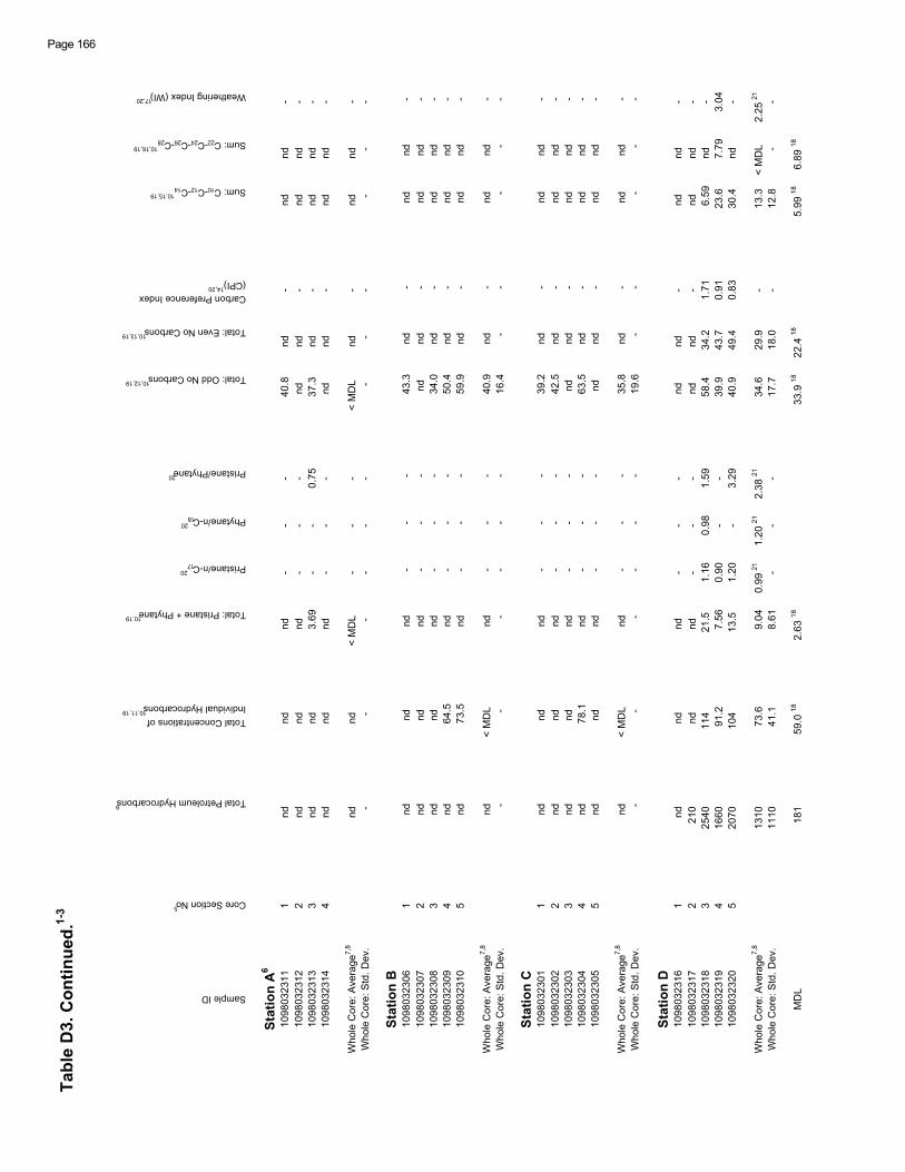
Tabl

e D

3. C

ontin

ued.

1-3

Sample ID

Core Section No5

Total Petroleum Hydrocarbons9

Total Concentrations of Individual Hydrocarbons

10,11,19

Total: Pristane + Phytane10,19

Pristane/n-C1720

Phytane/n-C1820

Pristane/Phytane20

Total: Odd No Carbons10,12,19

Total: Even No Carbons10,13,19

Carbon Preference Index (CPI)

14,20

Sum: C10-C12-C1410,15,19

Sum: C22-C24-C26-C2810,16,19

Weathering Index (WI)17,20

Stat

ion

A6

1098

0323

111

n

d

n

d

n

d

-

-

-

4

0.8

n

d

-

n

d

n

d

-10

9803

2312

2

nd

nd

nd

-

-

-

nd

nd

-

nd

nd

-

1098

0323

133

n

d

n

d

3.69

-

-

0.75

3

7.3

n

d

-

n

d

n

d

-10

9803

2314

4

nd

nd

nd

-

-

-

nd

nd

-

nd

nd

-

Who

le C

ore:

Ave

rage

7,8

n

d

n

d

< M

DL

-

-

-

<

MD

L

n

d

-

n

d

n

d

-

Who

le C

ore:

Std

. Dev

.

-

-

-

-

-

-

-

-

-

-

-

-

Stat

ion

B10

9803

2306

1

nd

nd

nd

-

-

-

43

.3

nd

-

nd

nd

-

1098

0323

072

nd

nd

nd

-

-

-

nd

nd

-

nd

nd

-10

9803

2308

3

nd

nd

nd

-

-

-

34

.0

nd

-

nd

nd

-

1098

0323

094

nd

64.5

nd

-

-

-

50.4

nd

-

nd

nd

-10

9803

2310

5

nd

73

.5

nd

-

-

-

59

.9

nd

-

nd

nd

-

Who

le C

ore:

Ave

rage

7,8

nd

<

MD

L

nd

-

-

-

40.9

nd

-

nd

nd

-

Who

le C

ore:

Std

. Dev

.

-

-

-

-

-

-

16

.4

-

-

-

-

-

Stat

ion

C10

9803

2301

1

nd

nd

nd

-

-

-

39

.2

nd

-

nd

nd

-

1098

0323

022

nd

nd

nd

-

-

-

42.5

nd

-

nd

nd

-10

9803

2303

3

nd

nd

nd

-

-

-

nd

nd

-

nd

nd

-

1098

0323

044

nd

78.1

nd

-

-

-

63.5

nd

-

nd

nd

-10

9803

2305

5

nd

nd

nd

-

-

-

nd

nd

-

nd

nd

-

Who

le C

ore:

Ave

rage

7,8

nd

<

MD

L

nd

-

-

-

35.8

nd

-

nd

nd

-

Who

le C

ore:

Std

. Dev

.

-

-

-

-

-

-

19

.6

-

-

-

-

-

Stat

ion

D10

9803

2316

1

nd

nd

nd

-

-

-

nd

nd

-

nd

nd

-

1098

0323

172

2

10

n

d

n

d

-

-

-

n

d

n

d

-

n

d

n

d

-10

9803

2318

3

2540

114

21.

5

1.

16

0.

98

1.

59

58.

4

34.

2

1.

71

6.

59

nd

-

1098

0323

194

16

60

9

1.2

7.56

0.90

-

-

3

9.9

4

3.7

0.91

2

3.6

7.79

3.04

1098

0323

205

20

70

1

04

1

3.5

1.20

-

3.29

4

0.9

4

9.4

0.83

3

0.4

n

d

-

Who

le C

ore:

Ave

rage

7,8

13

10

7

3.6

9.04

0

.99

21

1.2

0 21

2

.38

21

34.

6

29.

9

-

13.

3 <

MD

L

2

.25

21

Who

le C

ore:

Std

. Dev

.

1110

41.

1

8.

61

-

-

-

17.

7

18.

0

-

12.

8

-

-

MD

L

181

59

.0 18

2.63

1833

.918

22.4

185.

9918

6.89

18

Page 166

Tabl

e D

3. C

ontin

ued.

Foot

note

s:

1

No

surfa

ce s

kim

sam

ples

wer

e an

alyz

ed fo

r Mill

Cre

ek M

arsh

.2

Th

e co

ncen

tratio

ns o

f the

indi

vidu

al a

lipha

tic h

ydro

carb

ons

and

the

tota

l pet

role

um h

ydro

carb

ons

wer

e de

term

ined

usi

ng e

xter

nal s

tand

ard

calc

ulat

ions

.3

W

hen

an in

divi

dual

alip

hatic

hyd

roca

rbon

was

not

det

ecte

d, it

s co

ncen

tratio

n w

as re

plac

ed b

y nd

.4

Th

e co

ncen

tratio

ns fo

r n-C

8 will

be

not r

epor

ted,

sin

ce it

was

diff

icul

t to

iden

tify

this

pea

k in

sam

ples

and

to d

eter

min

e M

DL

for n

-C8.

A v

alue

of 0

was

use

dfo

r eac

h no

ndet

ecte

d an

alyt

e in

sum

mat

ion

form

ulae

.5

Fo

r the

sed

imen

t cor

es, t

hese

num

bers

repr

esen

t the

dep

ths

into

eac

h co

re: 1

- de

pth

0 to

1 c

m; 2

- de

pth

1 to

2 c

m; 3

- de

pth

2 to

3 c

m; 4

- de

pth

3 to

4 c

m;

and,

5 -

dept

h 4

to 5

cm

.6

Th

e ex

tract

for c

ore

sect

ion

5 fo

r Sta

tion

A w

as lo

st d

urin

g sa

mpl

e cl

eanu

p.7

Th

e W

hole

Cor

e A

vera

ge a

nd S

tand

ard

Dev

iatio

n is

cal

cula

ted

usin

g th

e co

ncen

tratio

ns fo

r eac

h an

alyt

e ov

er a

ll co

re s

ectio

ns.

8

If al

l con

cent

ratio

ns a

re n

d, th

e av

erag

e is

repl

aced

with

nd.

Whe

n th

ere

is a

t lea

st o

ne n

umbe

r in

the

data

set

to b

e av

erag

ed, e

ach

nd is

repl

aced

w

ith 1

/2*M

DL,

and

an

aver

age

is c

alcu

late

d. If

this

num

eric

val

ue is

less

than

the

MD

L, th

e av

erag

e is

repl

aced

by

< M

DL;

oth

erw

ise,

the

aver

age

is th

eca

lcul

ated

val

ue. W

hen

a nu

mer

ic v

alue

is fo

und

for t

he a

vera

ge, t

he s

tand

ard

devi

atio

n is

then

det

erm

ined

usi

ng th

e sa

me

num

ber s

et u

sed

to c

alcu

late

the

aver

age.

9

Det

erm

ined

from

the

tota

l pea

k ar

eas

in th

e ch

rom

atog

ram

from

n-C

8 to

n-C

40 m

inus

any

con

tribu

tions

from

the

inte

rnal

sta

ndar

d ar

eas.

10

The

se fo

rmul

ae u

se 1

/2M

DL

valu

es fo

r eac

h an

alyt

e no

t det

ecte

d.11

S

um o

f the

con

cent

ratio

ns o

f the

indi

vidu

al a

lipha

tic h

ydro

carb

ons

n-C

9 thr

ough

n-C

40 p

lus

the

conc

entra

tions

of p

rista

ne a

nd p

hyta

ne.

12 T

he to

tal o

f the

con

cent

ratio

ns o

f the

alip

hatic

hyd

roca

rbon

s w

ith a

n od

d nu

mbe

r of c

arbo

n at

oms.

13 T

he to

tal o

f the

con

cent

ratio

ns o

f the

alip

hatic

hyd

roca

rbon

s w

ith a

n ev

en n

umbe

r of c

arbo

n at

oms.

The

con

tribu

tion

of n

-C8 i

s no

t inc

lude

d in

the

tota

l.14

C

arbo

n P

refe

renc

e In

dex

(CP

I) de

fined

as

the

ratio

of t

he to

tal o

f the

con

cent

ratio

ns o

f the

alip

hatic

hyd

roca

rbon

s w

ith a

n od

d nu

mbe

r of c

arbo

ns to

the

tota

l con

cent

ratio

n of

the

alph

atic

hyd

roca

rbon

s w

ith a

n ev

en c

arbo

n nu

mbe

r.15

The

tota

l of t

he c

once

ntra

tions

of n

-C10

, n-C

12, a

nd n

-C14

.16

The

tota

l of t

he c

once

ntra

tions

of n

-C22

, n-C

24, n

-C26

, and

n-C

28.

17

Wea

ther

ing

Inde

x (W

I) is

def

ined

as

the

ratio

of t

he to

tal c

once

ntra

tion

of n

-C10

, n-C

12, a

nd n

-C14

to th

e to

tal c

once

ntra

tion

of n

-C22

, n-C

24, n

-C26

, and

n-C

28.

18

The

se M

DL

valu

es a

re c

alcu

late

d w

ith th

e sa

me

sum

mat

ion

form

ulae

as

the

sam

ples

usi

ng th

e in

divi

dual

hyd

roca

rbon

MD

L va

lues

.19

T

he s

umm

atio

n to

tals

for t

he s

ampl

es a

re c

ompa

red

with

cal

cula

ted

MD

L va

lues

obt

aine

d us

ing

the

sam

e su

mm

atio

n fo

rmul

ae a

s th

e sa

mpl

es.

Whe

n th

ese

sam

ple

tota

ls w

ere

less

than

the

tota

l MD

L, it

s va

lue

was

repl

aced

by

nd. T

he a

vera

ges

and

stan

dard

dev

iatio

ns fo

r the

tota

ls w

ere

treat

ed in

the

sam

e w

ay a

s th

e in

divi

dual

hyd

roca

rbon

s; s

ee fo

otno

te 8

.20

N

umer

ical

val

ues

of th

e C

PI,

WI,

and

the

ratio

s: p

rista

ne/n

-C17

, phy

tane

/n-C

18, a

nd p

rista

ne/p

hyta

ne, w

ill b

e ca

lcul

ated

onl

y w

hen

the

defin

ed q

uant

ityfo

r eac

h in

dex

or ra

tio h

as a

num

eric

val

ue.

21

The

se re

sults

are

not

true

ave

rage

s, in

stea

d th

ey a

re th

e ra

tios

of th

e av

erag

es o

f the

def

ined

qua

ntiti

es, i

f the

se a

vera

ges

exis

t.

167Page

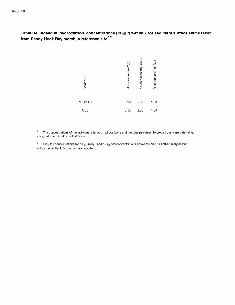
Table D4. Individual hydrocarbon concentrations (in g/g wet wt.) for sediment surface skims taken from Sandy Hook Bay marsh, a reference site.1,2

Sam

ple

ID

Non

acos

ane

(n-C

29)

n-H

entri

acon

tane

(n-

C31

)

Dot

riaco

ntan

e (n

-C32

)

897081116 6.19 5.09 1.68

MDL 3.13 2.03 1.60

1 The concentrations of the individual aliphatic hydrocarbons and the total petroleum hydrocarbons were determinedusing external standard calculations.

2 Only the concentrations for n-C29, n-C31, and n-C32 had concentrations above the MDL; all other analytes hadvalues below the MDL and are not reported.

Page 168

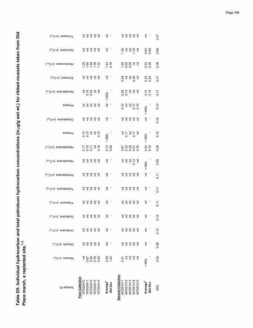
Tabl

e D

5. In

divi

dual

hyd

roca

rbon

and

tota

l pet

role

um h

ydro

carb

on c

once

ntra

tions

(in

g/g

wet

wt.)

for r

ibbe

d m

usse

ls ta

ken

from

Old

Pl

ace

mar

sh, a

repl

ante

d si

te.1-

3

Sample ID

Nonane (n-C9)

Decane (n-C10)

Undecane (n-C11)

Dodecane (n-C12)

Tridecane (n-C13)

Tetradecane (n-C14)

Pentadecane (n-C15)

Hexadecane (n-C16)

Heptadecane (n-C17)

Pristane

Octadecane (n-C18)

Phytane

Nonadecane (n-C19)

Eicosane (n-C20)

Heneicosane (n-C21)

Docosane (n-C22)

Tricosane (n-C23)

Firs

t Col

lect

ion

1970

2041

0nd

ndnd

ndnd

ndnd

nd0.

170.

12nd

ndnd

nd1.

25nd

nd19

7020

411

2.67

ndnd

ndnd

ndnd

nd0.

150.

12nd

nd0.

16nd

1.60

ndnd

1970

2041

20.

50nd

ndnd

ndnd

ndnd

0.11

ndnd

nd0.

22nd

1.59

ndnd

1970

2041

30.

76nd

ndnd

ndnd

ndnd

ndnd

ndnd

ndnd

1.36

ndnd

1970

2041

40.

43nd

ndnd

ndnd

ndnd

0.18

0.12

ndnd

ndnd

1.32

ndnd

Ave

rage

40.

90nd

ndnd

ndnd

ndnd

0.13

< M

DL

ndnd

< M

DL

nd1.

43nd

ndSt

d D

ev1.

02-

--

--

--

0.06

--

--

-0.

16-

-

Seco

nd C

olle

ctio

n49

7051

411

0.31

ndnd

ndnd

ndnd

nd0.

67nd

nd0.

100.

300.

541.

051.

35nd

4970

5141

2nd

ndnd

ndnd

ndnd

nd0.

320.

11nd

nd0.

13nd

0.65

ndnd

4970

5141

3nd

ndnd

ndnd

ndnd

nd0.

28nd

ndnd

ndnd

0.56

ndnd

4970

5141

4nd

ndnd

ndnd

ndnd

0.13

0.57

0.17

nd0.

17nd

0.36

nd1.

79nd

4970

5141

5nd

ndnd

ndnd

ndnd

nd0.

25nd

nd0.

10nd

ndnd

ndnd

Ave

rage

4<

MD

Lnd

ndnd

ndnd

nd<

MD

L0.

42<

MD

Lnd

< M

DL

0.12

0.24

0.53

0.83

ndSt

d D

ev-

--

--

--

-0.

19-

--

0.10

0.20

0.36

0.69

-

MD

L0.

240.

060.

120.

120.

110.

110.

110.

090.

080.

100.

100.

100.

110.

210.

380.

682.

47

Page 169

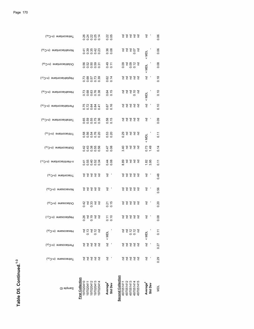
Tabl

e D

5. C

ontin

ued.

1-3

Sample ID

Tetracosane (n-C24)

Pentacosane (n-C25)

Hexacosane (n-C26)

Heptacosane (n-C27)

Octacosane (n-C28)

Nonacosane (n-C29)

Triacontane (n-C30)

n-Hentriacontane (n-C31)

Dotriacontane (n-C32)

Tritriacontane (n-C33)

Tetratriacontane (n-C34)

Pentatriacontane (n-C35)

Hexatriacontane (n-C36)

Heptatriacontane (n-C37)

Octatriacontane (n-C38)

Nonatriacontane (n-C39)

Tetracontane (n-C40)

Firs

t Col

lect

ion

1970

2041

0nd

ndnd

0.26

0.42

ndnd

0.41

0.42

0.58

0.65

0.75

0.73

0.73

0.56

0.41

0.26

1970

2041

1nd

nd0.

13nd

ndnd

nd0.

550.

430.

560.

590.

720.

680.

680.

520.

390.

2419

7020

412

ndnd

nd0.

190.

33nd

nd0.

400.

380.

540.

550.

640.

630.

570.

500.

350.

2219

7020

413

ndnd

0.12

ndnd

ndnd

0.52

0.55

0.76

0.75

0.84

0.76

0.73

0.59

0.42

0.25

1970

2041

4nd

ndnd

ndnd

ndnd

0.34

0.56

0.20

0.36

0.41

0.38

0.39

0.31

0.23

0.14

Ave

rage

4nd

nd<

MD

L0.

110.

21nd

nd0.

440.

470.

530.

580.

670.

640.

620.

490.

360.

22St

d D

ev-

--

0.10

0.15

--

0.08

0.08

0.20

0.15

0.16

0.15

0.14

0.11

0.08

0.05

Seco

nd C

olle

ctio

n49

7051

411

ndnd

ndnd

ndnd

nd8.

893.

400.

29nd

ndnd

nd0.

09nd

nd49

7051

412

ndnd

ndnd

ndnd

ndnd

ndnd

ndnd

ndnd

ndnd

nd49

7051

413

ndnd

0.12

ndnd

ndnd

ndnd

ndnd

ndnd

nd0.

09nd

nd49

7051

414

ndnd

0.12

ndnd

ndnd

ndnd

ndnd

nd0.

10nd

0.12

0.07

nd49

7051

415

ndnd

ndnd

ndnd

ndnd

ndnd

ndnd

ndnd

ndnd

nd

Ave

rage

4nd

nd<

MD

Lnd

ndnd

nd1.

820.

73<

MD

Lnd

nd<

MD

Lnd

< M

DL

< M

DL

ndSt

d D

ev-

--

--

--

3.95

1.49

--

--

--

--

MD

L0.

290.

270.

110.

080.

200.

560.

480.

110.

140.

110.

090.

100.

100.

180.

080.

060.

06

Page 170

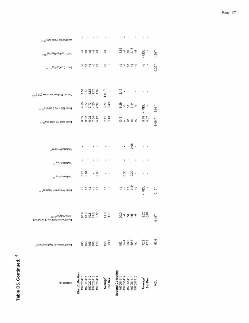
Tabl

e D

5. C

ontin

ued.

1-3

Sample ID

Total Petroleum Hydrocarbons5

Total Concentrations of Individual Hydrocarbons

6,7,15

Total: Pristane + Phytane6,15

Pristane/n-C1716

Phytane/n-C1816

Pristane/Phytane16

Total: Odd No Carbons6,8,15

Total: Even No Carbons6,9,15

Carbon Preference Index (CPI)10,16

Sum: C10-C12-C146,11,15

Sum: C22-C24-C26-C286,12,15

Weathering Index (WI)13,16

Firs

t Col

lect

ion

1970

2041

0

203

10.

9

nd

0.

73

-

-

6.

55

4.

16

1.

57

nd

nd

-

1970

2041

1

158

13.

3

nd

0.

84

-

-

9.

32

3.

77

2.

48

nd

nd

-

1970

2041

2

165

10.

8

nd

-

-

-

6.

92

3.

73

1.

86

nd

nd

-

1970

2041

3

106

11.

6

nd

-

-

-

7.

34

4.

20

1.

75

nd

nd

-

1970

2041

4

118

8.

55

nd

0.

63

-

-

5.

42

2.

97

1.

82

nd

nd

-

Ave

rage

4

150

11.

0

nd

-

-

-

7.

11

3.

77

1.8

9 17

n

d

n

d

-

Std

Dev

3

9.1

1.70

-

-

-

-

1.43

0.49

-

-

-

-

Seco

nd C

olle

ctio

n49

7051

411

1

52

2

0.0

n

d

-

-

-

1

3.5

6.29

2.15

n

d

1.66

- 49

7051

412

5

4.4

n

d

n

d

0.33

-

-

n

d

n

d

-

n

d

n

d

- 49

7051

413

5

8.6

n

d

n

d

-

-

-

n

d

n

d

-

n

d

n

d

- 49

7051

414

6

9.4

n

d

0.34

0.29

-

0.96

n

d

3.44

-

n

d

2.16

- 49

7051

415

n

d

n

d

n

d

-

-

-

n

d

n

d

-

n

d

n

d

-

Ave

rage

4

72.

2

8.

20 <

MD

L

-

-

-

5.18

< M

DL

-

nd

<

MD

L

-

Std

Dev

4

7.1

6.64

-

-

-

-

4.67

-

-

-

-

-

MD

L

53

.68.

1914

0.19

145.

0914

2.91

140.

2914

1.29

14

171Page

Tabl

e D

5. C

ontin

ued.

Foot

note

s:1

Th

e co

ncen

tratio

ns o

f the

indi

vidu

al a

lipha

tic h

ydro

carb

ons

and

the

tota

l pet

role

um h

ydro

carb

ons

wer

e de

term

ined

usi

ng e

xter

nal s

tand

ard

calc

ulat

ions

.2

W

hen

an in

divi

dual

alip

hatic

hyd

roca

rbon

was

not

det

ecte

d, it

s co

ncen

tratio

n w

as re

plac

ed b

y nd

.3

Th

e co

ncen

tratio

ns fo

r n-C

8 will

be

not r

epor

ted,

sin

ce it

was

diff

icul

t to

iden

tify

this

pea

k in

sam

ples

and

to d

eter

min

e M

DL

for n

-C8.

4

If al

l con

cent

ratio

ns a

re n

d, th

e av

erag

e is

repl

aced

with

nd.

Whe

n th

ere

is a

t lea

st o

ne n

umbe

r in

the

data

set

to b

e av

erag

ed, e

ach

nd is

repl

aced

w

ith 1

/2*M

DL,

and

an

aver

age

is c

alcu

late

d. If

this

num

eric

val

ue is

less

than

the

MD

L, th

e av

erag

e is

repl

aced

by

< M

DL;

oth

erw

ise,

the

aver

age

is th

eca

lcul

ated

val

ue. W

hen

a nu

mer

ic v

alue

is fo

und

for t

he a

vera

ge, t

he s

tand

ard

devi

atio

n is

then

det

erm

ined

usi

ng th

e sa

me

num

ber s

et u

sed

to c

alcu

late

the

aver

age.

5

D

eter

min

ed fr

om th

e to

tal p

eak

area

s in

the

chro

mat

ogra

m fr

om n

-C8 t

o n-

C40

min

us a

ny c

ontri

butio

ns fr

om th

e in

tern

al s

tand

ard

area

s.6

Th

ese

form

ulae

use

1/2

MD

L va

lues

for e

ach

anal

yte

not d

etec

ted.

7

Sum

of t

he c

once

ntra

tions

of t

he in

divi

dual

alip

hatic

hyd

roca

rbon

s n-

C9 t

hrou

gh n

-C40

plu

s th

e co

ncen

tratio

ns o

f pris

tane

and

phy

tane

.8

Th

e to

tal o

f the

con

cent

ratio

ns o

f the

alip

hatic

hyd

roca

rbon

s w

ith a

n od

d nu

mbe

r of c

arbo

n at

oms.

9

The

tota

l of t

he c

once

ntra

tions

of t

he a

lipha

tic h

ydro

carb

ons

with

an

even

num

ber o

f car

bon

atom

s. T

he c

ontri

butio

n of

n-C

8 is

not i

nclu

ded

in th

e to

tal.

10

Car

bon

Pre

fere

nce

Inde

x (C

PI)

defin

ed a

s th

e ra

tio o

f the

tota

l of t

he c

once

ntra

tions

of t

he a

lipha

tic h

ydro

carb

ons

with

an

odd

num

ber o

f car

bons

to th

eto

tal c

once

ntra

tion

of th

e al

phat

ic h

ydro

carb

ons

with

an

even

car

bon

num

ber.

11Th

e to

tal o

f the

con

cent

ratio

ns o

f n-C

10, n

-C12

, and

n-C

14.

12 T

he to

tal o

f the

con

cent

ratio

ns o

f n-C

22, n

-C24

, n-C

26, a

nd n

-C28

.13

W

eath

erin

g In

dex

(WI)

is d

efin

ed a

s th

e ra

tio o

f the

tota

l con

cent

ratio

n of

n-C

10, n

-C12

, and

n-C

14 to

the

tota

l con

cent

ratio

n of

n-C

22, n

-C24

, n-C

26, a

nd n

-C28

.14

T

hese

MD

L va

lues

are

cal

cula

ted

with

the

sam

e su

mm

atio

n fo

rmul

ae a

s th

e sa

mpl

es u

sing

the

indi

vidu

al h

ydro

carb

on M

DL

valu

es.

15

The

sum

mat

ion

tota

ls fo

r the

sam

ples

are

com

pare

d w

ith c

alcu

late

d M

DL

valu

es o

btai

ned

usin

g th

e sa

me

sum

mat

ion

form

ulae

as

the

sam

ples

.W

hen

thes

e sa

mpl

e to

tals

wer

e le

ss th

an th

e to

tal M

DL,

its

valu

e w

as re

plac

ed b

y nd

. The

ave

rage

s an

d st

anda

rd d

evia

tions

for t

he to

tals

wer

etre

ated

in th

e sa

me

way

as

the

indi

vidu

al h

ydro

carb

ons;

see

foot

note

4.

16

Num

eric

al v

alue

s of

the

CP

I, W

I, an

d th

e ra

tios:

pris

tane

/n-C

17, p

hyta

ne/n

-C18

, and

pris

tane

/phy

tane

, will

be

calc

ulat

ed o

nly

whe

n th

e de

fined

qua

ntity

for e

ach

inde

x or

ratio

has

a n

umer

ic v

alue

.17

T

hese

resu

lts a

re n

ot tr

ue a

vera

ges,

inst

ead

they

are

the

ratio

s of

the

aver

ages

of t

he d

efin

ed q

uant

ities

, if t

hese

ave

rage

s ex

ist.

Page 172

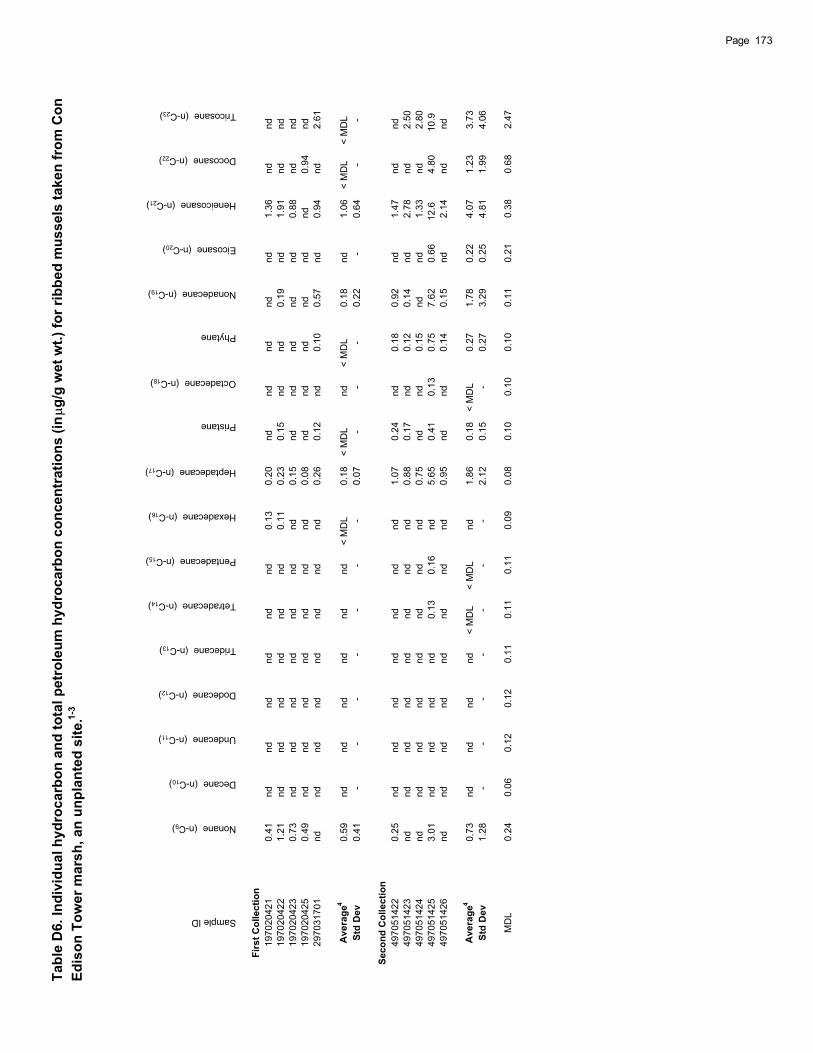
Tabl

e D

6. In

divi

dual

hyd

roca

rbon

and

tota

l pet

role

um h

ydro

carb

on c

once

ntra

tions

(in

g/g

wet

wt.)

for r

ibbe

d m

usse

ls ta

ken

from

Con

Ed

ison

Tow

er m

arsh

, an

unpl

ante

d si

te.1-

3

Sample ID

Nonane (n-C9)

Decane (n-C10)

Undecane (n-C11)

Dodecane (n-C12)

Tridecane (n-C13)

Tetradecane (n-C14)

Pentadecane (n-C15)

Hexadecane (n-C16)

Heptadecane (n-C17)

Pristane

Octadecane (n-C18)

Phytane

Nonadecane (n-C19)

Eicosane (n-C20)

Heneicosane (n-C21)

Docosane (n-C22)

Tricosane (n-C23)

Firs

t Col

lect

ion

1970

2042

1

0.

41

nd

nd

nd

nd

nd

nd

0.

13

0.

20

nd

nd

nd

nd

nd

1.

36

nd

nd

19

7020

422

1.21

n

d

n

d

n

d

n

d

n

d

n

d

0.11

0.23

0.15

n

d

n

d

0.19

n

d

1.91

n

d

n

d

1970

2042

3

0.

73

nd

nd

nd

nd

nd

nd

nd

0.

15

nd

nd

nd

nd

nd

0.

88

nd

nd

19

7020

425

0.49

n

d

n

d

n

d

n

d

n

d

n

d

n

d

0.08

n

d

n

d

n

d

n

d

n

d

n

d

0.94

n

d

2970

3170

1

nd

nd

nd

nd

nd

nd

nd

nd

0.

26

0.

12

nd

0.

10

0.

57

nd

0.

94

nd

2.

61

Ave

rage

4

0.

59

nd

nd

nd

nd

nd

nd

<

MD

L

0.18

< M

DL

nd

<

MD

L

0.18

n

d

1.06

< M

DL

<

MD

L

Std

Dev

0.41

-

-

-

-

-

-

-

0.07

-

-

-

0.22

-

0.64

-

-

Seco

nd C

olle

ctio

n49

7051

422

0.25

n

d

n

d

n

d

n

d

n

d

n

d

n

d

1.07

0.24

n

d

0.18

0.92

n

d

1.47

n

d

n

d

4970

5142

3

nd

nd

nd

nd

nd

nd

nd

nd

0.

88

0.

17

nd

0.

12

0.

14

nd

2.

78

nd

2.

5049

7051

424

n

d

n

d

n

d

n

d

n

d

n

d

n

d

n

d

0.75

n

d

n

d

0.15

n

d

n

d

1.33

n

d

2.80

4970

5142

5

3.

01

nd

nd

nd

nd

0.

13

0.

16

nd

5.

65

0.

41

0.

13

0.

75

7.

62

0.

66

12.

6

4.

80

10.

9 49

7051

426

n

d

n

d

n

d

n

d

n

d

n

d

n

d

n

d

0.95

n

d

n

d

0.14

0.15

n

d

2.14

n

d

n

d

Ave

rage

4

0.

73

nd

nd

nd

nd

<

MD

L

< M

DL

nd

1.

86

0.

18

< M

DL

0.

27

1.

78

0.

22

4.

07

1.

23

3.

73St

d D

ev

1.

28

-

-

-

-

-

-

-

2.

12

0.

15

-

0.

27

3.

29

0.

25

4.

81

1.

99

4.

06

MD

L0.

240.

060.

120.

120.

110.

110.

110.

090.

080.

100.

100.

100.

110.

210.

380.

682.

47

173Page

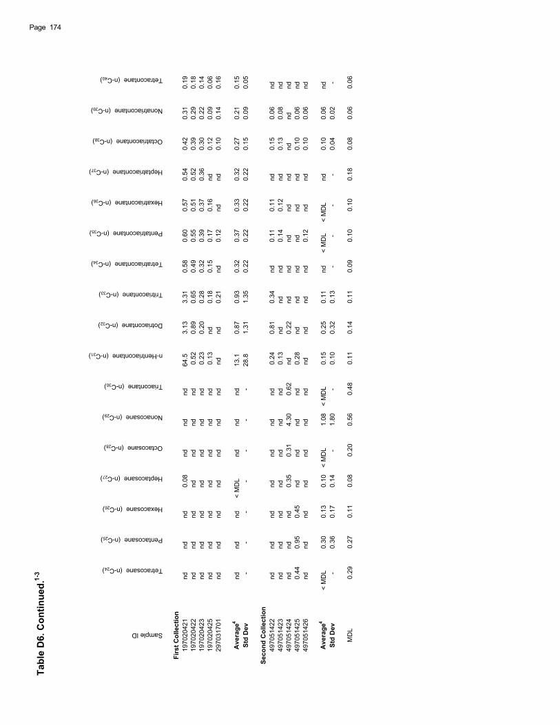
Tabl

e D

6. C

ontin

ued.

1-3

Sample ID

Tetracosane (n-C24)

Pentacosane (n-C25)

Hexacosane (n-C26)

Heptacosane (n-C27)

Octacosane (n-C28)

Nonacosane (n-C29)

Triacontane (n-C30)

n-Hentriacontane (n-C31)

Dotriacontane (n-C32)

Tritriacontane (n-C33)

Tetratriacontane (n-C34)

Pentatriacontane (n-C35)

Hexatriacontane (n-C36)

Heptatriacontane (n-C37)

Octatriacontane (n-C38)

Nonatriacontane (n-C39)

Tetracontane (n-C40)

Firs

t Col

lect

ion

1970

2042

1

nd

nd

nd

0.

08

nd

nd

nd

64.

5

3.

13

3.

31

0.

58

0.

60

0.

57

0.

54

0.

42

0.

31

0.

1919

7020

422

n

d

n

d

n

d

n

d

n

d

n

d

n

d

0.52

0.89

0.65

0.49

0.55

0.51

0.52

0.39

0.29

0.18

1970

2042

3

nd

nd

nd

nd

nd

nd

nd

0.

23

0.

20

0.

28

0.

32

0.

39

0.

37

0.

36

0.

30

0.

22

0.

1419

7020

425

n

d

n

d

n

d

n

d

n

d

n

d

n

d

0.13

n

d

0.18

0.15

0.17

0.16

n

d

0.12

0.09

0.06

2970

3170

1

nd

nd

nd

nd

nd

nd

nd

nd

nd

0.

21

nd

0.

12

nd

nd

0.

10

0.

14

0.

16

Ave

rage

4

nd

nd

nd

< M

DL

nd

nd

nd

13.

1

0.

87

0.

93

0.

32

0.

37

0.

33

0.

32

0.

27

0.

21

0.

15St

d D

ev

-

-

-

-

-

-

-

28.

8

1.

31

1.

35

0.

22

0.

22

0.

22

0.

22

0.

15

0.

09

0.

05

Seco

nd C

olle

ctio

n49

7051

422

n

d

n

d

n

d

n

d

n

d

n

d

n

d

0.24

0.81

0.34

n

d

0.11

0.11

n

d

0.15

0.06

n

d

4970

5142

3

nd

nd

nd

nd

nd

nd

nd

0.

13

nd

nd

nd

0.

14

0.

12

nd

0.

13

0.

08

nd

49

7051

424

n

d

n

d

n

d

0.35

0.31

4.30

0.62

n

d

0.22

n

d

n

d

n

d

n

d

n

d

n

d

n

d

n

d

4970

5142

5

0.

44

0.

95

0.

45

nd

nd

nd

nd

0.

28

nd

nd

nd

nd

nd

nd

0.

10

0.

06

nd

49

7051

426

n

d

n

d

n

d

n

d

n

d

n

d

n

d

n

d

n

d

n

d

n

d

0.12

n

d

n

d

0.10

0.06

n

d

Ave

rage

4

< M

DL

0.

30

0.

13

0.

10 <

MD

L

1.08

< M

DL

0.

15

0.

25

0.

11

nd

<

MD

L

< M

DL

nd

0.

10

0.

06

nd

St

d D

ev

-

0.

36

0.

17

0.

14

-

1.

80

-

0.

10

0.

32

0.

13

-

-

-

-

0.

04

0.

02

-

MD

L0.

290.

270.

110.

080.

200.

560.

480.

110.

140.

110.

090.

100.

100.

180.

080.

060.

06

Page 174

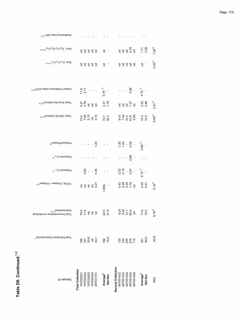
Tabl

e D

6. C

ontin

ued.

1-3

Sample ID

Total Petroleum Hydrocarbons5

Total Concentrations of Individual Hydrocarbons

6,7,15

TOTAL: Pristane + Phytane6,15

Pristane/n-C1716

Phytane/n-C1816

Pristane/Phytane16

Total: Odd No Carbons6,8,15

Total: Even No Carbons6,9,15

Carbon Preference Index (CPI)10,16

Sum: C10-C12-C146,11,15

Sum: C22-C24-C26-C286,12,15

Weathering Index (WI)13,16

Firs

t Col

lect

ion

1970

2042

1

195

79.

5

nd

-

-

-

73.

2

6.

21

11.

8

nd

nd

-

1970

2042

2

161

11.

9

nd

0.

64

-

-

7.

92

3.

76

2.

11

nd

nd

-

1970

2042

3

83.

6

nd

nd

-

-

-

5.

15

nd

-

nd

nd

-

1970

2042

5

nd

nd

nd

-

-

-

nd

nd

-

nd

nd

-

2970

3170

1

63.

1

nd

0.

21

0.

45

-

1.

20

5.

74

nd

-

nd

nd

-

Ave

rage

4

106

22.

5 <

MD

L

-

-

-

1

9.1

3.31

5

.76

17

nd

nd

-

St

d D

ev

70.

0

31.

9

-

-

-

-

30.

3

1.

78

-

-

-

-

Seco

nd C

olle

ctio

n49

7051

422

1

35

9.20

0.42

0.22

-

1.35

6.41

n

d

-

n

d

n

d

- 49

7051

423

1

44

9.44

0.29

0.19

-

1.43

7.54

n

d

-

n

d

n

d

- 49

7051

424

2

35

1

2.7

0.20

-

-

-

1

0.3

n

d

-

n

d

n

d

- 49

7051

425

2

74

5

0.4

1.16

0.07

5.66

0.55

4

1.8

7.37

5.68

n

d

5.79

- 49

7051

426

1

15

n

d

n

d

-

-

-

5.60

n

d

-

n

d

n

d

-

Ave

rage

4

181

17.

8

0.

45

0.1

0 17

-

0.6

9 17

1

4.3

3.02

4

.75

17

nd

1.

71

-

St

d D

ev

69.

5

18.

3

0.

41

-

-

-

15.

5

2.

46

-

-

2.

28

-

MD

L

53

.68.

1914

0.19

145.

0914

2.91

140.

2914

1.29

14

175Page

Tabl

e D

6. C

ontin

ued.

Foot

note

s:1

Th

e co

ncen

tratio

ns o

f the

indi

vidu

al a

lipha

tic h

ydro

carb

ons

and

the

tota

l pet

role

um h

ydro

carb

ons

wer

e de

term

ined

usi

ng e

xter

nal s

tand

ard

calc

ulat

ions

.2

W

hen

an in

divi

dual

alip

hatic

hyd

roca

rbon

was

not

det

ecte

d, it

s co

ncen

tratio

n w

as re

plac

ed b

y nd

.3

Th

e co

ncen

tratio

ns fo

r n-C

8 will

be

not r

epor

ted,

sin

ce it

was

diff

icul

t to

iden

tify

this

pea

k in

sam

ples

and

to d

eter

min

e M

DL

for n

-C8.

4

If al

l con

cent

ratio

ns a

re n

d, th

e av

erag

e is

repl

aced

with

nd.

Whe

n th

ere

is a

t lea

st o

ne n

umbe

r in

the

data

set

to b

e av

erag

ed, e

ach

nd is

repl

aced

w

ith 1

/2*M

DL,

and

an

aver

age

is c

alcu

late

d. If

this

num

eric

val

ue is

less

than

the

MD

L, th

e av

erag

e is

repl

aced

by

< M

DL;

oth

erw

ise,

the

aver

age

is th

eca

lcul

ated

val

ue. W

hen

a nu

mer

ic v

alue

is fo

und

for t

he a

vera

ge, t

he s

tand

ard

devi

atio

n is

then

det

erm

ined

usi

ng th

e sa

me

num

ber s

et u

sed

to c

alcu

late

the

aver

age.

5

D

eter

min

ed fr

om th

e to

tal p

eak

area

s in

the

chro

mat

ogra

m fr

om n

-C8 t

o n-

C40

min

us a

ny c

ontri

butio

ns fr

om th

e in

tern

al s

tand

ard

area

s.6

Th

ese

form

ulae

use

1/2

MD

L va

lues

for e

ach

anal

yte

not d

etec

ted.

7

Sum

of t

he c

once

ntra

tions

of t

he in

divi

dual

alip

hatic

hyd

roca

rbon

s n-

C9 t

hrou

gh n

-C40

plu

s th

e co

ncen

tratio

ns o

f pris

tane

and

phy

tane

.8

Th

e to

tal o

f the

con

cent

ratio

ns o

f the

alip

hatic

hyd

roca

rbon

s w

ith a

n od

d nu

mbe

r of c

arbo

n at

oms.

9

The

tota

l of t

he c

once

ntra

tions

of t

he a

lipha

tic h

ydro

carb

ons

with

an

even

num

ber o

f car

bon

atom

s. T

he c

ontri

butio

n of

n-C

8 is

not i

nclu

ded

in th

e to

tal.

10

Car

bon

Pre

fere

nce

Inde

x (C

PI)

is d

efin

ed a

s th

e ra

tio o

f the

tota

l of t

he c

once

ntra

tions

of t

he a

lipha

tic h

ydro

carb

ons

with

an

odd

num

ber o

f car

bons

to th

eto

tal c

once

ntra

tion

of th

e al

phat

ic h

ydro

carb

ons

with

an

even

car

bon

num

ber.

11Th

e to

tal o

f the

con

cent

ratio

ns o

f n-C

10, n

-C12

, and

n-C

14.

12 T

he to

tal o

f the

con

cent

ratio

ns o

f n-C

22, n

-C24

, n-C

26, a

nd n

-C28

.13

W

eath

erin

g In

dex

(WI)

is d

efin

ed a

s th

e ra

tio o

f the

tota

l con

cent

ratio

n of

n-C

10, n

-C12

, and

n-C

14 to

the

tota

l con

cent

ratio

n of

n-C

22, n

-C24

, n-C

26, a

nd n

-C28

.14

T

hese

MD

L va

lues

are

cal

cula

ted

with

the

sam

e su

mm

atio

n fo

rmul

ae a

s th

e sa

mpl

es u

sing

the

indi

vidu

al h

ydro

carb

on M

DL

valu

es.

15

The

sum

mat

ion

tota

ls fo

r the

sam

ples

are

com

pare

d w

ith c

alcu

late

d M

DL

valu

es o

btai

ned

usin

g th

e sa

me

sum

mat

ion

form

ulae

as

the

sam

ples

.W

hen

thes

e sa

mpl

e to

tals

wer

e le

ss th

an th

e to

tal M

DL,

its

valu

e w

as re

plac

ed b

y nd

. The

ave

rage

s an

d st

anda

rd d

evia

tions

for t

he to

tals

wer

etre

ated

in th

e sa

me

way

as

the

indi

vidu

al h

ydro

carb

ons;

see

foot

note

4.

16

Num

eric

al v

alue

s of

the

CP

I, W

I, an

d th

e ra

tios:

pris

tane

/n-C

17, p

hyta

ne/n

-C18

, and

pris

tane

/phy

tane

, will

be

calc

ulat

ed o

nly

whe

n th

e de

fined

qua

ntity

for e

ach

inde

x or

ratio

has

a n

umer

ic v

alue

.17

T

hese

resu

lts a

re n

ot tr

ue a

vera

ges,

inst

ead

they

are

the

ratio

s of

the

aver

ages

of t

he d

efin

ed q

uant

ities

, if t

hese

ave

rage

s ex

ist.

Page 176

Tabl

e D

7. In

divi

dual

hyd

roca

rbon

and

tota

l pet

role

um h

ydro

carb

on c

once

ntra

tions

(in

g/g

wet

wt.)

for r

ibbe

d m

usse

ls ta

ken

from

Saw

M

ill N

orth

mar

sh, a

repl

ante

d si

te.1-

3

Sample ID

Nonane (n-C9)

Decane (n-C10)

Undecane (n-C11)

Dodecane (n-C12)

Tridecane (n-C13)

Tetradecane (n-C14)

Pentadecane (n-C15)

Hexadecane (n-C16)

Heptadecane (n-C17)

Pristane

Octadecane (n-C18)

Phytane

Nonadecane (n-C19)

Eicosane (n-C20)

Heneicosane (n-C21)

Docosane (n-C22)

Tricosane (n-C23)

Firs

t Col

lect

ion

1970

2040

10.

66nd

ndnd

ndnd

0.12

0.14

0.29

0.11

ndnd

0.23

nd1.

22nd

nd19

7020

402

ndnd

ndnd

ndnd

nd0.

110.

230.

16nd

0.12

0.18

nd1.

62nd

nd19

7020

409

ndnd

ndnd

ndnd

ndnd

0.20

ndnd

nd0.

21nd

1.54

ndnd

1970

2041

50.

65nd

ndnd

ndnd

ndnd

0.23

0.15

ndnd

0.12

nd1.

45nd

nd29

7031

702

ndnd

ndnd

ndnd

ndnd

0.13

ndnd

ndnd

ndnd

ndnd

Ave

rage

40.

33nd

ndnd

ndnd

< M

DL

< M

DL

0.22

0.11

nd<

MD

L0.

16nd

1.20

ndnd

Std

Dev

0.29

--

--

--

-0.

060.

05-

-0.

07-

0.59

--

Seco

nd C

olle

ctio

n49

7051

405

ndnd

ndnd

ndnd

ndnd

0.96

ndnd

ndnd

0.24

2.52

1.01

4.53

4970

5140

6nd

ndnd

ndnd

ndnd

nd0.

89nd

nd0.

130.

12nd

2.35

0.80

3.08

4970

5140

70.

52nd

ndnd

nd0.

230.

170.

120.

780.

300.

150.

300.

290.

383.

792.

073.

8749

7051

409

ndnd

ndnd

ndnd

ndnd

0.84

ndnd

ndnd

ndnd

ndnd

4970

5141

0nd

ndnd

ndnd

ndnd

nd0.

89nd

nd0.

120.

17nd

ndnd

nd

Ave

rage

4<

MD

Lnd

ndnd

nd<

MD

L<

MD

L<

MD

L0.

870.

10<

MD

L0.

130.

14<

MD

L1.

810.

912.

79St

d D

ev-

--

--

--

-0.

070.

11-

0.10

0.10

-1.

580.

711.

51

MD

L0.

240.

060.

120.

120.

110.

110.

110.

090.

080.

100.

100.

100.

110.

210.

380.

682.

47

177Page

Tabl

e D

7. C

ontin

ued.

1-3

Sample ID

Tetracosane (n-C24)

Pentacosane (n-C25)

Hexacosane (n-C26)

Heptacosane (n-C27)

Octacosane (n-C28)

Nonacosane (n-C29)

Triacontane (n-C30)

n-Hentriacontane (n-C31)

Dotriacontane (n-C32)

Tritriacontane (n-C33)

Tetratriacontane (n-C34)

Pentatriacontane (n-C35)

Hexatriacontane (n-C36)

Heptatriacontane (n-C37)

Octatriacontane (n-C38)

Nonatriacontane (n-C39)

Tetracontane (n-C40)

Firs

t Col

lect

ion

1970

2040

1nd

nd0.

19nd

ndnd

ndnd

3.13

3.65

0.32

0.43

0.39

0.41

0.32

0.24

0.15

1970

2040

2nd

ndnd

ndnd

ndnd

0.55

1.27

0.22

0.40

0.45

0.43

0.44

0.34

0.25

0.16

1970

2040

9nd

ndnd

ndnd

ndnd

0.40

0.33

0.41

0.46

0.52

0.50

0.49

0.39

0.29

0.18

1970

2041

5nd

ndnd

0.21

0.39

ndnd

0.52

0.70

0.70

0.73

0.80

0.76

0.74

0.59

0.44

0.27

2970

3170

2nd

ndnd

ndnd

ndnd

0.14

nd0.

12nd

ndnd

ndnd

0.10

0.12

Ave

rage

4nd

nd<

MD

L<

MD

L<

MD

Lnd

nd0.

341.

101.

020.

390.

450.

430.

430.

340.

260.

18St

d D

ev-

--

--

--

0.23

1.22

1.49

0.25

0.27

0.26

0.23

0.20

0.12

0.06

Seco

nd C

olle

ctio

n49

7051

405

1.33

0.63

0.20

0.61

1.04

8.55

nd0.

420.

720.

20nd

nd0.

140.

180.

160.

10nd

4970

5140

6nd

ndnd

ndnd

ndnd

0.12

ndnd

ndnd

ndnd

ndnd

nd49

7051

407

ndnd

ndnd

ndnd

nd0.

603.

310.

29nd

0.19

0.11

nd0.

140.

08nd

4970

5140

9nd

ndnd

ndnd

ndnd

nd0.

17nd

ndnd

ndnd

ndnd

nd49

7051

410

ndnd

ndnd

ndnd

nd0.

301.

600.

14nd

ndnd

ndnd

ndnd

Ave

rage

40.

38<

MD

L<

MD

L0.

150.

291.

93nd

0.30

1.18

0.14

nd<

MD

L<

MD

L<

MD

L0.

09<

MD

Lnd

Std

Dev

0.53

--

0.26

0.42

3.70

-0.

221.

340.

10-

--

-0.

06-

-

MD

L0.

290.

270.

110.

080.

200.

560.

480.

110.

140.

110.

090.

100.

100.

180.

080.

060.

06

Page 178

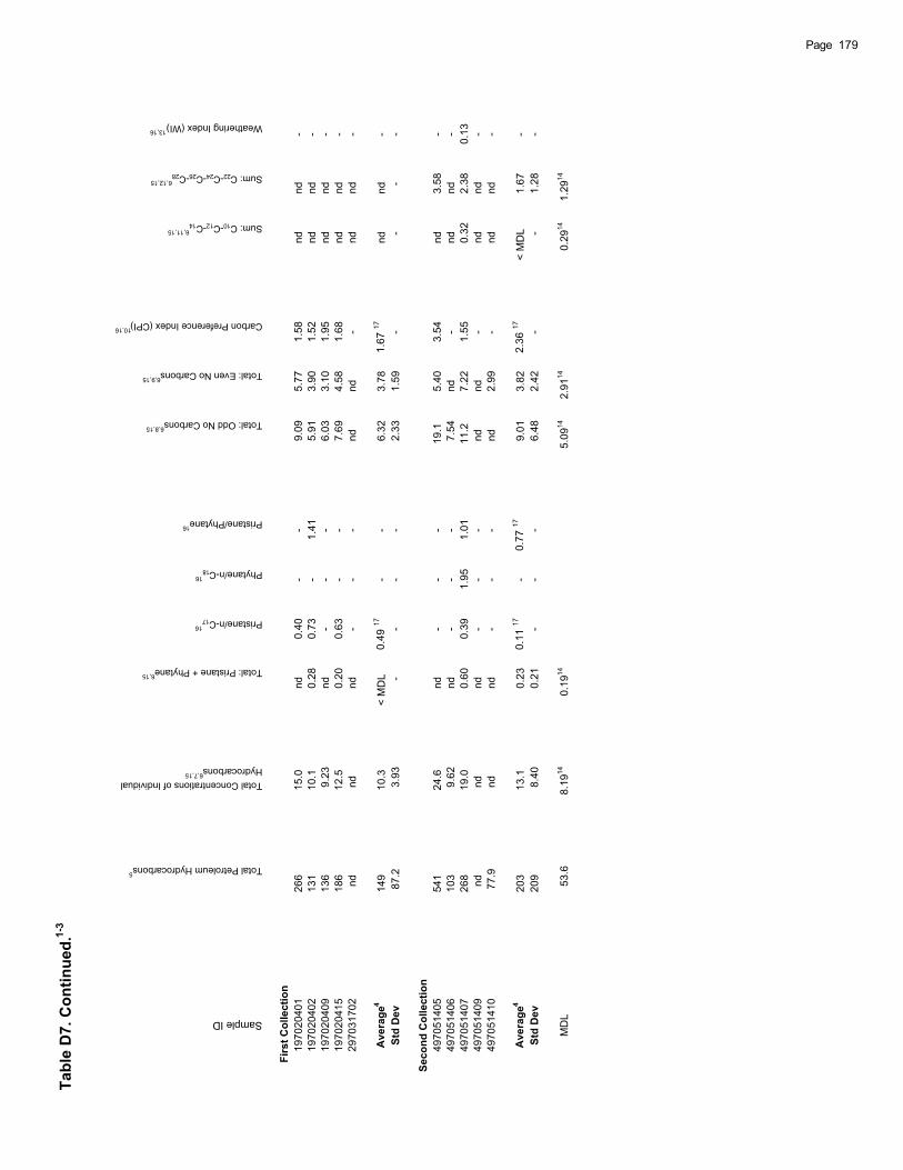
Tabl

e D

7. C

ontin

ued.

1-3

Sample ID

Total Petroleum Hydrocarbons5

Total Concentrations of Individual Hydrocarbons

6,7,15

Total: Pristane + Phytane6,15

Pristane/n-C1716

Phytane/n-C1816

Pristane/Phytane16

Total: Odd No Carbons6,8,15

Total: Even No Carbons6,9,15

Carbon Preference Index (CPI)10,16

Sum: C10-C12-C146,11,15

Sum: C22-C24-C26-C286,12,15

Weathering Index (WI)13,16

Firs

t Col

lect

ion

1970

2040

1

266

15.

0

nd

0.

40

-

-

9.

09

5.

77

1.

58

nd

nd

-

1970

2040

2

131

10.

1

0.

28

0.

73

-

1.

41

5.

91

3.

90

1.

52

nd

nd

-

1970

2040

9

136

9.

23

nd

-

-

-

6.

03

3.

10

1.

95

nd

nd

-

1970

2041

5

186

12.

5

0.

20

0.

63

-

-

7.

69

4.

58

1.

68

nd

nd

-

2970

3170

2

nd

nd

nd

-

-

-

nd

nd

-

nd

nd

-

Ave

rage

4

149

10.

3 <

MD

L

0

.49

17

-

-

6.

32

3.

78

1.6

7 17

n

d

n

d

-

Std

Dev

8

7.2

3.93

-

-

-

-

2.33

1.59

-

-

-

-

Seco

nd C

olle

ctio

n49

7051

405

5

41

2

4.6

n

d

-

-

-

1

9.1

5.40

3.54

n

d

3.58

- 49

7051

406

1

03

9.62

n

d

-

-

-

7.54

n

d

-

n

d

n

d

- 49

7051

407

2

68

1

9.0

0.60

0.39

1.95

1.01

1

1.2

7.22

1.55

0.32

2.38

0.13

4970

5140

9

nd

nd

nd

-

-

-

nd

nd

-

nd

nd

-

4970

5141

0

77.

9

nd

nd

-

-

-

nd

2.

99

-

nd

nd

-

Ave

rage

4

203

13.

1

0.

23

0.1

1 17

-

0.7

7 17

9.01

3.82

2

.36

17 <

MD

L

1.67

-

Std

Dev

2

09

8.40

0.21

-

-

-

6.48

2.42

-

-

1.28

-

MD

L

53

.68.

1914

0.19

145.

0914

2.91

140.

2914

1.29

14

179Page

Tabl

e D

7. C

ontin

ued.

Foot

note

s:1

Th

e co

ncen

tratio

ns o

f the

indi

vidu

al a

lipha

tic h

ydro

carb

ons

and

the

tota

l pet

role

um h

ydro

carb

ons

wer

e de

term

ined

usi

ng e

xter

nal s

tand

ard

calc

ulat

ions

.2

W

hen

an in

divi

dual

alip

hatic

hyd

roca

rbon

was

not

det

ecte

d, it

s co

ncen

tratio

n w

as re

plac

ed b

y nd

.3

Th

e co

ncen

tratio

ns fo

r n-C

8 will

be

not r

epor

ted,

sin

ce it

was

diff

icul

t to

iden

tify

this

pea

k in

sam

ples

and

to d

eter

min

e M

DL

for n

-C8.

4

If al

l con

cent

ratio

ns a

re n

d, th

e av

erag

e is

repl

aced

with

nd.

Whe

n th

ere

is a

t lea

st o

ne n

umbe

r in

the

data

set

to b

e av

erag

ed, e

ach

nd is

repl

aced

w

ith 1

/2*M

DL,

and

an

aver

age

is c

alcu

late

d. If

this

num

eric

val

ue is

less

than

the

MD

L, th

e av

erag

e is

repl

aced

by

< M

DL;

oth

erw

ise,

the

aver

age

is th

eca

lcul

ated

val

ue. W

hen

a nu

mer

ic v

alue

is fo

und

for t

he a

vera

ge, t

he s

tand

ard

devi

atio

n is

then

det

erm

ined

usi

ng th

e sa

me

num

ber s

et u

sed

to c

alcu

late

the

aver

age.

5

D

eter

min

ed fr

om th

e to

tal p

eak

area

s in

the

chro

mat

ogra

m fr

om n

-C8 t

o n-

C40

min

us a

ny c

ontri

butio

ns fr

om th

e in

tern

al s

tand

ard

area

s.6

Th

ese

form

ulae

use

1/2

MD

L va

lues

for e

ach

anal

yte

not d

etec

ted.

7

Sum

of t

he c

once

ntra

tions

of t

he in

divi

dual

alip

hatic

hyd

roca

rbon

s n-

C9 t

hrou

gh n

-C40

plu

s th

e co

ncen

tratio

ns o

f pris

tane

and

phy

tane

.8

Th

e to

tal o

f the

con

cent

ratio

ns o

f the

alip

hatic

hyd

roca

rbon

s w

ith a

n od

d nu

mbe

r of c

arbo

n at

oms.

9

The

tota

l of t

he c

once

ntra

tions

of t

he a

lipha

tic h

ydro

carb

ons

with

an

even

num

ber o

f car

bon

atom

s. T

he c

ontri

butio

n of

n-C

8 is

not i

nclu

ded

in th

e to

tal.

10

Car

bon

Pre

fere

nce

Inde

x (C

PI)

is d

efin

ed a

s th

e ra

tio o

f the

tota

l of t

he c

once

ntra

tions

of t

he a

lipha

tic h

ydro

carb

ons

with

an

odd

num

ber o

f car

bons

to th

eto

tal c

once

ntra

tion

of th

e al

phat

ic h

ydro

carb

ons

with

an

even

car

bon

num

ber.

11Th

e to

tal o

f the

con

cent

ratio

ns o

f n-C

10, n

-C12

, and

n-C

14.

12 T

he to

tal o

f the

con

cent

ratio

ns o

f n-C

22, n

-C24

, n-C

26, a

nd n

-C28

.13

W

eath

erin

g In

dex

(WI)

is d

efin

ed a

s th

e ra

tio o

f the

tota

l con

cent

ratio

n of

n-C

10, n

-C12

, and

n-C

14 to

the

tota

l con

cent

ratio

n of

n-C

22, n

-C24

, n-C

26, a

nd n

-C28

.14

T

hese

MD

L va

lues

are

cal

cula

ted

with

the

sam

e su

mm

atio

n fo

rmul

ae a

s th

e sa

mpl

es u

sing

the

indi

vidu

al h

ydro

carb

on M

DL

valu

es.

15

The

sum

mat

ion

tota

ls fo

r the

sam

ples

are

com

pare

d w

ith c

alcu

late

d M

DL

valu

es o

btai

ned

usin

g th

e sa

me

sum

mat

ion

form

ulae

as

the

sam

ples

.W

hen

thes

e sa

mpl

e to

tals

wer

e le

ss th

an th

e to

tal M

DL,

its

valu

e w

as re

plac

ed b

y nd

. The

ave

rage

s an

d st

anda

rd d

evia

tions

for t

he to

tals

wer

etre

ated

in th

e sa

me

way

as

the

indi

vidu

al h

ydro

carb

ons;

see

foot

note

4.

16

Num

eric

al v

alue

s of

the

CP

I, W

I, an

d th

e ra

tios:

pris

tane

/n-C

17, p

hyta

ne/n

-C18

, and

pris

tane

/phy

tane

, will

be

calc

ulat

ed o

nly

whe

n th

e de

fined

qua

ntity

for e

ach

inde

x or

ratio

has

a n

umer

ic v

alue

.17

T

hese

resu

lts a

re n

ot tr

ue a

vera

ges,

inst

ead

they

are

the

ratio

s of

the

aver

ages

of t

he d

efin

ed q

uant

ities

, if t

hese

ave

rage

s ex

ist.

Page 180

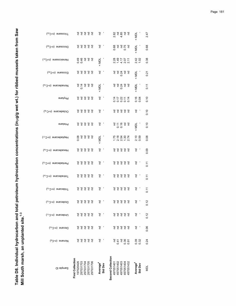
Tabl

e D

8. In

divi

dual

hyd

roca

rbon

and

tota

l pet

role

um h

ydro

carb

on c

once

ntra

tions

(in

g/g

wet

wt.)

for r

ibbe

d m

usse

ls ta

ken

from

Saw

M

ill S

outh

mar

sh, a

n un

plan

ted

site

.1-3

Sample ID

Nonane (n-C9)

Decane (n-C10)

Undecane (n-C11)

Dodecane (n-C12)

Tridecane (n-C13)

Tetradecane (n-C14)

Pentadecane (n-C15)

Hexadecane (n-C16)

Heptadecane (n-C17)

Pristane

Octadecane (n-C18)

Phytane

Nonadecane (n-C19)

Eicosane (n-C20)

Heneicosane (n-C21)

Docosane (n-C22)

Tricosane (n-C23)

Firs

t Col

lect

ion

1970

2042

6nd

ndnd

ndnd

ndnd

nd0.

08nd

ndnd

ndnd

0.49

ndnd

2970

3170

3nd

ndnd

ndnd

ndnd

ndnd

ndnd

nd0.

14nd

0.46

ndnd

2970

3170

4nd

ndnd

ndnd

ndnd

ndnd

ndnd

ndnd

ndnd

ndnd

2970

3170

5nd

ndnd

ndnd

ndnd

ndnd

ndnd

ndnd

ndnd

ndnd

2970

3170

6nd

ndnd

ndnd

ndnd

ndnd

ndnd

ndnd

ndnd

ndnd

Ave

rage

4nd

ndnd

ndnd

ndnd

nd<

MD

Lnd

ndnd

< M

DL

nd<

MD

Lnd

ndSt

d D

ev-

--

--

--

--

--

--

--

--

Seco

nd C

olle

ctio

n49

7051

401

ndnd

ndnd

ndnd

ndnd

1.75

ndnd

0.14

ndnd

2.28

0.68

2.82

4970

5140

20.

41nd

ndnd

ndnd

ndnd

2.18

0.11

nd0.

17nd

nd1.

49nd

nd49

7051

403

ndnd

ndnd

ndnd

ndnd

2.54

0.16

nd0.

220.

240.

244.

17nd

4.85

4970

5140

40.

36nd

ndnd

ndnd

ndnd

1.30

ndnd

0.11

ndnd

2.07

0.75

nd49

7051

432

0.91

ndnd

ndnd

ndnd

nd2.

74nd

nd0.

14nd

nd2.

11nd

nd

Ave

rage

40.

39nd

ndnd

ndnd

ndnd

2.10

< M

DL

nd0.

16<

MD

L<

MD

L2.

42<

MD

L<

MD

LSt

d D

ev0.

32-

--

--

--

0.59

--

0.04

--

1.02

--

MD

L0.

240.

060.

120.

120.

110.

110.

110.

090.

080.

100.

100.

100.

110.

210.

380.

682.

47

181Page

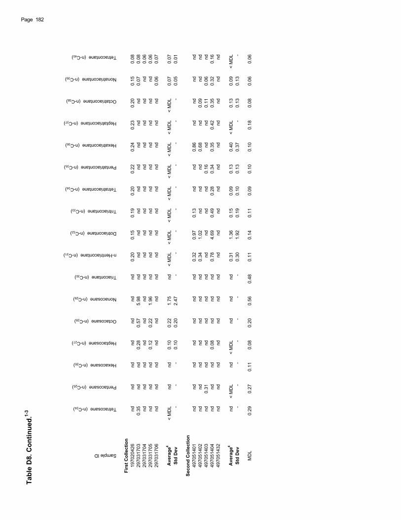
Tabl

e D

8. C

ontin

ued.

1-3

Sample ID

Tetracosane (n-C24)

Pentacosane (n-C25)

Hexacosane (n-C26)

Heptacosane (n-C27)

Octacosane (n-C28)

Nonacosane (n-C29)

Triacontane (n-C30)

n-Hentriacontane (n-C31)

Dotriacontane (n-C32)

Tritriacontane (n-C33)

Tetratriacontane (n-C34)

Pentatriacontane (n-C35)

Hexatriacontane (n-C36)

Heptatriacontane (n-C37)

Octatriacontane (n-C38)

Nonatriacontane (n-C39)

Tetracontane (n-C40)

Firs

t Col

lect

ion

1970

2042

6nd

ndnd

ndnd

ndnd

0.20

0.15

0.19

0.20

0.22

0.24

0.23

0.20

0.15

0.08

2970

3170

30.

35nd

nd0.

280.

575.

98nd

ndnd

ndnd

ndnd

ndnd

0.07

0.08

2970

3170

4nd

ndnd

ndnd

ndnd

ndnd

ndnd

ndnd

ndnd

nd0.

0629

7031

705

ndnd

nd0.

120.

221.

96nd

ndnd

ndnd

ndnd

ndnd

nd0.

0629

7031

706

ndnd

ndnd

ndnd

ndnd

ndnd

ndnd

ndnd

nd0.

060.

07

Ave

rage

4<

MD

Lnd

nd0.

100.

221.

75nd

< M

DL

< M

DL

< M

DL

< M

DL

< M

DL

< M

DL

< M

DL

< M

DL

0.07

0.07

Std

Dev

--

-0.

100.

202.

47-

--

--

--

--

0.05

0.01

Seco

nd C

olle

ctio

n49

7051

401

ndnd

ndnd

ndnd

nd0.

320.

970.

13nd

nd0.

86nd

ndnd

nd49

7051

402

ndnd

ndnd

ndnd

nd0.

341.

02nd

ndnd

0.68

nd0.

09nd

nd49

7051

403

nd0.

31nd

ndnd

ndnd

ndnd

ndnd

0.16

ndnd

0.11

0.06

nd49

7051

404

ndnd

nd0.

08nd

ndnd

0.78

4.69

0.49

0.28

0.34

0.35

0.42

0.35

0.32

0.16

4970

5143

2nd

ndnd

ndnd

ndnd

ndnd

ndnd

ndnd

ndnd

ndnd

Ave

rage

4nd

< M

DL

nd<

MD

Lnd

ndnd

0.31

1.36

0.15

0.09

0.13

0.40

< M

DL

0.13

0.09

< M

DL

Std

Dev

--

--

--

-0.

301.

920.

190.

100.

130.

37-

0.13

0.13

-

MD

L0.

290.

270.

110.

080.

200.

560.

480.

110.

140.

110.

090.

100.

100.

180.

080.

060.

06

Page 182

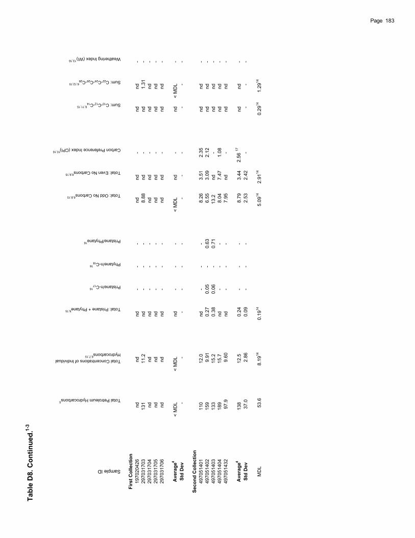
Tabl

e D

8. C

ontin

ued.

1-3

Sample ID

Total Petroleum Hydrocarbons5

Total Concentrations of Individual Hydrocarbons

6,7,15

Total: Pristane + Phytane6,15

Pristane/n-C1716

Phytane/n-C1816

Pristane/Phytane16

Total: Odd No Carbons6,8,15

Total: Even No Carbons6,9,15

Carbon Preference Index (CPI)10,16

Sum: C10-C12-C146,11,15

Sum: C22-C24-C26-C286,12,15

Weathering Index (WI)13,16

Firs

t Col

lect

ion

1970

2042

6

nd

nd

nd

-

-

-

nd

nd

-

nd

nd

-

2970

3170

3

131

11.

2

nd

-

-

-

8.

88

nd

-

nd

1.

31

-

2970

3170

4

nd

nd

nd

-

-

-

nd

nd

-

nd

nd

-

2970

3170

5

nd

nd

nd

-

-

-

nd

nd

-

nd

nd

-

2970

3170

6

nd

nd

nd

-

-

-

nd

nd

-

nd

nd

-

Ave

rage

4

< M

DL

< M

DL

nd

-

-

-

< M

DL

nd

-

nd

<

MD

L

-

Std

Dev

-

-

-

-

-

-

-

-

-

-

-

-

Seco

nd C

olle

ctio

n49

7051

401

1

10

1

2.0

n

d

-

-

-

8.26

3.51

2.35

n

d

n

d

- 49

7051

402

1

59

9.91

0.27

0.05

-

0.63

6.55

3.09

2.12

n

d

n

d

- 49

7051

403

1

33

1

5.2

0.38

0.06

-

0.71

1

3.2

n

d

-

n

d

n

d

- 49

7051

404

1

89

1

5.7

n

d

-

-

-

8.04

7.47

1.08

n

d

n

d

- 49

7051

432

9

7.9

9.60

n

d

-

-

-

7.95

n

d

-

n

d

n

d

-

Ave

rage

4

138

12.

5

0.

24

-

-

-

8.

79

3.

44

2.5

6 17

n

d

n

d

-

Std

Dev

3

7.0

2.86

0.09

-

-

-

2.53

2.42

-

-

-

-

MD

L

53

.68.

1914

0.19

145.

0914

2.91

140.

2914

1.29

14

183Page

Tabl

e D

8. C

ontin

ued.

Foot

note

s:1

Th

e co

ncen

tratio

ns o

f the

indi

vidu

al a

lipha

tic h

ydro

carb

ons

and

the

tota

l pet

role

um h

ydro

carb

ons

wer

e de

term

ined

usi

ng e

xter

nal s

tand

ard

calc

ulat

ions

.2

W

hen

an in

divi

dual

alip

hatic

hyd

roca

rbon

was

not

det

ecte

d, it

s co

ncen

tratio

n w

as re

plac

ed b

y nd

.3

Th

e co

ncen

tratio

ns fo

r n-C

8 will

be

not r

epor

ted,

sin

ce it

was

diff

icul

t to

iden

tify

this

pea

k in

sam

ples

and

to d

eter

min

e M

DL

for n

-C8.

4

If al

l con

cent

ratio

ns a

re n

d, th

e av

erag

e is

repl

aced

with

nd.

Whe

n th

ere

is a

t lea

st o

ne n

umbe

r in

the

data

set

to b

e av

erag

ed, e

ach

nd is

repl

aced

w

ith 1

/2*M

DL,

and

an

aver

age

is c

alcu

late

d. If

this

num

eric

val

ue is

less

than

the

MD

L, th

e av

erag

e is

repl

aced

by

< M

DL;

oth

erw

ise,

the

aver

age

is th

eca

lcul

ated

val

ue. W

hen

a nu

mer

ic v

alue

is fo

und

for t

he a

vera

ge, t

he s

tand

ard

devi

atio

n is

then

det

erm

ined

usi

ng th

e sa

me

num

ber s

et u

sed

to c

alcu

late

the

aver

age.

5

D

eter

min

ed fr

om th

e to

tal p

eak

area

s in

the

chro

mat

ogra

m fr

om n

-C8 t

o n-

C40

min

us a

ny c

ontri

butio

ns fr

om th

e in

tern

al s

tand

ard

area

s.6

Th

ese

form

ulae

use

1/2

MD

L va

lues

for e

ach

anal

yte

not d

etec

ted.

7

Sum

of t

he c

once

ntra

tions

of t

he in

divi

dual

alip

hatic

hyd

roca

rbon

s n-

C9 t

hrou

gh n

-C40

plu

s th

e co

ncen

tratio

ns o

f pris

tane

and

phy

tane

.8

Th

e to

tal o

f the

con

cent

ratio

ns o

f the

alip

hatic

hyd

roca

rbon

s w

ith a

n od

d nu

mbe

r of c

arbo

n at

oms.

9

The

tota

l of t

he c

once

ntra

tions

of t

he a

lipha

tic h

ydro

carb

ons

with

an

even

num

ber o

f car

bon

atom

s. T

he c

ontri

butio

n of

n-C

8 is

not i

nclu

ded

in th

e to

tal.

10

Car

bon

Pre

fere

nce

Inde

x (C

PI)

is d

efin

ed a

s th

e ra

tio o

f the

tota

l of t

he c

once

ntra

tions

of t

he a

lipha

tic h

ydro

carb

ons

with

an

odd

num

ber o

f car

bons

to th

eto

tal c

once

ntra

tion

of th

e al

phat

ic h

ydro

carb

ons

with

an

even

car

bon

num

ber.

11Th

e to

tal o

f the

con

cent

ratio

ns o

f n-C

10, n

-C12

, and

n-C

14.

12 T

he to

tal o

f the

con

cent

ratio

ns o

f n-C

22, n

-C24

, n-C

26, a

nd n

-C28

.13

W

eath

erin

g In

dex

(WI)

is d

efin

ed a

s th

e ra

tio o

f the

tota

l con

cent

ratio

n of

n-C

10, n

-C12

, and

n-C

14 to

the

tota

l con

cent

ratio

n of

n-C

22, n

-C24

, n-C

26, a

nd n

-C28

.14

T

hese

MD

L va

lues

are

cal

cula

ted

with

the

sam

e su

mm

atio

n fo

rmul

ae a

s th

e sa

mpl

es u

sing

the

indi

vidu

al h

ydro

carb

on M

DL

valu

es.

15

The

sum

mat

ion

tota

ls fo

r the

sam

ples

are

com

pare

d w

ith c

alcu

late

d M

DL

valu

es o

btai

ned

usin

g th

e sa

me

sum

mat

ion

form

ulae

as

the

sam

ples

.W

hen

thes

e sa

mpl

e to

tals

wer

e le

ss th

an th

e to

tal M

DL,

its

valu

e w

as re

plac

ed b

y nd

. The

ave

rage

s an

d st

anda

rd d

evia

tions

for t

he to

tals

wer

etre

ated

in th

e sa

me

way

as

the

indi

vidu

al h

ydro

carb

ons;

see

foot

note

4.

16

Num

eric

al v

alue

s of

the

CP

I, W

I, an

d th

e ra

tios:

pris

tane

/n-C

17, p

hyta

ne/n

-C18

, and

pris

tane

/phy

tane

, will

be

calc

ulat

ed o

nly

whe

n th

e de

fined

qua

ntity

for e

ach

inde

x or

ratio

has

a n

umer

ic v

alue

.17

T

hese

resu

lts a

re n

ot tr

ue a

vera

ges,

inst

ead

they

are

the

ratio

s of

the

aver

ages

of t

he d

efin

ed q

uant

ities

, if t

hese

ave

rage

s ex

ist.

Page 184

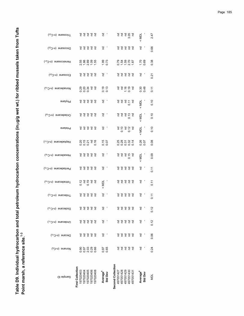
Tabl

e D

9. In

divi

dual

hyd

roca

rbon

and

tota

l pet

role

um h

ydro

carb

on c

once

ntra

tions

(in

g/g

wet

wt.)

for r

ibbe

d m

usse

ls ta

ken

from

Tuf

ts

Poin

t mar

sh, a

refe

renc

e si

te.1-

3

Sample ID

Nonane (n-C9)

Decane (n-C10)

Undecane (n-C11)

Dodecane (n-C12)

Tridecane (n-C13)

Tetradecane (n-C14)

Pentadecane (n-C15)

Hexadecane (n-C16)

Heptadecane (n-C17)

Pristane

Octadecane (n-C18)

Phytane

Nonadecane (n-C19)

Eicosane (n-C20)

Heneicosane (n-C21)

Docosane (n-C22)

Tricosane (n-C23)

Firs

t Col

lect

ion

1970

2040

30.

90nd

ndnd

nd0.

12nd

nd0.

20nd

ndnd

0.29

nd2.

55nd

nd19

7020

404

0.97

ndnd

ndnd

ndnd

nd0.

15nd

ndnd

0.20

nd1.

86nd

nd19

7020

405

2.03

ndnd

ndnd

0.19

ndnd

0.21

ndnd

nd0.

34nd

2.89

ndnd

1970

2040

60.

29nd

ndnd

ndnd

ndnd

ndnd

ndnd

ndnd

1.09

ndnd

1970

2040

80.

66nd

ndnd

ndnd

ndnd

0.16

ndnd

ndnd

nd1.

55nd

nd

Ave

rage

40.

97nd

ndnd

nd<

MD

Lnd

nd0.

15nd

ndnd

0.19

nd1.

99nd

ndSt

d D

ev0.

65-

--

--

--

0.07

--

-0.

13-

0.73

--

Sec

ond

Col

lect

ion

4970

5142

7nd

ndnd

ndnd

ndnd

nd0.

25nd

ndnd

ndnd

0.79

ndnd

4970

5142

8nd

ndnd

ndnd

ndnd

nd0.

280.

10nd

ndnd

nd1.

54nd

nd49

7051

429

ndnd

ndnd

ndnd

ndnd

0.31

ndnd

nd1.

16nd

1.59

ndnd

4970

5143

0nd

ndnd

ndnd

ndnd

0.15

0.32

0.12

0.13

0.11

0.19

nd2.

70nd

3.05

4970

5143

1nd

ndnd

ndnd

ndnd

nd0.

14nd

ndnd

ndnd

1.87

ndnd

Ave

rage

4nd

ndnd

ndnd

ndnd

< M

DL

0.26

< M

DL

< M

DL

< M

DL

0.30

nd1.

70nd

< M

DL

Std

Dev

--

--

--

--

0.07

--

-0.

48-

0.69

--

MD

L0.

240.

060.

120.

120.

110.

110.

110.

090.

080.

100.

100.

100.

110.

210.

380.

682.

47

185Page

Tabl

e D

9. C

ontin

ued.

1-3

Sample ID

Tetracosane (n-C24)

Pentacosane (n-C25)

Hexacosane (n-C26)

Heptacosane (n-C27)

Octacosane (n-C28)

Nonacosane (n-C29)

Triacontane (n-C30)

n-Hentriacontane (n-C31)

Dotriacontane (n-C32)

Tritriacontane (n-C33)

Tetratriacontane (n-C34)

Pentatriacontane (n-C35)

Hexatriacontane (n-C36)

Heptatriacontane (n-C37)

Octatriacontane (n-C38)

Nonatriacontane (n-C39)

Tetracontane (n-C40)

Firs

t Col

lect

ion

1970

2040

3nd

nd0.

14nd

ndnd

nd1.

526.

130.

430.

800.

890.

890.

810.

680.

500.

3119

7020

404

0.47

nd0.

130.

401.

009.

82nd

0.84

0.41

0.46

0.60

0.68

0.68

0.65

0.55

0.41

0.25

1970

2040

50.

48nd

0.14

0.44

1.97

ndnd

0.55

0.68

0.69

0.77

0.86

0.87

0.80

0.68

0.50

0.31

1970

2040

6nd

ndnd

ndnd

ndnd

0.60

1.31

0.60

0.40

0.43

0.43

0.40

0.33

0.24

0.15

1970

2040

8nd

nd0.

15nd

ndnd

nd0.

812.

240.

220.

480.

500.

460.

470.

350.

260.

16

Ave

rage

4<

MD

Lnd

0.12

0.19

0.66

2.19

nd0.

862.

150.

480.

610.

670.

670.

630.

520.

380.

24St

d D

ev-

-0.

040.

210.

834.

27-

0.39

2.33

0.18

0.18

0.21

0.22

0.19

0.17

0.13

0.08

Sec

ond

Col

lect

ion

4970

5142

7nd

ndnd

ndnd

ndnd

ndnd

ndnd

ndnd

nd0.

120.

07nd

4970

5142

8nd

ndnd

0.16

nd0.

79nd

ndnd

ndnd

0.12

0.12

nd0.

140.

08nd

4970

5142

9nd

ndnd

ndnd

ndnd

0.13

ndnd

ndnd

0.11

nd0.

130.

08nd

4970

5143

0nd

ndnd

ndnd

ndnd

ndnd

ndnd

nd0.

10nd

0.12

0.07

nd49

7051

431

ndnd

ndnd

ndnd

ndnd

ndnd

ndnd

ndnd

ndnd

nd

Ave

rage

4nd

ndnd

< M

DL

nd<

MD

Lnd

< M

DL

ndnd

nd<

MD

L<

MD

Lnd

0.11

0.07

ndSt

d D

ev-

--

--

--

--

--

--

-0.

040.

02-

MD

L0.

290.

270.

110.

080.

200.

560.

480.

110.

140.

110.

090.

100.

100.

180.

080.

060.

06

Page 186

Tabl

e D

9. C

ontin

ued.

1-3

Sample ID

Total Petroleum Hydrocarbons5

Total Concentrations of Individual Hydrocarbons

6,7,15

Total: Pristane + Phytane6,15

Pristane/n-C1716

Phytane/n-C1816

Pristane/Phytane16

Total: Odd No Carbons6,8,15

Total: Even No Carbons6,9,15

Carbon Preference Index (CPI)10,16

Sum: C10-C12-C146,11,15

Sum: C22-C24-C26-C286,12,15

Weathering Index (WI)13,16

Firs

t Col

lect

ion

1970

2040

3

260

20.

2

nd

-

-

-

9.

95

10.

2

0.

98

nd

nd

-

1970

2040

4

288

23.

1

nd

-

-

-

18.

0

5.

02

3.

58

nd

1.

95

-

1970

2040

5

370

18.

2

nd

-

-

-

11.

1

6.

96

1.

60

nd

2.

93

-

1970

2040

6

96.

2

9.

55

nd

-

-

-

5.

60

3.

85

1.

46

nd

nd

-

1970

2040

8

158

11.

7

nd

-

-

-

6.

54

5.

02

1.

30

nd

nd

-

Ave

rage

4

235

16.

5

nd

-

-

-

10.

2

6.

21

1.6

5 17

n

d

1.40

-

Std

Dev

1

08

5.75

-

-

-

-

4.90

2.49

-

-

1.01

-

Sec

ond

Col

lect

ion

4970

5142

7

99.

8

nd

nd

-

-

-

nd

nd

-

nd

nd

-

4970

5142

8

143

nd

nd

0.

37

-

-

nd

nd

-

nd

nd

-

4970

5142

9

118

nd

nd

-

-

-

5.

44

nd

-

nd

nd

-

4970

5143

0

185

9.

32

0.

23

0.

38

0.

90

1.

08

7.

33

nd

-

nd

nd

-

4970

5143

1

69.

9

nd

nd

-

-

-

nd

nd

-

nd

nd

-

Ave

rage

4

123

< M

DL

< M

DL

-

-

-

< M

DL

nd

-

nd

nd

-

St

d D

ev

43.

7

-

-

-

-

-

-

-

-

-

-

-

MD

L

53

.68.

1914

0.19

145.

0914

2.91

140.

2914

1.29

14

187Page

Tabl

e D

9. C

ontin

ued.

Foot

note

s:1

Th

e co

ncen

tratio

ns o

f the

indi

vidu

al a

lipha

tic h

ydro

carb

ons

and

the

tota

l pet

role

um h

ydro

carb

ons

wer

e de

term

ined

usi

ng e

xter

nal s

tand

ard

calc

ulat

ions

.2

W

hen

an in

divi

dual

alip

hatic

hyd

roca

rbon

was

not

det

ecte

d, it

s co

ncen

tratio

n w

as re

plac

ed b

y nd

.3

Th

e co

ncen

tratio

ns fo

r n-C

8 will

be

not r

epor

ted,

sin

ce it

was

diff

icul

t to

iden

tify

this

pea

k in

sam

ples

and

to d

eter

min

e M

DL

for n

-C8.

4

If al

l con

cent

ratio

ns a

re n

d, th

e av

erag

e is

repl

aced

with

nd.

Whe

n th

ere

is a

t lea

st o

ne n

umbe

r in

the

data

set

to b

e av

erag

ed, e

ach

nd is

repl

aced

w

ith 1

/2*M

DL,

and

an

aver

age

is c

alcu

late

d. If

this

num

eric

val

ue is

less

than

the

MD

L, th

e av

erag

e is

repl

aced

by

< M

DL;

oth

erw

ise,

the

aver

age

is th

eca

lcul

ated

val

ue. W

hen

a nu

mer

ic v

alue

is fo

und

for t

he a

vera

ge, t

he s

tand

ard

devi

atio

n is

then

det

erm

ined

usi

ng th

e sa

me

num

ber s

et u

sed

to c

alcu

late

the

aver

age.

5

D

eter

min

ed fr

om th

e to

tal p

eak

area

s in

the

chro

mat

ogra

m fr

om n

-C8 t

o n-

C40

min

us a

ny c

ontri

butio

ns fr

om th

e in

tern

al s

tand

ard

area

s.6

Th

ese

form

ulae

use

1/2

MD

L va

lues

for e

ach

anal

yte

not d

etec

ted.

7

Sum

of t

he c

once

ntra

tions

of t

he in

divi

dual

alip

hatic

hyd

roca

rbon

s n-

C9 t

hrou

gh n

-C40

plu

s th

e co

ncen

tratio

ns o

f pris

tane

and

phy

tane

.8

Th

e to

tal o

f the

con

cent

ratio

ns o

f the

alip

hatic

hyd

roca

rbon

s w

ith a

n od

d nu

mbe

r of c

arbo

n at

oms.

9

The

tota

l of t

he c

once

ntra

tions

of t

he a

lipha

tic h

ydro

carb

ons

with

an

even

num

ber o

f car

bon

atom

s. T

he c

ontri

butio

n of

n-C

8 is

not i

nclu

ded

in th

e to

tal.

10

Car

bon

Pre

fere

nce

Inde

x (C

PI)

is d

efin

ed a

s th

e ra

tio o

f the

tota

l of t

he c

once

ntra

tions

of t

he a

lipha

tic h

ydro

carb

ons

with

an

odd

num

ber o

f car

bons

to th

eto

tal c

once

ntra

tion

of th

e al

phat

ic h

ydro

carb

ons

with

an

even

car

bon

num

ber.

11Th

e to

tal o

f the

con

cent

ratio

ns o

f n-C

10, n

-C12

, and

n-C

14.

12 T

he to

tal o

f the

con

cent

ratio

ns o

f n-C

22, n

-C24

, n-C

26, a

nd n

-C28

.13

W

eath

erin

g In

dex

(WI)

is d

efin

ed a

s th

e ra

tio o

f the

tota

l con

cent

ratio

n of

n-C

10, n

-C12

, and

n-C

14 to

the

tota

l con

cent

ratio

n of

n-C

22, n

-C24

, n-C

26, a

nd n

-C28

.14

T

hese

MD

L va

lues

are

cal

cula

ted

with

the

sam

e su

mm

atio

n fo

rmul

ae a

s th

e sa

mpl

es u

sing

the

indi

vidu

al h

ydro

carb

on M

DL

valu

es.

15

The

sum

mat

ion

tota

ls fo

r the

sam

ples

are

com

pare

d w

ith c

alcu

late

d M

DL

valu

es o

btai

ned

usin

g th

e sa

me

sum

mat

ion

form

ulae

as

the

sam

ples

.W

hen

thes

e sa

mpl

e to

tals

wer

e le

ss th

an th

e to

tal M

DL,

its

valu

e w

as re

plac

ed b

y nd

. The

ave

rage

s an

d st

anda

rd d

evia

tions

for t

he to

tals

wer

etre

ated

in th

e sa

me

way

as

the

indi

vidu

al h

ydro

carb

ons;

see

foot

note

4.

16

Num

eric

al v

alue

s of

the

CP

I, W

I, an

d th

e ra

tios:

pris

tane

/n-C

17, p

hyta

ne/n

-C18

, and

pris

tane

/phy

tane

, will

be

calc

ulat

ed o

nly

whe

n th

e de

fined

qua

ntity

for e

ach

inde

x or

ratio

has

a n

umer

ic v

alue

.17

T

hese

resu

lts a

re n

ot tr

ue a

vera

ges,

inst

ead

they

are

the

ratio

s of

the

aver

ages

of t

he d

efin

ed q

uant

ities

, if t

hese

ave

rage

s ex

ist.

Page 188

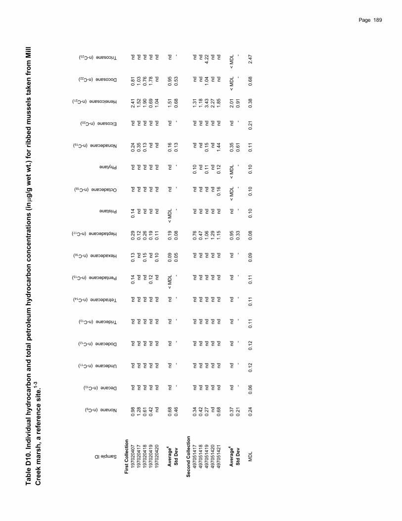
Tabl

e D

10. I

ndiv

idua

l hyd

roca

rbon

and

tota

l pet

role

um h

ydro

carb

on c

once

ntra

tions

(in

g/g

wet

wt.)

for r

ibbe

d m

usse

ls ta

ken

from

Mill

C

reek

mar

sh, a

refe

renc

e si

te.1-

3

Sample ID

Nonane (n-C9)

Decane (n-C10)

Undecane (n-C11)

Dodecane (n-C12)

Tridecane (n-C13)

Tetradecane (n-C14)

Pentadecane (n-C15)

Hexadecane (n-C16)

Heptadecane (n-C17)

Pristane

Octadecane (n-C18)

Phytane

Nonadecane (n-C19)

Eicosane (n-C20)

Heneicosane (n-C21)

Docosane (n-C22)

Tricosane (n-C23)

Firs

t Col

lect

ion

1970

2040

70.

98nd

ndnd

ndnd

0.14

0.13

0.29

0.14

ndnd

0.24

nd2.

410.

81nd

1970

2041

71.

28nd

ndnd

ndnd

ndnd

0.12

ndnd

nd0.

35nd

1.52

1.03

nd19

7020

418

0.61

ndnd

ndnd

ndnd

0.15

0.26

ndnd

nd0.

13nd

1.90

0.76

nd19

7020

419

0.42

ndnd

ndnd

nd0.

12nd

0.19

ndnd

ndnd

nd0.

691.

78nd

1970

2042

0nd

ndnd

ndnd

ndnd

0.10

0.11

ndnd

ndnd

nd1.

04nd

nd

Ave

rage

40.

68nd

ndnd

ndnd

< M

DL

0.09

0.19

< M

DL

ndnd

0.16

nd1.

510.

95nd

Std

Dev

0.46

--

--

--

0.05

0.08

--

-0.

13-

0.68

0.53

-

Seco

nd C

olle

ctio

n49

7051

417

0.34

ndnd

ndnd

ndnd

nd0.

76nd

nd0.

10nd

nd1.

31nd

nd49

7051

418

0.42

ndnd

ndnd

ndnd

nd0.

47nd

ndnd

ndnd

1.18

ndnd

4970

5141

90.

27nd

ndnd

ndnd

ndnd

1.06

ndnd

0.11

0.15

nd3.

431.

044.

2249

7051

420

ndnd

ndnd

ndnd

ndnd

1.29

ndnd

ndnd

nd2.

27nd

nd49

7051

421

0.68

ndnd

ndnd

ndnd

nd1.

15nd

0.16

0.12

1.44

nd1.

85nd

nd

Ave

rage

40.

37nd

ndnd

ndnd

ndnd

0.95

nd<

MD

L<

MD

L0.

35nd

2.01

< M

DL

< M

DL

Std

Dev

0.21

--

--

--

-0.

33-

--

0.61

-0.

91-

-

MD

L0.

240.

060.

120.

120.

110.

110.

110.

090.

080.

100.

100.

100.

110.

210.

380.

682.

47

189Page

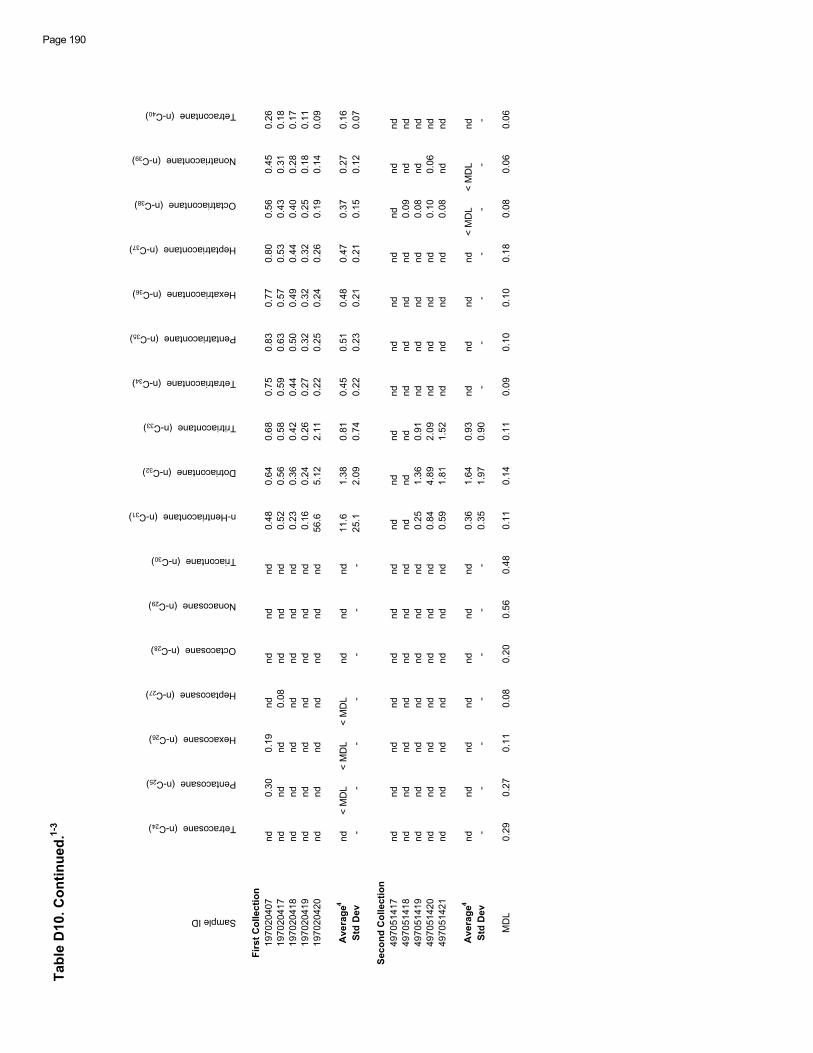
Tabl

e D

10. C

ontin

ued.

1-3

Sample ID

Tetracosane (n-C24)

Pentacosane (n-C25)

Hexacosane (n-C26)

Heptacosane (n-C27)

Octacosane (n-C28)

Nonacosane (n-C29)

Triacontane (n-C30)

n-Hentriacontane (n-C31)

Dotriacontane (n-C32)

Tritriacontane (n-C33)

Tetratriacontane (n-C34)

Pentatriacontane (n-C35)

Hexatriacontane (n-C36)

Heptatriacontane (n-C37)

Octatriacontane (n-C38)

Nonatriacontane (n-C39)

Tetracontane (n-C40)

Firs

t Col

lect

ion

1970

2040

7

nd

0.

30

0.

19

nd

nd

nd

nd

0.

48

0.

64

0.

68

0.

75

0.

83

0.

77

0.

80

0.

56

0.

45

0.

2619

7020

417

n

d

n

d

n

d

0.08

n

d

n

d

n

d

0.52

0.56

0.58

0.59

0.63

0.57

0.53

0.43

0.31

0.18

1970

2041

8

nd

nd

nd

nd

nd

nd

nd

0.

23

0.

36

0.

42

0.

44

0.

50

0.

49

0.

44

0.

40

0.

28

0.

1719

7020

419

n

d

n

d

n

d

n

d

n

d

n

d

n

d

0.16

0.24

0.26

0.27

0.32

0.32

0.32

0.25

0.18

0.11

1970

2042

0

nd

nd

nd

nd

nd

nd

nd

56.

6

5.

12

2.

11

0.

22

0.

25

0.

24

0.

26

0.

19

0.

14

0.

09

Ave

rage

4

nd

<

MD

L

< M

DL

<

MD

L

n

d

n

d

n

d

1

1.6

1.38

0.81

0.45

0.51

0.48

0.47

0.37

0.27

0.16

Std

Dev

-

-

-

-

-

-

-

2

5.1

2.09

0.74

0.22

0.23

0.21

0.21

0.15

0.12

0.07

Seco

nd C

olle

ctio

n49

7051

417

n

d

n

d

n

d

n

d

n

d

n

d

n

d

n

d

n

d

n

d

n

d

n

d

n

d

n

d

n

d

n

d

n

d

4970

5141

8

nd

nd

nd

nd

nd

nd

nd

nd

nd

nd

nd

nd

nd

nd

0.

09

nd

nd

49

7051

419

n

d

n

d

n

d

n

d

n

d

n

d

n

d

0.25

1.36

0.91

n

d

n

d

n

d

n

d

0.08

n

d

n

d

4970

5142

0

nd

nd

nd

nd

nd

nd

nd

0.

84

4.

89

2.

09

nd

nd

nd

nd

0.

10

0.

06

nd

49

7051

421

n

d

n

d

n

d

n

d

n

d

n

d

n

d

0.59

1.81

1.52

n

d

n

d

n

d

n

d

0.08

n

d

n

d

Ave

rage

4

nd

nd

nd

nd

nd

nd

nd

0.

36

1.

64

0.

93

nd

nd

nd

nd

<

MD

L

< M

DL

nd

St

d D

ev

-

-

-

-

-

-

-

0.

35

1.

97

0.

90

-

-

-

-

-

-

-

MD

L0.

290.

270.

110.

080.

200.

560.

480.

110.

140.

110.

090.

100.

100.

180.

080.

060.

06

Page 190

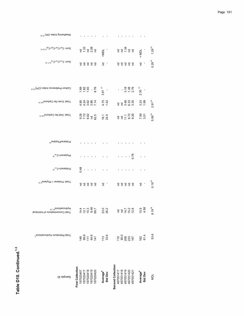
Tabl

e D

10. C

ontin

ued.

1-3

Sample ID

Total Petroleum Hydrocarbons5

Total Concentrations of Individual Hydrocarbons

6,7,15

Total: Pristane + Phytane6,15

Pristane/n-C1716

Phytane/n-C1816

Pristane/Phytane16

Total: Odd No Carbons6,8,15

Total: Even No Carbons6,9,15

Carbon Preference Index (CPI)10,16

Sum: C10-C12-C146,11,15

Sum: C22-C24-C26-C286,12,15

Weathering Index (WI)13,16

Firs

t Col

lect

ion

1970

2040

7

148

14.

4

nd

0.

48

-

-

9.

28

4.

90

1.

89

nd

nd

-

1970

2041

7

99.

9

12.

1

nd

-

-

-

7.

72

4.

24

1.

82

nd

1.

33

-

1970

2041

8

111

10.

3

nd

-

-

-

6.

62

3.

62

1.

83

nd

nd

-

1970

2041

9

64.

6

8.

46

nd

-

-

-

nd

3.

86

-

nd

2.

08

-

1970

2042

0

141

69.

7

nd

-

-

-

62.

5

7.

14

8.

76

nd

nd

-

Ave

rage

4

113

23.

0

nd

-

-

-

18.

1

4.

75

3.8

1 17

n

d

<M

DL

-

St

d D

ev

33.

6

26.

2

-

-

-

-

24.

9

1.

42

-

-

-

-

Seco

nd C

olle

ctio

n49

7051

417

1

10

n

d

n

d

-

-

-

n

d

n

d

-

n

d

n

d

- 49

7051

418

9

0.0

n

d

n

d

-

-

-

n

d

n

d

-

n

d

n

d

- 49

7051

419

2

08

1

4.7

n

d

-

-

-

1

1.1

3.48

3.18

n

d

1.34

- 49

7051

420

2

33

1

5.2

n

d

-

-

-

8.72

6.33

1.38

n

d

n

d

- 49

7051

421

1

67

1

2.8

n

d

-

0.78

-

9.26

3.35

2.76

n

d

n

d

-

Ave

rage

4

162

10.

9

nd

-

-

-

7.

59

3.

23

2.3

5 17

n

d

< M

DL

-

St

d D

ev

61.

4

4.

58

-

-

-

-

3.

01

1.

99

-

-

-

-

MD

L

53

.68.

1914

0.19

145.

0914

2.91

140.

2914

1.29

14

191Page

Tabl

e D

10. C

ontin

ued.

Foot

note

s:1

Th

e co

ncen

tratio

ns o

f the

indi

vidu

al a

lipha

tic h

ydro

carb

ons

and

the

tota

l pet

role

um h

ydro

carb

ons

wer

e de

term

ined

usi

ng e

xter

nal s

tand

ard

calc

ulat

ions

.2

W

hen

an in

divi

dual

alip

hatic

hyd

roca

rbon

was

not

det

ecte

d, it

s co

ncen

tratio

n w

as re

plac

ed b

y nd

.3

Th

e co

ncen

tratio

ns fo

r n-C

8 will

be

not r

epor

ted,

sin

ce it

was

diff

icul

t to

iden

tify

this

pea

k in

sam

ples

and

to d

eter

min

e M

DL

for n

-C8.

4

If al

l con

cent

ratio

ns a

re n

d, th

e av

erag

e is

repl

aced

with

nd.

Whe

n th

ere

is a

t lea

st o

ne n

umbe

r in

the

data

set

to b

e av

erag

ed, e

ach

nd is

repl

aced

w

ith 1

/2*M

DL,

and

an

aver

age

is c

alcu

late

d. If

this

num

eric

val

ue is

less

than

the

MD

L, th

e av

erag

e is

repl

aced

by

< M

DL;

oth

erw

ise,

the

aver

age

is th

eca

lcul

ated

val

ue. W

hen

a nu

mer

ic v

alue

is fo

und

for t

he a

vera

ge, t

he s

tand

ard

devi

atio

n is

then

det

erm

ined

usi

ng th

e sa

me

num

ber s

et u

sed

to c

alcu

late

the

aver

age.

5

D

eter

min

ed fr

om th

e to

tal p

eak

area

s in

the

chro

mat

ogra

m fr

om n

-C8 t

o n-

C40

min

us a

ny c

ontri

butio

ns fr

om th

e in

tern

al s

tand

ard

area

s.6

Th

ese

form

ulae

use

1/2

MD

L va

lues

for e

ach

anal

yte

not d

etec

ted.

7

Sum

of t

he c

once

ntra

tions

of t

he in

divi

dual

alip

hatic

hyd

roca

rbon

s n-

C9 t

hrou

gh n

-C40

plu

s th

e co

ncen

tratio

ns o

f pris

tane

and

phy

tane

.8

Th

e to

tal o

f the

con

cent

ratio

ns o

f the

alip

hatic

hyd

roca

rbon

s w

ith a

n od

d nu

mbe

r of c

arbo

n at

oms.

9

The

tota

l of t

he c

once

ntra

tions

of t

he a

lipha

tic h

ydro

carb

ons

with

an

even

num

ber o

f car

bon

atom

s. T

he c

ontri

butio

n of

n-C

8 is

not i

nclu

ded

in th

e to

tal.

10

Car

bon

Pre

fere

nce

Inde

x (C

PI)

is d

efin

ed a

s th

e ra

tio o

f the

tota

l of t

he c

once

ntra

tions

of t

he a

lipha

tic h

ydro

carb

ons

with

an

odd

num

ber o

f car

bons

to th

eto

tal c

once

ntra

tion

of th

e al

phat

ic h

ydro

carb

ons

with

an

even

car

bon

num

ber.

11Th

e to

tal o

f the

con

cent

ratio

ns o

f n-C

10, n

-C12

, and

n-C

14.

12 T

he to

tal o

f the

con

cent

ratio

ns o

f n-C

22, n

-C24

, n-C

26, a

nd n

-C28

.13

W

eath

erin

g In

dex

(WI)

is d

efin

ed a

s th

e ra

tio o

f the

tota

l con

cent

ratio

n of

n-C

10, n

-C12

, and

n-C

14 to

the

tota

l con

cent

ratio

n of

n-C

22, n

-C24

, n-C

26, a

nd n

-C28

.14

T

hese

MD

L va

lues

are

cal

cula

ted

with

the

sam

e su

mm

atio

n fo

rmul

ae a

s th

e sa

mpl

es u

sing

the

indi

vidu

al h

ydro

carb

on M

DL

valu

es.

15

The

sum

mat

ion

tota

ls fo

r the

sam

ples

are

com

pare

d w

ith c

alcu

late

d M

DL

valu

es o

btai

ned

usin

g th

e sa

me

sum

mat

ion

form

ulae

as

the

sam

ples

.W

hen

thes

e sa

mpl

e to

tals

wer

e le

ss th

an th

e to

tal M

DL,

its

valu

e w

as re

plac

ed b

y nd

. The

ave

rage

s an

d st

anda

rd d

evia

tions

for t

he to

tals

wer

etre

ated

in th

e sa

me

way

as

the

indi

vidu

al h

ydro

carb

ons;

see

foot

note

4.

16

Num

eric

al v

alue

s of

the

CP

I, W

I, an

d th

e ra

tios:

pris

tane

/n-C

17, p

hyta

ne/n

-C18

, and

pris

tane

/phy

tane

, will

be

calc

ulat

ed o

nly

whe

n th

e de

fined

qua

ntity

for e

ach

inde

x or

ratio

has

a n

umer

ic v

alue

.17

T

hese

resu

lts a

re n

ot tr

ue a

vera

ges,

inst

ead

they

are

the

ratio

s of

the

aver

ages

of t

he d

efin

ed q

uant

ities

, if t

hese

ave

rage

s ex

ist.

Page 192

Tabl

e D

11. I

ndiv

idua

l hyd

roca

rbon

and

tota

l pet

role

um h

ydro

carb

on c

once

ntra

tions

(in

g/g

wet

wt.)

for r

ibbe

d m

usse

ls ta

ken

from

San

dy

Hoo

k m

arsh

, a re

fere

nce

site

.1-3

Sample ID

Nonane (n-C9)

Decane (n-C10)

Undecane (n-C11)

Dodecane (n-C12)

Tridecane (n-C13)

Tetradecane (n-C14)

Pentadecane (n-C15)

Hexadecane (n-C16)

Heptadecane (n-C17)

Pristane

Octadecane (n-C18)

Phytane

Nonadecane (n-C19)

Eicosane (n-C20)

Heneicosane (n-C21)

Docosane (n-C22)

Tricosane (n-C23)

2970

3171

0nd

ndnd

ndnd

ndnd

nd0.

09nd

ndnd

0.47

nd0.

581.

303.

4229

7031

711

0.47

nd0.

13nd

ndnd

nd0.

100.

13nd

ndnd

0.60

nd1.

211.

27nd

2970

3171

20.

34nd

ndnd

ndnd

ndnd

0.09

ndnd

nd0.

31nd

0.52

0.68

nd29

7031

713

0.30

ndnd

ndnd

ndnd

nd0.

12nd

ndnd

ndnd

1.09

1.42

nd29

7031

714

0.31

ndnd

ndnd

ndnd

ndnd

ndnd

nd0.

24nd

0.93

0.95

nd29

7031

715

0.34

ndnd

ndnd

ndnd

nd0.

12nd

ndnd

0.39

nd1.

581.

04nd

2970

3171

60.

32nd

ndnd

ndnd

ndnd

0.12

ndnd

nd0.

48nd

0.89

0.72

nd

Ave

rage

40.

31nd

< M

DL

ndnd

ndnd

< M

DL

0.10

ndnd

nd0.

36nd

0.97

1.06

< M

DL

Std

Dev

0.10

--

--

--

-0.

03-

--

0.18

-0.

370.

29-

MD

L0.

240.

060.

120.

120.

110.

110.

110.

090.

080.

100.

100.

100.

110.

210.

380.

682.

47

193Page

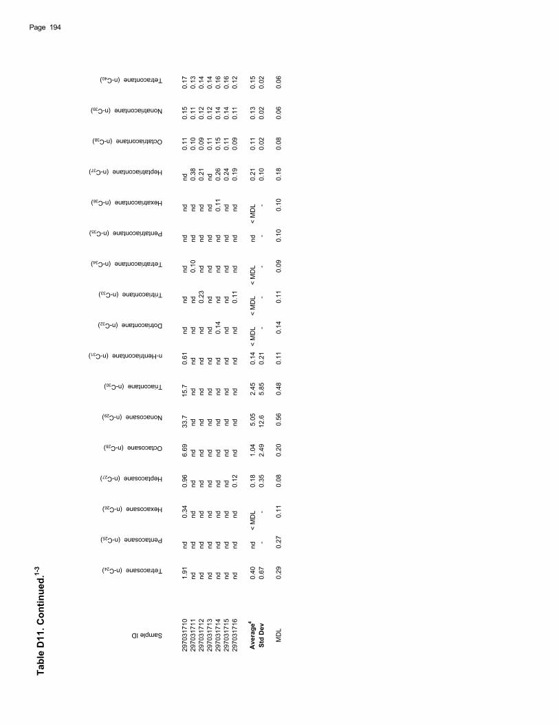
Tabl

e D

11. C

ontin

ued.

1-3

Sample ID

Tetracosane (n-C24)

Pentacosane (n-C25)

Hexacosane (n-C26)

Heptacosane (n-C27)

Octacosane (n-C28)

Nonacosane (n-C29)

Triacontane (n-C30)

n-Hentriacontane (n-C31)

Dotriacontane (n-C32)

Tritriacontane (n-C33)

Tetratriacontane (n-C34)

Pentatriacontane (n-C35)

Hexatriacontane (n-C36)

Heptatriacontane (n-C37)

Octatriacontane (n-C38)

Nonatriacontane (n-C39)

Tetracontane (n-C40)

2970

3171

0

1.

91

nd

0.

34

0.

96

6.

69

33.

7

15.

7

0.

61

nd

nd

nd

nd

nd

nd

0.

11

0.

15

0.

1729

7031

711

n

d

n

d

n

d

n

d

n

d

n

d

n

d

n

d

n

d

n

d

0.10

n

d

n

d

0.38

0.10

0.11

0.13

2970

3171

2

nd

nd

nd

nd

nd

nd

nd

nd

nd

0.

23

nd

nd

nd

0.

21

0.

09

0.

12

0.

1429

7031

713

n

d

n

d

n

d

n

d

n

d

n

d

n

d

n

d

n

d

n

d

n

d

n

d

n

d

n

d

0.11

0.12

0.14

2970

3171

4

nd

nd

nd

nd

nd

nd

nd

nd

0.

14

nd

nd

nd

0.

11

0.

26

0.

15

0.

14

0.

1629

7031

715

n

d

n

d

n

d

n

d

n

d

n

d

n

d

n

d

n

d

n

d

n

d

n

d

n

d

0.24

0.11

0.14

0.16

2970

3171

6

nd

nd

nd

0.

12

nd

nd

nd

nd

nd

0.

11

nd

nd

nd

0.

19

0.

09

0.

11

0.

12

Ave

rage

4

0.

40

nd

<

MD

L

0.18

1.04

5.05

2.45

0.14

< M

DL

<

MD

L

< M

DL

nd

<

MD

L

0.21

0.11

0.13

0.15

Std

Dev

0.67

-

-

0.35

2.49

1

2.6

5.85

0.21

-

-

-

-

-

0.10

0.02

0.02

0.02

MD

L0.

290.

270.

110.

080.

200.

560.

480.

110.

140.

110.

090.

100.

100.

180.

080.

060.

06

Page 194

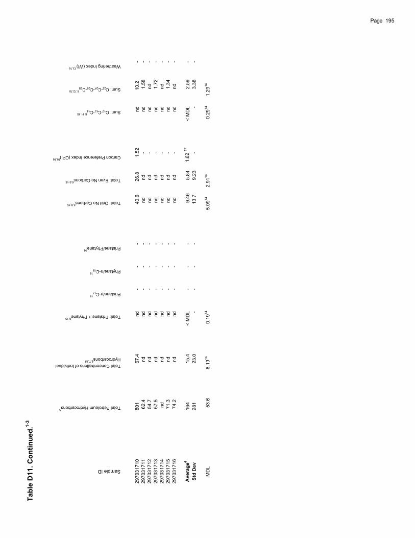
Tabl

e D

11. C

ontin

ued.

1-3

Sample ID

Total Petroleum Hydrocarbons5

Total Concentrations of Individual Hydrocarbons

6,7,15

Total: Pristane + Phytane6,15

Pristane/n-C1716

Phytane/n-C1816

Pristane/Phytane16

Total: Odd No Carbons6,8,15

Total: Even No Carbons6,9,15

Carbon Preference Index (CPI)10,16

Sum: C10-C12-C146,11,15

Sum: C22-C24-C26-C286,12,15

Weathering Index (WI)13,16

2970

3171

0

801

67.

4

nd

-

-

-

40.

6

26.

8

1.

52

nd

10.

2

-

2970

3171

1

62.

4

nd

nd

-

-

-

nd

nd

-

nd

1.

58

-

2970

3171

2

54.

7

nd

nd

-

-

-

nd

nd

-

nd

nd

-

2970

3171

3

57.

5

nd

nd

-

-

-

nd

nd

-

nd

1.

72

-

2970

3171

4

nd

nd

nd

-

-

-

nd

nd

-

nd

nd

-

2970

3171

5

71.

3

nd

nd

-

-

-

nd

nd

-

nd

1.

34

-

2970

3171

6

74.

2

nd

nd

-

-

-

nd

nd

-

nd

nd

-

Ave

rage

4

164

15.

4

< M

DL

-

-

-

9.

46

5.

84

1.6

2 17

<

MD

L

2.59

-

Std

Dev

2

81

2

3.0

-

-

-

-

1

3.7

9.23

-

-

3.38

-

MD

L

53

.68.

1914

0.19

145.

0914

2.91

140.

2914

1.29

14

195Page

Tabl

e D

11. C

ontin

ued.

Foot

note

s:1

Th

e co

ncen

tratio

ns o

f the

indi

vidu

al a

lipha

tic h

ydro

carb

ons

and

the

tota

l pet

role

um h

ydro

carb

ons

wer

e de

term

ined

usi

ng e

xter

nal s

tand

ard

calc

ulat

ions

.2

W

hen

an in

divi

dual

alip

hatic

hyd

roca

rbon

was

not

det

ecte

d, it

s co

ncen

tratio

n w

as re

plac

ed b

y nd

.3

Th

e co

ncen

tratio

ns fo

r n-C

8 will

be

not r

epor

ted,

sin

ce it

was

diff

icul

t to

iden

tify

this

pea

k in

sam

ples

and

to d

eter

min

e M

DL

for n

-C8.

4

If al

l con

cent

ratio

ns a

re n

d, th

e av

erag

e is

repl

aced

with

nd.

Whe

n th

ere

is a

t lea

st o

ne n

umbe

r in

the

data

set

to b

e av

erag

ed, e

ach

nd is

repl

aced

w

ith 1

/2*M

DL,

and

an

aver

age

is c

alcu

late

d. If

this

num

eric

val

ue is

less

than

the

MD

L, th

e av

erag

e is

repl

aced

by

< M

DL;

oth

erw

ise,

the

aver

age

is th

eca

lcul

ated

val

ue. W

hen

a nu

mer

ic v

alue

is fo

und

for t

he a

vera

ge, t

he s

tand

ard

devi

atio

n is

then

det

erm

ined

usi

ng th

e sa

me

num

ber s

et u

sed

to c

alcu

late

the

aver

age.

5

D

eter

min

ed fr

om th

e to

tal p

eak

area

s in

the

chro

mat

ogra

m fr

om n

-C8 t

o n-

C40

min

us a

ny c

ontri

butio

ns fr

om th

e in

tern

al s

tand

ard

area

s.6

Th

ese

form

ulae

use

1/2

MD

L va

lues

for e

ach

anal

yte

not d

etec

ted.

7

Sum

of t

he c

once

ntra

tions

of t

he in

divi

dual

alip

hatic

hyd

roca

rbon

s n-

C9 t

hrou

gh n

-C40

plu

s th

e co

ncen

tratio

ns o

f pris

tane

and

phy

tane

.8

Th

e to

tal o

f the

con

cent

ratio

ns o

f the

alip

hatic

hyd

roca

rbon

s w

ith a

n od

d nu

mbe

r of c

arbo

n at

oms.

9

The

tota

l of t

he c

once

ntra

tions

of t

he a

lipha

tic h

ydro

carb

ons

with

an

even

num

ber o

f car

bon

atom

s. T

he c

ontri

butio

n of

n-C

8 is

not i

nclu

ded

in th

e to

tal.

10

Car

bon

Pre

fere

nce

Inde

x (C

PI)

is d

efin

ed a

s th

e ra

tio o

f the

tota

l of t

he c

once

ntra

tions

of t

he a

lipha

tic h

ydro

carb

ons

with

an

odd

num

ber o

f car

bons

to th

eto

tal c

once

ntra

tion

of th

e al

phat

ic h

ydro

carb

ons

with

an

even

car

bon

num

ber.

11Th

e to

tal o

f the

con

cent

ratio

ns o

f n-C

10, n

-C12

, and

n-C

14.

12 T

he to

tal o

f the

con

cent

ratio

ns o

f n-C

22, n

-C24

, n-C

26, a

nd n

-C28

.13

W

eath

erin

g In

dex

(WI)

is d

efin

ed a

s th

e ra

tio o

f the

tota

l con

cent

ratio

n of

n-C

10, n

-C12

, and

n-C

14 to

the

tota

l con

cent

ratio

n of

n-C

22, n

-C24

, n-C

26, a

nd n

-C28

.14

T

hese

MD

L va

lues

are

cal

cula

ted

with

the

sam

e su

mm

atio

n fo

rmul

ae a

s th

e sa

mpl

es u

sing

the

indi

vidu

al h

ydro

carb

on M

DL

valu

es.

15

The

sum

mat

ion

tota

ls fo

r the

sam

ples

are

com

pare

d w

ith c

alcu

late

d M

DL

valu

es o

btai

ned

usin

g th

e sa

me

sum

mat

ion

form

ulae

as

the

sam

ples

.W

hen

thes

e sa

mpl

e to

tals

wer

e le

ss th

an th

e to

tal M

DL,

its

tota

l was

repl

aced

by

nd. T

he a

vera

ges

and

stan

dard

dev

iatio

ns fo

r the

tota

ls w

ere

treat

ed in

the

sam

e w

ay a

s th

e in

divi

dual

hyd

roca

rbon

s; s

ee fo

otno

te 4

.16

N

umer

ical

val

ues

of th

e C

PI,

WI,

and

the

ratio

s: p

rista

ne/n

-C17

, phy

tane

/n-C

18, a

nd p

rista

ne/p

hyta

ne, w

ill b

e ca

lcul

ated

onl

y w

hen

the

defin

ed q

uant

ityfo

r eac

h in

dex

or ra

tio h

as a

num

eric

val

ue.

17

The

se re

sults

are

not

true

ave

rage

s, in

stea

d th

ey a

re th

e ra

tios

of th

e av

erag

es o

f the

def

ined

qua

ntiti

es, i

f the

se a

vera

ges

exis

t.

Page 196

Page 197

APPENDIX E

CHROMATOGRAMS FOR ANALYSIS OF PETROLEUM HYDROCARBONS

[Note: For Figures E1-E14, each chromatogram was normalized to the overall response expected for1 g of material from each core section or surface scoop sample. The value for TPH is given for eachchromatogram. When the TPH value is smaller than the MDL value of 181μg/g, the symbol “<MDL” isassigned to the TPH concentration, and the MDL is used to normalize the chromatogram.]

Figure E1. Normalized GC-FID chromatograms for Station A, Old Place Creek marsh sediment core sections (collectedSeptember 1996) and surface scoop (collected May 1997)

Figure E2. Normalized GC-FID chromatograms for Station B, Old Place Creek marsh sediment core sections (collectedSeptember 1996) and surface scoop (collected May 1997)

Figure E3. Normalized GC-FID chromatograms for Station C, Old Place Creek marsh sediment core sections (collectedSeptember 1996) and surface scoop (collected May 1997)

Figure E4. Normalized GC-FID chromatograms for Station D, Old Place Creek marsh sediment core sections (collectedSeptember 1996) and surface scoop (collected May 1997)

Figure E5. Normalized GC-FID chromatograms for Station A, Con Ed Tower marsh sediment core sections (collectedSeptember 1996) and surface scoop (collected May 1997)

Figure E6. Normalized GC-FID chromatograms for Station B, Con Ed Tower marsh sediment core sections (collectedSeptember 1996) and surface scoop (collected May 1997)

Figure E7. Normalized GC-FID chromatograms for Station C, Con Ed Tower marsh sediment core sections (collectedSeptember 1996) and surface scoop (collected May 1997)

Figure E8. Normalized GC-FID chromatograms for Station D, Con Ed Tower marsh sediment core sections (collectedSeptember 1996) and surface scoop (collected May 1997)

Figure E9. Normalized GC-FID chromatograms for Station A, Mill Creek marsh sediment core sections (collectedSeptember 1996)

Figure E10. Normalized GC-FID chromatograms for Station B, Mill Creek marsh sediment core sections (collectedSeptember 1996)

Figure E11. Normalized GC-FID chromatograms for Station C, Mill Creek marsh sediment core sections (collectedSeptember 1996)

Figure E12. Normalized GC-FID chromatograms for Station D, Mill Creek marsh sediment core sections (collectedSeptember 1996)

Figure E13. Normalized GC-FID chromatograms for Old Place Creek marsh and Sandy Hook Bay marsh surface scoopsamples

Figure E14. Normalized GC-FID chromatograms for Con Ed Tower marsh and Sandy Hook Bay marsh surface scoopsamples

Figure E15. Representative GC-FID chromatograms for Arthur Kill and Sandy Hook Bay ribbed-mussels collected inSeptember 1996

Figure E16. Representative GC-FID chromatograms for Arthur Kill ribbed-mussels collected in May 1997

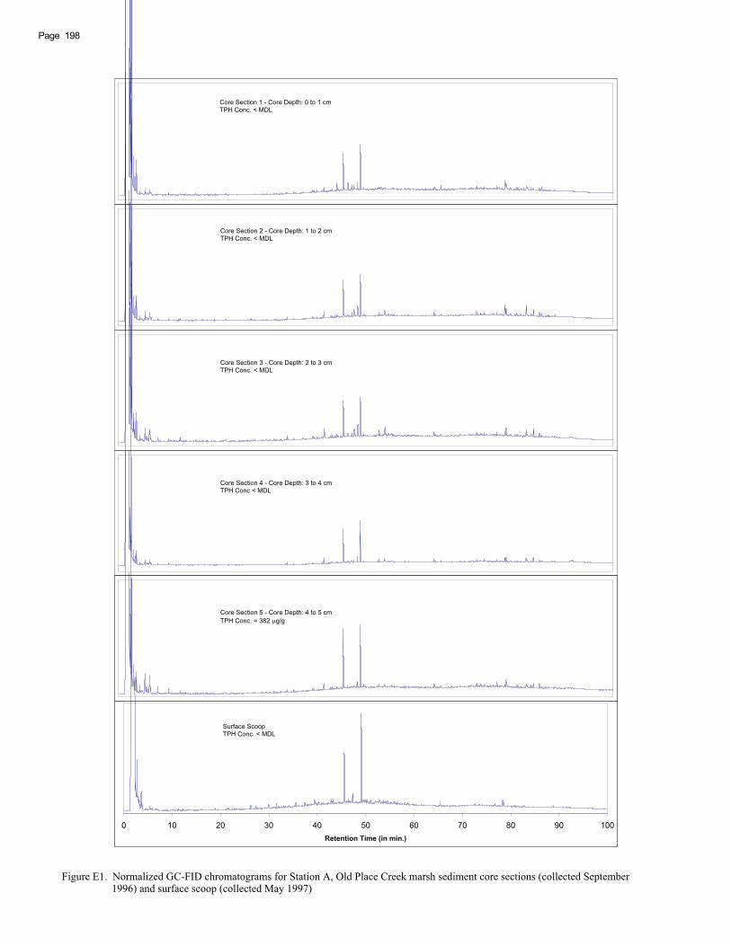
Core Section 4 - Core Depth: 3 to 4 cmTPH Conc < MDL

Core Section 3 - Core Depth: 2 to 3 cmTPH Conc. < MDL

Core Section 5 - Core Depth: 4 to 5 cmTPH Conc. = 382 g/g

0 10 20 30 40 50 60 70 80 90 100Retention Time (in min.)

Surface ScoopTPH Conc. < MDL

Core Section 1 - Core Depth: 0 to 1 cmTPH Conc. < MDL

Core Section 2 - Core Depth: 1 to 2 cmTPH Conc. < MDL

Page 198

Figure E1. Normalized GC-FID chromatograms for Station A, Old Place Creek marsh sediment core sections (collected September 1996) and surface scoop (collected May 1997)

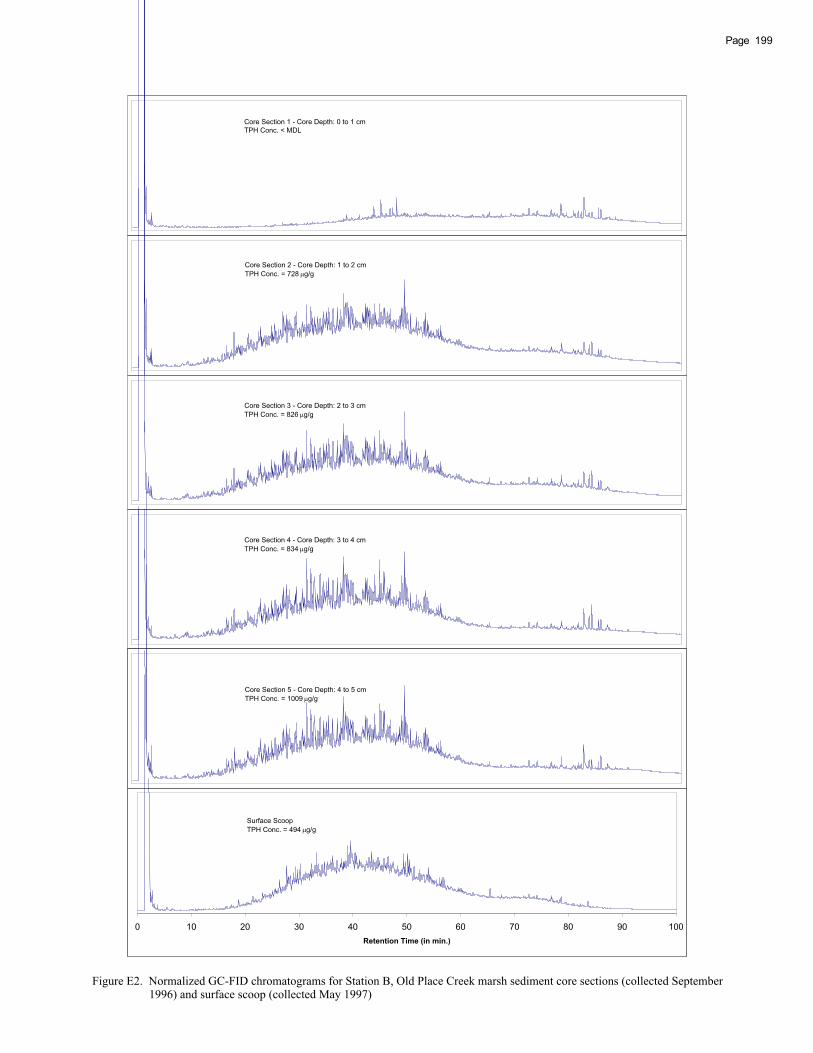
Core Section 4 - Core Depth: 3 to 4 cmTPH Conc. = 834 g/g

Core Section 3 - Core Depth: 2 to 3 cmTPH Conc. = 826 g/g

Core Section 5 - Core Depth: 4 to 5 cmTPH Conc. = 1009 g/g

0 10 20 30 40 50 60 70 80 90 100Retention Time (in min.)

Surface ScoopTPH Conc. = 494 g/g

Core Section 1 - Core Depth: 0 to 1 cmTPH Conc. < MDL

Core Section 2 - Core Depth: 1 to 2 cmTPH Conc. = 728 g/g

199Page

Figure E2. Normalized GC-FID chromatograms for Station B, Old Place Creek marsh sediment core sections (collected September 1996) and surface scoop (collected May 1997)

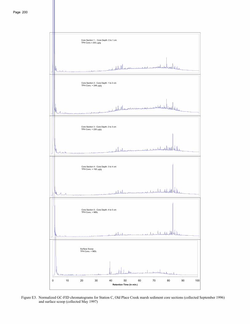
Core Section 4 - Core Depth: 3 to 4 cmTPH Conc. = 192 g/g

Core Section 3 - Core Depth: 2 to 3 cmTPH Conc. = 230 g/g

Core Section 5 - Core Depth: 4 to 5 cmTPH Conc. < MDL

0 10 20 30 40 50 60 70 80 90 100Retention Time (in min.)

Surface ScoopTPH Conc. < MDL

Core Section 1 - Core Depth: 0 to 1 cmTPH Conc.= 203 g/g

Core Section 2 - Core Depth: 1 to 2 cmTPH Conc. = 248 g/g

Page 200

Figure E3. Normalized GC-FID chromatograms for Station C, Old Place Creek marsh sediment core sections (collected September 1996) and surface scoop (collected May 1997)

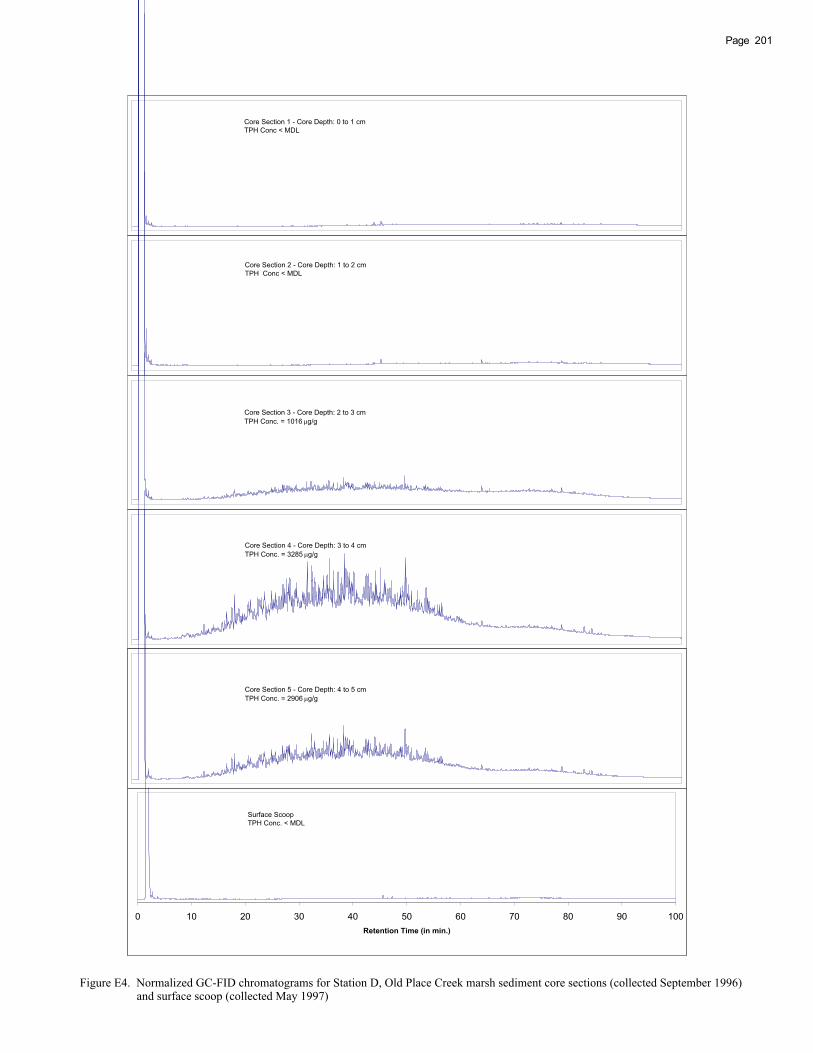
Core Section 4 - Core Depth: 3 to 4 cmTPH Conc. = 3285 g/g

Core Section 3 - Core Depth: 2 to 3 cmTPH Conc. = 1016 g/g

Core Section 5 - Core Depth: 4 to 5 cmTPH Conc. = 2906 g/g

0 10 20 30 40 50 60 70 80 90 100Retention Time (in min.)

Surface ScoopTPH Conc. < MDL

Core Section 1 - Core Depth: 0 to 1 cmTPH Conc < MDL

Core Section 2 - Core Depth: 1 to 2 cmTPH Conc < MDL

201Page

Figure E4. Normalized GC-FID chromatograms for Station D, Old Place Creek marsh sediment core sections (collected September 1996) and surface scoop (collected May 1997)

Core Section 4 - Core Depth: 3 to 4 cmTPH Conc. = 10068 g/g

Core Section 3 - Core Depth: 2 to 3 cmTPH Conc. 5273 g/g

Core Section 5 - Core Depth: 4 to 5 cmTPH Conc. = 12900 g/g

0 10 20 30 40 50 60 70 80 90 100

Retention Time (in min.)

Surface ScoopTPH Conc. = 1098 g/g

Core Section 1 - Core Depth: 0 to 1 cmTPH Conc. = 1363 g/g

Core Section 2 - Core Depth: 1 to 2 cmTPH Conc.= 4914 g/g

Page 202

Figure E5. Normalized GC-FID chromatograms for Station A, Con Ed Tower marsh sediment core sections (collected September 1996) and surface scoop (collected May 1997)

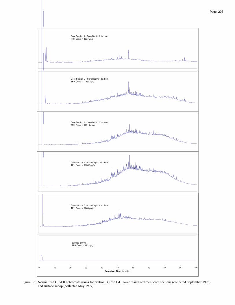
Core Section 4 - Core Depth: 3 to 4 cmTPH Conc. = 17300 g/g

Core Section 3 - Core Depth: 2 to 3 cmTPH Conc. = 12910 g/g

Core Section 5 - Core Depth: 4 to 5 cmTPH Conc. = 9060 g/g

0 10 20 30 40 50 60 70 80 90 100

Retention Time (in min.)

Surface ScoopTPH Conc. = 193 g/g

Core Section 1 - Core Depth: 0 to 1 cmTPH Conc. = 3837 g/g

Core Section 2 - Core Depth: 1 to 2 cmTPH Conc.= 11950 g/g

203Page

Figure E6. Normalized GC-FID chromatograms for Station B, Con Ed Tower marsh sediment core sections (collected September 1996) and surface scoop (collected May 1997)

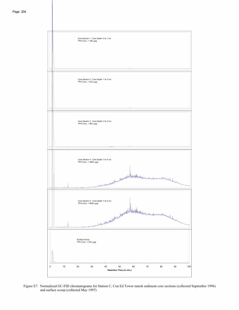
Core Section 4 - Core Depth: 3 to 4 cmTPH Conc. = 5660 g/g

Core Section 3 - Core Depth: 2 to 3 cmTPH Conc. = 852 g/g

Core Section 5 - Core Depth: 4 to 5 cmTPH Conc. = 8830 g/g

0 10 20 30 40 50 60 70 80 90 100Retention Time (in min.)

Surface ScoopTPH Conc. = 225 g/g

Core Section 1 - Core Depth: 0 to 1 cmTPH Conc. = 198 g/g

Core Section 2 - Core Depth: 1 to 2 cmTPH Conc. = 233 g/g

Page 204

Figure E7. Normalized GC-FID chromatograms for Station C, Con Ed Tower marsh sediment core sections (collected September 1996) and surface scoop (collected May 1997)

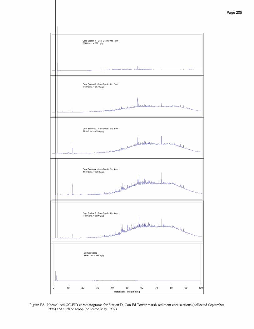
Core Section 4 - Core Depth: 3 to 4 cmTPH Conc. = 7260 g/g

Core Section 3 - Core Depth: 2 to 3 cmTPH Conc. = 4790 g/g

Core Section 5 - Core Depth: 4 to 5 cmTPH Conc. = 8500 g/g

0 10 20 30 40 50 60 70 80 90 100Retention Time (in min.)

Surface ScoopTPH Conc.= 357 g/g

Core Section 1 - Core Depth: 0 to 1 cmTPH Conc. = 677 g/g

Core Section 2 - Core Depth: 1 to 2 cmTPH Conc. = 3670 g/g

Page 205

Figure E8. Normalized GC-FID chromatograms for Station D, Con Ed Tower marsh sediment core sections (collected September 1996) and surface scoop (collected May 1997)

Core Section 3 - Core Depth: 2 to 3 cmTPH Conc. < MDL

Core Section 1 - Core Depth: 0 to 1 cmTPH Conc. < MDL

Core Section 2 - Core Depth: 1 to 2 cmTPH Conc. < MDL

0 10 20 30 40 50 60 70 80 90 100

Retention Time (in min.)

Core Section 4 - Core Depth: 3 to 4 cmTPH Conc. < MDL

Page 206

Figure E9. Normalized GC-FID chromatograms for Station A, Mill Creek marsh sediment core sections (collected September 1996)

Core Section 4 - Core Depth: 3 to 4 cmTPH Conc. < MDL

Core Section 3 - Core Depth: 2 to 3 cmTPH Conc. < MDL

0 10 20 30 40 50 60 70 80 90 100Retention Time (in min.)

Core Section 5 - Core Depth: 4 to 5 cmTPH Conc. < MDL

Core Section 1 - Core Depth: 0 to 1 cmTPH Conc. < MDL

Core Section 2 - Core Depth: 1 to 2 cmTPH Conc. < MDL

Page 207

Figure E10. Normalized GC-FID chromatograms for Station B, Mill Creek marsh sediment core sections (collected September 1996)

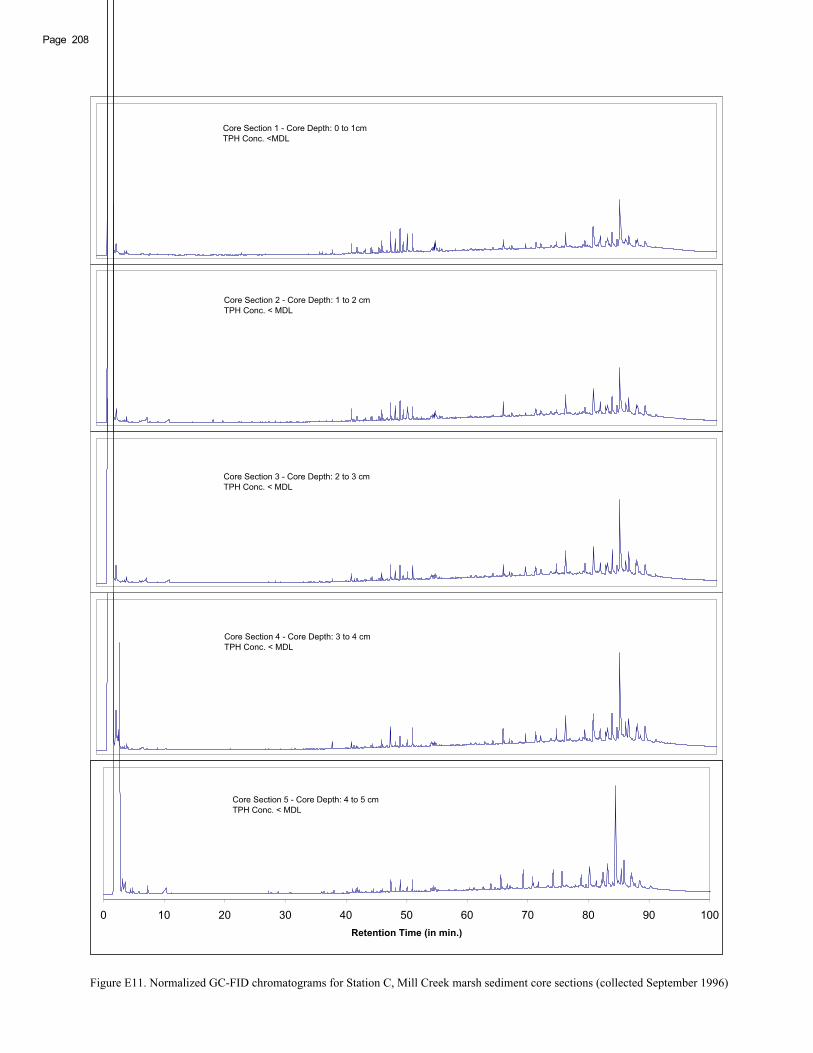
Core Section 4 - Core Depth: 3 to 4 cmTPH Conc. < MDL

Core Section 3 - Core Depth: 2 to 3 cmTPH Conc. < MDL

0 10 20 30 40 50 60 70 80 90 100Retention Time (in min.)

Core Section 5 - Core Depth: 4 to 5 cmTPH Conc. < MDL

Core Section 1 - Core Depth: 0 to 1cmTPH Conc. <MDL

Core Section 2 - Core Depth: 1 to 2 cmTPH Conc. < MDL

Page 208

Figure E11. Normalized GC-FID chromatograms for Station C, Mill Creek marsh sediment core sections (collected September 1996)

Core Section 4 - Core Depth: 3 to 4 cmTPH Conc. = 1665 g/g

Core Section 3 - Core Depth: 2 to 3 cmTPH Conc. = 1893 g/g

0 10 20 30 40 50 60 70 80 90 100Retention Time (in min.)

Core Section 5 - Core Depth: 4 to 5 cmTPH Conc. = 1400 g/g

Core Section 1 - Core Depth: 0 to 1 cmTPH Conc. < MDL

Core Section 2 - Core Depth: 1 to 2 cmTPH Conc. = 228 g/g

Page 209

Figure E12. Normalized GC-FID chromatograms for Station D, Mill Creek marsh sediment core sections (collected September 1996)

1 Each chromatogram was normalized with respect to the overall response expected for 1 gram of each surface scoop sample. The value for TPH is given for each chromatogram.

2 The TPH value for these samples is smaller than the MDL value of 181 g/g. The MDL value is used instead to normalize the chromatogram.

Old Place - Station C 2

TPH Conc. <MDL

Old Place - Station A 2

TPH Conc. <MDL

Old Place - Station B TPH Conc. = 494 g/g

Old Place - Station D 2

TPH Conc. <MDL

0 10 20 30 40 50 60 70 80 90 100Retention Time (in min.)

Sandy Hook 2

Page 210

Figure E13. Normalized GC-FID chromatograms for Old Place Creek marsh and Sandy Hook Bay marsh surface scoop samples1

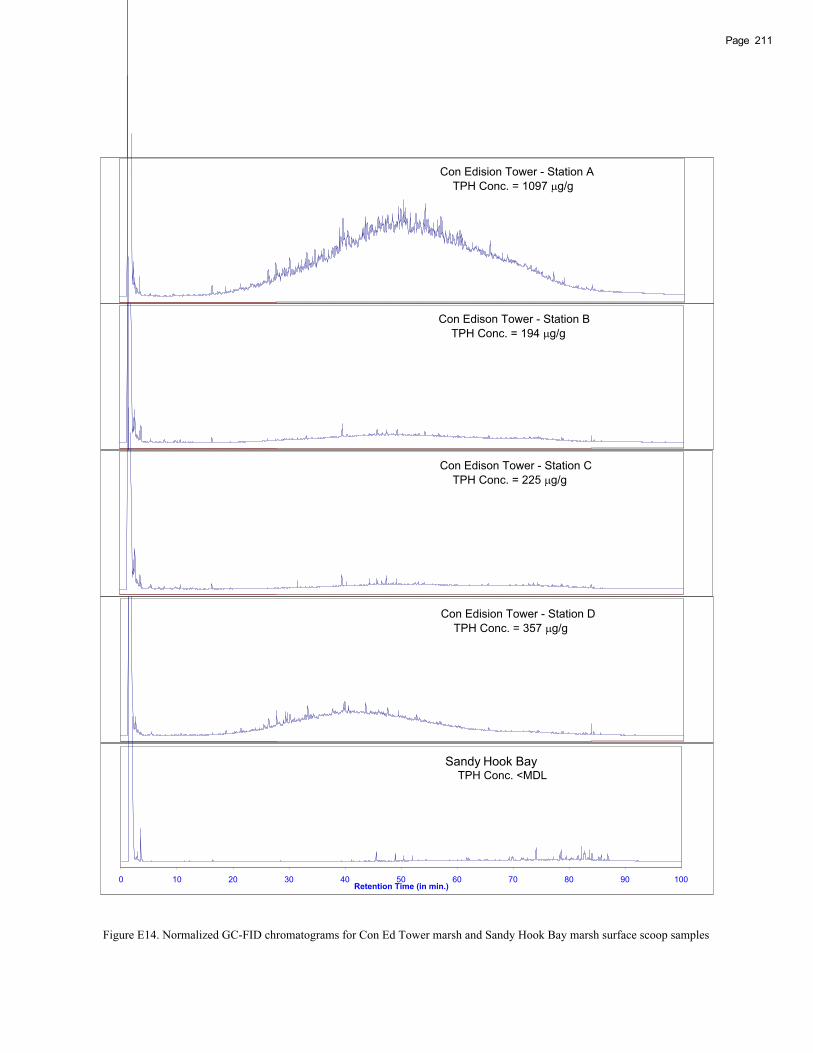
Con Edison Tower - Station B TPH Conc. = 194 g/g

Con Edision Tower - Station A TPH Conc. = 1097 g/g

Con Edision Tower - Station D TPH Conc. = 357 g/g

0 10 20 30 40 50 60 70 80 90 100Retention Time (in min.)

Sandy Hook Bay TPH Conc. <MDL

Con Edison Tower - Station C TPH Conc. = 225 g/g

211Page

Figure E14. Normalized GC-FID chromatograms for Con Ed Tower marsh and Sandy Hook Bay marsh surface scoop samples

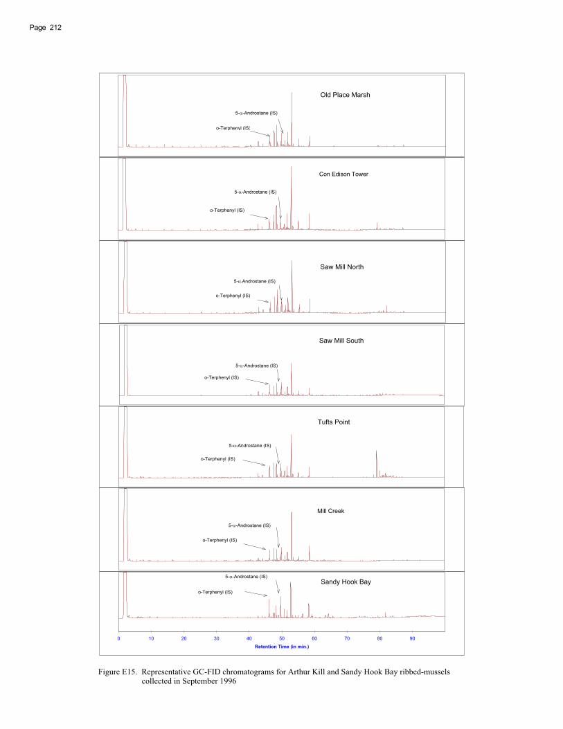
Tufts Point

5- -Androstane (IS)

o-Terphenyl (IS)

Mill Creek

5- -Androstane (IS)

o-Terphenyl (IS)

5- -Androstane (IS)

o-Terphenyl (IS)

Con Edison Tower

Saw Mill South

5- -Androstane (IS)

o-Terphenyl (IS)

0 10 20 30 40 50 60 70 80 90

Retention Time (in min.)

Sandy Hook Bay 5- -Androstane (IS)

o-Terphenyl (IS)

Old Place Marsh

5- -Androstane (IS)

o-Terphenyl (IS)

5- -Androstane (IS)

o-Terphenyl (IS)

Saw Mill North

Page 212

Figure E15. Representative GC-FID chromatograms for Arthur Kill and Sandy Hook Bay ribbed-mussels collected in September 1996

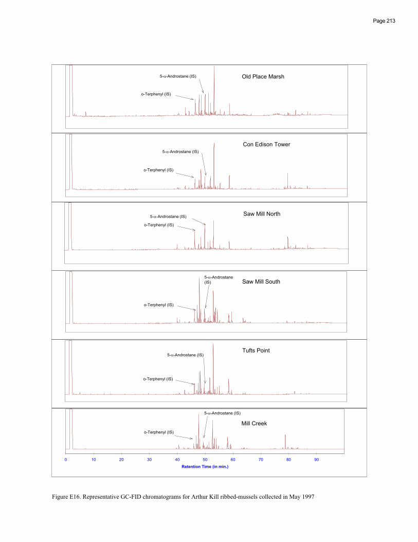
Saw Mill South 5- -Androstane(IS)

o-Terphenyl (IS)

Saw Mill North 5- -Androstane (IS)

o-Terphenyl (IS)

5- -Androstane (IS)

o-Terphenyl (IS)

0 10 20 30 40 50 60 70 80 90

Retention Time (in min.)

Mill Creek

5- -Androstane (IS)

o-Terphenyl (IS)

Con Edison Tower 5- -Androstane (IS)

o-Terphenyl (IS)

Tufts Point 5- -Androstane (IS)

o-Terphenyl (IS)

Old Place Marsh

Page 213

Figure E16. Representative GC-FID chromatograms for Arthur Kill ribbed-mussels collected in May 1997

Page 214

215Page

APPENDIX F

REDOX VALUES

Table F1. Summary of redox data by station, depth range, and season for the replanted marsh sites of Old Place Creekand Saw Mill Creek North

Table F2. Summary of redox data by station, depth range, and season for the unplanted marsh sites of Con Ed Towerand Saw Mill Creek South

Table F3. Summary of redox data by station, depth range, and season for the reference marsh sites of Tufts Point andMill Creek

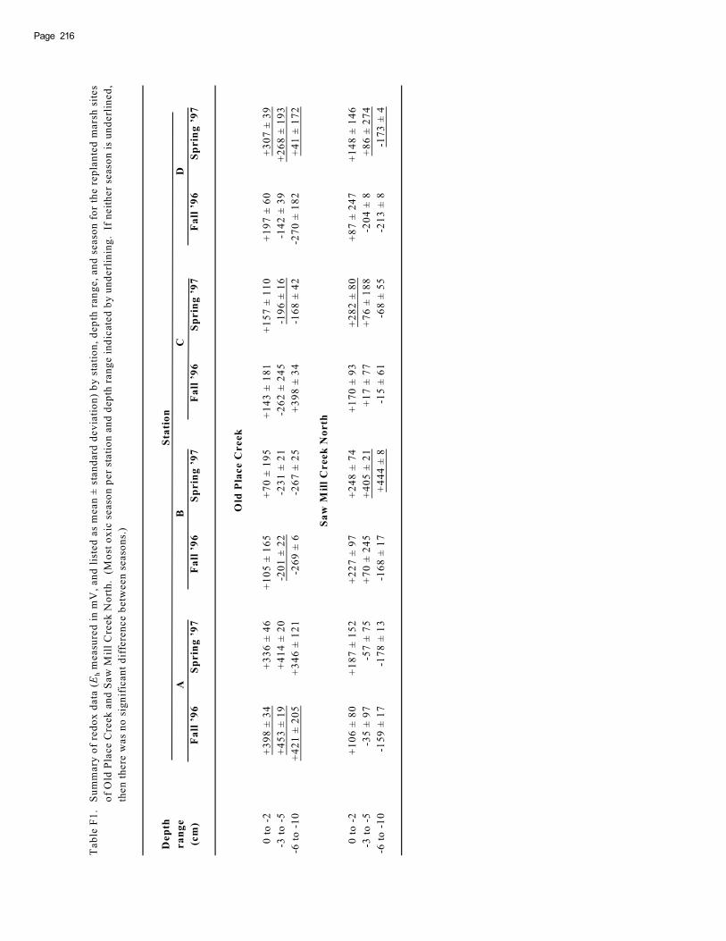
hT

ab

leF

1.

Su

mm

ary

of

red

ox

data

(E

measu

red

in m

V,

an

d l

iste

das

mean

± s

tan

dard

dev

iati

on

) b

y s

tati

on

, d

ep

thra

ng

e,

an

d s

easo

n f

or

the r

ep

lan

ted

mars

h s

ites

of

Old

Pla

ce

Cre

ek

an

d S

aw

Mil

l C

reek

No

rth

.(M

ost

ox

ic s

easo

n p

er

sta

tio

n a

nd

dep

th r

an

ge

ind

icate

db

y u

nd

erl

inin

g.

If

ne

ith

er

seaso

n i

s u

nd

erl

ine

d,

the

n t

here

was

no

sig

nif

ican

t d

iffe

ren

ce b

etw

een

seaso

ns.

)

De

pth

Sta

tio

n

ra

ng

eA

BC

D

(cm

)F

all

’9

6S

prin

g ’

97

Fa

ll ’

96

Sp

rin

g ’

97

Fa

ll ’

96

Sp

rin

g ’

97

Fa

ll ’

96

Sp

rin

g ’

97

Old

Pla

ce C

reek

0 t

o -

2+

39

8 ±

34

+3

36

± 4

6+

10

5 ±

16

5+

70

± 1

95

+1

43

± 1

81

+1

57

± 1

10

+1

97

± 6

0+

30

7 ±

39

-3 t

o -

5+

45

3 ±

19

+4

14

± 2

0-2

01

± 2

2-2

31

± 2

1-2

62

± 2

45

-19

6 ±

16

-14

2 ±

39

+2

68

± 1

93

-6 t

o -

10

+4

21

± 2

05

+3

46

± 1

21

-26

9 ±

6-2

67

± 2

5+

39

8 ±

34

-16

8 ±

42

-27

0 ±

18

2+

41

± 1

72

Sa

w M

ill

Creek

No

rth

0 t

o -

2+

10

6 ±

80

+1

87

± 1

52

+2

27

± 9

7+

24

8 ±

74

+1

70

± 9

3+

28

2 ±

80

+8

7 ±

24

7+

14

8 ±

14

6

-3 t

o -

5-3

5 ±

97

-57

± 7

5+

70

± 2

45

+4

05

± 2

1+

17

± 7

7+

76

± 1

88

-20

4 ±

8+

86

± 2

74

-6 t

o -

10

-15

9 ±

17

-17

8 ±

13

-16

8 ±

17

+4

44

± 8

-15

± 6

1-6

8 ±

55

-21

3 ±

8-1

73

± 4

Page 216

hT

ab

le F

2.

Su

mm

ary

of

red

ox

data

(E

measu

red

in m

V,

an

d l

iste

das

mean

± s

tan

dard

dev

iati

on

) b

y s

tati

on

, d

ep

th r

an

ge,

an

d s

easo

n f

or

the

un

pla

nte

d m

ars

h s

ites

of

Co

nE

d T

ow

er

an

dS

aw

Mil

lC

reek

So

uth

.(M

ost

ox

icse

aso

np

er

sta

tio

na

nd

de

pth

ran

ge

ind

icate

db

yu

nd

erl

inin

g.

Ifn

eit

he

rse

aso

n i

su

nd

erl

ine

d,

the

n t

here

was

no

sig

nif

ican

t d

iffe

ren

ce b

etw

een

seaso

ns.

)

De

pth

Sta

tio

n

ra

ng

eA

BC

D

(cm

)F

all

’9

6S

prin

g ’

97

Fa

ll ’

96

Sp

rin

g ’

97

Fa

ll ’

96

Sp

rin

g ’

97

Fa

ll ’

96

Sp

rin

g ’

97

Co

n E

d T

ow

er

0 t

o -

2+

59

± 1

61

+1

69

± 9

9+

23

± 1

23

+1

67

± 1

04

+1

09

± 4

4+

83

± 1

13

+8

± 1

13

+2

30

± 7

4

-3 t

o -

5-2

06

± 2

8+

52

± 2

38

-18

4 ±

38

-13

9 ±

17

7+

56

± 1

15

-11

8 ±

89

-15

6 ±

18

+1

43

± 2

80

-6 t

o -

10

-23

9 ±

10

+2

23

± 2

4-2

52

± 9

-20

6 ±

32

-13

4 ±

9-2

32

± 8

-17

0 ±

21

-97

± 2

12

Sa

w M

ill

Creek

So

uth

0 t

o -

2+

11

3 ±

14

9+

10

3 ±

15

4+

16

1 ±

13

6+

13

3 ±

14

6+

18

8 ±

12

3+

14

4 ±

11

0+

10

9 ±

13

3+

10

3 ±

13

0

-3 t

o -

5-1

51

± 1

5-1

79

± 1

8-1

29

± 4

0-1

40

± 2

4-5

8 ±

65

-18

± 3

6-1

76

± 1

2+

32

± 1

48

-6 t

o -

10

-19

1 ±

18

-18

4 ±

6-2

01

± 1

4-1

98

± 3

3-6

± 1

11

-12

9 ±

36

-20

5 ±

8+

61

± 9

8

Page 217

hT

ab

leF

3.

Su

mm

ary

of

red

ox

data

(E

measu

red

in m

V,

an

d l

iste

das

mean

± s

tan

dard

dev

iati

on

) b

y s

tati

on

, d

ep

thra

ng

e,

an

d s

easo

n f

or

the r

efe

ren

ce m

ars

h s

ites

of

Tu

fts

Po

int

an

d M

ill

Cre

ek

. (

Mo

st o

xic

seaso

n p

er

stati

on

an

d d

ep

th r

an

ge i

nd

icate

d b

y u

nd

erl

inin

g.

If

neit

her

seaso

n i

s u

nd

erl

ined

, th

en

th

ere

was

no

sig

nif

ican

t d

iffe

ren

ce b

etw

een

seaso

ns.

)

De

pth

Sta

tio

n

ra

ng

eA

BC

D

(cm

)F

all

’9

6S

prin

g ’

97

Fa

ll ’

96

Sp

rin

g ’

97

Fa

ll ’

96

Sp

rin

g ’

97

Fa

ll ’

96

Sp

rin

g ’

97

Tu

fts

Po

int

0 t

o -

2+

79

± 1

82

+1

71

± 1

03

+1

21

± 1

09

+1

15

± 9

5+

20

1 ±

89

+2

17

± 1

60

+1

83

± 1

23

+1

75

± 8

6

-3 t

o -

5-1

65

± 3

3+

75

± 8

5-1

73

± 2

4+

15

3 ±

15

5+

11

± 1

38

+3

8 ±

12

9-9

8 ±

16

3+

6 ±

78

-6 t

o -

10

-21

9 ±

42

No

data

-17

9 ±

22

+3

6 ±

17

0+

10

3 ±

65

+1

18

± 1

07

-25

3 ±

15

5-1

41

± 6

7

Mil

l C

reek

0 t

o -

2+

17

3 ±

12

5+

14

9 ±

26

+7

8 ±

13

9+

18

8 ±

11

0+

76

± 2

19

+7

4 ±

14

1-1

30

± 7

1+

17

5 ±

64

-3 t

o -

5-8

± 1

17

+3

3 ±

75

-13

2 ±

19

-92

± 4

4-1

69

± 1

1-1

32

± 2

6-1

96

± 6

-55

± 6

4

-6 t

o -

10

-15

0 ±

23

-13

7 ±

40

-18

1 ±

41

-13

7 ±

20

-19

7 ±

22

-17

3 ±

18

-20

9 ±

6-1

91

± 1

9

Page 218

Publishing in NOAA Technical Memorandum NMFS-NE

Manuscript Qualification

This series represents a secondary level of scientificpublishing in the National Marine Fisheries Service (NMFS).For all issues, the series employs thorough internal scientificreview, but not necessarily external scientific review. For mostissues, the series employs rigorous technical and copy editing.Manuscripts that may warrant a primary level of scientificpublishing should be initially submitted to one of NMFS'sprimary series (i.e., Fishery Bulletin, NOAA Technical ReportNMFS, or Marine Fisheries Review).

Identical, or fundamentally identical, manuscripts shouldnot be concurrently submitted to this and any other publicationseries. Manuscripts which have been rejected by any primaryseries strictly because of geographic or temporal limitationsmay be submitted to this series.

Manuscripts by Northeast Fisheries Science Center(NEFSC) authors will be published in this series upon approvalby the NEFSC's Deputy Science & Research Director. Manu-scripts by non-NEFSC authors may be published in this seriesif: 1) the manuscript serves the NEFSC's mission; 2) themanuscript meets the Deputy Science & Research Director'sapproval; and 3) the author arranges for the printing and bindingfunds to be transferred to the NEFSC's Research Communica-tions Unit account from another federal account. For allmanuscripts submitted by non-NEFSC authors and publishedin this series, the NEFSC will disavow all responsibility for themanuscripts' contents; authors must accept such responsibil-ity.

The ethics of scientific research and scientific publishingare a serious matter. All manuscripts submitted to this seriesare expected to adhere -- at a minimum -- to the ethical guidelinescontained in Chapter 1 ("Ethical Conduct in Authorship andPublication") of the CBE Style Manual, fifth edition (Chicago,IL: Council of Biology Editors). Copies of the manual areavailable at virtually all scientific libraries.

edition of the United States Government Printing Office StyleManual. That style manual is silent on many aspects of scientificmanuscripts. NEFSC publication and report series rely more on theCBE Style Manual, fifth edition.

For in-text citations, use the name-date system. A specialeffort should be made to ensure that the list of cited works containsall necessary bibliographic information. For abbreviating serialtitles in such lists, use the guidance of the International StandardsOrganization; such guidance is easily accessed through the variousCambridge Scientific Abstracts’ serials source lists (see http://www.public.iastate.edu/~CYBERSTACKS/JAS.htm). Personal com-munications must include date of contact and full name and mailingaddress of source.

For spelling of scientific and common names of fishes, mol-lusks, and decapod crustaceans from the United States and Canada,use Special Publications No. 20 (fishes), 26 (mollusks), and 17(decapod crustaceans) of the American Fisheries Society (Bethesda,MD). For spelling of scientific and common names of marinemammals, use Special Publication No. 4 of the Society for MarineMammalogy (Lawrence, KS). For spelling in general, use the mostrecent edition of Webster’s Third New International Dictionary ofthe English Language Unabridged (Springfield, MA: G.&C.Merriam).

Typing text, tables, and figure captions: Text, tables, andfigure captions should be converted to WordPerfect. In general,keep text simple (e.g., don't switch fonts and type sizes, don't usehard returns within paragraphs, don't indent except to beginparagraphs). Also, don't use an automatic footnoting function; allnotes should be indicated in the text by simple numerical super-scripts, and listed together in an "Endnotes" section prior to the"References Cited" section. Especially, don't use a graphicsfunction for embedding tables and figures in text.

Tables should be prepared with a table formatting function.Each figure should be supplied both on paper and on disk, unlessthere is no digital file of a given figure. Except under extraordinarycircumstances, color will not be used in illustrations.

Manuscript Preparation

Organization: Manuscripts must have an abstract, tableof contents, and -- if applicable -- lists of tables, figures, andacronyms. As much as possible, use traditional scientificmanuscript organization for sections: "Introduction," "StudyArea," "Methods & Materials," "Results," "Discussion" and/or "Conclusions," "Acknowledgments," and "References Cited."

Style: All NEFSC publication and report series areobligated to conform to the style contained in the most recent

Northeast Fisheries Science CenterOperations, Management & Information Services Staff

Research Communications UnitEditorial Office

Manuscript Submission

Authors must submit one paper copy of the double-spacedmanuscript, one disk copy, and original figures (if applicable).NEFSC authors must include a completely signed-off "NEFSCManuscript/Abstract/Webpage Review Form." Non-NEFSC au-thors who are not federal employees will be required to sign a"Release of Copyright" form.

Send all materials and address all correspondence to: Jon A.Gibson (Biological Sciences Editor), NMFS Northeast FisheriesScience Center, 166 Water Street, Woods Hole, MA 02543-1026.

National Marine Fisheries Service166 Water Street

Woods Hole, MA 02543-1026

Publications and Reportsof the

Northeast Fisheries Science Center

The mission of NOAA's National Marine Fisheries Service (NMFS) is "stewardship of living marine resources for the benefit of thenation through their science-based conservation and management and promotion of the health of their environment." As the researcharm of the NMFS's Northeast Region, the Northeast Fisheries Science Center (NEFSC) supports the NMFS mission by "planning,developing, and managing multidisciplinary programs of basic and applied research to: 1) better understand the living marine resources(including marine mammals) of the Northwest Atlantic, and the environmental quality essential for their existence and continuedproductivity; and 2) describe and provide to management, industry, and the public, options for the utilization and conservation of livingmarine resources and maintenance of environmental quality which are consistent with national and regional goals and needs, and withinternational commitments." Results of NEFSC research are largely reported in primary scientific media (e.g., anonymously-peer-reviewed scientific journals). However, to assist itself in providing data, information, and advice to its constituents, the NEFSCoccasionally releases its results in its own media. Currently, there are three such media:

NOAA Technical Memorandum NMFS-NE -- This series is issued irregularly. The series typically includes: data reports oflong-term field or lab studies of important species or habitats; synthesis reports for important species or habitats; annual reportsof overall assessment or monitoring programs; manuals describing program-wide surveying or experimental techniques; literaturesurveys of important species or habitat topics; proceedings and collected papers of scientific meetings; and indexed and/orannotated bibliographies. All issues receive internal scientific review and most issues receive technical and copy editing.

Northeast Fisheries Science Center Reference Document -- This series is issued irregularly. The series typically includes: datareports on field and lab studies; progress reports on experiments, monitoring, and assessments; background papers for, collectedabstracts of, and/or summary reports of scientific meetings; and simple bibliographies. Issues receive internal scientific review,but no technical or copy editing.

Resource Survey Report (formerly Fishermen's Report) -- This information report is a quick-turnaround report on the distributionand relative abundance of selected living marine resources as derived from each of the NEFSC's periodic research vessel surveysof the Northeast's continental shelf. There is no scientific review, nor any technical or copy editing, of this report.

OBTAINING A COPY: To obtain a copy of a NOAA Technical Memorandum NMFS-NE or a Northeast Fisheries Science CenterReference Document, or to subscribe to the Resource Survey Report, either contact the NEFSC Editorial Office (166 Water St.,Woods Hole, MA 02543-1026; 508-495-2228) or consult the NEFSC webpage on "Reports and Publications" (http://www.nefsc.noaa.gov/nefsc/publications/).

ANY USE OF TRADE OR BRAND NAMES IN ANY NEFSC PUBLICATION OR REPORT DOES NOT IMPLYENDORSEMENT.

Media Mail